Robust Heterogeneous Vehicle Routing Optimization for Hazmat Transportation Under Time-Varying Risk

Abstract

This study addresses the heterogeneous vehicle routing problem for hazardous material transportation under time-varying risk and demand uncertainty. To reflect realistic urban conditions, the road network is constructed as an incomplete graph from geographic and administrative connectivity rules. The risk assessment model captures the spatial heterogeneity and temporal variation in population density and incorporates vehicle-type-specific risk coefficients, with each trip discretized into segments to evaluate population exposure and environmental damage. A bi-objective robust optimization model minimizes total transport cost and risk, with the Bertsimas–Sim uncertainty budget controlling the trade-off between robustness and optimality under demand uncertainty. The model is solved by NSGA-II and benchmarked against NSGA-III, SPEA2, and MOEA/D at both solution and front levels. Case study results from one Beijing chlorine plant serving 30 customers show that NSGA-II achieves the best front quality and favorable cost–risk balance. Sensitivity analysis reveals the nonlinear price of robustness: a minimal budget restructures the fleet and routes, whereas further increases yield only marginal adjustments. Out-of-sample experiments confirm that the robust plan is feasible in all budget-covered realizations, delivering 36~65-percentage-point feasibility gains over the deterministic plan at a 4.71% cost premium, with the mean realized risk staying within 0.55% of the nominal value.

1. Introduction

Modern industrial systems depend heavily on hazardous materials (hazmat), and the volume of hazmat shipments has grown steadily with industrialization. Hazmat transportation now spans virtually every sector of the national economy, from petrochemical products and medical radioactive substances to industrial gases and agricultural chemicals. Yet any accident, whether a leak, a fire, or an explosion, can have catastrophic consequences for public safety, environmental integrity, and social stability along transport corridors, owing to the inherently hazardous properties of the materials transported [1,2]. In this context, the hazardous materials vehicle routing problem (HVRP) serves as a critical optimization tool for mitigating transport risk while maintaining logistics cost efficiency.

The core challenge of hazmat routing optimization lies in risk modeling. Transport risk is inherently multidimensional: it depends not only on route length but also on population density [3], the distribution of environmentally sensitive areas [4], road conditions [5], hazmat classes [6], vehicle characteristics [7], and payload [8,9], among other factors. Moreover, transport risk exhibits pronounced spatiotemporal dynamics: population density fluctuates throughout the day, and traffic speeds differ between peak and off-peak hours, making risk exposure time-varying. This time-varying dimension has attracted growing attention. Cui et al. [10] introduced time-dependent arc capacity constraints within the time-dependent vehicle routing problem with time windows, showing that vehicle speed and population density significantly affect transportation exposure risk. De Maio et al. [11] formulated hazmat road transportation as a three-objective problem (minimizing total risk, arrival time, and vehicle cost) under time-dependent travel times. Zandieh and Ghannadpour [12] developed a multi-objective time-dependent hazmat routing model in which an interval type-2 fuzzy logic controller estimates risk based on inputs including population density, vehicle load, link length, and time of day.

In parallel, hazmat vehicle routing has been extensively studied as a multi-objective combinatorial optimization problem. Zhang et al. [13] studied bi-objective routing for hazmat shipments considering catastrophe avoidance and failed edges. Bula et al. [14] proposed a bi-objective vehicle routing model and solved it with a variable neighborhood search algorithm. Hu et al. [15] developed a multi-objective location-routing model incorporating traffic restrictions, multiple imprecise time windows, and flexible risk measures. Fattahi and Behnamian [16] considered facility capacity constraints and road congestion effects in their optimization model. Notably, in their systematic review of models and solution approaches for hazmat transportation, Mohri et al. [17] identified persistent gaps in the integration of time-dependent risk and fleet heterogeneity, a combination that is practically unavoidable because carriers typically dispatch mixed fleets whose vehicle types differ in capacity, fixed cost, fuel consumption, and risk coefficients.

A further complication arises from uncertainty. Demand fluctuations, network variations, and operational contingencies limit the applicability of deterministic models to real-world operations. This has motivated a growing body of research on uncertainty-aware hazmat routing. Chai et al. [18] investigated the multi-modal transport routing problem for hazardous materials under demand uncertainty. Vaezi et al. [19] and Wang et al. [20] focused on accident probabilities in risk estimation, and Sun et al. [21] adopted a robust optimization framework to account for risk variability. Jabbarzadeh et al. [22] proposed a bi-objective two-stage stochastic programming model for hazmat rail transportation subject to random disruptions. The model of Fang et al. [23] minimizes the weighted sum of earliness and tardiness penalties while imposing risk thresholds on service segments, thereby balancing cost and risk equity. Szeto et al. [24] examined the scheduling of multi-class hazmat shipments on a general transport network under unknown accident probabilities, advocating differentiated routing strategies to improve safety. Ke [25] developed a two-stage robust optimization approach for reliable hazmat emergency logistics, demonstrating that robust counterparts of hazmat routing models can hedge against demand surges without excessive cost inflation. To address the distributional ambiguity of severity and link disruptions, Zhao et al. [26] formulated a distributionally robust optimization model for designing a reliable hazmat emergency response system.

Despite these advances, three practical features remain insufficiently addressed in an integrated manner. First, existing risk assessment models for hazmat vehicle routing largely treat population exposure as spatially homogeneous; although some recent studies have incorporated time-dependent speeds and population density, the combined spatial and temporal heterogeneity of population exposure remains under-addressed. Second, the fleet in most hazmat vehicle routing models is either homogeneous or heterogeneous only in capacity, with no explicit limit on the number of vehicles of each type, and few studies integrate vehicle-type-specific risk coefficients into the exposure framework. Third, although robust optimization has been applied to hedge against demand uncertainty in hazmat routing, the sensitivity of the bi-objective cost–risk solution to the uncertainty has not been characterized in this heterogeneous-fleet setting.

To bridge these gaps, this paper addresses the heterogeneous hazmat vehicle routing problem under time-varying risk and demand uncertainty, in which the road network is constructed as an incomplete graph based on geographic and administrative connectivity rules. By jointly modeling time-varying risk, fleet heterogeneity, and demand uncertainty within a single bi-objective framework, this paper integrates these three features. The main contributions of this paper are threefold. (1) A time-varying risk assessment model is developed that captures the spatial heterogeneity and temporal variation in population density and incorporates vehicle-type-specific risk coefficients, with the environmental damage from potential leakage monetized as a separate risk component. (2) A heterogeneous-fleet routing model with explicit per-type fleet size limits is formulated, which couples fleet composition, vehicle assignment, and routing decisions within a bi-objective cost–risk framework. (3) A Bertsimas–Sim robust optimization framework is embedded into the heterogeneous hazmat vehicle routing problem, and a sensitivity analysis of the uncertainty budget reveals how the budget reshapes the cost and risk of the solution.

The remainder of this paper is organized as follows. Section 2 presents the problem definition and mathematical formulation. Section 3 details the solution methodology. Section 4 reports the results of numerical experiments and sensitivity analysis. Finally, Section 5 concludes the paper and discusses directions for future research.

2. Problem Description and Model Formulation

2.1. Problem Description

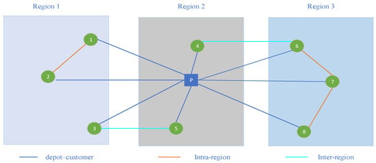
Owing to construction-related closures, hazmat-restricted segments, and dead-end roads, direct connections do not exist between certain customer pairs; consequently, urban road networks are generally not complete graphs. This paper considers an incomplete underlying road network G_road = (N, A^∗) consisting of a depot and multiple customers. Let N denote the set of all nodes, and let A^∗ denote the set of permissible direct travel links on G_road, constructed by geographic and administrative criteria to reflect realistic road connectivity. An edge (i, j) ∈ A^∗ exists if and only if at least one of the following holds (see Figure 1): (i) one of the two nodes is the depot, so that the depot is directly connected to every customer; (ii) both customers lie within the same administrative region and the distance between them falls below a predefined threshold; or (iii) the two customers belong to adjacent administrative regions and the distance between them falls below a larger threshold. Routing decisions are made on an auxiliary graph G_aux = (N, A), where each arc (i, j) ∈ A represents the shortest path from i to j on G_road (computed by Dijkstra’s algorithm [27,28]) and its cost equals the shortest-path distance; G_aux is arc-complete, while the incompleteness resides in A^∗. When the shortest path underlying an arc (i, j) passes through other nodes (the depot, or another customer not on the current vehicle’s route), the vehicle traverses them without stopping.

Figure 1. Incomplete underlying road network. Note: The letter P denotes the depot, and numbers indicate customer node identifiers; the three edge types (depot–customer, intra–region, inter–region) correspond to Rules (i)–(iii) in Section 2.1.

Under customer demand uncertainty, the depot dispatches a fleet of hazmat vehicles to serve all customers, with each vehicle completing its assigned deliveries before returning to the depot. The objective is to optimize the vehicle routes and customer service sequences so as to minimize total transport risk and total transport cost simultaneously. The following assumptions are made in this study: (i) the fleet size is finite but sufficient to cover all customer demands; (ii) the load of hazardous materials carried by each vehicle does not exceed its maximum capacity; (iii) vehicles of the same type share identical operational parameters; and (iv) hazardous incidents occurring on different edges are independent, with each incident confined to a single edge. Table 1 presents the sets, parameters, and decision variables used in the model.

Table 1. Notations.

Notations	Explanations	Notations	Explanations
N	the set of all nodes	D(i, j)	shortest-path distance between nodes i and j
Nc	the set of customer nodes	γf	risk coefficient of type f vehicle
A	the set of arcs in the auxiliary graph	[Ψ0,Ψ]	depot operating time window
A∗	the set of permissible direct travel links on the underlying road network	c4	per capita loss from a single injury (CNY/person)
F	the set of vehicle types	ε	service time (h/ton)
Kf	the set of all type f vehicles	ef	vehicle capacity (tons)
T	the set of time periods	β0	hazard coefficient of hazmat
${\tilde{q}}_i$	customer demand (tons)	β1	receptor sensitivity coefficient
c1	carbon tax rate (CNY/kg CO2e)	β2	environmental function coefficient
u	carbon emission factor for road transportation (kg/L)	β3	hazmat concentration exceedance coefficient
p	accident probability on link (i, j) (per km)	θ	hazmat release quantity (tons)
ρα	baseline population density of administrative region (persons/km2)	c3	fuel price per liter (CNY/L)
φ	impact radius of the release (km)	s	penalty cost per hour of delay when a vehicle returns to the depot after the operating hours (CNY/h)
c2	hazmat remediation cost per unit weight (CNY/ton)	$T_{\mathit{ki}}^f$	arrival time of a vehicle k (type f) at node i
vt	travel speed during time period t (km/h)	τ	uncertainty budget
λf	fuel consumption coefficient of a type f vehicle (L/km)	η(t)	population adjustment coefficient for time period t
$L_{\mathit{kij}}^f$	load of a vehicle k (type f) on link (i, j)	kf	the number of vehicles of each type
c5f	fixed usage cost (CNY/vehicle)
$x_{\mathit{kij}}^f$	binary variable indicating whether vehicle k (type f) traverses link (i, j)
$y_{\mathit{ki}}^f$	binary variable indicating whether node i is served by vehicle k (type f)

2.2. Risk Assessment Model

Following the classical probability-consequence paradigm in risk analysis, this study posits that transportation risk is governed by the joint effects of multiple dynamic factors. Specifically, link length, vehicle characteristics, load factor, population density along the route, environmental sensitivity, and the time period all significantly influence either the likelihood or the severity of an accident. For any edge (i, j), the total risk comprises two components: population exposure risk $R_{\mathit{ij}}^{\mathit{pop}}$ and environmental damage risk $R_{\mathit{ij}}^{\mathit{env}}$.

(1) Dynamic population exposure risk

When an accidental release occurs during transport, the dispersion of the hazardous material poses a threat to the safety of the surrounding population. Given a circular impact zone, the population exposure consequence is expressed as the product of the affected area, the population density, and the per capita loss from a single injury. To capture the dynamics of population distribution, coefficient η(t) is introduced to adjust the population density over time, reflecting how the population density in period t deviates from its base value.

Suppose a vehicle travels from node i to node j, whose shortest path in the incomplete road network is denoted P_ij with total length

$$D_{(i, j)}={\displaystyle \sum _{(a, b)\in {\mathrm{P}}_{\mathit{ij}}}{d}_{\mathit{ab}}}$$

(1)

where d_ab is the length of edge (a, b) on the path. For any edge (a, b), let α(a) and α(b) denote the administrative districts at its two ends, with base population densities ρ_α(a) and ρ_α(b), respectively. When the edge lies entirely within a single district, its base density ${\rho }_{\mathit{ab}}^{\mathit{base}}$ takes that district’s value; when it spans two districts, the arithmetic mean of the two districts’ base densities is used to avoid an abrupt density change at the district boundary. That is,

$${\rho }_{\mathit{ab}}^{\mathit{base}}=\left\{\begin{array}{c}{\rho }_{\alpha (a)}, \mathit{\alpha }\left(a\right)=\alpha \left(b\right)\\ {\displaystyle \frac{{\rho }_{\alpha (a)}+{\rho }_{\alpha (b)}}{2}}, \alpha \left(a\right)\ne \alpha \left(b\right)\end{array}\right.$$

(2)

The dynamic population density of edge (a, b) at time period t is

$${\rho }_{\mathit{ab}}(t)={\rho }_{\mathit{ab}}^{\mathit{base}}•\eta (t)$$

(3)

Consequently, computing the population exposure when a vehicle traverses edge (a, b) starting at time T_start and traveling at speed v_t cannot be based on a single constant density. The population exposure is defined as

$${\mathrm{E}}_{\mathit{ab}}={\displaystyle {\int }_0^{d_{\mathit{ab}}}{\rho }_{\mathit{ab}}^{\mathit{base}}•\eta (t_m)\mathit{dm}}$$

(4)

where m denotes a position along the edge and η(t_m) is the population adjustment coefficient of the period in which the vehicle passes position m. Because the speed and population adjustment coefficient are constant within each time period, they change only at period boundaries. An edge spanning more than one period is therefore discretized into short segments, within each of which both quantities remain constant. For each segment, the speed and population adjustment coefficient are determined by the time at which the vehicle traverses it, and the total population exposure along the edge is obtained by summing over all segments. The algorithm proceeds as follows:

Initialization: Set traveled distance d_tra = 0 and current time T_cur = T_start.

Iterative computation: Enter a loop until d_tra = d_ab. In each iteration:

• Determine the current period: Obtain the current travel speed v_cur and the population adjustment coefficient η(cur) from T_cur.
• Compute the next event point: Determine the earliest time T_next at which either the speed or the population coefficient may change. For example, if the current time is 9:30, the next speed-change time is 10:00, and the next population-coefficient-change time is 11:00, then the current constant-speed period lasts at most until 10:00.
• Segment the edge: Compute the maximum distance Δd_h traversable during the interval [T_cur, T_next] at speed v_cur, and take the smaller of Δd_h and the remaining distance d_re. If Δd_h < d_re, the end of the edge has not been reached and the next time period must begin. If Δd_h = d_re, the destination node b is reached within the current period.
• Accumulate exposure: Compute the population exposure contribution of this segment and add it to the running total.
• Update state: Update d_tra and T_cur, and repeat the procedure until the entire edge is traversed.

Through this procedure, the continuous population-exposure integral is approximated as a weighted sum of discrete segments:

$${\displaystyle {\int }_0^{d_{\mathit{ab}}}{\rho }_{\mathit{ab}}^{\mathit{base}}•\eta (t_m)\mathit{dm}}\approx {\displaystyle {\displaystyle \sum _{h=1}^{\mathrm{H}}}{\rho }_{\mathit{ab}}^{\mathit{base}}•}\eta (t_h)•\Delta d_h$$

(5)

where H is the number of micro-segments into which edge (a, b) is divided, and Δd_h and t_h are the length and the corresponding time for the h-th segment, respectively.

Finally, the population exposure risk is defined as

$$R_{\mathit{ij}}^{\mathit{pop}}={\displaystyle \sum _{(a, b)\in {\mathrm{P}}_{\mathit{ij}}}p\frac{L_{\mathit{kij}}^f}{e_f}{\gamma }_f{c}_4\pi {\phi }^2{\displaystyle \sum _{h\in H}\left[{\rho }_{\mathit{ab}}^{\mathit{base}}\eta (t_h)\Delta d_h\right]}}$$

(6)

(2) Environmental damage risk

A hazmat release also causes air pollution in the affected area. Let θ denote the released quantity. The damage is estimated using the imputed abatement cost method, which uses the actual cost of treating an equivalent quantity of the material, with currently available technology, as the benchmark and accounts for factors such as the hazard severity of the material, the distribution of sensitive receptors, the level of pollutant exceedance, and the environmental functional zone of the affected area [29]. The calculation formula is:

$$R_{\mathit{ij}}^{\mathit{env}}=p{D}_{(i, j)}{\gamma }_f{\displaystyle \frac{L_{\mathit{kij}}^f}{e_f}}\theta c_2\left({\beta }_0{\beta }_1+{\beta }_2\right){\beta }_3$$

(7)

2.3. Mathematical Model

The objective functions are as follows.

Objective 1: Minimization of total transport cost. Three core cost components are considered: vehicle fixed cost, fuel cost and carbon emission cost, and late-return cost. The vehicle fixed cost depends on the vehicle type; the fuel cost is linear in travel distance; and the carbon emission cost is estimated using the constant-speed fuel consumption (CSFC) metric of diesel trucks, which is widely adopted in transportation research for its computational simplicity and ease of application. The late-return cost is a penalty incurred when a vehicle returns after the depot’s closing time. The total transport cost is given by:

$$\min f_1={\displaystyle \sum _{f\in F}{\displaystyle \sum _{k\in K_f}{\displaystyle \sum _{j\in N}{c}_{5f}{x}_{k0j}^f}}}+{\displaystyle \sum _{f\in F}{\displaystyle \sum _{k\in K_f}{\displaystyle \sum _{\left(i, j\right)\in A}\left(c_{1}u+c_3\right){\lambda }_f{D}_{(i, j)}{x}_{\mathit{kij}}^f}}}+{\displaystyle \sum _{f\in F}{\displaystyle \sum _{k\in K_f}{\displaystyle \sum _{j\in N_c}\max \left(0, {\mathrm{T}}_{k0}^f-\mathsf{\Psi }\right)s{x}_{\mathit{kj}0}^f}}}$$

(8)

Objective 2: Minimization of total transport risk. The total risk aggregates the individual risks accumulated by all vehicles along their entire routes, which cover both population exposure and environmental damage. Both types of risk are converted into expected monetary losses and summed in the objective function. The total transport risk is:

$$\min f_2={\displaystyle \sum _{f\in F}{\gamma }_f{\displaystyle \sum _{k\in K_f}{\displaystyle \sum _{\left(i, j\right)\in A}p\left[{\displaystyle \sum _{(a, b)\in {\mathrm{P}}_{\mathit{ij}}}{c}_4\pi {\phi }^2{\displaystyle \sum _{h\in H}\left[{\rho }_{\mathit{ab}}^{\mathit{base}}\eta (t_h)\Delta d_h\right]}}+\theta c_2\left({\beta }_0{\beta }_1+{\beta }_2\right){\beta }_3{D}_{(i, j)}\right]}\frac{L_{\mathit{kij}}^f}{e_f}{x}_{\mathit{kij}}^f}}$$

(9)

Constraints are as follows:

$${\displaystyle \sum _{j\in N}{x}_{k0j}^f}={\displaystyle \sum _{j\in N}{x}_{\mathit{kj}0}^f\le 1}, \forall k\in K_f, f\in F$$

(10)

$${\displaystyle \sum _{j\in N:(i, j)\in A}{x}_{\mathit{kij}}^f}={\displaystyle \sum _{j\in N:(j, i)\in A}{x}_{\mathit{kji}}^f}, \forall i\in N_c, k\in K_f, f\in F$$

(11)

$${\displaystyle \sum _{f\in F}{\displaystyle \sum _{k\in K_f}{y}_{\mathit{ki}}^f}}=1, \forall i\in N_c$$

(12)

$$\left\{\begin{array}{c}{\displaystyle \sum _{j\in N:(i, j)\in A}{x}_{\mathit{kij}}^f=y_{\mathit{ki}}^f}\\ {\displaystyle \sum _{j\in N:(j, i)\in A}{x}_{\mathit{kji}}^f=y_{\mathit{ki}}^f}\end{array}\right., \forall f\in F, k\in K_f, i\in N_c$$

(13)

$$x_{\mathit{kij}}^f=0, \forall f\in F, k\in K_f, \left(i, j\right)\notin A$$

(14)

$${\displaystyle \sum _{k\in K_f}{\displaystyle \sum _{j\in N}{x}_{k0j}^f}}\le k_f, \forall f\in F$$

(15)

$${\displaystyle \sum _{i\in N_c}{\tilde{q}}_i{y}_{\mathit{ki}}^f}\le e_f, \forall k\in K_f, f\in F$$

(16)

$${\displaystyle \sum _{j\in N:(i, j)\in A}{L}_{\mathit{kij}}^f}-{\displaystyle \sum _{j\in N:(j, i)\in A}{L}_{\mathit{kji}}^f}=-{\tilde{q}}_i{y}_{\mathit{ki}}^f, \forall i\in N_c, k\in K_f, f\in F$$

(17)

$$T_{\mathit{kj}}^f\ge T_{\mathit{ki}}^f+\epsilon {\tilde{q}}_i+t_{\mathit{kij}}^f-M(1-x_{\mathit{kij}}^f), \forall f\in F, k\in K_f, \left(i, j\right)\in A$$

(18)

$${\displaystyle \sum _{i\in W}{\displaystyle \sum _{j\in W}{x}_{\mathit{kij}}^f}}\le \left|W\right|-1, W\subset N_c, W\ne \varnothing , \left|W\right|>1, \forall k\in K_f, f\in F$$

(19)

$$x_{\mathit{kij}}^f, y_{\mathit{ki}}^f\in \left\{0, 1\right\}$$

(20)

Constraint (10) ensures that vehicles depart from and return to the depot; Constraint (11) enforces route continuity; Constraint (12) guarantees that each customer is served by exactly one vehicle in one visit; Constraint (13) links the traversal and service decisions; Constraint (14) captures the topology of the incomplete network; Constraint (15) limits the number of vehicles of each type; Constraint (16) imposes the vehicle capacity limits; Constraint (17) updates the vehicle load along the route by subtracting the demand of each customer upon service; Constraint (18) describes the temporal relationship between consecutive nodes, activated only on traversed arcs through a sufficiently large constant M; Constraint (19) eliminates subtours, where W is any proper subset of the node set N_c; and Constraint (20) defines the binary decision variables.

2.4. Bertsimas–Sim Robust Optimization

Bertsimas–Sim robust optimization [30] is an approach to handling parameter uncertainty that seeks solutions whose performance remains acceptable over a specified uncertainty set. In hazmat routing, customer demand is the main source of uncertainty. By introducing an uncertainty set and the robust counterparts of the constraints, the approach hedges against demand deviations to a controllable degree: the uncertainty budget τ limits how many customers may deviate simultaneously, so that the planned routes remain feasible for the corresponding worst case.

Assume that the demand of customer i deviates from its nominal value within a box uncertainty set, i.e., ${\tilde{q}}_i\in \left[{\overline{q}}_i-{\widehat{q}}_i, {\overline{q}}_i+{\widehat{q}}_i\right]$, where ${\overline{q}}_i$ denotes the nominal demand and ${\widehat{q}}_i$ is the maximum deviation. The capacity constraint (16) under demand uncertainty becomes:

$${\displaystyle \sum _{i\in N_c}{\overline{q}}_i{y}_{\mathit{ki}}^f+g_k^f\left(y, \tau \right)\le e_f, \forall k\in K_f, f\in F}$$

(21)

where

$$g_k^f\left(y, \tau \right)=\underset{\left\{\left.S\cup \left\{\psi \right\}\right|S\subseteq N_c, \left|S\right|=\left|\tau \right|, \psi \in N_c\backslash S\right\}}{\max }\left[{\displaystyle \sum _{i\in S}{\widehat{q}}_i{y}_{\mathit{ki}}^f+\left(\tau -⌊\tau ⌋\right){\widehat{q}}_i{y}_{\mathit{ki}}^f}\right]$$

(22)

Let S denote the set of customers whose demands may deviate from their nominal values, and let τ be the uncertainty budget, which limits the maximum number of customers whose demands may deviate simultaneously; ⌊τ⌋ is the largest integer not exceeding τ. By introducing the auxiliary variable z_i(∀i ∈ N_c), constraint (22) can be rewritten as:

$$\begin{array}{l}{g}_k^f\left(y, \tau \right)=\max \left[{\displaystyle \sum _{i\in N_c}{\widehat{q}}_i{y}_{\mathit{ki}}^f{z}_i}\right]\\ s.t.{\displaystyle \sum _{i\in N_c}{z}_i}\le \tau \\ 0\le z_i\le 1, \forall i\in N_c\end{array}$$

(23)

Setting τ = 0 recovers the deterministic model with nominal demands, whereas setting τ = n allows all demands to deviate to their worst-case values, making the model equivalent to the Soyster model.

By duality theory, the dual problem of Equation (23) is

$$\begin{array}{l}\min {\varpi }_k^f\tau +{\displaystyle \sum _{i\in N_c}{\zeta }_{\mathit{ki}}^f}\\ s.t. {\varpi }_k^f+{\zeta }_{\mathit{ki}}^f\ge {\widehat{q}}_i{y}_{\mathit{ki}}^f, \forall i\in N_c\\ {\zeta }_{\mathit{ki}}^f\ge 0, \forall i\in N_c\\ {\varpi }_k^f\ge 0\end{array}$$

(24)

where ${\varpi }_k^f$ and ${\zeta }_{\mathit{ki}}^f$ are the dual variables associated with the budget constraint and the upper-bound constraints, respectively. The robust counterpart of Equation (21) is

$$\begin{array}{l}{\displaystyle \sum _{i\in N_c}{\overline{q}}_i}{y}_{\mathit{ki}}^f+{\varpi }_k^f\tau +{\displaystyle \sum _{i\in N_c}{\zeta }_{\mathit{ki}}^f}\le e_f, \forall f\in F, k\in K_f\\ {\varpi }_k^f+{\zeta }_{\mathit{ki}}^f\ge {\widehat{q}}_i{y}_{\mathit{ki}}^f, \forall i\in N_c\\ {\zeta }_{\mathit{ki}}^f\ge 0, \forall i\in N_c\\ {\varpi }_k^f\ge 0\end{array}$$

(25)

Within the robust optimization framework, only the vehicle-capacity constraint (16) is robustified by the Bertsimas–Sim approach, so that no vehicle is overloaded under the worst-case demand deviation admitted by the uncertainty set. The arc-load relation (17) and the time-propagation relation (18) are instead formulated under the nominal demand; they are treated as nominal descriptions of system operation, and used to compute travel times and dynamic risk. Accordingly, constraints (17) and (18) are restated as follows:

$${\displaystyle \sum _{j\in N:(i, j)\in A}{L}_{\mathit{kij}}^f}-{\displaystyle \sum _{j\in N:(j, i)\in A}{L}_{\mathit{kji}}^f}=-{\overline{q}}_i{y}_{\mathit{ki}}^f, \forall i\in N_c, k\in K_f, f\in F$$

(26)

$$T_{\mathit{kj}}^f\ge T_{\mathit{ki}}^f+\epsilon {\overline{q}}_i+t_{\mathit{kij}}^f-M(1-x_{\mathit{kij}}^f), \forall f\in F, k\in K_f, \left(i, j\right)\in A$$

(27)

In summary, the robust optimization model for hazmat routing under demand uncertainty consists of objective functions (8)–(9) and constraints (10)–(15), (19)–(20), and (25)–(27).

3. Solution Method

This study employs the Non-dominated Sorting Genetic Algorithm II (NSGA-II) to solve the multi-objective heterogeneous-fleet hazmat vehicle routing problem with the Bertsimas–Sim robust counterpart of the capacity constraint. NSGA-II combines fast non-dominated sorting, crowding distance, and elitist preservation, and thereby yields a well-converged and well-distributed approximation of the Pareto front. The algorithm is implemented in Python using the Distributed Evolutionary Algorithms in Python (DEAP) framework.

3.1. Encoding and Decoding

Given the combinatorial nature of the vehicle routing problem, directly encoding routes yields a complex solution space prone to infeasible solutions. An efficient indirect encoding strategy is therefore adopted.

Encoding: Each individual (chromosome) is represented as a permutation of all n customer IDs. For a problem with 30 customers, an individual may be an integer sequence such as [5, 18, 2, …, 13]. This encoding ensures that each customer appears exactly once.

Decoding: The genetic algorithm operates on permutations, whereas fitness evaluation requires a decoder that converts each permutation into a feasible multi-vehicle routing plan. The decoder follows a sequential-scan, capacity-first strategy, which proceeds as follows: (1) traverse the permutation in order; (2) assign the next customer to the current route and accumulate the nominal demand; (3) if the accumulated demand would exceed the capacity of the vehicle assigned to the current route, close the current route and return the vehicle to the depot; (4) activate the next vehicle in a predefined vehicle list and start a new route from the current customer. Smaller vehicles, which incur a lower fixed cost and carry a smaller type-specific risk coefficient, are used before larger ones; if the predefined fleet is exhausted, an additional vehicle of the largest-capacity type is appended; (5) repeat until all customers are assigned.

Upon partitioning the permutation into routes, the decoder constructs the temporal profile of each route: a vehicle departs from the depot at the start of the operating window, and the arrival time at each subsequent customer is obtained by accumulating the travel time and the service time at the preceding customer. Temporal quantities therefore propagate only along the arcs actually traversed by each vehicle, which is consistent with the conditional activation semantics of the time-propagation constraints.

3.2. Population Initialization

The initial population is generated by random permutations of the customer indices: for a problem with n customers, each individual is obtained by sampling all customer IDs without replacement, producing a permutation of length n. This procedure is repeated until the population size is reached. Every individual therefore decodes to a customer sequence in which each customer appears exactly once, and the initial population is uniformly distributed over the space of permutations, providing adequate diversity for the subsequent evolutionary search.

3.3. Fitness Evaluation

Fitness evaluation quantifies the quality of each solution (i.e., each decoded routing plan) through two objective values: total transport cost and total transport risk. A dynamic route-computation strategy is adopted so that every movement is evaluated on the actual shortest paths of the incomplete road network.

(1) Shortest-path-length computation

Before evaluation, the model constructs an incomplete graph G_road = (N, A^∗) based on predefined connectivity rules. For any trip from node i to node j in the decoded plan, Dijkstra’s algorithm is invoked to compute the shortest path length D_{(i, j)} between the two nodes.

(2) Objective function computation

Total transport cost: The fuel and carbon emission costs are accumulated along the actual trajectory of each route, and the fixed cost of each vehicle and the late-return penalty are added.

Total transport risk: Risk is accumulated edge by edge along the same trajectory, accounting for the time-varying population density, the vehicle load ratio, the vehicle-type-specific risk coefficient, and the environmental sensitivity of the affected area.

(3) Constraint handling

During evaluation, all constraints are checked, including vehicle capacity, the requirement that each customer is visited exactly once, and the robust capacity constraint (i.e., the capacity limit under demand uncertainty). Any solution that violates a constraint is penalized by adding a large penalty term to both objective values; this reduces the likelihood of selection and steers the search toward the feasible region.

3.4. Evolutionary Operators

An initial population of size 200 is generated, and the fitness of each individual is evaluated. Non-dominated sorting then partitions the population into fronts, and crowding distances are computed within each front.

(1) Selection

The selection operation comprises two phases, environmental selection and mating selection, both of which rely on non-dominated sorting and crowding distance.

• Environmental selection: After each generation, the parent population P_t and its offspring Q_t are merged into a temporary population R_t = P_t ∪ Q_t. The elite-preserving strategy then selects the best N_P individuals to form the next-generation parent population P_t+1.
• Mating selection: Crowding tournament selection is employed to choose individuals from the parent population for crossover and mutation. The procedure is as follows: two individuals are randomly drawn from the parent population, and their non-domination ranks are compared. If the ranks differ, the individual with the lower (i.e., better) rank is selected; if the ranks are equal, the individual with the larger crowding distance is selected. This strategy prioritizes individuals in sparser regions of the front, thereby maintaining population diversity.

(2) Crossover

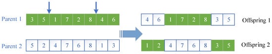
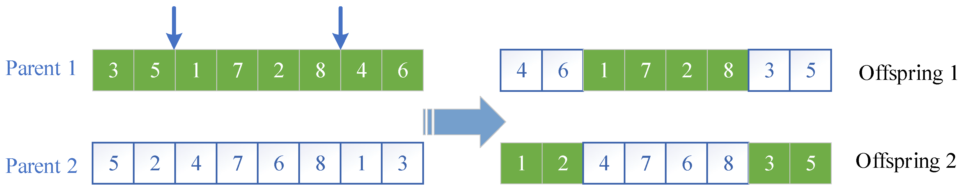
We employ the order crossover (OX) operator, which is designed for permutation-encoded problems. It randomly selects a contiguous subsequence from one parent and copies it to the corresponding positions in the offspring; the remaining positions are then filled with the genes of the second parent that are absent from the copied subsequence, taken in cyclic order starting from the position immediately after the second cut point. Crossover is applied at a fixed crossover probability. For example, with eight customers numbered 1~8, given parent 1 = [3, 5, 1, 7, 2, 8, 4, 6] and parent 2 = [5, 2, 4, 7, 6, 8, 1, 3], offspring 1 inherits positions 3~6 from parent 1, i.e., [1, 7, 2, 8]. Scanning parent 2 cyclically from position 7, the genes absent from [1, 7, 2, 8] are 3, 5, 4, 6, which fill positions 7, 8, 1, 2, respectively, yielding offspring 1 = [4, 6, 1, 7, 2, 8, 3, 5]. Symmetrically, offspring 2 inherits positions 3~6 from parent 2, i.e., [4, 7, 6, 8], and scanning parent 1 cyclically from position 7 gives the genes 3, 5, 1, 2, yielding offspring 2 = [1, 2, 4, 7, 6, 8, 3, 5]. The crossover operation is illustrated in Figure 2.

Figure 2. Schematic diagram of crossover operation. Note: Green cells indicate genes from Parent 1, and white cells indicate genes from Parent 2. Small arrows mark the two crossover points, and the large arrow indicates the generation of offspring from the parents.

(3) Mutation

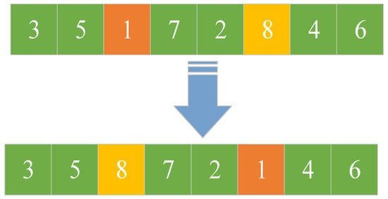
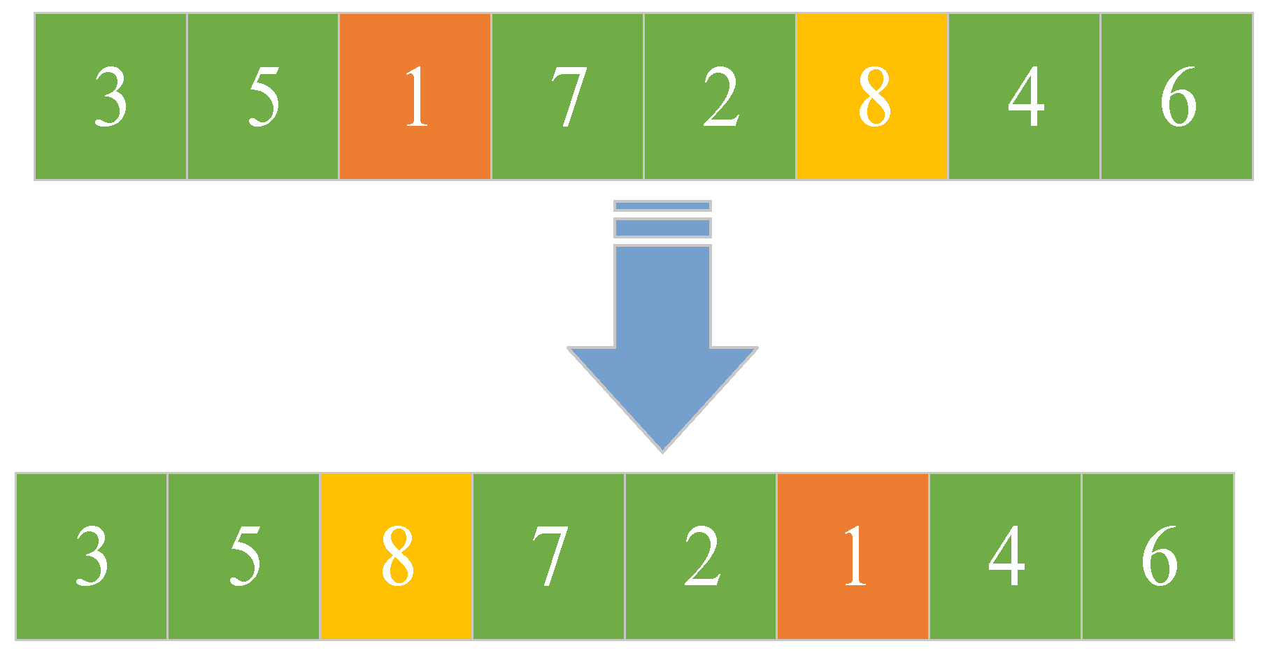
For mutation, we employ the shuffle-indexes mutation operator, designed for permutation-encoded problems. Each offspring is mutated with a fixed probability; within a mutated individual, each position is then interchanged with another randomly chosen position with an independent probability of 0.05. Because only the order of existing genes is altered, the resulting individual always remains a valid permutation. For example, given the individual [3, 5, 1, 7, 2, 8, 4, 6], if the gene at position 3 (value 1) is selected, it is interchanged with the gene at position 6 (value 8), yielding [3, 5, 8, 7, 2, 1, 4, 6]. The mutation operation is illustrated in Figure 3.

Figure 3. Schematic diagram of mutation operation. Note: Orange and yellow cells mark the two positions swapped during mutation; green cells indicate unchanged genes. The arrow indicates the transformation from the original to the mutated individual.

3.5. Algorithm Termination

The algorithm begins with a randomly generated initial population and iterates. In each generation, offspring are produced through selection, crossover, and mutation, and are then merged with the parent population to form the next-generation parent population via environmental selection. The algorithm terminates when the preset maximum of 150 generations is reached. Finally, it outputs the non-dominated solutions that approximate the Pareto front, representing the trade-off between total transport cost and total transport risk.

4. Case Study

This study uses BH, a representative chlorine plant, and part of its supply network as a case study. The node parameters are listed in Table 2: node 0 is BH’s depot, and nodes 1–30 are the customer demand points, which include water treatment plants, semiconductor firms, and biopharmaceutical companies across six administrative districts of Beijing. BH operates within the window of 9:00–17:00, and late returns incur a penalty.

Table 2. Node parameters.

Node	Coordinates	Demand	District	Node	Coordinates	Demand	District
0	(40.0031°, 116.4994°)	/	CY	16	(39.8142°, 116.3671°)	7–8	FT
1	(39.9246°, 116.3994°)	2–5	HD	17	(39.9292°, 116.1782°)	2–3	HD
2	(39.9234°, 116.3613°)	3–5	HD	18	(39.7396°, 116.1474°)	5–7	FS
3	(39.9500°, 116.3250°)	4–7	HD	19	(39.7664°, 116.2194°)	2–3	DX
4	(39.9516°, 116.3117°)	1–2	HD	20	(39.8664°, 116.3194°)	4–6	FT
5	(39.8615°, 116.3030°)	3–4	FT	21	(39.7838°, 116.5134°)	7–9	DX
6	(39.8767°, 116.5255°)	1–4	CY	22	(39.9838°, 116.5744°)	14–18	SY
7	(39.9440°, 116.4700°)	4–6	HD	23	(39.8607°, 116.4529°)	9–11	FT
8	(39.9760°, 116.3790°)	7–11	HD	24	(39.8566°, 116.3791°)	0.5–2	FT
9	(39.9500°, 116.4500°)	1–2	HD	25	(39.8738°, 116.2199°)	7–9	FT
10	(39.9271°, 116.2725°)	1–4	HD	26	(40.0237°, 116.3057°)	1–2	CY
11	(39.8402°, 116.3038°)	5–7	FT	27	(39.9655°, 116.3054°)	1–2	HD
12	(39.7986°, 116.5108°)	1–2	DX	28	(39.7921°, 116.2835°)	1–2	DX
13	(39.8300°, 116.1550°)	2–5	FS	29	(39.7770°, 116.5364°)	3–5	DX
14	(39.8258°, 116.1795°)	2–3	FS	30	(39.7621°, 116.3609°)	3–4	DX
15	(39.8501°, 116.3668°)	5–6	FT

The depot is directly connected to every customer node, so that each vehicle can depart from and return to the depot. Rules (ii) and (iii) are specified as follows: the two nodes lie in the same administrative district and are less than 15 km apart, or they lie in adjacent districts and are less than 25 km apart. Under these rules, the edge density of the road network is approximately 52%.

4.1. Parameter Settings

(1) Case parameter configuration

To reflect the time-varying characteristics of urban road-network speeds, the transportation time window 9:00–17:00 is divided into three periods based on Beijing weekday traffic patterns and hazmat transport safety requirements: morning peak 9:00–11:00, midday off-peak 11:00–14:00, and afternoon off-peak 14:00–17:00. Average link speeds for each period are calibrated using real-time road-network data published by the Beijing Municipal Transportation Commission, and speed is assumed constant within each period. The parameters are set as follows: p = 10⁻⁶, c₁ = 0.097, c₂ = 8000, c₃ = 6.9, c₄ = 500, c_5f = [200, 350], β₀ = 1.75, β₁ = 1.2, β₂ = 1.5, β₃ = 1.3, u = 2.6765, θ = 0.5, s = 6000, k_f = [8, 8], e_f = [10, 20], γ_f = [1, 1.2], v_t = [26.68, 32.08, 29.61], η(t) = [1.1, 0.9, 1.0], λ_f = [0.25, 0.4], ε = 0.16. For computational convenience, the real population data were scaled, with the base population densities of the CY, FT, DX, HD, FS, and SY districts set to 756, 656, 193, 725, 66, and 130 persons per km², respectively. The atmospheric dispersion of an accidental release of 0.5 tons of chlorine was simulated with ALOHA using meteorological data for Beijing, which yielded a threat zone radius of 2.90 km.

(2) Algorithm tuning

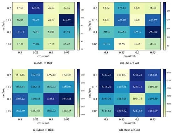
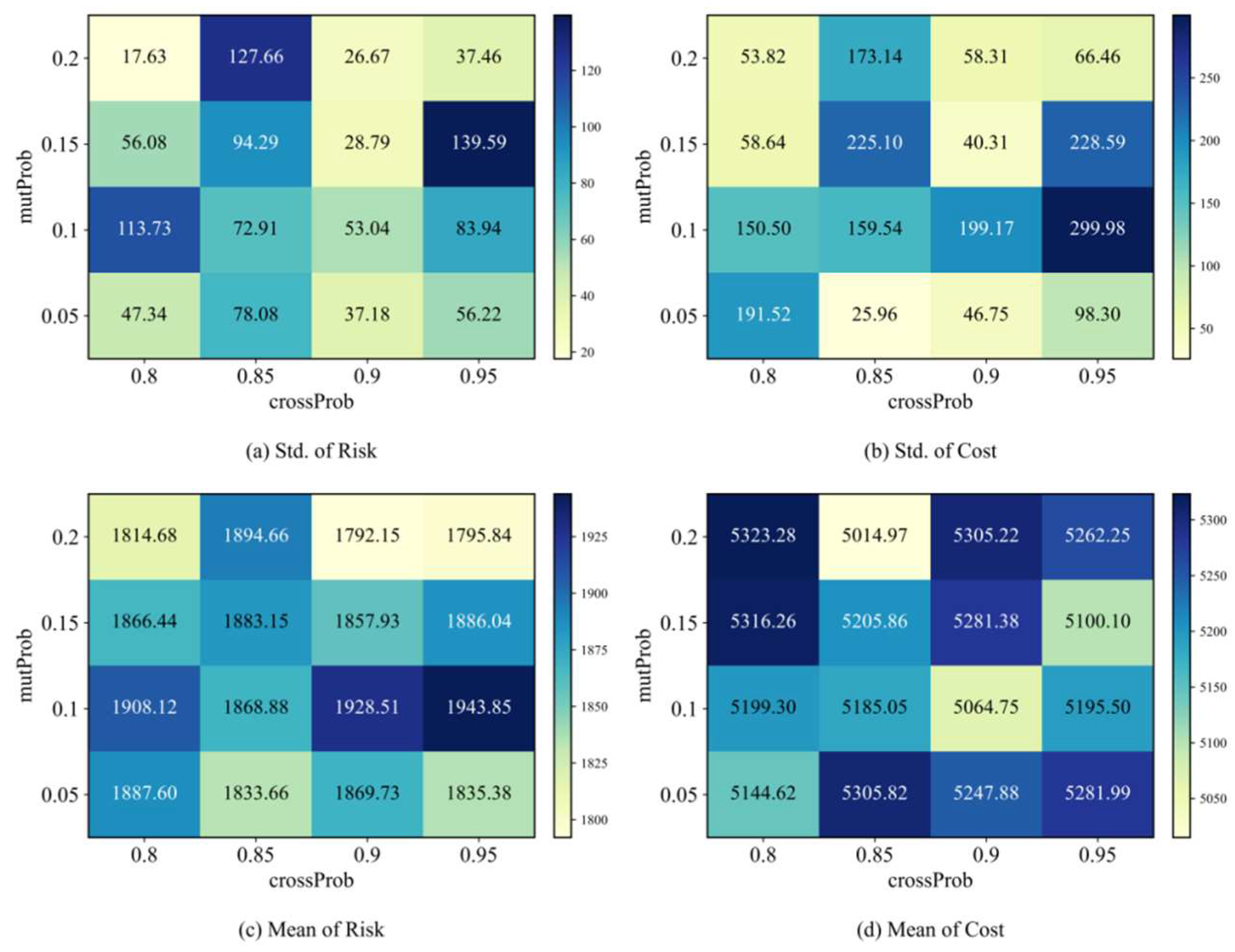
A grid search is conducted over crossProb ∈ {0.80, 0.85, 0.90, 0.95} and mutProb ∈ {0.05, 0.10, 0.15, 0.20}, with each of the 16 combinations run multiple times under the same computational budget. A two-stage screening strategy is adopted: (i) stability is first assessed via the standard-deviation index,

Φ₁ = norm(σ_cost) + norm(σ_risk)

(28)

where norm(•) is a normalization operation, and σ_cost and σ_risk are the standard deviations of cost and risk across repeated runs. The top 25% of combinations by stability are selected as candidates. (ii) Within the candidate set, the mean cost and mean risk are normalized, and an equal-weight composite score is computed:

Φ₂ = 0.5norm(μ_cost) + 0.5norm(μ_risk)

(29)

where μ_cost and μ_risk are the mean cost and mean risk across repeated runs.

Figure 4 presents the cost and risk heatmaps. Lighter cells indicate better performance, since cost, risk, and their standard deviations are all to be minimized. The results show that higher mutation probabilities generally reduce the standard deviation of both objectives, indicating that sufficient mutation is key to stable convergence under robust constraints. To balance performance and stability, crossProb = 0.90 and mutProb = 0.20 are selected as the unified settings for all subsequent experiments.

Figure 4. Heatmap of cost and risk.

4.2. Operation Results

The model is solved in Python 3.11 on a computer equipped with an Intel(R) Core(TM) i7-12700H processor at 2.30 GHz and 16 GB of RAM. Under the uncertainty budget τ = 2, the algorithm is run repeatedly, yielding an average total transport cost of 5233.61 CNY, an average total transport risk of 1866.77 CNY, and an average total travel distance of 688.44 km. To illustrate a concrete transportation plan, one representative run is selected for detailed analysis; its compromise solution, the non-dominated point closest to the ideal point of the corresponding Pareto front, achieves a total cost of 5251.99 CNY and a total risk of 1823.14 CNY, as reported in Table 3. In this plan, 14 vehicles are dispatched in total, of which 8 are of the small-capacity type and 6 are of the large-capacity type, and all vehicles return to the depot before 17:00.

Table 3. Route configuration and operational results of the solution.

Vehicle	Vehicle Type	Load (tons)	Customers Served	Distance (km)
No.1	Type 1	6.50	7, 26	47.37
No.2	Type 1	2.50	6	28.46
No.3	Type 1	5.50	3	31.98
No.4	Type 1	7.00	1, 5	46.00
No.5	Type 1	6.50	9, 20	43.36
No.6	Type 1	8.00	21	48.83
No.7	Type 1	5.50	12, 29	51.35
No.8	Type 1	6.75	15, 24	40.95
No.9	Type 2	11.00	16, 30	58.95
No.10	Type 2	16.00	22	13.48
No.11	Type 2	15.50	8, 27, 10, 17	58.80
No.12	Type 2	16.00	14, 13, 18, 19, 28	88.72
No.13	Type 2	13.50	2, 25, 4	56.65
No.14	Type 2	16.00	23, 11	53.88

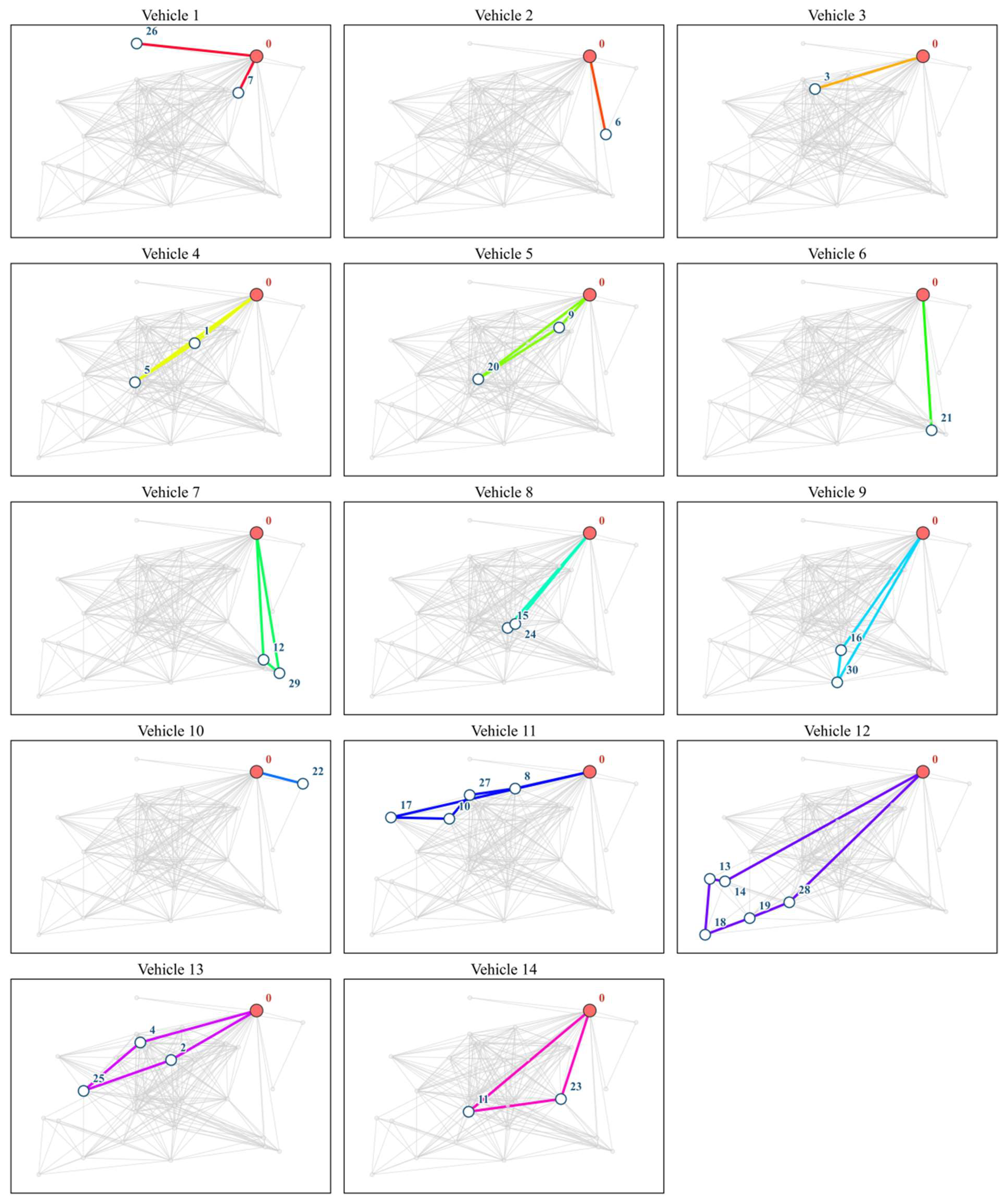
Figure 5 displays the actual travel trajectories of all vehicles on the incomplete road network G_road. The 30 customer nodes are partitioned into several geographically concentrated clusters, with a tendency to assign a single vehicle to each cluster. For example, Vehicle 12 serves the customer group in the lower left of the map, while Vehicle 7 serves the group in the lower right. Across the 14 subplots, the route shapes vary considerably and broadly fall into two categories. The first, exemplified by Vehicles 9 and 12, consists of long, complex trajectories. This strategy improves single-trip efficiency by consolidating the demands of multiple nearby customers and is key to reducing the total number of vehicles and the vehicle fixed cost. The second, exemplified by Vehicles 3 and 10, consists of simple round trips from the depot to a single customer or a few nearby customers. While this strategy increases the vehicle fixed cost, the short routes and single-customer service effectively reduce the in-transit risk and travel time, particularly for customers in isolated locations or with large demands. For Vehicle 1, the arc (7,26) is implemented as the path 7→0→26, and the vehicle passes through the depot without stopping.

Figure 5. Vehicle routing.

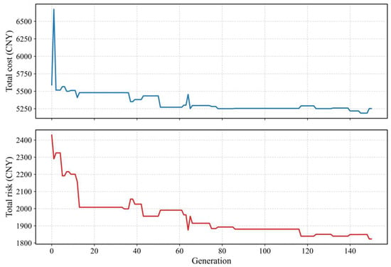
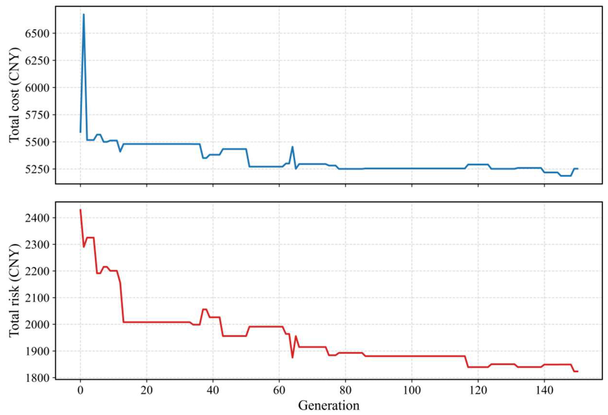
Figure 6 shows the convergence of the compromise solution over 150 generations. The early cost spike reflects the switching of the compromise point across the Pareto front (computed from normalized objectives); apart from this transient, the objective values decline rapidly in the first 15 generations and then stabilize, with cost settling around 5250 and risk around 1820 after approximately generation 100, confirming convergence.

Figure 6. Convergence curve.

4.3. Algorithm Performance Analysis

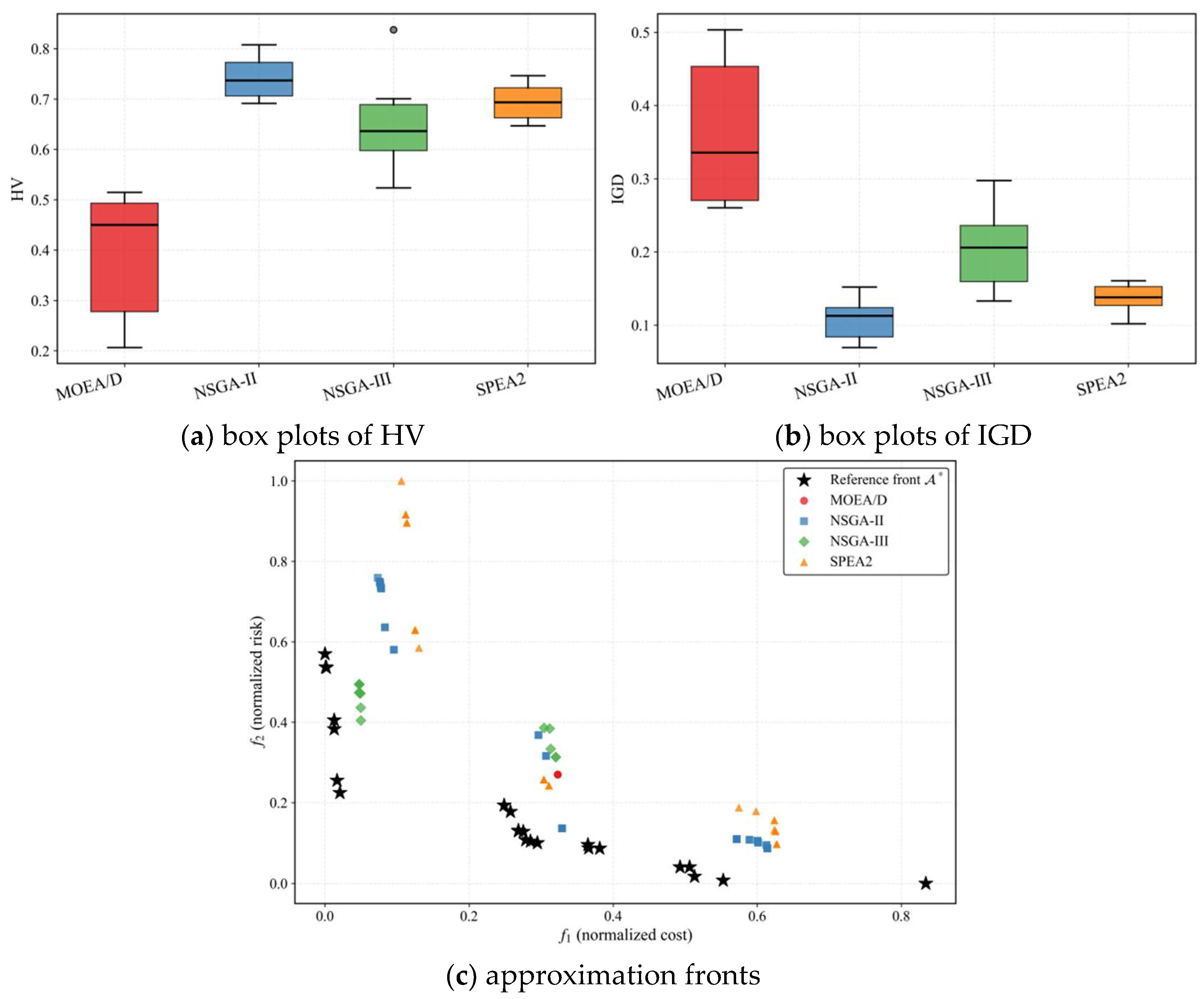
To validate the effectiveness of NSGA-II on the hazmat vehicle routing problem, it is compared with three benchmark multi-objective optimization algorithms: NSGA-III, SPEA2, and MOEA/D. The comparison is conducted at two levels. At the solution level, a compromise solution, the non-dominated solution closest to the ideal point of the Pareto front, is extracted from each run and evaluated by four scalar metrics: total cost, total risk, computational time, and total travel distance. At the front level, front quality is assessed by the hypervolume (HV) and the inverted generational distance (IGD), computed in the normalized objective space with respect to the reference front 𝒜^∗, the non-dominated subset of the union of all fronts obtained by the four algorithms; a larger HV and smaller IGD indicate better convergence and diversity. Because the number of runs per algorithm is limited and normality cannot be assumed, a Kruskal–Wallis test is first applied to each metric as an omnibus check, and each competitor is then compared with NSGA-II using the pairwise Wilcoxon rank-sum test at the 0.05 significance level. All p-values quoted in this section are those of the pairwise Wilcoxon rank-sum test.

The Kruskal–Wallis omnibus test indicates significant differences among the four algorithms on each of the six tested metrics, so the pairwise comparisons are meaningful. At the solution level, NSGA-II and SPEA2 achieve comparable cost and risk performance (cost difference 0.65%, risk difference 0.32%, p > 0.18 in both cases), while NSGA-II is significantly faster (p = 0.038). NSGA-III obtains the lowest mean cost (7.2% below NSGA-II, p = 0.003) but a higher mean risk (7.3% above NSGA-II, p = 0.007). MOEA/D is outperformed on both objectives and is markedly unstable. At the front level, NSGA-II performs best on both indicators, achieving the highest HV and the lowest IGD, and it significantly outperforms all three competitors on both (p ≤ 0.005 against NSGA-III and MOEA/D, p = 0.026 against SPEA2). SPEA2 ranks second, NSGA-III ranks third, and MOEA/D is the weakest on both indicators. The ordering therefore rests not on mean values alone but on the pairwise tests summarized in Table 4.

Table 4. Comparison of the four algorithms over multiple independent runs.

	NSGA-II	NSGA-III	SPEA2	MOEA/D	KW H
Total cost (CNY)	5233.61 ± 165.24	4858.82 ± 184.40 −	5267.61 ± 118.34 =	6122.18 ± 1368.29 +	24.00
Total risk (CNY)	1866.77 ± 96.34	2002.66 ± 72.26 +	1872.66 ± 42.71 =	2339.67 ± 314.83 +	23.61
Total distance (km)	688.44 ± 29.65	666.97 ± 25.41 =	696.10 ± 25.87 =	827.38 ± 90.38 +	19.63
Computational time (s)	783.92 ± 63.98	718.85 ± 88.92 =	894.48 ± 106.29 +	824.03 ± 11.93 =	18.47
HV	0.742 ± 0.043	0.648 ± 0.087 +	0.693 ± 0.035 +	0.398 ± 0.125 +	28.26
IGD	0.107 ± 0.027	0.203 ± 0.053 +	0.136 ± 0.020 +	0.359 ± 0.098 +	31.08

Note. All entries are reported as mean ± sample standard deviation. Superscripts give the outcome of the pairwise Wilcoxon rank-sum test comparing each algorithm with NSGA-II at the significance level 0.05. ⁺ NSGA-II significantly better, ⁼ no significant difference, ⁻ NSGA-II significantly worse.

The box plots in Figure 7a show that NSGA-II attains the highest median HV with a narrow interquartile range, while those in Figure 7b show that it also achieves the lowest median IGD; SPEA2 displays similarly compact boxes at a slightly inferior level, whereas NSGA-III exhibits visibly larger dispersion on both indicators, indicating less stable front quality across runs. MOEA/D presents the widest boxes on both indicators, confirming its instability on this problem. Figure 7c further illustrates the geometric differences among the fronts in the normalized objective space: the fronts of NSGA-II and SPEA2 spread over a wide cost–risk range and largely overlap the reference front 𝒜^∗, with most of their solutions lying on or close to it; the front of NSGA-III occupies only a narrow central portion of the reference front and covers a visibly smaller range; and the front of MOEA/D collapses into only a few distinct points scattered away from 𝒜^∗.

Figure 7. Multi-objective performance of the four algorithms.

4.4. Robustness Analysis

To evaluate the impact of the uncertainty budget on the solution, multiple independent experiments are conducted for each of five scenarios with all other parameters fixed. The results reveal the nonlinear effect of robustness on system cost and risk, as shown in Figure 8.

When transitioning from τ = 0 to τ = 1 (i.e., introducing the minimum level of robustness), all performance metrics change noticeably: the average vehicle count increases from 13.1 to 13.7; the average total cost rises from 5045.98 to 5204.63 CNY (approximately 3.1%); the average total risk increases slightly from 1845.54 to 1863.74 CNY (approximately 1.0%); and the average total travel distance increases from 655.75 km to 697.63 km (approximately 6.4%). When the model is required to account for the worst-case demand of at least one customer, the highly optimized loading plans from the deterministic model become infeasible. The most direct and effective way to satisfy the stricter robust capacity constraint is to dispatch additional vehicles to share the load. This structural change substantially alters the entire solution, and the low standard deviation indicates that it is highly consistent across repeated runs. The increase in vehicle count directly raises the vehicle fixed cost; moreover, the expansion of the fleet and the reallocation of customers may further reduce the overall efficiency of route planning, thereby increasing the route-related cost. Each additional vehicle entails a complete round trip from the depot to its assigned customers, inevitably adding travel distance.

When the uncertainty budget τ increases from 1 to 2, all performance indicators change only marginally: total cost rises by only 0.56%, while risk, travel distance, and vehicle count remain essentially unchanged. This suggests that the model transitions from a deterministic to a robust regime at τ = 1, while further increases yield only marginal adjustments. Notably, when τ rises from 2 to 4, total cost falls by roughly 1.4%, risk by 0.45%, and distance by about 1.5%. These small non-monotonic changes should be interpreted with caution. A larger τ alters the structure of the feasible region and thus the search landscape, which may redirect the search toward different regions of the solution space; at the same time, their magnitudes are comparable to the run-to-run variability of the metaheuristic, so they may equally reflect stochastic search variation rather than a systematic effect of the budget. However, as τ further increases from 4 to 10, all indicators trend slightly upward again: cost rebounds by about 1.3%, risk by 1.6%, and distance by 1.7%. This rebound reflects the price of excessive conservatism.

4.5. Out-of-Sample Performance Under Demand Deviations

The reported transport risk in the preceding sections is evaluated at nominal loads, while this subsection evaluates how the planned routes perform when the actual demands deviate from their nominal values. Two plans are evaluated under identical realizations: (i) the robust plan (τ = 2, the 14-route compromise solution reported in Table 3, nominal cost 5251.99 CNY, nominal risk 1823.14 CNY) and (ii) the deterministic plan (τ = 0, 13-route, nominal cost 5015.93 CNY, nominal risk 1880.83 CNY). Comparing the two under the same demand perturbations quantifies both the price and the benefit of robustification.

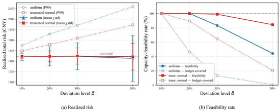
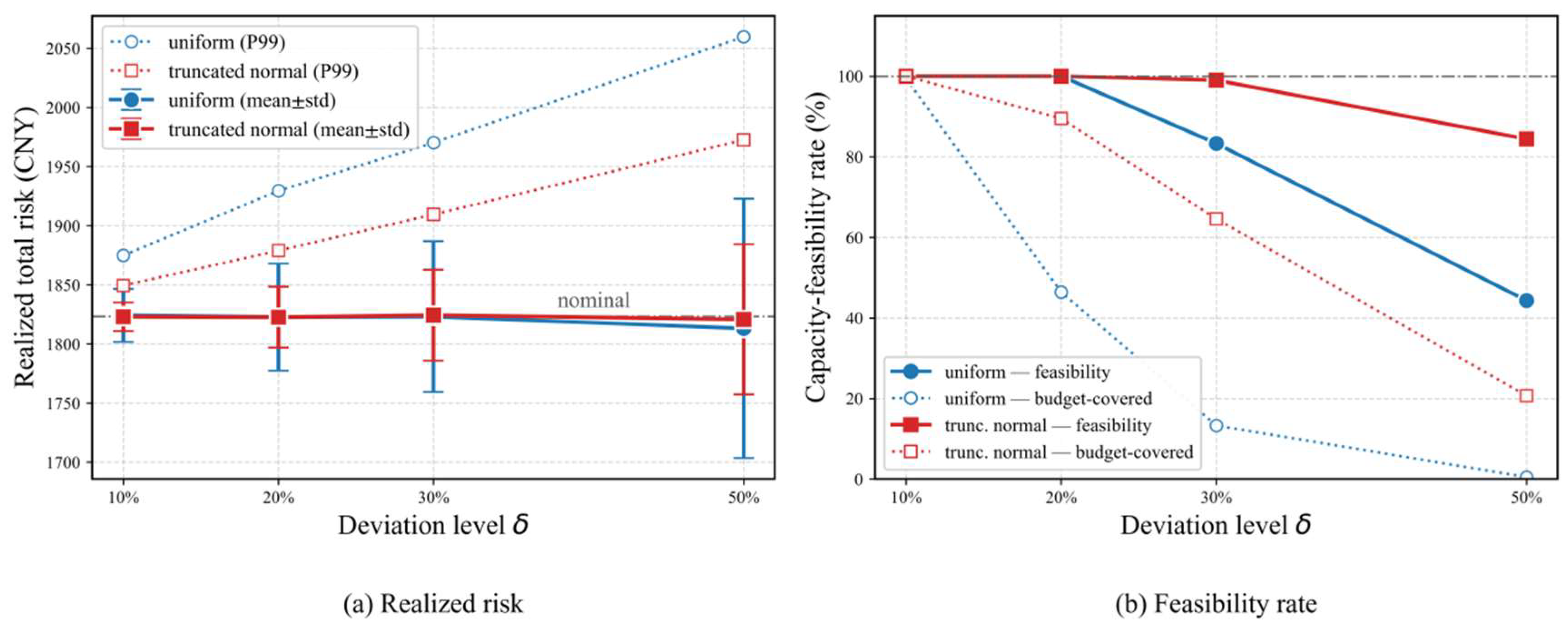
For deviation levels δ ∈ {10%, 20%, 30%, 50%}, 1000 demand realizations are drawn for each level under two sampling schemes: (1) uniform sampling, where each customer’s demand is drawn uniformly from the interval $\left[{\overline{q}}_i(1-\delta ), {\overline{q}}_i(1+\delta )\right]$; and (2) truncated-normal sampling, where the relative deviation follows a normal distribution N(0, (1/3)²) truncated to [−1, 1], so that moderate deviations near the nominal value dominate (3σ rule). For each realization and plan, we re-evaluate the routes with the same model as in planning and report the empirical capacity-feasibility rate and the realized total risk. Table 5 reports the summary statistics, and Figure 9 visualizes the realized risk and the feasibility rate as functions of δ.

Figure 8. Robustness performance variation. Note: Vehicle counts are reported as means over all runs; consequently, they may be non-integer even though each individual run yields an integer number of vehicles.

Figure 8. Robustness performance variation. Note: Vehicle counts are reported as means over all runs; consequently, they may be non-integer even though each individual run yields an integer number of vehicles.

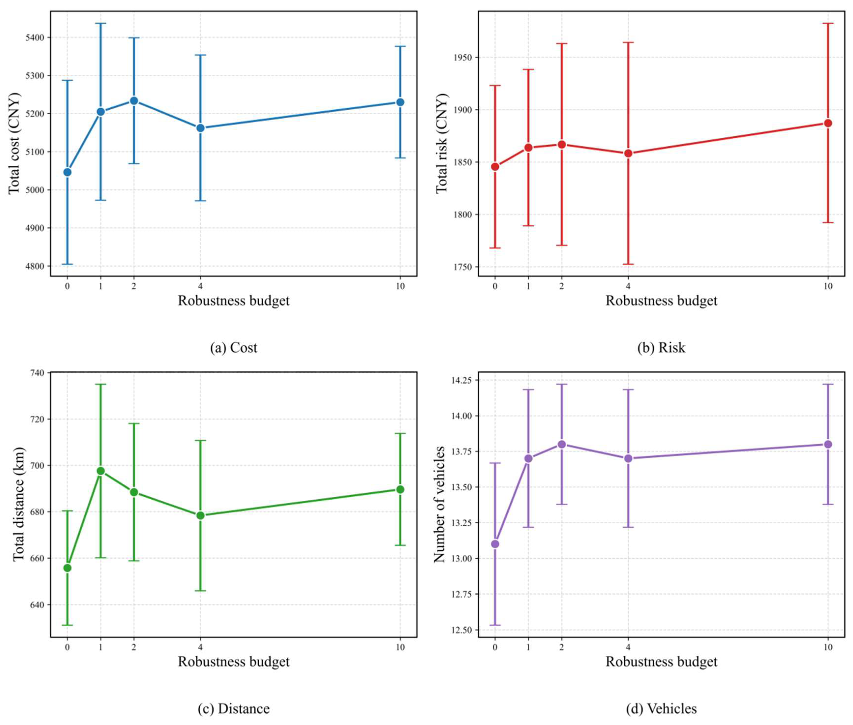
Table 5. Out-of-sample performance of the planned routes under demand deviations.

δ	Sampling	Feasibility (τ = 0)	Feasibility (τ = 2)	Budget-Covered (τ = 2)	Realized Risk (τ = 2)	Risk P99 (τ = 2)
10%	uniform	52.90%	100%	99.40%	1824.24 ± 22.38	1874.93
10%	truncated normal	51.40%	100%	100%	1823.06 ± 12.02	1849.48
20%	uniform	34.70%	100%	46.40%	1822.74 ± 45.27	1929.52
20%	truncated normal	46.60%	100%	89.50%	1822.59 ± 25.70	1878.92
30%	uniform	20.20%	83.30%	13.30%	1823.12 ± 63.84	1970.23
30%	truncated normal	40.70%	99%	64.60%	1824.35 ± 38.42	1909.52
50%	uniform	8.50%	44.30%	0.50%	1813.16 ± 109.61	2059.74
50%	truncated normal	23.50%	84.40%	20.70%	1820.77 ± 63.49	1972.64

Note: “Feasibility” is the empirical capacity-feasibility rate of the corresponding plan under each (δ, scheme) combination. The “Budget-covered” column is the share of realizations whose positive deviations are admitted by the planning budget τ = 2. To characterize the tail rather than the single largest sample, we report the 99th percentile (P99).

Figure 9. Out-of-sample performance under demand deviations (τ = 2).

Two observations follow. First, the τ = 2 plan is capacity-feasible in 100% of the realizations whose deviations fall within the worst case assumed at the planning stage, confirming the Bertsimas–Sim guarantee empirically. Beyond the budget coverage, the τ = 2 plan also remains feasible in all realizations up to δ = 20%, and retains high feasibility at δ = 30%, since its planned loads leave a capacity margin on most routes. At every deviation level, the deterministic plan (τ = 0) is far less feasible than the τ = 2 plan under the same realizations, and the gap widens monotonically with δ. At δ = 50%, the τ = 0 plan is feasible in only 8.50%~23.50% versus 44.30%~84.40% for the τ = 2 plan. The 4.71% nominal cost premium of the τ = 2 plan (5251.99 vs. 5015.93 CNY) thus buys a 36~65-percentage-point feasibility gain at δ = 10%∼50%, the benefit of robustness that complements the price of robustness documented in Section 4.4. Second, the realized total risk is centered on the nominal value and its dispersion grows with δ. The mean realized risk stays within 0.55% of the nominal value across all settings, while the standard deviation increases from 12.0~22.4 CNY at δ = 10% to 63.5~109.6 CNY at δ = 50%. The upper-tail percentiles increase moderately: the 99th percentile reaches 2059.74 CNY (uniform, δ = 50%), i.e., at most 12.98% above the nominal risk over all tested settings. The realized risk is therefore closely centered on the nominal value and bounded in the tail under the tested distributions, supporting the use of the nominal risk as a planning proxy in this instance.

5. Conclusions

This paper investigates the heterogeneous vehicle routing problem for hazardous material transportation under time-varying risk and demand uncertainty. The main contributions and findings are as follows.

(1) A time-varying risk assessment model is developed that captures the spatial heterogeneity and temporal variation in population density and incorporates vehicle-type-specific risk coefficients. Combined with an incomplete road network constructed from geographic and administrative connectivity rules, the model provides a more realistic representation of hazmat transport risk.

(2) A bi-objective robust optimization model is formulated for heterogeneous hazmat vehicle routing with per-type fleet size limits, where the Bertsimas–Sim budget controls the level of demand-uncertainty protection on vehicle capacities. The model is solved by NSGA-II and benchmarked against NSGA-III, SPEA2, and MOEA/D. NSGA-II achieves the best front quality and a favorable cost–risk balance.

(3) Sensitivity analysis reveals a nonlinear price of robustness. Introducing a minimal level of robustness restructures the fleet and routes, increasing cost, risk, and travel distance simultaneously. Once this adjustment is in place, further enlarging the uncertainty budget changes all indicators only marginally.

(4) An out-of-sample experiment spanning four deviation levels (10% to 50%) and two sampling schemes confirms that the robust plan (τ = 2) is capacity-feasible in 100% of the budget-covered realizations at every tested level and remains feasible in all sampled scenarios up to a 20% deviation. Compared with the deterministic plan (τ = 0), the 4.71% nominal cost premium delivers a 36~65-percentage-point feasibility gain across all tested deviation levels, while the mean realized risk stays within 0.55% of its nominal value (99th-percentile deviation at most 12.98%), quantifying both the price and the benefit of robustification.

Limitations and future work: Despite the contributions discussed above, two main limitations of the proposed approach should be noted. First, the Bertsimas–Sim robust protection is enforced on the vehicle-capacity constraint only; the transport risk objective is evaluated at nominal loads rather than as a worst-case risk measure. Extending the budgeted worst-case protection to the risk objective itself, which can be linearized analogously by attaching a budgeted term to the load-dependent risk contributions, is a natural direction for future work. Second, the model is a static planning tool that determines all routes a priori and does not include recourse actions once demands are realized. A promising extension is a two-stage robust formulation in which the first stage determines a priori routes while the second stage allows for localized rescheduling, such as vehicle reassignment and route adjustments, in response to demand fluctuations.

References

- Noguchi, H.; Hienuki, S.; Fuse, M. Network Theory-Based Accident Scenario Analysis for Hazardous Material Transport: A Case Study of Liquefied Petroleum Gas Transport in Japan. Reliab. Eng. Syst. Saf. 2020, 203, 107107. [Google Scholar] [CrossRef] [Scilit]
- Iranitalab, A.; Khattak, A. Probabilistic Classification of Hazardous Materials Release Events in Train Incidents and Cargo Tank Truck Crashes. Reliab. Eng. Syst. Saf. 2020, 199, 106914. [Google Scholar] [CrossRef] [Scilit]
- Hosseini, S.D.; Verma, M. Equitable Routing of Rail Hazardous Materials Shipments Using CVaR Methodology. Comput. Oper. Res. 2021, 129, 105222. [Google Scholar] [CrossRef] [Scilit]
- Li, G.; Pu, G.; Yang, J.; Jiang, X. A Multidimensional Quantitative Risk Assessment Framework for Dense Areas of Stay Points for Urban HazMat Vehicles. Reliab. Eng. Syst. Saf. 2024, 241, 109637. [Google Scholar] [CrossRef] [Scilit]
- Ke, G.Y.; Zhang, H.; Bookbinder, J.H. A Dual Toll Policy for Maintaining Risk Equity in Hazardous Materials Transportation with Fuzzy Incident Rate. Int. J. Prod. Econ. 2020, 227, 107650. [Google Scholar] [CrossRef] [Scilit]
- Liu, J.; Tan, L.; Ma, Y. An Integrated Risk Assessment Method for Urban Areas Due to Chemical Leakage Accidents. Reliab. Eng. Syst. Saf. 2024, 247, 110091. [Google Scholar] [CrossRef] [Scilit]
- Jing, Q.; Li, T.; Lai, Y.; Wang, Y.; Li, Y.; Qi, S. Study on Risk Assessment Models for the Aggregation of Vehicles Transporting Hazardous Chemicals. Reliab. Eng. Syst. Saf. 2024, 251, 110345. [Google Scholar] [CrossRef] [Scilit]
- Hu, H.; Du, J.; Li, X.; Shang, C.; Shen, Q. Risk Models for Hazardous Material Transportation Subject to Weight Variation Considerations. IEEE Trans. Fuzzy Syst. 2021, 29, 2271–2282. [Google Scholar] [CrossRef] [Scilit]
- Zhang, M.; Ding, Z.; Jiang, Q.; Wang, N. Routing Optimization for Hazardous Materials Transportation Based on Vehicle Sharing Mode. IEEE Trans. Intell. Transp. Syst. 2025, 26, 21544–21558. [Google Scholar] [CrossRef] [Scilit]
- Cui, H.; Zhao, Q.; Hua, G.; He, S.; Dong, J. A Hazardous Materials Vehicle Routing Problem with Time-Dependent Arc Capacity. Comput. Oper. Res. 2025, 183, 107187. [Google Scholar] [CrossRef] [Scilit]
- De Maio, A.; Laporte, G.; Musmanno, R.; Vocaturo, F. Sustainable Risk Mitigation in Hazardous Material Transportation. Comput. Oper. Res. 2025, 184, 107228. [Google Scholar] [CrossRef] [Scilit]
- Zandieh, F.; Ghannadpour, S.F. A Comprehensive Risk Assessment View on Interval Type-2 Fuzzy Controller for a Time-Dependent HazMat Routing Problem. Eur. J. Oper. Res. 2023, 305, 685–707. [Google Scholar] [CrossRef] [Scilit]
- Zhang, M.; Wang, N.; He, Z.; Jiang, B. Vehicle Routing Optimization for Hazmat Shipments Considering Catastrophe Avoidance and Failed Edges. Transp. Res. Part E Logist. Transp. Rev. 2021, 150, 102337. [Google Scholar] [CrossRef] [Scilit]
- Bula, G.A.; Prodhon, C.; Gonzalez, F.A.; Afsar, H.M.; Velasco, N. Variable Neighborhood Search to Solve the Vehicle Routing Problem for Hazardous Materials Transportation. J. Hazard. Mater. 2017, 324, 472–480. [Google Scholar] [CrossRef] [Scilit] [PubMed]
- Hu, H.; Li, X.; Zhang, Y.; Shang, C.; Zhang, S. Multi-Objective Location-Routing Model for Hazardous Material Logistics with Traffic Restriction Constraint in Inter-City Roads. Comput. Ind. Eng. 2019, 128, 861–876. [Google Scholar] [CrossRef] [Scilit]
- Fattahi, Z.; Behnamian, J. Location and Transportation of Intermodal Hazmat Considering Equipment Capacity and Congestion Impact: Elastic Method and Sub-Population Genetic Algorithm. Ann. Oper. Res. 2022, 316, 303–341. [Google Scholar] [CrossRef] [Scilit]
- Mohri, S.S.; Mohammadi, M.; Gendreau, M.; Pirayesh, A.; Ghasemaghaei, A.; Salehi, V. Hazardous Material Transportation Problems: A Comprehensive Overview of Models and Solution Approaches. Eur. J. Oper. Res. 2022, 302, 1–38. [Google Scholar] [CrossRef] [Scilit]
- Chai, H.; Han, W.; Dong, K.; Dai, C.; Jia, X.; Yang, L.; He, R. Multi-Modal Transport Path Optimization of Hazmat under Uncertain Demand in Hub-and-Spoke Networks. Expert Syst. Appl. 2026, 295, 128804. [Google Scholar] [CrossRef] [Scilit]
- Vaezi, A.; Dalal, J.; Verma, M. Designing Emergency Response Network for Rail Hazmat Shipments under Uncertainties: Optimization Model and Case Study. Saf. Sci. 2021, 141, 105332. [Google Scholar] [CrossRef] [Scilit]
- Wang, J.; Bai, X.; Liu, Y. Globalized Robust Bilevel Optimization Model for Hazmat Transport Network Design Considering Reliability. Reliab. Eng. Syst. Saf. 2023, 239, 109484. [Google Scholar] [CrossRef] [Scilit]
- Sun, L.; Karwan, M.H.; Kwon, C. Robust Hazmat Network Design Problems Considering Risk Uncertainty. Transp. Sci. 2016, 50, 1188–1203. [Google Scholar] [CrossRef] [Scilit]
- Jabbarzadeh, A.; Azad, N.; Verma, M. An Optimization Approach to Planning Rail Hazmat Shipments in the Presence of Random Disruptions. Omega-Int. J. Manag. Sci. 2020, 96, 102078. [Google Scholar] [CrossRef] [Scilit]
- Fang, K.; Ke, G.Y.; Verma, M. A Routing and Scheduling Approach to Rail Transportation of Hazardous Materials with Demand Due Dates. Eur. J. Oper. Res. 2017, 261, 154–168. [Google Scholar] [CrossRef] [Scilit]
- Szeto, W.Y.; Farahani, R.Z.; Sumalee, A. Link-Based Multi-Class Hazmat Routing-Scheduling Problem: A Multiple Demon Approach. Eur. J. Oper. Res. 2017, 261, 337–354. [Google Scholar] [CrossRef] [Scilit]
- Ke, G.Y. Managing Reliable Emergency Logistics for Hazardous Materials: A Two-Stage Robust Optimization Approach. Comput. Oper. Res. 2022, 138, 105557. [Google Scholar] [CrossRef] [Scilit]
- Zhao, J.; Zhang, L.; Wu, J.; Ke, G.Y. Managing Emergency Logistics for Hazardous Materials with Random Severity Level and Link Disruption: A Distributionally Robust Optimization Approach. Comput. Ind. Eng. 2025, 208, 111343. [Google Scholar] [CrossRef] [Scilit]
- Toth, P.; Vigo, D. (Eds.) Vehicle Routing: Problems, Methods, and Applications, Second Edition; Society for Industrial and Applied Mathematics: Philadelphia, PA, USA, 2014; ISBN 978-1-61197-358-7. [Google Scholar]
- Laporte, G. Fifty Years of Vehicle Routing. Transp. Sci. 2009, 43, 408–416. [Google Scholar] [CrossRef] [Scilit]
- GB/T 39793.1-2020; Ministry of Ecology and Environment, State Administration for Market Regulation. Technical Guidelines for Identification and Assessment of Environmental Damage-Principal Methods-Part 1: Imputed Abatement Cost for Air Pollution. China Environment Publishing Group Co., Ltd.: Beijing, China, 2020.
- Bertsimas, D.; Sim, M. The Price of Robustness. Oper. Res. 2004, 52, 35–53. [Google Scholar] [CrossRef] [Scilit]
Disclaimer/Publisher’s Note: The statements, opinions and data contained in all publications are solely those of the individual author(s) and contributor(s) and not of MDPI and/or the editor(s). MDPI and/or the editor(s) disclaim responsibility for any injury to people or property resulting from any ideas, methods, instructions or products referred to in the content. |
© 2026 by the authors. Licensee MDPI, Basel, Switzerland. This article is an open access article distributed under the terms and conditions of the Creative Commons Attribution (CC BY) license.