JEPADepth: Self-Supervised Monocular Depth Estimation via Joint-Embedding Predictive Architectures

Abstract

We propose JEPADepth, a self-supervised monocular depth estimation framework that augments photometric view synthesis with an auxiliary masked-prediction loss computed in the representation space of a pretrained DINOv3 Vision Transformer (ViT), following the Image Joint-Embedding Predictive Architecture (I-JEPA) principle. A predictor infers target-region embeddings from visible context-region embeddings under structured masking; the predictor and target encoder are discarded at inference, so the deployed 24 M-parameter model costs no more than the photometric-only baseline. On the KITTI Eigen split, adding the JEPA objective to an identical DINOv3 photometric baseline lowers absolute relative error from $0.105$ to $0.101$ and raises ${\delta }_1$ from $0.891$ to $0.898$, a gain roughly four times the run-to-run standard deviation measured over five random seeds. On the improved ground truth, it reaches $0.075$ absolute relative error, matching the best transformer competitor while using $11\%$ fewer inference parameters. Under zero-shot transfer without fine-tuning, it obtains the best absolute relative error on Make3D ($0.275$) and ties the best on Cityscapes ($0.143$) while leading on five of seven metrics. Training overhead is ∼16%; inference cost is unchanged.

1. Introduction

Monocular depth estimation is a core capability for 3D scene understanding, enabling applications in robotics, autonomous driving, and augmented reality [1]. While supervised learning approaches achieve strong accuracy, they require dense ground-truth depth that is expensive to obtain and often limited to specific sensors and environments. This has motivated a large body of work on self-supervised monocular depth estimation, where depth is learned directly from unlabeled videos by enforcing geometric consistency across adjacent frames.

The dominant self-supervised paradigm relies on view synthesis: a depth network and a pose network are trained such that a target frame can be reconstructed by warping source frames using the predicted depth and camera motion [2]. The photometric reconstruction error provides the main learning signal, typically complemented by smoothness and masking heuristics to mitigate occlusions and moving objects [3]. Despite its success, photometric supervision is inherently sensitive. It depends on assumptions such as brightness constancy and sufficient texture, and it can be disrupted by reflective surfaces [4,5], illumination changes [6], and non-rigid motion [7]. Moreover, because the loss is computed in pixel space, optimization can encourage solutions that memorize appearance statistics rather than enforcing higher-level scene structure [8], which can limit robustness and cross-dataset transfer [9].

In parallel, self-supervised representation learning has recently produced powerful visual encoders that capture semantic and structural regularities without manual labels. Vision Transformers [10] pretrained with large-scale objectives, such as DINOv3 [11], learn patch-level features that align with object boundaries, layout, and part structure. While these static features are highly effective for downstream tasks, depth estimation fundamentally requires reasoning about spatial geometry and occlusion. This suggests an opportunity: instead of relying solely on pixel reconstruction, self-supervised depth estimation can be regularized through feature-space predictive objectives that force the model to understand spatial relationships.

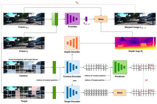
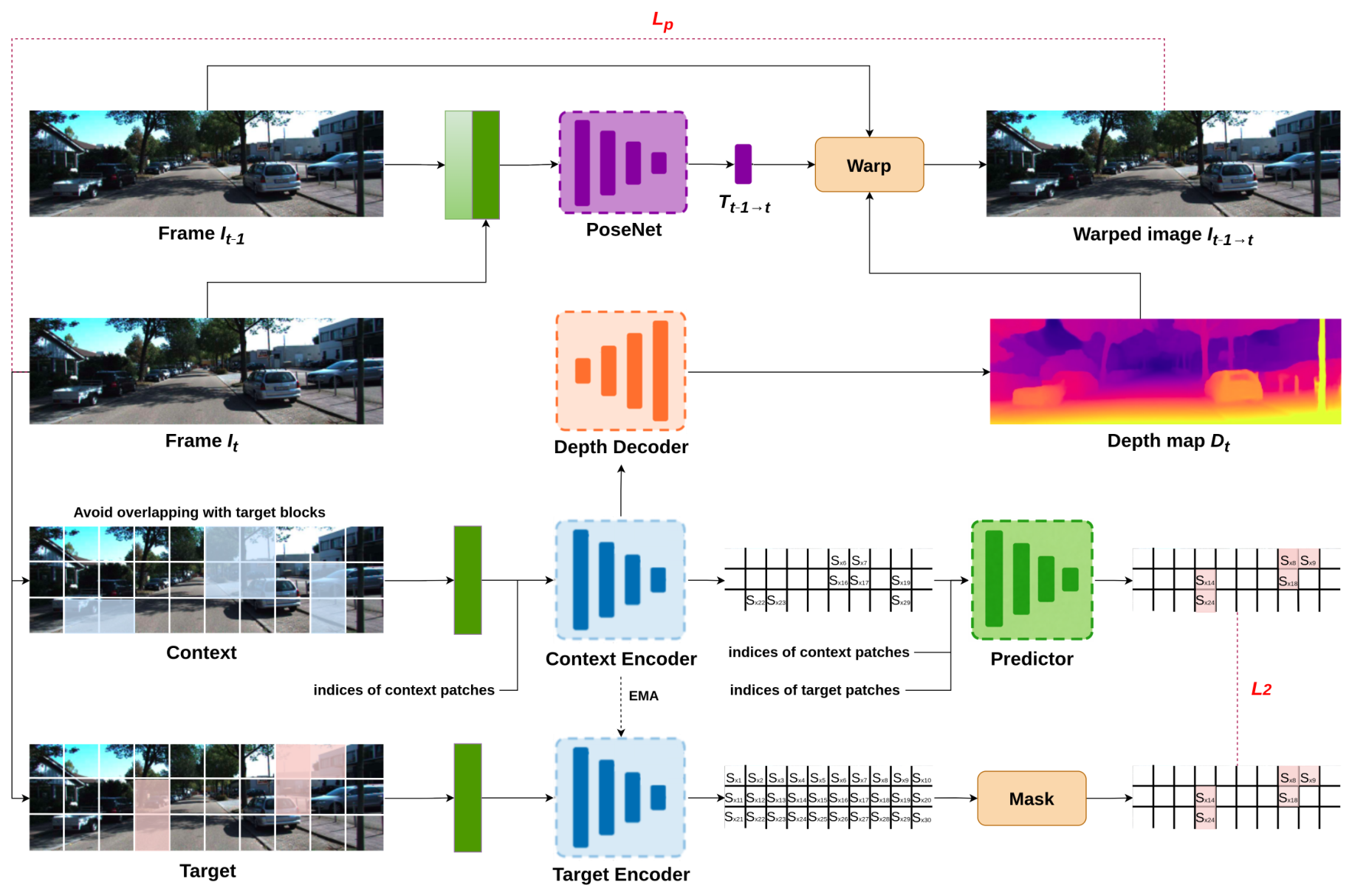
Motivated by this, we introduce JEPADepth, a self-supervised depth framework that integrates an Image Joint-Embedding Predictive Architecture (I-JEPA) [12] objective as a complementary training signal. Our approach augments a standard photometric depth pipeline with a masked predictive loss computed on patch tokens produced by a DINOv3 encoder (Figure 1). Given structured context and target masks on the patch grid, a predictor is trained to infer target-region embeddings from the visible context-region embeddings. Rather than reconstructing pixels, the JEPA-style objective encourages region-level consistency and predictive understanding in representation space. The depth network is trained end-to-end using a combination of the classical photometric loss and the JEPA representation prediction loss, yielding a model that is simultaneously constrained by multi-view geometry and regularized by predictive feature learning.

Figure 1. Overview of JEPADepth. A DINOv3 ViT encoder extracts patch tokens from the target image. A context mask selects visible tokens (blue) that are fed to a predictor, which generates embeddings for multiple masked target regions (red). In parallel, an EMA-updated target encoder produces target-region embeddings used as stop-gradient learning targets. The predicted and target embeddings are matched with a JEPA loss, which is combined with the standard photometric view-synthesis loss to train the depth network end-to-end.

A central motivation of this design is to improve robustness beyond the training distribution. Photometric self-supervision can be sensitive to appearance changes (e.g., illumination, texture, and camera characteristics), which can degrade cross-dataset transfer. We therefore add a masked prediction objective in representation space as an auxiliary training signal. The choice of space matters: the photometric loss supplies gradient only where brightness constancy holds, leaving the encoder unconstrained in textureless, specular, and dynamic regions, and an auxiliary loss reconstructing raw pixels would fill that gap with an equally appearance-bound signal. Predicting in representation space instead constrains the encoder densely everywhere and anchors fine-tuning to the pretrained feature manifold, a distinction we ablate directly in Section 4.8.5. Empirically, on KITTI, we observe improved in-domain accuracy when adding the JEPA loss to the same DINOv3-based photometric model. Moreover, a model trained on KITTI shows stronger zero-shot results on Make3D and Cityscapes without fine-tuning, indicating improved transfer under this evaluation protocol.

Our main contributions are as follows:

• JEPA-regularized self-supervised depth estimation. We propose integrating an I-JEPA-inspired masked representation prediction objective into a standard self-supervised monocular depth pipeline based on photometric view synthesis, leveraging a pretrained DINOv3 encoder to perform predictions directly in representation space rather than pixel space. Relative to Monodepth2 [3], we retain the identical photometric/pose pipeline but replace the convolutional neural network (CNN) encoder with a pretrained DINOv3 ViT and add the auxiliary representation-space objective; relative to pixel-space masked-image-modeling regularizers such as MIMDepth [13], our prediction is performed in latent space against an exponential moving average (EMA) target encoder rather than by reconstructing raw pixels, a difference we ablate directly in Section 4.8.5.
• Improved performance over a strong baseline. We show that adding the I-JEPA loss to a DINOv3-based photometric depth framework yields better results than training with photometric supervision alone. Because the predictor and target encoder are discarded after training, these gains are achieved without adding computational overhead during inference.
• Enhanced generalization under domain shift. With training on KITTI only, we report zero-shot evaluation on Cityscapes and Make3D without fine-tuning, where the proposed objective improves results under these benchmarks.

2. Related Work

2.1. Self-Supervised Depth Estimation

In the absence of ground-truth depth annotations, self-supervised monocular depth estimation methods exploit geometric consistency in visual data. SfMLearner [2] established the dominant paradigm: jointly training a depth and pose network using photometric reconstruction loss. Subsequent works introduced robust losses [14,15], feature-level consistency [16], auxiliary signals [17], and strategies for dynamic objects [3,18,19]. Transformer-based encoders further improved accuracy [20,21], and more recently, structured state space models have been explored for long-range dependency modeling [22].

Closest to our work are feature-space self-supervised methods. Zhan et al. [16] and Shu et al. [14] augment the photometric pipeline with a cross-frame feature reconstruction loss and a feature-metric warping loss, respectively. In both cases, the auxiliary signal is a consistency between features extracted from two different frames, such as a stereo pair or a photometrically warped view. In contrast, our objective operates entirely within a single image through structured masking and a stop-gradient EMA target encoder, making it independent of the multi-view photometric objective rather than a reformulation of it. To our knowledge, JEPADepth is the first method to use an I-JEPA masked predictive objective as an online auxiliary training signal inside a photometric self-supervised depth pipeline.

A related line of work introduces masked prediction as a regularizer for self-supervised depth. MIMDepth [13] adds a pixel-space reconstruction loss alongside photometric supervision. Unlike this approach, JEPADepth performs prediction in representation space following I-JEPA [12], avoiding sensitivity to pixel-level appearance.

2.2. Joint Embedding Predictive Architecture

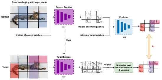
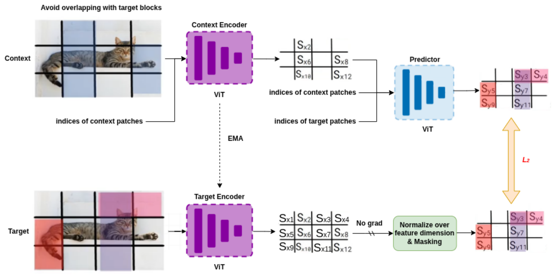
I-JEPA [12] (Figure 2) is a self-supervised framework that predicts latent representations of masked image regions from visible context patches, rather than reconstructing pixels. A context encoder processes visible patches while a momentum-updated (EMA) target encoder provides stop-gradient prediction targets. This design captures structured spatial dependencies without pixel-level supervision. The JEPA framework has since been extended to video [23], 3D point clouds [24], and world models [25]. JEPADepth does not propose a new JEPA architecture but uses the I-JEPA objective as a training signal on top of a standard photometric pipeline, a combination not explored in prior work.

Figure 2. Overview of the Image-JEPA training framework [12]. Visible context patches are processed by a context encoder, while masked target patches are encoded by a momentum-updated target encoder (EMA). A predictor maps context representations to the latent representations of target patches. The model is trained by minimizing a regression loss in feature space between predicted and target embeddings after normalization and masking. Blue shading marks the visible context patches, whereas the red, pink, and purple shaded regions denote the different target blocks.

3. Method

3.1. Self-Supervised Depth Estimation Framework

Our framework is built upon Monodepth2 [3] and follows the standard Structure from Motion (SfM) self-supervised paradigm, where a monocular camera moves through a rigid environment to provide multiple views of the same scene. We include the full derivation here for completeness.

3.1.1. Notation and View Synthesis

Let $I_t\in {\mathbb{R}}^{H\times W\times 3},t\in \{-1,0,1\}$ be a frame in a monocular video sequence captured by a moving camera, where t is the frame time index. Let $D_t\in {\mathbb{R}}^{H\times W}$ denote the depth map corresponding to image $I_t$. The camera pose change from time 0 to time $t\in \{-1,1\}$ is encoded by a $3\times 3$ rotation matrix $R_t$ and a translation vector ${\mathbf{t}}_t$. We obtain the $4\times 4$ camera transformation matrix:

$$M_t=\left[\begin{array}{cc}{R}_t& {\mathbf{t}}_t\\ 0& 1\end{array}\right].$$

(1)

Equation (1) is the standard rigid-body ($SE\left(3\right)$) transformation between the two camera coordinate frames of a moving monocular camera in a static scene. We assume: (i) the scene is rigid and static between frames, so a single global $SE\left(3\right)$ transform relates the viewpoints; (ii) $R_t\in SO\left(3\right)$ is a proper rotation ($R_t^{\top }{R}_t=I$, $\det R_t=1$) and ${\mathbf{t}}_t\in {\mathbb{R}}^3$ the camera-center translation from the reference frame $t=0$ to frame t; and (iii) the pose network predicts the 6-DoF relative pose from which $M_t$ is assembled. Violations of assumption (i) by dynamic objects are handled separately by the auto-masking of Equation (16).

Our aim is to train two networks to simultaneously estimate the pose of the camera and the structure of the scene:

$$M={\theta }_{\mathrm{pose}}\left(I_t\right),D={\theta }_{\mathrm{depth}}\left(I_t\right).$$

(2)

Self-supervised depth prediction reformulates the learning task as a novel view-synthesis problem. During training, the coupled network synthesizes the photometric appearance of a target frame from a source frame viewpoint, using the depth map as an intermediate variable.

3.1.2. Perspective Projection and Backprojection

Let $(u,v)\in {\mathbb{R}}^2$ be the calibrated pixel coordinates in image $I_0$, with origin $(0,0)$ at the top-left. A 3D point $(X,Y,Z)\in {\mathbb{R}}^3$ projects onto $(u,v)$ through the perspective projection operator:

$$\pi (X,Y,Z)=\left(f_x{\displaystyle \frac{X}{Z}}+c_x,f_y{\displaystyle \frac{Y}{Z}}+c_y\right)=(u,v),$$

(3)

where $(f_x,f_y,c_x,c_y)$ are the camera intrinsic parameters. Equations (3)–(5) are the standard pinhole projection, backprojection, and inverse-warping composition [26]. Given a depth map $D(u,v)$, a 2D point $(u,v)$ backprojects to 3D via

$${\pi }^{-1}(u,v,D(u,v))=D(u,v){\left({\displaystyle \frac{u-c_x}{f_x}},{\displaystyle \frac{v-c_y}{f_y}},1\right)}^{\top }=(X,Y,Z).$$

(4)

3.1.3. Differentiable Warping

The corresponding pixel location in source frame $I_t$ is computed by composing backprojection, pose transformation, and projection:

$$(\tilde{u},\tilde{v})=\pi \left(M_t{\pi }^{-1}(u,v,D(u,v))\right)=g(u,v\mid D(u,v),M_t).$$

(5)

Here, integer pixel indices on the grid are written $(u,v)\in \Omega \subset {\mathbb{Z}}^2$, while the reprojected coordinates $(\tilde{u},\tilde{v})\in {\mathbb{R}}^2$ are continuous. Since $(\tilde{u},\tilde{v})$ are continuous-valued, we apply differentiable bilinear sampling as in Spatial Transformer Networks [27]:

$$I^s(u,v)=\sum _i\sum _j{w}^{ij}{I}_t(u^i,v^j),$$

(6)

where $(u^i,v^j)$, $i,j\in \{1,2\}$, are the four integer-grid neighbors of $(\tilde{u},\tilde{v})$, $w^{ij}$ is proportional to the spatial proximity between $(\tilde{u},\tilde{v})$ and $(u^i,v^j)$, and ${\sum }_{i,j}{w}^{ij}=1$.

3.2. JEPADepth: JEPA-Regularized Self-Supervised Depth Training

We now describe JEPADepth, our approach for integrating an I-JEPA objective into a standard self-supervised monocular depth estimation framework. The photometric machinery of Section 3.1 and the representation-learning machinery introduced here share a single encoder but are otherwise independent objectives: the coordinate conventions of Section 3.1 play no role in the JEPA loss, which is defined entirely in feature space. The core idea is to complement pixel-space photometric supervision with a masked prediction loss in representation space, computed over patch-level tokens produced by a pretrained DINOv3 encoder. We hypothesize that this additional objective anchors the encoder to its pretrained feature manifold during photometric adaptation, limiting the extent to which fine-tuning erodes the cross-domain structure that DINOv3 pretraining encodes. The photometric loss provides gradient signal only where brightness constancy holds, leaving the encoder free to drift in textureless, specular, or dynamic regions; the JEPA loss adds a dense feature-space signal that requires the encoder to remain self-predictable under masking against a slowly-updated EMA target, acting as a self-distillation regularizer that keeps fine-tuning close to the pretrained manifold. This interpretation is supported by our ablations: the JEPA benefit is large when DINOv3 pretraining is used but minimal without it (Section 4.8.2), indicating the objective preserves and exploits pretrained features rather than supplying new geometric signal.

3.2.1. Patch-Token Representation Backbone

Given an input image $I\in {\mathbb{R}}^{H\times W\times 3}$, a Vision Transformer encoder produces a sequence of patch tokens. We use a pretrained DINOv3 ViT and extract patch-wise features

$$\mathbf{Z}=E\left(I\right)\in {\mathbb{R}}^{N\times d},$$

(7)

where $N={\displaystyle \frac{H}{P}}\times {\displaystyle \frac{W}{P}}$ is the number of patches for patch size P, and d is the embedding dimension. Unlike pixel reconstruction, these tokens capture higher-level structure such as object boundaries and layout, which we leverage as the feature space for predictive learning.

3.2.2. Depth Decoder

To predict depth, we attach a lightweight convolutional decoder $D_{\omega }$ to the encoder features. Given the patch-token embeddings $\mathbf{Z}$, the decoder upsamples and fuses multi-scale features to produce a disparity map $\widehat{d}$:

$$\widehat{d}=D_{\omega }\left(\mathbf{Z}\right).$$

(8)

We follow the standard design used in self-supervised monocular depth estimation (e.g., [3]), using lateral projections and progressive upsampling to output disparities at multiple scales, which are then used by the photometric view-synthesis loss.

The depth decoder $D_{\omega }$ is a lightweight Feature Pyramid Network (FPN)-style convolutional decoder that upsamples the patch-level ViT features to full image resolution. All ViT features enter the decoder at stride 16 (the ViT patch grid). The decoder produces multi-scale disparity outputs $\{{\widehat{d}}_0,{\widehat{d}}_1,{\widehat{d}}_2,{\widehat{d}}_3\}$, which are used by the photometric view-synthesis loss at each scale. Table 1 provides the complete architectural specification. Each scale outputs a sigmoid-activated map $\sigma \in (0,1)$ converted to depth by $d=1/(a\sigma +b)$, with $(a,b)$ set to constrain depth to a fixed range (0.1–100 m) as in [3]. The sigmoid bounds the output for numerical stability and parameterizes disparity (inverse depth), which is better conditioned across large depth ranges. Following the upsample-then-evaluate protocol of [3], each lower-resolution disparity is bilinearly upsampled to full input resolution before computing the photometric loss, and the loss is averaged over the four scales; this avoids texture-copy and hole artifacts and supplies gradient to all decoder stages. At inference only the full-resolution output ${\widehat{d}}_0$ is used.

Table 1. FPN Decoder architecture. $C_{\mathrm{in}}$ is the ViT embedding dimension (384 for ViT-S/16), $C=256$ is the decoder channel width, and $H\times W$ is the input resolution. All feature maps entering the decoder are at stride 16 (ViT patch grid).

Stage	Operation	Spatial Size	Channels	Output
Lateral ×4	$1\times 1$ Conv (no bias)	${\displaystyle \frac{H}{16}}\times {\displaystyle \frac{W}{16}}$	$C_{\mathrm{in}}\to C$	$\mathrm{lat}\left[0\right],\dots ,\mathrm{lat}\left[3\right]$
Stage 3	Upsample $\times 2$ (nearest)	${\displaystyle \frac{H}{16}}\times {\displaystyle \frac{W}{16}}\to {\displaystyle \frac{H}{8}}\times {\displaystyle \frac{W}{8}}$	C	—
	Add $\mathrm{lat}[-2]$	${\displaystyle \frac{H}{8}}\times {\displaystyle \frac{W}{8}}$	C	—
	Conv-BN-ReLU ($3\times 3$, pad 1)	${\displaystyle \frac{H}{8}}\times {\displaystyle \frac{W}{8}}$	$C\to C$	—
	Conv ($3\times 3$, pad 1) + Sigmoid	${\displaystyle \frac{H}{8}}\times {\displaystyle \frac{W}{8}}$	$C\to 1$	${\widehat{d}}_3$
Stage 2	Upsample $\times 2$ (nearest)	${\displaystyle \frac{H}{8}}\times {\displaystyle \frac{W}{8}}\to {\displaystyle \frac{H}{4}}\times {\displaystyle \frac{W}{4}}$	C	—
	Add $\mathrm{lat}[-3]$	${\displaystyle \frac{H}{4}}\times {\displaystyle \frac{W}{4}}$	C	—
	Conv-BN-ReLU ($3\times 3$, pad 1)	${\displaystyle \frac{H}{4}}\times {\displaystyle \frac{W}{4}}$	$C\to C$	—
	Conv ($3\times 3$, pad 1) + Sigmoid	${\displaystyle \frac{H}{4}}\times {\displaystyle \frac{W}{4}}$	$C\to 1$	${\widehat{d}}_2$
Stage 1	Upsample $\times 2$ (nearest)	${\displaystyle \frac{H}{4}}\times {\displaystyle \frac{W}{4}}\to {\displaystyle \frac{H}{2}}\times {\displaystyle \frac{W}{2}}$	C	—
	Add $\mathrm{lat}[-4]$	${\displaystyle \frac{H}{2}}\times {\displaystyle \frac{W}{2}}$	C	—
	Conv-BN-ReLU ($3\times 3$, pad 1)	${\displaystyle \frac{H}{2}}\times {\displaystyle \frac{W}{2}}$	$C\to C$	—
	Conv ($3\times 3$, pad 1) + Sigmoid	${\displaystyle \frac{H}{2}}\times {\displaystyle \frac{W}{2}}$	$C\to 1$	${\widehat{d}}_1$
Stage 0	Upsample $\times 2$ (nearest)	${\displaystyle \frac{H}{2}}\times {\displaystyle \frac{W}{2}}\to H\times W$	C	—
	Conv-BN-ReLU ($3\times 3$, pad 1)	$H\times W$	$C\to C$	—
	Conv ($3\times 3$, pad 1) + Sigmoid	$H\times W$	$C\to 1$	${\widehat{d}}_0$
Outputs	${\widehat{d}}_0$: full resolution	$H\times W$	1	scale 0
	${\widehat{d}}_1$: half resolution	${\displaystyle \frac{H}{2}}\times {\displaystyle \frac{W}{2}}$	1	scale 1
	${\widehat{d}}_2$: quarter resolution	${\displaystyle \frac{H}{4}}\times {\displaystyle \frac{W}{4}}$	1	scale 2
	${\widehat{d}}_3$: eighth resolution	${\displaystyle \frac{H}{8}}\times {\displaystyle \frac{W}{8}}$	1	scale 3

The design follows standard FPN principles: lateral $1\times 1$ convolutions project ViT tokens from embedding dimension $C_{\mathrm{in}}=384$ (ViT-S/16) to a uniform channel width $C=256$, followed by iterative top-down upsampling with residual addition. Each stage outputs a single-channel disparity prediction via a $3\times 3$ convolution with sigmoid activation. The total decoder has approximately 2 M parameters, making it lightweight relative to the 22 M encoder.

3.2.3. Context/Target Masking and JEPA Prediction

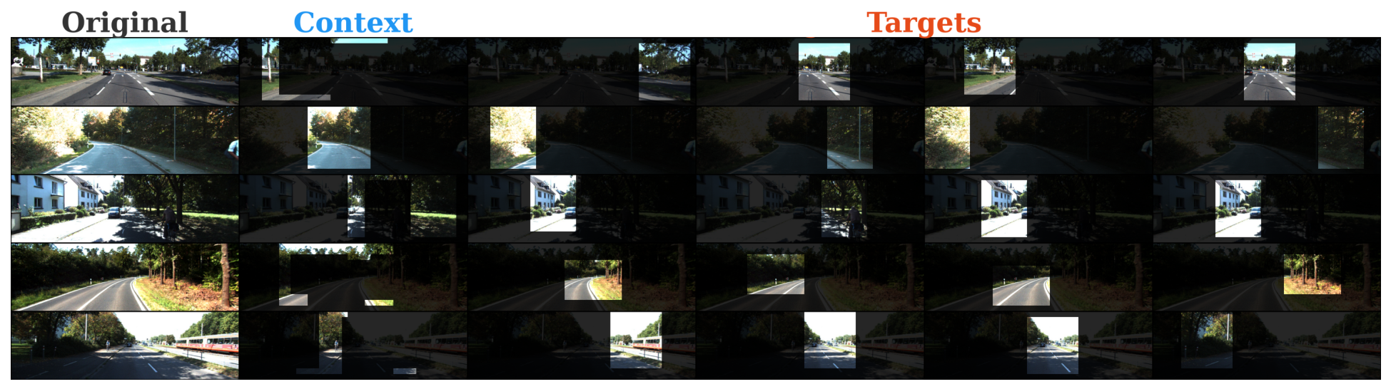
Training follows the JEPA principle: predicting representations of masked target regions from visible context regions, rather than reconstructing pixels. For each image, we sample a set of target masks ${\left\{M_{\mathrm{tgt}}^{\left(k\right)}\right\}}_{k=1}^K$ selecting held-out patch regions, together with a context mask $M_{\mathrm{ctx}}$ selecting the visible patches from which prediction is made. Masks are defined on the patch grid and can be sampled with varying scale and aspect ratio, leading to diverse spatial prediction tasks. Figure 3 shows examples of context and target blocks sampled in practice. Concretely, let the patch grid be indexed by $\Omega =\{1,\dots ,N\}$ with $N=\frac{H}{P}·\frac{W}{P}$ and patch size $P=16$. For each training image, masks are sampled by the following three-step procedure:

Figure 3. Context-target masking strategy. For each input image, we randomly sample four target regions with scales drawn from the interval $(0.15,0.2)$ and aspect ratios from $[0.75,1.5]$. Subsequently, we sample a context region with scale in $(0.85,1.0)$ and discard any overlapping target regions. This design encourages the target regions to capture semantically meaningful content, while the context region remains informative after the overlapping target patches are removed.

• Sample $K=4$ rectangular target blocks $M_{\mathrm{tgt}}^{\left(1\right)},\dots ,M_{\mathrm{tgt}}^{\left(K\right)}\subset \Omega$. Each block has an area scale drawn uniformly from $(0.15,0.2)$ of the grid and an aspect ratio drawn from $[0.75,1.5]$, positioned uniformly at random subject to fitting inside the grid. A candidate that intersects an already accepted block is rejected and resampled, so that $M_{\mathrm{tgt}}^{\left(i\right)}\cap M_{\mathrm{tgt}}^{\left(j\right)}=⌀$ for $i\ne j$.
• Sample a single candidate context block $B_{\mathrm{ctx}}\subset \Omega$ with area scale drawn uniformly from $(0.85,1.0)$, again positioned uniformly at random.
• Form the context index set by set-difference, removing from $B_{\mathrm{ctx}}$ every patch that falls inside any target block:

$$M_{\mathrm{ctx}}=B_{\mathrm{ctx}}\setminus {\displaystyle \bigcup _{k=1}^K}{M}_{\mathrm{tgt}}^{\left(k\right)}.$$

(9)

Overlap between context and target is therefore prevented by construction rather than by rejection sampling: $M_{\mathrm{ctx}}\cap M_{\mathrm{tgt}}^{\left(k\right)}=⌀$ for all k follows directly from the set-difference, so no target patch is ever visible to the predictor and the prediction task is never trivially solvable. Because the context block covers 85–$100\%$ of the grid while the four target blocks remove at most $20\%$ of it, $M_{\mathrm{ctx}}$ remains densely informative after the removal. Masks are resampled independently for every image at every training step, so the encoder sees a different spatial prediction task on each presentation.

Let ${\mathbf{Z}}_{\mathrm{ctx}}=\mathbf{Z}\left[M_{\mathrm{ctx}}\right]\in {\mathbb{R}}^{N_{\mathrm{ctx}}\times d}$ denote the context tokens. A predictor network $P_{\psi }$ takes these context embeddings and produces predictions for each target block:

$${\widehat{\mathbf{Z}}}_{\mathrm{tgt}}^{\left(k\right)}=P_{\psi }({\mathbf{Z}}_{\mathrm{ctx}},M_{\mathrm{ctx}},M_{\mathrm{tgt}}^{\left(k\right)})\in {\mathbb{R}}^{N_{\mathrm{tgt}}^{\left(k\right)}\times d}.$$

(10)

Following common I-JEPA implementations, $P_{\psi }$ is a transformer that (i) embeds the context tokens into the predictor space, (ii) concatenates learned mask tokens for the target positions with fixed sinusoidal positional embeddings, and (iii) outputs predicted target embeddings projected back to the encoder dimension. This design allows the predictor to reason over the visible region while explicitly representing the missing target locations.

3.2.4. Target Encoder and Stop-Gradient Training

To stabilize training and avoid representational collapse, we employ a target encoder $E^{\prime }$ updated as an EMA of the context encoder E. The target encoder processes the image and provides target-region embeddings:

$${\mathbf{Z}}^{\prime }=E^{\prime }\left(I\right),{\mathbf{Z}}_{\mathrm{tgt}}^{\prime \left(k\right)}={\mathbf{Z}}^{\prime }\left[M_{\mathrm{tgt}}^{\left(k\right)}\right].$$

(11)

Gradients are stopped through the target branch, and only the context encoder and predictor are updated by backpropagation through the JEPA objective:

$$L_{\mathrm{JEPA}}={\displaystyle \frac{1}{K}}{\displaystyle \sum _{k=1}^K}L2\left({\widehat{\mathbf{Z}}}_{\mathrm{tgt}}^{\left(k\right)},sg\left({\mathbf{Z}}_{\mathrm{tgt}}^{\prime \left(k\right)}\right)\right),$$

(12)

where $sg(·)$ denotes the stop-gradient operator. The target encoder parameters are updated by EMA:

$$\varphi \leftarrow m\varphi +(1-m)\theta ,$$

(13)

where $\theta$ and $\varphi$ denote the parameters of E and $E^{\prime }$, respectively, and m is a momentum coefficient.

Training is fully online and single-stage: all terms are optimized jointly with one optimizer on the summed loss of Equation (18). The shared context encoder receives gradients from both the photometric branch (via the depth decoder) and the JEPA branch (via the predictor); these are summed at the encoder. The predictor and depth decoder each receive gradients only from their own branch, the pose network only from the photometric branch, and the target encoder receives no gradient at all—the stop-gradient in Equation (12) blocks backpropagation through the target branch, which is updated solely by the EMA rule and prevents representational collapse. The two losses therefore interact only through the shared encoder parameters.

3.3. Loss Function

Objective Functions. In line with the methodologies described in [3,28], we adopt the conventional photometric loss $pe$, which is a combination of $L_1$ and Structural Similarity Index Measure (SSIM) losses:

$$pe(I_a,I_b)={\displaystyle \frac{\alpha }{2}}(1-\mathrm{SSIM}(I_a,I_b))+(1-\alpha ){∥I_a-I_b∥}_1.$$

(14)

To ensure proper depth regularization in areas lacking texture, we employ an edge-aware smooth loss, applied in the following manner:

$$L_s=\left|{\partial }_x{\widehat{d}}_t^{*}\right|e^{-\left|{\partial }_x{I}_t\right|}+\left|{\partial }_y{\widehat{d}}_t^{*}\right|e^{-\left|{\partial }_y{I}_t\right|},$$

(15)

where ${\partial }_x,{\partial }_y$ are horizontal and vertical spatial gradients (finite differences), and the $e^{-|\partial I_t|}$ term relaxes the penalty at image edges so that depth discontinuities are permitted where the image has strong gradients and penalized in smooth regions. Here, ${\widehat{d}}_t^{*}={\widehat{d}}_t/\overline{{\widehat{d}}_t}$ is the mean-normalized inverse depth, following [3]. Mean-normalization removes the global scale degree of freedom: the raw term $|\partial {\widehat{d}}_t|$ could otherwise be trivially reduced by shrinking the overall disparity magnitude toward zero (a degenerate large-depth solution), so dividing by the per-image mean makes the penalty depend only on the relative spatial structure of the disparity and prevents minimization by uniformly driving values to zero.

Photometric Auto-Masking (Image Space). This mechanism is distinct from the JEPA representation masking of Section 3.2 (Figure 3): the auto-mask $\mu$ gates the photometric loss per pixel, whereas the context/target masks $M_{\mathrm{ctx}},M_{\mathrm{tgt}}^{\left(k\right)}$ define the latent prediction task on the patch grid. In real-world settings, scenarios featuring stationary cameras and moving objects can disrupt the usual assumptions of a moving camera and static environment, negatively impacting the performance of self-supervised depth estimators. We adopt the auto-masking strategy outlined in [3], which filters out static pixels and areas of low texture that appear unchanged between two consecutive frames in a sequence. This binary mask $\mu$ is calculated as per (16), employing the Iverson bracket notation:

$$\mu =[\underset{t^{\prime }}{\min }pe(I_t,I_{t^{\prime }\to t})<\underset{t^{\prime }}{\min }pe(I_t,I_{t^{\prime }})].$$

(16)

The per-pixel photometric loss is taken as the minimum over source frames to handle occlusions [3]:

$$L_p=\underset{t^{\prime }}{\min }pe(I_t,I_{t^{\prime }\to t}).$$

(17)

Final Training Loss. We formulate the final loss by combining the masked photometric objective, the edge-aware smoothness regularizer, and the JEPA representation prediction objective. The JEPA term $L_{\mathrm{JEPA}}$ is defined in Equation (12):

$$L=\mu L_p+{\lambda }_{\mathrm{smooth}}{L}_s+{\lambda }_{\mathrm{JEPA}}{L}_{\mathrm{JEPA}},$$

(18)

where ${\lambda }_{\mathrm{smooth}}$ weights the smoothness term and ${\lambda }_{\mathrm{JEPA}}$ controls the contribution of the JEPA term. We fix ${\lambda }_{\mathrm{smooth}}={10}^{-3}$ to the standard Monodepth2 [3] value (not tuned), so that the photometric-plus-smoothness part exactly reproduces the established baseline and any change is attributable to the JEPA term. The weight ${\lambda }_{\mathrm{JEPA}}$ is tuned; the full sensitivity analysis in Section 4.8.3 shows ${\lambda }_{\mathrm{JEPA}}=1.0$ is best, with stable performance across a range of nearby values.

4. Experiments

We evaluate the effectiveness of JEPADepth on the KITTI, Cityscapes, and Make3D benchmarks. Model performance is quantified using the standard depth estimation metrics introduced in [29], enabling direct comparison with prior work.

4.1. Evaluation Metrics

We use the seven standard depth estimation metrics of [29] to quantify performance. The four error metrics are the following:

• Absolute Relative Error (AbsRel):

  $${\displaystyle \frac{1}{n}}\sum _p{\displaystyle \frac{|y_p-{\widehat{y}}_p|}{y_p}}.$$

  (19)
• Root Mean Squared Error (RMSE):

  $$\sqrt{{\displaystyle \frac{1}{n}}\sum _p{(y_p-{\widehat{y}}_p)}^2}.$$

  (20)
• Squared Relative Difference (SqRel):

  $${\displaystyle \frac{1}{n}}\sum _p{\displaystyle \frac{{(y_p-{\widehat{y}}_p)}^2}{y_p}}.$$

  (21)
• RMSE log:

  $$\sqrt{{\displaystyle \frac{1}{n}}\sum _p{(\log y_p-\log {\widehat{y}}_p)}^2}.$$

  (22)

The three threshold accuracy metrics ${\delta }_i$ measure the percentage of pixels $y_p$ satisfying

$$\max \left({\displaystyle \frac{y_p}{{\widehat{y}}_p}},{\displaystyle \frac{{\widehat{y}}_p}{y_p}}\right)=\delta <\mathrm{thr},$$

(23)

for $\mathrm{thr}=1.25,1.{25}^2,1.{25}^3$, where $y_p$ is a pixel in the ground-truth depth map y, ${\widehat{y}}_p$ is the corresponding pixel in the predicted depth map $\widehat{y}$, and n is the total number of pixels per depth map. Higher ${\delta }_i$ is better; lower is better for all error metrics.

4.2. Datasets and Experimental Protocol

4.2.1. KITTI

We evaluate JEPADepth on the widely adopted KITTI benchmark for self-supervised monocular depth estimation [30]. Following standard practice, we use the Eigen split [29], which consists of 39,810 monocular triplets for training and 4424 for validation. Our model uses a pretrained DINOv3 encoder and is fine-tuned on KITTI under a strictly monocular self-supervised setting. Specifically, training relies solely on photometric reprojection loss with auto-masking [3], without using stereo pairs, ground-truth depth supervision, or auxiliary datasets. To compare with the existing solutions, we evaluate the single-view depth performance on the test split of [31] either using raw LiDAR (697 images) or improved ground-truth labels [32] (652 images).

4.2.2. Cityscapes

To assess cross-dataset generalization, we perform zero-shot evaluation on the Cityscapes dataset [33]. Cityscapes is characterized by complex urban environments and a high density of dynamic objects, making it a challenging benchmark for generalization. We evaluate a model pretrained on KITTI directly on Cityscapes without any fine-tuning. For fair comparison with prior work, we adopt the preprocessing protocol described in [2], which converts image sequences into triplets and applies consistent cropping and resizing procedures. We report results on the 1525-image test split using the provided Semi-Global Matching (SGM) [34] disparity maps. As in the KITTI evaluation, predicted depths are clipped at 80 m, and metrics are computed only on ground-truth depth values below this threshold.

4.2.3. Make3D

To analyze robustness and generalization to a genuinely different domain, we conduct a zero-shot evaluation on Make3D [35]. Unlike Cityscapes, Make3D is not a driving dataset: it consists of outdoor campus and natural scenes (sidewalks, parks, trees, and buildings) captured with a static, tripod-mounted camera. It therefore differs from the KITTI training distribution not only in appearance but in ego-motion (no forward driving motion), scene composition (no roads, vehicles, or traffic layout), and capture setup (single static shots with no temporal sequence). This makes Make3D the more challenging of our two transfer settings, as it shares neither the motion model nor the scene geometry of the training data. The model trained exclusively on KITTI is evaluated directly on Make3D without fine-tuning, following the same image preprocessing and metrics as [3].

4.3. Implementation Details

Our method is implemented in PyTorch version 2.9.1 [36]. Unless stated otherwise, all models are trained on the KITTI dataset using the Eigen split at a resolution of $192\times 640$. We apply standard data augmentations consisting of random horizontal flips and color jitter, following common practice in self-supervised monocular depth estimation [3]. For optimization, we use Adam [37] with ${\beta }_1=0.9$ and ${\beta }_2=0.999$, a base learning rate of $1\times {10}^{-4}$, and weight decay of $1\times {10}^{-2}$. Training is run for 20 epochs with a step learning-rate schedule that decays the learning rate by a factor of $0.1$ after epoch 15 (i.e., to $1\times {10}^{-5}$ thereafter). We employ SSIM-based photometric reconstruction with $\alpha =0.85$ (as in prior work [3]) and set the disparity smoothness regularization weight to ${\lambda }_{\mathrm{smooth}}={10}^{-3}$. The training batch size is 12 and all experiments are conducted on a single NVIDIA GeForce RTX 4090 GPU.

JEPA Training Configuration

When enabling JEPA training, the depth model is built around a DINOv3 ViT-S/16 encoder [11] (∼22 M parameters) initialized from pretrained weights, coupled with a lightweight convolutional depth decoder (∼2 M parameters). The predictor is a 12-layer transformer with embedding dimension 384 (∼21 M parameters) used exclusively during training; at inference time, only the context encoder and depth decoder are retained, yielding a ∼24 M parameter inference model. The target encoder is likewise discarded at inference time. In addition to the standard photometric objective, we include a JEPA-style masked representation prediction loss with weight ${\lambda }_{\mathrm{JEPA}}=1$ selected based on a sensitivity analysis reported in Section 4.8.3, which shows that this value consistently yields the best results across all metrics. Masks are generated on the patch grid using patch size $P=16$. We adopt the masking configuration of the original I-JEPA work [12] directly, without tuning it for the driving domain, so that our comparisons isolate the effect of the JEPA objective rather than of re-tuned masking hyperparameters; these ranges were themselves selected through extensive ablation on ImageNet in [12]. The configuration uses one context mask per image covering 85–100% of patches, a large coverage shown in [12] to be critical for providing sufficient spatial signal for semantic prediction, and four target masks covering 15–20% of patches each; target masks are sampled with aspect ratio in $[0.75,1.5]$ and are constrained to be non-overlapping. The full sampling procedure and the construction that guarantees context–target disjointness are given in Section 3.2, Equation (9).

Both the context encoder and the target encoder are initialized from the pretrained DINOv3 weights. The context encoder is updated by gradient descent while the target encoder tracks it by EMA, $\varphi \leftarrow m\varphi +(1-m)\theta$, with momentum m ramped linearly from $0.996$ to $1.0$ over training. Early on ($m\approx 0.996$), the target adapts quickly, which is desirable while the context encoder is moving fastest away from initialization; a slow-updating target would produce prediction targets that are misaligned with the rapidly evolving context representation. Late in training ($m\to 1.0$), the target becomes nearly frozen, providing a low-variance, consistent prediction target that stabilizes the JEPA loss at convergence and prevents late-stage oscillation between the two encoders. This increasing momentum schedule provides crucial training stability, a principle foundational to teacher–student EMA architectures like BYOL [38] and I-JEPA [12]. We use a linear schedule for simplicity; preliminary experiments showed no significant difference with cosine scheduling on KITTI.

The additional compute introduced by the JEPA component, specifically the extra forward pass through the target encoder and the predictor, results in a modest training overhead. Training JEPADepth on KITTI for 20 epochs takes approximately 8.6 h on a single NVIDIA RTX 4090 GPU, compared to 7.4 h for the photometric-only DINOv3 baseline, representing a ∼16% increase in wall-clock training time. Critically, this overhead is incurred only during training; the predictor and target encoder are discarded at inference time, and the two models are identical in deployment cost.

4.4. KITTI Results

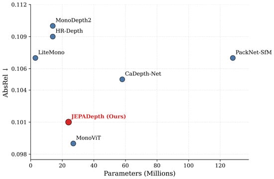
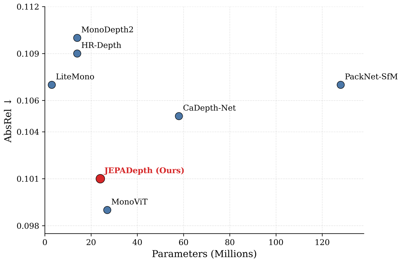
Table 2 and Table 3 report results on the KITTI Eigen split using standard and improved ground truth, respectively. JEPADepth achieves competitive performance among monocular methods, outperforming strong baselines such as Monodepth2, HR-Depth, PackNet-SfM, CADepth-Net, and Lite-Mono on both benchmarks. On the standard Eigen split, JEPADepth attains an AbsRel of $0.101$ and ${\delta }_1=0.898$, ranking second overall and surpassing all CNN-based methods while remaining competitive with MonoViT [20], which uses a larger hybrid transformer architecture. Notably, JEPADepth also achieves second-best performance on RMSE_log ($0.180$), ${\delta }_2$ ($0.965$), and ${\delta }_3$ ($0.983$) on the standard split. On the improved ground-truth benchmark, JEPADepth ties MonoViT on AbsRel ($0.075$) while using fewer parameters (24 M vs. 27 M), though MonoViT leads on the remaining metrics, and achieves second-best ${\delta }_1$ alongside DIFFNet ($0.935$). Furthermore, JEPADepth achieves this with a relatively compact model, as illustrated in Figure 4, indicating a favorable accuracy–efficiency trade-off compared to heavier methods such as PackNet-SfM (128 M) and CADepth-Net (58 M).

Table 2. KITTI (Eigen split) depth estimation results. Lower is better (↓), higher is better (↑). ${\delta }_i$ denotes $\delta <1.{25}^i$. Train: M = Monocular, MS = Monocular + Stereo, S = Stereo. All monocular methods use median scaling at test time. Bold indicates best result, underline indicates second best. JEPADepth values are single-seed for readability; across five random seeds, the standard deviation is ≤0.001 for AbsRel, RMSE_log, and ${\delta }_1$–${\delta }_3$, ≤0.007 for SqRel, and ≤0.02 for RMSE.

Method	Train	Params	H × W	AbsRel ↓	SqRel ↓	RMSE ↓	RMSElog ↓	${\mathit{\delta }}_1$ ↑	${\mathit{\delta }}_2$ ↑	${\mathit{\delta }}_3$ ↑
Monodepth2 [3]	M	14 M	$192\times 640$	0.115	0.903	4.863	0.193	0.877	0.959	0.981
Monodepth2 [3]	MS	14 M	$192\times 640$	0.106	0.818	4.750	0.196	0.874	0.957	0.979
Depth Hints [17]	S	34 M	$192\times 640$	0.102	0.762	4.602	0.189	0.880	0.960	0.981
CADepth-Net [39]	M	58 M	$192\times 640$	0.105	0.769	4.535	0.181	0.892	0.964	0.983
PackNet-SfM [40]	M	128 M	$192\times 640$	0.111	0.785	4.601	0.189	0.878	0.960	0.982
Johnston et al. [41]	M	51 M	$192\times 640$	0.106	0.861	4.699	0.185	0.889	0.962	0.982
HR-Depth [42]	M	14 M	$192\times 640$	0.109	0.792	4.632	0.185	0.884	0.962	0.983
Lite-Mono [21]	M	3 M	$192\times 640$	0.107	0.765	4.561	0.183	0.886	0.963	0.983
DIFFNet [43]	M	11 M	$192\times 640$	0.102	0.764	4.483	0.180	0.896	0.965	0.983
MonoViT [20]	M	27 M	$192\times 640$	0.099	0.708	4.372	0.175	0.900	0.967	0.984
DINOv3 w/o JEPA	M	24 M	$192\times 640$	0.105	0.861	4.710	0.186	0.891	0.961	0.981
JEPADepth (Ours)	M	24 M	$192\times 640$	0.101	0.782	4.563	0.180	0.898	0.965	0.983

Table 3. Performance comparison on KITTI improved ground truth [32]. Lower is better (↓), higher is better (↑). ${\delta }_i$ denotes $\delta <1.{25}^i$. Train: M = Monocular. All monocular methods use median scaling at test time. Bold indicates best result, underline indicates second best. JEPADepth values are single-seed for readability; across five random seeds, the standard deviation is ≤0.001 for AbsRel, RMSE_log, and ${\delta }_1$–${\delta }_3$, ≤0.008 for SqRel, and ≤0.02 for RMSE.

Method	Train	Params	H × W	AbsRel ↓	SqRel ↓	RMSE ↓	RMSElog ↓	${\mathit{\delta }}_1$ ↑	${\mathit{\delta }}_2$ ↑	${\mathit{\delta }}_3$ ↑
Monodepth2 [3]	M	14 M	$192\times 640$	0.090	0.545	3.942	0.137	0.914	0.983	0.995
HR-Depth [42]	M	14 M	$192\times 640$	0.085	0.471	3.769	0.130	0.919	0.985	0.996
PackNet-SfM [40]	M	128 M	$192\times 640$	0.078	0.420	3.485	0.121	0.931	0.986	0.996
CADepth-Net [39]	M	58 M	$192\times 640$	0.080	0.442	3.639	0.124	0.927	0.986	0.996
DIFFNet [43]	M	11 M	$192\times 640$	0.076	0.412	3.494	0.119	0.935	0.988	0.996
MonoViT [20]	M	27 M	$192\times 640$	0.075	0.389	3.419	0.115	0.938	0.989	0.997
DINOv3 w/o JEPA	M	24 M	$192\times 640$	0.077	0.476	3.724	0.123	0.932	0.985	0.995
JEPADepth (Ours)	M	24 M	$192\times 640$	0.075	0.446	3.621	0.120	0.935	0.987	0.996

Figure 4. Comparison of model efficiency and depth accuracy on KITTI using parameter count and AbsRel error. Each point corresponds to a different self-supervised monocular depth method. The plot highlights the trade-off between model size and performance, showing that JEPADepth achieves competitive accuracy with a relatively compact model, indicating a favorable accuracy–efficiency balance compared to prior approaches.

To confirm these gains are not an artifact of seed variation, we train JEPADepth over five random seeds. The run-to-run standard deviation is small (AbsRel $0.101\pm 0.001$ on Eigen and $0.075\pm 0.0004$ on improved ground truth), and the improvement over the identical photometric baseline (AbsRel $0.105\to 0.101$) exceeds this variability by roughly a factor of four, indicating the effect is well outside seed noise.

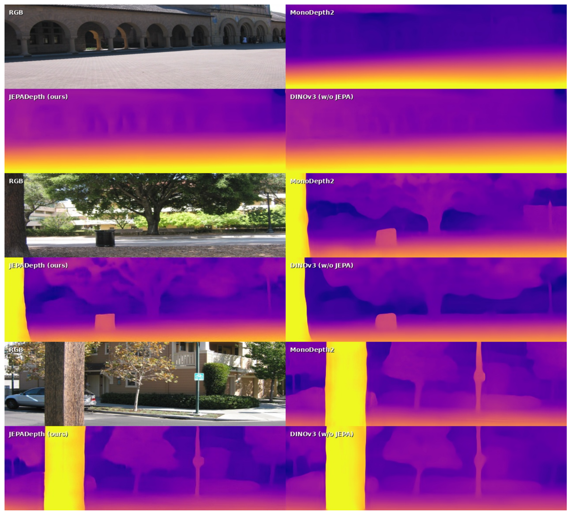
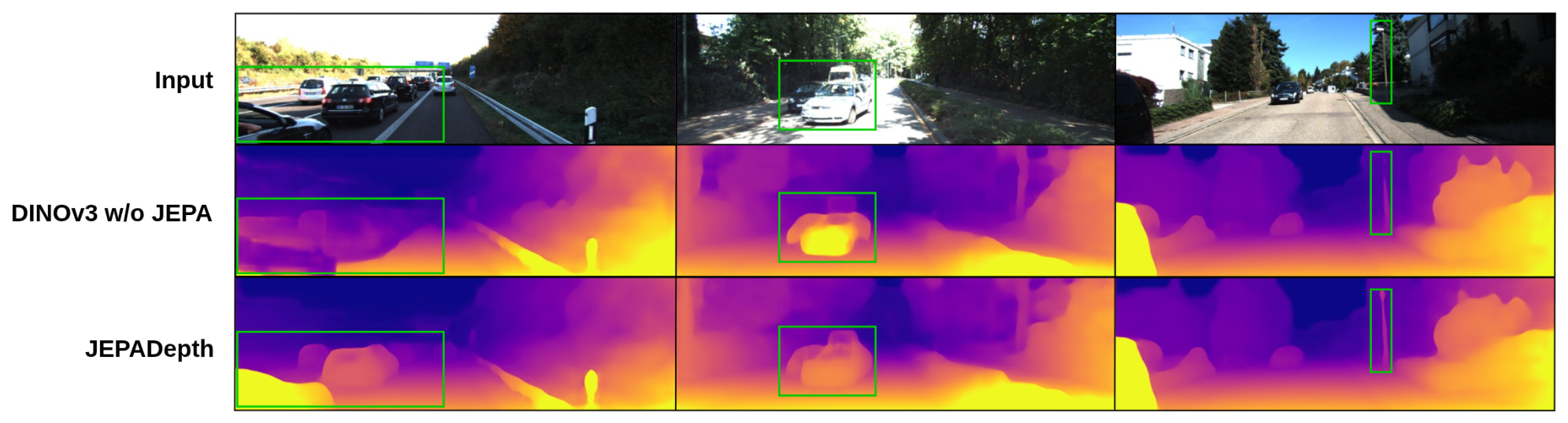
We analyze this trade-off explicitly. On the parameter–accuracy plane (Figure 4), JEPADepth lies on the Pareto front: no compared method achieves both lower AbsRel and a smaller parameter count. It matches the accuracy tier of the best transformer method, MonoViT (AbsRel $0.101$ vs. $0.099$; ${\delta }_1$ $0.898$ vs. $0.900$), with $11\%$ fewer inference parameters (24 M vs. 27 M), and clearly dominates the heavier CNN models: relative to PackNet-SfM, it reduces AbsRel by $9\%$ ($0.111\to 0.101$) while using roughly one-fifth the parameters (24 M vs. 128 M), and relative to CADepth-Net, it improves AbsRel by $4\%$ ($0.105\to 0.101$) at under half the size (24 M vs. 58 M). Crucially, the JEPA predictor (∼21 M) and target encoder are excluded from this count because they are discarded after training; the accuracy gain from the JEPA objective is thus obtained at zero additional inference-time parameter or latency cost, so the point plotted for JEPADepth reflects the same 24 M model as the DINOv3 baseline. This distinguishes our approach from the recent methods compared in Section 4.7: the only compared method with higher KITTI accuracy, HybridDepth, retains language-guidance and coarse-to-fine modules at inference, trading inference cost for accuracy in the opposite direction to ours. Qualitatively, Figure 5 and Figure 6 show this efficiency does not sacrifice structural detail, as JEPADepth recovers sharper object boundaries than the same-size DINOv3 baseline.

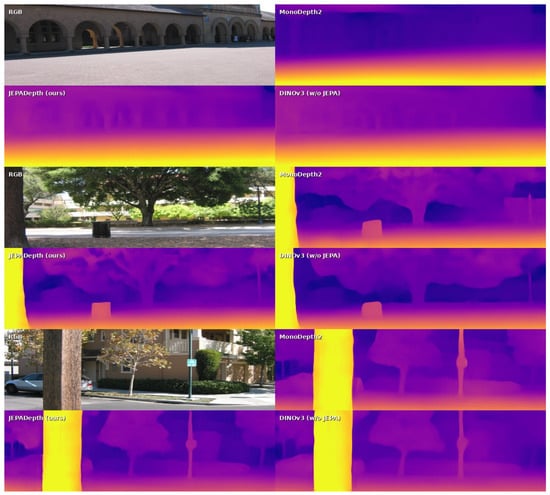
Figure 5. Qualitative depth estimation results on Make3D (zero-shot). Each row shows, from top-left to bottom-right: input RGB image, Monodepth2 prediction, JEPADepth (Ours) prediction, and DINOv3 (w/o JEPA) prediction. All models are evaluated zero-shot, trained exclusively on KITTI. JEPADepth produces structurally coherent depth maps with well-defined object boundaries, correctly separating foreground elements such as trees, poles, and buildings from the background, whereas Monodepth2 and DINOv3 (w/o JEPA) tend to produce flatter, less structured predictions that fail to recover fine-grained scene geometry under domain shift.

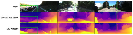
Figure 6. Qualitative KITTI results. Depth predictions on the KITTI Eigen split. JEPADepth (with the JEPA objective) recovers finer structure than the photometric-only DINOv3 baseline. Green boxes highlight the regions where the differences between the two models are most visible (vehicles in the first two columns and a thin pole in the third column). Brighter colors denote closer points (higher disparity).

Figure 6 shows qualitative depth predictions on the KITTI Eigen split. The JEPA objective yields sharper object boundaries and more coherent scene structure than the photometric-only DINOv3 baseline.

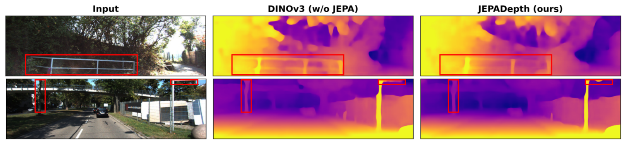
For balance, Figure 7 shows representative cases where JEPADepth does not improve over the baseline.

Figure 7. Failure cases. Two KITTI examples (red boxes) involving thin, elongated structures: a foreground metal railing (top) and a thin tree trunk with a pole (bottom). Both the photometric-only DINOv3 baseline and JEPADepth fail to recover the fine geometry of these structures, which are blurred or blended into the background; the JEPA objective provides no clear improvement here. Thin structures span very few pixels and few ViT patch tokens, so neither the photometric signal nor the patch-level representation the JEPA loss operates on carries enough spatial detail to resolve them—a limitation that motivates the higher-capacity decoder directions discussed in Section 5.

4.5. Cityscapes Results

Table 4 reports zero-shot transfer results on Cityscapes, where JEPADepth is evaluated directly without any fine-tuning using only the model pretrained on KITTI. JEPADepth ties MonoViT for the best AbsRel ($0.143$) and achieves the best performance on RMSE ($7.766$), RMSE_log ($0.208$), ${\delta }_1$ ($0.810$), ${\delta }_2$ ($0.948$), and ${\delta }_3$ ($0.985$), outperforming all competing methods on five out of seven metrics.

Table 4. Cityscapes depth estimation results. Lower is better (↓), higher is better (↑). ${\delta }_i$ denotes $\delta <1.{25}^i$. Train: K = KITTI, C = Cityscapes. All monocular methods use median scaling at test time. Bold indicates best result, underline indicates second best.

Method	Train	AbsRel ↓	SqRel ↓	RMSE ↓	RMSElog ↓	${\mathit{\delta }}_1$ ↑	${\mathit{\delta }}_2$ ↑	${\mathit{\delta }}_3$ ↑
Pilzer et al. [44]	C	0.240	4.264	8.049	0.334	0.710	0.871	0.937
Monodepth2 [3]	K	0.163	1.883	8.967	0.241	0.757	0.922	0.974
CADepth-Net [39]	K	0.150	1.691	8.527	0.227	0.786	0.931	0.978
Lite-Mono [21]	K	0.153	1.636	8.390	0.225	0.782	0.933	0.979
DIFFNet [43]	K	0.146	1.610	8.188	0.218	0.799	0.938	0.980
MonoViT [20]	K	0.143	1.485	7.981	0.211	0.803	0.942	0.983
JEPADepth (Ours)	K	0.143	1.495	7.766	0.208	0.810	0.948	0.985

4.6. Make3D Results

Table 5 reports zero-shot evaluation results on Make3D, where the model pretrained on KITTI is applied directly without any fine-tuning or domain adaptation. JEPADepth achieves the best AbsRel ($0.275$) and RMSE_log ($0.143$), outperforming all baselines including MonoViT [20] on these metrics. MonoViT obtains better SqRel ($2.758$ vs. $2.825$) and marginally better RMSE ($6.623$ vs. $6.625$). The AbsRel improvement over MonoViT ($0.286\to 0.275$) represents a relative gain of $3.8\%$, and over the strongest CNN baseline DIFFNet ($0.298\to 0.275$) a gain of $7.7\%$.

Table 5. Make3D depth estimation results. Lower is better (↓). Bold indicates best result, underline indicates second best.

Method	AbsRel ↓	SqRel ↓	RMSE ↓	RMSElog ↓
Zhou [2]	0.383	5.321	10.470	0.478
DDVO [45]	0.387	4.720	8.090	0.204
Monodepth2 [3]	0.322	3.589	7.417	0.163
CADepth-Net [39]	0.312	3.086	7.066	0.159
HR-Depth [42]	0.305	2.944	6.857	0.157
Lite-Mono [21]	0.305	3.060	6.981	0.158
DIFFNet [43]	0.298	2.901	6.753	0.153
MonoViT [20]	0.286	2.758	6.623	0.147
DINOv3 w/o JEPA	0.284	3.135	6.903	0.147
JEPADepth (Ours)	0.275	2.825	6.625	0.143

Table 5 also includes the DINOv3 baseline trained without JEPA under the same zero-shot protocol (AbsRel: $0.284$), confirming that the improvement over prior methods is not solely attributable to the DINOv3 encoder.

Qualitative results in Figure 5 further support these findings: JEPADepth produces depth maps with better scene-level understanding, correctly recovering the overall layout and relative depth ordering of outdoor structures even under significant domain shift from the KITTI training distribution. In contrast, the DINOv3 baseline without JEPA regularization tends to produce flatter, less structured predictions, suggesting that the masked predictive objective encourages the model to reason about spatial geometry rather than relying solely on local photometric cues.

4.7. Comparison with Recent Methods

To position JEPADepth within the most recent literature using published numbers (rather than as a controlled head-to-head), Table 6 lists three contemporary self-supervised methods—DaCCN [46], HybridDepth [47], and AdaDepth [48]—using their published numbers. On the standard KITTI Eigen split, JEPADepth is competitive with DaCCN (AbsRel $0.101$ vs. $0.099$) and outperforms AdaDepth (AbsRel $0.101$ vs. $0.104$). HybridDepth attains the strongest KITTI scores, though it relies on language guidance and a coarse-to-fine module that remain active at inference time, whereas the JEPA predictor and target encoder in our method are discarded after training and add no inference cost. All three methods are evaluated against the same established baselines used throughout this work (e.g., Monodepth2, DIFFNet, Lite-Mono), confirming these remain common reference points. In cross-domain transfer, HybridDepth and AdaDepth report no zero-shot results and DaCCN reports only Make3D; on Make3D, JEPADepth outperforms DaCCN on both reported metrics (AbsRel $0.275$ vs. $0.290$; SqRel $2.825$ vs. $2.873$; cf. Table 5), consistent with our finding that the JEPA objective strengthens cross-domain generalization.

Table 6. KITTI Eigen and Make3D (zero-shot) comparison with recent methods. Lower is better (↓), higher is better (↑). † = published numbers. Bold = best, underline = second. * Not reported. Numbers for DaCCN, HybridDepth, and AdaDepth are taken from the respective publications and may differ in crop, resolution, or median-scaling protocol. HybridDepth additionally uses language guidance and a coarse-to-fine inference module and is therefore not directly comparable in architecture or inference cost.

Method	KITTI Eigen				Make3D (0-Shot)
	AbsRel ↓	SqRel ↓	RMSE ↓	${\mathit{\delta }}_{\mathbf{1}}$ ↑	AbsRel ↓	SqRel ↓
DaCCN [46] †	0.099	0.661	4.316	0.897	0.290	2.873
HybridDepth [47] †	0.093	0.596	4.113	0.910	*	*
AdaDepth [48] †	0.104	0.749	4.491	0.891	*	*
JEPADepth (Ours)	0.101	0.782	4.563	0.898	0.275	2.825

4.8. Ablation Study

We conduct six ablation experiments to validate the key design choices of JEPADepth. All variants are evaluated on the KITTI Eigen split.

4.8.1. Effect of the JEPA Objective and Encoder Fine-Tuning

Table 7 shows a three-way comparison motivating JEPADepth. Freezing the DINOv3 encoder and training only the decoder yields AbsRel $0.114$, a result comparable to basic CNN baselines such as Monodepth2 ($0.115$), confirming that end-to-end adaptation is necessary to go beyond this level. End-to-end photometric fine-tuning improves this to AbsRel $0.105$. Adding the JEPA objective on top achieves the best result (AbsRel: $0.101$), improving over the no-JEPA baseline consistently across all seven metrics.

Table 7. Ablation: effect of the JEPA objective and encoder fine-tuning. Freezing the DINOv3 encoder and training only the decoder leads to performance degradation, confirming that end-to-end fine-tuning is essential. The JEPA loss further improves over fine-tuning alone. ${\delta }_i$ denotes $\delta <1.{25}^i$. Lower is better (↓), higher is better (↑). Bold indicates the best result.

Method	AbsRel ↓	SqRel ↓	RMSE ↓	RMSElog ↓	${\mathit{\delta }}_1$ ↑	${\mathit{\delta }}_2$ ↑	${\mathit{\delta }}_3$ ↑
DINOv3 frozen (decoder only) w/o JEPA	0.114	0.880	4.741	0.188	0.876	0.961	0.981
DINOv3 fine-tuned w/o JEPA	0.105	0.861	4.710	0.186	0.891	0.961	0.981
DINOv3 fine-tuned w/ JEPA (Ours)	0.101	0.782	4.563	0.180	0.898	0.965	0.983

4.8.2. Effect of Pretraining

Table 8 isolates the contribution of the pretrained DINOv3 weights. When the encoder is randomly initialized, both variants drop substantially (AbsRel: $0.157$–$0.158$), falling well below the fine-tuned pretrained baseline ($0.105$) and confirming that strong initial representations are the dominant factor. Adding the JEPA objective under random initialization still yields a small but consistent improvement ($0.158$ → $0.157$, with gains on nearly all metrics), so it is beneficial even without pretraining and is never harmful; its benefit is simply far larger when rich pretrained features are available for the masked prediction loss to regularize toward.

Table 8. Ablation: effect of pretraining. Initialization (random vs. pretrained DINOv3) crossed with the JEPA objective (off vs. on). Comparing rows within each initialization isolates the effect of JEPA from that of initialization. Under random init, the JEPA objective yields a small but consistent improvement (gains on nearly all metrics); under pretrained init, the same objective produces a much larger improvement. The benefit is amplified by, rather than contingent on, strong pretrained representations, and is never harmful. ${\delta }_i$ denotes $\delta <1.{25}^i$. Lower is better (↓), higher is better (↑). Bold indicates the best result.

Method	AbsRel ↓	SqRel ↓	RMSE ↓	RMSElog ↓	${\mathit{\delta }}_1$ ↑	${\mathit{\delta }}_2$ ↑	${\mathit{\delta }}_3$ ↑
DINOv3 w/o JEPA, random init	0.158	1.356	5.858	0.238	0.795	0.927	0.969
DINOv3 w/ JEPA, random init	0.157	1.337	5.750	0.234	0.795	0.930	0.971
DINOv3 w/o JEPA, pretrained	0.105	0.861	4.710	0.186	0.891	0.961	0.981
DINOv3 w/ JEPA, pretrained (Ours)	0.101	0.782	4.563	0.180	0.898	0.965	0.983

4.8.3. Sensitivity to the JEPA Loss Weight

Table 9 reports the effect of varying ${\lambda }_{\mathrm{JEPA}}$ on KITTI depth estimation performance. The model is robust to values in the range $[1.0,1.4]$, with ${\lambda }_{\mathrm{JEPA}}=1.0$ achieving the best scores. Performance degrades more noticeably for smaller weights (≤0.8), suggesting that insufficient JEPA regularization reduces its benefit, while slightly larger weights preserve most of the gain.

Table 9. Ablation: sensitivity to the JEPA loss weight ${\lambda }_{\mathrm{JEPA}}$. Results on KITTI Eigen split. ${\lambda }_{\mathrm{JEPA}}=1.0$ achieves the best overall performance. ${\delta }_i$ denotes $\delta <1.{25}^i$. Lower is better (↓), higher is better (↑). Bold indicates the best result.

$\mathit{\lambda }$JEPA	AbsRel ↓	SqRel ↓	RMSE ↓	RMSElog ↓	${\mathit{\delta }}_1$ ↑	${\mathit{\delta }}_2$ ↑	${\mathit{\delta }}_3$ ↑
0.6	0.108	0.839	4.705	0.187	0.885	0.961	0.981
0.8	0.110	0.852	4.796	0.190	0.879	0.958	0.981
1.0	0.101	0.782	4.563	0.180	0.898	0.965	0.983
1.2	0.103	0.796	4.595	0.182	0.896	0.963	0.982
1.4	0.103	0.791	4.587	0.182	0.894	0.963	0.982

4.8.4. Context-Coverage Ratio

Table 10 ablates the scale of the JEPA context mask, comparing the default ImageNet-derived range against two lower coverage settings while holding all other masking parameters fixed (four target blocks, scale $(0.15,0.2)$, aspect ratio $[0.75,1.5]$, non-overlapping). Depth accuracy is essentially flat across the three settings: absolute relative error varies only between $0.101$ and $0.102$, and every metric changes by at most $0.002$. All of these differences fall within the run-to-run standard deviation reported in Section 4 (≤0.001 for absolute relative error), so none of the three configurations can be distinguished from the others on this benchmark. The default range is therefore near-optimal, but not because it is uniquely suited to driving scenes: the objective is simply insensitive to context coverage over this interval. We conclude that inheriting the ImageNet-derived configuration incurs no measurable cost on KITTI, which supports our decision not to re-tune it and confirms that the gains reported throughout this work are attributable to the JEPA objective rather than to a domain-specific masking choice.

Table 10. Ablation: JEPA context-coverage ratio. KITTI Eigen split. Only the context mask scale is varied; all target-mask settings are held fixed. No values are marked as best, since every difference falls within the run-to-run standard deviation reported in Section 4 (≤0.001 for absolute relative error, ≤0.007 for squared relative error, ≤0.02 for RMSE). ${\delta }_i$ denotes $\delta <1.{25}^i$. Lower is better (↓), higher is better (↑).

Context Coverage	AbsRel ↓	SqRel ↓	RMSE ↓	RMSElog ↓	${\mathit{\delta }}_1$ ↑	${\mathit{\delta }}_2$ ↑	${\mathit{\delta }}_3$ ↑
$(0.85,1.0)$ (default, I-JEPA)	0.101	0.782	4.563	0.180	0.898	0.965	0.983
$(0.65,0.85)$	0.101	0.782	4.602	0.181	0.896	0.963	0.982
$(0.45,0.65)$	0.102	0.784	4.563	0.181	0.896	0.964	0.982

4.8.5. Pixel-Space vs. Representation-Space Prediction

Table 11 ablates the prediction space of the JEPA loss. Replacing the latent-space regression with a pixel-space reconstruction loss (i.e., predicting raw pixel intensities for masked regions instead of feature-space embeddings) results in a modest but consistent performance drop (AbsRel: $0.103$ vs. $0.101$). While the gap is smaller than the other ablations, it confirms that operating in representation space, as in the original I-JEPA formulation, is preferable.

Table 11. Ablation: prediction space of the JEPA loss. Computing the JEPA objective in representation space outperforms pixel-space reconstruction, consistent with the I-JEPA design principle. ${\delta }_i$ denotes $\delta <1.{25}^i$. Lower is better (↓), higher is better (↑). Bold indicates the best result.

Method	AbsRel ↓	SqRel ↓	RMSE ↓	RMSElog ↓	${\mathit{\delta }}_1$ ↑	${\mathit{\delta }}_2$ ↑	${\mathit{\delta }}_3$ ↑
JEPA loss in pixel space	0.103	0.815	4.592	0.183	0.896	0.963	0.982
JEPA loss in repr. space (Ours)	0.101	0.782	4.563	0.180	0.898	0.965	0.983

4.8.6. Decoder Architecture: FPN vs. DPT

Table 12 compares our lightweight FPN decoder against a Dense Prediction Transformer (DPT)-style decoder [49], each with and without the JEPA objective. The JEPA loss consistently improves all metrics over the no-JEPA baseline across both decoders, confirming that the benefit is decoder-agnostic and originates in the encoder. The DPT decoder underperforms FPN under our self-supervised regime. DPT was designed for large-scale supervised dense prediction, where abundant labels support its heavier reassembly and fusion stages. Under our self-supervised, single-dataset regime the supervisory signal is weaker (∼40 k KITTI triplets, no ground-truth depth), so the higher-capacity DPT decoder is more prone to overfitting the photometric objective’s biases, whereas the low-capacity FPN acts as a useful inductive bias and pairs well with the already-strong DINOv3 features.

Table 12. KITTI Eigen: FPN vs. DPT decoder, with and without JEPA. Bold = best. Lower is better (↓), higher is better (↑). ✓ = trained with the JEPA objective; ✗ = trained without the JEPA objective.

Decoder	JEPA	AbsRel ↓	SqRel ↓	RMSE ↓	${\mathit{\delta }}_1$ ↑
FPN	✗	0.105	0.861	4.710	0.891
FPN	✓	0.101	0.782	4.563	0.898
DPT	✗	0.109	0.908	4.792	0.884
DPT	✓	0.105	0.788	4.633	0.888

Read jointly, the encoder and decoder ablations localize where the method’s performance originates. Table 7 shows the encoder must be fine-tuned end-to-end and that the JEPA loss helps on top of fine-tuning—i.e., the representational benefit lives in the encoder. Table 12 shows that, given such an encoder, decoder capacity is not the bottleneck: the lightweight FPN matches or beats the heavier DPT and the JEPA gain persists under both. Together, they support the claim that the improvement is encoder-driven and decoder-agnostic.

5. Conclusions

In this paper, we presented JEPADepth, a self-supervised monocular depth estimation framework that adds an I-JEPA masked prediction objective in representation space to standard photometric supervision. Under a controlled comparison against an identical DINOv3 photometric pipeline, the objective lowers KITTI Eigen absolute relative error from $0.105$ to $0.101$, squared relative error from $0.861$ to $0.782$, RMSE from $4.710$ to $4.563$, and raises ${\delta }_1$ from $0.891$ to $0.898$, improving all seven metrics simultaneously. Across five independent training runs differing only in random seed, the standard deviation of these metrics is ≤0.001 for absolute relative error, RMSE_log and ${\delta }_1$–${\delta }_3$, ≤0.007 for squared relative error and ≤0.02 for RMSE, so the absolute relative error gain exceeds run-to-run variability by roughly a factor of four and is not a single-run artifact. On the improved ground truth, the method reaches $0.075$ absolute relative error, matching the strongest transformer competitor while using 11% fewer inference parameters (24 M vs. 27 M). A frozen DINOv3 encoder reaches only $0.114$, confirming that end-to-end adaptation is necessary and that the JEPA objective improves on top of it rather than substituting for it.

Experiments on KITTI demonstrate that JEPADepth achieves competitive performance among monocular self-supervised methods, outperforming all CNN-based baselines and approaching the best transformer-based competitor while using fewer parameters. Each design choice is isolated by a dedicated ablation rather than asserted: the $2\times 2$ pretraining study (Table 8) shows the JEPA benefit is small under random initialization and substantially amplified by pretrained DINOv3 features; the prediction-space ablation (Table 11) shows representation-space prediction outperforms pixel-space reconstruction; and the decoder ablation (Table 12) shows the gain is decoder-agnostic. Crucially, the benefits of JEPADepth extend beyond the training distribution, including to Make3D—a non-driving, static-camera outdoor domain that differs from KITTI in ego-motion, scene composition, and capture setup. Zero-shot evaluations on Make3D and Cityscapes show consistent improvements: JEPADepth achieves the best AbsRel on Make3D and ties for the best AbsRel on Cityscapes while leading on the majority of metrics, without any fine-tuning. The JEPA regularization introduces only a modest training overhead (∼16% over the photometric-only baseline) while yielding consistent improvements in depth accuracy and cross-dataset generalization, making it a practical addition to existing self-supervised depth pipelines.

Limitations, Failure Modes, and Future Work

We identify five limitations. First, thin elongated structures are not resolved by either the baseline or JEPADepth (Figure 7): railings, poles, and thin trunks span very few pixels and very few $16\times 16$ patch tokens, so neither the photometric signal nor the patch-level representation on which the JEPA loss operates carries enough spatial detail to recover them. Second, the lightweight ∼2 M-parameter FPN decoder may bottleneck the rich representations produced by the DINOv3 encoder, yet naively substituting a higher-capacity DPT decoder degrades results under our self-supervised regime (Table 12); designing a decoder that exploits these representations without the large-scale supervision DPT was built for remains an open direction. Third, the benefit is strongly contingent on pretrained initialization: under random initialization the improvement shrinks from $0.105\to 0.101$ to $0.158\to 0.157$ absolute relative error (Table 8), so the objective is best understood as a regularizer that preserves pretrained structure rather than as a source of new geometric signal. Fourth, performance is sensitive to ${\lambda }_{\mathrm{JEPA}}$ below $1.0$, degrading to $0.108$–$0.110$ absolute relative error for weights ≤0.8 (Table 9), indicating the objective must be weighted comparably to the photometric term to be effective. Fifth, dynamic objects are handled only by auto-masking, which discards rather than models moving regions.

These limitations point to concrete directions. Because the JEPA loss operates in a latent semantic space rather than relying on exact pixel colour matching, combining it with explicit motion modeling may prove more robust in dynamic regions than photometric auto-masking alone. Extending the masked-prediction objective across time, as in V-JEPA [23], could inject temporal-consistency priors into depth at no inference cost, a direct fit for the monocular-video setting. Applying the joint-embedding predictive principle to point-cloud or multi-view feature spaces, as in Point-JEPA [24], could couple the objective more tightly to scene geometry. Evaluating transfer to indoor scenes such as NYUv2 [50], which differ from KITTI additionally in depth range and layout, would further probe the generalization the objective provides. Finally, our masking configuration is inherited unchanged from I-JEPA’s natural-image regime; driving scenes have markedly different spatial statistics, with large low-texture road and sky regions and strong repetitive structure, so a fuller masking study tuned to this domain remains of interest. Our context-coverage ablation (Table 10) shows depth accuracy to be insensitive to the context scale over $(0.45,1.0)$, so the remaining scope lies in the target-block geometry—their number, scale, and aspect-ratio distribution—which we did not vary here.

References

- Tang, Y.; Zhao, C.; Wang, J.; Zhang, C.; Sun, Q.; Zheng, W.X.; Du, W.; Qian, F.; Kurths, J. Perception and navigation in autonomous systems in the era of learning: A survey. IEEE Trans. Neural Netw. Learn. Syst. 2022, 34, 9604–9624. [Google Scholar] [CrossRef] [Scilit] [PubMed]
- Zhou, T.; Brown, M.; Snavely, N.; Lowe, D.G. Unsupervised learning of depth and ego-motion from video. In Proceedings of the IEEE Conference on Computer Vision and Pattern Recognition; IEEE: Piscataway, NJ, USA, 2017; pp. 1851–1858. [Google Scholar]
- Godard, C.; Mac Aodha, O.; Firman, M.; Brostow, G.J. Digging into self-supervised monocular depth estimation. In Proceedings of the IEEE/CVF International Conference on Computer Vision; IEEE: Piscataway, NJ, USA, 2019; pp. 3828–3838. [Google Scholar]
- Shi, X.; Dikov, G.; Reitmayr, G.; Kim, T.K.; Ghafoorian, M. 3D distillation: Improving self-supervised monocular depth estimation on reflective surfaces. In Proceedings of the IEEE/CVF International Conference on Computer Vision; IEEE: Piscataway, NJ, USA, 2023; pp. 9133–9143. [Google Scholar]
- Choi, W.; Hwang, K.; Peng, W.; Choi, M.; Im, S. Self-supervised monocular depth estimation robust to reflective surface leveraged by triplet mining. arXiv 2025, arXiv:2502.14573. [Google Scholar]
- Vankadari, M.; Golodetz, S.; Garg, S.; Shin, S.; Markham, A.; Trigoni, N. When the sun goes down: Repairing photometric losses for all-day depth estimation. In Proceedings of the Conference on Robot Learning; PMLR: New York, NY, USA, 2023; pp. 1992–2003. [Google Scholar]
- Zhao, C.; Sun, Q.; Zhang, C.; Tang, Y.; Qian, F. Monocular depth estimation based on deep learning: An overview. Sci. China Technol. Sci. 2020, 63, 1612–1627. [Google Scholar] [CrossRef] [Scilit]
- Li, Z.; Drenkow, N.; Ding, H.; Ding, A.S.; Lu, A.; Creighton, F.X.; Taylor, R.H.; Unberath, M. On the sins of image synthesis loss for self-supervised depth estimation. arXiv 2021, arXiv:2109.06163. [Google Scholar]
- Saunders, K.; Vogiatzis, G.; Manso, L.J. Self-supervised monocular depth estimation: Let’s talk about the weather. In Proceedings of the IEEE/CVF International Conference on Computer Vision; IEEE: Piscataway, NJ, USA, 2023; pp. 8907–8917. [Google Scholar]
- Dosovitskiy, A.; Beyer, L.; Kolesnikov, A.; Weissenborn, D.; Zhai, X.; Unterthiner, T.; Dehghani, M.; Minderer, M.; Heigold, G.; Gelly, S.; et al. An image is worth 16 × 16 words: Transformers for image recognition at scale. arXiv 2020, arXiv:2010.11929. [Google Scholar]
- Siméoni, O.; Vo, H.V.; Seitzer, M.; Baldassarre, F.; Oquab, M.; Jose, C.; Khalidov, V.; Szafraniec, M.; Yi, S.; Ramamonjisoa, M.; et al. Dinov3. arXiv 2025, arXiv:2508.10104. [Google Scholar]
- Assran, M.; Duval, Q.; Misra, I.; Bojanowski, P.; Vincent, P.; Rabbat, M.; LeCun, Y.; Ballas, N. Self-supervised learning from images with a joint-embedding predictive architecture. In Proceedings of the IEEE/CVF Conference on Computer Vision and Pattern Recognition; IEEE: Piscataway, NJ, USA, 2023; pp. 15619–15629. [Google Scholar]
- Chawla, H.; Jeeveswaran, K.; Arani, E.; Zonooz, B. Image masking for robust self-supervised monocular depth estimation. In Proceedings of the 2023 IEEE International Conference on Robotics and Automation (ICRA); IEEE: Piscataway, NJ, USA, 2023; pp. 10054–10060. [Google Scholar]
- Shu, C.; Yu, K.; Duan, Z.; Yang, K. Feature-metric loss for self-supervised learning of depth and egomotion. In Proceedings of the European Conference on Computer Vision; Springer: Cham, Switzerland, 2020; pp. 572–588. [Google Scholar]
- Gordon, A.; Li, H.; Jonschkowski, R.; Angelova, A. Depth from videos in the wild: Unsupervised monocular depth learning from unknown cameras. In Proceedings of the IEEE/CVF International Conference on Computer Vision; IEEE: Piscataway, NJ, USA, 2019; pp. 8977–8986. [Google Scholar]
- Zhan, H.; Garg, R.; Weerasekera, C.S.; Li, K.; Agarwal, H.; Reid, I. Unsupervised learning of monocular depth estimation and visual odometry with deep feature reconstruction. In Proceedings of the IEEE Conference on Computer Vision and Pattern Recognition; IEEE: Piscataway, NJ, USA, 2018; pp. 340–349. [Google Scholar]
- Watson, J.; Firman, M.; Brostow, G.J.; Turmukhambetov, D. Self-supervised monocular depth hints. In Proceedings of the IEEE/CVF International Conference on Computer Vision; IEEE: Piscataway, NJ, USA, 2019; pp. 2162–2171. [Google Scholar]
- Ranjan, A.; Jampani, V.; Balles, L.; Kim, K.; Sun, D.; Wulff, J.; Black, M.J. Competitive collaboration: Joint unsupervised learning of depth, camera motion, optical flow and motion segmentation. In Proceedings of the IEEE/CVF Conference on Computer Vision and Pattern Recognition; IEEE: Piscataway, NJ, USA, 2019; pp. 12240–12249. [Google Scholar]
- Casser, V.; Pirk, S.; Mahjourian, R.; Angelova, A. Unsupervised monocular depth and ego-motion learning with structure and semantics. In Proceedings of the IEEE/CVF Conference on Computer Vision and Pattern Recognition Workshops; IEEE: Piscataway, NJ, USA, 2019; pp. 381–388. [Google Scholar]
- Zhao, C.; Zhang, Y.; Poggi, M.; Tosi, F.; Guo, X.; Zhu, Z.; Huang, G.; Tang, Y.; Mattoccia, S. Monovit: Self-supervised monocular depth estimation with a vision transformer. In Proceedings of the 2022 International Conference on 3D Vision (3DV); IEEE: Piscataway, NJ, USA, 2022; pp. 668–678. [Google Scholar]
- Zhang, N.; Nex, F.; Vosselman, G.; Kerle, N. Lite-mono: A lightweight cnn and transformer architecture for self-supervised monocular depth estimation. In Proceedings of the IEEE/CVF Conference on Computer Vision and Pattern Recognition; IEEE: Piscataway, NJ, USA, 2023; pp. 18537–18546. [Google Scholar]
- Grigore, I.; Popa, C.A. Mambadepth: Enhancing long-range dependency for self-supervised fine-structured monocular depth estimation. arXiv 2024, arXiv:2406.04532. [Google Scholar]
- Assran, M.; Bardes, A.; Fan, D.; Garrido, Q.; Howes, R.; Muckley, M.; Rizvi, A.; Roberts, C.; Sinha, K.; Zholus, A.; et al. V-jepa 2: Self-supervised video models enable understanding, prediction and planning. arXiv 2025, arXiv:2506.09985. [Google Scholar]
- Saito, A.; Kudeshia, P.; Poovvancheri, J. Point-jepa: A joint embedding predictive architecture for self-supervised learning on point cloud. In Proceedings of the 2025 IEEE/CVF Winter Conference on Applications of Computer Vision (WACV); IEEE: Piscataway, NJ, USA, 2025; pp. 7348–7357. [Google Scholar]
- Terver, B.; Yang, T.Y.; Ponce, J.; Bardes, A.; LeCun, Y. What Drives Success in Physical Planning with Joint-Embedding Predictive World Models? arXiv 2025, arXiv:2512.24497. [Google Scholar]
- Hartley, R.; Zisserman, A. Multiple View Geometry in Computer Vision, 2nd ed.; Cambridge University Press: Cambridge, UK, 2003. [Google Scholar]
- Jaderberg, M.; Simonyan, K.; Zisserman, A.; Kavukcuoglu, K. Spatial transformer networks. In Proceedings of the 29th International Conference on Neural Information Processing Systems; MIT Press: Cambridge, MA, USA, 2015; Volume 28. [Google Scholar]
- Godard, C.; Mac Aodha, O.; Brostow, G.J. Unsupervised monocular depth estimation with left-right consistency. In Proceedings of the IEEE Conference on Computer Vision and Pattern Recognition; IEEE: Piscataway, NJ, USA, 2017; pp. 270–279. [Google Scholar]
- Eigen, D.; Fergus, R. Predicting depth, surface normals and semantic labels with a common multi-scale convolutional architecture. In Proceedings of the IEEE International Conference on Computer Vision; IEEE: Piscataway, NJ, USA, 2015; pp. 2650–2658. [Google Scholar]
- Geiger, A.; Lenz, P.; Stiller, C.; Urtasun, R. Vision meets robotics: The kitti dataset. Int. J. Robot. Res. 2013, 32, 1231–1237. [Google Scholar] [CrossRef] [Scilit]
- Eigen, D.; Puhrsch, C.; Fergus, R. Depth map prediction from a single image using a multi-scale deep network. In Proceedings of the 28th International Conference on Neural Information Processing Systems; MIT Press: Cambridge, MA, USA, 2014; Volume 27. [Google Scholar]
- Uhrig, J.; Schneider, N.; Schneider, L.; Franke, U.; Brox, T.; Geiger, A. Sparsity invariant cnns. In Proceedings of the 2017 International Conference on 3D Vision (3DV); IEEE: Piscataway, NJ, USA, 2017; pp. 11–20. [Google Scholar]
- Cordts, M.; Omran, M.; Ramos, S.; Rehfeld, T.; Enzweiler, M.; Benenson, R.; Franke, U.; Roth, S.; Schiele, B. The cityscapes dataset for semantic urban scene understanding. In Proceedings of the IEEE Conference on Computer Vision and Pattern Recognition; IEEE: Piscataway, NJ, USA, 2016; pp. 3213–3223. [Google Scholar]
- Hirschmuller, H. Stereo processing by semiglobal matching and mutual information. IEEE Trans. Pattern Anal. Mach. Intell. 2007, 30, 328–341. [Google Scholar] [CrossRef] [Scilit] [PubMed]
- Saxena, A.; Sun, M.; Ng, A.Y. Learning 3-d scene structure from a single still image. In Proceedings of the 2007 IEEE 11th International Conference on Computer Vision; IEEE: Piscataway, NJ, USA, 2007; pp. 1–8. [Google Scholar]
- Paszke, A.; Gross, S.; Massa, F.; Lerer, A.; Bradbury, J.; Chanan, G.; Killeen, T.; Lin, Z.; Gimelshein, N.; Antiga, L.; et al. Pytorch: An imperative style, high-performance deep learning library. In Proceedings of the 33rd International Conference on Neural Information Processing Systems; Curran Associates Inc.: Red Hook, NY, USA, 2019; Volume 32. [Google Scholar]
- Kingma, D.P.; Ba, J. Adam: A method for stochastic optimization. arXiv 2014, arXiv:1412.6980. [Google Scholar]
- Grill, J.B.; Strub, F.; Altché, F.; Tallec, C.; Richemond, P.; Buchatskaya, E.; Doersch, C.; Avila Pires, B.; Guo, Z.; Gheshlaghi Azar, M.; et al. Bootstrap your own latent-a new approach to self-supervised learning. Adv. Neural Inf. Process. Syst. 2020, 33, 21271–21284. [Google Scholar]
- Yan, J.; Zhao, H.; Bu, P.; Jin, Y. Channel-wise attention-based network for self-supervised monocular depth estimation. In Proceedings of the 2021 International Conference on 3D Vision (3DV); IEEE: Piscataway, NJ, USA, 2021; pp. 464–473. [Google Scholar]
- Guizilini, V.; Ambrus, R.; Pillai, S.; Gaidon, A. Packnet-sfm: 3d packing for self-supervised monocular depth estimation. arXiv 2019, arXiv:1905.02693. [Google Scholar]
- Johnston, A.; Carneiro, G. Self-supervised monocular trained depth estimation using self-attention and discrete disparity volume. In Proceedings of the IEEE/CVF Conference on Computer Vision and Pattern Recognition; IEEE: Piscataway, NJ, USA, 2020; pp. 4756–4765. [Google Scholar]
- Lyu, X.; Liu, L.; Wang, M.; Kong, X.; Liu, L.; Liu, Y.; Chen, X.; Yuan, Y. Hr-depth: High resolution self-supervised monocular depth estimation. In Proceedings of the AAAI Conference on Artificial Intelligence; AAAI: Washington, DC, USA, 2021; Volume 35, pp. 2294–2301. [Google Scholar]
- Zhou, H.; Greenwood, D.; Taylor, S. Self-supervised monocular depth estimation with internal feature fusion. arXiv 2021, arXiv:2110.09482. [Google Scholar]
- Pilzer, A.; Xu, D.; Puscas, M.; Ricci, E.; Sebe, N. Unsupervised adversarial depth estimation using cycled generative networks. In Proceedings of the 2018 International Conference on 3D Vision (3DV); IEEE: Piscataway, NJ, USA, 2018; pp. 587–595. [Google Scholar]
- Wang, C.; Buenaposada, J.M.; Zhu, R.; Lucey, S. Learning depth from monocular videos using direct methods. In Proceedings of the IEEE Conference on Computer Vision and Pattern Recognition; IEEE: Piscataway, NJ, USA, 2018; pp. 2022–2030. [Google Scholar]
- Han, W.; Yin, J.; Shen, J. Self-supervised monocular depth estimation by direction-aware cumulative convolution network. In Proceedings of the IEEE/CVF International Conference on Computer Vision; IEEE: Piscataway, NJ, USA, 2023; pp. 8613–8623. [Google Scholar]
- Zhang, W.; Liu, H.; Li, B.; He, J.; Qi, Z.; Wang, Y.; Zhao, S.; Yu, X.; Zeng, W.; Jin, X. Hybrid-grained feature aggregation with coarse-to-fine language guidance for self-supervised monocular depth estimation. In Proceedings of the IEEE/CVF International Conference on Computer Vision; IEEE: Piscataway, NJ, USA, 2025; pp. 6678–6692. [Google Scholar]
- Gao, X.; Wu, X.; Ning, Z.; Yang, R.; Zheng, Z.; Yang, J.; Liu, W. AdaDepth: Exploiting Inherent Scene Information for Self-Supervised Depth Estimation in Dynamic Scenes. In Proceedings of the AAAI Conference on Artificial Intelligence; AAAI: Washington, DC, USA, 2026; Volume 40, pp. 4185–4193. [Google Scholar]
- Ranftl, R.; Bochkovskiy, A.; Koltun, V. Vision transformers for dense prediction. In Proceedings of the IEEE/CVF International Conference on Computer Vision; IEEE: Piscataway, NJ, USA, 2021; pp. 12179–12188. [Google Scholar]
- Silberman, N.; Hoiem, D.; Kohli, P.; Fergus, R. Indoor segmentation and support inference from rgbd images. In Proceedings of the European Conference on Computer Vision; Springer: Berlin/Heidelberg, Germany, 2012; pp. 746–760. [Google Scholar]
Disclaimer/Publisher’s Note: The statements, opinions and data contained in all publications are solely those of the individual author(s) and contributor(s) and not of MDPI and/or the editor(s). MDPI and/or the editor(s) disclaim responsibility for any injury to people or property resulting from any ideas, methods, instructions or products referred to in the content. |
© 2026 by the authors. Licensee MDPI, Basel, Switzerland. This article is an open access article distributed under the terms and conditions of the Creative Commons Attribution (CC BY) license.