


Abstract
This paper presents a partial differential equation (PDE)-based auto-aggregation model for simulating descriptive norm dynamics in autonomous multi-agent systems, capturing convergence and violation through nonlocal perception kernels and external potential fields. Extending classical transport equations, the framework represents opinion popularity as a continuous distribution, enabling direct interactions without Bayesian guessing of beliefs. Using azithromycin and prednisolone as illustrative treatment features from a real-world coronavirus disease 2019 (COVID-19) dataset, the numerical experiments exhibit reduced local perception-to-target discrepancy under target-based updating, redistribution and the formation of a new unimodal density under fact-informed updates with potential guidance, and persistent multiple peaks without target-based fitting or an external potential field. Quantitative evaluation uses population-weighted local perception-to-target Wasserstein distance estimates for the selected treatment dimensions.
Keywords:
nonlocal aggregation–diffusion; adaptive perception kernel; descriptive norm dynamics; linear stability analysis; pattern formation; opinion dynamics MSC:
35Q91; 91D30; 35R09; 35B35; 35B36; 92C50
1. Introduction
Descriptive norms are an abstract summary of humans’ own collective tendencies [1,2,3]. They manifest as statistical regularities in group behavior or thought [4,5]. Descriptive norms are transmitted and shared through interactions, which characterize human communication, behavior, and thought tendencies via dynamic observations and informal information dissemination [6,7].
Modeling using autonomous agent systems requires simultaneously representing both this subjective perception and the collective actual tendencies of humans [8]. At the same time, descriptive norms, as a dynamic structured opinion, exist in the form of weakly formalized, non-strict natural language expressions. They are more like an individual’s speculation and perception of the collective.
To capture this dynamic, abstract descriptive norm, we were inspired by computational methods of partial differential equations (PDEs) in continuous opinion spaces [9,10,11,12,13] and introduced an auto-aggregation model, representing agent movement in the opinion space through gradient climbing in the opinion space, using the distribution formed by this collective movement to characterize collective descriptive norms.
The driving force for agents’ convergence to and violation of descriptive norms in the opinion space comes from the gradient of the opinion popularity equation itself. We extended this perception-kernel-based nonlocal gradient theory [9,12,14,15] by introducing an external spatial potential field into the transport equation of opinion dynamics.
Our approach no longer uses Markov games and “approximate” rational Bayesian methods that are based on probabilistic guessing of others’ beliefs about norms [8,16,17,18]. Human thinking is opaque, and for agents interacting with humans, guessing is necessary, but within autonomous multi-agent systems, agents can directly interact through kernels for nonlocal perception. The kernel function can be parameterized to model agents’ breadth of information gathering and selective attention to dissimilar viewpoints, thus forming auto-convergence or auto-avoidance of the collective distribution; this achieves not only convergence to descriptive norms but also violation of norms, therefore forming a complete representation of opinion dynamics for the propagation and sharing of descriptive norms.
To ground the numerical scenarios in observed clinical practice, this study uses real coronavirus disease 2019 (COVID-19) records from a single Russian center, Almazov National Medical Research Center. Changes in clinical guidelines and the recorded pandemic context motivate the study of descriptive norm dynamics in this medical setting [19,20].
Integrating this dataset with expert insights, we used two observed patterns to motivate the modeled scenarios: (1) changes in practice following national clinical guideline updates, interpreted as top-down convergence toward new collective descriptive norms; and (2) practice shifts around the recorded emergence of a new variant, interpreted as bottom-up departure from prior norms. These temporal associations do not identify the independent causal effects of guidelines or variants. Our objective is to model these top-down/bottom-up norm dynamics through an integrated agent-based framework, capturing differential propagation patterns via computational inputs—including variant emergence timelines, guideline releases, and practice-fact interdependencies. An abstract diagram of our model can be seen in Figure 1.
Figure 1.
Validating our descriptive norm model on the medical dataset.
2. Related Work
The key to constructing a computational model of descriptive norms lies in bridging a multidimensional construction across individual/collective, belief/behavior, and subjective/objective dimensions. The approximate Bayesian approach of “observation-guessing” is not suitable for characterizing the propagation and sharing patterns of descriptive norms as collective descriptive content [21]. Moreover, many similar models [22,23,24,25,26] tend to use hypothetical sanctions/punishments to regulate agents’ learning of norms, yet punishments for violating descriptive norms in real society often do not come immediately, even in the medical field. Moreover, such violations may not be based on negative motivations. We also focus on the cognitive level of norm learning, but do not consider punishment as the primary factor [24]. This is because “punishment beams” in games [27,28], learned strategies, or metanorms (which mandate punishment of violators) are all adopted when agent motivations cannot be controlled. However, in the propagation of descriptive norms, the complex system stratification problem of subjective–objective, individual perception range, and collective actual tendencies is the core. Unlike the views of [29,30,31], we argue that descriptive norms are not simply observations of statistical regularities and are not common sense lacking “oughtness,” which is particularly evident in medical datasets. We acknowledge the view that continuous interaction in distributed scenarios serves as real norm perception [32,33], rather than simply inferring (guessing) norms based on behavior [29,34]. The so-called enemy/friend distinction and identifying cooperative/competitive objects are not solid assumptions for the generation of descriptive norms [34,35]. Modeling others’ emotional reasoning [36] and inferring others’ beliefs and desires from emotional expressions [37] do not align with modeling within complex systems; they are more suited for human–machine collaboration. Social pressure leads to the propagation of “ought” meaning, and the gradient in our model can produce similar effects [30]. The modeling approach of weighing costs and benefits to decide actions can also be extended to our generalized nonlocal gradient [38]. Ethical norms can also serve as our dataset selection, simply extending clinical guidelines and practice norms to moral inclinations. Sayama’s nonlocal aggregation model provides the perception-kernel framework and the autoavoidance interpretation of a negative perception parameter [15]. Our earlier healthcare study introduced subjective and objective norm representations and multi-agent norm perception and induction [39]. The subsequent International Conference on Agents and Artificial Intelligence (ICAART) study combined nonlocal transport, kernel updates, and norm convergence and violation in a vertigo clinical setting [40]. The present study adds external-potential scenarios and their linearized analysis, constructs COVID-19 scenarios from period-specific statistical associations, and reports update baselines, parameter sensitivity, numerical-resolution checks, and boundary-sensitivity tests.
3. Mathematical Model
denotes the population density at opinion coordinate x and time t. Our auto-aggregation mathematical model [10,11,12,13,15] extends the function describing opinion popularity dynamics to describe the group’s violation and conformity to collective descriptive norms. Descriptive norms propagate and are shared within the collective, manifested as changes in opinion popularity.
The model assumes a constant total population, with distribution changes only due to diffusion and migration: diffusion reflects random opinion fluctuations, while migration represents directed active opinion shifts induced by social influence.
Specifically, the mathematical model is based on the following assumptions: individuals perceive information through finite windows in opinion space, which may cover most or all of the computational domain [41]; individuals not only learn norms but also decide when to comply, thereby adjusting perception range and direction [42,43]; different individuals have subjective perceptions of “what constitutes normal behavior” [8]; the direction of group opinion movement forms a dynamic interaction between norm perception and group behavior.
We extend the classical transport equation framework [13,14], and the mathematical description of is
where is the diffusion term, and is the migration term. is the external potential field function, following the physical principle that force is the negative gradient of potential energy, k is the potential strength parameter, and is the target position. In the absence of an external force field with spatially dependent guidance (such as macroscopic norm regulation), the migration term automatically reduces to . is the perceived gradient of popularity distribution, defined as:
In one dimension, Equation (1) has the conservative form , where . For sufficiently regular solutions on , this gives
Thus, total population is conserved when the two endpoint fluxes are equal, including the zero-flux case. On the whole line, the same conclusion for finite-mass solutions requires vanishing far-field flux. These conditional continuous statements are distinct from the discrete conservation of the supplementary solver described in Appendix E.
For and , let and , and define the Gaussian density
Following the autoavoidance mechanism discussed by Sayama [15], we use the explicit signed extension
Hereafter, g denotes when the parameters are clear. The perception kernel is a signed derivative kernel, not a probability density. Its normalization fixes the magnitude of the first moment:
Thus, a uniform distribution produces no perceived gradient, and changing the sign of at fixed and reverses the perception kernel without changing its magnitude.
The external potential field is conditionally activated based on the number of opinion clusters present in the system, allowing for dynamic control of opinion aggregation behavior while maintaining the fundamental structure of the original transport equation model.
The opinion movement patterns generated by the PDE-based opinion dynamics can be formally modeled as collective descriptive norms, where the emergent spatial-temporal configurations in Equation (1) directly manifest the statistical properties of population-level consensus.
Given the assumption that individuals possess subjective perceptions of “what constitutes normal behavior” [8], we can characterize descriptive norms using multidimensional Gaussian mixture models that integrate both subjective and objective perceptions [8,39]. The objective collective norm (OBJ), defined in Equation (4), quantifies population-level consensus through a weighted mixture of Gaussian groups. Crucially, the subjective individual norm perception (SINP) in Equation (5) dynamically evolves via decentralized interactions, forming an adaptively weighted Gaussian mixture that reflects real-time inferences of collective norms.
Here, denotes the Gaussian probability density with mean m and variance ; is reserved for the signed perception kernel. The nonnegative mixture weights sum to one in each model. The numbers of mixture components and may differ, and the SINP parameters and component count may change at updates.
The OBJ can be derived via dataset analysis and pattern recognition modeling, with distinct acquisition approaches applicable to different datasets. At time t, the collective distribution formed by across all x constitutes the objective collective tendency or objective collective descriptive norm.
We model each at distinct positions of as autonomous agents endowed with their respective . The perceptual kernel function in Equation (3) captures bilateral popularity disparities through a composite of two internal Gaussian distributions, enabling agents to assimilate localized information and formulate subjective norm perceptions. at each spatial location constructs a Gaussian mixture model (GMM) during initialization by mapping peak positions, squared half-widths, and normalized heights from the initial distribution within a --determined adaptive window to Gaussian means, variances, and weights; dynamically updates this model using peak characteristics extracted via kernel density estimation (KDE) with bandwidth-controlled smoothing of locally sampled opinion data, maintaining the parameter mapping principle while adapting to evolving population dynamics. The initialization and update procedures for are predominantly implemented through algorithmically designed code based on mathematical formalizations, which admit multiple implementation variants rather than being intrinsically defined by mathematical formulations. Our customized code architecture may be consulted in Appendix B.
The generalized nonlocal gradient in Equation (2) is the cross-correlation of P with the signed perception kernel, following the interaction-kernel approach [9,12,14,15]. Its gradient interpretation follows from the nonnegative averaging kernel
Since , integration by parts gives
for bounded, continuously differentiable P with bounded derivative. For , the perceived gradient is therefore an average of spatial derivatives; for , its sign is reversed. This provides the aggregation-oriented and avoidance-oriented responses used to model norm convergence and violation. It does not imply that every perturbation grows on the positive branch or decays on the negative branch.
The parameter controls the width of information gathering, whereas sets the offsets of the two Gaussian components and their sensitivity to more distant opinions. The sign of controls the direction of the response separately from these spatial scales. For fixed ,
Consequently, tends to the Gaussian-smoothed derivative . An additional limit gives , consistently with Appendix A of the cited paper by Sayama [15]. The limit as has the opposite sign. We set as a neutral-response convention, not as a continuous extension. For fixed and a fixed bounded P,
These are limits of the continuous whole-line operator, not stability claims for all spatial scales.
The numerical kernel uses the same sign reversal for . It returns zero for , uses for , and otherwise evaluates Equation (3). The zero-kernel branch is a numerical convention and does not reproduce the analytical limit as . The derivative approximation is controlled by the dimensionless ratio ; the absolute threshold alone does not guarantee accuracy.
For a specified one-dimensional continuous problem with fixed kernel parameters, a fixed smooth potential, and zero total flux, Appendix H establishes existence, uniqueness, continuous dependence, mass conservation, and positive-time regularity and positivity under the stated initial-data assumptions. It also derives a fixed-parameter free-energy dissipation identity and relates a separate periodic formulation to established theory. These results concern the specified continuous problems, rather than the full feedback implementation or positivity preservation by its numerical discretization.
4. Numerical Experiments Setup
4.1. Data and Problem Description
This computable model extends to multiple datasets. Using real-world COVID-19 data from Almazov National Medical Research Center in Russia (6188 observational records, 1992 unique cases indexed by identifiers like “GACAk+Q”), treatment data comprises 33 controlled columns (medications/procedures), 14 monitored columns (status changes), and 7 metadata columns, with prefixes in patient status features; full headers are in Appendix C.
The dataset contains clinical records from two observation windows at this center: 13 May–16 July 2020 and 10 December 2020–4 March 2021. Figure 2 combines cohort admissions with the guideline-edition and contextual event dates used in the original analysis, including first-case, lockdown, and Alpha/Beta markers. These dates provide context for the scenario definitions; they are not inferred from the admission counts.
Figure 2.
Clinical admissions and contextual date markers. Blue bars show cases grouped by admission date; orange bars show the subset with a fatal outcome in the final available record, grouped by the same admission date, rather than deaths occurring on that date. Shading marks the clinical observation windows: 13 May 2020 to 16 July 2020 and 10 December 2020 to 4 March 2021. Guideline editions 6–11 and the first-case, lockdown, and Alpha/Beta date markers are retained from the original analysis as contextual annotations. Purple circles and dashed vertical lines mark guideline editions; green diamonds mark the first-case and Alpha/Beta contextual dates, and the horizontal green segment marks the lockdown interval.
The five periods were defined by admission date within two observation windows: the first contains Periods 1–2, and the second contains Periods 3–5, with a gap between the windows. The three within-window divisions follow the date annotations for guideline editions 7 and 10 and the Alpha-related marker used in the original analysis. Table 1 reports the observed admission-date ranges and sample sizes. Combining these data with expert opinions, we used two patterns to motivate the scenarios: practice changes following guideline updates were interpreted as top-down convergence, and practice changes around variant detection as bottom-up departure from previous norms. These are mechanism-based interpretations of temporal associations, not estimates of the independent causal effects of guidelines or variants.
Table 1.
Observed admission-date ranges and sample sizes of the five periods.
The full dataset contains approximately records per case; the corresponding mean for the Period 3–4 subset is .
Our experimental objective is to quantitatively characterize the top-down and bottom-up dynamic evolution of “collective descriptive norms” embedded in both patterns through an integrated mathematical framework combining an autonomous multi-agent partial differential diffusion-migration model with a multidimensional Gaussian mixture model. This approach enables our mathematical model to capture the differential patterns of norm propagation and sharing observed through manual inspection. To achieve this objective, computational modeling of changes in medical practice tendencies, shifts in medical facts, statistical associations between medical facts and medical practice tendencies, and temporal occurrences of new variant emergence and clinical guideline releases across phases, using various computational methods including machine learning, is implemented as model inputs. Comprehensive parameter specifications are summarized in Table 2.
Table 2.
Main model quantities, meanings, and sources.
4.2. Problem Setup
The following subsections separate the theoretical reference analysis from the construction of data-based inputs. Numerical implementations and comparisons are reported with the experiments in Section 5, with supplementary implementation details in Appendix E; Section 6 discusses their interpretation and application limits.
4.2.1. Linear Stability Analysis with the Potential Field
To examine the effect of the quadratic potential, we consider a whole-line reference model with constant , , and , and a fixed, spatially translation-invariant kernel from Equation (3). Let and write
where , , is constant, and . Unlike the no-potential case, both the homogeneous reference density and the spatial wavenumber evolve in time. Retaining the full potential-induced drift and matching coefficients in the linearized equation gives
where, for ,
This expression satisfies and extends continuously to . For the nonzero relative amplitude ,
The second line is an instantaneous condition for relative amplification in this reference model. Net amplification depends on the growth rate integrated over time, as detailed in Appendix A. The common compression term cancels from the relative growth rate; the potential still affects amplification through and . When , both quantities are constant, and the result reduces to the no-potential analysis of Sayama [15].
This homogeneous whole-line reference has infinite total mass and is not a finite-population equilibrium. The analysis here establishes the stated linearized relations. Separate conditional results for a fixed-parameter continuous problem with zero total flux are given in Appendix H. Neither the linear analysis nor those conditional results establish well-posedness or long-time convergence of the full stochastic PDE–SINP feedback implementation, or stability of its mixed-boundary discretization. In particular, the linear analysis does not establish that the term alone lowers a general aggregation threshold. The numerical experiments integrate Equation (1), including the complete potential flux when enabled; Equations (6)–(8) are analytical reference relations, not the numerical evolution equations.
4.2.2. Computational Modeling of Dynamic Medical Factors
Continuous Propensity Field Modeling
We model the 33 binary treatment features (0/1 values) across five temporal periods as five 33-dimensional Gaussian Mixture Models (GMMs). For each of the five clinical periods, we transformed 33 binary control features (including _stat_control and _dinam_control variables) into a continuous propensity field [44,45,46]. For patient i and treatment feature j, let be the number of records in the selected clinical period, and let be the maximum value of current_process_duration among those records. We computed
Here, r indexes the records used by the implementation, and is the corresponding binary treatment indicator. Sigmoid smoothing gives . The propensity matrix is denoted by , where is the number of patients in that period; continues to denote the population density. We standardized the propensity matrix and fitted full-covariance GMMs using the expectation–maximization (EM) algorithm, selecting by the minimum Bayesian information criterion (BIC) among . Means and marginal variances were restored to the original propensity coordinates by the affine inverse transformation, and . Here, and denote the standardization means and scales. The stored covariance matrices retain these diagonal entries and set off-diagonal entries to zero. This preserves each fitted one-dimensional marginal but discards the cross-feature covariance within each component. The resulting GMM means are therefore 33-dimensional vectors corresponding to each clinical decision pattern.
Across the five clinical periods, the sample sizes range from 153 to 557 patients, and BIC selects between three and five GMM components. Period 2 has five components, whereas the other periods have three. Each component summarizes a pattern of treatment propensities. Table A3 provides the component summaries. Table A2 lists the 10 treatment features with the largest mixture-weighted mean propensities in Periods 2–4; these values are not raw prescribing frequencies.
Statistical Analysis of Medical Fact Differences
Here, we employed robust methodologies to compare medical fact distributions between distinct pandemic phases. Data preprocessing differentiated static features (mode imputation for missing values with case-level deduplication) from dynamic features (linear interpolation with case-level median aggregation). Statistical comparisons used the nonparametric Mann–Whitney U test without assuming normally distributed observations. Effect sizes were summarized by Cliff’s delta (), with indicating larger values in the earlier period of each comparison: Period 1 relative to Period 2, Period 2 relative to Period 3, or Period 3 relative to Period 4. Multiple-testing adjustment used the Benjamini–Hochberg (BH) procedure at a nominal false discovery rate of , reporting both raw and adjusted p-values. The reported comparisons are Period 1 versus Period 2 (Table A7), Period 2 versus Period 3 (Table A9), and Period 3 versus Period 4 (Table A8).
Statistical Associations Between Medical Facts and Treatment Features
The association analysis uses record-level observations from Periods 3 and 4, including repeated records within patients (approximately records per case). We use Double Machine Learning (DML) to obtain exploratory partial associations between candidate medical-fact or process variables and treatment features for constructing simulation inputs. These estimates do not establish clinical causal mechanisms or demonstrate that DML is generally superior to the alternative methods considered during exploration. The implementation uses record-level cross-fitting and does not explicitly group folds by patient or apply patient-clustered inference; patient-level dependence therefore remains a limitation.
The analytical workflow began by merging the Period 3 and Period 4 records, filling remaining missing values with zero, converting admission dates to pandemic-day offsets, and numerically encoding process stages while discarding the t_point variable. The adopted workflow fitted each of 20 candidate medical-fact or process variables as D against each of 33 treatment features as Y. The covariate set X contained only the period_4 indicator; other medical covariates were not jointly adjusted for. The DoubleML partial linear regression model used 5-fold cross-fitting and random forest learners with 100 trees and maximum depth 5 for the first-stage predictions. The partialling-out relation was , and was interpreted as an exploratory partial association coefficient used to construct the model input. Estimates were reported with standard errors and p-values based on . The pairwise fits were adjusted for multiplicity within each treatment-outcome group using the Benjamini–Hochberg procedure at a nominal false discovery rate of (multipletests, method=’fdr_bh’). Before adjustment, invalid p-values were set to 1, nonpositive values to machine epsilon, and positive values below to . The saved results contain 239 associations with BH-adjusted p-values no greater than , rather than all 660 fits. Diagnostics included Jarque–Bera residual normality testing (, where is residual skewness, and is residual kurtosis) and random-forest feature-importance summaries. An illustrative subset is reported in Table A10; all 12 saved prednisolone associations and their use in the simulation input are listed in Table A11.
5. Numerical Experiments
The three primary experiments use the nominal domain with half-width , grid points and spacing , initial density , diffusion coefficient , and migration coefficient . Spatial derivatives use periodic-index differences, whereas the nonlocal perception integral uses finite-interval trapezoidal quadrature without periodic extension. This is a mixed boundary treatment rather than a fully periodic convolution model. The original integrations use backward differentiation formulas (BDF) with relative tolerance , absolute tolerance , and maximum integration step . SINP refreshes and parameter updates occur within right-hand-side evaluations, and is not a prescribed parameter update interval. Appendix G summarizes the primary-run settings and saved-state mass diagnostics. The supplementary Experiment 1 controls use the separate explicit Runge–Kutta method of orders 3 and 2 (RK23) event protocol in Appendix E. The controlled Experiment 3 continuations are described in Appendix F.
5.1. Top-Down Convergence from Uniformity
A direct tensor-product discretization of the 33-dimensional propensity space with 1000 grid points per coordinate would require grid points. We therefore study selected treatment coordinates using one-dimensional marginal distributions of the period-specific GMMs. For period p and treatment feature j, the coordinate marginal is
where is the number of mixture components, is the component weight, and the two Gaussian parameters are the selected coordinate’s mean and variance. The numerical implementation uses for each selected variance. This construction retains all mixture components and their weights for the selected coordinate; it does not compress the 33 features into a single composite score. The component parameters are expressed on the original propensity-score coordinate after reversing the standardization used in GMM fitting. No additional mapping from to the computational interval is applied. Although the observed propensity scores lie in , the Gaussian components themselves have unbounded support. Each selected marginal provides a treatment-specific reference distribution for the one-dimensional PDE. The coordinate-marginal formula is exact for the fitted GMM; using it as a reference does not establish an exact reduction of 33-dimensional dynamics. The simulations address selected treatment coordinates and do not validate the full joint dynamics of all 33 features.
- Selection of illustrative treatment features
Azithromycin and prednisolone were selected as complementary, clinically interpretable cases with pronounced changes across different periods. For each period, the 33 treatment features are ranked in descending order of their mixture-weighted mean propensity,
These rankings describe modeled propensity scores rather than raw prescribing frequencies.
From Period 2 to Period 3, azithromycin fell from rank 4 to rank 27, with a change in mean propensity of . Its absolute rank change was the second largest, following hydroxychloroquine (Table A4). This transition motivates the guideline-associated convergence scenario in Experiment 1. From Period 3 to Period 4, prednisolone rose from rank 26 to rank 10, with a change in mean propensity of , the largest absolute rank change in that comparison (Table A6). Its rise from rank 32 in Period 2 to rank 10 in Period 4, with a mean-propensity change of , provides additional descriptive context (Table A5).
Prednisolone is used in Experiments 2 and 3 to illustrate practice adaptation across periods separated by the Alpha-related date marker used in the original analysis. The guideline- and variant-related contexts motivate the case studies, but the temporal associations do not establish that either event alone caused the treatment changes. The reported rank changes are descriptive comparisons, not significance-test results. These two treatment cases illustrate selected dimensions; they do not validate the joint dependence structure or performance across all 33 dimensions.
Experiment 1 uses the Period 3 azithromycin marginal in Figure 3 as the target OBJ distribution. It illustrates guideline-associated adaptation from a nearly uniform initial population density, without an external potential field.
Figure 3.
One-dimensional coordinate marginal of the Period 3 Gaussian mixture model (GMM) for the azithromycin treatment feature. All three mixture components are retained to construct the target objective collective norm (OBJ) distribution.
The SINP model at each grid point is initialized from a window with coordinate radius , using an index radius and truncation at the computational endpoints. Detected peak positions and normalized heights define the component means and weights. For a detected peak with discrete half-height width , the component variance is ; this is a prescribed width-to-variance mapping, not the exact Gaussian full width at half maximum (FWHM) conversion. If no peak satisfies the detection criteria, the model has one component at the window maximum with variance . Subsequent updates use local samples drawn with probabilities proportional to the nonnegative population-density values, followed by Gaussian kernel density estimation with Scott’s bandwidth rule. Appendix B specifies the sampling, peak detection, width calculation, and replacement of the SINP mixture.
The initial kernel is a prescribed scenario starting on the reversed-perception branch, rather than a parameter estimate or optimum identified from clinical data. It gives and an index radius of 625: central windows cover the full grid, whereas an endpoint window contains 626 of the 1000 points. Initial perception is therefore broad, with location-dependent truncation, rather than uniformly local or identically global at every grid point.
- Distance definition and scale
At each grid point , the discrepancy between the local SINP distribution and the target GMM is estimated using samples from each distribution. Let and denote the corresponding ordered samples. The empirical one-dimensional Wasserstein distance is
The reported statistic is the population-density-weighted average of these local estimates,
Thus, it estimates local perceptual discrepancy from the target. It is not the Wasserstein distance between the global population density and the target distribution. In the parameter-update expressions below, denotes this same estimated quantity, .
For the computational interval , with , the nominal domain width is . To provide a spatial scale reference, we also report
Table 3 expresses the recorded values relative to this width. The percentage describes the estimated, population-weighted mean transport distance between local perception distributions and the target, relative to the computational domain. It is not an error rate or an accuracy score. Since GMM samples are not truncated to the computational interval, is not guaranteed to lie in . The displayed digits reproduce the recorded results and do not quantify Monte Carlo sampling uncertainty.
Table 3.
Recorded local perception-to-target discrepancies relative to the computational domain width .
At each parameter-update event, the distance-driven scheme proposes the capped increment
and updates the kernel parameters according to
Here, , is the maximum proposed increment per update event, is the distance stopping threshold, is the indicator function, and enforces the parameter bounds. The distance-based increment is zero when ; clipping can also prevent further parameter changes when a bound is reached. The distance threshold is an operational criterion for the estimated local discrepancy, rather than a guarantee that the global population density equals the target distribution.
In Experiment 1, the kernel parameters remain fixed at and for the first 150 time units. Adaptive updates of the local SINP models and kernel parameters are activated thereafter. Figure 4 shows the saved density evolution and final profile, together with a target-scale comparison of the normalized final population and the Period 3 target. Figure 5 reports relative to the Period 3 azithromycin target in Figure 3. The recorded distance decreases from at the first recorded evaluation, , to at , a decrease of approximately . This is a descriptive reduction within the recorded run, measured against the same target. It is neither a reduction measured from nor an improvement established against a fixed-kernel baseline. The original parameter-call log in Figure 6 places the sign change of around and its arrival at the upper bound 5 around . Thus, the distance drop at –550 occurs after has reached its upper bound, rather than at its sign change. The log includes solver-call time backtracking and is not an accepted time-step trajectory.
Figure 4.
Saved population evolution in Experiment 1. (a) Population density over ; the dashed line marks the end of the fixed-kernel stage at . The linear density color scale, 0–11, is shared across the three primary experiments. (b) Final population density normalized by . (c) The same normalized population and the Period 3 azithromycin target GMM on the target’s 0.1–99.9% quantile interval. Circles mark native population-grid values; panels (b,c) use different axis ranges.
Figure 5.
Temporal evolution of the population-weighted local subjective individual norm perception (SINP)-to-target Wasserstein distance estimate for azithromycin. The reference target is the Period 3 marginal GMM throughout the recorded interval. The curve does not represent the Wasserstein distance between the global population density and the target.
Figure 6.
Original Experiment 1 kernel parameters: (a) ; (b) . Points represent saved parameter-update records from right-hand-side evaluations. Repeated and backtracking call times are retained; these records are not an accepted time-step trajectory. The recorded sign change of occurs around , and its upper bound is reached around .
5.1.1. Supplementary Baseline Controls for Experiment 1
Experimental Setup
Using the Period 3 azithromycin marginal GMM as the target, we compared distance-driven kernel updating (adaptive), a fixed initial kernel (fixed), and random kernel updating (random). All three schemes used the domain , 1000 grid points, the initial density , diffusion coefficient , and migration coefficient . The initial kernel parameters were . All schemes shared the same warm-up density at ; thereafter, SINP distributions were refreshed and distances evaluated at prescribed events spaced by time units. The fixed scheme retained the initial parameters, the random scheme proposed independent increments of for the two parameters at each update event, and the adaptive scheme used the capped distance-driven rule described above. All schemes used the same parameter bounds and RK23 solver settings and were run to . We used 20 paired random seeds per scheme, giving 60 runs in total. Implementation details are provided in Appendix E.
Comparison Results
As shown in Table 4 and Figure 7a,b, the adaptive scheme achieved a mean endpoint population-weighted local perception distance of , representing reductions of and relative to the fixed and random group means, respectively. The adaptive distance was lower in all 20 paired comparisons with each control. The global grid-to-target Wasserstein distance, , provides complementary evidence using the global density representation: its adaptive endpoint mean was , a reduction of relative to fixed and relative to random. Thus, under the tested settings, the update scheme reduced the endpoint discrepancies from the target in both the local perception distributions and the global population distribution. These percentages are distance reductions relative to the control group means, not fitting accuracy scores. The local distance did not decrease monotonically during the evolution.
Table 4.
Endpoint distances at for the three kernel-update schemes. Values are means ± sample standard deviations across 20 paired random seeds.
Figure 7.
Distances and kernel parameters for three schemes and 20 paired seeds, –700: (a) local perception distance; (b) global grid-to-target distance; (c,d) . Bold/faint curves show means/individual trajectories; coincident trajectories appear once. Shading in (a,b): mean sample standard deviation (SD); (c,d): post-event parameter steps without SD bands. Insets enlarge fixed/random controls vertically. The vertical dashed line marks the common warm-up end (); updates start at . The reference marks increment capping, not the stopping threshold. Adaptive parameters reached their upper bounds before the distance fell below 1 (Table A13).
Interpretation of the Adaptive Scheme
Both endpoint distance metrics were substantially lower under adaptive updating than under the fixed-initial-kernel and random-update controls, with the same ordering in all 20 paired seeds (Table 4). These results support the benefit of the directed kernel-parameter update path tested here. In this original 20-seed comparison, the results do not isolate an additional benefit from distance-dependent step-size adjustment: at every event that changed at least one parameter, the proposed increment before clipping was for each parameter, and both parameters had reached their upper bound before the distance fell below 1 (Figure 7c,d and Table A13). Thus, the adaptive scheme followed a bounded, positively directed parameter path in this experiment. The final distance remained above the prescribed distance stopping threshold of ; parameter changes ceased because the upper bounds were reached, rather than because this distance criterion was satisfied.
Additional checks using 10 preselected paired seeds varied the maximum proposed increment and diffusion coefficient d, showing that endpoint performance at depends on these settings (Table A14). Under one-factor changes of in or d, the mean local distance ranged from to ; the slower update had not reached the upper bound by the common endpoint. A fixed-final-kernel control, switched directly to at , gave a lower global distance than adaptive updating ( versus ), whereas adaptive updating gave a lower local distance ( versus ), with both orderings holding in all 10 pairs. Thus, the advantage over the original controls does not establish superiority over fixed kernels on both metrics. Replaying the same parameter path on 1000 and 2000 grid points changed the endpoint global distance from to ( relative to the finer grid); tightening the integration tolerances at 1000 points had negligible influence (Table A15). Details and limitations are reported in Appendix E. With a fixed positive kernel and no external potential, the continuous equation has the form of Sayama’s fixed-kernel aggregation–diffusion model [15]. The fixed-final control therefore compares this predecessor-model specialization with parameter updating under the present common protocol; it does not reproduce all settings of Sayama’s simulations.
5.2. Potential Field-Guided Norm Restructuring via Violation Dynamics
Experiment 2 illustrates bottom-up restructuring of descriptive norms through parameter updates informed by changes in medical facts. Periods 3 and 4 cover admission dates from 10 December 2020 to 10 January 2021 and from 11 January 2021 to 8 February 2021, respectively. Their boundary follows the Alpha-related date marker used in the original analysis, and Period 4 ends on the guideline-V10 marker date. Separate 33-dimensional GMMs were fitted to these periods.
Prednisolone was selected according to the feature-selection rationale given in the preceding subsection. Its mixture-weighted mean propensity increased by from Period 3 to Period 4, while its rank rose from 26 to 10 (Table A6). The additional Period 2-to-Period 4 comparison shows a rise from rank 32 to rank 10 (Table A5). These observations motivate a case study of changing clinical practice; they do not isolate the causal effect of the variant or rule out differences in disease severity, patient composition, or other concurrent factors. Here, the medium-potency glucocorticoid Prednisolone is used as the experimental subject.
For the prednisolone scenario, the medical-fact input is constructed as , where is the recorded Cliff’s delta for a dynamic medical fact in the Period 3–4 comparison and is the corresponding DML coefficient for prednisolone. Of the 12 saved prednisolone associations, seven have matching dynamic-fact effect sizes and enter this sum (Table A11), giving at the saved numerical precision. The five unmatched entries are omitted, not assigned zero effect sizes. The implementation sets the two base inputs to the same value, . This is a prescribed mapping of estimated associations into the simulation, not separate data identification of the two kernel parameters or an estimate of a variant’s causal effect.
During the fact-driven stage, the code computes , where , and proposes the common increment for and , followed by their respective bounds. Here, is the difference between the current right-hand-side evaluation time and the last recorded parameter-update time. The original updater initializes when it is constructed and records the current evaluation time after an update; this is not a fixed external update interval. The factor is an empirical interval-dependent scaling, not a doubling per 100 elapsed simulation time units. The two realized parameter changes can differ after clipping.
The prednisolone simulation first uses the target-based procedure of Experiment 1 with the Period 3 marginal GMM. At the end of this prefitting stage, , the recorded local discrepancy is .
The simulation then continues from this population state with fact-informed parameter updates for the next 500 time units, up to . Once this stage ends, the kernel is set to . The potential uses the prescribed location and is enabled only when and at least two density peaks are detected. Its coefficient is then and is zero otherwise; peak detection uses a height threshold of and a minimum separation of 50 grid points. These are scenario rules rather than clinical parameter estimates. The target GMM is no longer used as the fitting objective for these updates. The Period 4 prednisolone marginal is retained as an evaluation reference, and the potential represents a shared directional influence associated with professional training.
The evaluation reference changes from Period 3 to Period 4 at , so a percentage change across the target switch would compare different references. For a comparison against the same Period 4 target, Table 5 reports the first recorded local evaluation after the switch and the final evaluation. The initial local value includes sampling variability; the prefitting value belongs to Period 3. Figure 8 shows the density evolution, normalized final profile, and comparison with the Period 4 reference. Figure 9 reports the local discrepancy history.
Table 5.
Initial and final distances in Experiment 2, both evaluated against the same Period 4 prednisolone target.
Figure 8.
Saved population evolution in Experiment 2. (a) Population density over , including prefitting through ; dashed lines mark and the prescribed stage change at . The density color scale matches Figure 4. (b) Final population density normalized by total discrete mass; the dotted line marks the prescribed guidance position . (c) The same normalized population and the Period 4 reference GMM on its 0.1–99.9% quantile interval. Circles mark native population-grid values; panels (b,c) use different axis ranges. The GMM is an evaluation reference during continuation.
Figure 9.
Population-weighted local SINP-to-target Wasserstein distance estimates for prednisolone. The prefitting stage uses the Period 3 target and ends at with distance . At this boundary, the reference switches to Period 4; the first recorded evaluation against this target is , increasing to at . Distances across the reference switch use different targets; the same-target comparison is given in Table 5.
The global values were computed by post-processing the saved population densities. After normalizing the grid masses, we compared their discrete cumulative distribution with the cumulative distribution of the complete Period 4 target GMM:
This calculation includes the Gaussian tails, uses no target sampling, and does not rerun the PDE. Both distances increase. Experiment 2 therefore illustrates structural reorganization under fact-associated inputs and prescribed guidance, rather than improved fitting to the Period 4 target.
5.3. Bottom-Up Emergence Without Target and Potential Field
Experiment 3 continues the prednisolone simulation without target-based fitting or external potential guidance. Fact-informed parameter updates are applied for the first 400 continuation time units. The original implementation specifies a nominal reset to near . With parameter updates executed within adaptive solver evaluations, the archived late-stage values are approximately . The Period 4 prednisolone marginal is used only as an evaluation reference.
Experiments 2 and 3 share the treatment feature and the Period 4 evaluation reference, but their parameter schedules also differ. They therefore illustrate distinct scenarios rather than a matched comparison that isolates the effect of the potential field.
Figure 10a shows wave-like redistribution followed by three peaks that persist through the final part of the simulated interval under the original boundary and domain settings. Figure 10b shows the final peaks at and . The final recorded population-weighted local SINP-to-target discrepancy is , equivalent to of the computational domain width (Table 3). This statistic evaluates local perceptions relative to the Period 4 target, rather than the Wasserstein distance of the global three-peak density from that target.
Figure 10.
Saved population evolution in Experiment 3. (a) Population density over . Dashed lines mark the start of continuation at and the nominal parameter reset at ; continuation has no target-driven updating or external potential. The density color scale matches Figure 4. (b) Final population-density profile at . Both panels retain population-density units. The three-peak pattern belongs to the original computational setting; boundary and domain comparisons are reported in Appendix F.
A controlled boundary check starting from the archived density at preserves the three-peak pattern when the periodic endpoint connections of the differential flux are replaced by zero total flux. The endpoint between the normalized population distributions is only . In contrast, periodizing the nonlocal perception or extending the computational domain changes the peak numbers, positions, and subsequent evolution. All four tested settings exhibit multiple peaks at , although the periodic and extended-domain runs still evolve appreciably near this endpoint. Thus, the exact three-peak structure is specific to the original computational setting. The protocol and comparisons are reported in Appendix F.
6. Discussion of Experimental Results
Experiment 1 illustrates adaptation toward a guideline-associated target through updates based on local SINP-to-target discrepancies. Its final recorded value, , corresponds to of the computational domain width. This percentage provides a domain-scale reference, but the target distribution’s own scale must also be considered.
The Period 3 azithromycin target is expressed on the original propensity-score coordinate and lies near zero within the much wider computational interval. From the stored mixture parameters, its standard deviation is approximately . The final recorded distance is therefore about times this target standard deviation. Consequently, the small domain-width percentage alone does not establish accurate reconstruction of the narrow target distribution.
The decrease reported in Figure 5 documents reduced local perceptual discrepancy during the recorded run. It does not by itself establish the accuracy of the global population density relative to the target or the advantage of adaptive updating over a fixed or randomly updated kernel. Controlled comparisons and parameter and numerical checks are reported in Section 5.1.1 and Appendix E.
In Experiment 2, the bottom-up stage no longer uses the target OBJ as a fitting objective. Following parameter updates informed by recorded medical-fact differences and statistical associations, the simulation shows the breakup of the previously fitted Period 3 distribution, followed by wave-like redistribution and the formation of a new approximately stationary unimodal distribution (Figure 8). At fixed and , negative reverses the nonlocal perception response relative to the positive branch. This mechanism supports the interpretation of the observed departure from the previous norm, but does not imply that negative suppresses growth at every spatial scale. The subsequent evolution reflects the combined effects of diffusion, nonlocal migration, adaptive parameter updates, and potential confinement. In the model, the potential represents a shared directional influence associated with long-term professional training. The final recorded population-weighted local SINP-to-target discrepancy is relative to the Period 4 reference, corresponding to of the computational domain width. This value describes residual discrepancy in local perceptions. It is not a direct global-density distance, a measure of numerical discretization error, or evidence for the dominance of an individual term in the PDE. The same-target comparison in Table 5 shows that both the local and global distances to Period 4 increase from to 1600; the observed reorganization therefore does not demonstrate improved fitting to this reference.
Experiment 3 removes target-based fitting and external potential guidance, with fact-informed updates followed by a late stage with fixed kernel parameters. Under the original computational setting, three peaks persist through the final part of the simulated interval (Figure 10). Its final recorded local SINP-to-target discrepancy is relative to the Period 4 reference, corresponding to of the computational domain width. The density pattern illustrates a multicentric structure, while the distance statistic separately describes the discrepancy between local perceptions and the reference.
In this implementation, and are global scalar parameters. The three peaks therefore describe spatial structure in the population density, not three regions with independently positive values of . Their formation reflects the simulated nonlocal dynamics under the shared parameter evolution; it does not establish a region-specific sign-change mechanism or a general stability result. Because Experiments 2 and 3 also differ in their parameter schedules, their outcome difference cannot be attributed solely to the presence or absence of the potential field.
The supplementary checks preserve the three-peak pattern under zero total flux, while demonstrating sensitivity of the detailed pattern to periodized perception and domain extension (Appendix F). These results support finite-time multipeak formation under the tested settings, not boundary-independent three-peak selection or convergence to a common stationary state.
7. Conclusions and Future Work
Threat Rigidity Theory (TRT) [47] associates threat with reduced attention and communication and tighter decision control. Within the present model, narrower information gathering is represented by a smaller , while reduced attention to distant opinions can be represented by a smaller . The sign of separately determines the direction of the perception response; decreasing into the negative branch represents autoavoidance rather than a return to consensus. During crisis periods, learned behavior becomes prominent as individuals struggle to comprehend or critically analyze the situation [48,49], tending to maintain the status quo, simplify decisions, and revert to familiar practices even when inappropriate [50]. The correspondence between TRT and the kernel parameters is a model interpretation, not a psychological mechanism independently tested in this study.
Our work provides a computational framework for studying the violation and convergence of collective descriptive norms, supported by kernel analysis, a linearized reference model, conditional well-posedness and energy-dissipation results for a specified fixed-parameter continuous problem with zero total flux, and finite-time numerical experiments. As a real-world dataset example, multiple approaches exist to extend new experiments to other datasets. Current models, including this work, have not yet achieved the ability for agents to induce norms through fully autonomous interaction. Existing artificial intelligence (AI) and autonomous multi-agent systems still require human-predefined learning objectives and training within constrained environments and data [51,52,53]. We must expand the opinion space to three dimensions and introduce large language models for prescriptive norm-level testing to achieve norm induction accuracy at the clinical pathway mining level.
Author Contributions
Conceptualization, C.L. and S.K.; methodology, C.L.; software, C.L.; validation, C.L.; formal analysis, C.L.; investigation, C.L.; data curation, I.D.; writing—original draft preparation, C.L.; writing—review and editing, C.L. and S.K.; visualization, C.L.; supervision, S.K.; project administration, S.K. All authors have read and agreed to the published version of the manuscript.
Funding
The research was supported by the Russian Science Foundation, agreement No. 24-11-00272, https://rscf.ru/project/24-11-00272/, accessed on 21 October 2026.
Institutional Review Board Statement
Ethical review and approval were waived for this study. The data were provided by Almazov National Medical Research Center to ITMO University under a research agreement within the joint Institute of Translational Medicine, which permits anonymized retrospective virtual studies without additional ethical approval. The study is retrospective; the data were fully anonymized, and no new clinical decisions or interventions were introduced.
Informed Consent Statement
Patient consent was waived due to the retrospective design and the complete anonymization of the dataset.
Data Availability Statement
The clinical data supporting the reported results were provided by Almazov National Medical Research Center under a research agreement and are not publicly available due to privacy restrictions. Selected numerical algorithms, supplementary-experiment scripts, minimal derived model inputs, simulation reference results, and reproduction instructions are publicly available at https://github.com/ALulin1/norm-dynamics-reproducibility, accessed on 21 October 2026. The corresponding version (010d8ac) is archived at https://doi.org/10.5281/zenodo.22804562. The public package supports the supplementary numerical experiments; it excludes patient-level records and the clinical model-training pipeline. Code is MIT licensed; data are governed by the separate terms in the archive’s DATA_AVAILABILITY.md.
Conflicts of Interest
The authors declare no conflicts of interest.
Appendix A. Details of Linear Stability Analysis with the Potential Field
Appendix A.1. Whole-Line Linearization
Assume constant , , and , with fixed and . The kernel in Equation (3) is odd and spatially translation-invariant. With , the equation on is
Since for a spatially uniform B, set
Substitution gives the exact perturbation equation
Dropping only the term quadratic in u yields
Both potential contributions, and , are first order in the perturbation and have been retained.
Appendix A.2. An Evolving Wavenumber
For constant phase and , take
where . Writing , Equation (A4) becomes
Matching the coefficients of and gives
Thus, , and the spatial drift is accounted for without discarding an additional first-order term. For ,
For a nonzero perturbation, the net relative amplification over is
These statements concern the linearized equation; its interpretation as an approximation to the nonlinear dynamics requires . When , B and q are constant, and Equation (A7) reduces to the amplitude equation in Sayama [15].
Appendix A.3. Kernel Response and Polarity
For the signed Gaussian-difference kernel,
The first-moment normalization gives
For fixed and , its low-wavenumber expansion is
For , the instantaneous relative growth rate is negative at sufficiently small positive q. Growth at finite wavenumbers remains possible because changes sign. Likewise, the vanishing of for fixed bounded P as does not justify exchanging the large- and small-q limits.
Appendix A.4. A Bound for a Local Omission of Spatial Drift
For comparison, a local calculation with fixed wavenumber and would discard
On |z| ≤ ℓ, where ℓ is a local half-width,
Define . On a region where and , a sufficient condition for , with , is
The condition must hold throughout the interval considered. It excludes perturbation nodes and becomes restrictive near neutral growth. The inequality describes a region much smaller than a wavelength, but alone does not establish a growth criterion. These estimates bound the equation residual, not the accumulated solution error. Equations (A4)–(A8) avoid this omission.
Appendix A.5. Scope and Numerical Illustrations
The homogeneous reference has infinite total mass on . Its density increase represents idealized compression, not an increase in a finite population. Moreover, generally does not satisfy the discrete mode constraints of a fixed periodic domain, and the quadratic potential is not periodic. Finite-domain boundary effects and adaptive parameter feedback require separate treatment. For finite-population formulations, continuous mass balance and discrete conservation are addressed in Section 3 and Appendix E, respectively. Appendix H gives separate conditional nonlinear results for specified continuous boundary-value problems. The present linear analysis does not establish stability of the full numerical system.
Figure A1 presents a matched comparison of finite-domain density evolution without and with potential guidance. Both runs use (), , , , and fixed kernel parameters , over . For this comparison, k is held at either 0 or throughout, with ; the potential is not conditioned on peak detection.
The nonlocal integral uses finite-interval trapezoidal quadrature, evaluated by an equivalent linear fast Fourier transform (FFT) implementation. Centered shared-face fluxes retain the original interior difference stencil, while zero total flux is imposed at both outer faces. Treating the sampling points as equal-width cell centers places these faces at and . Both runs use RK23 with relative tolerance , absolute tolerance , and maximum time step .
Figure A1.
Matched potential comparison. (a,b) Density evolution without and with the potential, using a common color scale; (c) final density profiles at ; (d) population-weighted root-mean-square distance to the guidance location, . This measures distance to the prescribed location, rather than the SINP-to-GMM Wasserstein discrepancy.
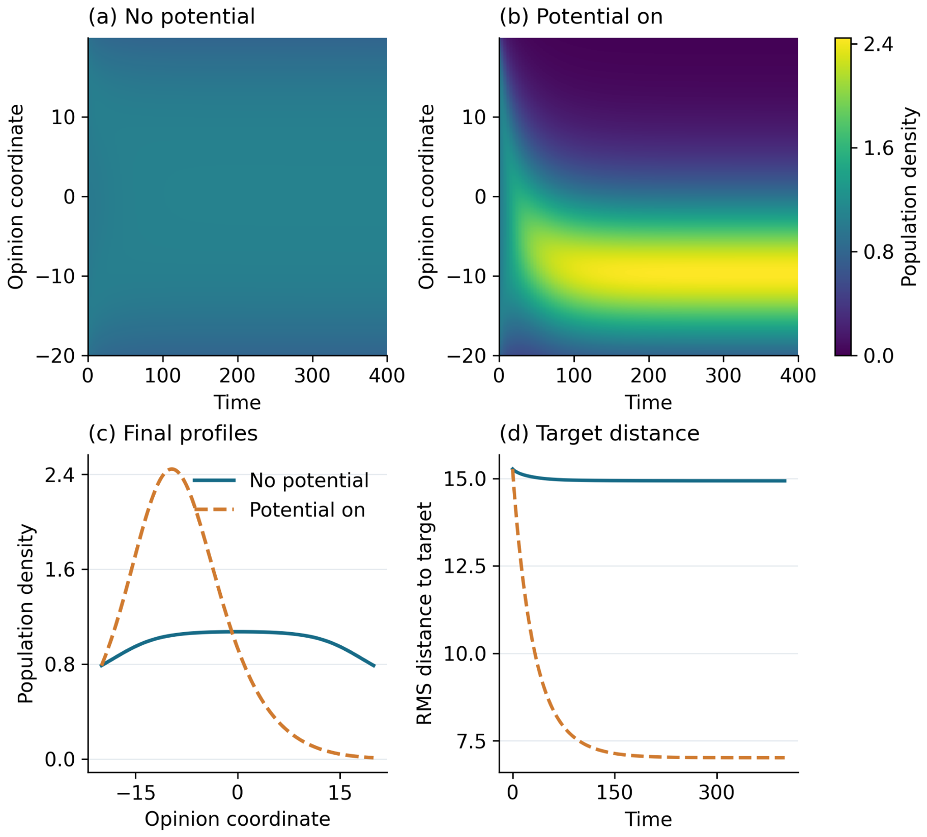
At , the potential run has a density peak at , whereas the control retains a broad profile. Compared with the no-potential control, its population-weighted variance is reduced from to (), and from to (). The maximum recorded relative error in the discrete total population, , is below in both runs. These results support potential-guided redistribution and concentration under the full transport dynamics; they do not isolate the contribution or directly test the homogeneous whole-line reference solution.
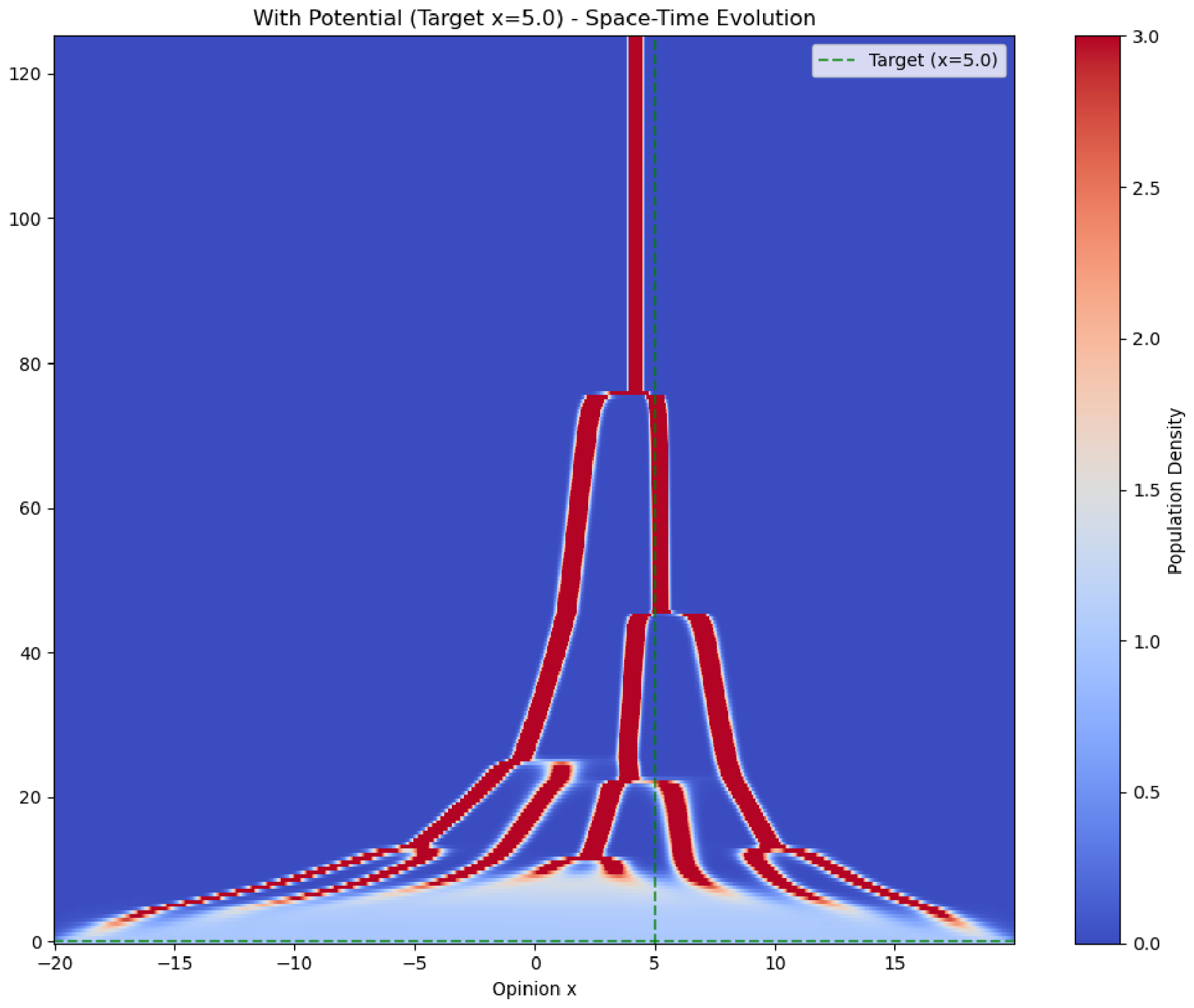
As a further numerical illustration, the parameters , , , , , , , and give the root-like pattern in Figure A2. This pattern is an observation of the simulated dynamics, not a verification of a universal potential-dependent aggregation threshold.
Figure A2.
Root-like opinion aggregation under baseline parameters: , , , , , , , and .
Appendix B. SINP Initialization and Update Formulas
Appendix B.1. SINP Initialization Formula (at Position i)
On the uniform grid with spacing , define the coordinate radius and index radius by
The local index set is
The window is truncated at the endpoints and does not wrap periodically. Initialization applies the following construction to the ordered coordinates and values obtained from and , .
The implementation uses find_peaks with minimum height and minimum separation 10 sample indices. If accepted peaks occur at indices , their mixture weights and means are
Starting from each , the code moves left and right until the first sample at or below half the peak height, or until the corresponding endpoint is reached. Equivalently, the stopping indices are
The discrete width and prescribed component variance are
No crossing interpolation is performed. If a half-height crossing is absent, the width is limited by the window endpoint.
If no peak satisfies the detection criteria, the construction instead sets , , , and , where is the first index attaining . In particular, the no-peak case does not estimate a variance from the width of this maximum. In either case,
Appendix B.2. SINP Update Formula (Given Data Set D)
At an update, the local index set is formed as above using the current global kernel parameters and . Sampling probabilities on this set are proportional to ; if their sum is zero, uniform probabilities are used. The routine draws coordinates with replacement to obtain . This adjustment of sampling weights does not modify the population density used by the PDE solver.
For a nondegenerate sample, the call gaussian_kde(data) uses Scott’s default rule. In the present one-dimensional, equally weighted sample,
where . The symbol denotes the KDE kernel and is distinct from the signed perception kernel and the mixture component count .
The estimate is evaluated at 100 equally spaced coordinates from to , inclusive. The same peak and width construction as in initialization is then applied to these coordinates and KDE values. The peak-height threshold remains , and the minimum separation is 10 KDE evaluation indices, not 10 population-grid intervals. The same single-component, variance- fallback is used if no peak is detected. An empty input sample leaves the existing SINP model unchanged. A successfully constructed mixture replaces the previous one directly; there is no interpolation between old and new mixture parameters, and may change.
Appendix B.3. Core Characteristics
- 1.
- Common construction. Initialization uses population values within each window. Updates use a KDE of locally sampled coordinates. Both use the same peak-height, peak-separation, and discrete-width rules on their respective evaluation grids.
- 2.
- Mixture interpretation. The weights are normalized peak heights, not integrated masses of the surrounding peaks; the means are peak positions. The variance mapping is an algorithmic choice. For an exact Gaussian, the conversion from its full width at half maximum would instead be .
- 3.
- Finite-resolution conventions. The endpoint-limited width, variance floor, and no-peak fallback are explicit implementation conventions. The SINP peak detector described here is distinct from the population-cluster detector used to activate the external potential.
Appendix C. Dataset Header
Table A1.
Dataset features. AST, aspartate aminotransferase; HR, heart rate; RR, respiratory rate; MPV, mean platelet volume; PCT, plateletcrit (thrombocrit); CT, computed tomography; PDW, platelet distribution width; NIV, noninvasive ventilation; MV, mechanical ventilation.
The dataset features are categorized based on their types:
- _stat_control—Static features describing the control process, which do not change over time (in covid_flow, represented as binary features: 1 indicates the drug is included in the treatment plan, and 0 indicates it is not included).
- _dinam_control—Dynamic features describing the control process, which change over time (in covid_flow, represented as binary features: 1 indicates the treatment procedure is included in the treatment plan, 0 indicates not included).
- _stat_fact—Static features describing the controlled process, which do not change over time (in covid_flow, represented as features describing the patient, such as gender, age, and other invariant properties).
- _dinam_fact—Dynamic features describing the controlled process, which change over time (in covid_flow, represented as indicators describing the patient’s state, such as body temperature, percentage of lung infection, etc.).
- Metadata:
- t_point—Time interval identifier. The entire treatment process is divided into equal-length time periods, and t_point is the time period marker.
- Episode-end indicator (end_episode, recorded as end_epizode in the association output): 0 indicates treatment not ended at this t_point, and 1 indicates ended.
- case (index)—Unique identifier for the observation record (treatment process), e.g., “GACAk+Q”.
- long_observation_tar—Total duration of the treatment process.
- current_process_duration—Current treatment duration (up to t_point).
- outcome_tar—Treatment outcome: 1 indicates death, and 0 indicates recovery.
Appendix D. Clinical Data Summaries and Associations
This appendix collects the clinical summaries used to define and interpret the numerical scenarios. The tables report mixture-model profiles, treatment-feature rank changes, period comparisons, and exploratory fact-to-treatment associations.
Table A2.
Top 10 treatment features ranked by mixture-weighted mean propensity within each period, in descending order.
Table A3.
Gaussian Mixture Model results for clinical decision patterns across five periods.
Table A4.
Top 10 treatment features with the largest absolute rank changes from Period 2 to Period 3. Rankings are based on mixture-weighted mean propensity; Δm denotes the later-period value minus the earlier-period value. An upward arrow indicates a move to a smaller rank number, and a downward arrow indicates a move to a larger rank number; the adjacent number is the absolute rank change.
Table A5.
Top 10 treatment features with the largest absolute rank changes from Period 2 to Period 4. Rankings are based on mixture-weighted mean propensity; denotes the later-period value minus the earlier-period value. An upward arrow indicates a move to a smaller rank number, and a downward arrow indicates a move to a larger rank number; the adjacent number is the absolute rank change.
Table A6.
Top 10 treatment features with the largest absolute rank changes from Period 3 to Period 4. Rankings are based on mixture-weighted mean propensity; denotes the later-period value minus the earlier-period value. An upward arrow indicates a move to a smaller rank number, and a downward arrow indicates a move to a larger rank number; the adjacent number is the absolute rank change.
Table A7.
Statistical comparison of medical features between Period 1 and Period 2. AST, aspartate aminotransferase; LDH, lactate dehydrogenase; MPV, mean platelet volume; CT, computed tomography; PDW, platelet distribution width; PCT, plateletcrit (thrombocrit). Sig. (Corr) indicates significance after correction for multiple comparisons.
Table A8.
Statistical comparison of medical features between Period 3 and Period 4. AST, aspartate aminotransferase; LDH, lactate dehydrogenase; MPV, mean platelet volume; CT, computed tomography; PDW, platelet distribution width; PCT, plateletcrit (thrombocrit). Sig. (Corr) indicates significance after correction for multiple comparisons.
Table A9.
Statistical comparison of medical features between Period 2 and Period 3. AST, aspartate aminotransferase; LDH, lactate dehydrogenase; MPV, mean platelet volume; CT, computed tomography; PDW, platelet distribution width; PCT, plateletcrit (thrombocrit). Sig. (Corr) indicates significance after correction for multiple comparisons.
Table A10.
Estimated associations between medical facts and treatment features. DML denotes double machine learning; CI denotes confidence interval. Stars refer to Benjamini–Hochberg-adjusted p-values (q), with adjustment performed separately for each treatment feature: *, ; **, ; and ***, .
Table A11.
All 12 saved prednisolone associations and the seven matched contributions to the fact-informed input S.
Appendix E. Implementation and Checks for the Supplementary Comparisons
Appendix E.1. Implementation Details
The kernel parameters were constrained to and . When , the adaptive scheme proposed an increment of for each parameter, followed by clipping to the bounds. The random scheme proposed independent, equiprobable increments of or for each parameter, without using the target distance. These two schemes shared the same update events and maximum proposed increment per event; their realized cumulative displacements need not be equal. The fixed scheme froze only the kernel parameters and retained the same SINP refresh and distance evaluation procedure. Parameter-update events occurred from to at intervals of ; was an evaluation-only endpoint. At each event, SINP construction and distance evaluation preceded any parameter update, and the updated parameters were used over the next integration interval.
All three schemes used RK23 with relative tolerance , absolute tolerance , and maximum integration step . The nonlocal perceived gradient retained the finite-interval trapezoidal integration convention of the original implementation and was accelerated by an equivalent linear FFT convolution. Diffusion and flux derivatives used differences with periodic indexing. The kernel parameters were updated only at prescribed events and remained fixed within each integration interval. These results therefore constitute a newly computed supplementary comparison under a common protocol; the original single-run distance of was not used as the adaptive reference for this comparison.
Local SINP distributions were constructed by sampling within perception windows with probabilities proportional to the population density, retaining the original KDE, peak-detection, and variance-determination rules. Each local distance estimate used 1000 samples from the SINP distribution and 1000 samples from the target GMM, followed by population-density-weighted aggregation across grid points. For the global distance, grid population densities were normalized to probability masses and compared with 10,000 samples from the target GMM using the Wasserstein distance. Separate random-number streams were used for different sampling purposes and parameter updates; the schemes were paired by seed and used corresponding streams for the same measurement task.
Appendix E.2. Paired Results
Table A12.
Paired endpoint differences in the local perception distance .
Appendix E.3. Parameter Trajectories and Numerical Diagnostics
Table A13.
Parameter-trajectory checks and numerical diagnostics for the original 60-run baseline comparison.
Appendix E.4. Final Densities and Reproducibility Records
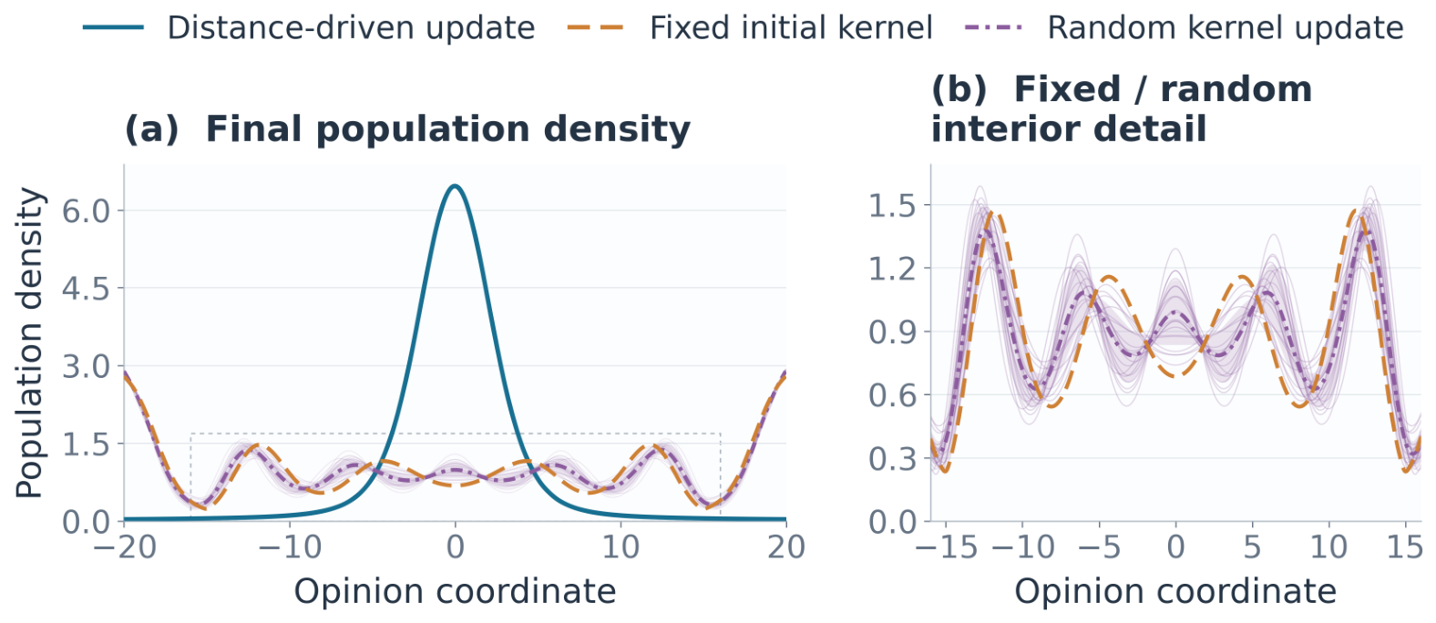
Figure A3 shows the final population densities. The adaptive scheme produced a pronounced central peak near zero, whereas the fixed-initial and random schemes retained more dispersed multiple peaks and higher densities near the domain boundaries. These shapes help interpret the differences in the global distance but do not, by themselves, establish accurate reconstruction of the target distribution.
Figure A3.
Final population densities at . (a) Full-domain comparison of all three schemes. (b) Fixed-initial and random-update controls within , shown on an expanded vertical scale; the dashed rectangle in panel (a) marks the displayed region. Bold curves indicate means. For the random scheme, faint curves show the 20 individual final densities, and shading denotes the mean ± one sample standard deviation. For each of the adaptive and fixed-initial schemes, the final densities coincide across all 20 seeds and are drawn once. All curves use the saved population densities without additional smoothing or normalization to probability densities.
Per-run results, paired differences, complete parameter and density trajectories, the run configuration, and checksums of the experiment code and target file are retained as reproducibility records for this comparison. Selected result tables and the inputs and scripts required to rerun the supplementary experiments are publicly provided; the full collection of saved trajectories is not bundled with the repository.
Appendix E.5. Local Sensitivity and a Fixed-Final-Kernel Control
The supplementary checks retained the preceding target, initial density, parameter bounds, update interval, endpoint , and solver settings. The first 10 original random-seed identifiers, 20260916–20260925, were fixed before running the checks. Four adaptive settings varied one factor at a time, replacing in the proposed increment by : or with , and or with ; throughout. SINP estimates and feedback were recomputed at every event for each seed. Changing d also required recomputing the warm-up from ; changes in reused the original warm-up. The matching 10 original adaptive runs supplied the central reference. For the additional fixed-final control, the kernel was switched to after the evaluation at the first update event, , and then held fixed. Its deterministic density was integrated once and evaluated separately for the 10 seeds. This control permits a direct jump and does not match the per-event increment limit; it is not an optimized fixed kernel. After , its fixed positive kernel and give the continuous equation of Sayama’s fixed-kernel model [15]. The common pre-update density and the present truncated perception integral with periodically indexed differences define our comparison protocol, rather than a reproduction of that paper’s numerical setup.
Table A14.
Supplementary endpoint distances at . Values are means ± sample SD over 10 paired seeds per setting; the central reference reuses the corresponding 10 original runs.
For all listed settings except , the saved parameter and density trajectories coincide across seeds, so distance SDs arise from sampling. At , feedback also introduces small trajectory differences. These are local sensitivity checks, not matched fixed/random-control comparisons at every new setting. At , the final parameters were , and the local distance never fell below 1 by . At , reached its upper bound at , compared with centrally, and both endpoint distances were smaller in all 10 paired comparisons. For , both were larger in all pairs; for , the local distance was smaller in five pairs and larger in five, while the global distance was larger in all ten. The latter setting had 7–10 parameter-changing events per seed with proposed increments below , confirming active distance feedback without isolating its additional performance benefit.
Against the fixed-final control, adaptive updating had a lower mean endpoint local distance, whereas the control had a lower mean global distance; both orderings held in all 10 pairs. The control first attained a local distance below 1 at –, compared with 665– for adaptive updating. Thus, endpoint ordering does not establish an advantage throughout the trajectory or across both metrics. None of the checked settings reached the distance stopping threshold .
Appendix E.6. Numerical Resolution and Discrete Conservation
Numerical checks replayed the exact saved post-event adaptive parameter path, with no SINP feedback recalculation. The original 1000-point run used relative/absolute tolerances ; three additional runs used 500, 1000, and 2000 points with . Each new discretization recomputed the warm-up from the same analytic initial density. All runs retained the same finite-interval trapezoidal rule for the nonlocal integral and periodic-index differences for diffusion and flux derivatives. The global distances, including the original reference, were re-evaluated using one common set of 10,000 target samples, removing target-sampling differences from the numerical comparison. The endpoint values are listed in Table A15.
Table A15.
Endpoint global distances under the same prescribed parameter path and common target sample. The standard-tolerance 1000-point density is reused; the other three settings are new runs.
At 1000 points, tightening the tolerances changed the endpoint global distance by ; the largest absolute difference over all 1102 saved times was . For the 500–1000 and 1000–2000 pairs at tight tolerances, endpoint absolute differences were and ( and of the finer-grid values). Their maximum relative differences over saved times were and , respectively. The latter occurred at , rather than at the endpoint. The endpoint density-to-density values were and ; thus, adjacent-grid differences decreased by approximately a factor of two. Density-to-density distances also include differences in discrete grid support. These checks quantify resolution dependence for the prescribed path, not convergence of the full stochastic feedback algorithm; the finest grid is a comparison reference, not a known exact solution.
For these potential-free comparisons, the semi-discrete mass is . With and periodic indices,
Parameter updates do not change the density state. Across the 50 additional seed-specific records and the three numerical replays, the smallest saved density was , and the maximum recorded relative mass error was approximately . These are diagnostics at saved times, not continuous-time nonnegativity guarantees. Detailed configurations, individual trajectories, paired results, common target samples, and code checksums are retained with the supplementary records.
The public baseline and additional-check runners are r1_3_baseline_experiment.py and r2_4_supplementary_experiments.py, respectively. The public baseline reads azithromycin_period3_target.json, which preserves the selected marginal parameters used in the original run, and records its target and configuration in config_and_target.json. The additional runner requires a completed formal 20-seed baseline and documents its reuse in manifest.json. The outputs summary.csv, paired_summary.csv, and numerical_comparisons.csv provide the corresponding endpoint, paired, and numerical comparisons. The recorded environment was Python 3.12.2, NumPy 1.26.4, and SciPy 1.14.1. The public input adapters retain the original numerical conventions; repository details are provided in the Data Availability Statement.
Appendix F. Boundary and Domain Sensitivity of Experiment 3
Appendix F.1. Controlled Continuation Protocol
Four potential-free continuations start from the same archived Experiment 3 density , with , , and . The original grid is , . All runs use the same prescribed parameter path,
where are the archived terminal parameters, used at their stored precision. The density is unchanged at the parameter switch. This controlled two-stage protocol is not an exact replay of the original updates within adaptive solver evaluations. No SINP or target-distance feedback is performed in these checks.
The four settings are:
- 1.
- Mixed, : The original combination of finite-interval trapezoidal quadrature for the nonlocal perception and periodic-index differences for the differential flux.
- 2.
- No flux, : The same truncated perception integral and interior difference stencil, with zero total flux at both outer faces. With the sampling points treated as equal-width cell centers, these faces are at and .
- 3.
- Periodic, : A periodized perception kernel with periodic rectangle quadrature and the same periodic differential stencil.
- 4.
- Mixed, : The mixed treatment on 2000 points, , . The initial density is extended by zero, retaining the original grid values, spacing, and total population.
All runs use RK23 with relative tolerance , absolute tolerance , and maximum time step . Each run saves 451 density states at intervals of two time units over . The shared initial state retains the original pre-700 history; the checks therefore concern the continuation stage. Domain extension also changes the accessible space and mean density, rather than only the endpoint condition.
Appendix F.2. Reference Agreement and Boundary Comparisons
At , the controlled mixed reference reproduces the archived three-peak structure at . Its normalized-density from the archived endpoint is , and its relative density difference is . The trajectories are not identical: comparison with the time-interpolated archive gives a maximum relative difference of approximately during the stage transition. The agreement supports its use as a controlled reference for the late-stage pattern.
Table A16 summarizes the endpoint comparisons. Here, compares normalized grid population masses with those of the controlled mixed reference. It is the ordinary one-dimensional distance on the displayed real coordinate, not a circular Wasserstein distance or a SINP-to-clinical-target discrepancy. Peak detection uses a height threshold of and a minimum separation of two coordinate units, counting a periodic seam peak once.
Table A16.
Boundary and domain comparisons at . Listed peak positions satisfy the prescribed height and separation criteria. Distances compare each normalized population distribution with the controlled mixed reference at .
The no-flux result remains close to the mixed reference throughout the saved interval: its maximum is . The two outer peaks lie approximately coordinate units from the end faces. Thus, replacing the periodic endpoint connection of the differential flux has little effect in this continuation. Both runs nevertheless retain the same truncated perception integral, so this agreement does not exclude effects of that truncation.
The fully periodic run instead produces four detected peaks, including one peak across the periodic seam at . The extended-domain run has four above-threshold peaks and two additional lower peripheral peaks at and , each with height approximately . Its population mass outside the original interval is , or of the total. This is redistribution into the extended region, not population loss. Figure A4 shows the endpoint profiles, including the lower peripheral peaks.
Figure A4.
Saved population densities at : (a) full sampled domains; (b) the common central interval. The archived endpoint, controlled mixed reference, and no-flux profile overlap closely. The two ends of the periodic curve represent a single seam peak.
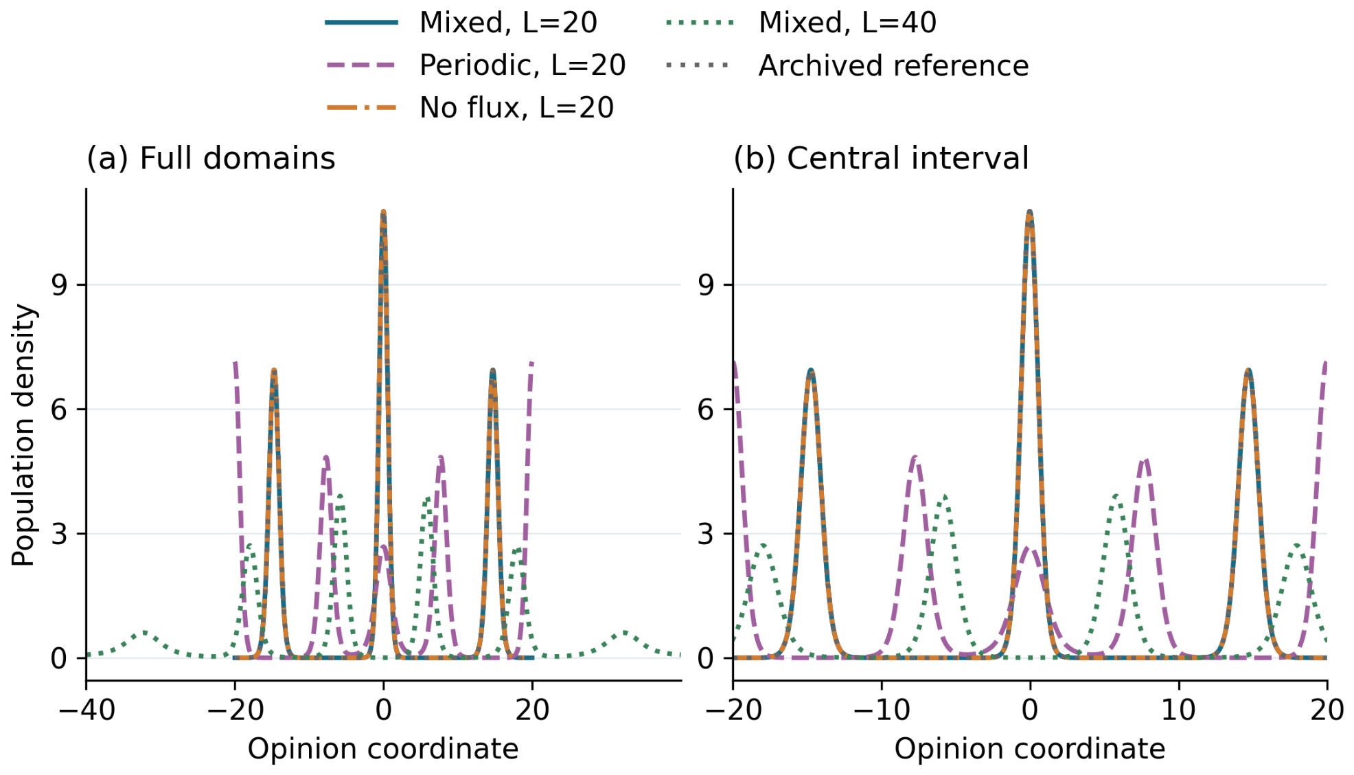
Appendix F.3. Late-Time Evolution and Numerical Diagnostics
Figure A5 shows that the periodic and extended-domain patterns continue to evolve near the endpoint. The relative change
is approximately for both the mixed and no-flux runs, compared with for the periodic run and for the extended-domain run. These values measure density differences, not the fraction of individuals that migrated. The latter two endpoints should therefore not be interpreted as established stationary states.
Across all four runs, the maximum recorded relative error in is below . All saved densities on the original domain are positive. The extended-domain run has a minimum saved value of in the initially empty region, consistent with roundoff-scale negativity. The PDE states are neither clipped nor renormalized; roundoff-scale negative values are removed only when constructing probability masses for evaluation. These diagnostics do not constitute a continuous-time nonnegativity proof.
Overall, the original three-peak structure is preserved under the tested no-flux replacement, and all four settings show multiple peaks at . The precise peak count, locations, and evolution depend on the perception boundary treatment and domain setting. The checks do not establish boundary-independent three-peak selection or remove the boundary history inherited by .
The checks are run by r3_4_exp3_boundary_sensitivity.py, using r3_4_experiment_core.py. Configurations, source and code checksums, saved densities, and diagnostics are retained with the supplementary records. The files case_summary.csv, comparisons.csv, and controlled_reference_vs_original.csv document the case summaries and comparisons.
Figure A5.
Density evolution under the common prescribed parameter path: (a) mixed, ; (b) periodic, ; (c) no flux, ; (d) mixed, . All panels use a common density color scale; panel (d) shows the full extended domain.
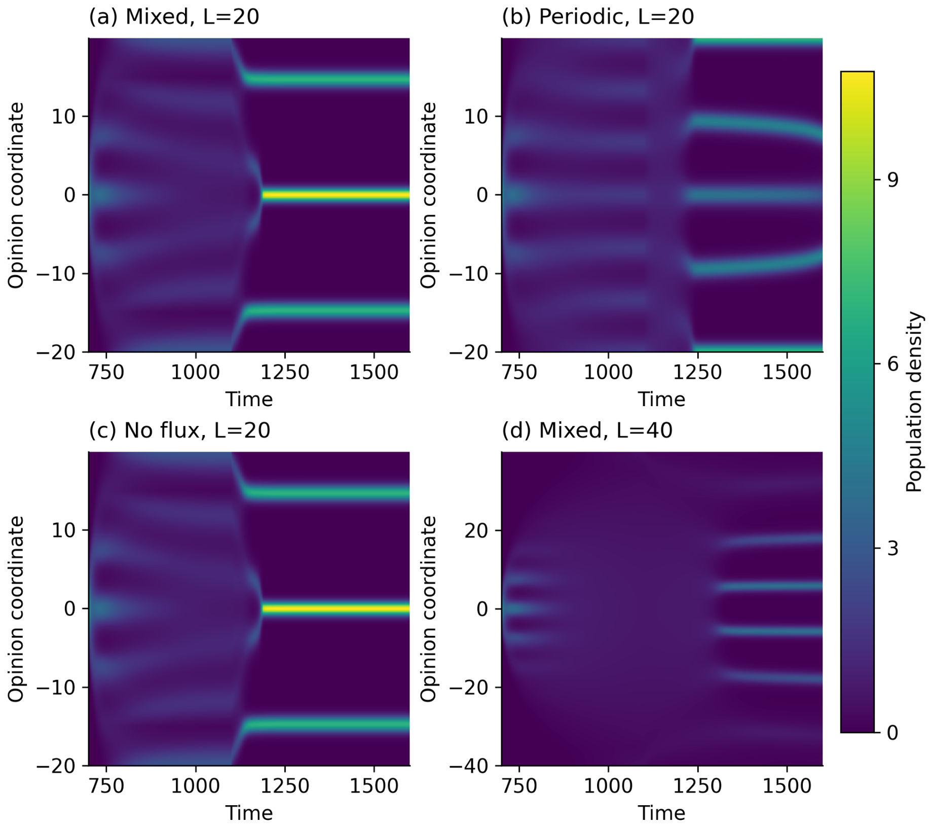
Appendix G. Primary Experiment Settings and Saved-State Diagnostics
Table A17 and Table A18 summarize the original three experiments. These settings are separate from the event-based supplementary controls in Appendix E and the controlled boundary continuations in Appendix F.
Table A17.
Common settings of the three primary experiments.
Table A18.
Targets, stages, and potential rules in the primary experiments.
The distance threshold applies to the target-driven update, not to the later fact-informed stages. Those stages use the common base input S with the gradient and elapsed-call-time factors specified in Section 5.2; clipping may make the two realized parameter increments different.
For each saved density, the discrete mass is . Table A19 reports and the minimum density over the saved spatial and temporal grids. The results support conservation of total population in the saved computations; local density reductions represent redistribution. These checks do not establish nonnegativity at every internal solver evaluation or a general positivity-preserving property of the numerical method.
Table A19.
Diagnostics from the archived primary-experiment densities.
Appendix H. Conditional Properties of the Continuous Model
This appendix concerns explicitly specified continuous boundary-value problems. These statements are separate from the whole-line linear reference in Appendix A and from the properties of the discrete solvers.
Appendix H.1. Fixed-Parameter Evolution with Zero Total Flux
Let , , and define the truncated operator
The continuous problem considered here is
The boundary condition specifies zero total flux, not .
Proposition A1 (Fixed-parameter evolution).
Let , let g be smooth on a neighborhood of , and let V be smooth on ; both are time-independent. Suppose for some , , , and at both endpoints. Then, Equation (A11) has a unique global classical solution, continuous to and classical for . It conserves mass M, is strictly positive for positive times, and depends continuously in on admissible initial data on finite time intervals. These assumptions hold for the spatial coefficients of the fixed signed Gaussian kernel in Equation (3) and a fixed quadratic potential; the initial and boundary conditions remain separate requirements.
Proof.
Set . Zero total flux gives , , and
Conversely, differentiation of this Dirichlet problem gives Equation (A11) for . Write , where and v has zero endpoint values. The map is locally Lipschitz from functions with zero endpoint values to . If denotes the Dirichlet heat semigroup, its gradient estimate for makes
a contraction on a suitable ball in with zero endpoint values when is small, since . Smooth coefficients give classical regularity for positive times; the stated compatibility condition handles the initial boundary.
For this local solution, the maximum principle applied to Equation (A12) yields . Let , , and . Then,
For every finite T, the mild equation gives, while the solution exists,
The fractional Gronwall inequality bounds this norm on every finite time interval. Together with , this excludes the blow-up alternative for the local construction and gives global continuation. Parabolic regularity gives the asserted regularity of for .
To verify nonnegativity without assuming it in the construction, let . The zero-flux boundary condition yields
Since , Gronwall’s inequality gives . Integration of the equation gives . Consequently, with , testing the equation with P gives the further estimate
For the resulting solution, the drift and its spatial derivative are bounded on finite time intervals. After multiplying P by with C chosen to make the zeroth-order coefficient nonnegative, the strong minimum principle applied with this drift fixed gives positivity in the interior for . A zero at an endpoint would imply there by the zero-flux condition, contradicting the boundary point lemma for a nonzero nonnegative solution. Thus, positivity also holds at the endpoints for .
For uniqueness, let be two such solutions and set . Linearity of gives
Testing the difference equation by Z and using the zero-flux conditions and Young’s inequality gives
on every finite interval, with finite by the preceding bounds. Gronwall’s inequality gives . The preceding mass and bounds control on bounded sets of admissible initial data. This proves continuous dependence and, for equal initial data, uniqueness. □
Relation to the Periodic Theory
For a separate periodic formulation of length L, periodize the averaging kernel from Section 3 as , where and . For fixed parameters and , set . The periodic equation becomes
where ∗ is periodic convolution. The smooth even potential W satisfies Assumption (A1) of the cited paper by Carrillo et al. [54]. For nonnegative, unit-mass periodic initial data in one dimension, Theorem 2.2 of Carrillo et al. [54] applies with and , giving a unique classical solution, strict positivity, and finite entropy for . This is a periodic reference result, not a direct application to the zero-flux problem above or to the mixed numerical boundary treatment. The periodic regularity of the initial data is an additional assumption. In particular, the 40-periodic extension of the simulation initial profile has mismatched endpoint values and does not satisfy the stated condition.
Appendix H.2. Free-Energy Dissipation for Fixed Parameters
Proposition A2 (Fixed-parameter dissipation).
For the solution of Proposition A1 with this kernel and fixed V, define
with at . Then, for ,
The energy has a finite limit as , and the total dissipation is finite on for every .
Proof.
Symmetry of w gives . The equation is and . Integration by parts, using at both endpoints, proves Equation (A14). Jensen’s inequality and conservation of mass give the lower bound
Monotonicity and this bound give the finite energy limit and, by integrating Equation (A14), finite total dissipation after any positive time. □
This result establishes a dissipative structure for the fixed-parameter continuous problem. It does not establish uniqueness of an equilibrium, convergence of the density to a particular equilibrium or clinical target, or monotonicity of either reported Wasserstein metric. Time-dependent kernels and potentials add terms to the energy balance; parameter jumps can also change the energy. A single globally decreasing energy is therefore not asserted for the feedback system.
Appendix H.3. Prescribed Update Events and Scope
At a prescribed sequence of update times with finitely many events in each finite time interval, the continuous evolution can be constructed successively between events. Conditional on a fixed realization of the random inputs, assume every update is a single-valued, fully defined function of the current state and stored history, leaves P unchanged, and selects smooth spatial coefficients within fixed bounds, including . Each interval then has a unique evolution with its selected fixed coefficients. For zero-flux boundaries, a parameter change may destroy classical compatibility at the event itself. Restart the cumulative Dirichlet problem in the mild sense from the continuous density; the same local construction and bounds apply, and the new zero-flux condition and classical regularity hold for times strictly after the event. Induction gives a unique path for this specified event-driven continuous model. It does not imply continuous dependence across discontinuous update rules or equality of paths for different random inputs.
This construction clarifies the mathematical interpretation of prescribed update events; it is not a convergence or positivity proof for their numerical discretization. In particular, the primary notebooks update parameters during BDF right-hand-side evaluations, whereas the additional Experiment 1 comparison protocol described in Appendix E uses prescribed external events. The original mixed treatment combines truncated perception with periodically indexed differences and is not identified with either continuous boundary-value problem proved here. The separate numerical diagnostics and limitations in Appendix E, Appendix F and Appendix G remain applicable.
References
- Donaldson, T.; Dunfee, T.W. Toward A Unified Conception Of Business Ethics: Integrative Social Contracts Theory. Acad. Manag. Rev. 1994, 19, 252–284. [Google Scholar] [CrossRef] [Scilit]
- Goldstein, N.J.; Cialdini, R.B. Using Social Norms as a Lever of Social Influence. In The Science of Social Influence: Advances and Future Progress; Pratkanis, A.R., Ed.; Psychology Press: Philadelphia, PA, USA, 2007; pp. 167–192. [Google Scholar]
- Morris, M.W.; Hong, Y.Y.; Chiu, C.Y.; Liu, Z. Normology: Integrating insights about social norms to understand cultural dynamics. Organ. Behav. Hum. Decis. Processes 2015, 129, 1–13. [Google Scholar] [CrossRef] [Scilit]
- Scharding, T.K.; Warren, D.E. When Are Norms Prescriptive? Understanding and Clarifying the Role of Norms in Behavioral Ethics Research. Bus. Ethics Q. 2023, 34, 331–364. [Google Scholar] [CrossRef] [Scilit]
- Kalantari, S.A.; Luntley, M. On the logic of aiming at truth. Analysis 2013, 73, 419–422. [Google Scholar] [CrossRef] [Scilit]
- Kasper, S.; Cubała, W.J.; Fagiolini, A.; Ramos-Quiroga, J.A.; Souery, D.; Young, A.H. Practical recommendations for the management of treatment-resistant depression with esketamine nasal spray therapy: Basic science, evidence-based knowledge and expert guidance. World J. Biol. Psychiatry 2020, 22, 468–482. [Google Scholar] [CrossRef] [Scilit]
- Phi, L.; Ajaj, R.; Ramchandani, M.H.; Brant, X.M.; Oluwadara, O.; Polinovsky, O.; Moradi, D.R.; Barkhordarian, A.; Sriphanlop, P.; Ong, M.; et al. Expanding the Grading of Recommendations Assessment, Development, and Evaluation (Ex-GRADE) for Evidence-Based Clinical Recommendations: Validation Study. Open Dent. J. 2012, 6, 31–40. [Google Scholar] [CrossRef] [Scilit]
- Chen, Y.; Bosse, T.; Woensdregt, M. Social norms as an interactive process: An agent-based cognitive modelling study. In Proceedings of the Annual Meeting of the Cognitive Science Society, Rotterdam, The Netherlands, 24–27 July 2024; Volume 46. [Google Scholar]
- Mogilner, A.; Edelstein-Keshet, L. A non-local model for a swarm. J. Math. Biol. 1999, 38, 534–570. [Google Scholar] [CrossRef] [Scilit]
- Keller, E.F.; Segel, L.A. Initiation of slime mold aggregation viewed as an instability. J. Theor. Biol. 1970, 26, 399–415. [Google Scholar] [CrossRef] [Scilit]
- Horstmann, D. From 1970 until Present: The Keller–Segel Model in Chemotaxis and Its Consequences. I. Jahresber. Dtsch. Math.-Ver. 2003, 105, 103–165. [Google Scholar]
- Boi, S.; Capasso, V.; Morale, D. Modeling the aggregative behavior of ants of the species Polyergus rufescens. Nonlinear Anal. Real World Appl. 2000, 1, 163–176. [Google Scholar] [CrossRef] [Scilit]
- Hillen, T.; Painter, K.J. A user’s guide to PDE models for chemotaxis. J. Math. Biol. 2009, 58, 183–217. [Google Scholar] [CrossRef] [Scilit]
- Di Francesco, M.; Fagioli, S. Measure solutions for non-local interaction PDEs with two species. Nonlinearity 2013, 26, 2777. [Google Scholar] [CrossRef] [Scilit]
- Sayama, H. Enhanced ability of information gathering may intensify disagreement among groups. Phys. Rev. E 2020, 102, 012303. [Google Scholar] [CrossRef] [Scilit]
- Tan, Z.X.; Brawer, J.; Scassellati, B. That’s Mine! Learning Ownership Relations and Norms for Robots. In Proceedings of the Thirty-Third AAAI Conference on Artificial Intelligence, Honolulu, HI, USA, 27 January–1 February 2019; Volume 33, pp. 8058–8065. [Google Scholar] [CrossRef] [Scilit]
- Cranefield, S.; Meneguzzi, F.; Oren, N.; Savarimuthu, B.T.R. A Bayesian Approach to Norm Identification. In Proceedings of the 22nd European Conference on Artificial Intelligence, The Hague, The Netherlands, 29 August–2 September 2016; pp. 622–629. [Google Scholar] [CrossRef] [Scilit]
- Nichols, S.; Kumar, S.; Lopez, T.; Ayars, A.; Chan, H. Rational Learners and Moral Rules. Mind Lang. 2016, 31, 530–554. [Google Scholar] [CrossRef] [Scilit]
- Han, L.; Wu, F. COVID-19 drives medical education reform to promote “healthy China 2030” action plan. Front. Public Health 2024, 12, 1465781. [Google Scholar] [CrossRef] [Scilit]
- Chen, S.Y.; Lo, H.Y.; Hung, S.K. What is the impact of the COVID-19 pandemic on residency training: A systematic review and analysis. BMC Med. Educ. 2021, 21, 618. [Google Scholar] [CrossRef] [Scilit]
- Oldenburg, N.; Tan, Z.X. Learning and Sustaining Shared Normative Systems via Bayesian Rule Induction in Markov Games. arXiv 2024, arXiv:2402.13399. [Google Scholar]
- Axelrod, R.; Hamilton, W.D. The evolution of cooperation. Science 1981, 211, 1390–1396. [Google Scholar] [CrossRef] [Scilit]
- Savarimuthu, B.T.R.; Cranefield, S.; Purvis, M.K.; Purvis, M.A. Norm emergence in agent societies formed by dynamically changing networks. Web Intell. Agent Syst. 2009, 7, 223–232. [Google Scholar] [CrossRef] [Scilit]
- Vinitsky, E.; Köster, R.; Agapiou, J.P.; Duéñez-Guzmán, E.A.; Vezhnevets, A.S.; Leibo, J.Z. A learning agent that acquires social norms from public sanctions in decentralized multi-agent settings. Collect. Intell. 2023, 2, 26339137231162025. [Google Scholar] [CrossRef] [Scilit]
- Cushman, F.; Sarin, A.; Ho, M. Punishment as Communication. In The Oxford Handbook of Moral Psychology; Vargas, M., Doris, J.M., Eds.; Oxford University Press: Oxford, UK, 2022; pp. 197–209. [Google Scholar] [CrossRef] [Scilit]
- Yan, E.; Nardin, L.G.; Hübner, J.F.; Boissier, O. An agent-centric perspective on norm enforcement and sanctions. In Coordination, Organizations, Institutions, Norms, and Ethics for Governance of Multi-Agent Systems XVII; Cranefield, S., Nardin, L.G., Lloyd, N., Eds.; Springer: Cham, Switzerland, 2025; Volume 15398, pp. 79–99. [Google Scholar] [CrossRef] [Scilit]
- Leibo, J.Z.; Dueñez-Guzman, E.A.; Vezhnevets, A.; Agapiou, J.P.; Sunehag, P.; Koster, R.; Matyas, J.; Beattie, C.; Mordatch, I.; Graepel, T. Scalable evaluation of multi-agent reinforcement learning with melting pot. In Proceedings of the International Conference on Machine Learning, PMLR, Virtual, 18–24 July 2021; pp. 6187–6199. [Google Scholar]
- Agapiou, J.P.; Vezhnevets, A.S.; Duéñez-Guzmán, E.A.; Matyas, J.; Mao, Y.; Sunehag, P.; Köster, R.; Madhushani, U.; Kopparapu, K.; Comanescu, R.; et al. Melting Pot 2.0. arXiv 2022, arXiv:2211.13746. [Google Scholar]
- Tan, Z.X.; Ong, D.C. Bayesian inference of social norms as shared constraints on behavior. arXiv 2019, arXiv:1905.11110. [Google Scholar]
- Theriault, J.E.; Young, L.; Barrett, L.F. The sense of should: A biologically-based framework for modeling social pressure. Phys. Life Rev. 2019, 36, 100–136. [Google Scholar] [CrossRef] [Scilit]
- Kelly, D.; Davis, T. SOCIAL NORMS AND HUMAN NORMATIVE PSYCHOLOGY. Soc. Philos. Policy 2018, 35, 54–76. [Google Scholar] [CrossRef] [Scilit]
- Dingemanse, M.; Liesenfeld, A.; Rasenberg, M.; Albert, S.; Ameka, F.K.; Birhane, A.; Bolis, D.; Cassell, J.; Clift, R.; Cuffari, E.C.; et al. Beyond Single-Mindedness: A Figure-Ground Reversal for the Cognitive Sciences. Cogn. Sci. 2023, 47, e13230. [Google Scholar] [CrossRef] [Scilit]
- Mirski, R.; Bickhard, M.H. Conventional minds: An interactivist perspective on social cognition and its enculturation. New Ideas Psychol. 2021, 62, 100856. [Google Scholar] [CrossRef] [Scilit]
- Shum, M.; Kleiman-Weiner, M.; Littman, M.L.; Tenenbaum, J.B. Theory of minds: Understanding behavior in groups through inverse planning. In Proceedings of the AAAI Conference on Artificial Intelligence, Honolulu, HI, USA, 27 January–1 February 2019; Volume 33, pp. 6163–6170. [Google Scholar]
- Galinsky, A.; Schweitzer, M. Friend and Foe: When to Cooperate, When to Compete, and How to Succeed at Both; Random House Business: London, UK, 2016. [Google Scholar]
- Ong, D.C.; Zaki, J.; Goodman, N.D. Affective cognition: Exploring lay theories of emotion. Cognition 2015, 143, 141–162. [Google Scholar] [CrossRef] [Scilit]
- Wu, Y.; Baker, C.L.; Tenenbaum, J.B.; Schulz, L.E. Rational inference of beliefs and desires from emotional expressions. Cogn. Sci. 2018, 42, 850–884. [Google Scholar] [CrossRef] [Scilit]
- Jara-Ettinger, J.; Gweon, H.; Schulz, L.E.; Tenenbaum, J.B. The naïve utility calculus: Computational principles underlying commonsense psychology. Trends Cogn. Sci. 2016, 20, 589–604. [Google Scholar] [CrossRef] [Scilit]
- Li, C.; Petruchik, O.; Grishanina, E.; Kovalchuk, S. Multi-agent norm perception and induction in distributed healthcare. J. Biomed. Inform. 2025, 166, 104835. [Google Scholar] [CrossRef] [Scilit]
- Li, C.; Petruchik, O.; Kovalchuk, S. Modeling Medical Descriptive Norm Convergence and Violation via Nonlocal Transport and Agent Learning. In Proceedings of the 18th International Conference on Agents and Artificial Intelligence (ICAART 2026); SCITEPRESS: Setubal, Portugal, 2026; Volume 3, pp. 2308–2315. [Google Scholar] [CrossRef] [Scilit]
- Bakshy, E.; Messing, S.; Adamic, L.A. Exposure to ideologically diverse news and opinion on Facebook. Science 2015, 348, 1130–1132. [Google Scholar] [CrossRef] [Scilit]
- Kwon, J.; Tan, Z.-X.; Tenenbaum, J.; Levine, S. When It Is Not Out of Line to Get Out of Line: The Role of Universalization and Outcome-Based Reasoning in Rule-Breaking Judgments. PsyArXiv 2023. preprint. [Google Scholar] [CrossRef] [Scilit]
- Levine, S.; Kleiman-Weiner, M.; Schulz, L.; Tenenbaum, J.; Cushman, F. The logic of universalization guides moral judgment. Proc. Natl. Acad. Sci. USA 2020, 117, 26158–26169. [Google Scholar] [CrossRef] [Scilit]
- Huber, M.; Hsu, Y.C.; Lee, Y.Y.; Lettry, L. Direct and indirect effects of continuous treatments based on generalized propensity score weighting. J. Appl. Econom. 2020, 35, 814–840. [Google Scholar] [CrossRef] [Scilit]
- Brown, D.W.; Greene, T.J.; Swartz, M.D.; Wilkinson, A.V.; DeSantis, S.M. Propensity score stratification methods for continuous treatments. Stat. Med. 2021, 40, 1189–1203. [Google Scholar] [CrossRef] [Scilit]
- Austin, P.C. Assessing covariate balance when using the generalized propensity score with quantitative or continuous exposures. Stat. Methods Med. Res. 2019, 28, 1365–1377. [Google Scholar] [CrossRef] [Scilit]
- Staw, B.M.; Sandelands, L.E.; Dutton, J.E. Threat rigidity effects in organizational behavior: A multilevel analysis. Adm. Sci. Q. 1981, 26, 501–524. [Google Scholar] [CrossRef] [Scilit]
- Weick, K.E. Enacted Sensemaking in Crisis Situations. J. Manag. Stud. 1988, 25, 305–317. [Google Scholar] [CrossRef] [Scilit]
- Weick, K.E. The vulnerable system: An analysis of the Tenerife air disaster. J. Manag. 1990, 16, 571–593. [Google Scholar] [CrossRef] [Scilit]
- Beach, L.R.; Mitchell, T.R. A contingency model for the selection of decision strategies. Acad. Manag. Rev. 1978, 3, 439–449. [Google Scholar] [CrossRef] [Scilit]
- Sayama, H. Introduction to the Modeling and Analysis of Complex Systems; Open SUNY Textbooks: Geneseo, NY, USA, 2015. [Google Scholar]
- Morris-Martin, A.; De Vos, M.; Padget, J. Norm emergence in multiagent systems: A viewpoint paper. Auton. Agents Multi-Agent Syst. 2019, 33, 706–749. [Google Scholar] [CrossRef] [Scilit]
- Li, X.; Wang, S.; Zeng, S.; Wu, Y.; Yang, Y. A survey on LLM-based multi-agent systems: Workflow, infrastructure, and challenges. Vicinagearth 2024, 1, 9. [Google Scholar] [CrossRef] [Scilit]
- Carrillo, J.A.; Gvalani, R.S.; Pavliotis, G.A.; Schlichting, A. Long-Time Behaviour and Phase Transitions for the McKean–Vlasov Equation on the Torus. Arch. Ration. Mech. Anal. 2020, 235, 635–690. [Google Scholar] [CrossRef] [Scilit]
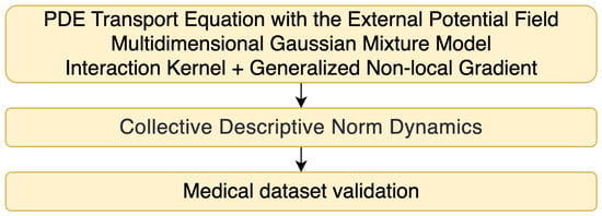
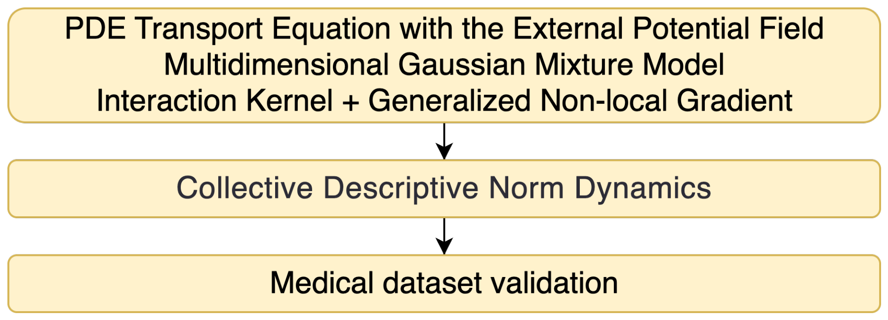
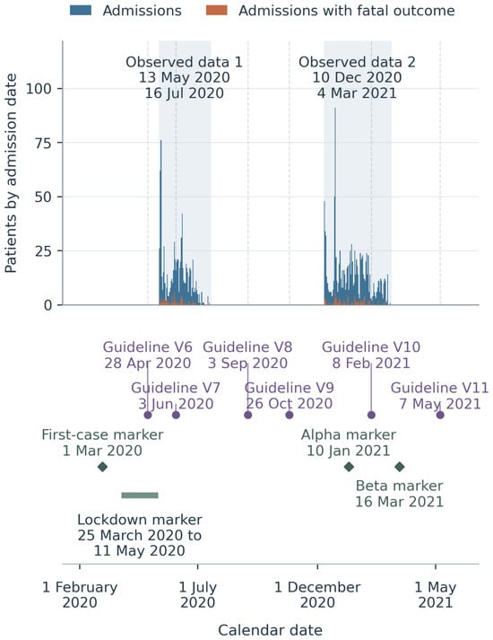
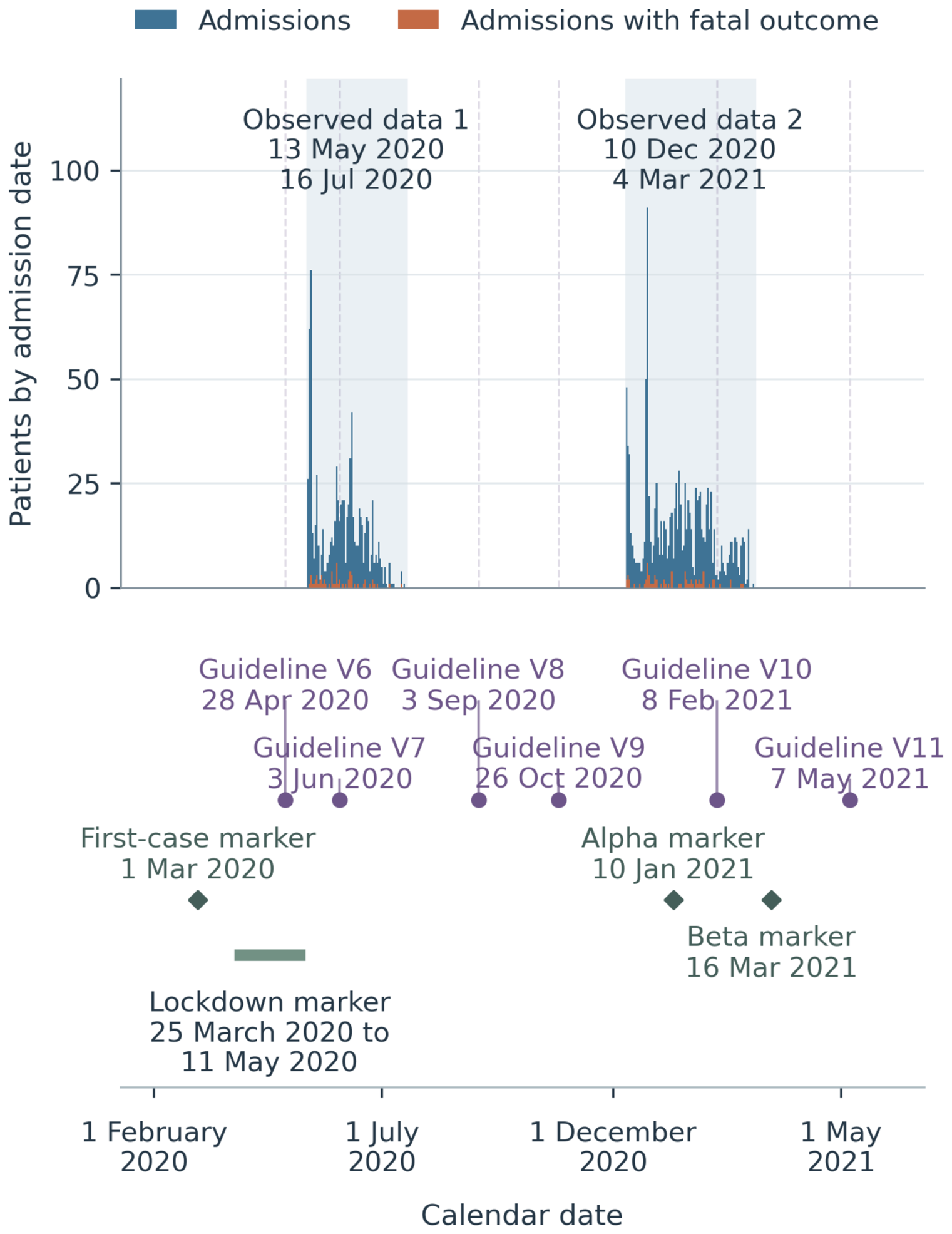
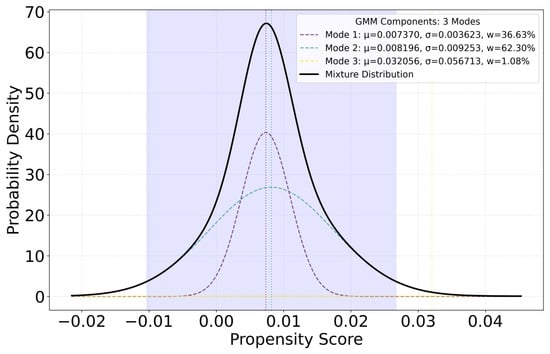
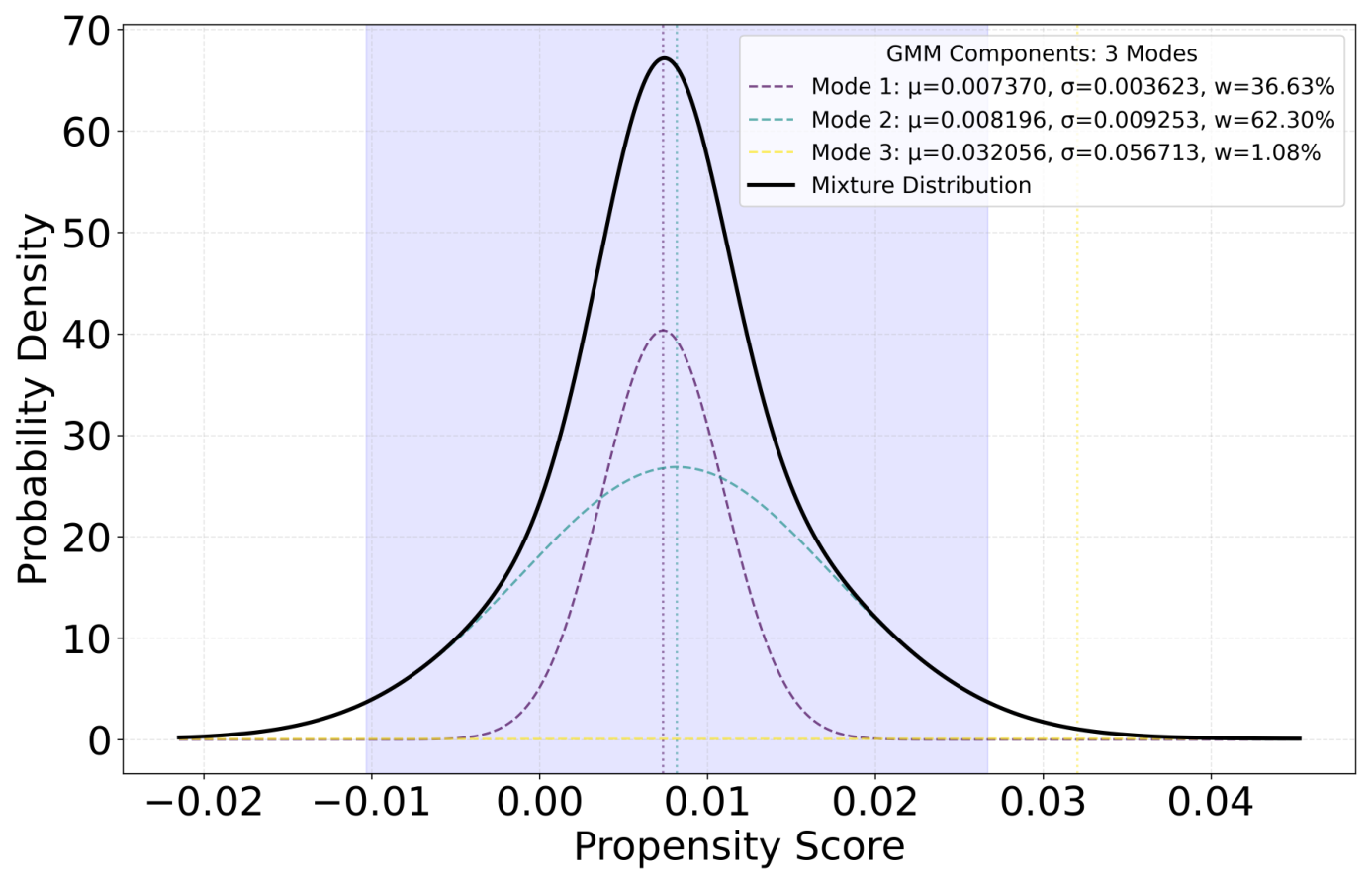
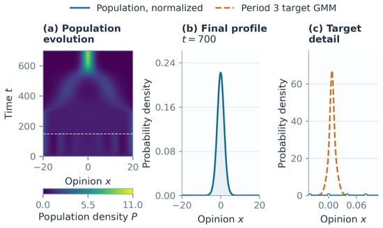
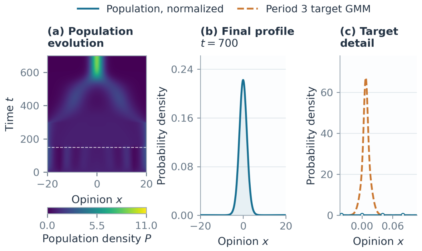
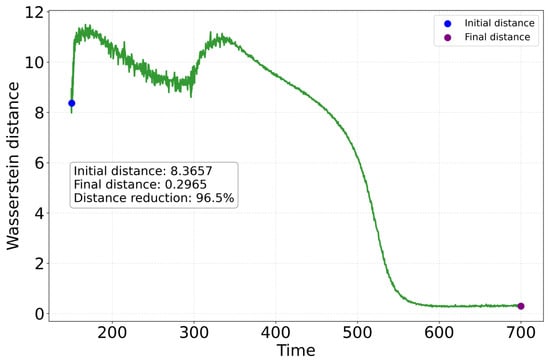
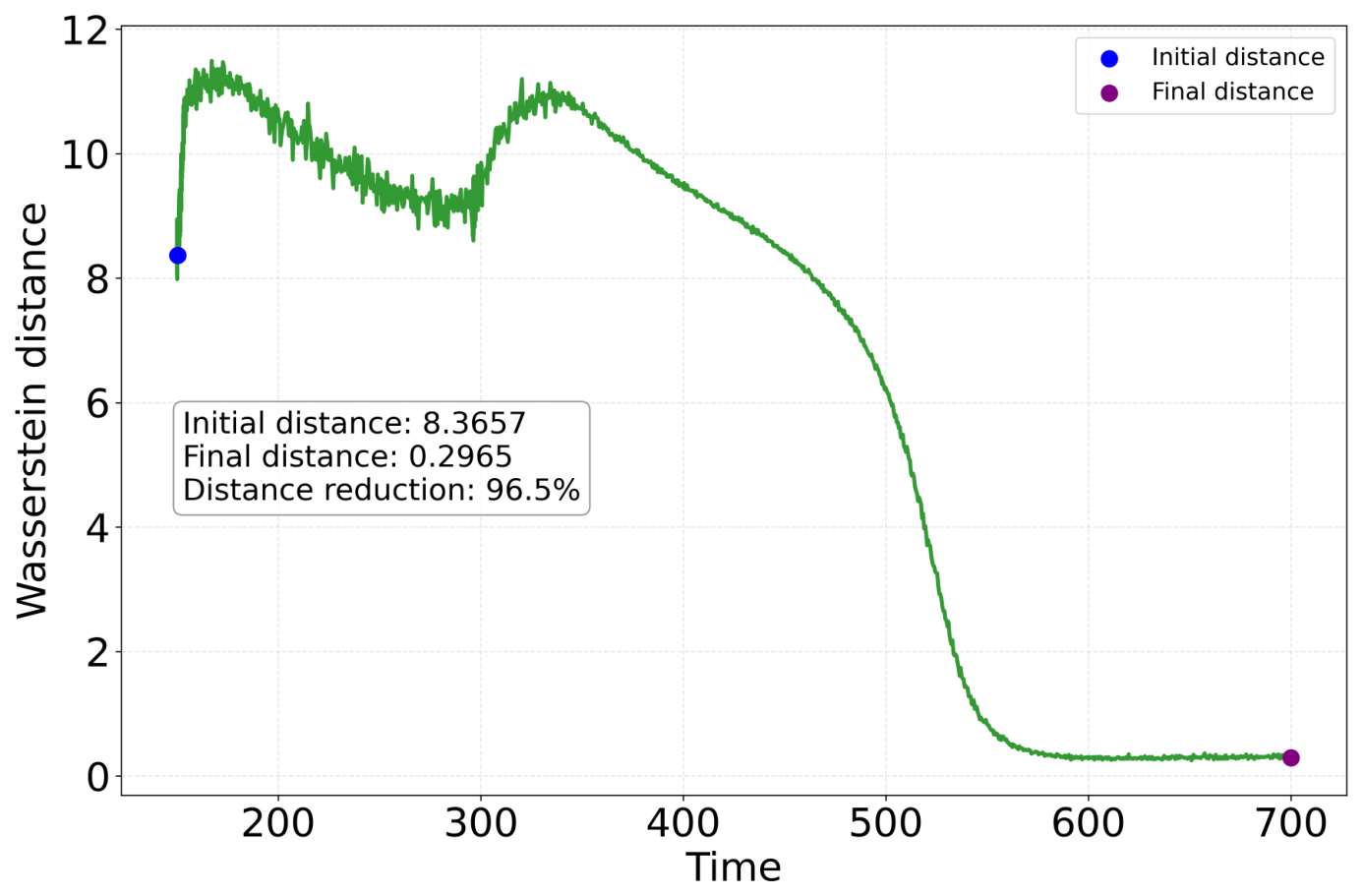
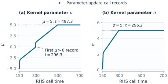
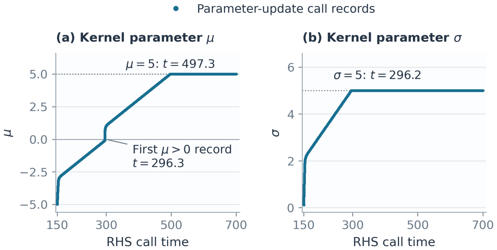
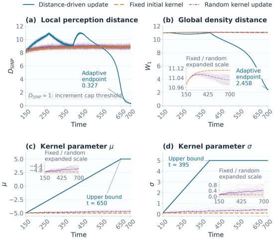
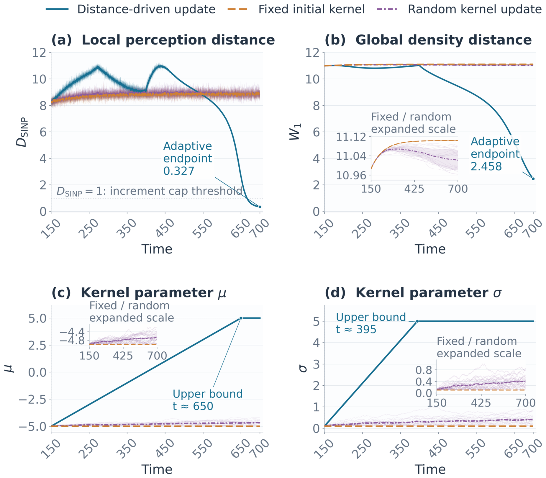
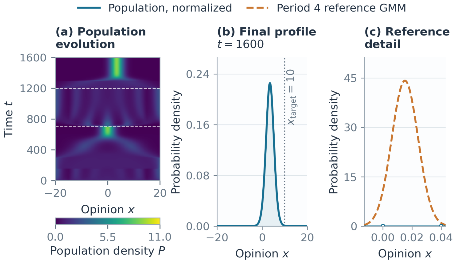
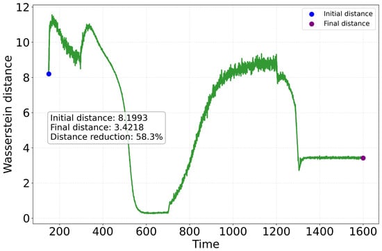
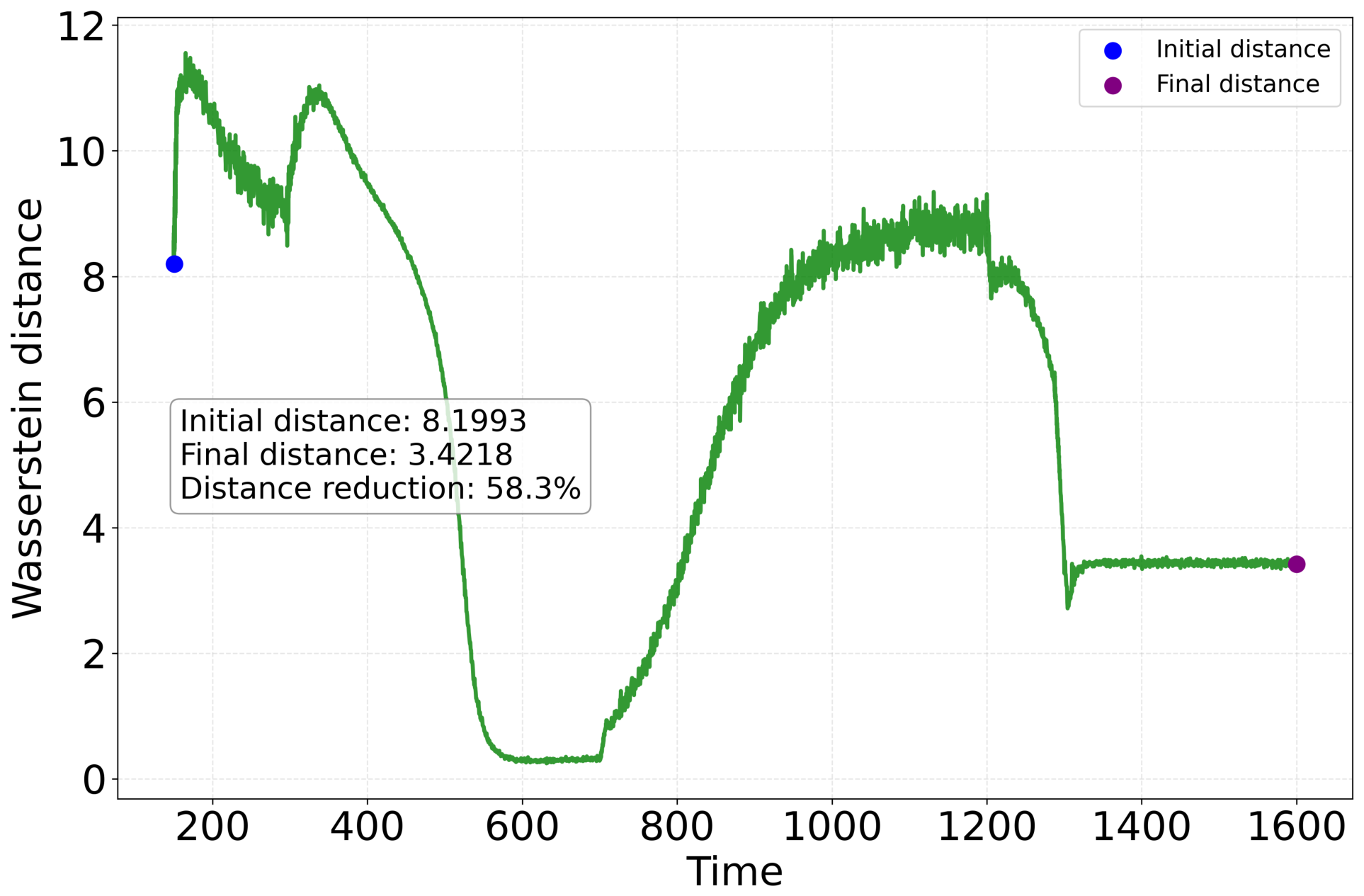
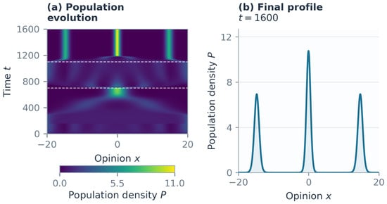
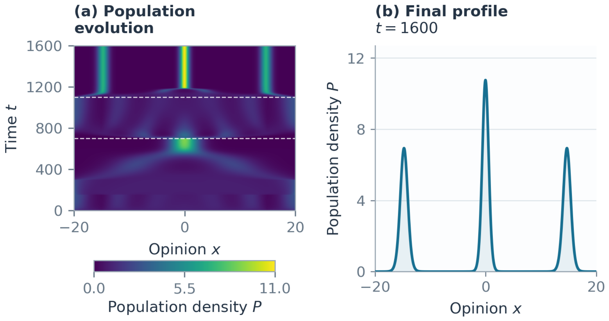

Disclaimer/Publisher’s Note: The statements, opinions and data contained in all publications are solely those of the individual author(s) and contributor(s) and not of MDPI and/or the editor(s). MDPI and/or the editor(s) disclaim responsibility for any injury to people or property resulting from any ideas, methods, instructions or products referred to in the content. |
© 2026 by the authors. Licensee MDPI, Basel, Switzerland. This article is an open access article distributed under the terms and conditions of the Creative Commons Attribution (CC BY) license.