Dynamic Response of Deep V-Shaped Slopes for Incident SH Waves

Abstract

It is essential to explore dynamic response of a deep V-shaped slope for incident SH waves, meeting the challenges of extreme disasters including earthquakes. A novel analytical solution is proposed to effectively evaluate dynamic response of deep V-shaped slopes for incident SH waves. A validation of this solution is confirmed through comparisons with boundary integral equations and another analytical approach. More importantly, it can provide the exact analytical expressions of unknown coefficients of wave functions and present a new idea solving relative problems. The new numerical results show that displacement amplitudes and phases change apparently with the dimensionless distance. Moreover, effects of incident angles, angles of slopes and the dimensionless frequencies to the dynamic response of deep V-shaped slopes are significantly discussed in a wide range of frequencies. Regular patterns of displacement amplitudes are symmetric for vertical incidence. The oscillation numbers of displacement amplitudes on a facing wave surface and its left are often more than these on a shadow surface and its right for oblique and horizontal incidence. However, the regular patterns of displacement phases versus the dimensionless distance are similar. This study would enhance theoretical and practical significance for an analytical approach, wave motion and site effects.

1. Introduction

Extreme disasters including earthquakes pose great threat to human life and developments, so it is quite essential to study dynamic response of elastic wave incidence [1,2]. It makes significant science and engineering sense in some fields, such as in wave motion and earthquake engineering research [3,4]. Moreover, in order to acquire the wave motion principles and site effects of slopes, it is obviously essential to explore dynamic response of a regular deep V-shaped slope for incident SH waves. These would be filled with the theoretical and practical significance.

The dynamic response for incident SH waves has been constantly studied during the past long time, especially focusing on engineering examples and geometry models. For example, Trifunac [5] found transfer function properties of a semi-cylindrical canyon subjected to SH waves through a closed-form solution, and explained site effects of Pacoima canyon. Wong and Trifunac [6] analyzed the scattering patterns of SH waves by a semi-elliptical canyon model through the exact analytical series solution. Sánchez-Sesma and Rosenblueth [7] calculated amplitude response of arbitrary geometry shape canyons for SH waves using boundary integral equations. Cao and Lee [8] presented the scattering and diffraction patterns of SH waves by arbitrary depth-to-width ratio circular cylindrical canyons. Then, Yuan and Liao [9] introduced a new analytical solution to scattering problems of circular-arc canyons of SH wave incidence by infinite equation system truncation and Graf’s addition theorem. Huang and Chiu [10,11] simulated site effects of Feitsui canyon through integral equation methods, concluding the simulated and observed seismograms agree well mostly. Tsaur et al. [12] studied seismic response phenomena of V-shaped canyons in frequency- and time-domains using truncation of infinite equations and an image method. The above studies have enriched the knowledge of the wave motion and site effects for incident SH waves. In recent years, dynamic response studies have been expanding and developing. For example, Song Y et al. [13] investigated seismic response regular patterns of an isosceles triangle hill model subjected to SH waves. Panji M [14] analyzed the surface response of the orthotropic layer using a TD-BEM computation model. Li M et al. [15] discussed wave effects of a coupled semi-cylindrical canyon and hill model for SH waves, according to the elastic wave propagation theory and Fourier transform. In addition, studies also include soil–structure interactions. For instance, Li M et al. [16] and Zhang N et al. [17] separately investigated dynamic interactions of a multi-span bridge with and a simply supported bridge with a V-shaped canyon for incident SH waves. These are also equally caught attention, including amplification effects of slopes under seismic loads [18], dynamic response behavior of a coupled isosceles triangle hill and semi-circular canyon model subjected to SH waves [19], and seismic response of a simplified blocky structure slope model [20].

Despite the knowledge to dynamic response for incident SH waves have been increasing rapidly, it is still needed to study dynamic response of deep V-shaped slopes for incident SH waves. The main computing approaches of dynamic response include analytical and numerical approaches. However, numerical approaches need select computational domain and grid division, may be inefficient for a high frequency, and would be weak or even ineffective in the vicinity of computation model geometric discontinuous points [21,22,23]. Analytical approaches may better avoid above problems of numerical approaches. More importantly, analytical approaches can be used to test numerical approaches and provide a precision guideline for them [21,22,23]. On the other hand, analytical approaches of dynamic response for incident SH waves often need truncate infinite equations with unknown wave functions coefficients [9,12]. Many analytical solutions are also not much concise and efficient. Thus, these would increase the risk of ill-behaved unknown coefficient matrices of equations, consume a number of computational resources, and limit the applicable frequency range of researches. To better avoid the above problems, a novel analytical solution is proposed for evaluating dynamic response of deep V-shaped slopes for incident SH waves. It can provide the exact analytical expressions of unknown coefficients of wave functions, avoiding solving the infinite equation systems. It may therefore address well the practical algorithm theory problem and present a new idea solving relative problems. What is more, in a wide range of frequencies, the influence of factors on the dynamic response of a slope is mainly discussed using the proposed solution, the factors including incident angles, angles of slopes and the dimensionless frequencies.

2. The Methodology

2.1. The Mathematical Model

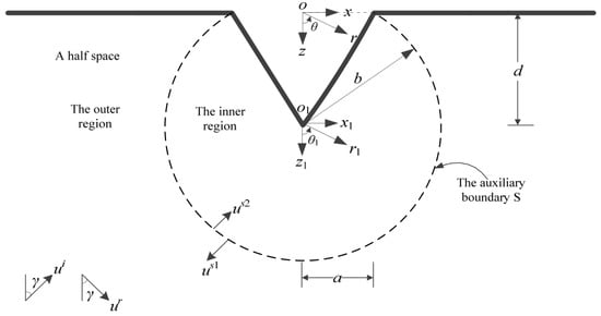
The mathematical model of the deep V-shaped slope is exhibited in Figure 1. It formulates a half space ($z>0$) from which a triangular prism is removed to form the deep V-shaped slope, excited by an SH wave with the displacement amplitude 1, the circular frequency $\omega$ and the incident angle $\gamma$. The incident angle $\gamma$ is measured clockwise from the vertical direction, as shown in Figure 1. The deep V-shaped slope is hypothesized to be isotropic, homogeneous, and linear elastic, possessing the shear wave velocity $c_{\mathrm{s}}$ and the shear modulus $\mu$. It is centered at $O$. It is also characterized by the height $d$ and the half width $a$. The circular-arc auxiliary boundary $\mathrm{S}$ is centered at $O_1$ possessing a radius $b$, dividing the half space into outer region 1 and inner region 2.

Figure 1. The mathematical model of the deep V-shaped slope.

Two Cartesian rectangular coordinate systems are established. One, the $(x,z)$, is centered at $O$. This coordinate system positive $x$ axis points to the right, and its positive $z$ axis points to down. The other, $(x_1,z_1)$, is centered at $O_1$. Its positive $x_1$ axis points to the right, and its positive $z_1$ axis points to down. Two cylindrical coordinate systems, the $(r,\theta )$ with radial distance $r$ and the $(r_1,{\theta }_1)$ with radial distance $r_1$, are also established at $O$ and $O_1$, respectively. The angle $\theta$ is measured counter-clockwise. It is measured from the positive $z$ axis to the positive $x$ axis. The angle ${\theta }_1$ is also measured counter-clockwise. It is measured from the positive $z_1$ axis to the positive $x_1$ axis. Therefore, in the cylindrical coordinate system $(r_1,{\theta }_1)$, the allowable domain of the region 1 is $\left\{\left(r_1,{\theta }_1\right) | {b<r}_1, -(\phi +\pi /2)<{\theta }_1<(\phi +\pi /2)\right\}$. The allowable domain of the region 2 is $\left\{\left(r_1,{\theta }_1\right) | {0\le r}_1\le b, -(\phi +\pi /2)\le {\theta }_1\le (\phi +\pi /2)\right\}$. The definition domain of the circular-arc auxiliary boundary $\mathrm{S}$ is $\left\{\left(r_1,{\theta }_1\right) | r_1=b, -(\phi +\pi /2)\le {\theta }_1\le (\phi +\pi /2)\right\}$.

2.2. The Theory

In the coordinate system $(x,z)$, the incident SH wave displacement $u^i$ is expressed as [24]

$$u^i(x,z,t)=\mathit{exp}\left[-i\omega \left(t-{\displaystyle \frac{x}{c_{\mathrm{x}}}}+{\displaystyle \frac{z}{c_{\mathrm{z}}}}\right)\right]$$

(1)

where $c_{\mathrm{x}}$ and $c_{\mathrm{z}}$ stand for phase velocities along the $x$ and $z$ axis, respectively. Their expressions are able to be given by

$$c_{\mathrm{x}}=c_{\mathrm{s}} /\mathit{sin}\gamma$$

(2)

$$c_{\mathrm{z}}=c_{\mathrm{s}} /\mathit{cos}\gamma$$

(3)

The reflected SH wave displacement $u^r$ illustrated in Figure 1 is written as [24]

$$u^r(x,z,t)=\mathit{exp}\left[-i\omega \left(t-{\displaystyle \frac{x}{c_x}}-{\displaystyle \frac{z}{c_{\mathrm{z}}}}\right)\right]$$

(4)

In the methodology, the time factor $\exp (-i\omega t)$ are omitted. Thus, Equations (1) and (4) become

$$u^i(x,z)=\mathit{exp}\left[-i\omega \left(-{\displaystyle \frac{x}{c_{\mathrm{x}}}}+{\displaystyle \frac{z}{c_{\mathrm{z}}}}\right)\right]$$

(5)

$$u^r(x,z)=\mathit{exp}\left[-i\omega \left(-{\displaystyle \frac{x}{c_{\mathrm{x}}}}-{\displaystyle \frac{z}{c_{\mathrm{z}}}}\right)\right]$$

(6)

In a half space without the deep V-shaped slope, free wavefield displacement $u^{i+r}$ is composed of incident wave displacement $u^i$ and reflected wave displacement $u^r$. It is obtained through the sum of $u^i$ and $u^r$ as follows

$$u^{i+r}=u^i+u^r$$

(7)

The cylindrical coordinate system will be more suitable for problems of the deep V-shaped slope. There employ translation formulae of rectangular coordinate systems to cylindrical coordinate systems

$$x=r_{1}sin{\theta }_1$$

(8)

$$z=r_{1}cos{\theta }_1+d$$

(9)

and Jacobi-Anger expansion formula [25]

$$\mathit{exp}\left(\pm ikrcos\theta \right)=\underset{m=0}{\sum ^{\infty }}{\epsilon }_m{(\pm i)}^m{J}_m\left(kr\right)cos m\theta$$

(10)

This free wavefield displacement in the coordinate system $(r_1,{\theta }_1)$ is expressed as

$$u^{i+r}(r_1,{\theta }_1)=\underset{m=0}{\sum ^{\infty }}{J}_m\left(k{r}_1\right)\left(A_{0,m}\mathit{cos}m{\theta }_1+B_{0,m}\mathit{sin}m{\theta }_1\right)$$

(11)

with

$$\left\{\begin{array}{c}{A}_{0,m}\\ B_{0,m}\end{array}\right\}={\epsilon }_m{i}^m[\pm {\left(-1\right)}^m\mathit{exp}\left(-ikdcos\gamma \right)+\mathit{exp}\left(ikdcos\gamma \right)]\left\{\begin{array}{c}\mathit{cos}m\gamma \\ \mathit{sin}m\gamma \end{array}\right\}$$

(12)

where $J_m\left(x\right)$ are first kind Bessel functions with order $m$ in Equations (10) and (11), with ${\mathsf{\epsilon }}_m=1$ for $m=0$ and ${\epsilon }_m=2$ for $m>0$ in Equations (10)–(12). $k$ represents the circular wave number in a half space as follows

$$k=\omega /c_{\mathrm{s}}$$

(13)

The auxiliary boundary $\mathrm{S}$ is employed to address the problems better. Because of the auxiliary boundary $\mathrm{S}$, there will be a cylindrical outgoing wave $u^{s1}$ in outer region 1 and a cylindrical standing wave $u^{s2}$ in inner region 2 as illustrated in Figure 1. The total wavefield displacement, including the free wavefield, the cylindrical outgoing wave and standing wave displacement, must satisfy the wave motion equation in cylindrical coordinate systems

$${\displaystyle \frac{{\mathsf{\partial }}^{2}u}{\mathsf{\partial }{r}^2}}+{\displaystyle \frac{1}{r}}{\displaystyle \frac{\mathsf{\partial }u}{\mathsf{\partial }r}}+{\displaystyle \frac{1}{r^2}}{\displaystyle \frac{{\mathsf{\partial }}^{2}u}{\mathsf{\partial }{\theta }^2}}={\displaystyle \frac{1}{c^2}}{\displaystyle \frac{{\mathsf{\partial }}^{2}u}{\mathsf{\partial }{t}^2}}$$

(14)

where $c$ represents the shear wave velocity.

Stress-free boundary conditions at half space surface (slope top surface) and slope surface can be written as

$${\tau }_{\theta y}={\displaystyle \frac{\mu }{r}}{\displaystyle \frac{\mathsf{\partial }u}{\mathsf{\partial }\theta }}=0 \mathrm{at} \theta =\pm \pi /2,r>a$$

(15)

$${\tau }_{{\theta }_{1}y}={\displaystyle \frac{\mu }{r_1}}{\displaystyle \frac{\mathsf{\partial }u}{\mathsf{\partial }{\theta }_1}}=0 \mathrm{at} {\theta }_1=\pm (\phi +\pi /2)$$

(16)

where $\phi =\mathrm{a}\mathrm{r}\mathrm{c}\mathrm{t}\mathrm{a}\mathrm{n}(d/a)$ are angles of slopes. $\tau$ represents the shear stress.

The cylindrical outgoing wave consists of scattered and diffracted waves. The cylindrical standing wave consists of transmitted and scattered waves. The cylindrical outgoing wave displacement $u^{s1}$ must satisfy the wave motion Equation (14) without the time factor and the stress-free boundary condition Equation (15). Therefore, it is obtained as follows

$$u^{s1}(r,\theta )=\underset{n=0}{\sum ^{\infty }}\left[H_{2n}^{\left(1\right)}\left(kr\right)A_{1,2n}cos2n\theta +H_{2n+1}^{\left(1\right)}\left(kr\right)B_{1,2n+1}\mathit{sin}\left(2n+1\right)\theta \right]$$

(17)

where $H_n^{\left(1\right)}\left(x\right)$ are first kind Hankel functions with order $n$.

The cylindrical standing wave displacement $u^{s2}$ must satisfy the wave motion Equation (14) without the time factor and the stress-free boundary condition Equation (16). Therefore, it is obtained as follows

$$u^{s2}(r_1,{\theta }_1)=\underset{m=0}{\sum ^{\infty }}\left[J_{2m\upsilon }\left(k{r}_1\right)A_{2,2m\upsilon }cos2m\upsilon {\theta }_1+J_{\left(2m+1\right)\upsilon }\left(k{r}_1\right)B_{2,\left(2m+1\right)\upsilon }\mathit{sin}\left(2m+1\right)\upsilon {\theta }_1\right]$$

(18)

where $\upsilon =\mathsf{\pi }/(2\phi +\mathsf{\pi })$.

In the next study, it is necessary to transform $u^{s1}$ from the cylindrical coordinate system $(r,\theta )$ into the cylindrical coordinate system $(r_1,{\theta }_1)$ through Graf’s addition theorem [8,9,26]. It is given by

$$C_n\left(r\right)\left\{\begin{array}{c}cosn\theta \\ sinn\theta \end{array}\right\}=\underset{m=0}{\sum ^{\infty }}{\displaystyle \frac{{\epsilon }_m}{2}}\left[J_{m-n}\left(d\right)\pm {\left(-1\right)}^n{J}_{m+n}\left(d\right)\right]·C_m\left(r_1\right)\left\{\begin{array}{c}cosm{\theta }_1\\ sinm{\theta }_1\end{array}\right\}$$

(19)

where ${C_n\left(x\right)/C}_m\left(x\right)$ are first kind Bessel or Hankel functions with order $n$ or $m$, with ${\mathsf{\epsilon }}_m=1$ for $m=0$ and ${\epsilon }_m=2$ for $m>0$.

By Equation (19), the cylindrical outgoing wave displacement $u^{s1}$ in the cylindrical coordinate system $(r_1,{\theta }_1)$ is able to be obtained as follows

$$u^{s1}(r_1,{\theta }_1)=\underset{m=0}{\sum ^{\infty }}{H}_m^{\left(1\right)}\left(k{r}_1\right)(A_{1,m}cosm{\theta }_1+B_{1,m}\mathit{sin}m{\theta }_1)$$

(20)

and

$$\left\{\begin{array}{c}{A}_{1,m}\\ B_{1,m}\end{array}\right\}=\underset{n=0}{\sum ^{\infty }}\left\{\begin{array}{c}{\displaystyle \frac{{\epsilon }_n}{2}}\left[J_{2n-m}\left(kd\right)+{\left(-1\right)}^m{J}_{2n+m}\left(kd\right)\right]A_{1,2n}\\ {\displaystyle \frac{{\epsilon }_n}{2}}\left[J_{2n+1-m}\left(kd\right)-{\left(-1\right)}^m{J}_{2n+1+m}\left(kd\right)\right]B_{1,2n+1}\end{array}\right\}$$

(21)

with ${\mathsf{\epsilon }}_n=1$ for $n=0$ and ${\epsilon }_n=2$ for $n>0$.

The auxiliary boundary $\mathrm{S}$ makes a solution of problems more effective. However, it is necessary to eliminate effects of this auxiliary boundary. These continuity boundary conditions at the circular-arc auxiliary boundary $\mathrm{S}$ in the cylindrical coordinate system $(r_1,{\theta }_1)$ can be written as

$$u^1(r_1,{\theta }_1)=u^2(r_1,{\theta }_1) \mathrm{at} r_1=b$$

(22)

$${\tau }_{r_{1}y}^1(r_1,{\theta }_1)=\mu {\displaystyle \frac{\mathsf{\partial }u}{\mathsf{\partial }{r}_1}}={\tau }_{r_{1}y}^2(r_1,{\theta }_1) \mathrm{at} r_1=b$$

(23)

The wavefield $u^1$ in outer region 1 consists of this free wavefield $u^{i+r}$ and this cylindrical outgoing wave $u^{s1}$. The wavefield $u^2$ in inner region 2 consists of the cylindrical standing wave $u^{s2}$. The wavefield $u^1$ and $u^2$ displacement must satisfy the wave motion Equation (14) without the time factor. In addition, the wavefield $u^1$ and $u^2$ displacement also must satisfy these continuity boundary conditions Equations (22) and (23). Substituting $u^{i+r}+u^{s1}$ and $u^{s2}$ into the boundary conditions (22) and (23), and using the determinant techniques, exact analytical expressions of unknown coefficients $A_{1,m}$, $B_{1,m}$, $A_{2,2m\upsilon }$ and $B_{2,\left(2m+1\right)\upsilon }$ are derived as follows

$$A_{1,m}={\displaystyle \frac{\left|\begin{array}{cc}{J}_{2m\upsilon }\left(kb\right)cos2m\upsilon {\theta }_1& A_{0,m}{J}_m\left(kb\right)cosm{\theta }_1\\ J_{2m\upsilon }^{\prime }\left(kb\right)cos2m\upsilon {\theta }_1& A_{0,m}{J}_m^{\prime }\left(kb\right)cosm{\theta }_1\end{array}\right|}{∆1}}$$

(24)

$$B_{1,m}={\displaystyle \frac{\left|\begin{array}{cc}{J}_{\left(2m+1\right)\upsilon }\left(kb\right)\mathit{sin}\left(2m+1\right)\upsilon {\theta }_1& B_{0,m}{J}_m\left(kb\right)sinm{\theta }_1\\ J_{\left(2m+1\right)\upsilon }^{\prime }\left(kb\right)\mathit{sin}\left(2m+1\right)\upsilon {\theta }_1& B_{0,m}{J}_m^{\prime }\left(kb\right)sinm{\theta }_1\end{array}\right|}{∆2}}$$

(25)

$$A_{2,2m\upsilon }={\displaystyle \frac{\left|\begin{array}{cc}{A}_{0,m}{J}_m\left(kb\right)cosm{\theta }_1& -H_m^{\left(1\right)}\left(kb\right)cosm{\theta }_1\\ A_{0,m}{J}_m^{\prime }\left(kb\right)cosm{\theta }_1& {-H}_m^{\prime \left(1\right)}\left(kb\right)cosm{\theta }_1\end{array}\right|}{∆1}}$$

(26)

$$B_{2,\left(2m+1\right)\upsilon }={\displaystyle \frac{\left|\begin{array}{cc}{B}_{0,m}{J}_m\left(kb\right)sinm{\theta }_1& -H_m^{\left(1\right)}\left(kb\right)sinm{\theta }_1\\ B_{0,m}{J}_m^{\prime }\left(kb\right)sinm{\theta }_1& {-H}_m^{\prime \left(1\right)}\left(kb\right)sinm{\theta }_1\end{array}\right|}{∆2}}$$

(27)

with

$$∆1=\left|\begin{array}{cc}{J}_{2m\upsilon }\left(kb\right)cos2m\upsilon {\theta }_1& -H_m^{\left(1\right)}\left(kb\right)cosm{\theta }_1\\ J_{2m\upsilon }^{\prime }\left(kb\right)cos2m\upsilon {\theta }_1& {-H}_m^{\prime \left(1\right)}\left(kb\right)cosm{\theta }_1\end{array}\right|$$

(28)

$$∆2=\left|\begin{array}{cc}{J}_{\left(2m+1\right)\upsilon }\left(kb\right)\mathit{sin}\left(2m+1\right)\upsilon {\theta }_1& -H_m^{\left(1\right)}\left(kb\right)sinm{\theta }_1\\ J_{\left(2m+1\right)\upsilon }^{\prime }\left(kb\right)\mathit{sin}\left(2m+1\right)\upsilon {\theta }_1& {-H}_m^{\prime \left(1\right)}\left(kb\right)sinm{\theta }_1\end{array}\right|$$

(29)

where $J_m^{\prime }\left(x\right)$ represent first kind Bessel derived functions with order $m$, $H_m^{\prime \left(1\right)}\left(x\right)$ first kind Hankel derived functions with order $m$.

3. Numerical Results

Finding amplitudes and phases patterns and interpreting surface motion and site effect are interested in the wave motion and earthquake engineering research. However, the wavefield displacement is the complex number in the methodology. It is necessary to acquire the wavefield displacement amplitudes and phases through

$$\left|u\right|={\left[{(Re u)}^2+{(Im u)}^2\right]}^{1/2}$$

(30)

$$\varphi ={\mathit{tan}}^{-1}\left({\displaystyle \frac{Im u}{Re u}}\right)$$

(31)

In order to reflect true wavefield displacement phases, a phase unwrapping method will be employed in the follow study. There is the principle of this method as follows. When the jumps between consecutive displacement phases $\varphi$ are greater than or equal to $\pi$ radians, these displacement phases $\varphi$ are shifted by adding an integer multiple of $\pm 2\pi$ radians.

The width of the deep V-shaped slope and the wavelength of the SH wave are able to be combined well to enhance interpretations. The dimensionless frequency expression is given by

$$\eta ={\displaystyle \frac{2a}{\lambda }}={\displaystyle \frac{\omega a}{\pi c_{\mathrm{s}}}}$$

(32)

where $\eta$ represents the dimensionless frequency. $\lambda$ are the wavelengths of incident SH waves.

3.1. Parameters of Examples

The surface motion of the deep V-shaped slope is only concerned, since it is more essential for the wave motion and earthquake engineering research. There will be 20 numerical examples in the next study. The factors, including the incident angle $\gamma$, the angle of the slope $\phi$ and the dimensionless frequency $\eta$, are interested in the research. The parameters of numerical examples are exhibited in Table 1.

Table 1. The parameters of numerical examples.

Number	$\mathit{\gamma }/°$	$\mathit{\phi }/°$	$\mathit{\eta }$	$\mathit{x}/\mathit{a}$	Number	$\mathit{\gamma }/°$	$\mathit{\phi }/°$	$\mathit{\eta }$	$\mathit{x}/\mathit{a}$
1	0	45	0.25	$\left[-4,4\right]$	11	30	45	2	$\left[-4,4\right]$
2	0	64	0.2	$\left[-4,4\right]$	12	45	45	2	$\left[-4,4\right]$
3	30	45	5	$\left[-4,4\right]$	13	60	45	2	$\left[-4,4\right]$
4	30	75	5	$\left[-4,4\right]$	14	90	45	1	$\left[-4,4\right]$
5	30	45	10	$\left[-4,4\right]$	15	90	52	1	$\left[-4,4\right]$
6	30	75	10	$\left[-4,4\right]$	16	90	60	1	$\left[-4,4\right]$
7	60	45	0.5	$\left[-4,4\right]$	17	45	45	1:50	0
8	60	60	0.5	$\left[-4,4\right]$	18	45	45	1:50	1
9	60	45	5	$\left[-4,4\right]$	19	45	45	1:50	2
10	60	60	5	$\left[-4,4\right]$	20	45	45	1:50	3

3.2. Analyses of Results

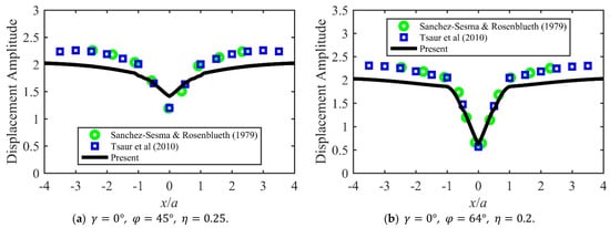
The comparisons with other study results are produced to strongly prove the correctness and availability of this novel analytical solution. The displacement amplitudes of numerical examples 1 and 2 are shown in Figure 2 for the comparisons with results of Sánchez-Sesma & Rosenblueth and of Tsaur et al. Sánchez-Sesma & Rosenblueth used boundary integral equations in their paper, and Tsaur et al. used an analytical approach in their paper. Figure 2a illustrates that displacement amplitudes vary with dimensionless distance $x/a$ for the incident SH wave angle $\gamma =0°$, the angle of the slope $\phi =45°$ and the dimensionless frequency $\eta =0.25$. Figure 2b illustrates that displacement amplitudes vary with dimensionless distance $x/a$ for the incident SH wave angle $\gamma =0°$, the angle of the slope $\phi =64°$ and the dimensionless frequency $\eta =0.2$. The dimensionless distance range plotted is from −4 to 4 in Figure 2.

Figure 2. The comparisons with results of Sánchez-Sesma & Rosenblueth (1979) [7] and of Tsaur et al. (2010) [12].

It can be clearly found that the comparisons between results of the present, and of Sánchez-Sesma & Rosenblueth and Tsaur et al. are consistent. Differences between results of the present and of other two solutions also occur in responses of the half space free surface (slope top surface) since numerical approximation techniques and Bessel function assumptions are differences. For example, Sánchez-Sesma & Rosenblueth employed a first kind Fredholm integral equation and considered the outside boundary integration path. Tsaur et al. employed second kind Hankel functions and considered truncation of infinite equations and an image method. These confirm that the novel analytical solution proposed is effective and applicable for studying the dynamic response of deep V-shaped slopes for incident SH waves.

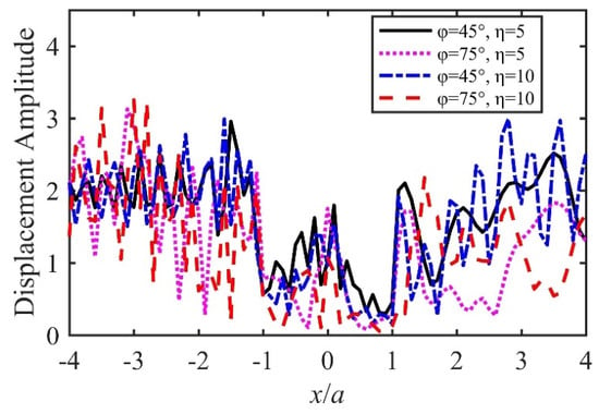
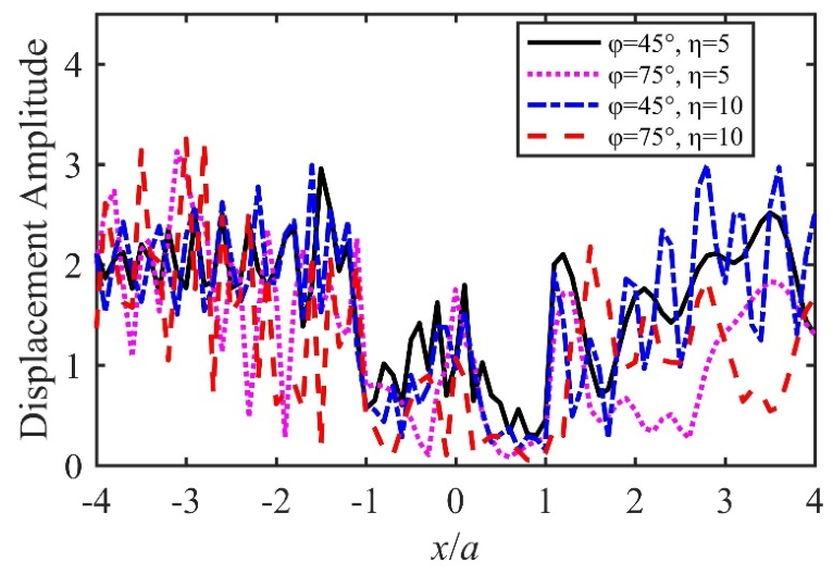
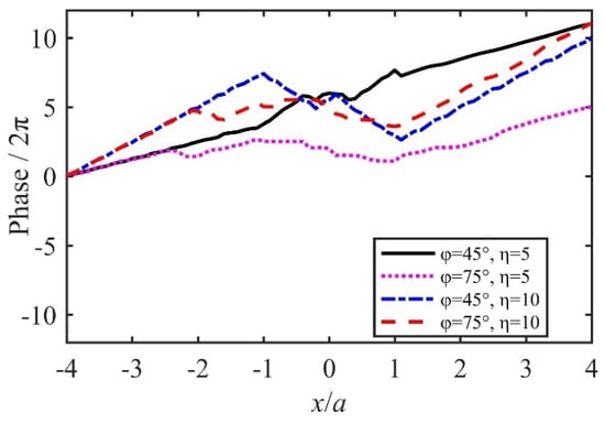
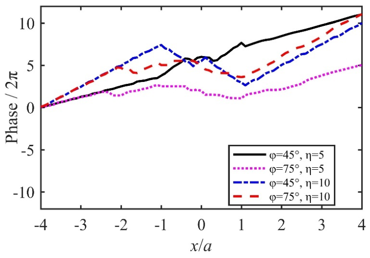
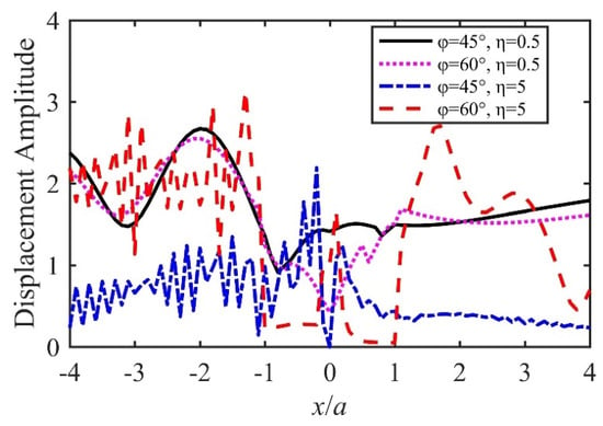
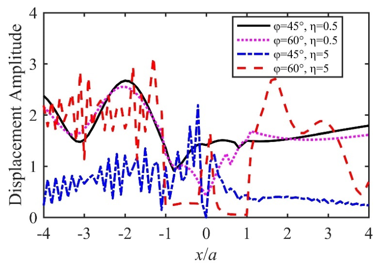
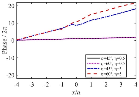
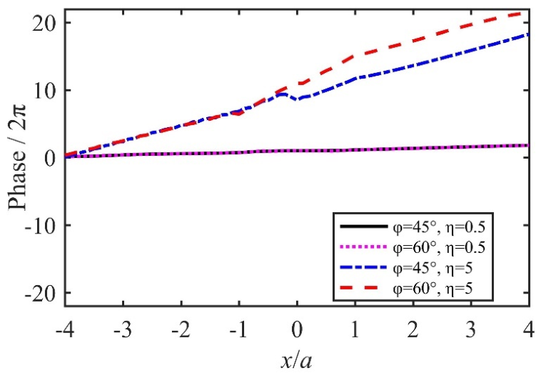
It is necessary to further focus on the interpretation of the results to enhance its impact. The displacement amplitudes and phases of numerical examples 3, 4, 5 and 6 are separately shown in Figure 3 and Figure 4. Figure 3 illustrates the regular patterns of displacement amplitudes versus dimensionless distance for the above four numerical examples. It is obvious to find the displacement amplitudes changes from one point to another for the incident angle $\gamma =30°$. The regular patterns of displacement amplitudes are more complicated as frequencies increase for the angles of the slopes $\phi =45°$ and $75°$. The free wavefield displacement amplitudes would be equal to 2 when considering the amplification value of displacement amplitudes. Thus, it is obvious to discover the largest amplification value of displacement amplitudes is less than 2 for the above four numerical examples. The dimensionless distance of the slope surface is within the range from −1 to 1. Thus, displacement amplitudes on a slope surface are often smaller than these on a half space free surface (slope top surface) for these numerical examples. Figure 4 illustrates the regular patterns of displacement phases versus the dimensionless distance for the above four numerical examples. The phase general trends are similar for the numerical examples. However, the maximum of phases divided by $2\mathsf{\pi }$, the $\varphi /2\mathsf{\pi }$ maximum, does not exceed 10 for $\phi =75°$ and $\eta =5$. In addition, there are no sharp jumps in the variations of displacement phases for the numerical examples.

Figure 3. The displacement amplitudes presented for $\gamma =30°$

Figure 4. The displacement phases presented for $\gamma =30°$

The displacement amplitudes and phases of numerical examples 7, 8, 9 and 10 are separately shown in Figure 5 and Figure 6. Figure 5 illustrates the regular patterns of displacement amplitudes versus dimensionless distance for the above four numerical examples. The variations of these vary evidently from each other for the incident angle $\gamma =60°$. For example, the diagrams for the low frequency $\eta =0.5$ are smoother than these for the high frequency $\eta =5$. It is also obvious to find the largest amplification value of displacement amplitudes is less than two for the above four numerical examples. For the frequency $\eta =0.5$, the displacement amplitudes for the large angle of the slope $\phi =60°$ are often less than these for the small angle of the slope $\phi =45°$ on the slope surface. In addition, for the frequency $\eta =5$, the displacement amplitudes for the large angle of the slope $\phi =60°$ are often less than these for the small angle of the slope $\phi =45°$ on the slope surface. However, for the frequency $\eta =5$, the displacement amplitudes for the large angle of the slope $\phi =60°$ are often more than these for the small angle of the slope $\phi =45°$ on the half space free surface (slope top surface). Figure 6 illustrates the regular patterns of displacement phases versus the dimensionless distance for the above four numerical examples. The phase general trends are nearly same for $\phi =45°$, $\eta =0.5$ and $\phi =60°$, $\eta =0.5$. However, the phase general trends are similar for $\phi =45°$, $\eta =5$ and $\phi =60°$, $\eta =5$. There are also no sharp jumps in the variations of displacement phases for the numerical examples.

Figure 5. The displacement amplitudes presented for $\gamma =60°$

Figure 6. The displacement phases presented for $\gamma =60°$

4. Discussion

It is essential and interesting to explore effects of incident SH wave angles, angles of slopes and the dimensionless frequencies to the dynamic response of deep V-shaped slopes for the wave motion and earthquake engineering research. Therefore, constructive discussion has been included below.

4.1. Effect of Incident Angles

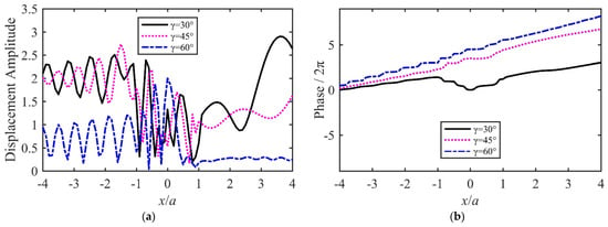
Effect of incident angles means influence of incident SH wave angle changes to the dynamic response under the same conditions. The needed examples are presented in numerical examples 11, 12, and 13 of Table 1 for studying effect of incident angles. The displacement amplitudes and phases of numerical examples 11, 12, and 13 are shown in Figure 7. Figure 7a illustrates the regular patterns of displacement amplitudes versus dimensionless distance for various incident angles in the above three numerical examples. The displacement amplitudes for the incident angles $\gamma =30°$ and $45°$ are more than these for the incident angles $\gamma =60°$ on the half space surface (the slope top surface) for $\phi =45°$, $\eta =2$. As may be observed from Figure 7a, peak displacement amplitudes decrease with increase in incident angles. Figure 7b illustrates the regular patterns of displacement phases versus dimensionless distance for the various incident angles in the above three numerical examples. It is obvious to find displacement phases increase with increase in incident angles from Figure 7b. The phase general trends are similar for $\gamma =45°$ and $60°$. However, the displacement phase curve is similar to a parabola on the slope surface for $\gamma =30°$.

Figure 7. The effect of incident angles for $\phi =45°$, $\eta =2$. (a) The displacement amplitudes presented for incident angles. (b) The displacement phases presented for incident angles.

4.2. Effect of Angles of Slopes

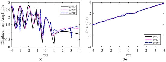
The effect of angles of slopes means the dynamic response changes for various angles of slopes under the same conditions. The needed examples are presented in numerical examples 14, 15, and 16 of Table 1 for studying the effect of angles of slopes. The displacement amplitudes and phases of numerical examples 14, 15, and 16 are shown in Figure 8. Figure 8a illustrates the regular patterns of displacement amplitudes versus dimensionless distance for various angles of slopes in the above three numerical examples. It is obvious that the largest amplification value of displacement amplitudes is less than 1.5 for the above three numerical examples. The dimensionless distance ranges from 0 to 1, corresponding to a shadow surface of a deep V-shaped slope. Thus, the displacement amplitudes for the angle of the slope $\phi =52°$ are more than or equal to these for the angle of the slope $\phi =45°$ on the shadow and right half space surface (slope top surface) for the numerical examples. As may be observed from Figure 8a, peak displacement amplitudes decrease with increase in angles of slopes. Figure 8b illustrates the regular patterns of displacement phases versus dimensionless distance for the various angles of slopes in the above three numerical examples. It is obvious to find the phase general trends are nearly same for the various angles of slopes from Figure 8b. There are no sharp jumps in the variations of displacement phases for the numerical examples.

Figure 8. The effect of angles of slopes for $\gamma =90°$, $\eta =1$. (a) The displacement amplitudes presented for angles of slopes. (b) The displacement phases presented for angles of slopes.

4.3. Effect of the Dimensionless Frequencies

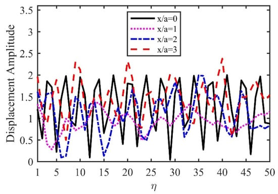
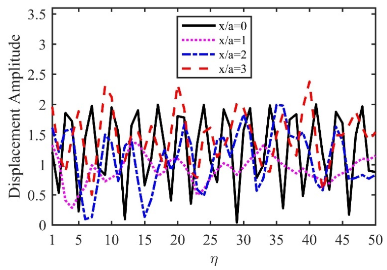
The effect of the dimensionless frequencies is referred to the regular patterns of displacement amplitudes versus the dimensionless frequencies at one point under the same conditions. The displacement amplitudes of numerical examples 17, 18, 19 and 20 are shown in Figure 9. It is obvious to find the largest amplification value of displacement amplitudes is less than 1.5 for the above four numerical examples. The $x/a=0$ corresponds to the slope bottom, $x/a=1$ to the slope right rim (slope shoulder), $x/a=2$ to the point on the right half space free surface (slope top surface) and $x/a=3$ to another point on the right half space free surface (slope top surface). For $\gamma =45°$, $\phi =45°$, and for a dimensionless frequencies range from 1 to 50, the peak displacement amplitude for $x/a=3$ is more than this for the right rim of the slope (slope shoulder) and the peak displacement amplitude for $x/a=2$ is approximately equal to this for the bottom of the slope. Moreover, it is can be clearly found that displacement amplitudes oscillate apparently with increase in dimensionless frequencies at the above four points for $\gamma =45°$, $\phi =45°$.

Figure 9. The effect of the dimensionless frequencies for $\gamma =45°$, $\phi =45°$.

5. Conclusions

A novel analytical solution is proposed to effectively evaluate dynamic response of deep V-shaped slopes for incident SH waves. The presented mathematical model is suitable for slope dynamic research. Angles of slopes range from $45°$ to $75°$ in this study. A validation of this novel analytical solution is confirmed through the comparisons between results of the present and of Sánchez-Sesma & Rosenblueth and Tsaur et al. Although differences between results of the present and of other two solutions occur in responses of the half space free surface (slope top surface), displacement amplitude maximum absolute difference is only approximately 0.2. These are reasonable in the practical theory research and engineering application.

Comparison to Tsaur et al.’s approach, the step number of this solution is smaller; the condition number of the coefficient matrices is also smaller. The proposed solution is filled with physical interpretability and consistency. More importantly, it can exactly provide the analytical expressions of unknown coefficients of wave functions, avoiding solving the infinite equation systems and presenting a new idea solving relative problems. In addition, it is also effective and applicable for practical complex cases and a wide range of frequencies, since the mathematical model and auxiliary boundary are flexible and the algorithm theory is advanced and strong.

The 20 numerical examples are applied in the study. It is obvious to discover the largest amplification value of displacement amplitudes is less than 2 for the 20 numerical examples. This amplification character nearly aligns with many actual study and practical case amplification character. This amplification character also nearly aligns with some field or centrifuge/shaking-table observations. For vertical incidence, the regular patterns of displacement amplitudes versus dimensionless distance are symmetric, since this incident angle is $\gamma =0°$ and the mathematical model is symmetric.

The displacement amplitudes on a shadow surface and its right are often smaller than these on a facing wave surface and its left for oblique incidence. The oscillation numbers of displacement amplitudes on a facing wave surface and its left are often more than these on a shadow surface and its right. However, the regular patterns of displacement phases versus the dimensionless distance are similar. The phenomena for horizontal incidence are almost similar to these for oblique incidence. These new findings imply a primary engineering application indication. Significant engineering structures, such as rail transport systems, important houses and cable car systems, could be built safer on the shadow surfaces of and their right of deep V-shaped slopes.

The effects of incident angles, angles of slopes and the dimensionless frequencies are studied in detail, because these are vital for wave motion and earthquake engineering research. The peak displacement amplitudes decrease with increase in incident angles for $\phi =45°$, $\eta =2$. The phase general trends are nearly same for the various angles of slopes for $\gamma =90°$, $\eta =1$. The displacement amplitudes oscillate apparently with increase in dimensionless frequencies at the points from Figure 9 for $\gamma =45°$, $\phi =45°$. These findings provide the new knowledge regarding the wave motion and site effects of deep V-shaped slopes for incident SH waves. These new findings also provide quantitative references and scientific and technological guidance for geotechnical and underground engineering construction and protection. However, the application of the novel analytical solution proposed may be further enhanced, and more practical dynamic response problems of V-shaped slopes should be studied in the future.

References

- Kusiak, A. Extreme Science and Engineering. J. Intell. Manuf. 2020, 31, 1607–1610. [Google Scholar] [CrossRef] [Scilit] [PubMed]
- Abdrakhmatov, K.; Arrowsmith, R.; Elliott, J.; Grutzner, C.; Mukambayev, A.; Rizza, M.; Shnizai, Z.; Walker, R.; Weldon, R.; Wilkinson, R. Urgent Need for Greater Earthquake Resilience in Continental Asia. Nat. Geosci. 2024, 17, 818–819. [Google Scholar] [CrossRef] [Scilit]
- Chang, H.; Wang, F.; Yue, X.; Qiu, L.; Sun, L. A 2.5D Generalized Finite Difference Method for Elastic Wave Propagation Problems. Mathematics 2025, 13, 1249. [Google Scholar] [CrossRef] [Scilit]
- Hossain, A.S.M.F.; Saeidi, A.; Salsabili, M.; Nastev, M.; Suescun, J.R.; Bayati, Z. A Review of Parameters and Methods for Seismic Site Response. Geosciences 2025, 15, 128. [Google Scholar] [CrossRef] [Scilit]
- Trifunac, M.D. Scattering of Plane Sh Waves by a Semi-cylindrical Canyon. Earthq. Eng. Struct. Dyn. 1973, 1, 267–281. [Google Scholar] [CrossRef] [Scilit]
- Wong, H.L.; Trifunac, M.D. Scattering of Plane Sh Waves by a Semi-elliptical Canyon. Earthq. Eng. Struct. Dyn. 1974, 3, 157–169. [Google Scholar] [CrossRef] [Scilit]
- Sánchez-Sesma, F.J.; Rosenblueth, E. Ground Motion at Canyons of Arbitrary Shape under Incident Sh Waves. Earthq. Eng. Struct. Dyn. 1979, 7, 441–450. [Google Scholar] [CrossRef] [Scilit]
- Cao, H.; Lee, V.W. Scattering of Plane SH Waves by Circular Cylindrical Canyons with Variable Depth-to-Width Ratio. Eur. J. Earthq. Eng. 1989, III, 29–37. [Google Scholar]
- Yuan, X.; Liao, Z.P. Scattering of Plane SH Waves by a Cylindrical Canyon of Circular-Arc Cross-Section. Soil Dyn. Earthq. Eng. 1994, 13, 407–412. [Google Scholar] [CrossRef] [Scilit]
- Huang, H.-C.; Chiu, H.-C. The Effect of Canyon Topography on Strong Ground Motion at Feitsui Damsite: Quantitative Results. Earthq. Eng. Struct. Dyn. 1995, 24, 977–990. [Google Scholar] [CrossRef] [Scilit]
- Huang, H.-C.; Chiu, H.-C. Canyon Topography Effects on Ground Motion at Feitsui Damsite. Soil Dyn. Earthq. Eng. 1999, 18, 87–99. [Google Scholar] [CrossRef] [Scilit]
- Tsaur, D.H.; Chang, K.H.; Hsu, M.S. An Analytical Approach for the Scattering of SH Waves by a Symmetrical V-Shaped Canyon: Deep Case. Geophys. J. Int. 2010, 183, 1501–1511. [Google Scholar] [CrossRef] [Scilit]
- Song, Y.; Li, X.; Yang, Z.; Yang, Y.; Sun, M. Seismic Response for an Isosceles Triangle Hill Subjected to Anti-Plane Shear Waves. Acta Geotech. 2022, 17, 275–288. [Google Scholar] [CrossRef] [Scilit]
- Panji, M. A Half-Space TD-BEM Model for a Seismic Corrugated Orthotropic Stratum. Eng. Anal. Bound. Elem. 2023, 152, 655–677. [Google Scholar] [CrossRef] [Scilit]
- Li, M.; Yang, Z.; Yang, Y. Wave Effect of Front Topography Based on Modified Time–Frequency Transform Method. Acta Mech. 2023, 234, 3081–3089. [Google Scholar] [CrossRef] [Scilit]
- Li, M.; Yang, Z.; Sun, M.; Yang, Y. Influence of Canyon Topography Amplification Effect and Shielding Effect on Bridge Seismic Response. Arch. Appl. Mech. 2023, 93, 3327–3340. [Google Scholar] [CrossRef] [Scilit]
- Zhang, N.; Wang, L.; Zhang, Y.; Lu, H.; Dai, D.; Cai, G.; Gao, Y. Effect of a V-Shaped Canyon on the Seismic Response of a Bridge under Oblique Incident SH Waves. Earthq. Eng. Struct. Dyn. 2024, 53, 496–514. [Google Scholar] [CrossRef] [Scilit]
- Cheng, H.; Deng, P. An Analytical Investigation of the Topographic Amplification Effects of Slopes under Seismic Loads. Int. J. Geomech. 2024, 24, 04023302. [Google Scholar] [CrossRef] [Scilit]
- An, X.; Song, Y.; Yang, Z.; Zhang, Z. Response of an Isosceles Trapezoidal Hill with a Semicircular Canyon to Plane SH Waves. Waves Random Complex Media 2025, 35, 8494–8512. [Google Scholar] [CrossRef] [Scilit]
- Du, W.; Fu, X.; Sheng, Q.; Chen, J.; Zhou, Y.; Zheng, S. Dynamic Response of Slopes under Near-Field Seismic Excitation Using the Material Point Method. Comput. Geotech. 2025, 180, 107100. [Google Scholar] [CrossRef] [Scilit]
- Yao, Y.; Liu, T.; Zhang, J. A New Series Solution Method for Two-Dimensional Elastic Wave Scattering along a Canyon in Half-Space. Soil Dyn. Earthq. Eng. 2016, 89, 128–135. [Google Scholar] [CrossRef] [Scilit]
- Lin, G.; Li, Z.-Y.; Li, J.-B. A Substructure Replacement Technique for the Numerical Solution of Wave Scattering Problem. Soil Dyn. Earthq. Eng. 2018, 111, 87–97. [Google Scholar] [CrossRef] [Scilit]
- Ren, P.; Chen, S.; Zhang, Y. Analytical Solution to Transient Response of Arc-Shaped Basin Incident by SH Wave. Technol. Earthq. Disaster Prev. 2021, 16, 352–361. (In Chinese) [Google Scholar] [CrossRef]
- Achenbach, J.D. Wave Propagation in Elastic Solids; Elsevier Science Publishers B.V.: Amsterdam, The Netherlands, 1975. [Google Scholar]
- Abramowitz, M.; Stegun, I.A. Handbook of Mathematical Functions, with Formulas, Graphs, and Mathematical Tables; Dover Publications: New York, NY, USA, 1972. [Google Scholar]
- Watson, G.N. A Treatise on the Theory of Bessel Functions, 2nd ed.; Cambridge University Press: Cambridge, UK, 1966. [Google Scholar]
Disclaimer/Publisher’s Note: The statements, opinions and data contained in all publications are solely those of the individual author(s) and contributor(s) and not of MDPI and/or the editor(s). MDPI and/or the editor(s) disclaim responsibility for any injury to people or property resulting from any ideas, methods, instructions or products referred to in the content. |
© 2026 by the authors. Licensee MDPI, Basel, Switzerland. This article is an open access article distributed under the terms and conditions of the Creative Commons Attribution (CC BY) license.