Auxiliary Solutions via Dimension Reduction for the (2+1)-Dimensional Calogero–Bogoyavlenskii–Schiff Equation Based on a Bilinear Neural Network Method Coupled with Symbolic Computation

Abstract

Nonlinear partial differential equations formed the mathematical core of nonlinear science. They revealed the intrinsic link between algebraic structures and complex dynamical behaviors. Traditional analytical and numerical methods, however, faced high computational costs, cumbersome derivations, limited accuracy, and poor generality. They especially struggled to solve high-dimensional integrable systems efficiently. To meet these challenges, this study built on traditional neural network methods. We introduced the Hirota bilinear transformation to convert the original nonlinear equation into a bilinear form. We then constructed a bilinear neural network solving procedure deeply coupled with symbolic computation. This strategy effectively suppressed error accumulation caused by random initialization and approximate approximation in traditional numerical iterative methods. Within this framework, this study constructed complete single-hidden-layer and double-hidden-layer neural network models to obtain analytical solutions of the auxiliary equation. By designing network structures with multiple activation functions, we built diverse trial solutions. We also systematically established a coupling adaptation mechanism among activation functions, network depth, and the bilinear transformation. To verify the effectiveness and robustness of the proposed method, we applied it to the Calogero–Bogoyavlenskii–Schiff (CBS) equation. We successfully derived multiple new exact solutions. We further constructed various neural network models and heuristic strategies. This study provided new ideas for neural network solving of integrable systems. It also offered a feasible path for approximation-free exact solutions of high-dimensional nonlinear partial differential equations. The findings held important theoretical value and broad application prospects in fluid dynamics, optical communication, plasma physics, and related engineering fields.

1. Introduction

Nonlinear partial differential equations (NPDEs) served as the mathematical cornerstone of nonlinear science, applied mathematics, and engineering physics. They drew widespread attention because of their interdisciplinary applications across biological sciences, fluid dynamics, optics, and other fields. Related interdisciplinary findings frequently appeared in the literature [1,2]. These equations established a deep connection between algebraic structures and dynamical behaviors. They served as indispensable analytical tools for interpreting nonlinear evolution phenomena. They accurately depicted the evolutionary nature of various complex systems. These encompassed shallow water waves and multilayer fluid interface wave propagation in fluid dynamics. They also covered ion acoustic waves and magnetohydrodynamic fluctuations in plasma physics. Other examples included optical pulse transmission and planar optical waveguiding in nonlinear optics. High-dimensional integrable nonlinear systems generally governed these scenarios. To deeply explore their evolution laws, scholars successively constructed a series of models. These included the Schrödinger equation, Navier-Stokes (N-S) equation, Boussinesq equation [3], Korteweg-de Vries (KdV) equation, and KP equation. They conducted systematic research in their respective fields [4,5,6].

Once a model is established, solving the problem becomes the central challenge. Due to the inherent complexity of nonlinearity, it is difficult to obtain closed-form solutions for a large number of equations using simple analytical methods. However, with the continuous development of mathematical physics theory, scholars both domestically and internationally have gradually established three mature methodological frameworks: exact solution methods, approximate analytical methods, and high-dimensional non-traveling-wave methods, which have powerfully advanced the development and refinement of the theory for solving nonlinear partial differential equations. In terms of exact solutions, methods such as the inverse scattering transform and the extended tanh expansion have been widely applied to integrable systems such as the KdV equation and the nonlinear Schrödinger equation [7]. These methods can effectively construct analytical solutions for solitons, traveling waves, and periodic waves, and reveal the typical structures and evolutionary characteristics of nonlinear waves. Of course, exact solutions cannot be obtained for all equations; for such complex nonlinear models, approximate analytical methods—such as the Adomian decomposition [8], variational iteration [9], and homotopy perturbation [10]—provide efficient solution pathways. These methods do not rely on small-parameter assumptions and can yield high-precision approximate analytical solutions through iterative approximation, making them more widely applicable. However, as research expands into high-dimensional, variable-coefficient nonlinear evolution equations, traditional traveling-wave methods are gradually revealing their limitations. Methods such as the extended co-residence test and the extended three-wave method, based on the theory of generalized separation of variables, can effectively solve various non-traveling-wave analytical solutions [11,12]. Among these, the extended co-residence test has been successfully applied to the CBS equation studied in this paper [13], enriching the solution space of nonlinear equations and refining the theoretical framework for solving high-dimensional nonlinear systems.

As theories in mathematical physics continue to evolve, traditional analytical and numerical methods have gradually revealed shortcomings such as large data volumes, slow computation speeds, and difficulties in solving high-dimensional problems; computer technology is playing an increasingly critical role in solving nonlinear partial differential equations. M. Raissi et al. pioneered the concept of Physics-Informed Neural Networks (PINNs), which embed physical rules into nonlinear partial differential equations [14,15]. Compared to traditional numerical methods, PINNs embedded partial differential equations into the loss function of neural networks. They removed the reliance on complex structured grids. They used physical equations as constraints to flexibly handle irregular geometric domains. This provided a highly promising general framework for high-dimensional, nonlinear, and inverse problem solving.

Although PINNs had broad prospects, they still faced challenges such as high model complexity and large computational costs. Their solution accuracy was typically measured by numerical error. It was also affected by network structures, training strategies, and optimization processes. These issues have become key bottlenecks limiting their application, and researchers continue to explore more efficient and accurate improvement strategies. To address the issue of lagging computational efficiency, the academic community has introduced adaptive configuration points and multiscale training strategies [16,17], enabling the network to focus on key regions where the physical field undergoes drastic changes; Jnini et al. employed a Gauss–Newton natural gradient optimization method, which increased the convergence rate by several hundred times compared to traditional gradient descent, while combining Green’s functions with numerical differentiation to avoid computational redundancy caused by higher-order automatic differentiation [18]. In terms of accuracy improvement, Karniadakis et al. integrated Gauss–Newton optimization and multi-stage residual correction into the network, pushing the solution accuracy to the machine double-precision limit and applying it to the exploration of singularities in the fluid equations [19]; this work aligns with the overall development trend of physics-informed machine learning [20]; The S-PINN and gPINN proposed by Wu et al. significantly mitigated training instability by strengthening conservation constraints and gradient information [21]. As research continues to advance, PINNs are being continuously refined and expanded. Zhang R.F. et al. also proposed a pioneering solution strategy, namely the bilinear neural network method [22,23,24,25,26], which was subsequently extended to the solution of fractional-order equations [27,28,29]. The basic approach is as follows: First, convert the bilinearizable nonlinear partial differential equation into the Hirota bilinear form. Then, a neural network is constructed to generate auxiliary test functions. After substituting these into the bilinear equation, a system of algebraic equations is established through coefficient matching; the network parameters are solved using Maple; and, finally, the exact analytical solution of the original equation is obtained via an inverse transformation. It should be noted that PINNs and the method in this paper belonged to different paradigms: PINNs aimed to achieve numerical approximation, with accuracy affected by discretization, optimization, and network capacity. In contrast, bilinear neural network methods aimed to construct exact analytical solutions via symbolic computation. Their approach was as follows: convert the bilinearizable equation into the Hirota bilinear form. Construct neural network trial functions. Establish algebraic equations through coefficient matching. Solve parameters with Maple. Obtain the original equation solution through inverse transformation. The obtained solution was verified by a residual identically equal to zero, with zero error in the symbolic sense. Therefore, this paper did not directly benchmark efficiency or accuracy against PINNs. Instead, it provided a complementary exact analytical solving path to PINNs.

Nonlinear wave dynamics had broad applications in fluid mechanics, optical fiber communications, and micro/nano systems. The CBS equation, as an important model in this field, was rooted in fluid dynamics and plasma physics. It mainly characterized the propagation mechanisms of nonlinear waves such as shallow water waves and magnetohydrodynamic disturbances [30,31,32]. In recent years, research on the solution structures and mathematical properties of the CBS equation has attracted widespread attention [33]. In particular, Akram et al. [34] explored inelastic lump-breather interactions and periodic wave dynamics of the generalized CBS equation based on a bilinear neural network architecture. Talib et al. [35] analyzed nonlinear wave interactions and stability in the CBS-nCBS model using the bilinear neural network method. Against this background, this paper aimed to further expand the adaptability and solving capability of the bilinear neural network method on such models.

This paper investigated the following (2+1)-dimensional CBS equation:

$$u_{xt}+a{u}_x{u}_{xy}+b{u}_{xx}{u}_y+u_{xxxy}=0$$

(1)

Here, a and b are real parameters. Bogoyavlenskii and Schiff constructed the CBS equation in different ways. Han et al. [36] adopted generalized bilinear operators and polynomial methods. They systematically studied rational solutions of the generalized CBS equation. This provided an effective path for the bilinearization and exact solution construction of CBS-type equations.

Therefore, this paper focuses on the case of Equation (1) when $a=3,b=3$:

$$u_{xt}+3u_x{u}_{xy}+3u_{xx}{u}_y+u_{xxxy}=0$$

(2)

This paper aimed to apply the bilinear neural network coupled with symbolic computation method (BNNM) to this parameter case. We tested the method’s ability to construct analytical solutions of the bilinear auxiliary equation under different parameter conditions. It should be particularly noted that for the specific parameter branch obtained from the neural network trial functions in this paper, symbolic constraints eliminated the explicit dependence of the auxiliary function f on the spatial variable x. This yielded a dimension-reduced auxiliary solution (that is, it forced the relevant x-direction weight to zero, and the term containing x did not contain t). The whole system still acted jointly through y and t. After the Hirota inverse transformation, this auxiliary function corresponded to the trivial solution $u=0$ of the original CBS equation. Therefore, this work focused on revealing the algebraic structure characteristics of the auxiliary function f. The related images only served to intuitively display its spatial structure. They should not be interpreted as the physical wave field of the original CBS equation. They also did not involve discussions of physical dynamical behaviors such as non-trivial soliton families or elastic collisions.

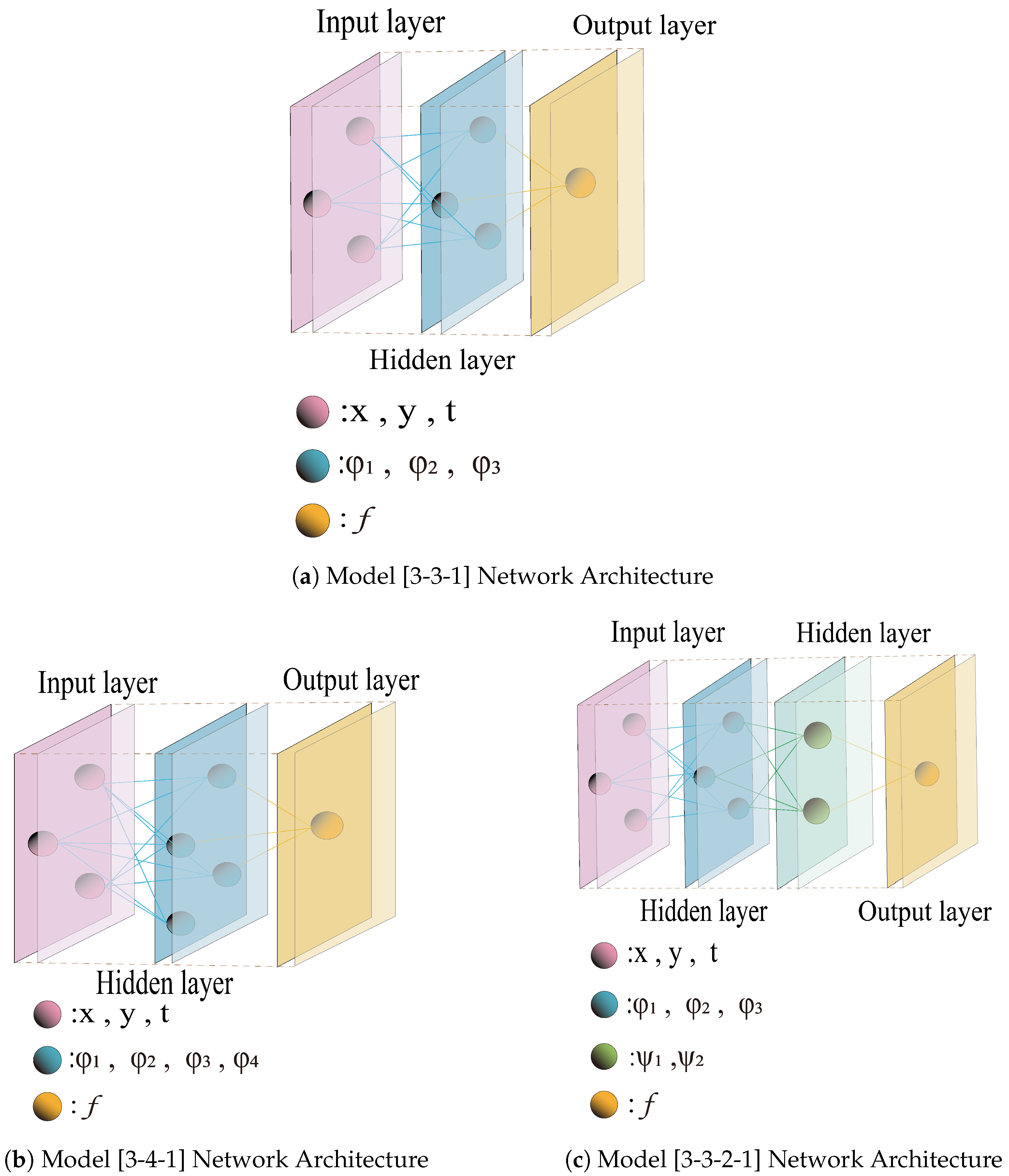
Although the bilinear neural network paradigm was successfully applied to the YTSF equation, Hirota bilinear equation, and Boussinesq equation, this paper focused on applying this framework to the 2+1-dimensional CBS equation containing general parameters a and b. The core work was: within the established bilinear neural network framework, combining neural networks with symbolic computation. We adopted specific network architectures and activation function combinations. We systematically explored the diversity of algebraic structures of the bilinear auxiliary equation. In terms of single-hidden-layer architectures, this paper built a [3-4-1] architecture on the basis of the [3-3-1] model. By increasing the number of hidden layer neurons, we expanded the network’s parameter dimension and mapping capacity at the depth level. This enhanced the ability to capture complex nonlinear algebraic constraints. In terms of double-hidden-layer architectures, we constructed a [3-3-2-1] double-hidden-layer network. Compared with the single-hidden-layer structure, this architecture added more layers at the width level. It achieved multi-level nonlinear mapping and effectively broadened the expression dimension of trial functions. Furthermore, in terms of the activation function system, this paper introduced the Weierstrass P elliptic function into the double-hidden-layer network. This function possessed double periodicity and second-order pole characteristics. Compared with elementary function activation functions in conventional categories, the introduction of the elliptic function enabled trial functions to contain more complex singular manifolds and periodic characteristics. Its coupling with the exponential function successfully constructed a more diverse mixed structure of auxiliary functions. This strategy broke through the limitations of traditional elementary function families. It effectively expanded the algebraic structure boundary of auxiliary equations at the function family level. It provided a function construction space with greater depth and breadth for bilinear neural networks to handle complex integrable systems.

2. Bilinear Neural Network-Coupled Symbolic Computation Method (BNNCSCM)

To transform the (2+1)-dimensional CBS (Calogero–Bogoyavlenskii–Schiff) equations into the Hirota bilinear form suitable for solution by a bilinear neural network, we introduce the Hirota bilinear transformation to convert the original nonlinear equations into a bilinear form.

This paper focuses on the case where a = 3 and b = 3, that is, Equation (2).

Let $f=f(x,y,t)$ be an auxiliary function, and introduce the Hirota transformation:

$$u=2{(lnf)}_x=2{\displaystyle \frac{f_x}{f}}$$

(3)

substituting transformation (3) into Equation (2) and rearranging yields the following bilinear expansion:

$$(D_x{D}_t+D_x^3{D}_y)f·f=0$$

(4)

The Hirota bilinear differential operator is defined as follows:

$$D_x^m{D}_y^n{D}_t^l(f·g)={\left.{({\partial }_x-{\partial }_{x^{\prime }})}^m{({\partial }_y-{\partial }_{y^{\prime }})}^n{({\partial }_t-{\partial }_{t^{\prime }})}^{l}f(x,y,t)g(x^{\prime },y^{\prime },t^{\prime })\right|}_{x^{\prime }=x,y^{\prime }=y,t^{\prime }=t}$$

(5)

Based on the above definition, expanding the bilinear operator in Equation (2) yields the following form of the partial derivatives of the auxiliary function:

$$(D_x{D}_t+D_x^3{D}_y)f·f=2(f_{xt}f-f_t{f}_x)+2f{f}_{xxxy}-6f_x{f}_{xxy}+6f_{xx}{f}_{xy}-2f_{xxx}{f}_y=0$$

(6)

Consequently, the original CBS nonlinear partial differential equation is transformed into a bilinear equation in terms of the auxiliary function f. This form avoids the need to directly handle the complex nonlinear terms of the original equation and provides a foundation for subsequently constructing bilinear neural network exploratory functions and solving for network parameters using symbolic computation methods.

Compared to traditional solution methods, the bilinear neural network method exhibits fundamental differences: traditional PINNs can only obtain numerical approximate solutions, whose accuracy is constrained by various factors such as network structure, training strategies, and loss function design; in contrast, the bilinear neural network method, by constructing a specific bilinear network architecture, can guarantee the accuracy of the solution and directly generate exact analytical solutions that strictly satisfy the original control equation. Furthermore, by integrating symbolic computation, this method effectively overcomes the limitations of traditional numerical methods, such as high computational complexity and significant resource consumption. This paper constructs the following bilinear neural network model:

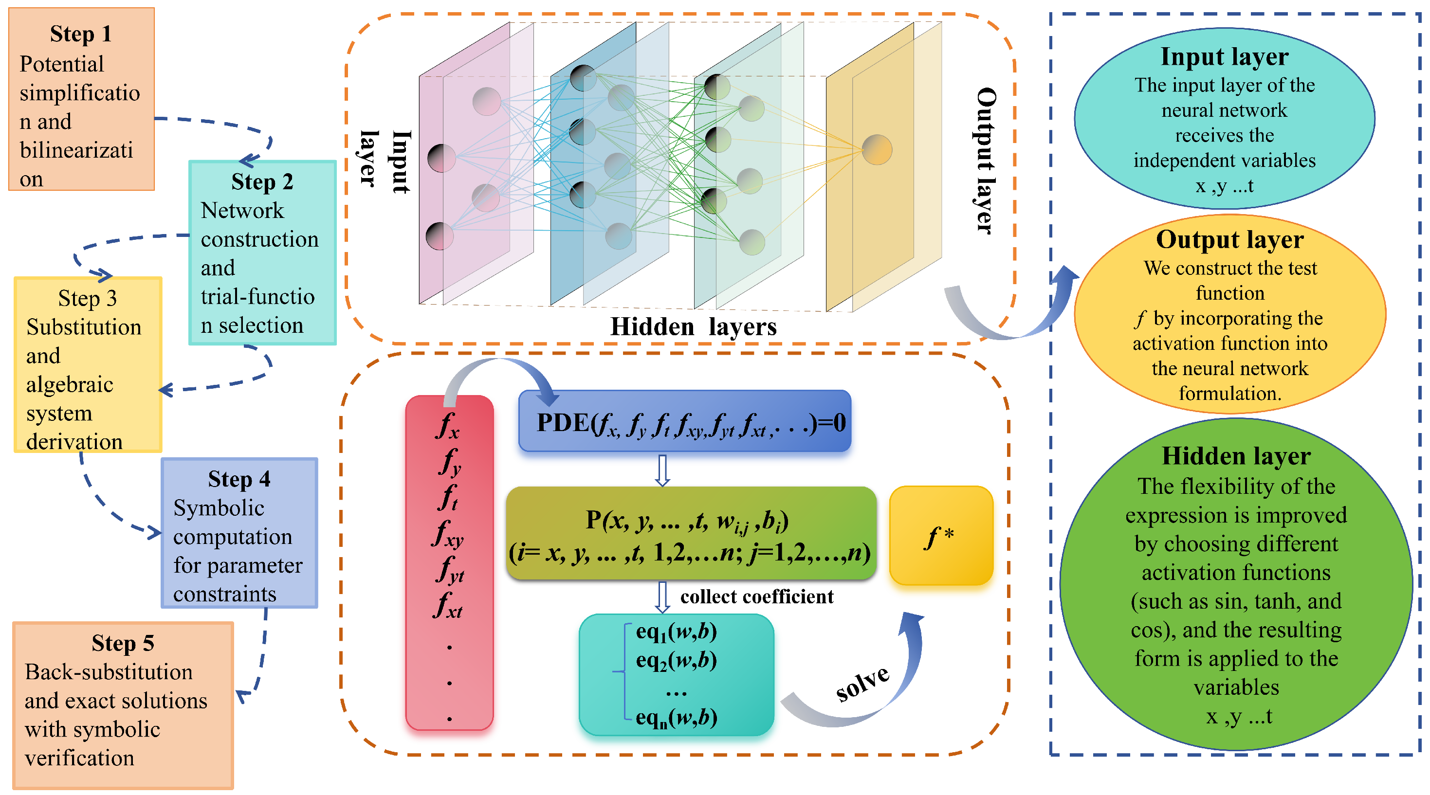
Step 1. Using the Hirota bilinear transformation, we transform the original nonlinear equations into a bilinear form.

Step 2. Based on the neural network model constructed above, we can develop various activation functions for both single-hidden-layer and multi-hidden-layer networks. By experimenting with different activation functions and iteratively replacing the search function, we can identify the optimal search function. The analytical expressions for these networks are as follows:

1.

Single-hidden-layer bilinear neural network

Model [3-3-1]

$$\begin{array}{cc}\hfill f=& w_{1,u}\Phi \left({\xi }_1\right)+w_{2,u}\Phi \left({\xi }_2\right)+w_{3,u}\Phi \left({\xi }_3\right)+b_4\hfill \\ \hfill & {\xi }_i=x{w}_{x,i}+y{w}_{y,i}+t{w}_{t,i}+b_i(i=1,2,3)\hfill \end{array}$$

(7)

Model [3-4-1]

$$\begin{array}{cc}\hfill f=& w_{1,u}\Phi \left({\xi }_1\right)+w_{2,u}\Phi \left({\xi }_2\right)+w_{3,u}\Phi \left({\xi }_3\right)+w_{4,u}\Phi \left({\xi }_4\right)+b_5\hfill \\ \hfill & {\xi }_i=x{w}_{x,i}+y{w}_{y,i}+t{w}_{t,i}+b_i(i=1,2,3,4)\hfill \end{array}$$

(8)

2.

Double-hidden-layer bilinear neural network Model [3-3-2-1]

$$\begin{array}{cc}\hfill & f=w_{4,u}\Phi \left({\xi }_4\right)+w_{5,u}\Phi \left({\xi }_5\right)+b_6\hfill \\ \hfill & {\xi }_i=w_{1,u}\Phi \left({\xi }_1\right)+w_{2,u}\Phi \left({\xi }_2\right)+w_{3,u}\Phi \left({\xi }_3\right)+b_i(i=4,5)\hfill \\ \hfill & {\xi }_i=x{w}_{x,i}+y{w}_{y,i}+t{w}_{t,i}+b_i(i=1,2,3)\hfill \end{array}$$

(9)

Step 3. Substitute the obtained test function expression into the nonlinear micro-differential equation after bilinear transformation, and combine like terms to obtain a system of algebraic equations.

Step 4. Use Maple to perform symbolic computation to solve the system of algebraic equations, obtaining an analytical solution constrained only by weights and thresholds

Step 5. We substituted the parameter constraints into the trial function and obtained the trial solution. We then verified it symbolically in the original CBS Equation (1). For the specific parameter branch from the neural network trial function, symbolic constraints removed the explicit x-dependence of f (the x-direction weight was forced to zero). This yielded a dimension-reduced auxiliary solution. If the residual vanished identically, we identified it as the corresponding dimension-reduced auxiliary analytical solution.

Step 6. For the parameter branch in Section 3.2 that retained the x-direction weight, we substituted the x-containing auxiliary function f into $u=2{\left(lnf\right)}_x$. This yielded an explicit solution u containing x. Symbolic verification in the original CBS equation gave an identically zero residual. Thus, we obtained an x-containing analytical structure complementary to the dimension-reduced auxiliary solution.

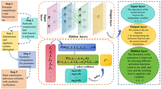
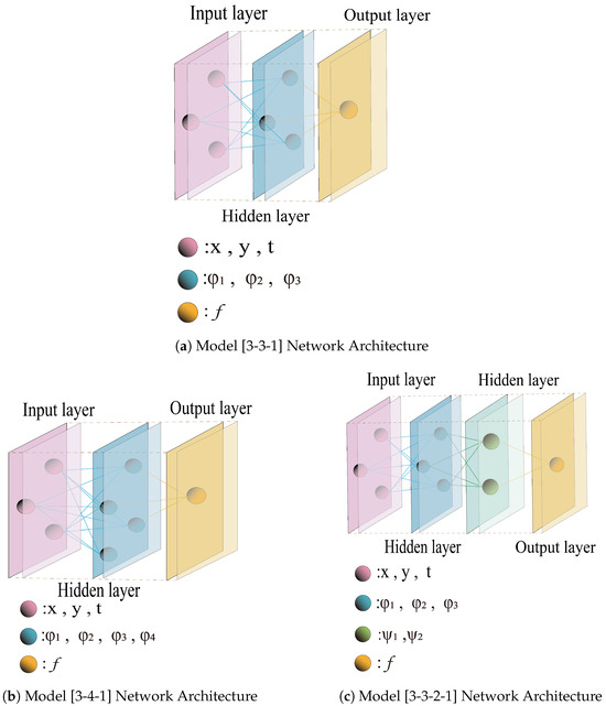
Based on the core research steps described above, this paper utilizes the theoretical framework of the bilinear neural network shown in Figure 1 to construct single-hidden-layer and double-hidden-layer models of the bilinear neural network, respectively.As shown in Figure 2.

Figure 1. Neural Network Model and Algorithm Flowchart.

Figure 2. Single-hidden-layer and double-hidden-layer neural network models constructed in this study.

3. Single-Hidden-Layer Bilinear Neural Network

3.1. Model [3-3-1]-1

To construct a bilinear neural network model, we selected the activation function expression (7) to solve the CBS equation and set the following activation function in the single hidden layer:

$$\begin{array}{c}\hfill \varphi \left({\xi }_1\right)=sech\left({\xi }_1\right)\varphi \left({\xi }_2\right)=sech{\left({\xi }_2\right)}^2\varphi \left({\xi }_3\right)=tanh{\left({\xi }_3\right)}^2\end{array}$$

Substituting this activation function into the analytical form of the network, and by collecting the network outputs and coefficients, we constructed the following trial function:

$$\begin{array}{cc}\hfill f=& b_4+w_{1,u}sech(t{w}_{t,1}+x{w}_{x,1}+y{w}_{y,1}+b_1)+w_{2,u}sech{(t{w}_{t,2}+x{w}_{x,2}+y{w}_{y,2}+b_2)}^2\hfill \\ \hfill & +w_{3,u}tanh{(t{w}_{t,3}+x{w}_{x,3}+y{w}_{y,3}+b_3)}^2\hfill \end{array}$$

(10)

Using this trial function, we also obtained several dimension-reduced auxiliary solutions.

3.1.1. Case 1

Substituting the test function (10) into the bilinear form of the CBS equation and performing symbolic computation using Maple yields the following parameter constraints:

$$\left\{\begin{array}{cc}\hfill b_4& =b_4,w_{1,u}=w_{1,u},w_{2,u}=w_{2,u},w_{3,u}=0,w_{t,1}=w_{t,1},\hfill \\ \hfill w_{t,2}& =w_{t,2},w_{t,3}=w_{t,3},w_{x,1}=0,w_{x,2}=0,w_{x,3}=w_{x,3},\hfill \\ \hfill w_{y,1}& =w_{y,1},w_{y,2}=w_{y,2},w_{y,3}=w_{y,3},\hfill \end{array}\right\}$$

(11)

Substituting (11) back into (10) yields the following approximate solution:

$$\begin{array}{cc}\hfill f=& b_4+w_{1,u}sech(t{w}_{t,1}+y{w}_{y,1}+b_1)+w_{2,u}sech{(t{w}_{t,2}+y{w}_{y,2}+b_2)}^2\hfill \end{array}$$

(12)

We substituted Equation (12) back into the original CBS Equation (2). Using Maple 2023 symbolic computation, the obtained solution served as a dimension-reduced auxiliary solution of the CBS equation.

To more clearly illustrate the spatiotemporal evolution of the solution, we use Maple to assign values to the parameters and generate numerical plots, providing a visual representation of the solution.

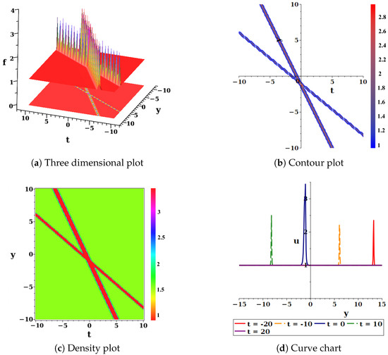
Figure 3 shows a three-dimensional plot displaying the local maximum structure of the auxiliary function $f(y,t)$. The amplitude reached its maximum at $t=0$ and decayed symmetrically toward both sides. Contour plots and heatmaps characterized the contour trajectories and numerical distribution of f. High values concentrated in specific regions. The evolution plots presented profiles at different times. Their peaks and shapes followed specific patterns.

Figure 3. Plots of solution Equation (12), with $b_4=1$, $w_{1,u}=2$, $w_{t,1}=14$, $w_{y,1}=8$, $b_1=10$, $w_{2,u}=1.5$, $w_{t,2}=10$, $w_{y,2}=14$, and $b_2=15$. Here, y denotes the spatial variable, t denotes the temporal variable, and f represents the auxiliary dimension-reduced solution. For brevity, the definitions of variables in all subsequent similar figures are identical to those stated here.

3.1.2. Case 2

To obtain more exact analytical solutions, we continue to use the trial function (10) mentioned above. After substituting (10) into the equation, we obtained different parameter constraints through symbolic computation:

$$\left\{\begin{array}{c}{b}_4=b_4,w_{1,u}=w_{1,u},w_{2,u}=w_{2,u},w_{3,u}=w_{3,u}{w}_{t,1}=w_{t,1},\hfill \\ w_{t,2}=w_{t,2},w_{t,3}=w_{t,3},w_{x,1}=0,w_{x,2}=0,w_{x,3}=0,\hfill \\ w_{y,1}=w_{y,1},w_{y,2}=w_{y,2},w_{y,3}=w_{y,3}.\hfill \end{array}\right\}$$

(13)

Substituting (13) back into (10) yields another approximate solution to the equation:

$$\begin{array}{cc}\hfill f=& b_4+w_{1,u}sech(t{w}_{t,1}+y{w}_{y,1}+b_1)+w_{2,u}sech{(t{w}_{t,2}+y{w}_{y,2}+b_2)}^2\hfill \\ & +w_{3,u}tanh{(t{w}_{t,3}+y{w}_{y,3}+b_3)}^2\hfill \end{array}$$

(14)

SWe substituted Equation (14) back into the original CBS Equation (2). Using Maple symbolic computation, the obtained solution served as a dimension-reduced auxiliary solution of the CBS equation.

As in the previous subsection, to more clearly reveal the spatiotemporal evolution of the solution, we use Maple 2023 to assign values to the parameters and generate numerical plots, thereby providing a visual representation of the solution.

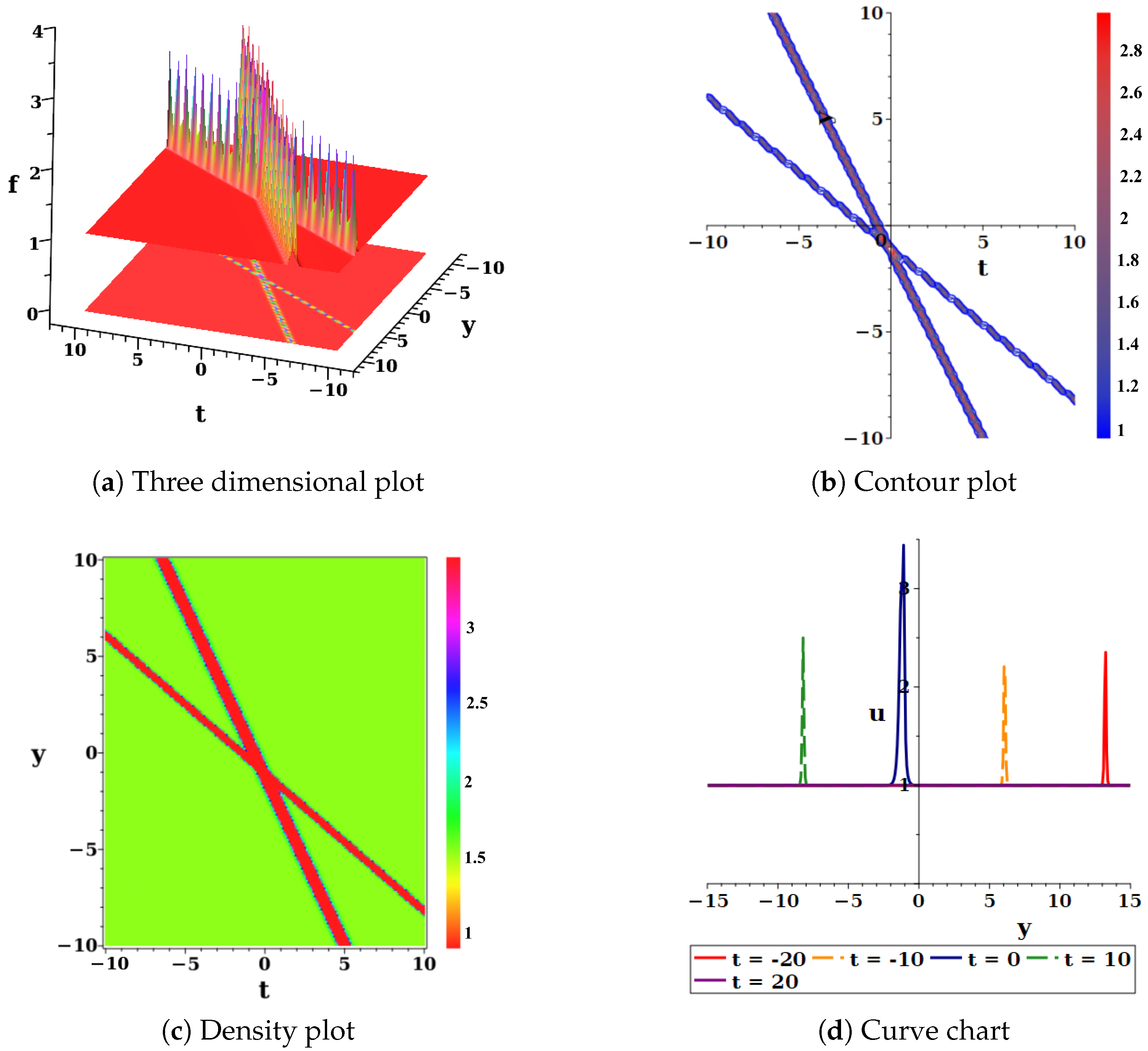
Figure 4 shows a three-dimensional surface plot displaying the spatial form of the auxiliary function f in the spatiotemporal domain. It showed that its values mainly concentrated on intersecting linear ridges, while the background region remained flat. The top-right planar projection and the bottom-left density plot further characterized the geometric topology and numerical distribution trajectories of these characteristic ridges on the t-y plane. The bottom-right time cross-section slices (corresponding to $t=-20,-10,0,10,20)$ revealed the local peak shapes and functional structures of this auxiliary solution along the spatial coordinate y at different times.

Figure 4. Plots of solution Equation (14), with $b_4=1,w_{1,u}=1.5,w_{t,1}=19,w_{y,1}=5,b_1=5$, $w_{2,u}=2,w_{t,2}=20,w_{y,2}=15,b_2=3,w_{3,u}=2,w_{t,3}=6,w_{y,3}=15,b_3=5$.

3.1.3. Case 3

We continue to use this test function to seek more exact solutions. After substituting (10) into the equation, we obtained different parameter constraints through symbolic computation:

$$\left\{\begin{array}{c}{b}_4=b_4,w_{1,u}=0,w_{2,u}=w_{2,u},w_{3,u}=w_{3,u},w_{t,1}=w_{t,1},w_{t,2}=w_{t,2},w_{t,3}=w_{t,3},\hfill \\ w_{x,1}=w_{x,1},w_{x,2}=0,w_{y,1}=w_{y,1},w_{y,2}=w_{y,2},w_{y,3}=w_{y,3}.\hfill \end{array}\right\}$$

(15)

Substituting (15) back into (10) yields another approximate solution to the equation:

$$\begin{array}{cc}\hfill f=& b_4+w_{2,u}sech{(t{w}_{t,2}+y{w}_{y,2}+b_2)}^2+w_{3,u}tanh{(t{w}_{t,3}+y{w}_{y,3}+b_3)}^2\hfill \end{array}$$

(16)

We substituted Equation (16) back into the original CBS Equation (2). Using Maple symbolic computation, the obtained solution served as a dimension-reduced auxiliary solution of the CBS equation.

Similarly, to more clearly reveal the spatiotemporal evolution of the solution, we use Maple 2023 to assign values to the parameters and generate plots, thereby providing a visual representation of the solution.

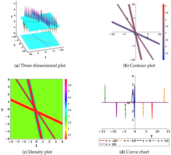
Figure 5 shows a three-dimensional surface plot visually displaying the spatial morphology of the auxiliary function f in the spatiotemporal domain. Its values concentrated markedly on intersecting linear ridges, while the background remained a flat base. The top-right planar projection and the bottom-left density plot further revealed the geometric topology and numerical distribution trajectories of these characteristic ridges on the t-y plane. The bottom-right time cross-section slices (corresponding to $t=-20,-10,0,10,20$) delineated in detail the local peak morphology and functional structure of this auxiliary solution along the spatial coordinate y at different times.

Figure 5. Plots of solution Equation (16), with $b_4=2,w_{2,u}=3,w_{t,2}=9,w_{y,2}=12,b_2=2$, $w_{3,u}=4,w_{t,3}=7,w_{y,3}=15,b_3=1$.

The CBS multi-soliton solutions in References [37,38] are all based on positive-definite exponents and constructions of f, with all soliton components having the same sign. In this paper, the and $tan{h}^2$ terms are coupled in opposite phases through parameter constraints (Equation (16)). This formed a local algebraic structure where peaks and troughs coexisted. The traditional Hirota construction of the CBS equation could hardly generate this structure directly.

3.2. Model [3-4-1]-2

In Section 3.1, symbolic constraints on a specific parameter branch eliminated the dependence of the auxiliary function f on x. This yielded a dimension-reduced auxiliary solution. To explore the diversity of algebraic structures, we retained the single-hidden-layer [3-3-1] architecture in this section. We replaced the activation function combination with one containing $si{n}^2,co{s}^2,tan{h}^2$. The resulting parameter branch did not eliminate the x-direction weight. Thus, we obtained an exact analytical solution containing the spatial variable x. We substituted the trial function back into the Hirota bilinear transformation (Equation (3)). Symbolic computation confirmed that its residual remained identically zero. It strictly satisfied the bilinear form of the original CBS equation. This x-containing solution complemented the dimension-reduced solution in Section 3.1. It demonstrated the regulatory effect of activation functions on the algebraic structure of auxiliary functions.

To construct the bilinear neural network model, we selected activation function expression (7) to solve the CBS equation. In the single hidden layer, we set the following activation functions:

$$\begin{array}{c}\hfill \varphi \left({\xi }_1\right)=sinh{\left({\xi }_1\right)}^2\varphi \left({\xi }_2\right)=cos{\left({\xi }_2\right)}^2\varphi \left({\xi }_3\right)=tanh{\left({\xi }_3\right)}^2\end{array}$$

We substituted this activation function into the analytical form of the network. Through neural network output and coefficient collection, we constructed the following trial function:

$$\begin{array}{cc}\hfill f=b_4& +w_{1,u}sin{\left(t·w_{t,1}+x{w}_{x,1}+y{w}_{y,1}+b_1\right)}^2\hfill \\ \hfill & +w_{2,u}cos{\left(t·w_{t,2}+x{w}_{x,2}+y{w}_{y,2}+b_2\right)}^2\hfill \\ \hfill & +w_{3,u}tanh{\left(t·w_{t,3}+x{w}_{x,3}+y{w}_{y,3}+b_3\right)}^2\hfill \end{array}$$

(17)

Using this trial function, we also derived several exact analytical solutions.

3.2.1. Case 1

We substituted trial function (17) into the bilinear form of the CBS equation. We used Maple for symbolic computation and obtained the following parameter constraints:

$$\left\{\begin{array}{c}{b}_4=b_4,w_{1,u}=w_{1,u},w_{2,u}=0,w_{3,u}=w_{3,u},w_{t,1}=0,\hfill \\ w_{t,2}=w_{t,2},w_{t,3}=4w_{x,1}^2{w}_{y,3},w_{x,1}=w_{x,1},w_{x,2}=w_{x,2},\hfill \\ w_{x,3}=0,w_{y,1}=0,w_{y,2}=w_{y,2},w_{y,3}=w_{y,3}\hfill \end{array}\right\}$$

(18)

We then substituted Equation (18) back into Equation (17) and obtained the following trial solutions:

$$f=b_4+w_{1,u}sin{\left(x{w}_{x,1}+b_1\right)}^2+w_{3,u}tanh{\left(4t{w}_{x,1}^2{w}_{y,3}+y{w}_{y,3}+b_3\right)}^2$$

(19)

We further applied the Hirota transformation (3), namely $u=2{\left(lnf\right)}_x$. We derived the analytical expression (Equation (20)) for the corresponding solution u of the original CBS equation. Symbolic computation verified that this expression strictly satisfied the original CBS equation, with the residual identically zero. Its specific form is given below:

$$u={\displaystyle \frac{4w_{1,u}sin\left(x{w}_{x,1}+b_1\right)w_{x,1}cos\left(x{w}_{x,1}+b_1\right)}{b_4+w_{1,u}sin{\left(x{w}_{x,1}+b_1\right)}^2+w_{3,u}tanh{\left(\left(4t{w}_{x,1}^2+y\right)w_{y,3}+b_3\right)}^2}}$$

(20)

We assigned values to the parameters in Maple 2023 to reveal the spatiotemporal evolution more clearly. We then generated numerical plots to visualize the obtained solution.

The Figure 6 displayed the spatiotemporal structure and numerical distribution of the solution $u(x,t)$ obtained by inverse transformation of the bilinear auxiliary equation. The top-left three-dimensional slice plot visually presented the periodic undulating patterns generated by the wave field u as it evolved over time in the spatiotemporal domain. The top-right planar projection and the bottom-left density plot ($x-t$ plane) further characterized the transverse stripe distribution and periodic structural patterns of this solution in spacetime, accompanied by local phase variations. The bottom-right time cross-section slices (corresponding to $t=0$ and $t=\pi$) revealed in detail the high-frequency, violent oscillation patterns of the wave field u along the spatial coordinate x at specific times. Its amplitude fluctuated between $[-0.4,0.4]$.

Figure 6. Plots of solution Equation (20), with $b_4=2,w_{1,u}=1,w_{x,1}=0.5,b_1=3,w_{3,u}=1$, $w_{y,3}=0.01,b_3=2$. Here, x and t represent the spatial and temporal variables, respectively, and u denotes the exact analytical solution. For brevity, the variable definitions in all subsequent similar figures are identical to those stated here.

3.2.2. Case 2

We continued to use trial function (17) to obtain more exact analytical solutions. We substituted Equation (17) into the equation. Symbolic computation yielded different constraints on the solving parameters:

$$\left\{\begin{array}{c}{b}_4=b_4,w_{1,u}=w_{1,u},w_{2,u}=w_{2,u},w_{3,u}=0,w_{t,1}=4w_{x,2}^2{w}_{y,1},\hfill \\ w_{t,2}=0,w_{t,3}=w_{t,3},w_{x,1}=0,w_{x,2}=w_{x,2},\hfill \\ w_{x,3}=w_{x,3},w_{y,1}=w_{y,1},w_{y,2}=0,w_{y,3}=w_{y,3}\hfill \end{array}\right\}$$

(21)

We then substituted Equation (21) back into Equation (17) and obtained another trial solution of the equation:

$$f=b_4+w_{1,u}sin{\left(4t{w}_{x,2}^2{w}_{y,1}+y{w}_{y,1}+b_1\right)}^2+w_{2,u}cos{\left(x{w}_{x,2}+b_2\right)}^2$$

(22)

We derived the auxiliary function f (Equation (22)) via the Hirota transformation. We calculated the analytical expression for the solution u (Equation (23)). Maple symbolic computation verified that this expression strictly satisfied the original CBS equation, with the residual identically zero. Its specific form is given below:

$$u=-{\displaystyle \frac{4w_{2,u}cos\left(x{w}_{x,2}+b_2\right)w_{x,2}sin\left(x{w}_{x,2}+b_2\right)}{b_4+w_{1,u}sin{\left(\left(4t{w}_{x,2}^2+y\right)w_{y,1}+b_1\right)}^2+w_{2,u}cos{\left(x{w}_{x,2}+b_2\right)}^2}}$$

(23)

To reveal the spatiotemporal evolution more clearly, we assigned parameter values in Maple 2023 and generated numerical plots. This visualized the obtained solution.

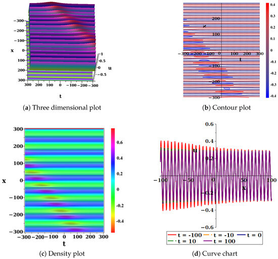
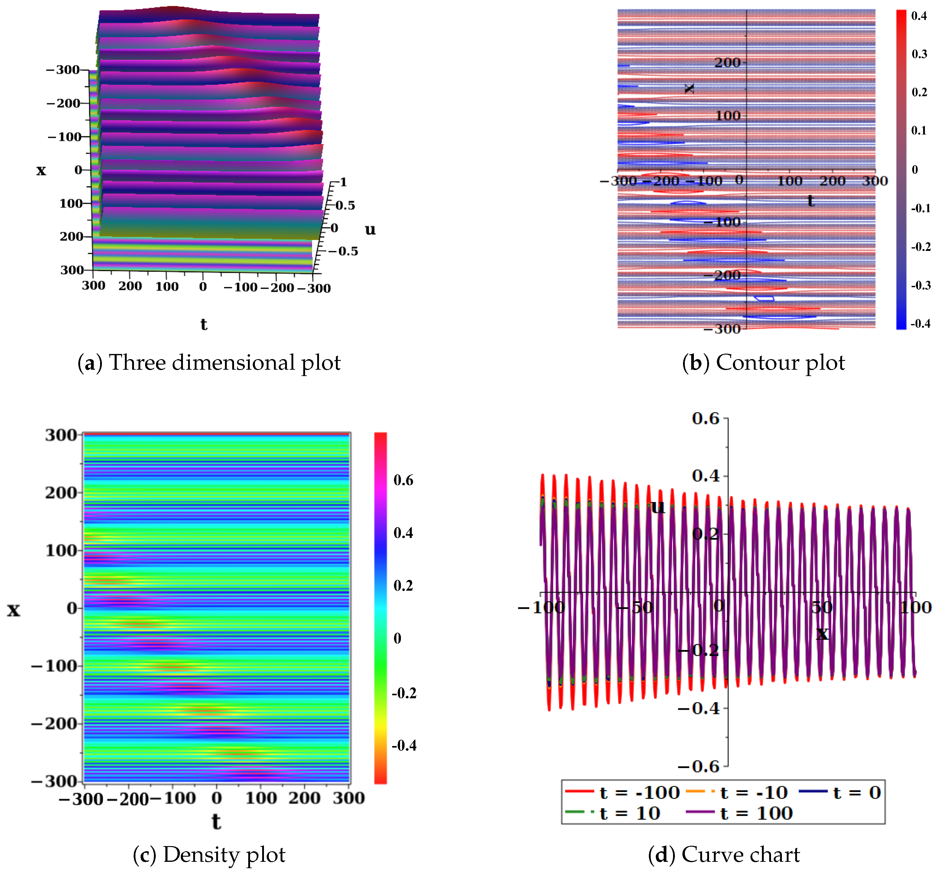
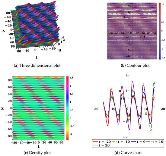
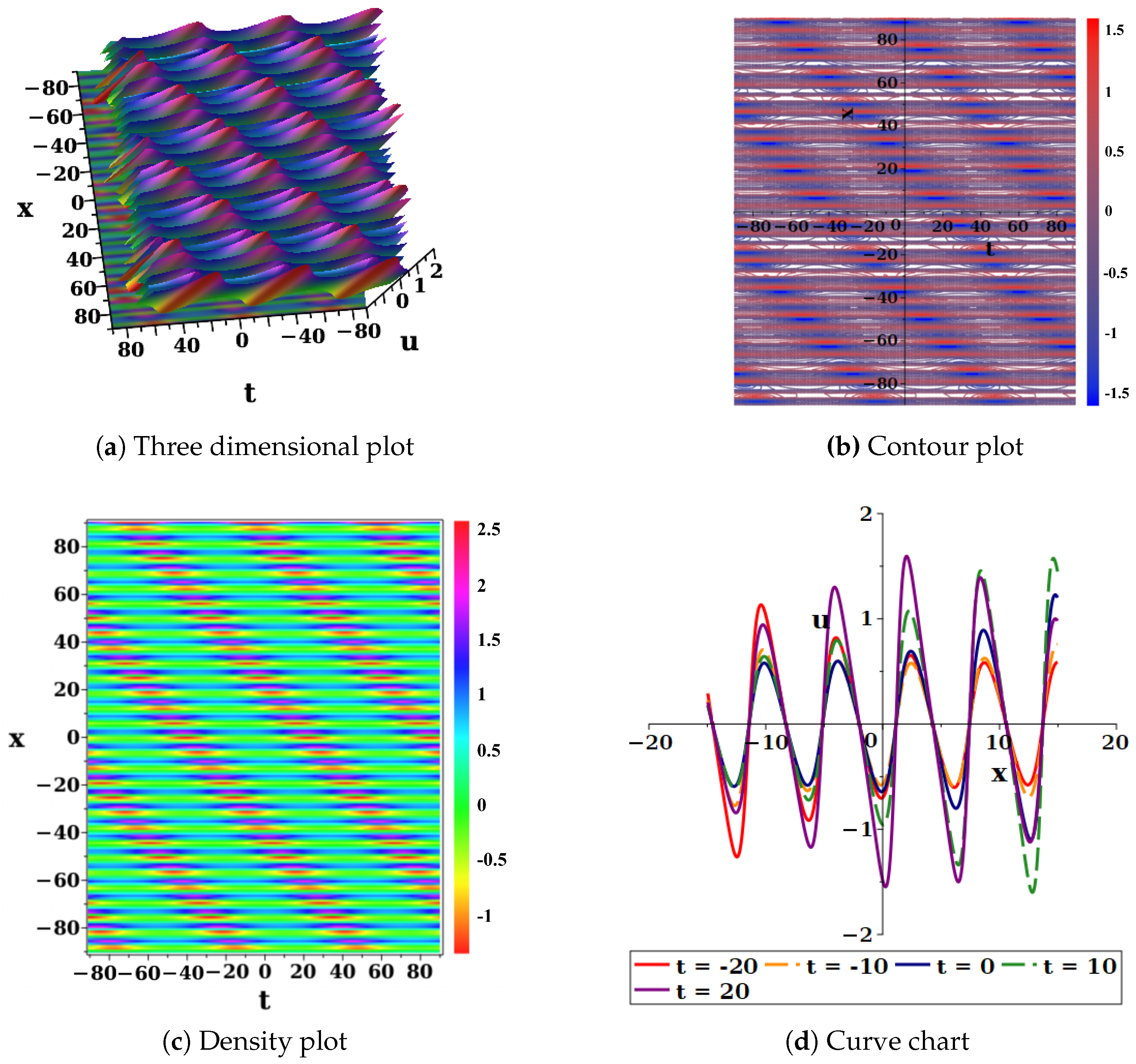
Figure 7 shows a three-dimensional surface plot visually displaying the wave field u as a continuous undulating three-dimensional form in the spatiotemporal domain. Its values showed clear periodic oscillations with the spatial coordinate. The top-right planar projection and the bottom-left spatiotemporal density plot ($x-t$ plane) further characterized the transverse periodic stripe distribution of this wave field. They clearly showed the phase shift and propagation trajectory of the wave, with values roughly between −1.5 and 2.5. The bottom-right time cross-section slices (corresponding to $t=-20,-10,0,20$) revealed in detail the high-frequency oscillation patterns of the wave field u along the spatial coordinate x at different times. Its amplitude peaks exhibited a non-constant evolution over time.

Figure 7. Plots of solution Equation (23), with $b_4=0.3,w_{1,u}=1,w_{x,2}=0.5,b_2=1,w_{2,u}=1,w_{x,1}=0.05,w_{y,1}=0.05,b_1=2$.

3.2.3. Case 3

We continued to substitute trial function (17) into the bilinear form of the CBS equation. We used Maple for symbolic computation. We then obtained the following parameter constraints:

$$\left\{\begin{array}{c}{b}_4=b_4,w_{1,u}=w_1,w_{2,u}=w_2,w_{3,u}=0,w_{t,1}=0,w_{t,2}=4w_{x,1}^2{w}_{y,2},w_{t,3}=w_{t,3},\hfill \\ w_{x,1}=w_{x,1},w_{x,2}=0,w_{x,3}=w_x,w_{y,1}=0,w_{y,2}=w_y,w_{y,3}=w_{y,3}\hfill \end{array}\right\}$$

(24)

We then substituted Equation (24) back into Equation (17) and obtained the following trial solution:

$$f=b_4+w_{1,u}sin{\left(x{w}_{x,1}+b_1\right)}^2+w_{2,u}cos{\left(4t{w}_{x,1}^2{w}_{y,2}+y{w}_{y,2}+b_2\right)}^2$$

(25)

Similarly, we continued to apply the Hirota transformation. We derived the analytical expression for the solution u (Equation (26)) from the auxiliary function f. Symbolic computation verified that this expression strictly satisfied the original CBS equation, with the residual identically zero. Its specific form is given below:

$$u={\displaystyle \frac{4w_{1,u}sin\left(x{w}_{x,1}+b_1\right)w_{x,1}cos\left(x{w}_{x,1}+b_1\right)}{b_4+w_{1,u}sin{\left(x{w}_{x,1}+b_1\right)}^2+w_{2,u}cos{\left(\left(4t{w}_{x,1}^2+y\right)w_{y,2}+b_2\right)}^2}}$$

(26)

To reveal the spatiotemporal evolution of the solution more clearly, we assigned values to the parameters in Maple 2023. We then generated numerical plots. These plots visualized the obtained solution directly.

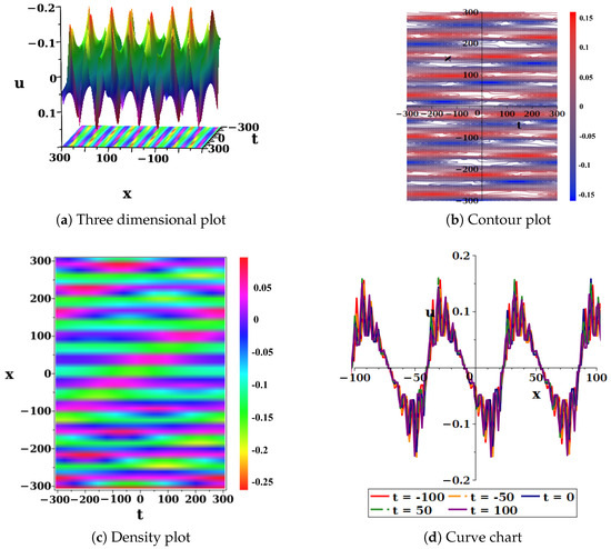
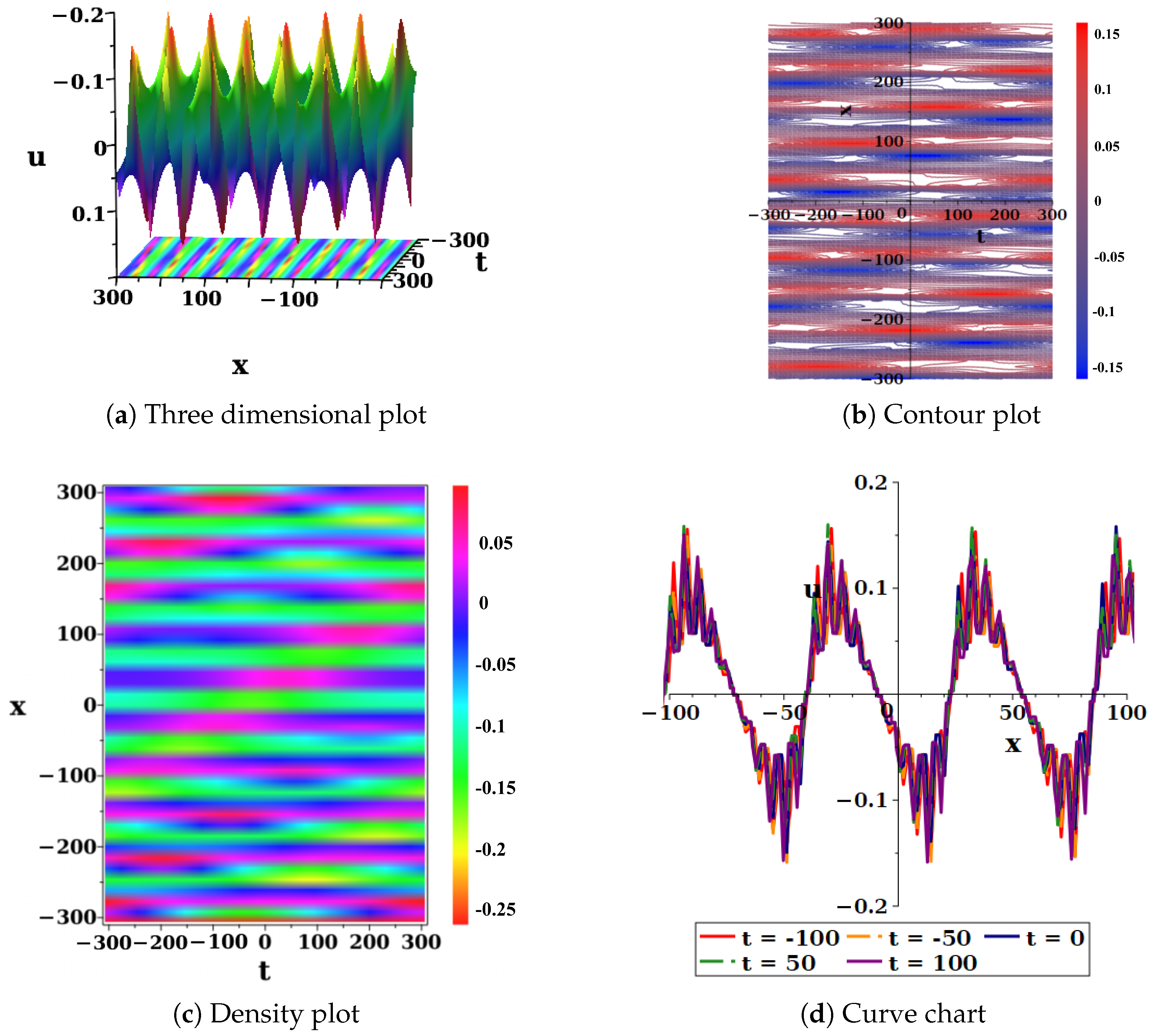
Figure 8 shows a subplot visually presenting the three-dimensional undulating form of the wave field within a specific local region. It clearly showed a regular and dense alternating peak-valley structure. The top-right and bottom-left subplots (planar projection and spatiotemporal density plot) further characterized the overall distribution of this solution across a broad spatiotemporal domain. They exhibited complex transverse periodic stripes and phase shift trajectories, with values fluctuating between −0.25 and 0.15. The bottom-right time cross-section slices (corresponding to $t=-100,-50,0,50,100$) revealed in detail the violent high-frequency oscillation patterns of the wave field u along the spatial coordinate x at several specific times. Its amplitude peaks showed a certain evolutionary pattern over time.

Figure 8. Plots of solution Equation (26), with $b_4=0.3,w_{1,u}=1,w_{y,2}=0.5,b_2=2,w_{2,u}=1$, $w_{x,1}=0.05,b_1=2$.

3.3. Model [3-4-1]

To construct more bilinear neural network models, we further tested different activation function expressions. We selected activation function expression (8) to solve the CBS equation. To obtain different types of analytical structures for the auxiliary function, we tried replacing the activation function. We then reset new activation functions in the single hidden layer as follows:

$$\begin{array}{c}\hfill \varphi \left({\xi }_1\right)=sinh\left({\xi }_1\right)\varphi \left({\xi }_2\right)=tanh{\left({\xi }_2\right)}^2\varphi \left({\xi }_3\right)=tanh{\left({\xi }_3\right)}^2\varphi \left({\xi }_4\right)=csch{\left({\xi }_4\right)}^2\end{array}$$

By substituting this trial function into the analytical form of the network, we constructed the following trial function:

$$\begin{array}{cc}\hfill f=b_5& +w_{1,u}sinh(t·w_{t,1}+x{w}_{x,1}+y{w}_{y,1}+b_1)\hfill \\ \hfill & +w_{2,u}tanh{(t·w_{t,2}+x{w}_{x,2}+y{w}_{y,2}+b_2)}^2\hfill \\ \hfill & +w_{3,u}tanh{(t·w_{t,3}+x{w}_{x,3}+y{w}_{y,3}+b_3)}^2\hfill \\ \hfill & +w_{4,u}csch{(t·w_{t,4}+x{w}_{x,4}+y{w}_{y,4}+b_4)}^2\hfill \end{array}$$

(27)

Using this trial function, we obtained several dimension-reduced auxiliary solutions, as follows:

3.3.1. Case 1

Substituting the test function (27) into the bilinear form of the CBS equation and performing symbolic calculations in Maple yields the following parameter constraint:

$$\left\{\begin{array}{c}{w}_{4,u}=w_{4,u},b_5=b_5,w_{1,u}=0,w_{2,u}=w_{2,u},w_{3,u}=w_{3,u},w_{t,1}=w_{t,1},w_{t,2}=w_{t,2},\hfill \\ w_{t,3}=w_{t,3},w_{t,4}=w_{t,4},w_{x,1}=w_{x,1},w_{x,2}=0,w_{x,3}=0,w_{x,4}=0,w_{y,1}=w_{y,1},\hfill \\ w_{y,2}=w_{y,2},w_{y,3}=w_{y,3},w_{y,4}=w_{y,4}\hfill \end{array}\right\}$$

(28)

Substituting (28) back into (27) yields the following approximate solution:

$$\begin{array}{cc}\hfill f=& b_5+w_{2,u}tanh{(t{w}_{t,2}+y{w}_{y,2}+b_2)}^2+w_{3,u}tanh{(t{w}_{t,3}+y{w}_{y,3}+b_3)}^2\hfill \\ & +w_{4,u}csch{(t{w}_{t,4}+y{w}_{y,4}+b_4)}^2\hfill \end{array}$$

(29)

We substituted Equation (29) back into the original CBS Equation (2). Using Maple symbolic computation, we obtained a dimension-reduced auxiliary solution of the CBS equation.

To more clearly illustrate the spatiotemporal evolution of the solution, we use Maple 2023 to assign values to the parameters and generate numerical plots, thereby providing a visual representation of the solution.

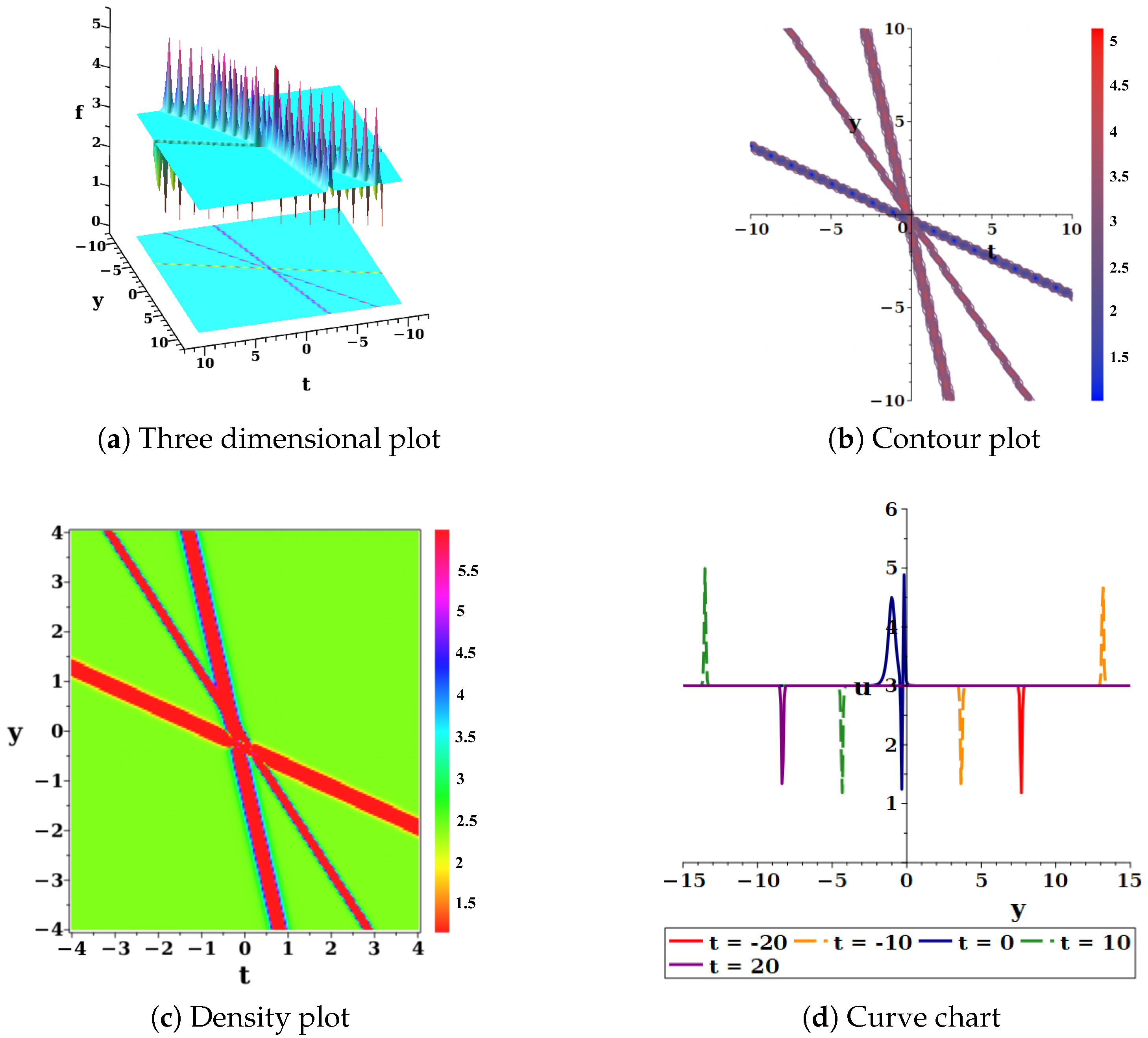
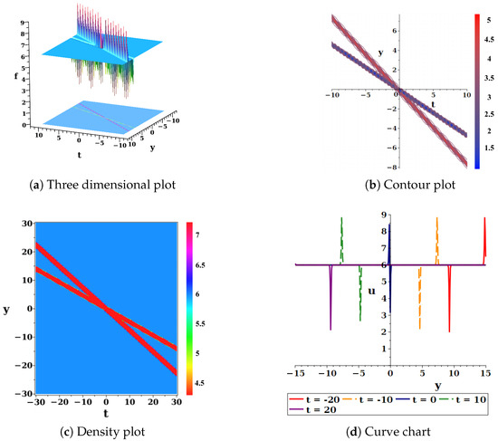
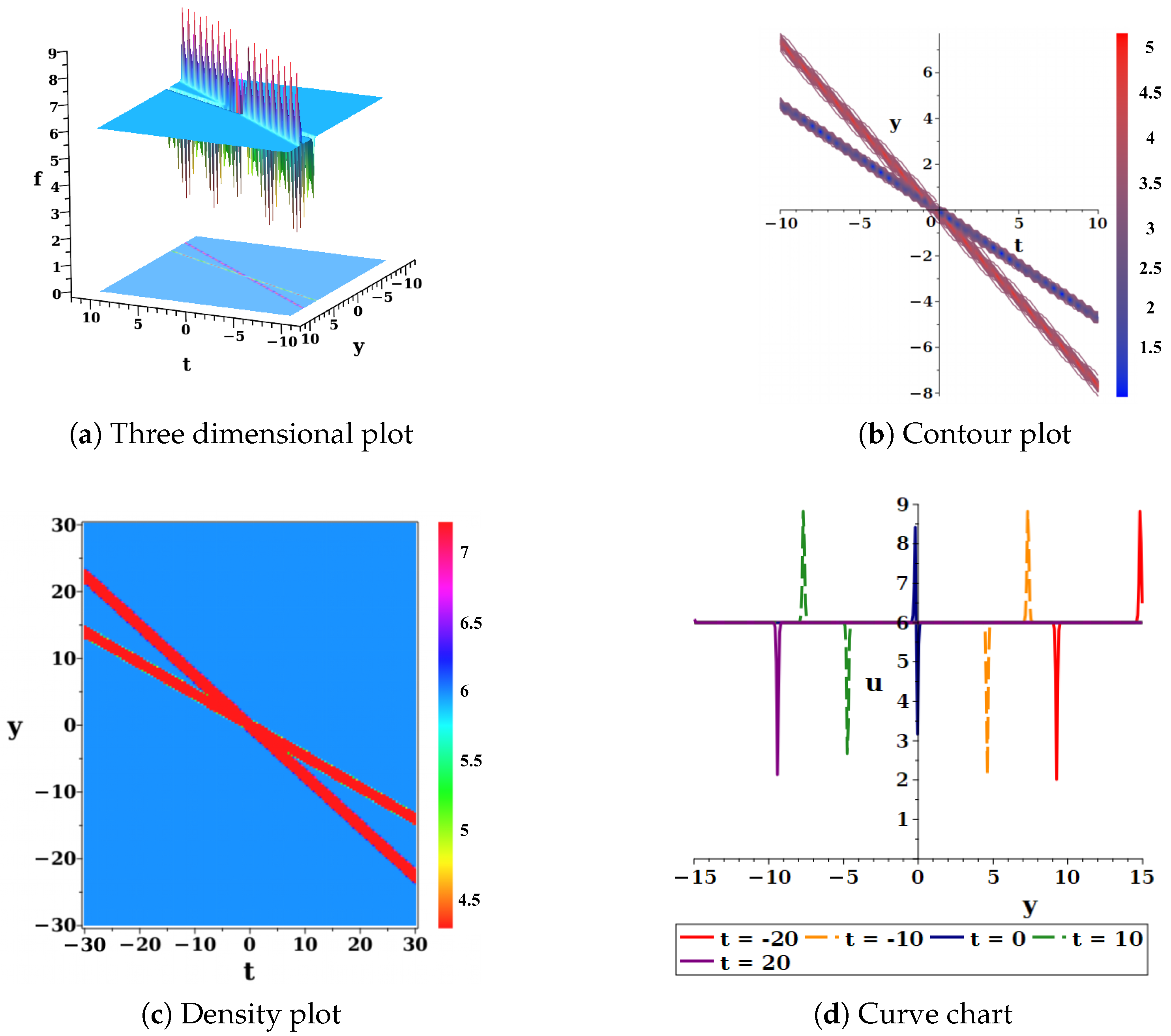
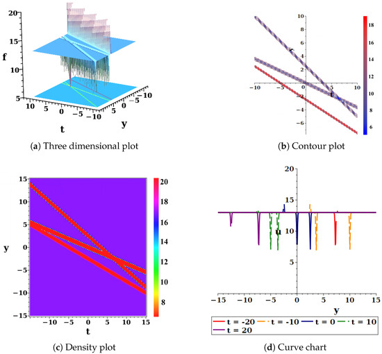
Figure 9 shows a 3D surface plot displaying the spatial form of the auxiliary function f in the spatiotemporal domain. Its values concentrated markedly on several intersecting linear ridges. The background remained flat. The top-right planar projection and the bottom-left density plot further characterized the geometric topology and numerical distribution trajectories of these ridges on the t-y plane. The bottom-right time cross-section slices (t = −20, −10, 0, 10, 20) revealed in detail the local peak morphology and functional structure of this auxiliary solution along the spatial coordinate y at different times.

Figure 9. Plots of solution Equation (29), with $b_5=1,w_{2,u}=6,w_{t,2}=9,w_{y,2}=12,b_2=-30$, $w_{3,u}=6,w_{t,3}=4,w_{y,3}=11,b_3=0,w_{4,u}=0.9,w_{t,4}=6,w_{y,4}=12,b_4=30$.

3.3.2. Case 2

To obtain more dimension-reduced auxiliary analytical solutions, we continue to use the trial function (27) as in the previous model. After substituting it into the equation, we obtained different parameter constraints through symbolic computation:

$$\left\{\begin{array}{c}{w}_{4,u}=0,b_5=b_5,w_{1,u}=w_{1,u},w_{2,u}=w_{2,u},w_{3,u}=w_{3,u},w_{t,1}=w_{t,1},w_{t,2}=w_{t,2},\hfill \\ w_{t,3}=w_{t,3},w_{t,4}=w_{t,4},w_{x,1}=0,w_{x,2}=0,w_{x,3}=0,w_{x,4}=w_{x,4},w_{y,1}=w_{y,1},\hfill \\ w_{y,2}=w_{y,2},w_{y,3}=w_{y,3},w_{y,4}=w_{y,4}\hfill \end{array}\right\}$$

(30)

Substituting (30) back into (27) yields another approximate solution to the equation:

$$\begin{array}{cc}\hfill f=& b_5+w_{1,u}sinh(t{w}_{t,1}+y{w}_{y,1}+b_1)+w_{2,u}tanh{(t{w}_{t,2}+y{w}_{y,2}+b_2)}^2\hfill \\ & +w_{3,u}tanh{(t{w}_{t,3}+y{w}_{y,3}+b_3)}^2\hfill \end{array}$$

(31)

We substituted Equation (31) back into the original CBS Equation (2). Using Maple symbolic computation, we obtained a dimension-reduced auxiliary solution of the CBS equation.

As in the previous subsection, to more clearly illustrate the spatiotemporal evolution of the solution, we used Maple 2023 software to assign values to the parameters and generate numerical plots, thereby providing a visual representation of the solution.

Figure 10 shows the extreme numerical structural characteristics of the dimension-reduced solution $f(y,t)$ for the bilinear auxiliary equation in a local region. The top-left three-dimensional surface plot visually presented an extremely narrow, high-amplitude pulse-like spike of f within a specific local spatiotemporal domain. The top-right local planar projection and the bottom-left density plot further depicted the contour gradient variations and sharp numerical transitions around the spike extremum. The bottom-right time cross-section slices (corresponding to $t=-2,-1,0,1,2$) revealed in detail the sharp local peak morphology and functional structure of this local solution along the spatial coordinate y at different times.

Figure 10. Plotsof solution Equation (31), with $b_5=4,w_{1,u}=5,w_{t,1}=4,w_{y,1}=6,b_1=6,w_{3,u}=1$, $w_{t,3}=4,w_{y,3}=7,b_3=5,w_{2,u}=2,w_{t,2}=5,w_{y,2}=3,b_2=4.$

Wazwaz’s [37,38] multi-soliton solutions do not contain unbounded functions, whereas this paper introduces the sinh activation function (Equation (31)) to obtained a mixed function structure superimposed on a nonzero background. This solution differed from the structure Ma et al. [33] obtained by parameter complexification. We constructed it entirely in the real parameter space. It therefore had a more intuitive algebraic structure.

3.3.3. Case 3

We continue to use this test function to seek more exact solutions. After substituting (27) into the equation, we obtained different parameter constraints through symbolic computation:

$$\left\{\begin{array}{c}{w}_{4,u}=0,b_5=b_5,w_{1,u}=0,w_{2,u}=w_{2,u},w_{3,u}=w_{3,u},w_{t,1}=w_{t,1},w_{t,2}=w_{t,2},\hfill \\ w_{t,3}=w_{t,3},w_{t,4}=w_{t,4},w_{x,1}=w_{x,1},w_{x,2}=0,w_{x,3}=0,w_{x,4}=w_{x,4},\hfill \\ w_{y,1}=w_{y,1},w_{y,2}=w_{y,2},w_{y,3}=w_{y,3},w_{y,4}=w_{y,4}\hfill \end{array}\right\}$$

(32)

Substituting (32) back into (27) yields another approximate solution to the equation:

$$\begin{array}{cc}\hfill f=& b_5+w_{2,u}tanh{(t{w}_{t,2}+y{w}_{y,2}+b_2)}^2+w_{3,u}tanh{(t{w}_{t,3}+y{w}_{y,3}+b_3)}^2\hfill \end{array}$$

(33)

Similarly, we substituted Equation (33) back into the original CBS Equation (2). The resulting solution served as a dimension-reduced auxiliary solution of the CBS equation.

Similarly, to more clearly illustrate the spatiotemporal evolution of the solution, we use Maple 2023 software to assign values to the parameters and generate numerical plots, thereby providing a visual representation of the solution.

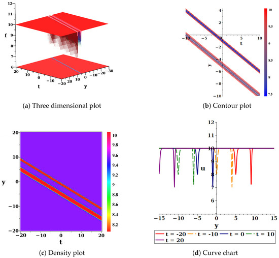
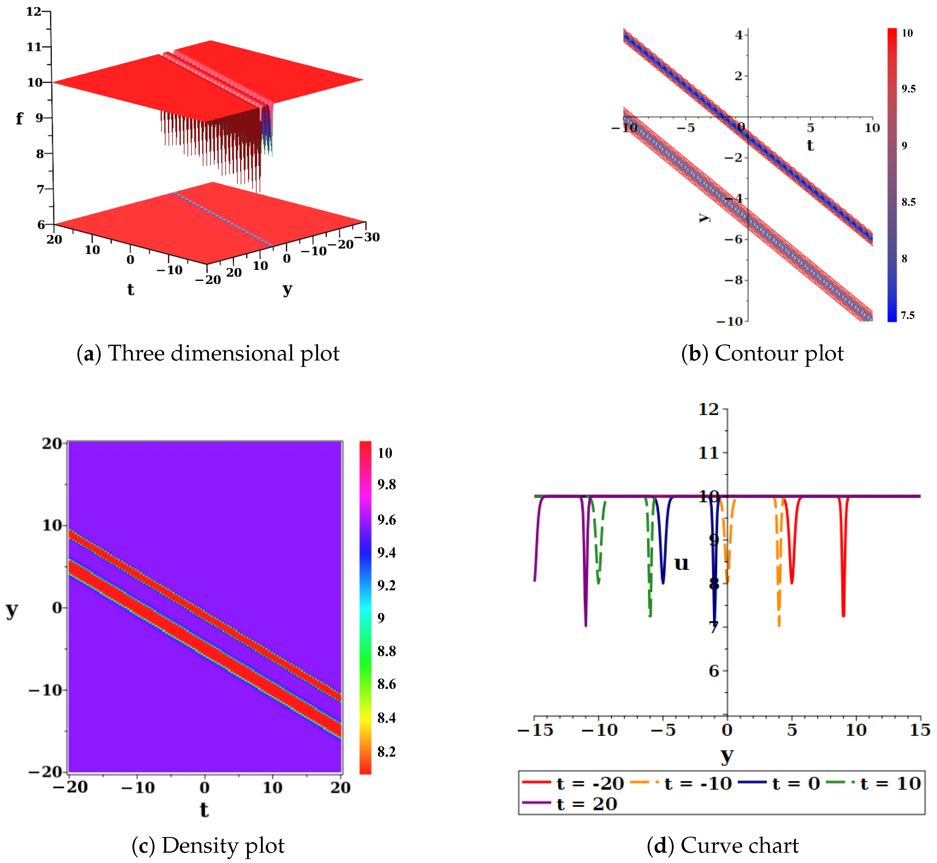
Figure 11 shows a 3D surface plot displaying the spatial form of f in the spatiotemporal domain. It appeared as local downward linear grooves on a flat high-value base. The top-right planar projection and the bottom-left density plot further characterized the geometric topology and numerical distribution trajectories of these linear grooves on the $t-y$ plane. The color bar indicated values from about 7.5 to 10. The bottom-right time cross-section slices ($t=-20,-10,0,10,20$) revealed in detail the local depression morphology and functional structure of this auxiliary solution along the spatial coordinate y at different times.

Figure 11. Plots of solution Equation (33), with $b_5=5,w_{2,u}=3,w_{t,2}=4,w_{y,2}=8,b_2=8,w_{3,u}=2$, $w_{t,3}=2,w_{y,3}=4,b_3=20.$

4. Double-Hidden-Layer Bilinear Neural Network

4.1. Model [3-3-2-1]

Unlike the single-hidden-layer neural network architectures discussed in the previous two sections, in this section we present a double-hidden-layer neural network architecture. We selected the activation function given by Equation (9) to solve the equations, and in the double-hidden-layer architecture, we set the activation functions as follows:

$$\begin{array}{cc}\hfill & \varphi \left({\xi }_4\right)=e^{{\xi }_4}\varphi \left({\xi }_5\right)=WeierstrassP\left({\xi }_5\right)\hfill \\ \hfill & \varphi \left({\xi }_1\right)=sech\left({\xi }_1\right)\varphi \left({\xi }_2\right)=tanh\left({\xi }_2\right)\varphi \left({\xi }_3\right)=sech\left({\xi }_3\right)\hfill \end{array}$$

Substituting this function into the analytical form of the network, we construct the following test function:

$$\begin{array}{cc}\hfill f=& w_{4,u}{e}^{w_{1,u}sech(x{w}_{x,1}+y{w}_{y,1}+t{w}_{t,1}+b_1)}·e^{w_{2,u}tanh(x{w}_{x,2}+y{w}_{y,2}+t{w}_{t,2}+b_2)}\hfill \\ & ·e^{w_{3,u}sech(x{w}_{x,3}+y{w}_{y,3}+t{w}_{t,3}+b_3)+b_4}\hfill \\ \hfill & +w_{5,u}WeierstrassP(w_{1,u}sech(x{w}_{x,1}+y{w}_{y,1}+t{w}_{t,1}+b_1)\hfill \\ & +w_{2,u}tanh(x{w}_{x,2}+y{w}_{y,2}+t{w}_{t,2}+b_2)\hfill \\ \hfill & +w_{3,u}sech(x{w}_{x,3}+y{w}_{y,3}+t{w}_{t,3}+b_3)+b_5,1,1)+b_6\hfill \end{array}$$

(34)

Using this test function, we obtained the following exact analytical solutions.

4.1.1. Case 1

Substituting the test function (34) into the bilinear form of the equation, and after collecting the neural network outputs and coefficients, we obtained the following parameter constraints through symbolic computation:

$$\left\{\begin{array}{c}{b}_6=b_6,w_{1,u}=w_{1,u},w_{2,u}=w_{2,u},w_{3,u}=0,w_{4,u}=w_{4,u},w_{5,u}=w_{5,u},w_{t,1}=w_{t,1},\hfill \\ w_{t,2}=w_{t,2},w_{t,3}=w_{t,3},w_{x,1}=0,w_{x,2}=0,w_{x,3}=w_{x,3},w_{y,1}=w_{y,1},\hfill \\ w_{y,2}=w_{y,2},w_{y,3}=w_{y,3}.\hfill \end{array}\right\}$$

(35)

As with the previous two models, we substituted Equation (35) back into the original CBS Equation (2). The resulting solution was a dimension-reduced auxiliary solution of the CBS equation.

$$\begin{array}{cc}\hfill f=& w_{4,u}{e}^{(w_{1,u}sech(t{w}_{t,1}+y{w}_{y,1}+b_1)+w_{2,u}tanh(t{w}_{t,2}+y{w}_{y,2}+b_2)+b_4)}\hfill \\ & +w_{5,u}WeierstrassP(w_{1,u}sech(t{w}_{t,1}+y{w}_{y,1}+b_1)\hfill \\ & +w_{2,u}tanh(t{w}_{t,2}+y{w}_{y,2}+b_2)+b_{5}1,1)+b_6\hfill \end{array}$$

(36)

As with the previous two models, substituting Equation (36) back into the original CBS Equation (2) yields a residual that is always zero; therefore, this solution is an exact analytical solution for dimension reduction of the CBS equation.

To more clearly illustrate the spatiotemporal evolution of the solution, we used Maple 2023 to assign values to the parameters and generate numerical plots, thereby providing a visual representation of the solution.

Figure 12 shows the specific mathematical structure of the dimension-reduced solution $f(y,t)$ for the bilinear auxiliary equation. The top-left three-dimensional surface plot visually presented the spatial form of the auxiliary function f in the spatiotemporal domain. It appeared as local downward linear grooves on a flat high-value base. The top-right planar projection and the bottom-left density plot further characterized the geometric topology and numerical distribution trajectories of these linear grooves on the $t-y$ plane. The color bar showed values ranging from about 7.5 to 10. The bottom-right time cross-section slices (corresponding to $t=-20,-10,0,10,20$) revealed in detail the local depression morphology and functional structure of this auxiliary solution along the spatial coordinate y at different times.

Figure 12. Plotsof solution Equation (36), with $w_{5,u}=3,w_{2,u}=3,w_{1,u}=2,w_{4,u}=2,w_{y,1}=8$, $w_{t,1}=5,b_1=2,w_{y,2}=8,w_{t,2}=5,b_2=3,b_4=4,b_5=4000,b_6=4000.$

All solutions by Wazwaz [37,38] and Najafi et al. They are limited to elementary functions and do not involve elliptic functions. This paper is the first to introduce the Weierstrass P elliptic function as an activation function in the CBS equation (Equation (36)), We derived a hybrid auxiliary function structure that coupled exponential and elliptic functions, marking a substantial expansion of the solution space of the CBS equation at the level of function families.

4.1.2. Case 2

To obtain more precise analytical solutions, we continue to use the test function (34). After substituting it into the equation, we obtained different parameter constraints through symbolic computation:

$$\left\{\begin{array}{c}{b}_6=b_6,w_{1,u}=0,w_{2,u}=w_{2,u},w_{3,u}=0,w_{4,u}=w_{4,u},w_{5,u}=w_{5,u},w_{t,1}=w_{t,1},\hfill \\ w_{t,2}=w_{t,2},w_{t,3}=w_{t,3},w_{x,1}=w_{x,1},w_{x,2}=0,w_{x,3}=w_{x,3},w_{y,1}=w_{y,1},\hfill \\ w_{y,2}=w_{y,2},w_{y,3}=w_{y,3}\hfill \end{array}\right\}$$

(37)

Substituting (37) back into (34) yields an exact analytical solution to the equation:

$$\begin{array}{cc}\hfill f=& w_{4,u}{e}^{(w_{2,u}tanh(y{w}_{y,2}+t{w}_{t,2}+b_2)+b_4)}\hfill \\ & +w_{5,u}WeierstrassP(w_{2,u}tanh(y{w}_{y,2}+t{w}_{t,2}+b_2)+b_5,1,1)+b_6\hfill \end{array}$$

(38)

Similarly, we substituted Equation (38) back into the original CBS Equation (2). We obtained a dimension-reduced auxiliary solution of the CBS equation.

To more clearly illustrate the spatiotemporal evolution of the solution, we use Maple 2023 to assign values to the parameters and generate numerical plots, thereby providing a visual representation of the solution.

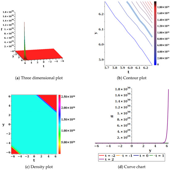
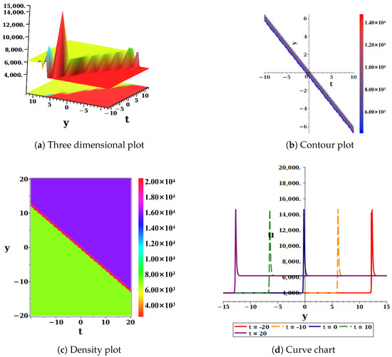
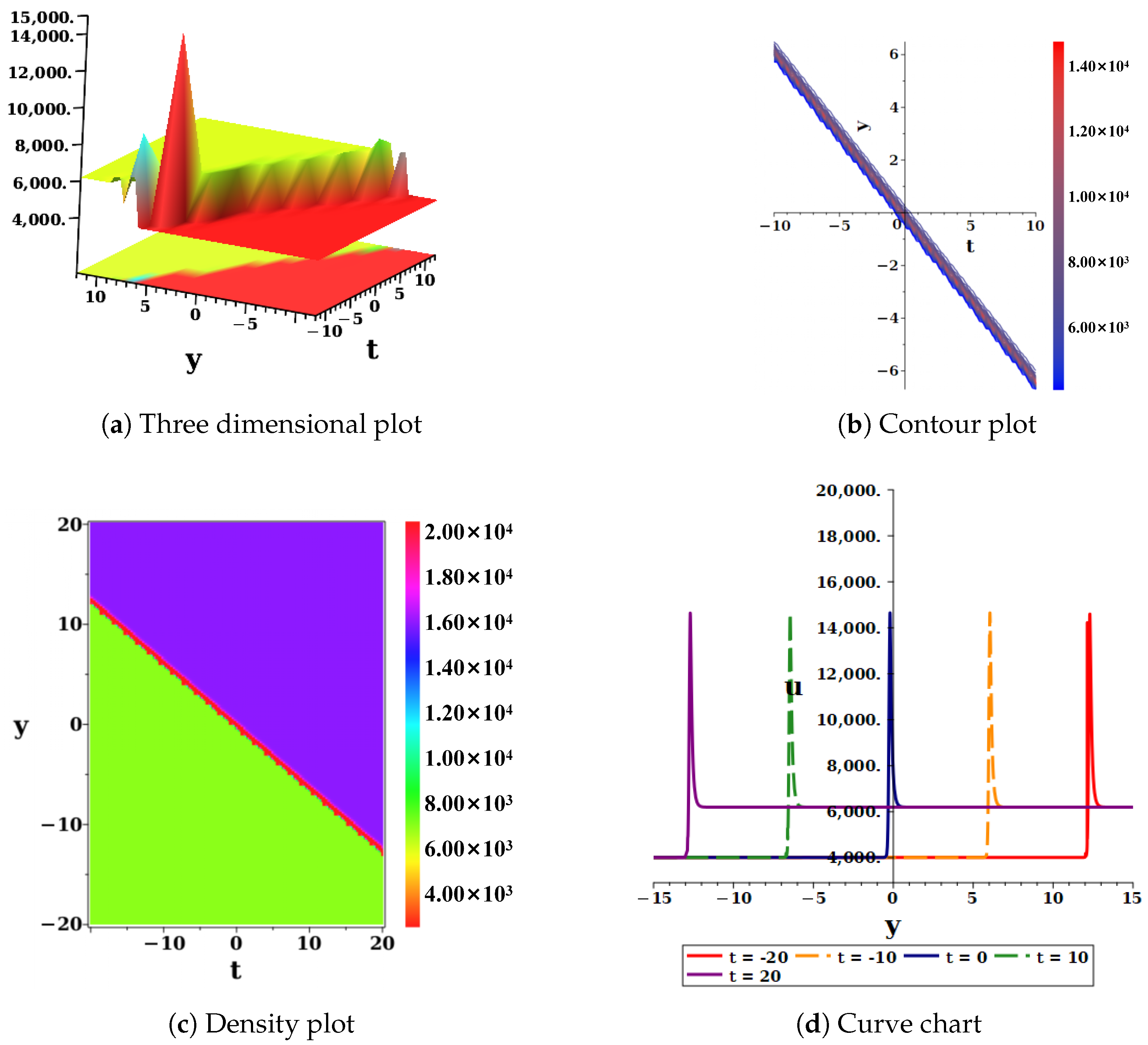
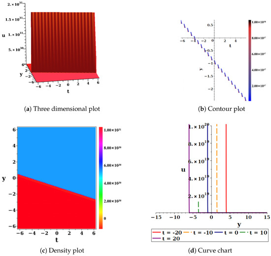
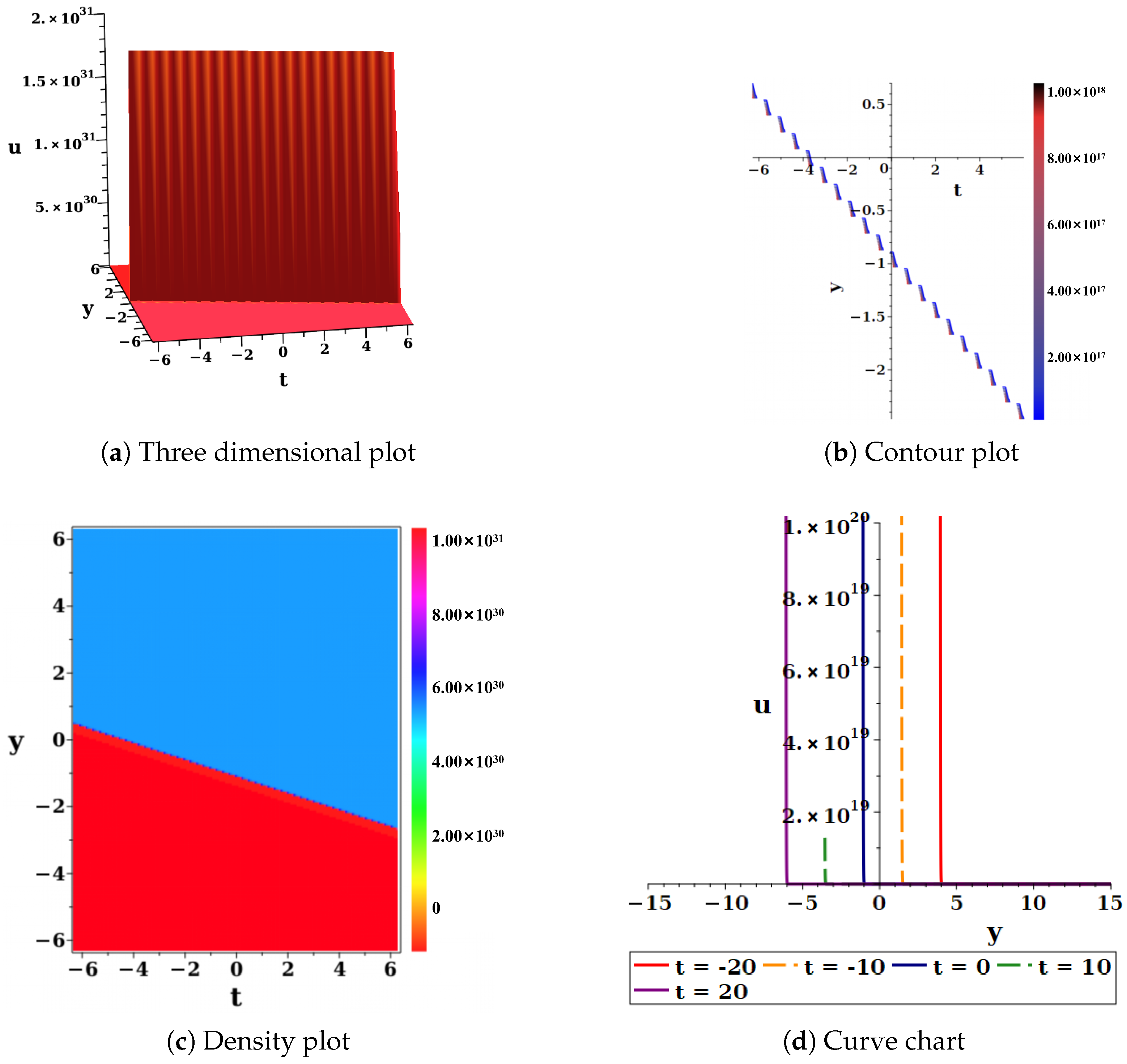
Figure 13 shows a 3D surface plot showing that a steep linear boundary divided the function f in the $y-t$ plane into two parts. The two sides differed greatly in numerical magnitude, up to ${10}^{31}$. The top-right planar projection and the bottom-left density plot further characterized the geometric topology and contour distribution of this sharp transition interface on the plane. The bottom-right time cross-section slices $(t=-20,-10,0,10,20)$ revealed in detail the local extremum points and abrupt morphological changes of this auxiliary solution along the spatial coordinate y as time evolved.

Figure 13. Plots of solution Equation (38), with $w_{5,u}=1,w_{2,u}=2,w_{4,u}=3,w_{y,2}=20,w_{t,2}=5$, $b_2=9,b_3=3,b_4=5,b_5=2,b_6=14.$

The respiron solution by Ma et al. [33] is essentially a combination of elementary functions, whereas this solution belongs to the category of elliptic functions and has no precedent in the existing literature on the CBS equation.In subplots (a) three-dimensional plot, (b) contour plot, and (c) density plot, the colors represent the magnitude of the auxiliary function f, as indicated by the colorbars. In subplot (d) curve chart, the differently colored curves represent the spatial profiles $f\left(y\right)$ at different time instants, corresponding to the legend at the bottom.

4.1.3. Case 3

To expand the solution space, we continue to use this trial function. Substituting it into the equation and performing symbolic calculations yields several sets of distinct parameter constraints:

$$\left\{\begin{array}{c}{b}_6=b_6,w_{1,u}=w_{1,u},w_{2,u}=0,w_{3,u}=0,w_{4,u}=w_{4,u},w_{5,u}=w_{5,u},w_{t,1}=w_{t,1},\hfill \\ w_{t,2}=w_{t,2},w_{t,3}=w_{t,3},w_{x,1}=0,w_{x,2}=w_{x,2},w_{x,3}=w_{x,3},w_{y,1}=w_{y,1},\hfill \\ w_{y,2}=w_{y,2},w_{y,3}=w_{y,3}\hfill \end{array}\right\}$$

(39)

Substituting (39) back into (34) yields an exact analytical solution to the equation:

$$\begin{array}{cc}\hfill f=& w_{4,u}{e}^{(w_{1,u}sech(y{w}_{y,1}+t{w}_{t,1}+b_1)+b_4)}\hfill \\ & +w_{5,u}WeierstrassP(w_{1,u}sech(y{w}_{y,1}+t{w}_{t,1}+b_1)+b_5,1,1)+b_6\hfill \end{array}$$

(40)

Similarly, we substituted Equation (40) back into the original CBS Equation (2). We obtained a dimension-reduced auxiliary solution of the CBS equation.

To facilitate observation of the evolution of the solution, we use Maple 2023 to set specific values for the parameters and generate corresponding graphs for visualization.

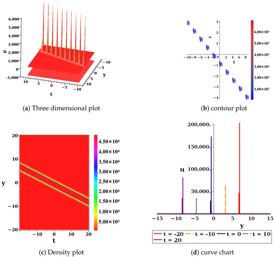
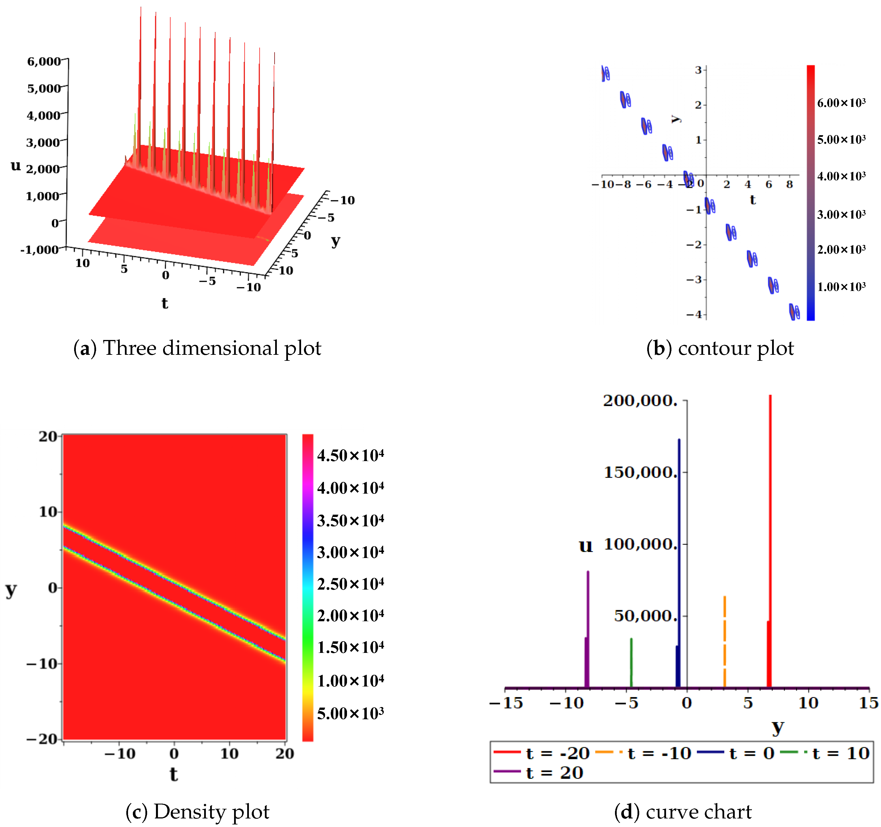
Figure 14 shows a 3D surface plot visually showing periodically arranged isolated sharp peaks of f in the spatiotemporal domain. The whole field rested on a relatively high background base. The top-right planar projection and the bottom-left density plot further characterized the geometric distribution and numerical transition trajectories of these discrete pulse lattices on the t-y plane. The color bar indicated values varying sharply from about $5.00\times {10}^3$ to $4.50\times {10}^4$. The bottom-right time cross-section slices (corresponding to $t=-20,-10,0,10,20$) revealed in detail the independent towering peak morphology of this auxiliary solution along the spatial coordinate y at different times.

Figure 14. Plots of solution Equation (40), with $w_{4,u}=2,w_{1,u}=2,w_{t,1}=1.5,w_{y,1}=4,b_1=3,b_4=1$, $w_{5,u}=1,b_5=1,b_6=9.$

All known solutions in References [37,38] are globally defined functions. This solution “truncates” the biperiodic behavior of the Weierstrass P function into a local oscillation mode (Equation (40)) via the inner sech function, yielding an algebraic Structure of Elliptic Functions. The gCBS lump solution by Chen and Ma [33] exhibits algebraic decay $(\sim$$1/r^2)$, whereas the exponential decay in this paper’s solution is more localized.

5. Conclusions

We constructed a bilinear neural network solving framework integrated with symbolic computation. This framework aimed to systematically construct analytical solutions of nonlinear partial differential equations. It differed from machine learning models that relied on data-driven training and gradient updates. The bilinear neural network here was essentially a fixed symbolic algebraic architecture. Its parameters were determined entirely by symbolic computation and algebraic equation solving. It did not involve loss functions or iterative training. We introduced the Hirota bilinear transformation and combined it with potential function simplification. This transformed the original nonlinear equation into a bilinear form. It effectively avoided direct handling of complex nonlinear terms. In designing the symbolic architecture, we constructed single-hidden-layer ([3-3-1], [3-4-1]) and double-hidden-layer ([3-3-2-1]) network topologies. We selected suitable activation functions to generate various trial solutions. We substituted them into the bilinear equation to establish algebraic equations. We then solved these equations exactly with symbolic computation tools. Finally, we substituted the obtained symbolic parameters back. This yielded dimension-reduced analytical solutions of the bilinear auxiliary equation.

To verify the effectiveness of this method, we applied it to the (2+1)-dimensional CBS equation. We obtained multiple analytical solutions of the auxiliary function $f(x,y,t)$ and their corresponding dimension-reduced solutions. For a specific parameter branch from the trial function, symbolic constraints eliminated the explicit dependence of f on the spatial variable x. This produced dimension-reduced auxiliary solutions. That is, x and t did not couple. The terms containing x did not contain t. The whole system still acted through y and t together. After inverse transformation, these auxiliary functions corresponded to the trivial solution u = 0 of the original equation. Thus, the structures we obtained covered algebraic features of various auxiliary functions. These included exponential–elliptic function coupling, periodic pulses, and anti-phase coupling. They significantly enriched the function family of auxiliary equation solutions. They provided a new mathematical perspective for symbolic computation of high-dimensional nonlinear systems.

Compared with traditional numerical methods and physics-informed neural networks (PINNs), the bilinear neural network symbolic architecture adopted here removed the reliance on data-driven and gradient optimization. It effectively avoided the accumulation of discretization and truncation errors. With symbolic algebraic operations, the obtained analytical solutions of the auxiliary functions strictly satisfied the bilinear form. The residual remained identically zero. Meanwhile, by flexibly adjusting network layers, activation function types, and bilinear transformation structures, this framework provided a general paradigm. It allowed for systematic solving of dimension-reduced analytical solutions for various auxiliary equations.

In comparison with existing work on the YTSF equation, Hirota bilinear equation, and Boussinesq equation, this paper built on the existing framework. It expanded algebraic structures through specific network topologies and function combinations. In architecture, we adopted a [3-4-1] single-hidden-layer structure with more neurons to deepen the expression dimension. We also built a [3-3-2-1] double-hidden-layer model with stacked layers to broaden the mapping dimension. At the activation function level, we introduced the Weierstrass P elliptic function. This function possessed double periodicity and second-order pole characteristics. We coupled its rich singular manifolds with exponential functions. This generated diverse hybrid structures of auxiliary functions. Combined with combination strategies of different functions such as sech, sech², tanh², and sinh, we obtained a hybrid structure with anti-phase coupling of sech² and tanh² in the (2+1)-dimensional CBS equation. This mathematical construction perspective differed from the work of Akram et al., which focused on lump-breather solutions. It further enriched the function family of auxiliary equations.

This work provided a new entry point for combining symbolic computation with bilinear neural network architectures. It also opened a path for analytical construction of auxiliary equations in high-dimensional integrable systems. Future research will aim to extend this framework to variable-coefficient, non-autonomous, and higher-dimensional nonlinear partial differential equations. It will also explore hybrid solving strategies that combine this symbolic architecture with various numerical methods. The goal is to provide more universal mathematical tools for engineering fields related to nonlinear waves.

References

- Ma, W.X.; Zhou, Y. Lump solutions to nonlinear partial differential equations via Hirota bilinear forms. J. Differ. Equ. 2018, 264, 2633–2659. [Google Scholar] [CrossRef] [Scilit]
- Kadomtsev, B.B. On the stability of solitary waves in weakly dispersing media. Sov. Phys. Dokl. 1970, 15, 539–541. [Google Scholar]
- Liang, J.B.; Du, B.Y.; Li, X.; Shen, J.L. A new neural network framework integrating symbolic computation to solve the (2+1)-dimensional Boussinesq equation. Mathematics 2026, 14, 648. [Google Scholar] [CrossRef] [Scilit]
- Gardner, C.S.; Greene, J.M.; Kruskal, M.D.; Miura, R.M. Method for solving the Korteweg-deVries equation. Phys. Rev. Lett. 1967, 19, 1095. [Google Scholar] [CrossRef] [Scilit]
- Zayed, E.M.E.; Abdelaziz, M.A.M. Exact solutions for the nonlinear Schrödinger equation with variable coefficients using the generalized extended tanh-function, the sine–cosine and the exp-function methods. Appl. Math. Comput. 2011, 218, 2259–2268. [Google Scholar] [CrossRef] [Scilit]
- Raza, N.; Deifalla, A.; Rani, B.; Shah, N.A.; Ragab, A.E. Analyzing soliton solutions of the (n+1)-dimensional generalized Kadomtsev–Petviashvili equation: Comprehensive study of dark, bright, and periodic dynamics. Results Phys. 2024, 56, 107224. [Google Scholar] [CrossRef] [Scilit]
- Wazwaz, A.M. The extended tanh method for abundant solitary wave solutions of nonlinear wave equations. Appl. Math. Comput. 2007, 187, 1131–1142. [Google Scholar] [CrossRef] [Scilit]
- He, J.H. Homotopy perturbation technique. Comput. Methods Appl. Mech. Eng. 1999, 178, 257–262. [Google Scholar] [CrossRef] [Scilit]
- He, J.H. Variational iteration method–a kind of non-linear analytical technique: Some examples. Int. J. Non-Linear Mech. 1999, 34, 699–708. [Google Scholar] [CrossRef] [Scilit]
- Ganji, D.D.; Sadeghi, E.M.M.; Rahmat, M.G. Modified Camassa–Holm and Degasperis–Procesi equations solved by Adomian’s decomposition method and comparison with HPM and exact solutions. Acta Appl. Math. 2008, 104, 303–311. [Google Scholar] [CrossRef] [Scilit]
- Li, Z.; Dai, Z.; Liu, J. Exact three-wave solutions for the (3+1)-dimensional Jimbo–Miwa equation. Comput. Math. Appl. 2011, 61, 2062–2066. [Google Scholar] [CrossRef] [Scilit]
- Darvishi, M.T.; Najafi, M. A modification of extended homoclinic test approach to solve the (3+1)-dimensional potential-YTSF equation. Chin. Phys. Lett. 2011, 28, 040202. [Google Scholar] [CrossRef] [Scilit]
- Darvishi, M.T.; Najafi, M.; Najafi, M. New application of EHTA for the generalized (2+1)-dimensional nonlinear evolution equations. Int. J. Math. Comput. Sci. 2010, 6, 132–138. [Google Scholar]
- Raissi, M.; Perdikaris, P.; Karniadakis, G.E. Physics-informed neural networks: A deep learning framework for solving forward and inverse problems involving nonlinear partial differential equations. J. Comput. Phys. 2019, 378, 686–707. [Google Scholar] [CrossRef] [Scilit]
- Lagaris, I.E.; Likas, A.; Fotiadis, D.I. Artificial neural networks for solving ordinary and partial differential equations. IEEE Trans. Neural Netw. 1998, 9, 987–1000. [Google Scholar] [CrossRef] [Scilit] [PubMed]
- Lu, L.; Meng, X.; Mao, Z.; Karniadakis, G.E. DeepXDE: A deep learning library for solving differential equations. SIAM Rev. 2021, 63, 208–228. [Google Scholar] [CrossRef] [Scilit]
- McClenny, L.D.; Braga-Neto, U.M. Self-adaptive physics-informed neural networks. J. Comput. Phys. 2023, 474, 111722. [Google Scholar] [CrossRef] [Scilit]
- Jnini, A.; Vella, F.; Zeinhofer, M. Gauss-Newton natural gradient descent for physics-informed computational fluid dynamics. Comput. Fluids 2025, 291, 106955. [Google Scholar] [CrossRef] [Scilit]
- Karniadakis, G.E.; Kevrekidis, I.G.; Lu, L.; Perdikaris, P.; Wang, S.; Yang, L. Physics-informed machine learning. Nat. Rev. Phys. 2021, 3, 422–440. [Google Scholar] [CrossRef] [Scilit]
- Yu, J.; Lu, L.; Meng, X.; Karniadakis, G.E. Gradient-enhanced physics-informed neural networks for forward and inverse PDE problems. Comput. Methods Appl. Mech. Eng. 2022, 393, 114823. [Google Scholar] [CrossRef] [Scilit]
- Wu, G.Z.; Fang, Y.; Kudryashov, N.A.; Wang, Y.; Dai, C. Prediction of optical solitons using an improved physics-informed neural network method with the conservation law constraint. Chaos Solitons Fractals 2022, 159, 112143. [Google Scholar] [CrossRef] [Scilit]
- Zhang, R.F.; Bilige, S. Bilinear neural network method to obtain the exact analytical solutions of nonlinear partial differential equations and its application to p-gBKP equation. Nonlinear Dyn. 2019, 95, 3041–3048. [Google Scholar] [CrossRef] [Scilit]
- Zhang, R.; Bilige, S.; Chaolu, T. Fractal solitons, arbitrary function solutions, exact periodic wave and breathers for a nonlinear partial differential equation by using bilinear neural network method. J. Syst. Sci. Complex. 2021, 34, 122–139. [Google Scholar] [CrossRef] [Scilit]
- Shen, J.L.; Zhang, R.F.; Huang, J.W.; Gao, Y.; Liang, J.B. Exact solutions of the (2+1)-dimensional BLMP equation via neural network based symbolic computation. Adv. Differ. Equ. Control Process. 2025, 32, 3589. [Google Scholar] [CrossRef] [Scilit]
- Liu, J.G.; Zhu, W.H.; Wu, Y.K.; Jin, G.H. Application of multivariate bilinear neural network method to fractional partial differential equations. Results Phys. 2023, 47, 106341. [Google Scholar] [CrossRef] [Scilit]
- Shen, J.; Liu, M.; Liang, J.; Zhang, R. New solutions to the (3+1)-dimensional HB equation using bilinear neural networks method and symbolic ansatz method using neural network architecture. AIMS Math. 2025, 10, 30307–30330. [Google Scholar] [CrossRef] [Scilit]
- Gao, Y.; Huang, J.; Du, B.; Shen, J. A new efficient symbolic computation fusion neural network method: Solving exact solutions of (3+1)-dimensional nonlinear partial differential equations. AIMS Math. 2026, 11, 10566–10588. [Google Scholar] [CrossRef] [Scilit]
- Bruzon, M.S.; Gandarias, M.L.; Muriel, C.; Ramirez, J.; Saez, S.; Romero, F.R. The Calogero–Bogoyavlenskii–Schiff equation in (2+1) dimensions. Theor. Math. Phys. 2003, 137, 1367–1377. [Google Scholar] [CrossRef] [Scilit]
- Shen, J.; Muhammad, J.; Younas, U. Investigating the higher-dimensional dynamical perspective of the Boiti–Leon–Manna–Pempinelli equation for modeling complex wave interactions in fluid systems. Ocean Eng. 2026, 358, 125822. [Google Scholar] [CrossRef] [Scilit]
- Toda, K.; Song-Ju, Y.; Fukuyama, T. The Bogoyavlenskii–Schiff hierarchy and integrable equations in (2+1) dimensions. Rep. Math. Phys. 1999, 44, 247–254. [Google Scholar] [CrossRef] [Scilit]
- Khan, M.H.; Wazwaz, A.M. Lump, multi-lump, cross kinky-lump and manifold periodic-soliton solutions for the (2+1)-D Calogero–Bogoyavlenskii–Schiff equation. Heliyon 2020, 6, e03701. [Google Scholar] [CrossRef] [Scilit] [PubMed]
- Chen, S.T.; Ma, W.X. Lump solutions of a generalized Calogero–Bogoyavlenskii–Schiff equation. Comput. Math. Appl. 2018, 76, 1680–1685. [Google Scholar] [CrossRef] [Scilit]
- Ma, H.; Cheng, Q.; Deng, A. Solitons, breathers, and lump solutions to the (2+1)-dimensional generalized Calogero–Bogoyavlenskii–Schiff equation. Complexity 2021, 2021, 7264345. [Google Scholar] [CrossRef] [Scilit]
- Akram, S.; Rahman, M.U.; Al-Essa, L.A. Inelastic lump–breather interactions and periodic wave dynamics in the generalized Calogero–Bogoyavlenskii–Schiff equation via a bilinear neural architecture. Eur. Phys. J. Spec. Top. 2026, 235, 2019–2038. [Google Scholar] [CrossRef] [Scilit]
- Talib, U.; Yao, F.; Tipu, G.H.; Javed, F. Nonlinear wave interactions and stability analysis in the CBS–nCBS model via bilinear neural network approach. Mod. Phys. Lett. B 2026, 40, 2650087. [Google Scholar] [CrossRef] [Scilit]
- Han, L.; Bilige, S.; Wang, X.; Li, M.; Zhang, R. Rational Wave Solutions and Dynamics Properties of the Generalized (2+1)-Dimensional Calogero–Bogoyavlenskii–Schiff Equation by Using Bilinear Method. Adv. Math. Phys. 2021, 2021, 9295547. [Google Scholar] [CrossRef] [Scilit]
- Wazwaz, A.M. Abundant solutions of various physical features for the (2+1)-dimensional modified KdV-Calogero–Bogoyavlenskii–Schiff equation. Nonlinear Dyn. 2017, 89, 1727–1732. [Google Scholar] [CrossRef] [Scilit]
- Wazwaz, A.M. Two new Painlevé integrable KdV–Calogero–Bogoyavlenskii–Schiff (KdV-CBS) equation and new negative-order KdV-CBS equation. Nonlinear Dyn. 2021, 104, 4311–4315. [Google Scholar] [CrossRef] [Scilit]
Disclaimer/Publisher’s Note: The statements, opinions and data contained in all publications are solely those of the individual author(s) and contributor(s) and not of MDPI and/or the editor(s). MDPI and/or the editor(s) disclaim responsibility for any injury to people or property resulting from any ideas, methods, instructions or products referred to in the content. |
© 2026 by the authors. Licensee MDPI, Basel, Switzerland. This article is an open access article distributed under the terms and conditions of the Creative Commons Attribution (CC BY) license.