


Abstract
The prevalence of massive, multi-scale, high-dimensional, and dynamic data sets resulting from advances in information and network communication technologies is frequently hampered by data incompleteness, a consequence of complex network structures and constrained sensor capabilities. The necessity of complete data for effective data analysis and mining mandates robust preprocessing techniques. This comprehensive survey systematically reviews missing value interpolation methodologies specifically tailored for time series flow network data, organizing them into four principal categories: classical statistical algorithms, matrix/tensor-based interpolation methods, nearest-neighbor-weighted methods, and deep learning generative models. We detail the evolution and technical underpinnings of diverse approaches, including mean imputation, the ARMA family, matrix factorization, KNN variants, and the latest deep generative paradigms such as GANs, VAEs, normalizing flows, autoregressive models, diffusion probabilistic models, causal generative models, and reinforcement learning generative models. By delineating the strengths and weaknesses across these categories, this survey establishes a structured foundation and offers a forward-looking perspective on state-of-the-art techniques for missing data generation and imputation in complex networks.
Keywords:
missing data imputation; data generation; deep generative models; generative adversarial networks; variational autoencoders MSC:
68T07
1. Introduction
With the development of information technology, especially the development of network communication technology, data storage technology, data processing and analysis methods, and high-speed computing platforms, massive amounts of data have accumulated in various application fields. These data typically exhibit characteristics such as a large volume, a multi-scale structure, unstructured form, high dimensionality, and temporal dynamics, which provide the foundation for data-driven complex network modeling. Such characteristics not only amplify the modeling capacity of modern data-driven approaches, but also substantially increase the vulnerability of networked systems to data incompleteness, making missing data a pervasive and unavoidable issue in practice [1,2].
The popularization and development of communication networks are particularly reflected in the widespread use of various types of wireless sensors, which can rapidly and efficiently collect information from sensed nodes in the network and transmit it to the terminals of a wireless sensor network for aggregation and processing [3]. These sensor-driven networked data streams underpin a wide range of critical applications, including intelligent transportation systems, smart cities, energy networks, and large-scale cyber–physical systems, where data reliability directly affects system-level decision making and control performance [4].
Due to the complex structure and large number of nodes in sensor networks, as well as the limited power supply, computation, storage, and communication capabilities of sensor nodes, combined with external environmental interferences, it is common for some attributes of network data to become missing during data collection, transmission, or storage. Since most data analysis and mining techniques assume complete data, the presence of missing values severely affects downstream tasks. If not properly handled, missing data may lead to biased estimation, degraded prediction accuracy, and unreliable inference results, thereby significantly limiting the practical impact of network-based data analysis. Therefore, preprocessing missing data is essential before applying network data in real applications [5].
Over the past decades, a wide variety of methods have been proposed to address missing data in network and time series settings, ranging from classical statistical techniques to modern machine learning and deep generative models. However, these methods are often developed within different theoretical frameworks and application contexts, making it difficult for researchers and practitioners to obtain a unified understanding of their assumptions, capabilities, and limitations. This motivates the need for a systematic survey that organizes existing approaches, clarifies their methodological foundations, and highlights their practical impact on network data modeling and analysis.
The remainder of this survey is organized as follows. Section 2 provides a methodological overview of missing data modeling in network and time series settings, introducing a unified perspective that links missingness mechanisms with corresponding solution strategies. Classical statistical methods, matrix- and tensor-based approaches, traditional machine learning techniques, and deep learning methods are systematically reviewed to establish a foundational understanding. Section 3, Section 4, Section 5, Section 6 and Section 7 provide a detailed and structured review of the major categories of missing data handling methods introduced in Section 2, with an emphasis on their underlying assumptions, strengths, limitations, and suitable application scenarios. Finally, Section 8 concludes the paper by summarizing key insights and outlining promising directions for future research.
2. Overview of Research on Missing Data Generation in Networks
There is a close relationship between the types of missing data and the strategies used to handle them. Following the standard taxonomy, missing data can be categorized into three types: missing completely at random (MCAR), missing at random (MAR), and missing not at random (MNAR). Let X denote the complete data, which can be partitioned into the observed part and the missing part . Let R denote the missingness indicator variable, where means observed and means missing.
Missing completely at random (MCAR) means that the missing mechanism does not depend on either observed or unobserved variables. That is, the occurrence of missing values is unrelated to any features of the data:
Missing at random (MAR) means that the missingness may depend on the observed part of the data but not on the unobserved part:
Missing not at random (MNAR) means that the missingness depends on the missing values themselves, i.e., the missing mechanism cannot be explained solely through the observed variables and therefore cannot be ignored.
In response to the missing data problem in the collected data set, the two most common strategies for handling missing data are direct deletion and missing value imputation. However, direct deletion further reduces the amount of available data and may result in severe information loss, especially when the proportion of missing samples is large. In contrast, missing value imputation aims to infer the missing entries by exploiting the intrinsic structure and statistical dependencies within the network data, thereby preserving as much of the original information as possible.
As shown in Table 1, the imputation methods for time series data can be broadly categorized into four groups: (1) classical statistical methods, (2) matrix- and tensor-based interpolation methods, (3) classic machine learning methods, and (4) deep learning generative models.
Table 1.
Overview of methods for missing data generation in network data.
3. Classic Statistical Algorithms
Reference [6] first introduced mean imputation for filling missing values in data sets. For numerical data, the missing entries in each feature are replaced by the mean of the observed values in that feature so as to obtain a complete data set. Variants such as median imputation, mode imputation, forward or backward filling, and constant value filling are also commonly used, and they are generally effective only when the missing mechanism is missing completely at random (MCAR) [7]. However, these approaches ignore the relationships among different features and are sensitive to outliers and distributional skewness, often leading to substantial deviations between the imputed and true values. Consequently, their applicability is limited in practice.
Reference [8] proposed regression-based imputation methods, which estimate missing values by constructing regression models that capture the relationships among attributes. The model parameters are first learned from complete samples, and the fitted model is subsequently used to predict missing entries. Depending on the degree of dependence among variables, models can be linear or nonlinear. Linear regression models are simple and computationally efficient but often fail to capture complex real-world relationships. Nonlinear regression models fit data with more flexible functional forms and may combine multiple basis functions. Typical statistical regression methods include logistic regression, polynomial regression, stepwise regression, ridge regression, and lasso regression. Compared with mean imputation, regression-based approaches exploit more structural information in the data, resulting in improved imputation accuracy and broader applicability.
Reference [9] proposed the Expectation–Maximization (EM) algorithm for missing data imputation. EM performs maximum likelihood estimation in the presence of missing entries by iteratively executing two steps. In the E-step, the conditional expectation of the complete data log-likelihood is computed based on the observed data and current parameter estimates. In the M-step, the parameters are updated by maximizing this expected log-likelihood. The algorithm alternates between these two steps until convergence, and the estimated parameters are then used to infer the missing values, producing a completed data set. EM leverages the global statistical structure of the data and can achieve high-quality imputations. However, when the missing rate is high, EM may suffer from slow convergence or become trapped in local optima, leading to reduced imputation accuracy.
Principal component analysis (PCA) is a widely used linear statistical method for data simplification and state-space dimensionality reduction. Reference [10] proposed a Bayesian principal component analysis (BPCA)–based imputation method to fill incomplete traffic data collected from the Beijing traffic monitoring system. During the estimation of missing values, BPCA incorporates both historical information and periodic patterns, achieving a more balanced reconstruction of temporal dynamics. Experimental results demonstrated that BPCA outperforms two commonly used interpolation methods—historical average interpolation and spline interpolation.
Reference [11] further enhanced PCA-based imputation by exploiting the temporal correlations among neighboring sensors. The authors introduced a kernelized probabilistic PCA approach for time series flow data, which leverages spatiotemporal dependencies through kernel functions. Experiments on the PeMS data set confirmed that the kernel probabilistic PCA method yields superior imputation accuracy compared with standard probabilistic PCA for network traffic time series analysis.
Bayesian prediction models are another classical class of methods built upon Bayesian posterior inference. They model time series by exploiting sequential dependencies and incorporate prior distributions to regularize model estimation. Unlike conventional statistical approaches, Bayesian prediction methods first define a parametric probabilistic model, estimate its parameters by maximizing the posterior distribution, and then use the learned model for subsequent prediction. Representative Bayesian models include Gaussian mixture models (GMMs) and sparse Bayesian learning (SBL) frameworks.
Reference [12] employed a Gaussian mixture model combined with Kalman filtering for time series prediction. The GMM was used to capture the bimodal distribution of collision time samples, and the expectation–maximization (EM) algorithm was applied to estimate the maximum likelihood parameters. The combined GMM–Kalman filtering approach was shown to be both accurate and robust. Reference [13] applied a sparse Bayesian learning method for data fitting. The SBL model extended mixture-of-Gaussian formulations with sparsity-inducing priors similar to the Lasso constraint. Experiments conducted under varying signal integrity levels demonstrated that the SBL-based approach achieves the accurate estimation of missing states on the PeMS data set.
The autoregressive moving average (ARMA) model is one of the most commonly used approaches for analyzing stationary time series. As shown in Figure 1 and Figure 2. The ARMA model is defined as
where denotes the value at time t; represents the lag-i observations; are the autoregressive (AR) coefficients; is white Gaussian noise; and are the moving average (MA) coefficients. The model parameters can be estimated using least squares or maximum likelihood estimation.
Figure 1.
Stationary time series: the ARMA model’s building steps.
Figure 2.
Non-stationary time series: the ARMA model’s difference modeling steps.
The ARMA model can be compactly written using the lag operator L as
where and are polynomials of orders p and q, respectively. By modeling both lagged observations and shock terms, ARMA effectively captures linear temporal dependencies in stationary time series. It is often used to interpolate missing values by generating rolling forecasts based on the observed data.
In time series analysis, the ARMA model requires the data to be stationary, and stationarity is typically assessed using tests such as the Augmented Dickey–Fuller (ADF) test, along with the examination of the autocorrelation function (ACF) and partial autocorrelation function (PACF). If the observed series is non-stationary, differencing can be applied to transform it into a stationary series, leading to the autoregressive integrated moving average (ARIMA) model. The ARIMA model is defined as
where d is the order of differencing required to achieve stationarity, and denotes white noise.
The ARIMA model combines differencing with the ARMA structure and is effective for predicting and interpolating stationary time series. However, its performance degrades when the data exhibit strong cyclical or seasonal patterns. To handle seasonal variations in network time series data, the ARIMA model can be extended to the seasonal ARIMA (SARIMA) model, denoted as SARIMA and the SARIMA algorithm is shown in Algorithm 1. Here, represent the non-seasonal autoregressive order, the order of non-seasonal differencing, and the non-seasonal moving-average order, respectively. The seasonal components correspond to the seasonal autoregressive order, the seasonal differencing order, the seasonal moving average order, and the seasonal period m, which characterizes the length of a single seasonal cycle [14].
| Algorithm 1: SARIMA Time Series Prediction Algorithm Process | |
| Input: | Time series data and the number of prediction steps . |
| Process: | |
| 1. | Handle or impute any missing values in . |
| 2. | Perform a stationarity test (e.g., Augmented Dickey–Fuller). If the p-value < 0.05, the series is considered stationary. |
| 3. | If the series is not stationary, apply differencing d times to make it stationary. |
| 4. | Analyze the ACF and PACF plots of the stationary series to estimate initial values for p and q. |
| 5. | Perform a grid search to find the optimal SARIMA parameters, as follows: |
| a. For each parameter combination , fit the model and calculate the AIC. | |
| b. Select the parameter set that yields the lowest AIC value. | |
| c. Perform diagnostic checks on the model’s residuals (e.g., for normality and autocorrelation). | |
| d. If the residuals fail the checks, refine the model or continue the search. | |
| 6. | Obtain the optimal model parameters . |
| 7. | Train the final SARIMA model using the optimal parameters. |
| Output: | The predicted values for the next time periods. |
4. Tensor Decomposition Methods
Network data can often be represented in matrix form, where random missing values appear as unobserved matrix entries. Since network modeling typically relies on high-quality and complete data, recovering missing matrix elements becomes essential. Matrix completion methods, which are closely related to tensor decomposition techniques, constitute one of the fundamental approaches for data recovery. The key idea is that many networked systems exhibit strong structural similarity among nodes. When a node can be linearly represented by a combination of other nodes, the data matrix exhibits an approximate low-rank structure. In such cases, the matrix completion problem can be formulated as recovering a low-rank matrix from sparsely observed entries, a setting in which matrix factorization and tensor decomposition methods often achieve excellent performance [15].
Reference [16] proposed a missing value imputation approach based on matrix factorization. The method treats the original data set as a matrix and factorizes it into the product of two low-dimensional matrices; the reconstructed matrix is then used to estimate the missing entries. Reference [17] proposed a multiple imputation method based on chained equations, where missing values are iteratively imputed using model-based predictions. In each iteration, a linear regression model is fitted on the observed data and used to update the missing values. Repeated iterations significantly improve imputation accuracy.
Reference [18] introduced a tensor decomposition method based on singular value decomposition (SVD). Experiments with missing rates between and demonstrated that the method could successfully recover missing data with high accuracy under both mild and severe missing scenarios. Reference [19] applied fixed point iteration and approximate SVD to obtain a low-rank representation of large-scale road network data with missing entries and solved the recovery problem using nuclear norm minimization, achieving effective reconstruction in large transportation systems.
Tensor decomposition is a multi-dimensional extension of matrix decomposition. It can better cope with the multi-dimensional characteristics of network flow data. Reference [20] constructs data into a fourth-order tensor structure and adopts a low-rank tensor completion algorithm. Experiments show that this method works well for long-term data loss. Reference [21] proposes a short-term data flow prediction method based on dynamic tensor completion. By constructing a fourth-order tensor of network data, it can capture the spatiotemporal characteristics of data better than previous models, proving that the algorithm has better performance and performs better on incomplete data sets. Reference [22] introduces a high-order data structure into the Tucker-WGopt algorithm based on the improved Tucker algorithm, and compares it with algorithms such as CP-ALS, proving the accuracy of the algorithm on complete data sets.
5. Classic Machine Learning Methods
5.1. Random Forest Method
Random forests are a widely used ensemble learning method in machine learning, data science, and statistics. Although random forests are not generative models in the strict probabilistic sense, they have demonstrated strong capabilities in terms of missing value imputation, feature selection, and partially synthetic data generation. These properties make random forests useful tools in data preprocessing and privacy-preserving data synthesis.
Random forests enhance predictive accuracy and robustness by constructing an ensemble of decision trees and aggregating their predictions. In the context of data recovery and generation, random forests primarily offer three advantages: (1) feature importance assessment, which identifies key predictors for downstream modeling; (2) missing value imputation, achieved by recursively partitioning the data space and predicting unobserved entries; and (3) partially synthetic data generation, in which models fitted on observed data are used to stochastically simulate new values. Unlike deep generative models, the synthetic data produced by random forests aim to preserve marginal and conditional relationships without explicitly modeling the joint probability distribution.
The effectiveness of random forests in synthetic data generation has been demonstrated in several studies. Caiola and Reiter [23] proposed a partially synthetic data generation method for classification data using random forests. Their method perturbs selected variables while preserving the overall statistical structure, thereby enhancing data privacy while maintaining data utility. Horning [24] explored the use of random forests for image classification and the generation of continuous geospatial fields. The study showed that random forests can approximate spatial processes and produce synthetic spatial surfaces consistent with observed patterns. Song et al. [25] developed a well-logging data generation approach by combining random forests with an adaptive domain clustering algorithm. The method leverages the feature selection capabilities of random forests and the spatial grouping of clustering algorithms to generate realistic well-logging curves. Zhang et al. [26] proposed a framework for generating gap-free FAPAR time series data from Landsat imagery by integrating random forests with deep learning. Their method utilizes random forests for feature selection and deep learning for temporal sequence reconstruction, resulting in high-quality synthetic FAPAR time series.
Overall, random forests offer a flexible and powerful tool for data preprocessing, missing value imputation, and partially synthetic data generation. Through ensemble-based prediction and feature-driven modeling, they are capable of approximating complex data structures and producing synthetic data with strong statistical fidelity. The referenced studies highlight both the effectiveness and the versatility of random forests in generating high-quality synthetic or imputed data, particularly in applications involving complex spatial, temporal, or multivariate structures. With continued research, the role of random forests in privacy protection, data augmentation, and imputation is expected to expand further.
5.2. K-Nearest Neighbor Method
The K-Nearest Neighbor (KNN) method is a classical non-parametric algorithm widely used in data mining and pattern recognition. Reference [27] proposed a KNN-based imputation method that identifies the K samples most similar to the instance with missing values using Euclidean or Minkowski distance. The missing entries are then estimated from the attributes of the neighboring samples, for example, by averaging numerical attributes. However, classical KNN is more naturally suited for continuous variables and may perform poorly with categorical attributes unless an appropriate distance metric is designed.
To improve KNN’s applicability to discrete variables, reference [28] incorporated gray relational analysis into the distance computation. By embedding label information into the similarity measure, the method enhances the ability of KNN to impute missing values in categorical or mixed-type data. Nonetheless, a challenge remains: the nearest neighbors obtained from the distance measure may still deviate from the true underlying structure of samples with missing values.
To address this limitation, reference [29] proposed the Weighted-KNN method, which assigns weights to neighboring samples based on the derivative of their distance to the target sample. This weighting scheme enables closer neighbors to exert stronger influence in the imputation process. Furthermore, in order to reduce the sensitivity to the hyperparameter K and enhance interpolation accuracy, reference [30] introduced a kernel function into the weight computation. By adaptively adjusting the relationship between distance and weight, the method improves robustness against suboptimal K-selection and yields more accurate imputations. Similarly to mean imputation, traditional KNN does not explicitly model attribute correlations within the same instance, which limits its performance in high-dimensional data sets.
Several studies extend KNN by integrating clustering techniques. Reference [31] applied clustering algorithms to partition samples into homogeneous groups. For each missing entry, only neighbors from the same cluster are used, and the cluster-based mean of the relevant attributes is assigned to the missing position. This approach significantly improves data quality by reducing the influence of heterogeneous samples. Reference [32] combined fuzzy C-means clustering with a genetic algorithm to divide network nodes into multiple clusters and used cluster centers for imputation, achieving higher accuracy than traditional statistical models.
To incorporate the spatiotemporal characteristics of networked data, reference [33] proposed the STW-KNN algorithm, which improves the KNN search mechanism by embedding spatiotemporal correlations into the state vector and applying a distance-weighted voting scheme. This method effectively reduces the sensitivity to the choice of K and achieves substantially higher accuracy than classical KNN. From a structural perspective, reference [34] optimized missing value estimation by identifying an optimal detector node set. The method integrates time series information and network topology, combining an optimal closed-loop search strategy with Kriging interpolation. Compared with ARIMA and standard KNN, it yields a significantly improved imputation performance while maintaining computational efficiency.
6. Deep Learning Methods
Given the powerful representational learning capabilities of deep neural networks, the rapid development of deep learning methods has spawned several classic generative models for interpolating and restoring missing data values. For example, image generative models use probabilistic models to model the distribution of image data, capable of repairing missing image information and generating accurate images based on input semantic information. Deep learning is generally categorized into likelihood-based and implicit generative models. Common generative models include GANs (Gan-like networks), variational autoencoders (VAEs), normalized flow models (NFs), autoregressive models (ARMs), and diffusion processes (DMs), as shown in Figure 3.
Figure 3.
Comparison of the basic process of deep learning generation models.
Generative models are generally divided into supervised and unsupervised models. Supervised generative models use given category labels or properties as conditional information to generate images that meet the requirements. In unsupervised learning, generative models are trained on unlabeled data, using low-order latent variables as the input to generate images that conform to the distribution of the real data in the training set. The data generation process of deep generative models generally involves sampling variable points Z from a known prior distribution and transforming them into sampling points X of the data distribution. Generative models can repair missing data and generate higher-quality data.
6.1. Generative Adversarial Network (GAN)
Generative adversarial networks (GANs), introduced by Goodfellow et al. [35], are one of the most influential deep generative models. As shown in Figure 4, a GAN consists of two neural networks trained simultaneously in an adversarial setting: a generator G that produces synthetic samples and a discriminator D that attempts to distinguish real samples from generated ones. During training, the generator aims to produce samples that are indistinguishable from real data, while the discriminator learns to classify inputs as real or fake.
Figure 4.
Flowchart of the adversarial neural network model.
The discriminator outputs the probability that sample x originates from the real data distribution . The generator maps a noise vector to a synthetic sample , attempting to capture the underlying distribution of real data. The training objective is a two-player minimax game defined by
For a fixed generator G, the optimal discriminator is
where is the distribution induced by samples . Substituting into Equation (6) yields
where denotes the Jensen–Shannon divergence. Therefore, minimizing the GAN loss is equivalent to minimizing the discrepancy between the real data distribution and the generator distribution.
Training proceeds iteratively, as follows: The discriminator improves by increasing its ability to differentiate real and generated samples, while the generator improves by producing samples that can fool the discriminator. At convergence, the generator distribution satisfies
meaning the discriminator cannot distinguish real from generated samples.
Based on the GAN principle, the missing data imputation process can be described as follows:
- 1.
- Initialize the generator G and discriminator D with random parameters.
- 2.
- Sample real data , draw noise vectors , and obtain generated samples . Train the discriminator to maximize its ability to distinguish real and synthetic samples.
- 3.
- Train the generator by minimizing the adversarial loss so that the generated samples become closer to real data and increasingly deceive the discriminator.
- 4.
- Repeat steps 2–3 until the discriminator’s accuracy approaches 50%, indicating that generated samples are indistinguishable from real ones.
In missing value imputation, GAN-based models can be adapted to reconstruct incomplete observations by constraining the generator to produce samples consistent with the observed components while generating plausible values for the missing entries.
6.2. Variational AutoEncoder (VAE)
As shown in Figure 5, autoencoders are fundamental unsupervised learning models used to learn low-dimensional latent representations of data [36]. A standard autoencoder maps an input x to a latent representation through an encoder, and then reconstructs the input via a decoder , i.e.,
The model parameters are optimized by minimizing the reconstruction error, as follows:
where is typically 1 or 2. A limitation of classical autoencoders is that they may simply memorize the training data and do not explicitly model the underlying data distribution, thus being prone to overfitting when data are scarce.
Figure 5.
Schematic diagram of the variational autoencoder model.
To improve robustness, Vincent et al. [37] introduced the denoising autoencoder (DAE), where each input is partially corrupted by a noise process,
before being passed to the encoder. The model is trained to recover the clean input, as follows:
DAEs effectively learn the correlations among input dimensions and thus can infer missing components in partially observed data.
Sparse autoencoders further improve generalization by constraining the average activation of hidden units. Let denote the activation of the j-th neuron in layer l. Its empirical average activation is
and sparsity is encouraged by enforcing , where is a small target activation. This reduces co-adaptation among neurons and enhances robustness.
Other variants introduce more explicit sparsity structures such as the k-sparse autoencoder, which keeps only the k largest activations in the bottleneck layer, and the contrastive autoencoder [38], which penalizes sensitivity to small perturbations around training data.
While classical autoencoders learn deterministic encodings, they do not define a generative model. As shown in Figure 5, variational autoencoders (VAEs) extend autoencoders by learning a probabilistic latent variable model. VAEs assume a prior distribution (typically ), and approximate the intractable posterior with an encoder-defined variational distribution . The decoder defines a likelihood model . Training maximizes the evidence lower bound (ELBO), as follows:
where the first term encourages accurate reconstruction and the KL divergence regularizes the approximate posterior.
VAEs are particularly suited for missing data interpolation: the probabilistic latent space captures dependencies among data dimensions, allowing the decoder to generate plausible values for missing entries conditioned on observed ones. As a result, VAEs and their variants have become widely used tools in generative imputation frameworks.
To improve the robustness and generative capability of classical autoencoders, numerous variants have been developed. This section reviews several representative extensions relevant to missing data imputation.
Dropout Autoencoder. To mitigate overfitting caused by overly expressive autoencoder models, the dropout autoencoder [39] randomly removes connections or units during training. This stochastic regularization prevents co-adaptation among neurons and enhances generalization, enabling the network to better recover missing components in partially observed data.
Adversarial Autoencoder (AAE). The adversarial autoencoder [40] introduces an additional discriminator D to enforce that the aggregated posterior,
matches a chosen prior distribution . The discriminator receives samples from both (labeled as fake) and (labeled as real), and the encoder is trained adversarially to fool the discriminator. This yields a regularized latent space similar to VAEs but without requiring an explicit KL divergence term. The AAE thus supports both the reconstruction of observed data and sampling from the prior for generating new or imputed samples.
Disentangled Representation Models: -VAE. Higgins et al. [41] proposed the -VAE, which encourages disentangled latent factors by up-weighting the KL penalty in the ELBO, as follows:
The increased KL term forces each latent dimension to be more independent and sensitive to only one generative factor. Such disentanglement often improves interpolation stability and interpretability, which is beneficial for structured missing data recovery.
Wasserstein Autoencoder (WAE). The Wasserstein autoencoder replaces the KL divergence with a Wasserstein distance (or other optimal transport metrics) between the aggregated posterior and the prior. Its optimization problem follows:
where is typically an MMD or adversarial OT penalty. WAEs produce smoother latent spaces and higher-quality generated samples, thereby improving the plausibility of the imputed data.
Conditional VAE (CVAE). The conditional VAE [42] extends VAE by conditioning both the encoder and decoder on auxiliary variables c:
By providing labels or contextual attributes, CVAE can generate more accurate and structured imputations in semi-supervised or side-information-rich environments.
Vector Quantized VAE (VQ-VAE). VQ-VAE [43] learns discrete latent variables by mapping the encoder output to the nearest vector in a learned codebook. Formally,
where is a discrete set of embeddings. Discrete representations are especially effective in speech, symbolic reasoning, and categorical missing data generation.
TD-VAE. The TD-VAE [44] models’ temporal processes by learning a sequence of latent belief states that summarize past information. It adopts a state-space perspective, as follows:
and performs temporal difference learning on belief states. Such a structure enables TD-VAE to infer future states or impute missing segments in sequential data efficiently.
Overall, VAE-based models provide flexible probabilistic frameworks for missing data imputation by explicitly modeling dependencies among features and enabling sampling-based reconstruction.
6.3. Normalizing Flows
Normalizing flows (flows) are a class of deep generative models that enable exact density evaluation and efficient sampling by constructing an invertible, differentiable mapping between a simple base distribution and the data distribution, as ahown in Figure 6 [45,46]. Let be a latent variable with a simple prior (e.g., Gaussian). A flow defines a sequence of invertible transformations,
and the observed data is obtained as . By the change-of-variables formula, the exact data density can be computed from the base density and the Jacobian determinants of the transformations, as follows:
Or, equivalently, in log form, this is expressed as follows:
To make Equation (24) tractable, each must be invertible and its Jacobian determinant must be efficient to compute.
Figure 6.
Schematic diagram of the standardized flow model.
Early flow architectures exploit simple, tractable bijections. NICE [47] uses additive coupling layers of the following form:
whose Jacobian is triangular with unit determinant (so the log determinant is zero), and the inverse is trivial. RealNVP [48] generalizes this by using affine coupling layers:
where and are scale and translation networks and “⊙” denotes element-wise multiplication. The triangular Jacobian makes equal to the sum of the outputs of , which is cheap to evaluate. Glow [49] further improved flow architectures by introducing invertible convolutions and actnorm layers, yielding expressive yet tractable bijections suitable for high-dimensional data such as images.
Normalizing flows provide exact log-likelihood evaluation (no variational bound or adversarial training required) and allow both efficient sampling and exact density computation. The main design challenge is constructing sufficiently expressive invertible layers whose Jacobian determinants remain computationally efficient. In practice, flows often trade off expressivity and computational cost via coupling layers, invertible convolutions, and careful architectural choices.
Flows can be adapted for imputation in several ways. One approach is to learn a conditional flow by conditioning coupling networks on observed components; then, missing entries can be sampled directly from the conditional distribution. Another approach is to maximize the conditional likelihood of observed entries while sampling latent z to produce imputations (e.g., conditional sampling or Gibbs-like procedures that alternate between latent and observed spaces). Because flows give exact likelihoods, they permit principled model selection and likelihood-based uncertainty estimates for imputed values. Conditional coupling layers and masked flows are practical mechanisms commonly used to implement such conditional densities for structured imputation tasks.
In summary, normalizing flow models are a powerful likelihood-based family for modeling complex, high-dimensional data distributions; with conditional architectures, they are well suited for probabilistic imputation and uncertainty-aware reconstruction of missing network flow data.
6.4. Autoregressive Models
Autoregressive (AR) models are classical tools for modeling time series, where the value of a variable is predicted using its past observations. Traditional statistical autoregressive models include AR, MA, ARIMA, and SARIMA, which assume linear dependence among past values. When combined with deep neural networks, autoregressive principles have led to a wide class of powerful generative models that can capture highly nonlinear temporal or structural dependencies in complex data.
Germain et al. [50] proposed MADE (Masked Autoencoder for Distribution Estimation), which integrates autoregressive constraints into an autoencoder architecture. Instead of feeding sampled values back into the network, MADE enforces autoregressive factorization,
through carefully designed binary masking matrices applied to the weight tensors. By permuting input dimensions, MADE can implement any autoregressive ordering, providing flexibility and scalability while avoiding the architectural rigidity of classical autoencoders.
Van den Oord et al. [51] extended autoregressive modeling to images via PixelCNN and PixelRNN. For an image with pixels flattened into a sequence , the joint density is factorized as follows:
PixelCNN enforces this causality using masked convolution kernels, ensuring that each pixel is predicted only from previously generated pixels. PixelRNN adopts recurrent architectures (e.g., LSTM) to model long-range pixel dependencies. During generation, pixels are produced sequentially according to Equation (28), enabling high-quality image synthesis with explicit likelihood evaluation.
For audio and long-range temporal data, the WaveNet architecture [52] uses stacks of causal and dilated convolutions. Causality ensures that the output at time t depends only on inputs from times . Dilated convolutions exponentially increase the receptive field, enabling the model to capture dependencies over hundreds or thousands of time steps while maintaining tractable computation. WaveNet has achieved strong performance in audio interpolation, speech synthesis, and long-horizon time series prediction.
Papamakarios et al. [53] extended autoregressive networks to likelihood-based generative modeling by combining autoregressive density estimation with normalizing flows. For a data vector , a masked autoregressive flow specifies the conditional densities as affine transformations:
where and are outputs of an autoregressive neural network, and is typically a standard Gaussian. Because the Jacobian of (29) is triangular, the log-density
is tractable, and the transformation is invertible. MAF thus inherits the expressive power of autoregressive models and the exact likelihood evaluation capability of normalizing flows.
Reference [54] proposed the Inverse Autoregressive Flow (IAF), which can be viewed as the reverse-direction counterpart of MAF. While MAF allows efficient likelihood evaluation but slow sampling (due to its sequential generation in the forward direction), IAF reverses the computation so that sampling becomes parallelizable and fast, as shown in Figure 7.
Figure 7.
Schematic diagram of Masked Autoregressive Flow and Inverse Autoregressive Flow.
For a data vector , MAF defines the forward autoregressive transformation as follows:
IAF instead applies the inverse affine transformation as follows:
Let denote this inverse transformation, and its corresponding forward mapping. The inverse transformation can also be written in autoregressive affine form with parameters, as follows:
Thus the forward generative step of IAF becomes
where all can be sampled in parallel from the base distribution . Because the Jacobian of (34) remains triangular, the model admits tractable density estimation similarly to MAF.
Although the autoregressive structure still defines a dependency ordering, IAF enables efficient sampling because the latent variables do not depend on previously generated . Once z is sampled, all can be computed simultaneously using (34). This makes IAF particularly effective as a variational posterior in VAEs, where fast sampling from is essential for optimization.
In the context of missing value reconstruction, autoregressive models can condition each variable on previously observed entries, either following a fixed permutation or sampling multiple random orderings to improve robustness. By estimating the conditional distribution , such models can generate plausible missing values sequentially or produce uncertainty-aware imputations via sampling from the conditional density. Autoregressive flows (e.g., MAF) further enable thr exact likelihood evaluation of completed data, supporting probabilistic imputation and confidence estimation.
6.5. Diffusion Probabilistic Model
Generative models can be broadly divided into likelihood-based and implicit generative approaches [55]. However, both paradigms have inherent limitations: likelihood-based models such as normalizing flows and VAEs often require strong architectural constraints or rely on surrogate objectives to approximate maximum likelihood, while implicit models frequently need adversarial training, resulting in instability and limited robustness. To overcome these challenges, Reference [56] introduced a diffusion-based generative framework. By modeling the gradient of the log-density, namely the score function, the diffusion probabilistic model defines a forward noising process and a learned reverse denoising process, forming a tractable Markov chain for data generation, as shown in Figure 8.
Figure 8.
Schematic diagram of the forward and backward diffusion process of the diffusion model.
Forward diffusion process. Assume data samples . The forward diffusion gradually perturbs the data with small Gaussian noise over T steps, producing a sequence according to the Markov transition, as follows:
As the noise level accumulates, the sample loses all semantic structure, and for sufficiently large T, the marginal approaches an isotropic Gaussian. Using the reparameterization trick with and , one obtains the following closed-form expression:
This expression allows sampling at any time step directly, without simulating all intermediate states.
Reverse diffusion process. The generative process reconstructs data by reversing the noising chain, starting from . Since the forward transitions inject small Gaussian noise, the reverse process is also Gaussian and Markovian:
When conditioning on the original sample , the true posterior
admits closed-form parameters,
where denotes the noise injected in the forward process. The learning objective of diffusion models is to make the parameterized reverse kernel closely approximate the true posterior .
Score-based modeling and generative capability. Let denote the unknown data distribution. Instead of modeling directly, diffusion methods learn its score
which avoids the difficulties associated with normalizing constants. By learning either the score function or the reverse transition kernel, diffusion models can generate new samples that follow the data distribution and thus restore or impute missing values in corrupted data. Based on this diffusion principle, several influential variants have been developed, including diffusion probabilistic models [57], noise-conditioned score networks [58], and denoising diffusion probabilistic models (DDPM) [59], significantly broadening the applicability of diffusion-based generative modeling.
6.6. Causal Generative Models
Causal generative models constitute an emerging research direction that integrates causal inference with deep generative modeling. By introducing causal structures into the generative process, these models not only synthesize high-quality data but also preserve explicit causal semantics, thereby enabling controllable, explainable, and intervention-aware generation. Such properties offer broad potential in applications including robustness enhancement, counterfactual reasoning, and scientific discovery.
Kocaoglu et al. proposed CausalGAN [60], a representative model that incorporates a causal graph into the generator architecture. A causal graph, represented as a directed acyclic graph (DAG), encodes the causal dependencies among variables. CausalGAN utilizes a causal implicit generative model (CIGM), where the generator is constructed to respect the parent–child relations dictated by the DAG. Given an input noise vector z, the generator produces samples through a sequence of neural transformations aligned with the causal graph, ensuring that the synthesized variables inherit the correct structural relationships. The discriminator distinguishes generated samples from real observations, and adversarial training jointly optimizes both components. Because the generator explicitly follows the causal graph, interventions can be naturally incorporated: fixing a variable X to a specific value via a do-operation allows the model to generate counterfactual samples in which causal descendants of X adjust accordingly.
Building upon this framework, Sauer and Geiger introduced counterfactual generative networks (CGN) [61], which employ causal factorization to disentangle content, style, and semantics. By allowing explicit interventions on causal factors, CGNs can synthesize samples outside the support of the training distribution—an important capability for mitigating shortcut learning and improving model robustness. Yang et al. further combined causal inference with variational autoencoders and proposed CausalVAE [62]. By embedding a structured causal model (SCM) within the latent representation, CausalVAE enables causal disentanglement and facilitates the generation of images consistent with underlying causal mechanisms.
Beyond image generation, causal generative models have also advanced in broader domains. Goudet et al. introduced a neural approach for learning functional causal models [63], using generative networks to approximate the joint distribution of observed variables and thereby support causal discovery. Pawlowski et al. extended structural causal models to deep architectures, enabling more expressive counterfactual reasoning [64]. These developments deepen the theoretical and practical foundations of causal representation learning.
Causal generative models have also demonstrated significant potential in biological data modeling. For instance, Zinati et al. proposed GRouNdGAN [65], a causal generative adversarial network based on gene regulatory networks (GRNs) for simulating single-cell RNA-seq data. Through causal graph constraints, the model preserves gene identities, regulatory relationships, and dynamic behaviors, providing valuable support for biomedical analysis and disease mechanism research.
Another important application lies in privacy-preserving synthetic data. Chandrasekaran et al. developed a causally consistent deep generative model, based on a VAE architecture, to produce synthetic data sets that maintain causal structure while ensuring privacy [66]. Jin and Syrgkanis investigated the identifiability and ambiguity of learning causal representations across heterogeneous environments [67], offering theoretical insights into causal generative modeling. More recently, Sanchez and Tsaftaris explored diffusion-based causal generative models for counterfactual estimation [68], demonstrating the capability of integrating diffusion processes with causal semantics for complex data generation tasks.
Collectively, these studies form a comprehensive theoretical and methodological framework for causal generative models. By combining causal interpretability with the expressive power of deep generative modeling, they greatly enhance the controllability, robustness, and explainability of data generation, offering significant potential for future applications in scientific discovery, trustworthy AI, and privacy-aware data synthesis.
6.7. Reinforcement Learning Generative Models
Reinforcement learning (RL) has recently become an important paradigm for generative modeling, offering a dynamic decision-making mechanism that enables models to generate data aligned with specific objectives or human preferences. In contrast with likelihood-based generative models, RL formulates data generation as a sequential decision process, where an agent iteratively produces content and receives evaluative feedback from an environment. This process is typically modeled as a Markov decision process (MDP), in which the agent selects actions based on its current state and updates its policy to maximize cumulative reward.
Traditional RL-based generative methods rely on predefined reward functions. However, manually designed rewards often fail to capture nuanced human judgments regarding quality, usefulness, or safety. To overcome this limitation, Bai et al. introduced reinforcement learning from human feedback (RLHF) [69], incorporating human evaluations as reward signals for guiding the generator. In this framework, a generator—commonly implemented using Transformer architectures—produces sequential outputs such as text or time series. A learned reward model, trained from human preference data, assigns scores to generated sequences. The generator is then optimized via RL (e.g., PPO), adjusting its policy to maximize these human-aligned rewards. This approach effectively enhances both the quality and value alignment of the generated content.
RL-based generative methods have found increasing use in domain-specific data generation. In healthcare, Yu et al. surveyed RL applications in medical decision-making and synthetic data generation [70], demonstrating its potential for generating clinically meaningful data and optimizing treatment strategies. In graph generation, Rupp and Eckert proposed G-PCGRL [71], which employs RL over graph adjacency matrices to produce synthetic graphs satisfying structural constraints, offering high-quality training data for graph neural networks. In natural language interfaces, Zhong et al. applied RL to generate structured SQL queries from text descriptions [72], where RL feedback improved query accuracy and execution efficiency.
RL has also been leveraged for data augmentation. Zhou et al. introduced FlipDA [73], an RL-based augmentation method that produces effective synthetic samples for few-shot learning, significantly improving model robustness. Zhu et al. developed Texygen [74], a benchmarking platform demonstrating how RL techniques can be used to optimize sequence generation through reward-driven learning. In adversarial example generation, Zhang et al. proposed PAWS [75], using RL to generate high-quality synonym-based adversarial samples, thereby enhancing the robustness of language models. Similarly, Zhou et al. used RL to generate temporally plausible sequences adhering to common-sense temporal constraints [76], enabling models to synthesize time series consistent with human cognitive patterns.
Overall, reinforcement learning provides a flexible and powerful framework for generative modeling. By integrating dynamic decision processes, reward shaping, and human feedback, RL-based generative models substantially improve the quality, diversity, and value alignment of generated data. These developments demonstrate strong performance across domains including natural language processing, healthcare, graph generation, and time series modeling, offering important theoretical and practical insights for future research.
7. Temporal Link Prediction as Missing Data Modeling in Dynamic Networks
In temporal networks, missing data often manifests as unobserved, censored, or future edges, rather than missing node attributes. This form of structural incompleteness arises naturally in dynamic systems due to limited observation windows, asynchronous data collection, or evolving network topologies. From this perspective, temporal link prediction can be regarded as a missing data modeling problem on the adjacency structure of networks, aiming to infer latent or future interactions by leveraging temporal and topological dependencies.
Unlike traditional time series imputation, which focuses on recovering missing values on fixed entities, link prediction explicitly models relations among nodes, requiring the joint consideration of network structure, temporal evolution, and relational patterns. In recent years, it has become a core research direction for missing data modeling in temporal networks.
7.1. Structure- and Similarity-Based Modeling Approaches
Early link prediction methods rely on structural similarity heuristics, which estimate the likelihood of missing or future edges using local or global topological measures. Representative examples include Common Neighbors (CN), Preferential Attachment (PA), and Adamic–Adar (AA) indices [77,78,79]. In temporal settings, these measures are often extended with time-aware weighting or decay mechanisms to emphasize recent interactions.
Beyond heuristic methods, dynamic stochastic block models (DSBMs) provide a probabilistic framework for modeling temporal networks by allowing community structures and inter-community connection probabilities to evolve over time [80,81]. Missing edges are treated as latent variables generated according to evolving block-level interaction patterns. These models offer strong interpretability and naturally capture structural missingness, but may face scalability challenges in large and rapidly evolving networks.
Together, similarity-based heuristics and probabilistic block models form a class of approaches that emphasize explicit structural assumptions, making them suitable for the interpretable modeling of missing links in moderately sized temporal networks.
7.2. Temporal Process and Matrix/Tensor-Based Methods
Another important class of link prediction approaches models temporal networks through event-driven or latent factor representations. Temporal point process models, particularly Hawkes processes, represent interactions as time-stamped events and capture temporal dependencies through self- and mutual-excitation mechanisms [82,83]. In this setting, missing links correspond to unobserved interaction events governed by an underlying intensity function.
Alternatively, dynamic matrix and tensor completion methods represent temporal networks as sequences of adjacency matrices or higher-order tensors with missing entries [84,85]. By enforcing low-rank, smoothness, or structured constraints across time, these methods infer missing edges as part of a global completion problem. Such formulations provide a natural connection between classical missing data imputation and link prediction, and are particularly effective when temporal correlations and global structural patterns are strong.
While these approaches offer solid theoretical foundations, their performance depends on modeling assumptions such as low-rank structure or event stationarity, which may limit their flexibility in highly non-stationary or sparse networks.
7.3. Learning-Based and Generative Graph Models
Recent advances in representation learning have led to temporal graph neural networks (TGNNs) that jointly model network topology, node attributes, and temporal dynamics [86,87]. In link prediction tasks, TGNNs learn time-evolving node embeddings through message passing and temporal encoding mechanisms, enabling them to infer missing or future edges from partially observed network states.
In parallel, generative graph models, including variational graph autoencoders and diffusion-based graph generation approaches, provide probabilistic frameworks for modeling the joint distribution of network structure and temporal evolution [88,89,90]. From a missing data perspective, these models treat missing links as latent variables and aim to reconstruct or generate complete network realizations consistent with observed data.
Learning-based and generative methods offer strong expressive power and adaptability to large-scale networks, but often require substantial computational resources and careful training, and their interpretability remains an open challenge.
7.4. Relationship to Traditional Time Series Imputation
Compared with traditional time series imputation methods, temporal link prediction differs fundamentally in its modeling objectives and assumptions. Rather than recovering missing attribute values, link prediction focuses on inferring missing structural relationships. It must simultaneously account for temporal dependencies and network topology, leading to more complex dependency structures and evaluation criteria. These distinctions underscore the necessity of treating temporal link prediction as a dedicated category of missing data modeling in networked systems.
8. Conclusions and Future Prospects
This paper presents a comprehensive survey of missing data generation and imputation methods for networked and temporal data, spanning a broad methodological spectrum that includes classical statistical approaches, matrix and tensor decomposition methods, traditional machine learning techniques, deep generative models, and temporal link prediction methods. Rather than treating these approaches in isolation, the survey systematically compares them from the perspectives of missingness mechanisms, modeling assumptions, application scenarios, and scalability, thereby highlighting their respective strengths and limitations in practical settings.
As shown in Table 2, traditional methods, such as classical statistical techniques and low-rank matrix or tensor decomposition, benefit from explicit structural assumptions, interpretability, and computational efficiency, making them well suited for MCAR or MAR settings and moderately sized networks. However, their reliance on linearity or low-rank structure limits their effectiveness when facing complex nonlinear patterns or severe data sparsity. Neighborhood-based and classical machine learning methods provide flexible, assumption-light alternatives that can capture local dependencies, yet they often suffer from scalability challenges and degraded performance in high-dimensional or large-scale networks.
Table 2.
Comparative summary of missing data generation methods for network data.
Deep generative models substantially expand the modeling capacity by learning complex nonlinear representations and joint data distributions. Variational autoencoders and normalizing flows offer probabilistic and likelihood-based formulations, while autoregressive models explicitly capture conditional dependencies. Diffusion probabilistic models further improve generation stability and fidelity through multi-scale noise modeling, albeit at the cost of a higher computational overhead. These approaches are particularly effective under MAR and MNAR mechanisms, but they typically require large training data sets and substantial computational resources.
In addition, temporal link prediction methods constitute a distinct and increasingly important class of missing data modeling techniques, focusing on structural missingness in dynamic networks. By leveraging topological and temporal dependencies through heuristic similarity measures, stochastic block models, temporal point processes, dynamic matrix/tensor completion, temporal graph neural networks, and generative graph models, these methods enable principled inference of missing or future edges in evolving networks. Their scalability and direct alignment with network dynamics make them especially suitable for large-scale temporal applications.
Despite these advances, several fundamental challenges remain. Real-world missingness often arises from complex, non-random mechanisms that are difficult to observe or model explicitly. At the same time, there exists an inherent trade-off between interpretability, computational efficiency, and generative fidelity: highly expressive models tend to be resource intensive, while simpler or more interpretable methods rely on assumptions that may not hold in practice. Moreover, the absence of unified evaluation protocols complicates fair comparison across different method families, particularly when reconstructed data are used for downstream tasks rather than direct reconstruction accuracy.
Looking forward, future research is expected to move toward integrated frameworks that jointly model data distributions, missingness mechanisms, and network dynamics. Improving scalability and inference efficiency—especially for diffusion- and flow-based models—will be essential for real-world deployment on large networks. Furthermore, the integration of causal reasoning, temporal structure, and human-in-the-loop optimization offers promising directions for enhancing robustness, interpretability, and alignment with domain knowledge. Continued progress along these dimensions will be critical for advancing missing data generation methods into reliable, transparent, and practically impactful tools across diverse networked systems.
Author Contributions
Q.S.: Conceptualization, Methodology, and Writing—original draft. R.S.: Writing—original draft and Visualization. X.Z.: Writing—original draft. D.C.: Conceptualization, Methodology and Writing—review and editing. All authors have read and agreed to the published version of the manuscript.
Funding
This research was supported by the Youth Scientist Project of the Ministry of Science and Technology of China (Grant No. 2025YFF0524100), the Zhishan Youth Scholar Program, the Jiangsu Provincial Scientific Research Center of Applied Mathematics (Grant No. BK20233002), the Basic Research Program of Jiangsu (Grant No. BK20253020), the Open Research Project of the State Key Laboratory of Industrial Control Technology, China (Grant No. ICT2025B54).
Data Availability Statement
The original contributions presented in this study are included in the article. Further inquiries should be directed to the corresponding author.
Conflicts of Interest
The authors declare that the research was conducted in the absence of any commercial or financial relationships that could be construed as a potential conflict of interest.
References
- Jiang, M.; Liu, Z.; Xu, Y. A traffic prediction method for missing data scenarios: Graph convolutional recurrent ordinary differential equation network. Complex Intell. Syst. 2025, 11, 152. [Google Scholar] [CrossRef] [Scilit]
- Zuo, J.; Zeitouni, K.; Taher, Y.; Garcia-Rodriguez, S. Graph convolutional networks for traffic forecasting with missing values. Data Min. Knowl. Discov. 2023, 37, 913–947. [Google Scholar] [CrossRef] [Scilit]
- Deng, Y. Research on Key Technologies for Filling Missing Data in Wireless Sensor Networks. Ph.D. Thesis, Nanjing University of Posts and Telecommunications, Nanjing, China, 2021. [Google Scholar] [CrossRef]
- Zhang, A. Dynamic graph convolutional networks with Temporal representation learning for traffic flow prediction. Sci. Rep. 2025, 15, 17270. [Google Scholar] [CrossRef] [Scilit]
- Han, Y.; Huang, G.; Song, S.; Yang, L.; Wang, H.; Wang, Y. Dynamic neural networks: A survey. IEEE Trans. Pattern Anal. Mach. Intell. 2021, 44, 7436–7456. [Google Scholar] [CrossRef] [Scilit]
- Kantardzic, M. Data Mining: Concepts, Models, Methods, and Algorithms, 2nd ed.; John Wiley & Sons: Hoboken, NJ, USA, 2011. [Google Scholar]
- Mee yai, S. Logistic Regression with Missing Data: A Comparison of Handling Methods, and Effects of Percent Missing Values. J. Traffic Logist. Eng. 2016, 4, 128–134. Available online: https://www.jtle.net/uploadfile/2016/1108/20161108041850649.pdf (accessed on 12 January 2026). [CrossRef] [Scilit]
- Yang, K.; Li, J.; Wang, C. Missing values estimation in micro-array data with partial least squares regression. In Proceedings of the International Conference on Computational Science, Reading, UK, 28–31 May 2006; pp. 662–669. [Google Scholar] [CrossRef] [Scilit]
- Dempster, A.P.; Laird, N.M.; Rubin, D.B. Maximum likelihood from incomplete data via the EM algorithm. J. R. Stat. Soc. Ser. B (Methodol.) 1977, 39, 1–22. [Google Scholar] [CrossRef] [Scilit]
- Qu, L.; Zhang, Y.; Hu, J.; Jia, L.; Li, L. A BPCA based missing value imputing method for traffic flow volume data. In Proceedings of the 2008 IEEE Intelligent Vehicles Symposium, Eindhoven, The Netherlands, 4–6 June 2008; pp. 985–990. [Google Scholar] [CrossRef] [Scilit]
- Li, L.; Li, Y.; Li, Z. Efficient missing data imputing for traffic flow by considering temporal and spatial dependence. Transp. Res. Part C Emerg. Technol. 2013, 34, 108–120. [Google Scholar] [CrossRef] [Scilit]
- Jin, S.; Wang, D.; Xu, C.; Ma, D. Short-term traffic safety forecasting using Gaussian mixture model and Kalman filter. J. Zhejiang Univ. Sci. A 2013, 14, 231–243. [Google Scholar] [CrossRef] [Scilit]
- Babu, C.N.; Sure, P.; Bhuma, C.M. Sparse Bayesian Learning-Assisted Approaches for Road Network Traffic State Estimation. IEEE Trans. Intell. Transp. Syst. 2021, 22, 3526–3536. Available online: https://ieeexplore.ieee.org/abstract/document/8986652 (accessed on 12 January 2026).
- Box, G.E.P.; Jenkins, G.M.; Reinsel, G.C.; Ljung, G.M. Time Series Analysis: Forecasting and Control; John Wiley & Sons: Hoboken, NJ, USA, 2015. [Google Scholar]
- Zhou, H.; Zhang, D.; Xie, K.; Chen, Y. Spatio-temporal tensor completion for imputing missing internet traffic data. In Proceedings of the 2015 IEEE 34th International Performance Computing and Communications Conference (IPCCC), Nanjing, China, 14–16 December 2015; pp. 1–7. [Google Scholar]
- Hastie, T.; Mazumder, R.; Lee, J.D.; Zadeh, R. Matrix completion and low-rank SVD via fast alternating least squares. J. Mach. Learn. Res. 2015, 16, 3367–3402. [Google Scholar]
- White, I.R.; Royston, P.; Wood, A.M. Multiple imputation using chained equations: Issues and guidance for practice. Stat. Med. 2011, 30, 377–399. [Google Scholar] [CrossRef] [Scilit]
- Chen, X.; He, Z.; Wang, J. Spatial-temporal traffic speed patterns discovery and incomplete data recovery via SVD-combined tensor decomposition. Transp. Res. Part C Emerg. Technol. 2018, 86, 59–77. [Google Scholar] [CrossRef] [Scilit]
- Asif, M.T.; Mitrovic, N.; Dauwels, J.; Jaillet, P. Matrix and tensor based methods for missing data estimation in large traffic networks. IEEE Trans. Intell. Transp. Syst. 2016, 17, 1816–1825. Available online: https://ieeexplore.ieee.org/abstract/document/7384738 (accessed on 12 January 2026). [CrossRef] [Scilit]
- Ran, B.; Tan, H.; Wu, Y.; Jin, P.J. Tensor based missing traffic data completion with spatial–temporal correlation. Phys. A Stat. Mech. Its Appl. 2016, 446, 54–63. [Google Scholar] [CrossRef] [Scilit]
- Tan, H.; Wu, Y.; Shen, B.; Jin, P.J.; Ran, B. Short-term traffic prediction based on dynamic tensor completion. IEEE Trans. Intell. Transp. Syst. 2016, 17, 2123–2133. [Google Scholar] [CrossRef] [Scilit]
- Duan, W. Short-Term Traffic Flow Prediction Based on Tensor. Ph.D. Thesis, Jilin University, Changchun, China, 2018. [Google Scholar]
- Caiola, G.; Reiter, J.P. Random forests for generating partially synthetic, categorical data. Trans. Data Priv. 2010, 3, 27–42. [Google Scholar]
- Horning, N. Random Forests: An algorithm for image classification and generation of continuous fields data sets. In Proceedings of the International Conference on Geoinformatics for Spatial Infrastructure Development in Earth and Allied Sciences, Hanoi, Vietnam, 9–11 December 2010; pp. 1–6. [Google Scholar]
- Song, T.; Zhu, W.; Chen, Z.; Jin, W.; Song, H.; Fan, L.; Yue, M. A novel well-logging data generation model integrated with random forests and adaptive domain clustering algorithms. Geoenergy Sci. Eng. 2023, 231, 212381. [Google Scholar] [CrossRef] [Scilit]
- Zhang, G.; Yin, G.; Zhao, W.; Wang, M.; Verger, A. A deep learning method for generating gap-free FAPAR time series from Landsat data. Remote Sens. Environ. 2025, 326, 114783. [Google Scholar] [CrossRef] [Scilit]
- Crookston, N.L.; Finley, A.O. yaImpute: An R package for kNN imputation. J. Stat. Softw. 2008, 23, 1–16. [Google Scholar] [CrossRef] [Scilit]
- Zhang, S. Nearest neighbor selection for iteratively kNN imputation. J. Syst. Softw. 2012, 85, 2541–2552. [Google Scholar] [CrossRef] [Scilit]
- Troyanskaya, O.; Cantor, M.; Sherlock, G.; Brown, P.; Hastie, T.; Tibshirani, R.; Botstein, D.; Altman, R.B. Missing value estimation methods for DNA microarrays. Bioinformatics 2001, 17, 520–525. [Google Scholar] [CrossRef] [Scilit]
- Tutz, G.; Ramzan, S. Improved methods for the imputation of missing data by nearest neighbor methods. Comput. Stat. Data Anal. 2015, 90, 84–99. [Google Scholar] [CrossRef] [Scilit]
- Gajawaca, S.; Toshniwal, D. Missing value imputation method based on clustering and nearest neighbors. Int. J. Future Comput. Commun. 2012, 1, 206–208. [Google Scholar] [CrossRef] [Scilit]
- Tang, J.; Zhang, G.; Wang, Y.; Wang, H.; Liu, F. A hybrid approach to integrate fuzzy C-means based imputation method with genetic algorithm for missing traffic volume data estimation. Transp. Res. Part C Emerg. Technol. 2015, 51, 29–40. [Google Scholar] [CrossRef] [Scilit]
- Xia, D.; Wang, B.; Li, H.; Zhang, Z. A distributed spatial–temporal weighted model on MapReduce for short-term traffic flow forecasting. Neurocomputing 2016, 179, 246–263. [Google Scholar] [CrossRef] [Scilit]
- Wang, S.; Mao, G. Missing data estimation for traffic volume by searching an optimum closed cut in urban networks. IEEE Trans. Intell. Transp. Syst. 2018, 20, 75–86. Available online: https://ieeexplore.ieee.org/abstract/document/8356228 (accessed on 12 January 2026). [CrossRef] [Scilit]
- Goodfellow, I.; Pouget-Abadie, J.; Mirza, M.; Xu, B.; Warde-Farley, D.; Ozair, S.; Courville, A.; Bengio, Y. Generative Adversarial Nets. Adv. Neural Inf. Process. Syst. 2014, 27, 2672–2680. [Google Scholar]
- Nazabal, A.; Olmos, P.M.; Ghahramani, Z.; Valera, I. Handling incomplete heterogeneous data using vaes. Pattern Recognit. 2020, 107, 107501. [Google Scholar] [CrossRef] [Scilit]
- Maniyar, H.M.; Guard, N.; Budihal, S.V. Stacked Denoising Autoencoder: A Learning-Based Algorithm for the Reconstruction of Handwritten Digits. In Progress in Advanced Computing and Intelligent Engineering, Proceedings of ICACIE 2019, Bhubaneswar, India, 21–23 December 2019; Springer: Singapore, 2021; pp. 477–486. [Google Scholar] [CrossRef] [Scilit]
- Rifai, S.; Vincent, P.; Muller, X.; Glorot, X.; Bengio, Y. Contrastive Auto-encoders: Explicit invariance during feature extraction. In Proceedings of the 28th International Conference on Machine Learning (ICML-11), Bellevue, WA, USA, 28 June–2 July 2011; pp. 833–840. [Google Scholar]
- Zhai, S.; Zhang, Z.M. Dropout Training of Matrix Factorization and Autoencoder for Link Prediction in Sparse Graphs. arXiv 2015, arXiv:1506.07510. [Google Scholar] [CrossRef] [Scilit]
- Makhzani, A.; Shlens, J.; Jaitly, N.; Goodfellow, I.; Frey, B. Adversarial Autoencoders. arXiv 2015, arXiv:1511.05644. [Google Scholar] [CrossRef] [Scilit]
- Higgins, I.; Matthey, L.; Pal, A.; Burgess, C.; Glorot, X.; Botvinick, M.; Mohamed, S.; Lerchner, A. beta-VAE: Learning Basic Visual Concepts with a Constrained Variational Framework. In Proceedings of the ICLR— 5th International Conference on Learning Representations, Toulon, France, 24–26 April 2017. [Google Scholar]
- Sohn, K.; Yan, X.; Lee, H. Learning Structured Output Representation using Deep Conditional Generative Models. Adv. Neural Inf. Process. Syst. 2015, 28, 3483–3491. [Google Scholar]
- Razavi, A.; van den Oord, A.; Vinyals, O. Generating Diverse High-Fidelity Images with VQ-VAE-2. arXiv 2019, arXiv:1906.00446. [Google Scholar] [CrossRef] [Scilit]
- Gregor, K.; Papamakarios, G.; Besse, F.; Buesing, L.; Weber, T.; Heess, N.; Wierstra, D. Temporal difference variational auto-encoder. arXiv 2018, arXiv:1806.03107. [Google Scholar] [CrossRef] [Scilit]
- Rezende, D.J.; Mohamed, S. Variational Inference with Normalizing Flows. In Proceedings of the 32nd International Conference on Machine Learning, Lille, France, 7–9 July 2015; Volume 37, pp. 1530–1538. [Google Scholar]
- Chen, Z.; Li, H.; Wang, F.; Zhang, O.; Xu, H.; Jiang, X.; Song, Z.; Wang, H. Rethinking the diffusion models for missing data imputation: A gradient flow perspective. Adv. Neural Inf. Process. Syst. 2024, 37, 112050–112103. [Google Scholar]
- Dinh, L.; Krueger, D.; Bengio, Y. NICE: Non-linear Independent Components Estimation. arXiv 2014, arXiv:1410.8516. [Google Scholar] [CrossRef] [Scilit]
- Dinh, L.; Sohl-Dickstein, J.; Bengio, S. Density estimation using Real NVP. arXiv 2016, arXiv:1605.08803. [Google Scholar] [CrossRef] [Scilit]
- Kingma, D.P.; Dhariwal, P. Glow: Generative Flow with Invertible 1x1 Convolutions. Adv. Neural Inf. Process. Syst. 2018, 31, 10215–10224. [Google Scholar]
- Germain, M.; Gregor, K.; Murray, I.; Larochelle, H. Made: Masked autoencoder for distribution estimation. In Proceedings of the 32nd International Conference on Machine Learning, Lille, France, 6–11 July 2015; Volume 37, pp. 881–889. [Google Scholar]
- van den Oord, A.; Kalchbrenner, N.; Kavukcuoglu, K. Pixel Recurrent Neural Networks. In Proceedings of the 33rd International Conference on Machine Learning, New York, NY, USA, 19–24 June 2016; Volume 48, pp. 1747–1756. [Google Scholar]
- van den Oord, A.; Dieleman, S.; Zen, H.; Simonyan, K.; Vinyals, O.; Graves, A.; Kalchbrenner, N.; Senior, A.; Kavukcuoglu, K. WaveNet: A Generative Model for Raw Audio. arXiv 2016, arXiv:1609.03499. [Google Scholar] [CrossRef] [Scilit]
- Papamakarios, G.; Pavlakou, T.; Murray, I. Masked Autoregressive Flow for Density Estimation. Adv. Neural Inf. Process. Syst. 2017, 30, 2338–2347. [Google Scholar]
- Kingma, D.P.; Salimans, T.; Jozefowicz, R.; Chen, X.; Sutskever, I.; Welling, M. Improving Variational Inference with Inverse Autoregressive Flows. Adv. Neural Inf. Process. Syst. 2016, 29, 4743–4751. [Google Scholar]
- Jo, J.; Lee, S.; Hwang, S.J. Score-based generative modeling of graphs via the system of stochastic differential equations. In Proceedings of the International Conference on Machine Learning, PMLR, Baltimore, MD, USA, 17–23 July 2022; pp. 10362–10383. [Google Scholar]
- Sohl-Dickstein, J.; Weiss, E.A.; Maheswaranathan, N.; Ganguli, S. Deep Unsupervised Learning using Nonequilibrium Thermodynamics. In Proceedings of the 32nd International Conference on Machine Learning, Lille, France, 6–11 July 2015; Volume 37, pp. 2256–2265. [Google Scholar]
- Nichol, A.; Dhariwal, P. Improved Denoising Diffusion Probabilistic Models. arXiv 2021, arXiv:2102.09672. [Google Scholar] [CrossRef] [Scilit]
- Song, Y.; Ermon, S. Improved techniques for training score-based generative models. Adv. Neural Inf. Process. Syst. 2020, 33, 12438–12448. [Google Scholar]
- Song, J.; Meng, C.; Ermon, S. Denoising Diffusion Implicit Models. arXiv 2020, arXiv:2010.02502. [Google Scholar] [CrossRef] [Scilit]
- Kocaoglu, M.; Snyder, C.; Dimakis, A.G.; Vishwanath, S. CausalGAN: Learning Causal Implicit Generative Models with Adversarial Training. arXiv 2017, arXiv:1709.02023. [Google Scholar] [CrossRef] [Scilit]
- Sauer, A.; Geiger, A. Counterfactual Generative Networks. arXiv 2021, arXiv:2101.06046. [Google Scholar] [CrossRef] [Scilit]
- Yang, M.; Liu, F.; Chen, Z.; Shen, X.; Liu, Z.; Ge, Y. CausalVAE: Disentangled Representation Learning via Neural Structural Causal Models. In Proceedings of the IEEE/CVF Conference on Computer Vision and Pattern Recognition, Nashville, TN, USA, 20–25 June 2021; pp. 9593–9602. [Google Scholar]
- Goudet, O.; Kalainathan, D.; Caillou, P.; Lopez-Paz, D.; Guyon, I. Learning Functional Causal Models with Generative Neural Networks. In Explainable and Interpretable Models in Computer Vision and Machine Learning; Springer International Publishing: Cham, Switzerland, 2018; pp. 39–80. [Google Scholar] [CrossRef] [Scilit]
- Pawlowski, N.; Coelho de Castro, D.; Glocker, B. Deep Structural Causal Models for Tractable Counterfactual Inference. Adv. Neural Inf. Process. Syst. 2020, 33, 857–869. [Google Scholar]
- Zinati, Y.; Takiddeen, A.; Emad, A. GRouNdGAN: GRN-guided simulation of single-cell RNA-seq data using causal generative adversarial networks. Nat. Commun. 2024, 15, 4055. Available online: https://www.nature.com/articles/s41467-024-48516-6 (accessed on 12 January 2026). [CrossRef] [Scilit]
- Chandrasekaran, V.; Edge, D.; Jha, S.; Kenthapadi, K.; Steinke, T. Causally constrained data synthesis for private data release. arXiv 2021, arXiv:2105.13144. [Google Scholar] [CrossRef] [Scilit]
- Jin, J.; Syrgkanis, V. Learning linear causal representations from general environments: Identifiability and intrinsic ambiguity. Adv. Neural Inf. Process. Syst. 2024, 37, 63466–63509. [Google Scholar]
- Sanchez, P.; Tsaftaris, S.A. Diffusion Causal Models for Counterfactual Estimation. arXiv 2022, arXiv:2202.10166. [Google Scholar] [CrossRef] [Scilit]
- Bai, Y.; Jones, A.; Ndousse, K.; Askell, A.; Chen, A.; DasSarma, N.; Drain, D.; Fort, S.; Gnanasekaran, D.; Henighan, T.; et al. Training a helpful and harmless assistant with reinforcement learning from human feedback. arXiv 2022, arXiv:2204.05862. [Google Scholar] [CrossRef] [Scilit]
- Yu, C.; Liu, J.; Nemati, S.; Yin, G. Reinforcement Learning in Healthcare: A Survey. ACM Comput. Surv. (CSUR) 2021, 55, 1–36. [Google Scholar] [CrossRef] [Scilit]
- Rupp, F.; Eckert, K. G-PCGRL: Procedural Graph Data Generation via Reinforcement Learning. In Proceedings of the 2024 IEEE Conference on Games (CoG), Milan, Italy, 5–8 August 2024; pp. 1–8. Available online: https://ieeexplore.ieee.org/abstract/document/10645633 (accessed on 12 January 2026).
- Zhong, V.; Xiong, C.; Socher, R. Seq2sql: Generating structured queries from natural language using reinforcement learning. arXiv 2017, arXiv:1709.00103. [Google Scholar] [CrossRef] [Scilit]
- Zhou, J.; Zheng, Y.X.; Tang, J.; Jian, L.; Yang, Z. FlipDA: Effective and Robust Data Augmentation for Few-Shot Learning. arXiv 2021, arXiv:2108.06332. [Google Scholar] [CrossRef] [Scilit]
- Zhu, Y.; Lu, S.; Zheng, L.; Guo, J.; Zhang, W.; Wang, J.; Yu, Y. Texygen: A Benchmarking Platform for Text Generation Models. In Proceedings of the 41st International ACM SIGIR Conference on Research & Development in Information Retrieval, Ann Arbor, MI, USA, 8–12 July 2018; pp. 1097–1100. [Google Scholar] [CrossRef] [Scilit]
- Zhang, Y.; Baldridge, J.; He, L. PAWS: Paraphrase Adversaries from Word Scrambling. arXiv 2019, arXiv:1904.01130. [Google Scholar] [CrossRef] [Scilit]
- Zhou, B.; Khashabi, D.; Ning, Q.; Roth, D. “Going on a vacation” takes longer than “Going for a walk”: A Study of Temporal Commonsense Understanding. arXiv 2019, arXiv:1909.03065. [Google Scholar] [CrossRef] [Scilit]
- Liben-Nowell, D.; Kleinberg, J. The link prediction problem for social networks. In Proceedings of the Twelfth International Conference on Information and Knowledge Management, New Orleans, LA, USA, 2–8 November 2003; pp. 556–559. [Google Scholar]
- Newman, M.E. Clustering and preferential attachment in growing networks. Phys. Rev. E 2001, 64, 025102. [Google Scholar] [CrossRef] [Scilit] [PubMed]
- Adamic, L.A.; Adar, E. Friends and neighbors on the web. Soc. Netw. 2003, 25, 211–230. [Google Scholar] [CrossRef] [Scilit]
- Yang, T.; Chi, Y.; Zhu, S.; Gong, Y.; Jin, R. Detecting communities and their evolutions in dynamic social networks—A Bayesian approach. Mach. Learn. 2011, 82, 157–189. [Google Scholar] [CrossRef] [Scilit]
- Matias, C.; Miele, V. Statistical clustering of temporal networks through a dynamic stochastic block model. J. R. Stat. Soc. Ser. B Stat. Methodol. 2017, 79, 1119–1141. [Google Scholar] [CrossRef] [Scilit]
- Hawkes, A.G. Spectra of some self-exciting and mutually exciting point processes. Biometrika 1971, 58, 83–90. [Google Scholar] [CrossRef]
- Du, N.; Dai, H.; Trivedi, R.; Upadhyay, U.; Gomez-Rodriguez, M.; Song, L. Recurrent marked temporal point processes: Embedding event history to vector. In Proceedings of the 22nd ACM SIGKDD International Conference on Knowledge Discovery and Data Mining, San Francisco, CA, USA, 13–17 August 2016; pp. 1555–1564. [Google Scholar]
- Dunlavy, D.M.; Kolda, T.G.; Acar, E. Temporal link prediction using matrix and tensor factorizations. ACM Trans. Knowl. Discov. Data (TKDD) 2011, 5, 1–27. [Google Scholar] [CrossRef] [Scilit]
- Yu, H.F.; Rao, N.; Dhillon, I.S. Temporal regularized matrix factorization for high-dimensional time series prediction. Adv. Neural Inf. Process. Syst. 2016, 29. Available online: https://proceedings.neurips.cc/paper_files/paper/2016/hash/85422afb467e9456013a2a51d4dff702-Abstract.html (accessed on 1 December 2025).
- Rossi, E.; Chamberlain, B.; Frasca, F.; Eynard, D.; Monti, F.; Bronstein, M. Temporal graph networks for deep learning on dynamic graphs. arXiv 2020, arXiv:2006.10637. [Google Scholar] [CrossRef] [Scilit]
- Xu, D.; Ruan, C.; Korpeoglu, E.; Kumar, S.; Achan, K. Inductive representation learning on temporal graphs. arXiv 2020, arXiv:2002.07962. [Google Scholar] [CrossRef] [Scilit]
- Kipf, T.N.; Welling, M. Variational graph auto-encoders. arXiv 2016, arXiv:1611.07308. [Google Scholar] [CrossRef] [Scilit]
- Grover, A.; Zweig, A.; Ermon, S. Graphite: Iterative generative modeling of graphs. In Proceedings of the International Conference on Machine Learning. PMLR, Long Beach, CA, USA, 9–15 June 2019; pp. 2434–2444. [Google Scholar]
- Vignac, C.; Krawczuk, I.; Siraudin, A.; Wang, B.; Cevher, V.; Frossard, P. Digress: Discrete denoising diffusion for graph generation. arXiv 2022, arXiv:2209.14734. [Google Scholar]
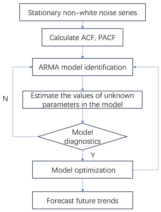
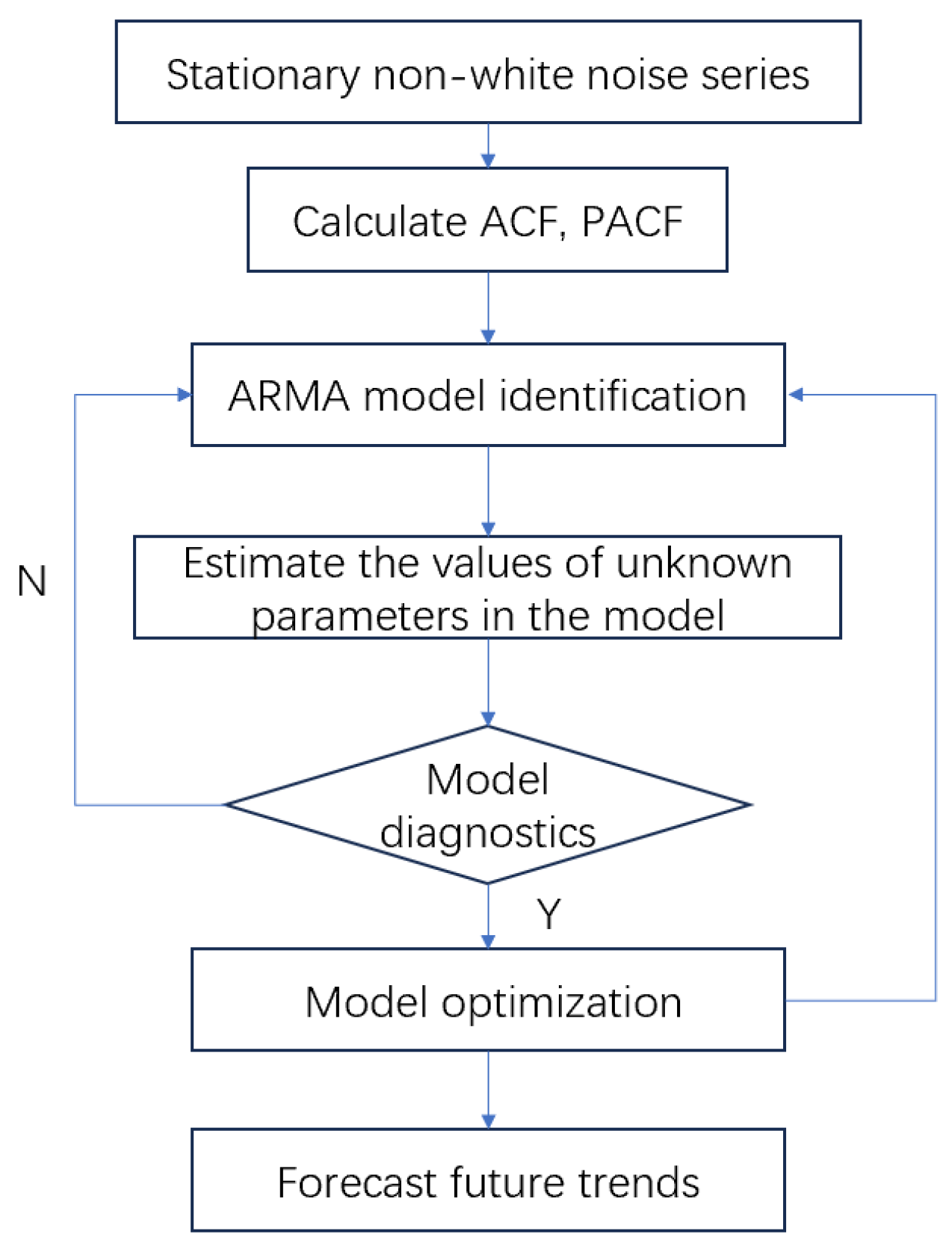
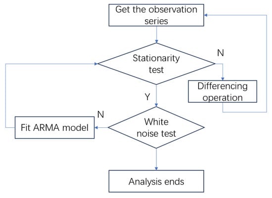
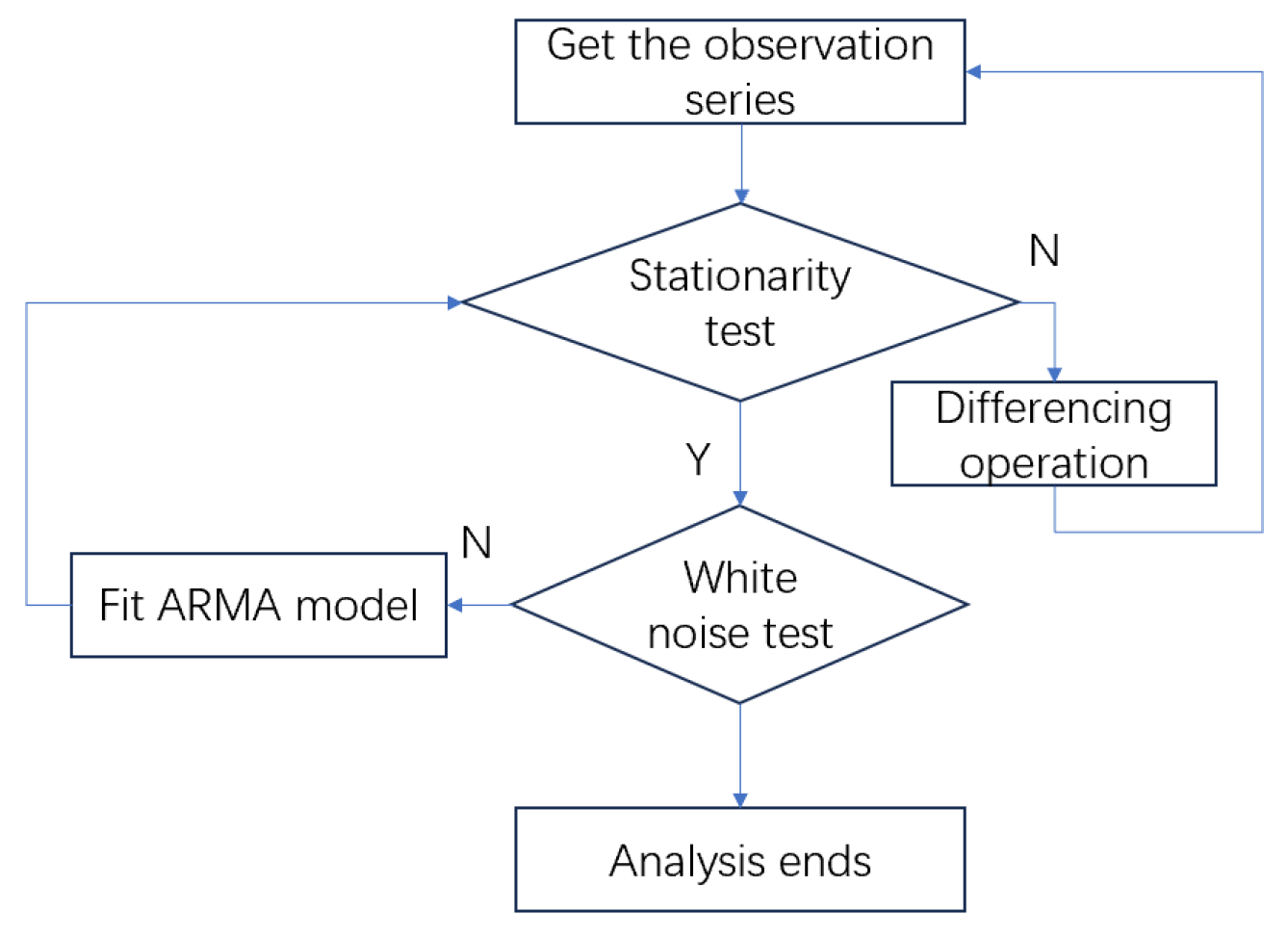
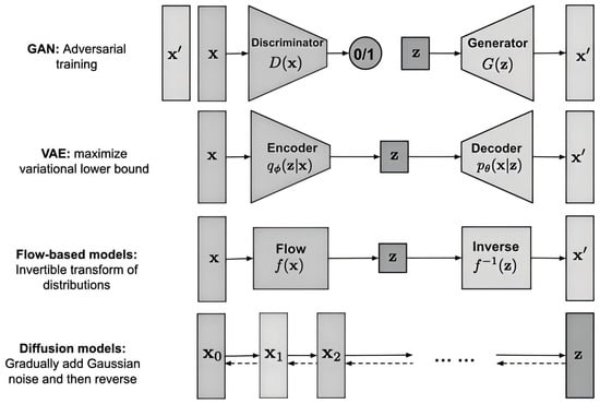
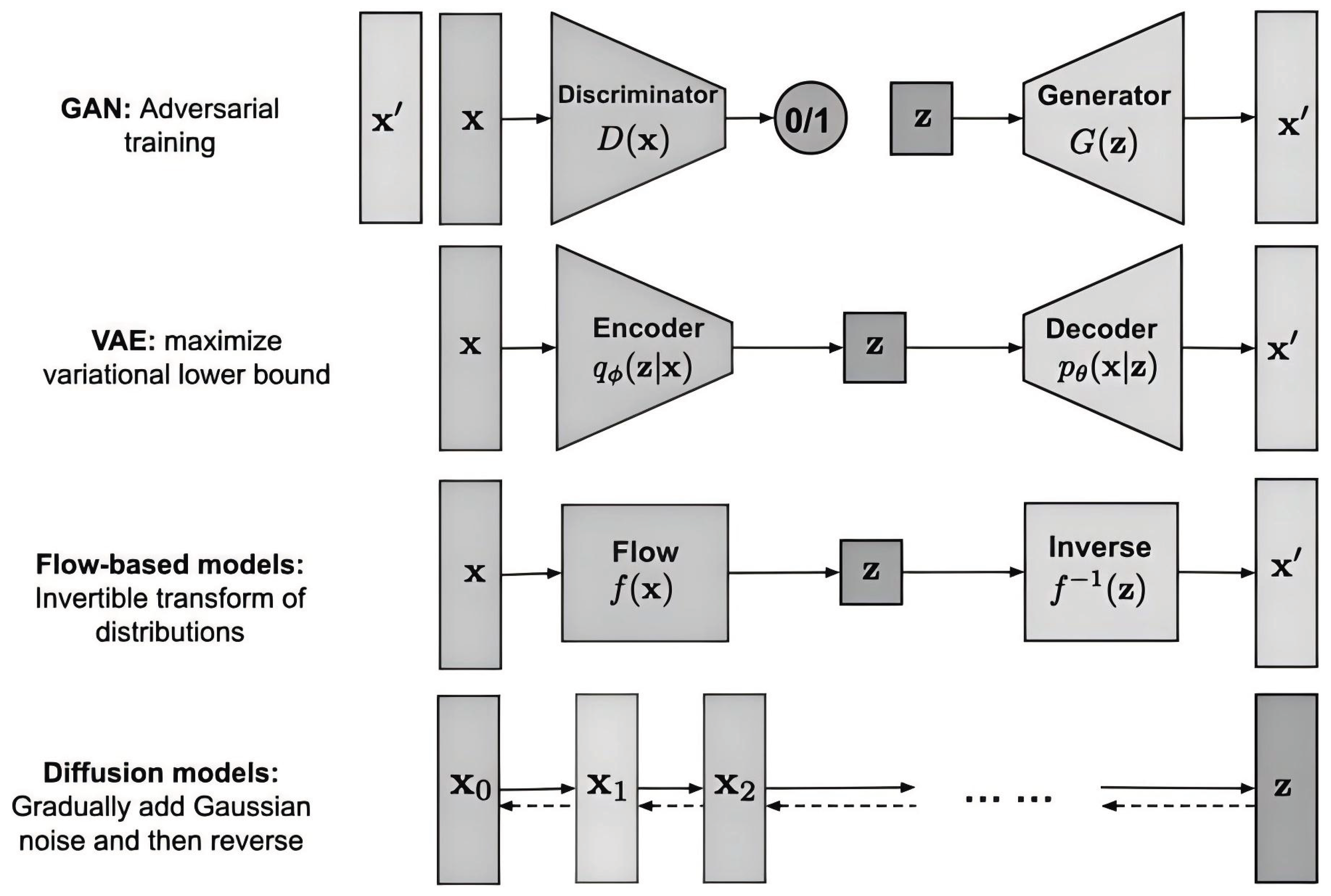
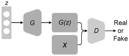
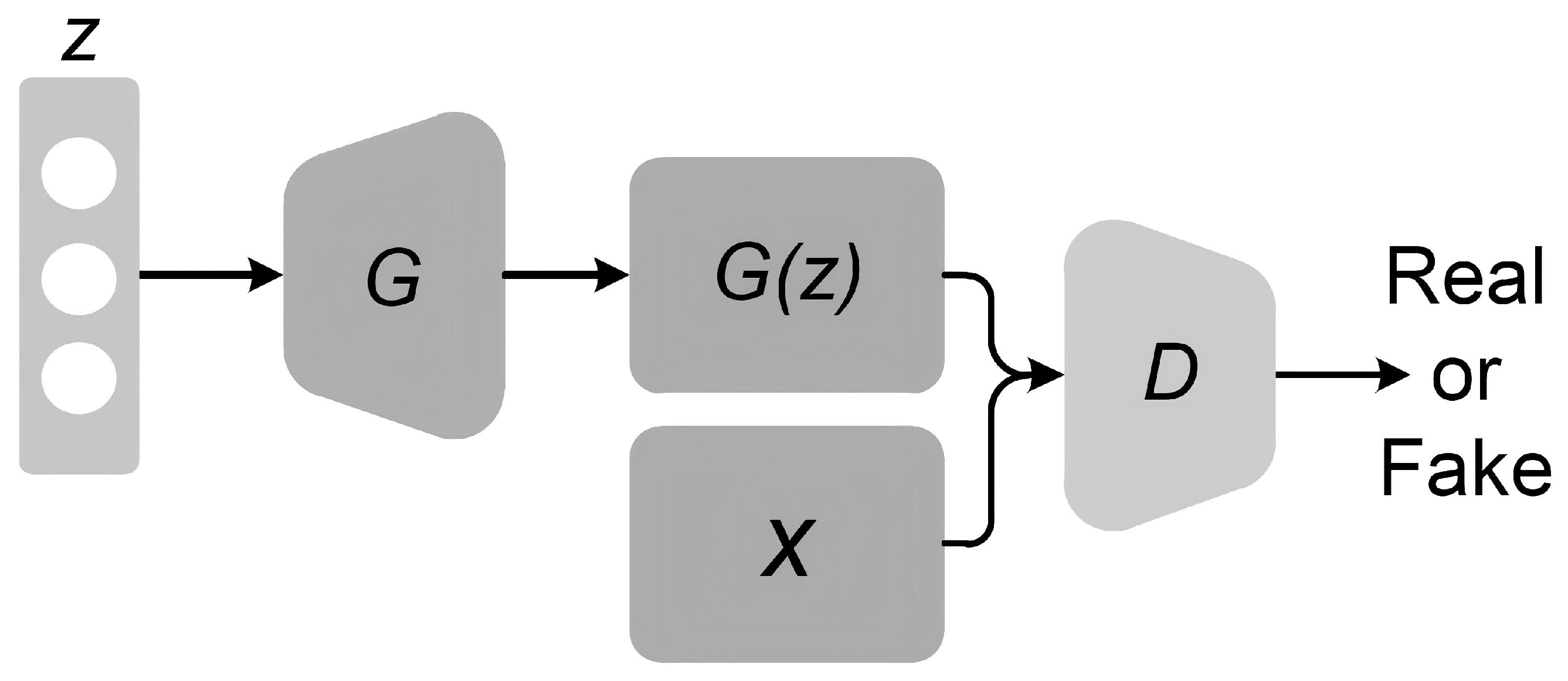
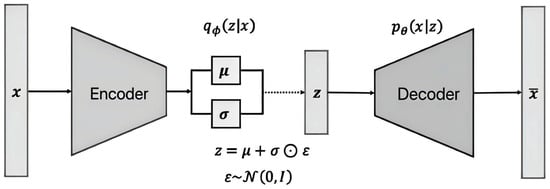
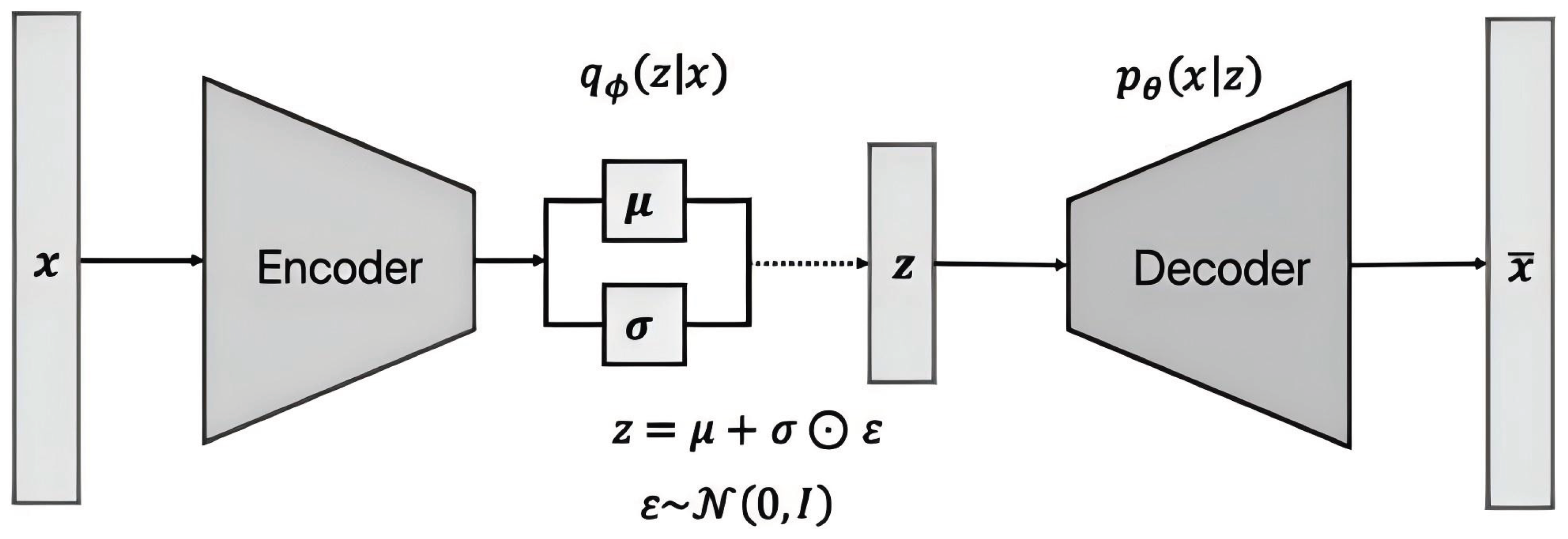
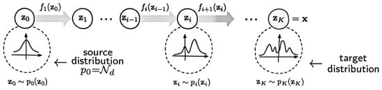
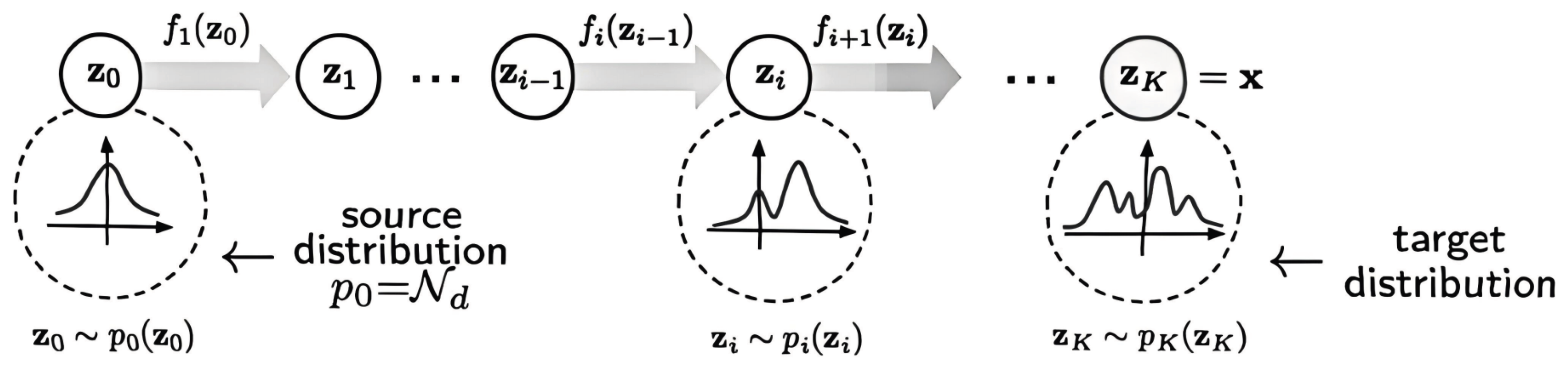
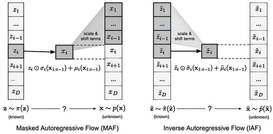
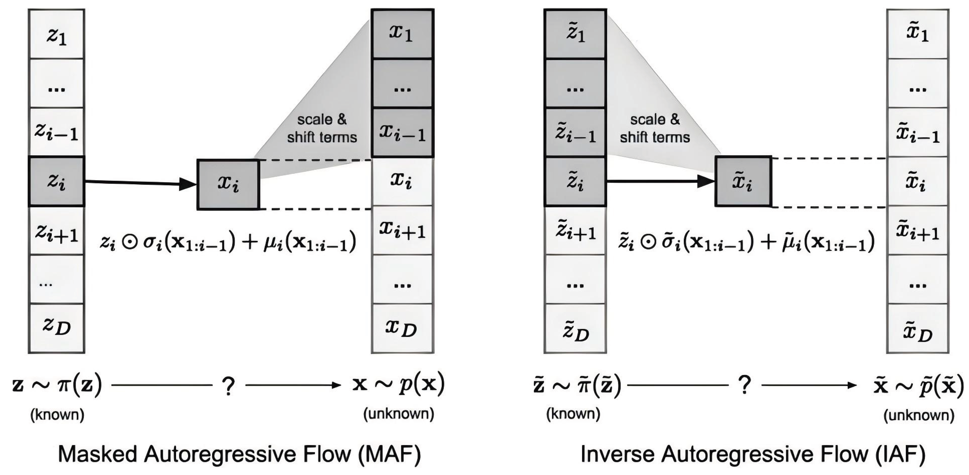
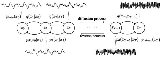
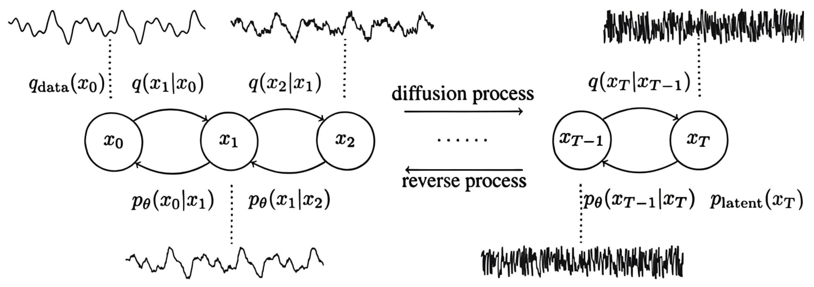

Disclaimer/Publisher’s Note: The statements, opinions and data contained in all publications are solely those of the individual author(s) and contributor(s) and not of MDPI and/or the editor(s). MDPI and/or the editor(s) disclaim responsibility for any injury to people or property resulting from any ideas, methods, instructions or products referred to in the content. |
© 2026 by the authors. Licensee MDPI, Basel, Switzerland. This article is an open access article distributed under the terms and conditions of the Creative Commons Attribution (CC BY) license.