Jump Volatility Forecasting for Crude Oil Futures Based on Complex Network and Hybrid CNN–Transformer Model

Abstract

The crude oil futures market is highly susceptible to policy changes and international relations, which often trigger abrupt jumps in prices. The existing literature rarely considers jump volatility and the underlying impact mechanisms. This study proposes a hybrid forecasting model integrating a convolutional neural network (CNN) and self-attention (Transformer) for high-frequency financial data, based on the complex network characteristics between trading information and multi-market financialization indicators. Empirical results demonstrate that incorporating complex network indicators enhances model performance, with the CNN–Transformer model with a complex network achieving the highest predictive accuracy. Furthermore, we verify the model’s effectiveness and robustness in the WTI crude oil market via Diebold–Mariano tests and external event shock. Notably, this study also extends the analytical framework to jump intensity, thereby providing a more accurate and robust jump forecasting model for risk management and trading strategies in the crude oil futures market.

1. Introduction

The crude oil futures market, which embodies both commodity attributes and financial asset attributes, has exerted profound significance on the global economy and financial systems. Crude oil futures price fluctuations not only directly shape the operational strategies of energy enterprises but also transmit risks to broader financial markets, making their impact indispensable to global economic and financial dynamics. However, the crude oil futures market is highly affected by a range of extreme shocks, such as geopolitical conflicts, extreme weather events, and sudden shifts in global energy demand. These shocks often trigger discontinuous price fluctuations—jump, which typically first emerges in the crude oil futures market before propagating to the spot market. Jumps that serve as a critical input for options not only make the Black–Scholes model [1] and traditional VaR models fail to capture the extreme losses, but cause undermining of the effectiveness of asset allocation and risk management. Therefore, accurately modeling and forecasting jump volatility in crude oil futures prices by incorporating the factor of jumps has long remained a core concern for both market participants and policymakers.

Early research on crude oil futures forecasting primarily focused on conventional econometric models like the Autoregressive Conditional Heteroskedasticity (ARCH) model [2] and the Generalized Autoregressive Conditional Heteroskedasticity (GARCH) model [3]. However, they failed to capture the leptokurtic and heavy-tailed properties empirically observed in crude oil futures return series. With the increasing availability of high-frequency data, the Heterogeneous Autoregressive (HAR) model was proposed by Corsi [4], which incorporates a hierarchical autoregressive structure to better capture volatility’s long memory and heterogeneous characteristics. This seminal work stimulated a wealth of HAR-based extensions, such as those by Andersen et al. [5], Corsi et al. [6], Bollerslev et al. [7], and Patton [8], which further improved predictive performance. Recent studies on crude oil futures forecasting have expanded on traditional econometric models [9,10,11]. But approaches still impose strict distributional assumptions on the models when constructing them; furthermore, the ability to model the complex nonlinear temporal dependencies inherent in high-frequency data remains limited.

With the advancement of computational technologies, machine learning (ML) and deep learning (DL) models have been increasingly applied to financial market forecasting. Ref. [12] demonstrated particular effectiveness in predicting volatility, which exhibits properties of non-stationarity, nonlinearity, clustering, and jump components. Random forest (RF) models have shown promise in handling abrupt jump patterns through kernel functions and feature combinations [12,13]. Ref. [14] provides supervised and unsupervised machine learning techniques on stock market forecasting. However, ref. [13] indicates that the long short-term memory (LSTM) neural network model outperforms machine learning models in forecasting effects. Moreover, refs. [15,16] found that Transformer models exhibit faster model training efficiency and long-term forecasting capability while handling complex multimodal information in financial markets. So far, deep learning has been widely applied in the prediction of financial volatility due to its ability to capture nonlinear dynamic characteristics and long-term dependencies in time series [17,18,19,20,21,22,23].

Although the aforementioned studies can leverage the correlation of time series to predict volatility, they fail to consider the interconnections and interactions between indicators with different attributes. In fact, complex networks can extract the interrelationships between indicators through network structures, thereby further reflecting the complexity of financial networks. For instance, ref. [24] constructed stock volatility networks based on data from the New York Stock Exchange (NYSE) and the National Association of Securities Dealers Automated Quotation (NASDAQ); ref. [25] employed complex networks to investigate risk contagion among financial markets. In addition, other studies have utilized complex networks to analyze the correlations between different financial markets [25,26,27]. While the application of complex networks in financial market research is not uncommon today, there is a scarcity of work exploring the impact of interactions between indicators with different market attributes on crude oil futures price jumps. For the first time, this study adopts complex network indicators to extract the network structures among different financial markets and incorporates them with other information as influencing factors to predict the jump volatility of WTI crude oil futures prices.

This paper aims to develop a hybrid convolutional neural network (CNN)–Transformer volatility prediction model based on topological features of the indicator complex network. First, we construct a highly comprehensive indicator system, covering categories such as market trading information, market sentiment, economic policy uncertainty, geopolitical risk, etc. However, a comprehensive indicator system also inherently gives rise to the inconsistencies in the frequencies of structured data involved. We employ the multivariate imputation by chained equations with random forests (miceforest) to handle data missingness. The XGBoost model is used to rank the importance of indicators, screening out the indicators with higher weights, which are then input into the hybrid convolutional neural network (CNN) and self-attention (Transformer) model for jump prediction. Without considering complex networks, the CNN–attention model achieves the highest prediction accuracy. After introducing the structural features of complex networks, all models show improvements in performance to varying degrees. Additionally, we conducted the Diebold–Mariano (DM) test and impact experiments to verify the accuracy and robustness of the proposed models. The literature review presented in Table 1 offers a summary of revelant studies.

Table 1. Summary table of literature review.

Category	Methods	Market	References
Traditional Econometrics	ARCH, GARCH, HAR, HAR extensions, extended traditional econometric models	Energy Market	[2,3,4,5,6,7,8,9,10,11]
Machine Learning	Random forest (RF), supervised/unsupervised machine learning techniques	Financial Market	[12,13,14]
Deep Learning	LSTM neural network, Transformer, gated recurrent unit (GRU) model, etc.	Financial Market	[13,15,16,17,18,19,20,21,22,23]
Network Structure	Complex networks (stock volatility network construction, risk contagion analysis, inter-market correlation analysis)	Financial Market	[24,25,26,27]

The contributions of this paper are mainly three-fold:

(1)

Indicator System Construction—Construct a multi-dimensional indicator-based complex network system covering market trading information, market sentiment, economic policy uncertainty (EPU), and geopolitical risk (GPR). This system comprehensively encapsulates the potential driving factors of price jumps, overcoming the limitation of incomplete factor coverage in the existing literature.

(2)

Forecast Model Development—Propose a hybrid CNN–Transformer model integrated with complex network topological features. By extracting correlations, cross-market interactions, and core topological features from the indicator network and fusing them with market information, the model leverages the CNN’s strength in capturing local feature associations and the Transformer’s advantage in modeling long-range dependencies to achieve accurate jump volatility prediction.

(3)

Model Comparison and Application—Conduct rigorous validation including one-step/multi-step prediction comparative analysis, Diebold–Mariano (DM) tests, and external event shock experiments. In addition to discussing the predictive advantages of the proposed model compared with other types of models, we also explore the economic relevance of the improved forecasting performance. Finally, the model is extended to the prediction of jump frequency, verifying the practical value of the model in risk management.

This paper is organized as follows: Section 2 introduces the model set-up including calculation of complex network topological characteristics and the jump volatility and CNN–Transformer model for volatility forecasting. Section 3 presents the numerical results of multiple models and the evaluation of volatility forecasting results of the WTI crude oil data. Section 4 outlines a future study on jump intensity. Section 5 presents a discussion. Section 6 provides a conclusion and extension.

2. Theoretical Basis

2.1. Jump Volatility

We model the latent log-price process $Y\left(t\right)$ as a continuous-time Itô semi-martingale process as follows:

$$dY\left(t\right)=\mu \left(t\right)dt+\sigma \left(t\right)dB\left(t\right)+\kappa \left(t\right)dJ\left(t\right),$$

(1)

where $\mu \left(t\right)$ is a continuous drift term with bounded variance, $\sigma \left(t\right)$ is the càdlàg instantaneous volatility, $B\left(t\right)$ is a standard Brownian motion, and $\left(J\left(t\right):t\ge 0\right)$ is a counting point process. The jump size $\kappa \left(t\right)$ is denoted by $\kappa \left(t\right)\equiv Y\left(t\right)-Y(t-)$. Volatility is crucial for asset allocation and risk management. Price fluctuations can be categorized into two types: continuous volatility, primarily reflecting gradual price movements over a period, and jump volatility, which mainly represents large, abrupt price changes occurring over short time intervals in response to unexpected market shocks. A common metric for stock price volatility is the quadratic variation process. The quadratic variation (QV) for the stock price on day t is defined as

$$Q{V}_t={\int }_{t-1}^t{\sigma }^2\left(u\right)du+\sum _{t-1<s\le t}{\left(\Delta Y\left(s\right)\right)}^2,$$

(2)

where ${\int }_{t-1}^t{\sigma }^2\left(u\right)du$ and ${\sum }_{t-1<s\le t}{\left(\Delta Y\left(s\right)\right)}^2$ represent the integrated volatility of the continuous component and the jump component, respectively. The realized volatility (RV) for day t is defined as the sum of squared intraday log-returns: $R{V}_t={\sum }_{s=1}^M{r}_{t,s}^2$, where $r_{t,s}$ denotes the s-th intraday log-return on day t, given by

$$r_{t,s}=Y\left(t-1+{\displaystyle \frac{s}{M}}\right)-Y\left(t-1+{\displaystyle \frac{s-1}{M}}\right),s=1,2,\dots ,M,$$

(3)

where M is the number of price observations sampled during the day. As M approaches infinity, we have the following probability limit:

$$\underset{M\to \infty }{lim}R{V}_t\stackrel{p}{\to }{\int }_{t-1}^t{\sigma }^2\left(u\right)du+\sum _{t-1<s\le t}{\left(\Delta Y\left(s\right)\right)}^2,$$

(4)

Barndorff-Nielsen and Shephard [28] defined the realized bipower variation (BV) as

$$B{V}_t={\displaystyle \frac{\pi }{2}}{\displaystyle \frac{M}{M-1}}\sum _{s=1}^{M-1}\left|r_{t,s+1}\right|\left|r_{t,s}\right|,$$

(5)

and established the following probability limit:

$$\underset{M\to \infty }{lim}B{V}_t\stackrel{p}{\to }{\int }_{t-1}^t{\sigma }^2\left(u\right)du,$$

(6)

therefore, with a sufficiently large number of observations M, Andersen et al. [5] proposed using the difference between realized volatility and bipower variation as an effective estimator of jump variation. To ensure non-negativity, the jump variation is defined as

$$J{V}_t\equiv max[R{V}_t-B{V}_t,0]\stackrel{p}{\to }\sum _{t-1<s\le t}{\kappa }^2\left(s\right).$$

(7)

2.2. Complex Network Topological Characteristics

First, we build a network using our financialization indicators based on Table 2. We then calculate the network’s topological features, which serve as indicators for volatility forecasting. We will first address construction of the financialization indicator pattern network.

Table 2. Predictor variables for jump volatility of crude oil.

Category	Factor Indicators	Frequency
Trading Information	Open Price	Daily
	High Price
	Low Price
	Close Price
	Volume
Market Sentiment	BIAS	Daily
	Moving Average (MA)
	Price Rate of Change (PROC)
	AR
	Buyer Ratio (BR)
	Contrary Operation System (CDP)
	Difference of Moving Averages (DMA)
Financialization	Exchange Rates (USD against EUR, CNY, and major Middle Eastern currencies)	Daily
	CBOE Crude Oil Volatility
	VIX Index
	WTI Crude Oil Futures Price
	S&P 500 Index
Network	Average Degree Centrality	Daily
	Average Shortest Path Length
	Average Network Strength
	Network Closeness Centrality
Economic Policy Uncertainty	Global Economic Policy Uncertainty (GEPU) Index (GDP-weighted average of 21 countries/regions)	Monthly
Geopolitical Risk	Geopolitical Threat Index (GPRT)	Monthly
	Geopolitical Action Index (GPRA)
Energy Information	Oil Production	Yearly
	Oil Consumption

To build this network, we first categorize the daily movement pattern of each financialization indicator into four types—sharp rise, slow rise, sharp decline, and slow decline. The expressions are as follows:

$$\left\{\begin{array}{c}P1:D\ge 0\mathrm{and}CR\ge C{R}^{\prime }(\mathrm{Sharp}\mathrm{Rise})\\ P2:D\ge 0\mathrm{and}CR<C{R}^{\prime }(\mathrm{Slow}\mathrm{Rise})\\ P3:D<0\mathrm{and}CR<C{R}^{\prime }(\mathrm{Sharp}\mathrm{Decline})\\ P4:D<0\mathrm{and}CR\ge C{R}^{\prime }(\mathrm{Slow}\mathrm{Decline})\end{array}\right.$$

(8)

where $C{R}^{\prime }$ (the average 5-day change rate of all indicators) is calculated as

$$C{R}^{\prime }={\displaystyle \frac{1}{N}}\sum _{i=1}^N\overline{C{R}_i}$$

where N is the total number of our financialization indicators, and $\overline{C{R}_i}$ is the 5-day change rate of the i-th indicator (computed via the 5-day sliding window). According to the method above, we construct the symbolic pattern network by using the exchange rates, VIX Index, WTI crude oil futures price, and S&P500 Index.

To extract predictive-relevant features, this study integrates complex network theory with deep learning to forecast stock price trends [29]. We construct directed weighted networks between market information and compute key topological metrics—including Network Average Degree Centrality, Average Network Strength, Network Average Shortest Path Length, and network closeness centrality.

2.2.1. Network Average Degree Centrality

The average degree centrality quantifies the actual connection density of a network, defined as the ratio of actual edges to the maximum possible edges. Higher values of this metric indicate denser inter-node connections in price pattern networks, enhanced node reachability, and increased overall network connection density.

$$P={\displaystyle \frac{1}{N^2}}\sum _{i=1}^N\sum _{j=1}^N{a}_{ij},$$

(9)

where N is the number of nodes in the network and $a_{i,j}$ is the value of the adjacency matrix of the undirected network. If the nodes $i,j$ are connected, then $a_{i,j}$ is 1; otherwise, it is 0.

2.2.2. Average Network Strength

The strength of a network is usually captured by the weights between nodes. The larger the average strength of the network, the fewer the number of nodes in the network, the simpler the composition of the price fluctuation pattern, the smaller the complexity of the network, and the higher the frequency of the same node.

$$S={\displaystyle \frac{1}{N}}\sum _{i=1}^N\sum _{j=1}^N{w}_{ij},$$

(10)

where $w_{ij}$ is the weight of node i to node j, which describes the strength of the connection from node i to node j.

2.2.3. Network Average Shortest Path Length

This measures the degree of separation of the network, and the distance $d_{ij}$ from i to node j is defined as the minimum number of edges required to go from node i to node j. The average shortest path length of the network is all the shortest paths in the network:

$$L={\displaystyle \frac{1}{N(N-1)}}\sum _{i=1}^N\sum _{j=1,j\ne i}^N{d}_{ij}.$$

(11)

The shorter the average shortest path, the fewer intermediate modes are required to switch between stock price modes, which means that modes can be connected by fewer edges and are less affected by other modes, so the overall network conversion efficiency and speed are higher.

2.2.4. Network Closeness Centrality

This can be used to measure the difficulty of information transmission. The closeness of node i to the center can be depicted by the reciprocal of the average shortest path length from other nodes to node i:

$$C_i={\displaystyle \frac{N-1}{{\sum }_{j=1}^N{d}_{ji}}}.$$

(12)

then we can obtain the closeness centrality of the network:

$$C={\displaystyle \frac{1}{N}}\sum _{i=1}^N{\displaystyle \frac{n-1}{N-1}}{\displaystyle \frac{n-1}{{\sum }_{j=1}^{n-1}{l}_{ij}}},(i\ne j),$$

(13)

where $l_{ij}$ is defined as the shortest weighted distance from node i to node j. Elevated network closeness centrality correlates with diminished shortest path distances between nodes, consequently reducing both the frequency of inter-pattern transitions and the duration of transitional phases in price dynamics.

These network properties effectively identify periods of high market volatility and serve as robust volatility forecasting indicators.

2.3. CNN–Transformer Model

Convolutional neural networks (CNNs) are widely used for feature extraction in time series prediction. The main operations of CNNs include convolution and pooling. The convolution operation captures local dependencies by applying a set of filters (convolution kernels) on the input data. The output of the convolution operation can be expressed as

$$\begin{array}{c}{C}_b^l=f\left(\sum C_a^{l-1}\ast W_{ab}^l+B_b^l\right)\\ M{P}_b^l=Maxpooling\left(C_b^l\right)\\ F_b^l=Flatten\left(M{P}_b^l\right)\\ M_b^{l+1}=FC\left(F_a^l·W_{ab}^l+B_b^{l+1}\right),\end{array}$$

(14)

where $C_a^{l-1}$ and $C_b^l$ are the inputs and outputs of the convolutional layer, $W_{ab}^l$ and $B_b^l$ denote the convolutional kernel and bias term of the convolutional layer, respectively, ∗ denotes the convolutional operation, f is the activation function, Maxpooling is the pooling layer, Flatten is the spreading layer, and FC is the fully connected layer.

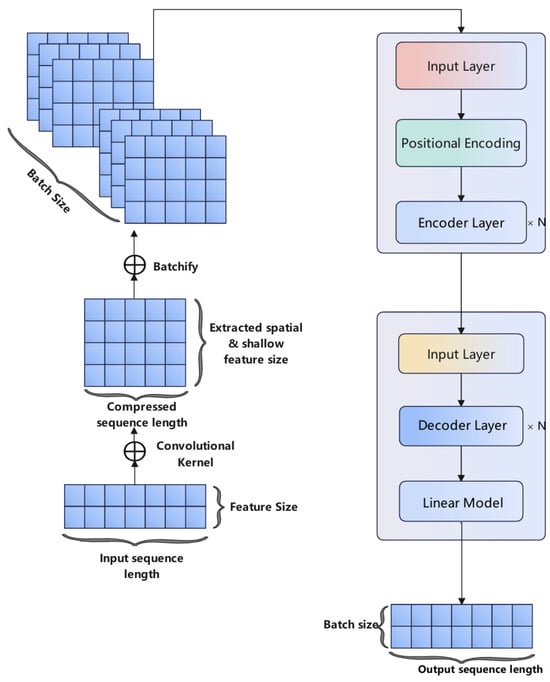
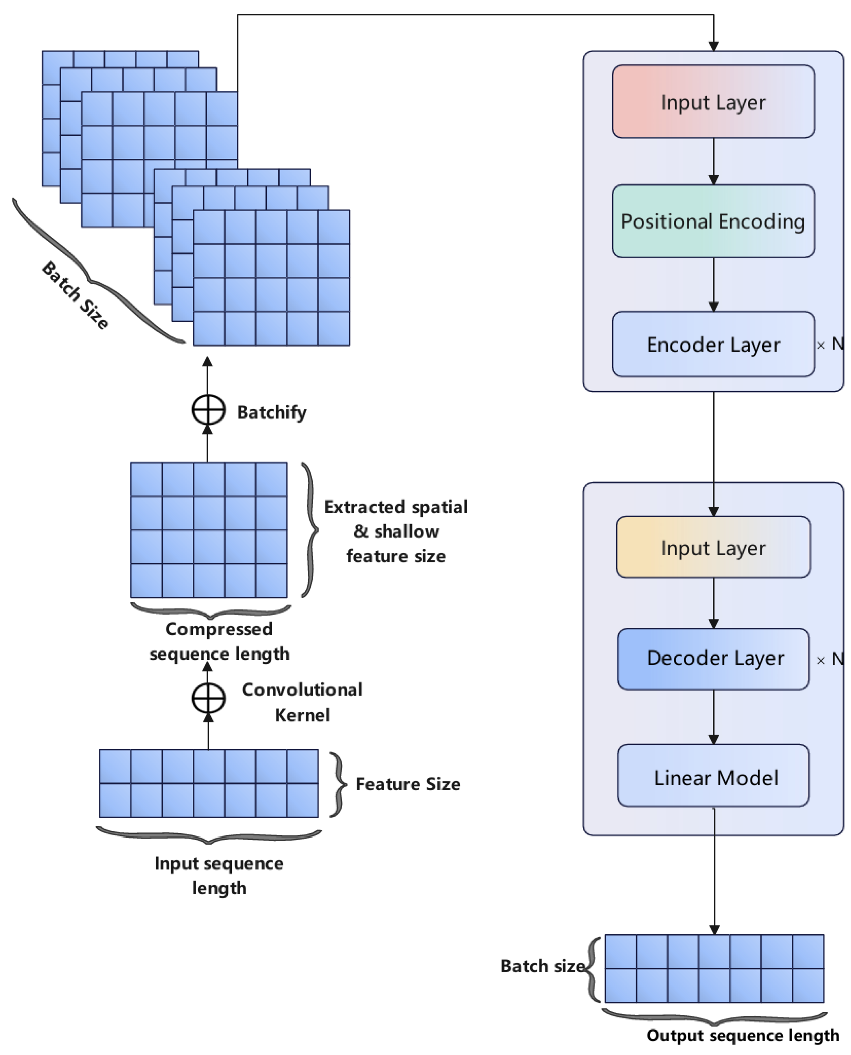
The hybrid CNN–Transformer model combines the strengths of CNN in local feature extraction and Transformer in capturing long-term dependencies. In Figure 1, the structure consists of CNN to extract meaningful features, which are then input into the Transformer model. The CNN component helps capture local patterns, while the Transformer component models global relationships. Traditional RNNs struggle with long sequences due to gradient vanishing/explosion issues. While LSTM and GRU mitigate this through gating mechanisms, the Transformer revolutionizes sequence modeling with its self-attention mechanism. However, since self-attention processes all elements in parallel and lacks inherent sequence awareness, positional encoding is added to the encoder and decoder inputs:

$$\mathrm{input}=\mathrm{input}\mathrm{embedding}+\mathrm{positional}\mathrm{encoding}$$

Figure 1. CNN–Transformer structure.

(1)

Self-Attention Mechanism

The mechanism first generates three vectors (Query, Key, Value) via linear transformations:

$$Q=X{W}^Q,K=X{W}^K,V=X{W}^V,$$

where $W^Q,W^K,W^V$ are trainable parameter matrices. The input X is projected into these vectors to enhance model flexibility. The Query vector represents the relevance of other tokens to the current one, the Key vector stores retrievable information, and the Value vector holds the actual content.

The attention scores are computed as

$$A=softmax\left({\displaystyle \frac{Q{K}^T}{\sqrt{d_k}}}\right)V,$$

where $d_k$ is the dimension of K. The scaling factor ($\sqrt{d_k}$) stabilizes gradients by preventing large variances in $Q{K}^T$. The softmax normalizes scores into weights (0–1) per row.

To further boost performance, Multi-Head Attention employs multiple sets of $W^Q,W^K,W^V$:

$${head}_i=\mathrm{Attention}\left(X{W}_i^Q,X{W}_i^K,X{W}_i^V\right),$$

(2)

Add and Norm

To mitigate gradient vanishing during backpropagation, each encoder/decoder layer uses residual connections and layer normalization:

$$\mathrm{LayerNorm}(x+\mathrm{Sublayer}(x\left)\right)$$

this structure enhances information flow and training efficiency.

(3)

Feed-Forward Neural Network (FFNN)

The FFNN captures nonlinear patterns via two fully connected layers:

$$FFN\left(x\right)=ReLU\left(x{W}_1+b_1\right)W_2+b_2,$$

For the task of predicting jump volatility in this research, the input sequence $X\in {\mathit{R}}^{n\times d}$ is composed of n historical time steps with d-dimensional features. These features are first transformed into d-dimensional embeddings via linear projection, then processed through N stacked encoder layers to extract multi-scale temporal patterns, and finally passed through a fully connected layer to generate predictions for T future time steps.

2.4. Bayesian Optimization Procedure

Bayesian optimization is an efficient black-box optimization algorithm, primarily used to find the optimal parameter combination in the hyperparameter space. It is suitable for scenarios with high hyperparameter dimensions and high model training costs. Compared with grid search (which iterates through all combinations) and random search (which performs undirected random sampling), Bayesian optimization can find a better hyperparameter combination with fewer iterations, significantly saving computational resources.

(1)

Define the objective function and hyperparameter space: Minimize the RMSE of jump volatility (JV) predictions on the validation set; define the hyperparameters to be optimized for CNN, Transformer, and XGBoost along with their ranges.

(2)

Surrogate model: Since the objective function is a black box with high evaluation costs, Bayesian optimization first constructs an inexpensive probabilistic surrogate model to fit the mapping relationship between the hyperparameter combination and objective function. In this study, we select a Gaussian process as the surrogate model.

(3)

Define the acquisition function: Based on the prediction results of the surrogate model, screen the next most worthy hyperparameter combination to balance “Exploration” and “Exploitation”. Exploitation refers to prioritizing hyperparameters predicted by the surrogate model to obtain the optimal(local optimum) objective function value. Exploration refers to prioritizing hyperparameters with high uncertainty predicted by the surrogate model. In this study, we use Expected Improvement (EI) as the acquisition function.

(4)

Evaluate the objective function value: Construct the corresponding model (e.g., LSTM, CNN, Transformer) using the “optimal candidate hyperparameter combination” selected by the acquisition function. Train the model on the training set and evaluate its performance on the validation set to obtain the objective function value (RMSE).

(5)

Number of iterations: Repeat steps 3 and 4 for iteration until the change in RMSE is less than the threshold.

(6)

Output: After the iteration stops, select the hyperparameter combination with the optimal objective function value (i.e., the minimum RMSE on the validation set) from all evaluated combinations as the final model’s hyperparameter configuration, which is used for subsequent test set validation and practical prediction.

2.5. Evaluation Criteria

To comprehensively evaluate the predictive accuracy, this study establishes a multi-faceted assessment framework by employing six distinct loss functions to quantify forecast performance across methodologies. Specifically, the error distributions of all models were subjected to rigorous comparative analysis using the following metrics: Root Mean Square Error (RMSE), Mean Absolute Error (MAE), Symmetric Mean Absolute Percentage Error (SMAPE), Mean Squared Logarithmic Error (MSLE), Mean Bias Error (MBE), and standard deviation (SD). The formal definitions of these evaluation criteria are articulated as follows:

$$\begin{array}{cc}\hfill & \begin{array}{c}\mathrm{RMSE}=\sqrt{{\displaystyle \frac{1}{N}\sum _{n=1}^N}{\left({\widehat{y}}_n-y_n\right)}^2},\\ \mathrm{MAE}={\displaystyle \frac{1}{N}}{\displaystyle \sum _{n=1}^N}\left|{\widehat{y}}_n-y_n\right|,\\ \mathrm{SMAPE}={\displaystyle \frac{1}{N}}{\displaystyle \sum _{n=1}^N}{\displaystyle \frac{\left|{\widehat{y}}_n-y_n\right|}{\left(\left|{\widehat{y}}_n\right|+\left|y_n\right|\right)/2}},\\ \mathrm{MSLE}={\displaystyle \frac{1}{n}}\sum {\left(ln(1+Y)-ln\left(1+Y_F\right)\right)}^2,\\ \mathrm{MBE}={\displaystyle \frac{1}{N}}{\displaystyle \sum _{n=1}^N}\left({\widehat{y}}_n-y_n\right),\\ \mathrm{SD}=\sqrt{{\displaystyle \frac{{\sum }_{n=1}^N{\left({\widehat{y}}_n-\mathrm{Arithmetic}\mathrm{mean}\right)}^2}{\mathrm{total}\mathrm{number}}}},\end{array}\hfill \end{array}$$

(15)

where $y_n$ indicates the true value and ${\widehat{y}}_n$ indicates the predicted value.

DM Test

The Diebold–Mariano (DM) [30] test is the statistical method for testing the significance of predictive accuracy differences. In empirical applications, it is often the case that two or more time series models are available for forecasting a particular variable of interest.

$$\begin{array}{cc}\hfill \mathrm{Actual}\mathrm{values}\text{:}& \left\{y_n;n=1,\dots ,N\right\}\hfill \\ \hfill \mathrm{Two}\mathrm{forecasts}\text{:}& \left\{{\widehat{y}}_{1n};n=1,\dots ,N\right\},\left\{{\widehat{y}}_{2n};n=1,\dots ,N\right\}.\hfill \end{array}$$

(16)

Define the forecast errors as

$$e_{in}={\widehat{y}}_{in}-y_n,i=1,2$$

the loss associated with forecast i is assumed to be a function of the forecast error, $e_{it}$, and is denoted by $g\left(e_{in}\right)$. The function $g(.)$ is a loss function. Typically, $g\left(e_{in}\right)$ could be the square (squared error loss) or the absolute value (absolute error loss) of $e_{in}$. In this study, we adopt MSE as the loss function.

We define the loss differential between the two forecasts by

$$d_n=g\left(e_{1n}\right)-g\left(e_{2n}\right)$$

and DM statistics can be calculated as follows:

$$DM={\displaystyle \frac{\overline{d}}{\sqrt{\frac{{\sum }_{n=1}^N{\left(d_n-\overline{D}\right)}^2}{T-1}}}}\to N(0,1)$$

where $\overline{d}={\sum }_{n=1}^N{d}_n$ is the sample mean of the loss differential. Say that the two forecasts have equal accuracy if and only if the loss differential has zero expectation for all t. So, we would like to test the null hypothesis

$$H_0:E\left(d_n\right)=0;$$

versus the alternative hypothesis

$$H_1:E\left(d_n\right)\ne 0$$

the null hypothesis is that the two forecasts have the same accuracy. The alternative hypothesis is that the two forecasts have different levels of accuracy.

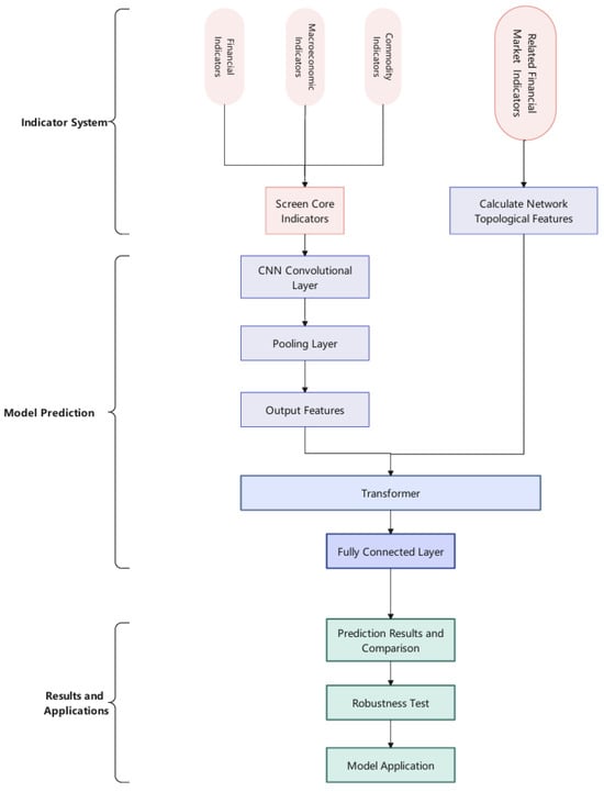
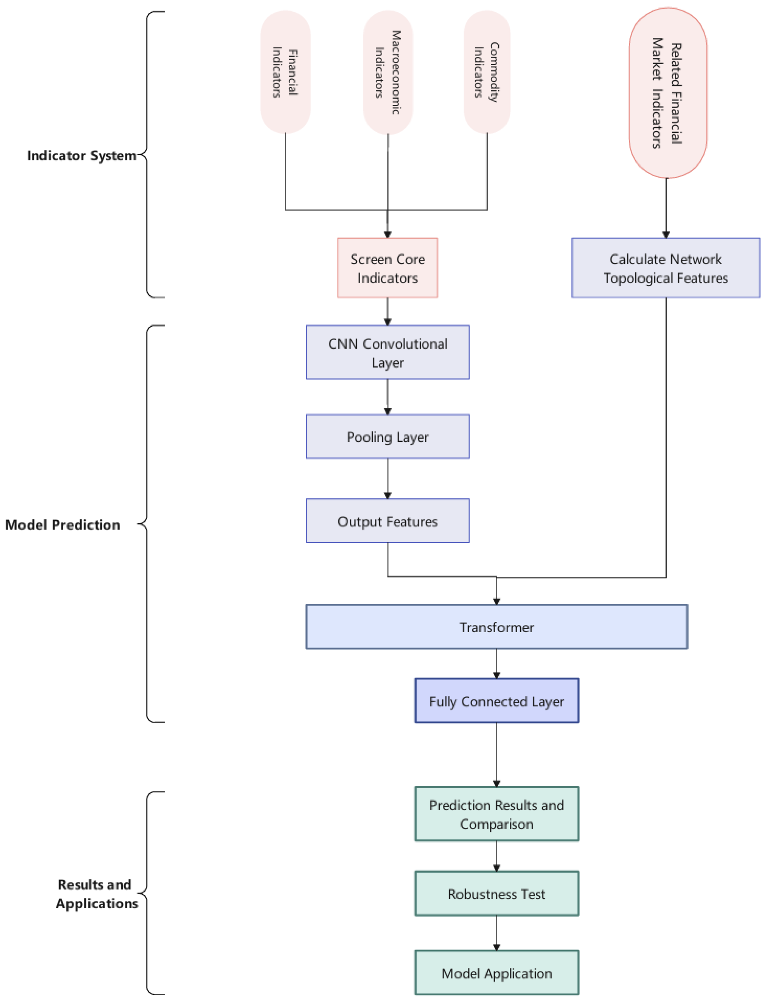
Figure 2 illustrates the workflow for jump volatility forecasting. This research framework consists of three core modules: indicator system construction, model development, and result comparison and application. Financial indicators are categorized into three types, and network topological features are calculated based on financialization indicators. In the model prediction module, the selected core indicators are first processed by CNN convolutional layers and pooling layers to extract local features. After fusing these output features with network topological features, the combined features are input into the Transformer to capture long-range dependencies in the data. Finally, prediction results are generated via the fully connected layer.

Figure 2. The workflow of jump volatility forecasting.

3. Numerical Results

3.1. Data Sources and Variables

Research on oil prices not only serves as a core topic in energy economics but also plays a pivotal role in global economic functioning, the operation of financial markets, and the formulation of investment decisions. As one of the three major global crude oil pricing benchmarks alongside Brent and Dubai crude oil benchmarks, West Texas Intermediate (WTI) exhibits price fluctuations that exert a profound impact on the core operations of energy-dependent economies. Characterized by a high level of financialization and heightened geopolitical sensitivity, the WTI market further exhibits distinct jump dynamics, which are critical for understanding its price behavior.

For the empirical analysis, this study employs West Texas Intermediate (WTI) crude oil futures price data covering the period from 4 January 2010 to 8 April 2024, encompassing 3655 consecutive trading days. To mitigate the impact of market microstructure noise while retaining critical volatility dynamics, a systematic 5 min interval sampling method is adopted, resulting in exactly 48 discrete price observations per trading day. The training set in this study is constructed using data from 2010 to 2018, and the test set is restricted to data covering the subsequent period between 2019 and 2024.

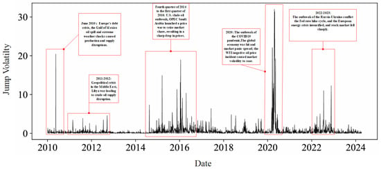
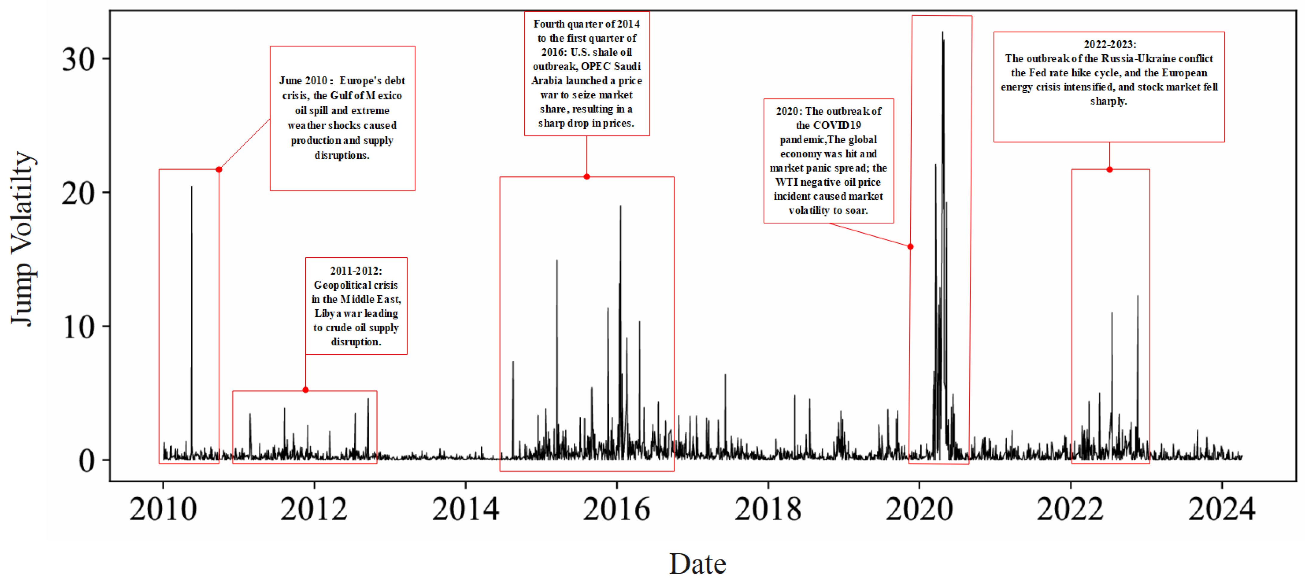
Figure 3 presents the jump volatility of WTI, which maps external event shocks to the time periods during which JV exhibited sharp fluctuations. In general, sharp fluctuations in jump volatility are typically attributable to a range of external event shocks, including wars, government policy adjustments, geopolitical conflicts, and epidemic-related disruptions. Specifically, in 2011–2012, the Libyan Civil War disrupted crude oil supplies; combined with supply-side panic induced by Western sanctions, WTI prices surged, and the Oil Volatility Index (OVX) exceeded 50%. In 2015, the price war initiated by Saudi Arabia within the Organization of the Petroleum Exporting Countries (OPEC) led to a 75% plunge in WTI prices. From 2020 to 2022, the global crude oil market experienced substantial fluctuations, driven by the severe impacts of multiple factors: the outbreak of the COVID-19 pandemic, the Russia–Ukraine conflict, and escalating geopolitical tensions.

Figure 3. Jump volatility of WTI from 2010 to 2024.

Feature selection stands as a pivotal determinant of model performance in financial forecasting. In high-frequency financial market analysis, trading information indicators and market indicators have long been recognized as core predictors for short-term market behaviors, a practice widely validated by the existing literature [31,32,33]. However, recent studies have increasingly highlighted that macroeconomic factors also exert non-negligible impacts on extreme market events like price jumps. For instance, ref. [34] pointed out that international financial crises could amplify and propagate the impacts of uncertainty shocks. Ref. [35] specifically explored the shock transmission mechanism and volatility responses under policy uncertainty. Meanwhile, macro variables (e.g., monthly Global Economic Policy Uncertainty (GEPU) and geopolitical risk (GPR)) exert more immediate influences [10,36,37]. These mechanisms collectively illustrate that macroeconomic variables are not merely external contextual factors; they serve as core drivers of jump volatility, acting as a bridge for risk transmission between the macroeconomy and financial markets. In summary, the indicator system of this study integrates high-frequency trading indicators and critical macro variables, forming a comprehensive framework that captures both short-term trading dynamics and long-term risk transmission paths. The specific indicators are presented in Table 2.

Regarding the data sources of the predictor variables for crude oil jump volatility categorized in the table, the specific details are elaborated as follows: The data for all indicators categories are retrieved from https://www.wind.com.cn (accessed on 9 April 2024). For the Financialization category, the relevant factor indicators are sourced from https://cn.investing.com (accessed on 9 April 2024). The Global Economic Policy Uncertainty (GEPU) Index under the “Economic Policy Uncertainty” category is obtained from http://www.policyuncertainty.com (accessed on 9 April 2024). The Geopolitical Threat Index (GPRT) and Geopolitical Action Index (GPRA) in the Geopolitical Risk category are derived from https://www.matteoiacoviello.com (accessed on 9 April 2024). Finally, the oil production and consumption data are collected from https://www.eia.gov/international/overview/world (accessed on 9 April 2024), and the details of Market Sentiment indicators calculation are persented in Appendix A.

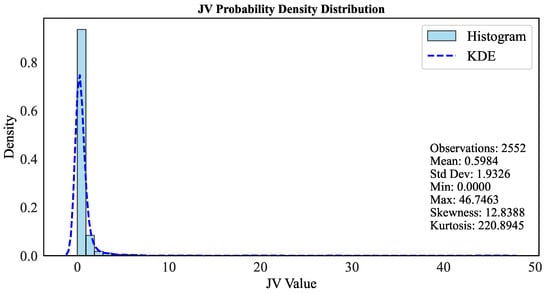
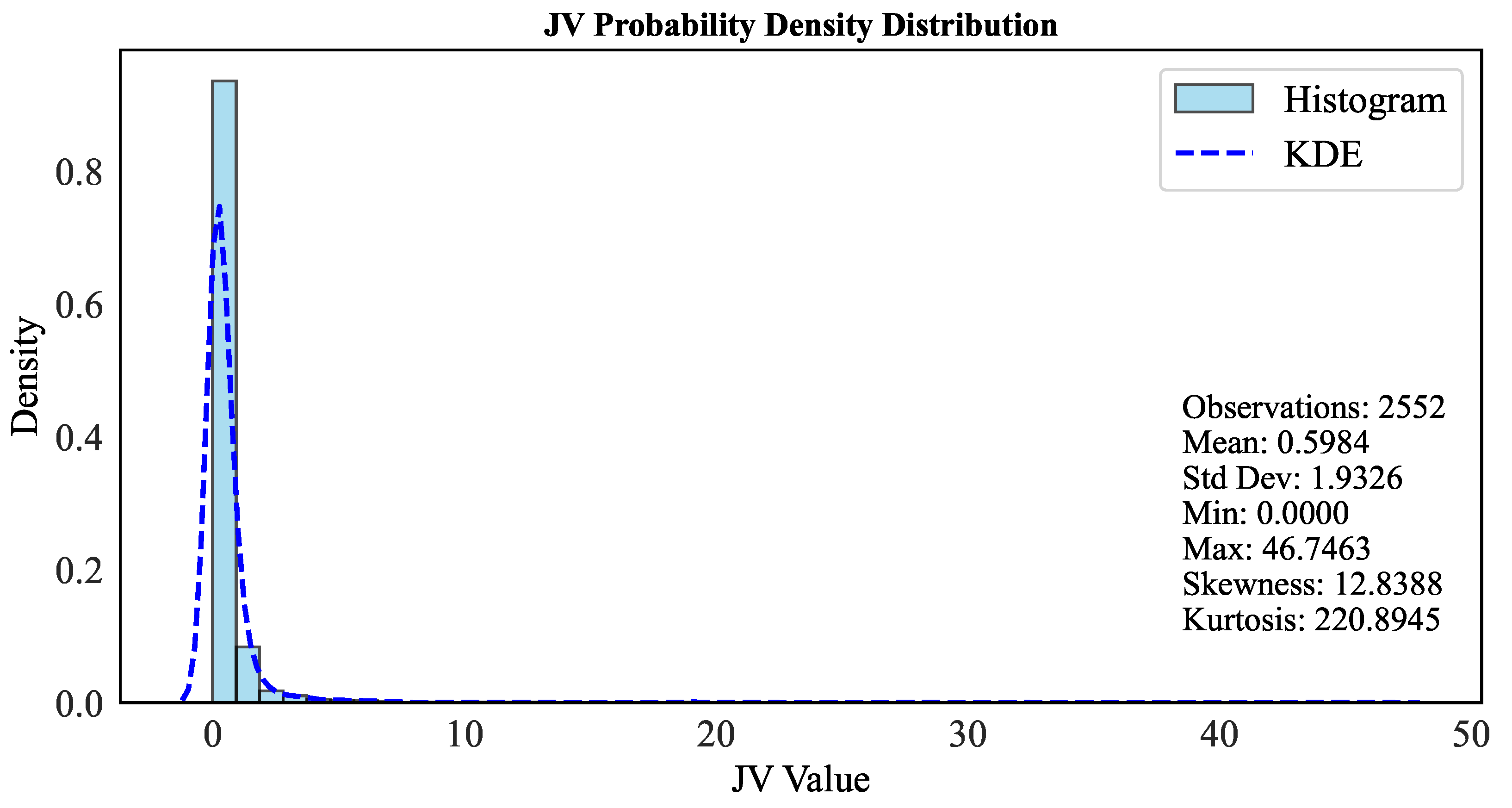
Table 3 presents the descriptive statistics of all indicators, along with the Probability Density Distribution (PDF) of jump volatility (JV). Taking JV as an example, its mean is 0.5984, paired with a standard deviation of 1.9326, which indicates considerable volatility. The minimum value of JV is 0 while the maximum reaches 46.7463, reflecting substantial discrepancies between typical and extreme jump levels.

Table 3. Descriptive statistics of indicators.

Indicator	Mean	Std	Min	Max	Skew	Kurtosis
JV	0.5984	1.9326	0.0000	46.7463	12.8388	220.8945
Close	71.6834	21.8262	12.3400	123.7000	−0.0398	−0.9915
Open	71.7138	21.8584	12.9600	124.6600	−0.0357	−0.9877
High	72.7721	21.9952	13.6900	130.5000	−0.0177	−0.9973
Low	70.5566	21.6291	10.0700	120.7900	−0.0538	−0.9753
Volume	$3.9092\times {10}^5$	$2.1869\times {10}^5$	1980.0000	$1.7700\times {10}^6$	0.8473	1.1881
PROC	0.0010	0.0474	−0.3533	0.2851	−0.2067	7.0791
MA	71.6219	21.8717	4.1860	120.9260	−0.0493	−0.9799
BIAS	0.0044	0.1129	−0.2686	4.0000	26.9441	832.4133
AR	97.3183	29.2445	36.5069	372.0588	1.2493	5.8275
BR	0.9638	0.2967	0.1489	2.2208	0.9464	0.6862
CDP	71.6739	21.8104	12.1100	123.4775	−0.0391	−0.9942
DMA	0.0037	1.3890	−8.5940	10.1420	−0.2053	4.6822
Kuwait	0.2963	0.0109	0.2718	0.3108	−0.7025	−1.0846
Iran	$3.0366\times {10}^4$	$1.2288\times {10}^4$	9834.0000	$4.4120\times {10}^4$	−0.5739	−1.1914
Europe	1.1948	0.1140	0.9594	1.4826	0.4913	−0.8766
RMB	6.5899	0.3175	6.0930	7.2472	0.1614	−1.1431
VIX	18.4918	7.1454	9.1500	82.6900	2.4884	12.0575
Futures	71.6014	21.5640	17.6000	119.7800	−0.0240	−1.0567
OVX	37.6314	16.8166	14.6700	236.8000	4.6342	36.0839
SP500	257.8204	110.4516	102.7600	523.1700	0.5237	−0.8766
P	0.0653	0.0169	0.0000	0.1700	1.5075	4.6341
L	3.8257	1.2480	0.0000	10.0316	1.5780	3.4077
S	1.1708	0.1342	0.0000	2.0000	0.9884	5.1181
C	0.1183	0.0385	0.0000	0.2805	0.7551	0.5189
GPR	103.9159	30.7643	58.4200	318.9500	1.0785	2.3024
GPRT	113.7354	38.8437	59.0200	403.7100	1.7081	6.9957
GPRA	95.9653	40.9476	28.4500	250.9600	1.0783	0.7263
GEPU_current	191.6519	65.0726	86.5941	431.5421	0.6509	−0.1418
GEPU_ppp	196.8268	67.7209	85.7250	436.6362	0.5460	−0.5142
Production	$9.5801\times {10}^4$	4255.8813	$8.7384\times {10}^4$	$1.0281\times {10}^5$	−0.3452	−0.7567
Consumption	$9.5497\times {10}^4$	4079.4312	$8.8831\times {10}^4$	$1.0186\times {10}^5$	−0.2001	−1.3772

Figure 4 depicts the histogram and Kernel Density Estimation (KDE) of JV. It can be observed that JV values are predominantly concentrated around 0, implying that most periods exhibit low jump volatility. The long right tail of the distribution corresponds to the positive skewness and high kurtosis of JV (as presented in Table 3), which confirms that extreme high-jump events—though infrequent—do occur in practice.

Figure 4. JV Probability Density Distribution.

To select optimal hyperparameters (e.g., kernel size, dropout rate, and learning rate) for the CNN, Transformer, and LSTM models, we employ Bayesian optimization. Hyperparameters are selected iteratively via Bayesian optimization: based on the Gaussian process surrogate model to predict the performance distribution of hyperparameter combinations, the Expected Improvement (EI) acquisition function is used to balance exploration and exploitation, gradually converging to the optimal hyperparameter combination that minimizes the mean squared error (MSE) of volatility prediction. The parameters of the CNN, Transformer, and LSTM models selected via Bayesian optimization are presented in Table 4.

Table 4. The optimal values for hyperparameters in CNN, Transformer, and LSTM models selected through Bayesian optimization.

Model	Hyperparameter	Value
CNN	activation	tanh
	kernel_size	3
	strides	1
	dropout_rate	0.2
Transformer	num_blocks	2
	embed_dim	64
	dense_dim	32
	num_heads	2
	dropout_rate	0.1
	learning_rate	0.1
	activation	tanh
LSTM	unit1	32
	unit2	64
	activation	tanh
	dropout_rate	0.2
	batch_size	16
	learning_rate	0.005

Since XGBoost can effectively capture the nonlinear correlations among financialization indicators and quantify feature importance, we adopt XGBoost for variable selection. The specific process of variable selection using XGBoost in this study is as follows: First, preprocess financialization indicators (including cross-country exchange rates, OVX, WTI crude oil futures, S&P500 Index, and their derived features) to construct a full-variable dataset—this involves handling missing values, correcting outliers, standardizing dimensions (Z-score normalization), and partitioning data into training, validation, and test sets in chronological order (to avoid data leakage in time series). Second, train an XGBoost model using the full-variable dataset and calculate feature importance with Gain as the core metric. Gain quantifies the total reduction in the loss function (mean squared error, MSE) contributed by each variable across all decision trees, directly reflecting the variable’s explanatory power for jump volatility prediction. Third, screen core variables based on Gain values and stepwise screening. Finally, reconstruct the XGBoost model using the screened core variables and confirm it as the final model for prediction—this ensures that the model is both parsimonious and predictive, laying a foundation for subsequent integration with the CNN–Transformer framework.

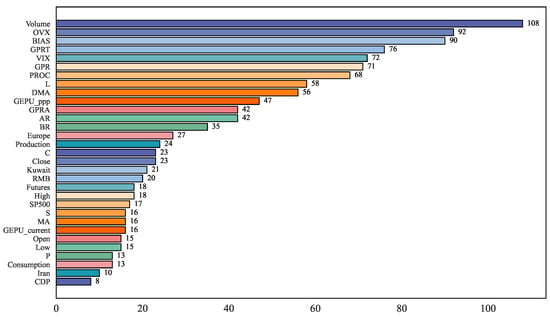
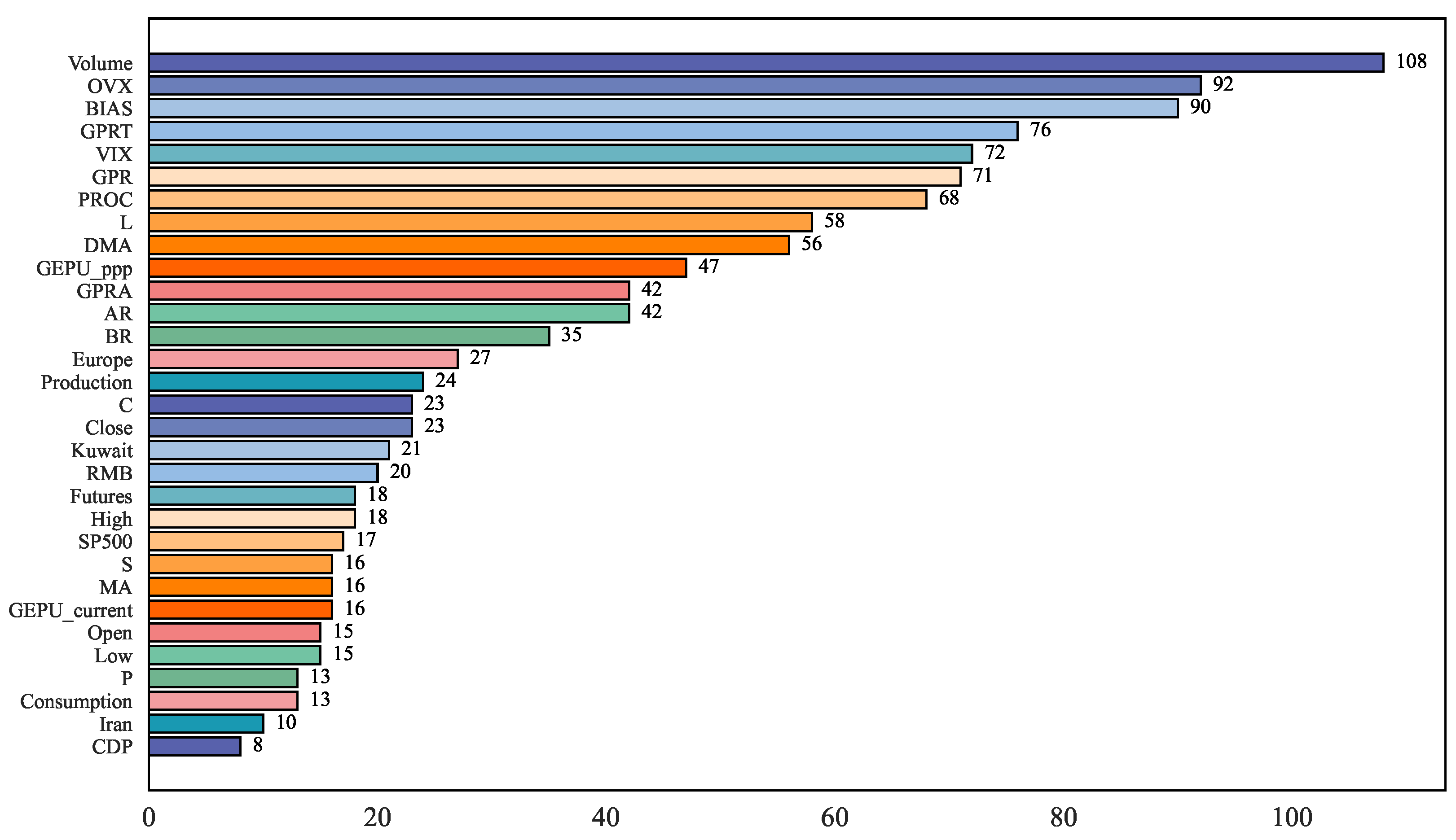
Figure 5 presents the feature importance ranking based on the XGBoost model. Volume, OVX (CBOE Crude Oil ETF Volatility Index), and BIAS play core roles in model prediction, which indicates that they are closely related to market jump and the switching of price trends, serving as key signals for changes in market operation. In addition, due to the association with macro-environmental shocks and regional factors, geopolitical risk ranks among the top ten in terms of importance, reflecting that the model has the ability to capture the regional economic and political dynamics of various countries. Moreover, other related features (such as VIX, network, etc.) are also concentrated in the high-importance interval, strongly highlighting the supporting value of the internal correlation of financial data for prediction work.

Figure 5. The importance of features based on XGBoost.

3.2. Data Preprocessing

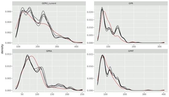
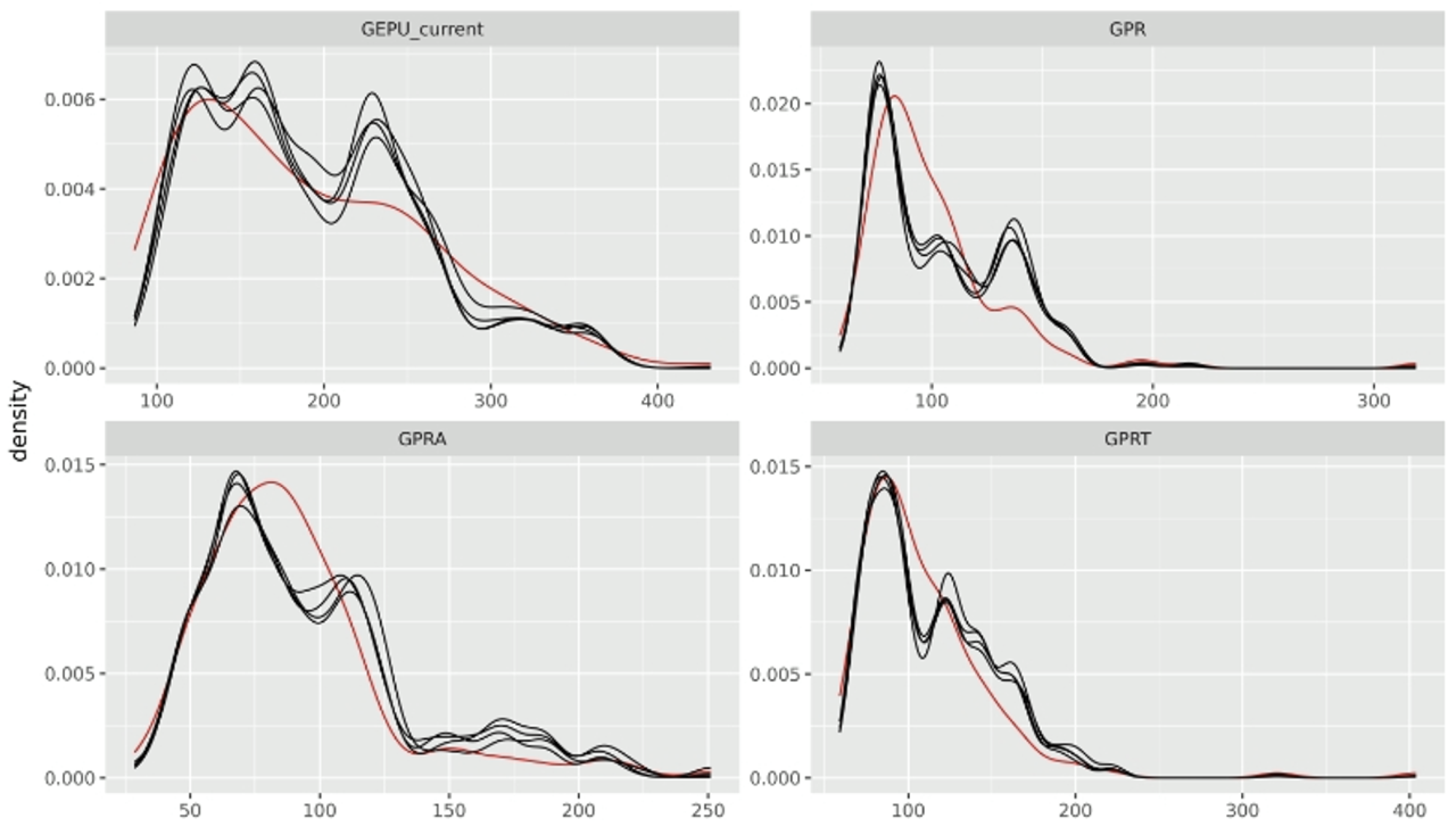
After calculating the feature sets of liquidity and technical indicators, the data needs to be normalized because the features are on different scales. To address this limitation, our study adopts a random forest-based Chained Equations Multiple Imputation method (MICEForest) [38] to harmonize all variables into daily frequency and effectively impute long-period missing values. Figure 6 presents the imputation distribution of the four monthly indicators of WTI. The x-axis represents the values of each variable (GEPU, GPR, GPRA, GPRT), and the y-axis denotes the density function of the corresponding data distribution. The red line represents the original data, while each black line indicates the value of the imputed data from each iteration in each dataset. As evident from the figure, the interpolation method demonstrates good consistency with the distribution of the original data, which in turn minimizes unintended perturbations to the original dataset, thereby validating its ability to preserve the intrinsic properties of the raw data.

Figure 6. Data imputation distribution.

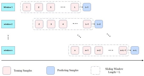
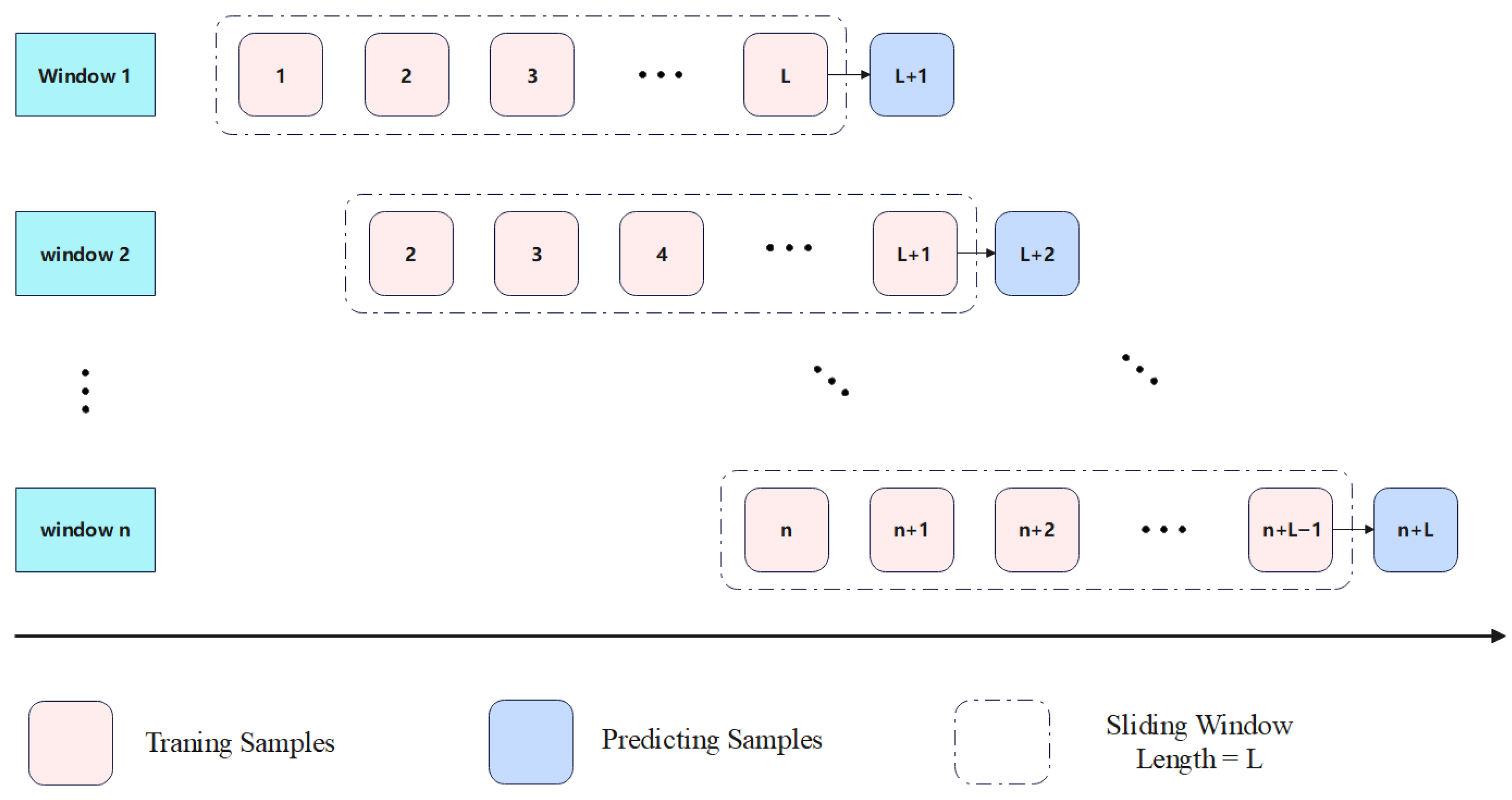
In order to capture new trends and patterns in the data in time, this paper uses a sliding time window for rolling prediction according to [39], and predicts jump volatility of the next day by rolling the historical data of the past L days, as shown in Figure 7. In order to analyze the influence of training step size on the prediction effect of the CNN–Transformer model, this paper selects training step sizes of 10, 20, 30, and 40 days to construct training data, and the corresponding prediction results are shown in Table 5.

Figure 7. Schematic diagram of rolling prediction.

Table 5. CNN–Transformer prediction under different lengths.

History Length	RMSE	MAE	SMAPE	MSLE	MBE	SD
10	0.8460	0.6810	0.5120	0.1300	−0.4650	0.2710
20	0.9100	0.7570	0.8160	0.1460	−0.7570	0.2710
30	0.7540	0.6830	0.5080	0.1060	−0.1920	0.2450
40	1.1560	0.9880	0.7290	0.1480	0.3680	0.2730

Data normalization operations are widely adopted to improve the prediction performance of model training. Common methodologies including min-max scaling and standardization demonstrate significant efficacy across academic and applied domains, with min-max normalization transforming features to the $[0,1]$ interval:

$$x_i^{\prime }={\displaystyle \frac{x_i-min\left(x\right)}{max\left(x\right)-min\left(x\right)}},i=1,2,\dots ,n$$

(17)

where $x_i$ is the original data point; $min\left(x\right)$ and $max\left(x\right)$ are the minimum and maximum values in dataset x, respectively; and $x_i^{\prime }$ is the normalized data point. The selection of window width plays a key role in time series prediction. Experimental tests in Table 5 with varying time window widths reveal that a relatively lower validation loss is achieved when the time window width is set to 30. Actually, an excessively small time window fails to capture a complete data cycle, leading to the omission of data relevant to the target variable during the prediction process. Consequently, key patterns in the time series cannot be adequately identified, resulting in suboptimal prediction performance. Conversely, an overly large time window introduces relatively irrelevant data that interferes with model training, which not only elevates computational complexity but also tends to induce overfitting, significantly compromising training efficiency. Given these trade-offs, a 30-day time window is ultimately selected for jump volatility prediction in this study.

To investigate the impact of historical data length on rolling prediction models and compare the performance of eight models on WTI data—including traditional econometric models (Ridge Regression), single machine learning models (SVR), ensemble machine learning models (RF, XGBoost 3.0.0), and deep learning models (LSTM, Transformer)—this section will conduct one-step-ahead prediction of JV using three different rolling window sizes (1, 2, 4).

Table 6 presents JV prediction performance under different prediction steps across different rolling windows. Among all models, the CNN–Transformer model incorporating complex networks achieves the best performance across all prediction horizons, benefiting from CNN’s capability to extract local temporal jump features and Transformer’s advantage in capturing long-range dependencies. Furthermore, integrating the topological characteristics of complex networks as forecasting indicators consistently outperforms its basic counterpart, which verifies the effectiveness of incorporating complex network features for enhancing representational capability. Notably, LSTM exhibits a relatively lower SMAPE in specific scenarios, which may result from its ability to model sequential dependencies in certain local data segments; however, in terms of overall performance, it is less competitive than C+CNN–Transformer. In contrast, traditional machine learning models (e.g., kNN, SVR, Ridge) generally show poor performance because jump volatility is a nonlinear and non-stationary time series, and such models (especially linear or shallow architectures) find it difficult to capture such complex dynamic patterns compared with specialized deep learning hybrid architectures. As a global energy pricing benchmark and financial asset, the improved predictive performance of jump volatility in crude oil futures is inherently directly linked to economic scenarios such as global energy dynamics, cross-market risk spillover, and the efficiency of investors’ asset allocation. We supplement the economic relevance of the enhanced predictive performance from the following aspects:

Table 6. Model performance comparison for 1-step, 2-step, and 4-step prediction.

(a) 1-Step Prediction
Model	RMSE	MAE	SMAPE	MSLE	MBE	SD
C+CNN–Transformer	0.5540	0.3520	0.5070	0.0610	−0.1920	0.2450
CNN–Transformer	0.5900	0.3720	0.5280	0.0680	−0.2040	0.2490
C+Transformer	0.6040	0.3660	0.5320	0.0950	−0.3040	0.2590
Transformer	0.6360	0.3820	0.5520	0.1110	0.0400	0.2640
C+LSTM	0.6200	0.4020	0.5210	0.1190	−0.3950	0.2640
LSTM	0.6680	0.4280	0.5310	0.1280	−0.3990	0.2590
C+knn	0.6960	0.5780	0.5730	0.1940	−0.2020	0.2690
knn	0.7990	0.6800	0.5650	0.2130	−0.2800	0.2790
C+SVR	0.6890	0.5880	0.5810	0.1920	0.1330	0.2690
SVR	0.6960	0.5940	0.6000	0.2300	0.2490	0.2690
C+RF	0.6220	0.5720	0.5430	0.2100	0.3370	0.2600
RF	0.8080	0.6930	0.6950	0.2160	0.5040	0.3410
C+XGBoost	0.7080	0.5660	0.5210	0.1220	−0.2520	0.2700
XGBoost	0.7080	0.5660	0.5210	0.1220	−0.2520	0.2700
C+Ridge	1.1670	0.7620	0.7880	0.3960	−0.6460	0.3200
Ridge	1.1750	0.7740	0.8090	0.4480	−0.8980	0.7120
(b) 2-Step Prediction
Model	RMSE	MAE	SMAPE	MSLE	MBE	SD
C+CNN–Transformer	0.5600	0.3660	0.5280	0.1160	0.0470	0.2460
CNN–Transformer	0.5960	0.4020	0.6610	0.2240	−0.3460	0.2470
C+Transformer	0.6500	0.3700	0.5480	0.1330	−0.0250	0.2650
Transformer	0.6740	0.3860	0.5750	0.2310	−0.1630	0.2740
C+LSTM	0.7470	0.4800	0.5320	0.0920	−0.4090	0.2620
LSTM	0.7600	0.5020	0.5140	0.1320	−0.4670	0.2720
C+knn	0.8160	0.6780	0.7870	0.2250	−0.7270	0.2720
knn	0.8560	0.8180	0.5740	0.2520	−0.1910	0.2850
C+SVR	0.6950	0.5940	0.6520	0.3130	0.2950	0.2680
SVR	0.7250	0.6140	0.6680	0.4220	0.5790	0.2770
C+RF	0.7630	0.6480	0.5950	0.3500	0.5210	0.2710
RF	0.8150	1.7120	0.6040	0.3980	0.7080	0.2830
C+XGBoost	0.7080	0.4660	0.5210	0.1220	−0.2520	0.2700
XGBoost	0.7080	0.4680	0.5220	0.1220	−0.2500	0.2700
C+Ridge	1.7260	1.3960	0.8070	0.5860	−0.8180	0.7750
Ridge	1.7880	1.4400	0.7880	0.6930	−0.3950	0.8250
(c) 4-Step Prediction
Model	RMSE	MAE	SMAPE	MSLE	MBE	SD
C+CNN–Transformer	0.7100	0.3860	0.5210	0.1330	−0.4130	0.2680
CNN–Transformer	0.7560	0.6080	0.5680	0.1440	−0.5720	0.2700
C+Transformer	0.7620	0.4160	0.6040	0.1690	−0.5760	0.2720
Transformer	0.7790	0.4280	0.6370	0.3190	0.4610	0.2720
C+LSTM	0.7800	0.4440	0.6740	0.1780	−0.6250	0.2710
LSTM	0.8580	0.7960	0.6070	0.2490	−0.2440	0.2850
C+knn	1.0780	1.3180	0.5960	0.2660	−0.0210	0.3080
knn	1.0800	1.5140	0.6180	0.3080	0.1180	0.3080
C+SVR	0.9570	0.8510	0.6890	0.5450	0.8160	0.2840
SVR	1.4570	0.8420	0.7790	1.1630	0.9420	0.2630
C+RF	0.7960	0.7080	0.6370	0.5070	0.9320	0.2640
RF	1.0460	1.9760	0.6870	0.9810	0.8140	0.3620
C+XGBoost	1.3180	1.0780	0.5960	0.2660	−0.0210	0.3080
XGBoost	1.1940	2.0830	0.7060	1.1370	0.3200	0.3490
C+Ridge	2.2920	2.1320	0.7800	1.2280	0.0000	0.8290
Ridge	2.5330	2.2020	0.7940	1.4120	0.2220	0.8530

Note: “C+” indicates the addition of topological characteristics of complex networks as forecasting indicators to the basic model.

(1)

From the Perspective of Global Energy: The WTI crude oil futures studied in this paper are one of the core drivers of global energy prices, with their pricing serving as the benchmark for the entire value chain—from extraction and transportation to storage. For energy enterprises, the improved predictive performance of the CNN–Transformer model integrated with complex network structures enables precise jump volatility forecasting, supporting proactive adjustments to production plans: for instance, increasing short-term extraction when anticipating price jumps caused by geopolitical conflicts, or scaling back production capacity when forecasting price plunges due to sudden demand declines. This avoids overproduction or supply shortages triggered by abrupt price fluctuations. For the inventory and transportation sectors, the forecasting results can optimize inventory levels: reducing inventory exposure to mitigate losses from inventory devaluation during anticipated high jump volatility, or moderately increasing inventory to meet downstream demand when volatility is predicted to remain stable. Additionally, this helps reduce price fluctuation risks in cross-regional transportation.

(2)

From the Perspective of Cross-Market Risk Spillover: Crude oil futures possess dual commodity and financial attributes, acting as a key hub for cross-market risk spillover. The enhanced jump volatility prediction accuracy enables precise identification of cross-market risk sources, empowering regulators and market participants to proactively pinpoint risks and block their diffusion. Accurate forecasting could have allowed financial institutions to pre-position liquidity reserves, avoiding liquidity crises induced by price jumps and safeguarding cross-market stability.

(3)

From the Perspective of Investors’ Asset Allocation: Crude oil futures are a critical component of global multi-asset allocation, with their jump volatility directly impacting portfolio risk and returns. Investors can leverage more accurate jump volatility forecasts to adjust the weight of crude oil futures in their portfolios, mitigating significant fluctuations in portfolio net value caused by price jumps. The improved predictive performance of the CNN–Transformer model reduces misjudgments stemming from information asymmetry, thereby enhancing the overall efficiency and return of asset allocation.

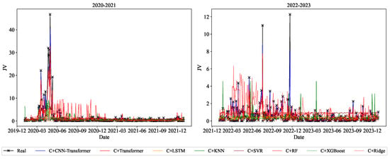
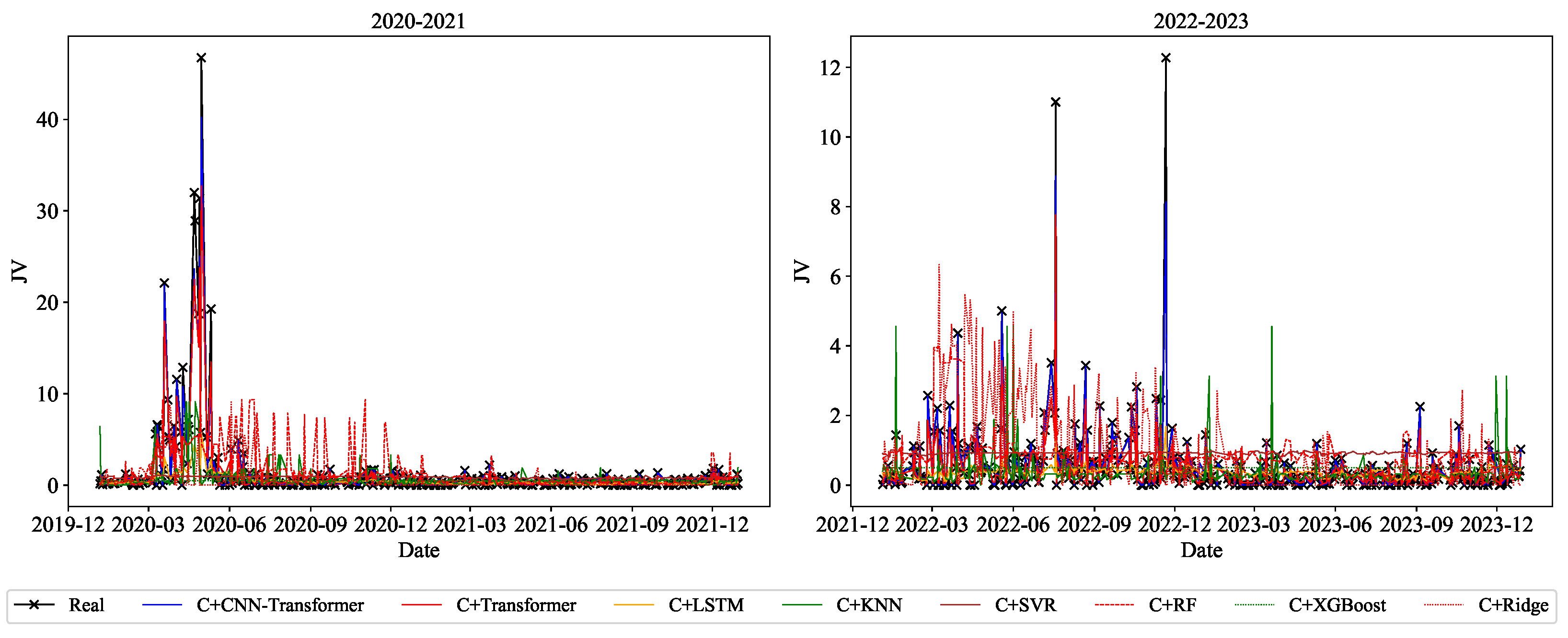
Figure 8 illustrates the fitting performance of various prediction models for jump volatility during 2019–2024. During this period, the C+CNN–Transformer model demonstrates superior ability to capture the peak morphology of the actual values (e.g., 2020–2021), whereas traditional time series models (e.g., C+LSTM, C+KNN) and conventional machine learning models (e.g., C+RF, C+XGBoost) struggle to capture such abrupt fluctuations. Their predicted values are markedly lower than the actual values. In non-extreme intervals, all models show relatively modest deviations from actual values; nevertheless, the C+CNN–Transformer consistently delivers more stable fitting results. Moreover, the C+CNN–Transformer accurately tracks the small-amplitude JV peaks locally observed during 2022–2023. This further validates its potential in forecasting time series that need to capture abrupt dynamics while preserving long-term memory.

Figure 8. The fitting of different models to jump volatility.

To further verify the advantages of the complex network-integrated CNN–Transformer model, this paper conducts one-step and multi-step predictions on JV using the Diebold–Mariano (DM) test, with the results shown in Table 7. It can be observed that the DM statistics are significant at the 0.1% confidence level. If the DM test statistic is positive, the model in the column outperforms the model in the row, and vice versa; the greater the difference between the models, the larger the absolute value of the statistic.

Table 7. Diebold–Mariano tests for forecasting performance (MSE comparison).

(a) Single-Step Forecasting
Model	Comparison Models
	C+XGBoost	C+RF	C+SVR	C+KNN	C+LSTM	C+Transformer	C+CNN–Transformer
C+Ridge	1.877	2.205 **	2.366 **	1.406	4.533 ***	3.237 ***	3.172 ***
C+XGBoost		0.635	1.354	1.137	2.746 ***	2.692 ***	2.681 ***
C+RF			−0.539	−0.547	3.463 ***	3.282 ***	3.204 ***
C+SVR				−0.094	2.906 ***	2.726 ***	2.711 ***
C+KNN					2.370 **	2.724 ***	2.714 ***
C+LSTM						2.673 ***	2.661 ***
C+Transformer							2.517 **
(b) Multi-Step Forecasting
Model	Comparison Models
	C+XGBoost	C+RF	C+SVR	C+KNN	C+LSTM	C+Transformer	C+CNN–Transformer
C+Ridge	2.648 ***	3.334 ***	3.241 ***	3.319 ***	3.545 ***	3.768 ***	3.808 ***
C+XGBoost		9.570 ***	10.008 ***	15.663 ***	10.166 ***	9.523 ***	9.487 ***
C+RF			−1.395	7.292 ***	4.232 ***	4.083 ***	4.051 ***
C+SVR				4.133 ***	4.209 ***	3.447 ***	3.406 ***
C+KNN					3.163 ***	2.928 ***	2.925 ***
C+LSTM						2.730 ***	2.754 ***
C+Transformer							2.805 ***

Note: Residual errors of single-step forecasting values (MSE); and residual errors of multi-step forecasting values (MSE). *** $p<0.001$, ** $p<0.01$.

Overall, the DM statistics between the CNN–Transformer model with complex networks and other comparative models are all positive, indicating that the CNN–Transformer model with complex networks achieves the best performance in one-step predictions. Specifically, the predictive ability of the CNN–Transformer model is significantly superior to that of machine learning models such as RF and SVR. In addition, the predictive ability of the LSTM and Transformer models is better than that of the Ridge Regression, XGBoost, and random forest models. This aligns with findings from previous studies. Notably, a comparison of the CNN–Transformer model’s one-step and multi-step predictions reveals its significant superiority over LSTM (a representative recurrent neural network) and other machine learning models, particularly in long-term forecasting. This further underscores its advantage in capturing long-term nonlinear dependencies.

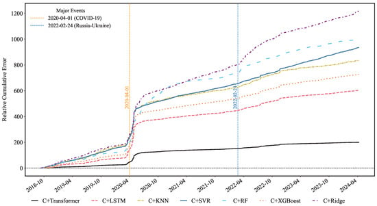
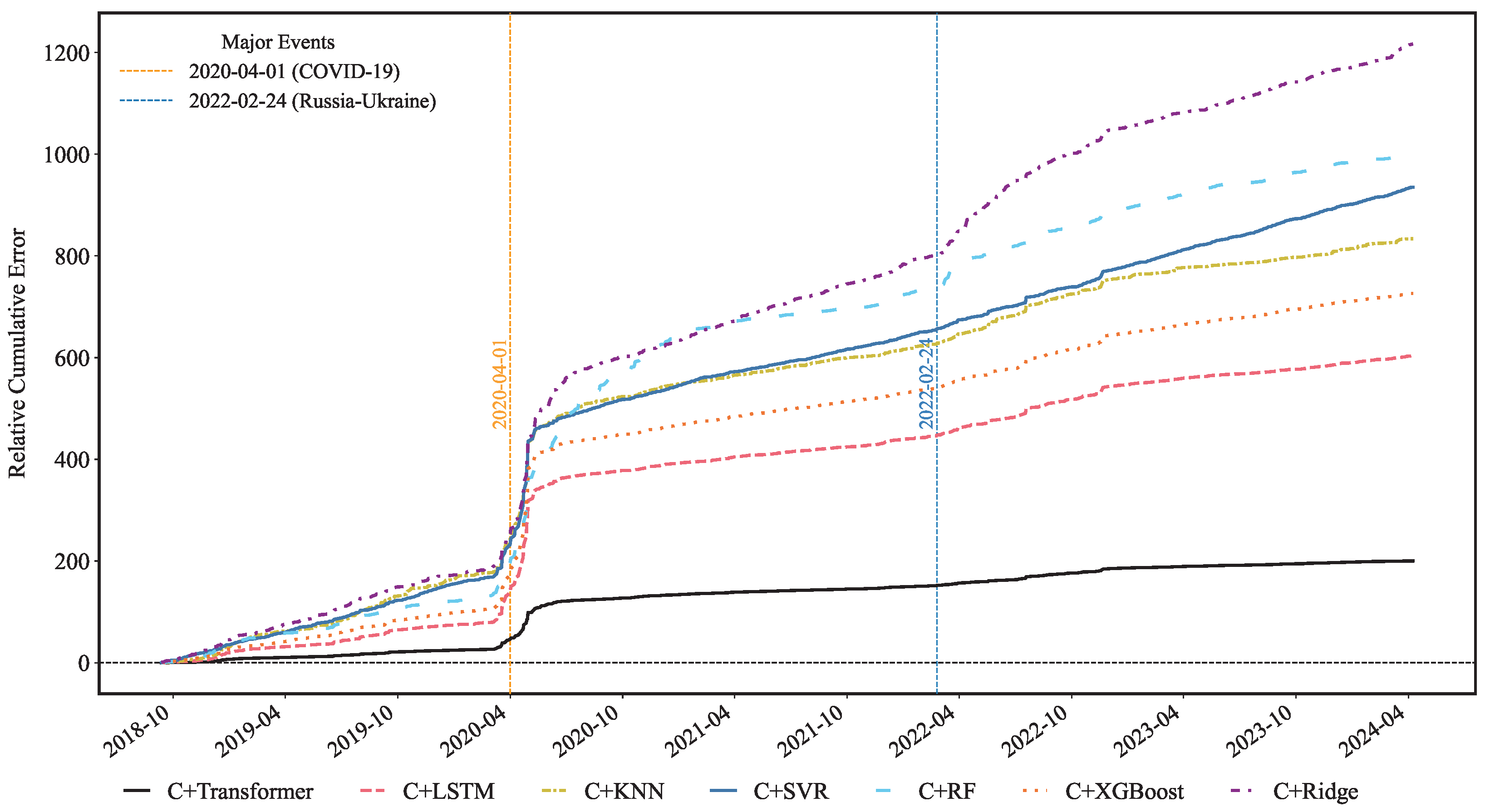
Since financial markets shocked by external events (e.g., Fed rate hikes, geopolitical conflicts, etc.) see surging volatility, model robustness in extreme conditions is critical for risk management. Key moments of sharp jump volatility fluctuations in the past five years, extracted from Figure 3, serve as external shocks to verify whether the CNN–Transformer retains its advantages amid structural market disruptions. Figure 9 shows cumulative relative prediction errors of the CNN–Transformer for WTI jump volatility under different historical lengths, with yellow and blue vertical lines marking COVID-19 and the Russia–Ukraine conflict, respectively. Empirical findings demonstrate that amid market shocks, the CNN–Transformer exhibits the highest robustness among deep learning models. It maintains stable predictive accuracy, thereby enabling effective adaptation to market fluctuations. In contrast, traditional machine learning models struggle to quickly capture market features and respond promptly, resulting in a notable decline in predictive accuracy.

Figure 9. Cumulative relative errors of the C+CNN–Transformer model versus other models.

4. Future Study

Jump intensity, as another core dimension for characterizing discontinuous price jumps in financial markets, and jump volatility jointly underpin critical financial activities such as risk management and asset pricing. Compared with jump volatility, jump intensity focuses on the frequency and dynamic patterns of jumps, which provides a dynamic early warning mechanism for market instability, especially in structural market break periods. Their complementary synergy captures a comprehensive picture of jump characteristics, which is essential for refining jump–diffusion models, monitoring systemic risks, and guiding high-frequency trading risk controls.

Suppose the jump point process $J\left(t\right)$ follows the Hawkes point process with intensity ${\lambda }^{*}\left(t\right)$:

$${\lambda }^{*}\left(t\right)=\lambda +\sum _{t_i<t}\mu \left(t-t_i\right)$$

where $\mu$ is called the (exciting) kernel of the process; a common choice is an exponential decay function:

$${\lambda }^{*}\left(t\right)=\lambda +{\int }_0^t\alpha {\mathrm{e}}^{-\beta (t-s)}\mathrm{d}N\left(s\right)=\lambda +\sum _{t_i<t}\alpha {\mathrm{e}}^{-\beta \left(t-t_i\right)}$$

the maximum likelihood estimator ($\widehat{\lambda },\widehat{\alpha },\widehat{\beta }$) can be obtained by

$$\left(\widehat{\lambda },\widehat{\alpha },\widehat{\beta }\right)=argmaxL\left(\lambda ,\alpha ,\beta \right)$$

where the likelihood function

$$\ell =\sum _{i=1}^{n\left(T\right)}ln\left[\lambda +\alpha \sum _{j=1}^{i-1}{\mathrm{e}}^{-\beta \left(t_i-t_j\right)}\right]-\lambda T-{\displaystyle \frac{\alpha }{\beta }}\sum _{i=1}^{n\left(T\right)}\left[1-{\mathrm{e}}^{-\beta \left(T-t_i\right)}\right]$$

the daily jump intensity can be expressed as

$${\lambda }_d^{*}={\widehat{\lambda }}_d+\sum _{t_{i,d}<t_d}{\widehat{\alpha }}_d{\mathrm{e}}^{-{\widehat{\beta }}_d\left(t_d-t_{i,d}\right)}$$

where ${\lambda }_d^{*}$ represents the d th day and i represents the i th jump moment on the d-th day.

Table 8 presents the performance comparison of various models integrated with topological characteristics of complex networks in the one-step prediction task of financial jump intensity. From the overall indicators, the CNN–Transformer model demonstrates remarkable advantages: its prediction accuracy is relatively optimal among all models, and the low degree of dispersion ensures that the prediction results have good stability. In the scenario of risk assessment, relying on its excellent performance across multiple indicators, this model can provide more reliable decision-making bases for financial institutions to set risk reserves and implement risk management and control of investment portfolios. This echoes the research conclusions on jump volatility mentioned earlier, fully verifying that the indicator system constructed in this paper, as well as the model architecture integrating deep learning, can output high-quality prediction performances in the analysis of both financial jump amplitude and jump frequency, effectively supporting the accurate judgment of the financial market.

Table 8. Model performance comparison for prediction.

Model	RMSE	MAE	SMAPE	MSLE	MBE	SD
C+CNN–Transformer	0.8032	0.6080	0.2680	0.1179	−0.6279	0.4250
C+Transformer	0.8542	0.6689	0.2904	0.1490	−0.3061	0.4263
C+LSTM	0.8808	0.6826	0.2938	0.1202	−0.5056	0.4271
C+KNN	0.8937	0.7023	0.3025	0.1320	−1.0465	0.4438
C+SVR	0.9310	0.6953	0.3033	0.1423	−0.4902	0.4486
C+RF	0.8722	0.6856	0.2950	0.1220	−0.8019	0.4343
C+XGBoost	0.9579	0.8192	0.3437	0.1670	0.3347	0.4271
C+Ridge	1.0950	0.8643	0.3544	0.1899	0.7726	0.5403

Note: “C+” indicates the addition of topological characteristics of complex networks as forecasting indicators to the basic model.

From an economic perspective, the superior performance of the CNN–Transformer model is closely aligned with real financial market dynamics: Specifically, in risk assessment scenarios, relying on its excellent performance across multiple indicators, the model can provide more reliable decision-making support for financial institutions to set risk reserves and implement portfolio risk management—directly reducing potential economic losses caused by extreme jump events (e.g., sudden geopolitical shocks or commodity price fluctuations). Additionally, the model’s accurate prediction of jump intensity reflects the sensitivity to core economic drivers (e.g., changes in OVX, geopolitical risk indices, and cross-market capital flows). This enables it to capture the economic logic behind jump dynamics, rather than merely achieving statistical fitting. This echoes the earlier research conclusions on jump volatility, fully verifying that the constructed indicator system and the deep learning-integrated model architecture can deliver high-quality prediction performance in both financial jump amplitude and frequency analysis. More importantly, the model’s economic relevance ensures its practical applicability, effectively supporting accurate judgment and decision-making in financial markets.

5. Discussion

5.1. Contribution of Features

To further verify the contribution of different indicators to the improvement in predictive performance, we conduct an ablation-style analysis to enhance the interpretability of the results. Table 9 presents the outcomes of the ablation experiment, from which we can observe that the inclusion of Energy Information and Geopolitical Risk leads to the most substantial reduction in prediction errors. From an economic perspective, as a typical commodity, the production, storage, and consumption of crude oil serve as the core anchors of long-term supply–demand dynamics. Market participants incorporate expectations of annual production contraction or expansion into short-term trading decisions; for example, expectations of insufficient annual supply will trigger short-term hoarding behavior, thereby amplifying abrupt price fluctuations. Moreover, crude oil supply is highly dependent on geopolitical stability, as rising geopolitical risk intensifies market concerns about supply disruptions, which in turn triggers short-term panic trading.

Table 9. Effects of feature omission on prediction errors (ER = Error Ratio of Increase).

Absent Feature	RMSE	ER	MAE	ER	SMA PE	ER	MSLE	ER	MBE	ER	SD	ER
No Absence	2.4538	100.00%	0.6826	100.00%	1.0147	100.00%	0.1614	100.00%	−0.1924	100.00%	2.4463	100.00%
Complex Network	2.8134	14.65%	0.7382	8.15%	1.5368	51.46%	0.3220	99.49%	−0.7212	274.92%	2.7194	11.16%
Trading Information	2.8091	14.48%	0.7296	6.89%	1.4383	41.75%	0.3121	93.35%	−0.7043	266.14%	2.7194	11.16%
Market Sentiment	2.8064	14.37%	0.7535	10.40%	1.4980	47.63%	0.3210	98.88%	−0.6553	240.67%	2.7288	11.55%
Financialization	2.7389	11.62%	0.8512	24.70%	1.1749	15.79%	0.2842	76.11%	−0.1610	−16.33%	2.7342	11.77%
Economic Policy Uncertainty	2.7987	14.05%	0.7681	12.53%	1.4640	44.28%	0.3184	97.25%	−0.6120	218.14%	2.7310	11.64%
Geopolitical Risk	2.8241	15.09%	0.7620	11.64%	1.6327	60.91%	0.3488	116.11%	−0.7619	296.08%	2.7194	11.16%
Energy Information	3.0081	22.59%	1.9087	179.65%	1.4466	42.57%	0.7977	394.25%	1.2859	568.47%	2.7194	11.16%
P	2.9064	18.44%	1.6785	145.91%	1.4014	38.12%	0.6702	315.27%	1.0256	433.15%	2.7194	11.16%
L	2.7728	13.00%	1.2387	81.48%	1.2824	26.39%	0.4363	170.35%	0.4995	159.68%	2.7275	11.49%
S	2.8217	14.99%	1.1750	72.15%	1.2494	23.13%	0.4351	169.55%	0.3208	66.75%	2.8034	14.60%
C	2.8241	15.09%	0.7620	11.64%	1.6307	60.71%	0.3488	116.11%	−0.7620	296.10%	2.7194	11.16%

Additionally, adding network features also brings about a considerable improvement in reducing prediction errors, which echoes empirical viewpoints on the impacts on predictive performance. In order to more precisely assess the contribution of each network feature, we further disaggregated the features of the network structure. It was found that the inclusion of Network Average Degree Centrality (P) led to the greatest improvement in performance. As an indicator measuring the connectivity among features, Network Average Degree Centrality (P) not only reflects the information transmitted between features but also captures the impact of features on extreme fluctuations in a timely manner, thus contributing the most significantly to the predictive improvement in jump volatility. Moreover, path length (L) and closeness centrality (C) reflect the path and convenience of information transmission, and their absence weakens the model’s ability to capture market linkage shocks. Strength (S) depicts the intensity of feature correlation, which makes a marginal contribution to the transmission of short-term jump information. By characterizing the linkage structure between market information, these network indicators enable the capture of extreme fluctuation transmission, thereby enhancing the accuracy of jump volatility prediction.

5.2. Model Validity

In this paper, we adopt miceforest imputation as the method for handling mixed-frequency data. The following sections will discuss both economic validity and model comparison.

(1)

Economic Rationality of Data Imputation Methods: In this study, missing values in mixed-frequency data mainly result from practical scenarios such as financial market closures and data transmission delays. These missing values are random and closely related to the economic correlations between variables. From an economic logic perspective, financial variables (e.g., GEPU, GPR series indicators) exhibit significant nonlinear correlations and dynamic transmission effects (e.g., sudden geopolitical risk shocks indirectly affect crude oil volatility through market expectations). MICEForest interpolation, based on the random forest algorithm, can capture the complex nonlinear dependencies between variables, which is consistent with the economic nature of multi-factor interactions in financial markets. In contrast, linear interpolation assumes a simple linear relationship between variables, which fails to reflect the real dynamic correlations of financial data. This is also verified by the performance indicators in the table: MICEForest interpolation outperforms linear interpolation in core error metrics such as RMSE (2.4538), MAE (0.6826), and SMAPE (1.0147), confirming its dual rationality in economic logic and prediction accuracy.

(2)

We have conducted robustness tests based on existing data, and the results in Table 10 are as follows: By comparing core performance indicators of MICEForest interpolation and linear interpolation, MICEForest achieves a 13–37% improvement in key error metrics such as RMSE, MAE, and SMAPE. Additionally, its MSLE (0.1614) is significantly lower than that of linear interpolation (0.3488), indicating that its prediction accuracy for jump volatility (JV) is more stable and not significantly affected by data distribution characteristics.

Table 10. Comparison of interpolation model prediction results.

Model	RMSE	MAE	SMAPE	MSLE	MBE	SD
miceforest Interpolation	2.4538	0.6826	1.0147	0.1614	−0.1924	2.4463
Linear Interpolation	2.8241	0.7620	1.6307	0.3488	−0.7620	2.7194

5.3. Limitations

Our study has two limitations:

(1)

Given the absence of a widely accepted unified benchmark model in the existing literature, we restricted our comparisons to prevailing mainstream models. As a result, the optimality of our proposed model is confined to the single-model framework. In future work, we will explore approaches to develop a globally optimal model.

(2)

This study adopts a fixed hyperparameter strategy in the rolling window forecasting framework without frequent re-optimization. First, frequent hyperparameter re-optimization may cause the model to overfit the noise characteristics of local window data, thereby reducing its generalization ability for future data prediction. Additionally, fixed hyperparameters can significantly lower the computational cost during the rolling forecasting process, improve forecasting efficiency, and better align with the real-time forecasting requirements of actual financial markets. However, this study has not explored the stability of hyperparameters across rolling windows nor adopted a strategy of frequent hyperparameter re-optimization. This limitation may result in the inability to fully rule out the potential risk of the adaptability of hyperparameters diminishing in specific market phases.

6. Conclusions and Extension

This study focuses on jump volatility in financial markets, using it as a proxy variable for jump risk to conduct predictive research. We construct a predictive indicator system integrated with complex network characteristics. Additionally, a CNN–Transformer hybrid model is proposed to combine the local feature extraction capability of CNNs and the self-attention mechanism of Transformers. To ensure the robustness of the findings, this study further employs multi-dimensional evaluation indices, Diebold–Mariano (DM) tests, and shock experiments for comprehensive analysis. Extensions to jump intensity also confirm the model’s general applicability.

The key research conclusions of this study are as follows:

(i)

A comprehensive predictive indicator system was constructed. Beyond covering the core information required for jump volatility prediction, this system effectively captures the associative relationships and structural characteristics of jump dynamics by incorporating complex network features among indicators—laying a solid foundation for enhancing jump volatility prediction performance.

(ii)

Empirical results show that the CNN–Transformer model proposed in this study achieves the highest prediction accuracy in both one-step and multi-step jump volatility forecasting, significantly outperforming traditional econometric models, machine learning models, and conventional deep learning models. The synergistic effect of the CNN module and attention mechanism enables the model to maintain high prediction accuracy even when the forecasting horizon is extended, addressing the issue of accuracy degradation in multi-step forecasting of traditional models.

(iii)

The CNN–Transformer model exhibits excellent robustness. Comparison of model performance via Diebold–Mariano (DM) tests reveals that the DM test statistics of the CNN–Transformer model are all positive. This result not only confirms the model’s superiority in long-term forecasting but also verifies its stability. Further shock experiments demonstrate that the model maintains stable performance in extreme market jump scenarios (e.g., jumps caused by sudden policy changes or liquidity crises), indicating that the model constructed in this study is more adaptable to the suddenness and extremeness of data than traditional models.

(iv)

This study conducted model validation focusing on the two core dimensions—jump volatility and jump intensity. The validation results consistently show that the CNN–Transformer model can fully adapt to the complexity of jump features, confirming its versatility and effectiveness in jump-related prediction tasks.

Future research can focus on the integration of text information mining and jump volatility prediction. This will expand the models’ cross-market prediction capability, thereby providing more refined quantitative support for timing high-frequency trading strategies and hedging cross-market portfolio risks.

References

- Black, F.; Scholes, M. The pricing of options and corporate liabilities. J. Political Econ. 1973, 81, 637–654. [Google Scholar] [CrossRef] [Scilit]
- Engle, R.F. Autoregressive conditional heteroscedasticity with estimates of the variance of united kingdom inflation. Econom. J. Econom. Soc. 1982, 50, 987–1007. [Google Scholar] [CrossRef] [Scilit]
- Bollerslev, T. Generalized autoregressive conditional heteroscedasticity. J. Econom. 1986, 31, 307–327. [Google Scholar] [CrossRef] [Scilit]
- Corsi, F. A simple approximate long-memory model of realized volatility. J. Financ. Econom. 2009, 7, 174–196. [Google Scholar] [CrossRef] [Scilit]
- Andersen, T.G.; Bollerslev, T.; Diebold, F.X. Roughing it up: Including jump components in the measurement, modeling, and forecasting of return volatility. Rev. Econ. Stat. 2007, 89, 701–720. [Google Scholar] [CrossRef] [Scilit]
- Corsi, F.; Renò, R. Discrete-time volatility forecasting with persistent leverage effect and the link with continuous-time volatility modeling. J. Bus. Econ. Stat. 2012, 30, 368–380. [Google Scholar] [CrossRef] [Scilit]
- Bollerslev, T.; Patton, A.J.; Quaedvlieg, R. Exploiting the errors: A simple approach for improved volatility forecasting. J. Econom. 2016, 192, 1–18. [Google Scholar] [CrossRef] [Scilit]
- Patton, A.J.; Sheppard, K. Good volatility, bad volatility: Signed jumps and the persistence of volatility. Rev. Econ. Stat. 2015, 97, 683–697. [Google Scholar] [CrossRef] [Scilit]
- Sun, H.; Li, X.; Li, Z.; Fu, Q. Functional volatility relationship analysis and prediction in international crude oil futures markets. J. Futur. Mark. 2024, 44, 1581–1612. [Google Scholar] [CrossRef] [Scilit]
- Dutta, A.; Bouri, E. Forecasting the volatility of crude oil futures: New evidence from jump-induced volatility. Energy Strategy Rev. 2024, 56, 101588. [Google Scholar] [CrossRef] [Scilit]
- Yang, J.; Zhou, Y. Return and volatility transmission between China’s and international crude oil futures markets: A first look. J. Futur. Mark. 2020, 40, 860–884. [Google Scholar] [CrossRef] [Scilit]
- Luong, C.; Dokuchaev, N. Forecasting of realised volatility with the random forests algorithm. J. Risk Financ. Manag. 2018, 11, 61. [Google Scholar] [CrossRef] [Scilit]
- Demirer, R.; Gkillas, K.; Gupta, R.; Pierdzioch, C. Risk aversion and the predictability of crude oil market volatility: A forecasting experiment with random forests. J. Oper. Res. Soc. 2022, 73, 1755–1767. [Google Scholar] [CrossRef] [Scilit]
- Kumbure, M.M.; Lohrmann, C.; Luukka, P.; Porras, J. Machine learning techniques and data for stock market forecasting: A literature review. Expert Syst. Appl. 2022, 197, 116659. [Google Scholar] [CrossRef] [Scilit]
- Xu, C.; Li, J.; Feng, B.; Lu, B. A financial time-series prediction model based on multiplex attention and linear transformer structure. Appl. Sci. 2023, 13, 5175. [Google Scholar] [CrossRef] [Scilit]
- Wei, Y.; Xu, K.; Yao, J.; Sun, M.; Sun, Y. Financial risk analysis using integrated data and transformer-based deep learning. J. Comput. Sci. Softw. Appl. 2024, 4, 1–8. [Google Scholar]
- Jia, F.; Yang, B. Forecasting volatility of stock index: Deep learning model with likelihood-based loss function. Complexity 2021, 2021, 5511802. [Google Scholar] [CrossRef] [Scilit]
- Zhang, C.-X.; Li, J.; Huang, X.-F.; Zhang, J.-S.; Huang, H.-C. Forecasting stock volatility and value-at-risk based on temporal convolutional networks. Expert Syst. Appl. 2022, 207, 117951. [Google Scholar] [CrossRef] [Scilit]
- Thakkar, A.; Chaudhari, K. A comprehensive survey on deep neural networks for stock market: The need, challenges, and future directions. Expert Syst. Appl. 2021, 177, 114800. [Google Scholar] [CrossRef] [Scilit]
- Jemitkumar, P.P.; Harsh, S.; Rashmi, B. Predicting implied volatility using deep learning for option pricing. Res. Sq. 2025. [Google Scholar] [CrossRef] [Scilit]
- Jung, G.; Choi, S.-Y. Forecasting foreign exchange volatility using deep learning autoencoder-LSTM techniques. Complexity 2021, 2021, 6647534. [Google Scholar] [CrossRef] [Scilit]
- Petrozziello, A.; Troiano, L.; Serra, A.; Jordanov, I.; Storti, G.; Tagliaferri, R.; La Rocca, M. Deep learning for volatility forecasting in asset management. Soft Comput. 2022, 26, 8553–8574. [Google Scholar] [CrossRef] [Scilit]
- Liu, Y. Novel volatility forecasting using deep learning–long short term memory recurrent neural networks. Expert Syst. Appl. 2019, 132, 99–109. [Google Scholar] [CrossRef] [Scilit]
- Li, P.; Wang, B. An approach to hang seng index in hong kong stock market based on network topological statistics. Chin. Sci. Bull. 2006, 51, 624–629. [Google Scholar] [CrossRef] [Scilit]
- Liu, C.; Arunkumar, N. Risk prediction and evaluation of transnational transmission of financial crisis based on complex network. Clust. Comput. 2019, 22, 4307–4313. [Google Scholar] [CrossRef] [Scilit]
- Ouyang, F.-Y.; Zheng, B.; Jiang, X.-F.; Podobnik, B. Intrinsic multi-scale dynamic behaviors of complex financial systems. PLoS ONE 2015, 10, e0139420. [Google Scholar] [CrossRef] [Scilit]
- Saeedian, M.; Jamali, T.; Kamali, M.Z.; Bayani, H.; Yasseri, T.; Jafari, G.R. Emergence of world-stock-market network. Phys. A Stat. Mech. Its Appl. 2017, 526, 120792. [Google Scholar] [CrossRef] [Scilit]
- Barndorff-Nielsen, O.E.; Shephard, N. Power and Bipower Variation with Stochastic Volatility and Jumps. J. Financ. Econom. 2004, 2, 1–37. [Google Scholar] [CrossRef] [Scilit]
- Cao, H.; Lin, T.; Li, Y.; Zhang, H. Stock price pattern prediction based on complex network and machine learning. Complexity 2019, 2019, 4132485. [Google Scholar] [CrossRef] [Scilit]
- Diebold, F.X.; Mariano, R.S. Comparing predictive accuracy. J. Bus. Econ. Stat. 2002, 20, 134–144. [Google Scholar] [CrossRef] [Scilit]
- Kong, A.; Zhu, H.; Azencott, R. Predicting intraday jumps in stock prices using liquidity measures and technical indicators. J. Forecast. 2021, 40, 416–438. [Google Scholar] [CrossRef] [Scilit]
- Mäkinen, Y.; Kanniainen, J.; Gabbouj, M.; Iosifidis, A. Forecasting jump arrivals in stock prices: New attention-based network architecture using limit order book data. Quant. Financ. 2019, 19, 2033–2050. [Google Scholar] [CrossRef] [Scilit]
- Ntakaris, A.; Magris, M.; Kanniainen, J.; Gabbouj, M.; Iosifidis, A. Benchmark dataset for mid-price forecasting of limit order book data with machine learning methods. J. Forecast. 2018, 37, 852–866, Erratum in J. Forecast. 2020, 39, 707. [Google Scholar] [CrossRef] [Scilit]
- Arellano, C.; Bai, Y.; Kehoe, P.J. Financial frictions and fluctuations in volatility. J. Political Econ. 2019, 127, 2049–2103. [Google Scholar] [CrossRef] [Scilit]
- Tabash, M.I.; Issa, S.S.; Mansour, M.; Saleh, M.W.; Rahrouh, M.; AlQeisi, K.; Al-Absy, M.S.M. Dynamic Shock-Transmission Mechanism Between US Trade Policy Uncertainty and Sharia-Compliant Stock Market Volatility of GCC Economies. Risks 2025, 2, 66–76. [Google Scholar]
- Zhang, X.; Zhou, J.; Du, X. Impact of oil price uncertainty shocks on China’s macro-economy. Resour. Policy 2022, 79, 103080. [Google Scholar] [CrossRef] [Scilit]
- Punzi, M.T. The impact of energy price uncertainty on macroeconomic variables. Energy Policy 2019, 129, 1306–1319. [Google Scholar] [CrossRef] [Scilit]
- Shah, A.D.; Bartlett, J.W.; Carpenter, J.; Nicholas, O.; Hemingway, H. Comparison of random forest and parametric imputation models for imputing missing data using MICE: A CALIBER study. Am. J. Epidemiol. 2014, 179, 764–774. [Google Scholar] [CrossRef] [Scilit]
- Wei, Y. Volatility forecasting models for CSI 300 index futures. J. Manag. Sci. China 2010, 2, 66–76. [Google Scholar]
Disclaimer/Publisher’s Note: The statements, opinions and data contained in all publications are solely those of the individual author(s) and contributor(s) and not of MDPI and/or the editor(s). MDPI and/or the editor(s) disclaim responsibility for any injury to people or property resulting from any ideas, methods, instructions or products referred to in the content. |
© 2026 by the authors. Licensee MDPI, Basel, Switzerland. This article is an open access article distributed under the terms and conditions of the Creative Commons Attribution (CC BY) license.