


Abstract
In empirical sciences, the inductive construction of mathematical models relies on observations from controlled experiments, yet the conditions under which such constructions yield well-defined deterministic dynamics remain largely implicit. Within the framework of Axiomatic System Dynamics (ASD), this paper develops an algebraic theory of inductive mathematical modeling based on an ontological–epistemological dual structure. The modeling domain (MD) is formalized as a mathematical structure encoding initial conditions, loading protocols, and admissible loading ranges, thereby characterizing model applicability and the mechanisms of failure under improper extrapolation. Weak and strong validity conditions characterize, respectively, the uniqueness and dynamical closure of observable parameter evolution, yielding an algebraic constraint structure for mathematical models and their induced state-space representations. Generalized state parameters incorporate loading-history information, and an existence theorem is established. Difference representations of states and parameters provide an algebraic basis for expressing the underlying logic of comparative experiments, controlled-variable methods and causal inference. Together, these constructions formalize otherwise implicit concepts and structures in conventional modeling practice, render them amenable to algebraic reasoning, and provide a unified theoretical foundation for future extensions.
Keywords:
inductive mathematical modeling; Axiomatic System Dynamics (ASD); modeling domain; observable parameter; dynamical closure; validity condition; state parameter; state-space representation; generalized state parameter MSC:
93A30; 93A05; 37N35; 93B25
1. Introduction
Despite the diversity of research objects, system properties, and mathematical formulations across the natural sciences, the essence of mathematical modeling may ultimately be viewed as the quantitative characterization of system properties and their evolutionary laws.
From the perspective of modern systems science, a broad class of deterministic mathematical models can be represented within the framework of state-space theory [1,2,3] by the following system of equations:
Here, the state equation describes the evolution of the state variable x under the input u, while the observation equation maps the state x to the corresponding observable output y. Through this formulation, the evolutionary behavior of the property of interest (y) driven by external actions is characterized, thereby fulfilling the objective of mathematical modeling.
Grounded in state-space theory, systems science has developed a spectrum of theoretical branches and analytical tools: system identification [4,5,6,7] addresses the construction of system models and the estimation of their parameters from observational data; (latent) state representation learning [8,9,10,11] seeks to extract dynamically meaningful state representations from empirical data; behavioral systems theory [12,13,14] dispenses with the conventional causal input-output paradigm, taking system behavior at the center of analysis; factor dynamics [15,16], together with behavioral equivalence [17,18], employs quotient maps and dynamical commutation relations to characterize the preservation of dynamics, order reduction, and equivalence across distinct state representations.
Concurrently, with respect to the formalization of mathematical models per se, Mesarovic and Takahara [19] developed a formal foundation for general systems theory based on set algebra; Takahashi and Takahara [20] formulated a logical systems-theoretic methodology for the formal description of heterogeneous models; Zeigler [21,22] established the formal modeling and simulation framework of the discrete event system specification (DEVS). Collectively, these developments have substantially broadened the mathematical foundations of modern systems science and its related areas.
Nevertheless, in the empirical sciences and engineering, the system under investigation is typically regarded as an objectively existing entity governed by underlying dynamical laws that are independent of the observer. The researcher can neither fully access the system’s ontological state nor exhaust its internal information. Accordingly, the inductive construction of a mathematical model proceeds through an epistemological process: controlled experiments prescribe initial conditions and loading protocols or control interventions, while the resulting evolutionary behavior of observable parameters (such as stress, strain, and temperature) is measured and recorded. These observations, together with the imposed experimental constraints, provide the basis for inferring deterministic mathematical relations or dynamical equations.
Consequently, the inductive modeling process can be formalized, within the state-space framework, as the ontological–epistemological dual structure illustrated in Figure 1a.
Figure 1.
(a) Ontological–epistemological dual structure of system evolution. (b) Modeling domain (MD). System evolution in controlled experiments is deterministic and reproducible in the sense of set-valued state evolution.
At the ontological dynamics layer, the equation Sk+1 = F(Sk, Uk) describes the evolution of the system’s ontological state S ∈ driven by the ontological input U ∈ , thereby representing the underlying dynamical laws governing the system.
At the epistemological observation and modeling layer, x ∈ X, y ∈ Y denote observable parameters of the system, each formalized as a projection of the state S, where the projection maps πx, πy are determined by the corresponding parameter types. Similarly, u ∈ * denotes the encoding of the loading protocol (e.g., “increase by 1 kPa” or “decrease by 1 °C”), formalized as a projection of the ontological input U ∈ , where the projection map πu is determined by the designated loading protocol and its encoding scheme.
In each trial of a controlled experiment, a prescribed loading path is applied to the system, giving rise to the corresponding observed parameter evolutions . These sequences do not constitute the system’s ontological dynamics itself; rather, they are epistemological projections of the underlying dynamics realized under the specified experimental configuration.
The scope of a controlled experiment can be formalized as a modeling domain , as illustrated in Figure 1b. Here, * denotes the selected loading protocol together with its encoding scheme, while 0 ⊆ denotes the prescribed initial condition. In experimental practice, it is generally impossible to constrain the initial ontological state S0 to a single value; rather, given the finite information available about the initial condition, one can only restrict it to a specific subset of the state space, namely S0 ∈ 0. Furthermore, denotes the loading scope, defined as the set of all admissible loading paths .
Given that 0 constitutes a subset of the state space , and that an individual encoding uk can, at most, constrain the ontological input Uk to a specific fiber , the evolution of the system under a prescribed loading path is deterministic and reproducible only in the sense of set-valued state evolution .
Consequently, within the context of controlled experiments, the inductive construction of a deterministic mathematical model gives rise to the following fundamental questions:
- Is the evolutionary behavior of the observed parameters unique across repeated trials? That is, does the loading path uniquely determine the evolutionary paths ?
- Does a given parameter contain sufficient information to determine its own evolution, thereby qualifying as a valid state variable? That is, does there exist a well-defined dynamical equation xk+1 = f(xk, uk)?
- Does a single-valued mapping relation hold between the two types of parameters? Specifically, does there exist a function yk = g(xk)?
- How does the choice of the modeling domain MD affect these algebraic properties?
It is evident that these criteria do not presuppose the validity of Equation (1); rather, they characterize the conditions under which a state-space representation can be established. This leads to the fundamental meta-modeling question addressed in this paper: under what algebraic and topological conditions does an observable parameter admit a well-defined, single-valued, and deterministic dynamical characterization?
Existing theories provide a broad range of mathematical tools for analyzing system structure, behavior, and representation, but generally take the relevant mathematical structures as given. By contrast, inductive mathematical modeling seeks to construct such structures from observations, loading controls, and initial condition constraints imposed on an objectively existing system.
This construction is organized by the modeling domain (MD), which specifies the admissible experimental configurations within which a mathematical model is constructed and its validity is evaluated. Although the MD is epistemological in nature, its specification determines the algebraic properties exhibited by observable parameters within the domain and, consequently, constrains the form and domain of applicability of the resulting mathematical model.
In conventional modeling practice, however, the MD is typically specified through empirical heuristics and lacks a unified mathematical formulation. A rigorous formalization of the MD and the inductive modeling process would provide a theoretical basis for understanding how deterministic mathematical models are constructed from ontological dynamics through controlled experimentation. It would also provide an operational framework for designing experiments that are informative and computationally tractable.
Motivated by these considerations, our previous work established the meta-modeling framework of Axiomatic System Dynamics (ASD) [23]. Within this framework, ontological dynamics are represented by conceptual models composed of generalized constitutive relationships (GCRs), which encode causal relations in a minimal “state-action-state increment” form. Mathematical models are formulated as mathematical realizations of the corresponding conceptual models.
However, although the core concepts underlying this ontological–epistemological dual structure—including the ontological state, epistemological parameter, internal/external actions, state parameter, and action quantification—were introduced in the previous work, they have so far been formulated through descriptive definitions rather than rigorous algebraic characterizations.
Following the principle of minimal mathematical structure, this paper develops an algebraic theory of inductive mathematical modeling within the ASD framework. The theory formalizes the construction of deterministic mathematical models from controlled experiments, establishes algebraic criteria for the uniqueness and dynamical closure of observable parameter evolution, and makes explicit the algebraic structures underlying conventional modeling practice.
The primary focus of this work is the formalization of the inductive modeling process itself, rather than a specific model-construction algorithm. Accordingly, the present study is restricted to a deterministic setting and does not consider stochastic noise, measurement errors, or other sources of uncertainty. Nevertheless, the framework provides a foundation for future extensions and offers a complementary perspective on state-space modeling grounded in ASD’s analysis of causal structure.
2. Ontological Dynamics Layer
2.1. Ontological Dynamics Structure
Within the mathematical modeling framework of Axiomatic System Dynamics (ASD), the evolution of a system is grounded in the ontological dynamics structure. This structure is defined as the tuple:
The relationships among its core concepts are illustrated in Figure 2.
C(0) = (T, dt, , , L, gi, e)
Figure 2.
Ontological dynamics structure and the one-step evolution of the system state over a basic evolution interval.
Let T ⊆ ℝ denote the time domain, with element t ∈ T termed a time point. Let dt ∈ ℝ+ denote the characteristic time scale. Any interval
is referred to as a basic evolution interval.
It = [t,t + dt], t,t + dt ∈ T
Within the ASD framework, the evolution law of the system state is defined on each basic evolution interval It and is independent of the temporal base point t. Accordingly, all dynamical operators introduced subsequently (e.g., L and gi) are assumed to satisfy time-translation invariance. For simplicity, we restrict attention to the idealized setting in which T = ℝ, and dt is a prescribed constant.
At the ontological dynamics layer, except for the time domain T and the characteristic time scale dt, all other components of the tuple C(0) are assigned ontological status. More precisely, although their mathematical structures are assumed to exist objectively and uniquely, they are epistemically inaccessible; their specific mathematical forms cannot be determined by direct observation and are therefore treated as abstract system entities independent of any particular observation or measurement procedure.
Let denote the state space, with each S ∈ called a state. The state S encapsulates the complete information of the system, sufficient to determine its evolution under any action, and exists uniquely at any given instant t.
Let denote the action space, with each F ∈ called an action. The action F constitutes the sole factor that changes the system state, and exists uniquely within any basic evolution interval It.
The function
is called the ontological dynamics operator. It characterizes the system’s ontological dynamics, formulated as
This equation constitutes the rigorous algebraic realization of ASD Axiom 1. It dictates that the state S at time t, together with the total action F exerted over It, uniquely determines the updated state S′ at time t + dt.
L: × →
S × F ↦ S′
S × F ↦ S′
S′ = L(S, F)
More fundamentally, this equation constitutes the minimal causal unit of ASD causal-structure analysis. Here, S represents the entity that undergoes change, F represents the cause of the change, and the transition from S to S′ characterizes the resulting change. This unit serves as the building block from which more complex causal relations can be constructed and analyzed.
The function
is called the internal action generation operator. The element in the action space
is termed the internal action, characterizing the endogenous driving factor for the system’s spontaneous evolution. This equation constitutes the rigorous algebraic realization of ASD Axiom 2, signifying that the state S at time t uniquely determines the internal action Fi over the interval It.
gi: →
S ↦ Fi
S ↦ Fi
Fi = gi(S)
Let e = Map(, ) denote the external action space, defined as the set of all transformations on the action space . Its element Fe ∈ e, termed the external action, characterizes the exogenous driving factor for the system’s evolution and exists uniquely within any basic evolution interval It.
Algebraically, the external action Fe manifests as a mapping and shift applied to the internal action Fi. Consequently, the total action F exerted upon the system is formulated as the application of the external action to the internal action:
F = Fe(Fi)
Combining the preceding definitions, over any basic evolution interval It, the ontological dynamics equation is ultimately formulated as
which characterizes the evolution of the system state on a discrete time scale.
S′ = L(S,Fe(gi(S)))
Furthermore, given an initial state S0 and a sequence of external actions , the corresponding state sequence can be uniquely constructed by the recursion:
This induces the state path generation operator
yielding
Provided the initial state S0 corresponds to the initial time t0, the system state at any subsequent time tk = t0 + kdt, k ∈ ℕ is given by Sk in the above sequence.
Sk+1 = L(Sk, Fe,k(gi(Sk))), k ∈ ℕ
In summary, the ontological dynamics structure C(0) represents the objectively existing system investigated through experiments and provides the causal backbone of its evolution. In what follows, C(0) assumed to be given.
2.2. Difference Representation of the State
The variation in the system state can be described by an appropriate algebraic structure. We define a difference representation of the state as the triple:
The relationships among its core concepts are illustrated in Figure 3a.
((, +), d, ⊕)
Figure 3.
(a) Difference representation of the state. (b) The induction principle of external actions (B-A principle) in ASD. The net contribution of an external action is identified through differences between comparative experiments.
Let the abelian group (, +) denote the state increment space, whose element dS ∈ is called the state increment, with the additive identity of the group denoted by 0dS. The function
is called the state difference operator. For ∀S ∈ , the induced map
is a bijection. Moreover, for ∀S, S′, S″ ∈ , Chasles’ relation holds:
This uniquely induces the map
called the state update operator. Its operation S′=⊕(S, dS) can be denoted as
d: × →
S × S′ ↦ dS
S × S′ ↦ dS
dS: →
S′ ↦ dS s.t. dS = d(S,S′)
S′ ↦ dS s.t. dS = d(S,S′)
d(S,S′) + d(S′,S″) = d(S,S″)
S′ = S⊕dS
This algebraic structure formulates the state space as an abelian -torsor [24,25]. While the states themselves do not admit a meaningful addition operation, the difference between any two states possesses a unique representative element within the group (, +). Further discussion regarding the difference representation and its properties is given in Appendix A.
Under the axioms of Zermelo–Fraenkel set theory with the Axiom of Choice (ZFC), a difference representation ((, +), d, ⊕) satisfying the above definition necessarily exists, although its construction is generally non-unique. Indeed, for any given state space , there exists an abelian group (, +) equipotent with . Given any bijection φ: → , one may define d(S,S′) = φ(S) − φ(S′) and subsequently induce the operator ⊕. This yields a valid difference representation ((, +), d, ⊕).
Based on the difference representation of the state, the ontological dynamics equation (Equation (2)) can be recast into the equivalent form governed by the state increment
where the ontological dynamics operator in increment form is defined by
The generalized constitutive relationship (GCR) in ASD Axiom 1
is intrinsically an equivalent representation of Equation (4).
S × F ↦ dS s.t. dS = d(S, L(S, F))
S + F ↦ dS
Furthermore, the difference representation of the state provides the algebraic foundation for deriving the induction principle of external actions (i.e., the B-A principle) in ASD.
Within the external action space e = Map(,), we define the identity map Id as the zero external action element, denoted by 0e. When Fe = 0e, the system evolves without external intervention, and the total action reduces to the internal action:
F = Fe(Fi) = 0e(Fi) = Id(Fi) = Fi
For any given state S and external action Fe, the ontological dynamics operator L gives rise to the following two updated states:
Here, “S changes to SA” represents the system’s spontaneous evolution, or baseline response, in the absence of external action. Whereas “ S changes to SB” represents the actual response of the system under the external action Fe. The B-A principle states that the net contribution of the external action Fe to the state evolution is characterized by the constructed counterfactual transition “ SA changes to SB”, as illustrated in Figure 3b.
To express this the B-A principle in GCR form, consider any given difference representation ((, +), d, ⊕), define following state increments:
By the property of the difference representation, these increments satisfy
Equivalently, these increments can be expressed in terms of the operator as
Recasting the above relations into the GCR form yields the classical statement of the B-A principle:
Here, dSi represents the state increment driven purely by the internal action Fi, representing the system’s spontaneous evolution, or baseline response, in the absence of external action. Conversely, dSe represents the net contribution of the external action Fe to the evolution of the system state. The total increment dS represents the actual state change when the external action Fe is present.
dSe = dS − dSi
The B-A principle states that the net contribution dSe of the external action Fe is identified indirectly through controlled comparative experiments by taking the difference dS − dSi. Equation (5) therefore encodes the logical structure underlying causal inference and the method of controlled variables widely employed in experimental science.
It should be emphasized that, for any given difference representation ((, +), d, ⊕) and a fixed initial state S, there is a one-to-one correspondence between the updated states (SA, SB) and the increments (dSi, dSe). Accordingly, although the specific numerical values of these increments depend on the chosen difference representation, Equation (5) preserves the underlying transition structure encoded by the B-A principle. Its physical interpretation is therefore independent of the particular difference representation selected.
3. Observation and Modeling Layer
3.1. Observation and Modeling Structure
Mathematical modeling does not directly operate on the underlying ontological dynamics structure C(0). Instead, it operates on the observation and modeling structure at the epistemological level. This structure is defined as the tuple:
The relationships among its core concepts are illustrated in Figure 4.
Figure 4.
Observation and modeling structure.
This layer introduces a set of epistemological constructs, whose mathematical structures are taken as known or can be determined through observation. These constructs are dual to the corresponding ontological entities at the ontological dynamics layer.
Let denote the parameter space, whose element P ∈ is called a parameter. In contrast to the ontological state, a parameter constitutes an observable property of the system; it represents a subset of the information encapsulated in the state and serves as its quantitative characterization (e.g., position, mass, temperature, and color).
System parameters may differ in type. We use [P ∈ ] to formally denote a parameter type. For any given parameter type [P ∈ ], the corresponding parameter value P at each time t is uniquely determined by the system state S at that time. Accordingly, there exists a mapping:
called the observation operator.
o: →
S ↦ P
S ↦ P
Parameter types may differ not only in their mathematical spaces but also in how the parameters are observed and recorded. Thus, [P ∈ ] encodes these specifications and determines both the corresponding parameter space and the observation operator o. At a higher descriptive level, this dependence may be represented as
This notation is used only to make the dependence explicit; no separate higher-order mapping is analyzed in this work.
[P ∈ ] ↦ (,o)
Let t denote the target parameter space, whose element Pt ∈ t is called a target parameter. In modeling practice, it is neither necessary nor generally possible to account for all observable properties of a system. Instead, attention is restricted to those properties most relevant to the modeling objective. The target parameter represents these selected properties.
Consequently, the fundamental objective of mathematical modeling can be formalized as the construction of dynamical equations governing the target parameter Pt. For instance, in modeling the motion of a ball, its spatial coordinates, possibly together with its shape and spatial orientation, may constitute the target parameters, whereas properties such as color or price are typically excluded.
The target parameter is thus a distinguished parameter type selected according to the modeling objective. For any given target parameter type [Pt ∈ t], the corresponding observation operator is denoted as
Its mapping rule is specified by the selected [Pt ∈ t].
ot: → t
S ↦ Pt
S ↦ Pt
Let denote the external action encoding space, whose element is called the external action encoding. In modeling practice, the ontological external action Fe exerted on the system must be encoded into an operational quantitative representation. Such encoding is a fundamental prerequisite for model construction, as it enables the researcher to design and perform controlled experiments in a reproducible manner.
We use to formally denote an external action encoding scheme. For any given encoding scheme , there exists a mapping:
called the external action encoding operator. Its encoding space and mapping rule are specified by the selected . At a higher descriptive level, this dependence may be represented as
This notation is used only to make the dependence explicit; no separate higher-order mapping is analyzed in this work.
Let denote the information constraint space, whose element I ∈ is called constraint information. The constraint information represents empirical information capable of reducing or eliminating the uncertainty of the system state. In controlled experiments, information about the initial state S0 is typically required to ensure experimental validity. Such information, denoted by I0, constrains the admissible range of the initial state S0. It may include the system’s initial properties, preparation history, and environmental conditions. There exists a mapping:
called the information constraint operator, where 2 denotes the power set of the state space . The subset
defines the admissible set of the initial state S0 delineated by the constraint information I0, representing the reduction in uncertainty in the initial state.
r: → 2
I0 ↦ 0
I0 ↦ 0
0 = r(I0) ⊆
In summary, within the observation and modeling structure O, the parameter P, target parameter Pt, external action encoding , and constraint information I are epistemological constructs. Likewise, the parameter space , target parameter space t, and external action encoding space are epistemological in nature, as their specification depends on the modeling objective and the modeler’s choices.
By contrast, the information constraint space itself is ontological. In the real world, a system may possess arbitrarily many types of properties and forms of historical information, whereas only a finite and partial subset of them can be known or used as constraint information in a given modeling process.
Moreover, because the domains or codomains of the observation operators o,ot, the external action encoding operator f, and the information constraint operator r involve ontological spaces, these operators are, in their full mathematical meaning, ontological entities as well. Nevertheless, the specific mapping rules of o, ot, f are specified by the parameter types [P ∈ ], [Pt ∈ t] and the external action encoding scheme selected by the modeler.
3.2. Encoding of External Actions
ASD introduces a class of encoding and quantification methods for external actions known as the “external action path method”. This method can now be formalized in a more rigorous algebraic language.
For convenience, we denote by BA the set of all functions from a set A to a set B.
Given a set X, define the function space
where It(∀t ∈ T) ranges over all possible basic evolution intervals, denotes the set of functions from It to X.
Define an equivalence relation ∼ on by
where I0 = [0, dt]. Intuitively, two functions y1 and y2 are equivalent under ∼ if and only if their graphs in the X − T space coincide exactly by a translation along the time axis, as illustrated in Figure 5.
∀y1, y2 ∈ , y1∼y2 ⇔ ∃t1, t2 ∈ T , s.t. y1(τ + t1) = y2(τ + t2), ∀τ ∈ I0
Figure 5.
The external action path method. The external action encoding over a basic evolution interval is the equivalence class induced by the restriction of the external action path to that interval. Function segments that coincide under a translation along the time axis are regarded as equivalent.
Let the quotient space of induced by ∼ be denoted by /~, and let [y]∼ denote the equivalence class of y ∈ . Choose the external action encoding space as . Then, for any given function x ∈ XT, the external action encoding of the system over a basic evolution interval It is defined as
where denotes the restriction of x to It. We refer to this encoding scheme as the external action path method, and the function x ∈ XT as an external action path.
Evidently, for ∀t ∈ T, the map
is a bijection. Hence, on any basic evolution interval It, the collection of local functions , taken as representatives, traverses every equivalence class [y]∼ ∈ /~ exactly once.
y ↦ [y]∼
In modeling practice, when the external action exerted on a system can be fully represented by active control of certain system parameters, the corresponding time-dependent parameter trajectories can serve as external action paths, thereby providing an encoding of the external action.
For example, in constructing the stress–strain constitutive relation of a material element [26], if the experiment is conducted under strict stress control, the stress trajectory σ = σ(t) constitutes an external action path. Accordingly, on any basic evolution interval It, the external action encoding is given by
Clearly, if the stress trajectories over two distinct basic evolution intervals have identical geometric forms, their external action encodings are regarded as identical. This is consistent with the physical intuition underlying controlled experiments.
The bijectivity of the map σt (Equation (6)) implies that distinct function segments correspond to distinct encodings , yielding a highly fine-grained encoding scheme. In modeling practice, however, it is often desirable to further identify fine-grained encodings that produce equivalent dynamical effects, based on the dynamical characteristics of the system, thereby constructing a coarser encoding scheme.
Algebraically, this is equivalent to introducing an equivalence relation ≈ on the original quotient space /~, together with the canonical projection
This yields a new external action encoding space , with the corresponding external action encoding operator . Accordingly, on any basic evolution interval It, the resulting coarse-grained external action encoding is
Continuing with the example of constitutive modeling of materials, suppose that, based on the fine-grained encoding in Equation (7), we further define the equivalence relation ≈ such that two equivalence classes are equivalent whenever their representative stress increments dσ = σ(t + dt) − σ(t) are identical; that is
It is straightforward to verify that this definition is independent of the choice of representatives and is therefore well defined. The stress increment dσ can then be used directly as the coarse-grained encoding of these equivalence classes, yielding
This construction reduces to the stress-increment-based constitutive modeling approach widely used in continuum mechanics and plasticity theory.
In essence, this encoding retains only the endpoint information of the segment over the interval It, and therefore matches the temporal granularity set by the characteristic time scale dt. It thus represents a common coarse-graining scheme based on the external action path method.
3.3. Modeling Domain
Within the observation and modeling structure O, the epistemological constructs can be decomposed into two independent dimensions: “observation” and “control”. The former concerns the selection of target parameters [Pt ∈ t] and other parameters [P ∈ ]; the latter concerns control of the system’s initial state and external actions.
“Control” is a prerequisite for controlled experimentation and determines the domain of applicability of the resulting mathematical model. Algebraically, this domain is represented by the modeling domain, defined as the tuple
The relationships among its core concepts are illustrated in Figure 6c.
Figure 6.
(a) Circle-arrow diagram. Circles denote state sets, and arrows denote external action encodings. (b) Circle-arrow chain. The initial state set and the sequence of external action encodings uniquely determine the corresponding sequence of state sets. (c) All admissible circle-arrow chains within the modeling domain (MD). The circle-arrow-circle configurations in these chains constitute the dynamics units within MD.
Within the modeling domain MD, is the selected external action encoding scheme. The set 0 ⊆ comprises all initial constraint information I0 used to restrict the system’s initial state. Under the information constraint operator r, its image
represents the collection of all admissible initial state sets 0. Moreover, denotes the set of all admissible sequences of external action encodings . For simplicity, we restrict our analysis to the basic case in which 0 and are mutually independent.
r(0) = {0 ∈ 2|0 = r(I0), ∃I0 ∈ 0} ⊆ 2
In practice, given initial constraint information I0, it is generally impossible to restrict the system to a unique initial state S0. Instead, I0 only constrains S0 to lie within the admissible set 0 = r(I0), namely S0 ∈ 0. Likewise, a given external action encoding generally determines the ontological external action Fe only up to the fiber , namely . Accordingly, for a fixed sequence of external action encodings , the evolution that can be determined uniquely is generally limited to the corresponding sequence of state sets. This evolution is therefore naturally described by set-valued dynamics [27].
In general, suppose that the system state at time t is constrained to a state set ′ ⊆ , and that the external action encoding applied over the basic evolution interval It is . Then, according to the ontological dynamics, the updated state set ″ at time t + dt is given by
This induces the set-valued dynamics operator
Accordingly, the one-step evolution of the state set can be written as
This set-valued evolution can be represented schematically by a circle-arrow diagram on the state space (Figure 6a), in which circles denote state sets and arrows denote external action encodings. Since the length and direction of an arrow are constrained by the successive state sets, distinct external action encodings must, strictly speaking, be distinguished by additional graphical attributes, such as arrow color, line style, or explicit encoding labels.
Furthermore, given an initial state set 0 and a sequence of external action encodings , the recursion
uniquely generates the corresponding sequence of state sets . This induces the state set path generation operator
equivalently
Intuitively, this sequence corresponds to a circle-arrow chain in the state space, as illustrated in Figure 6b.
Now, for a given modeling domain MD, any admissible choice of
is called an experimental specification. It specifies the initial condition and loading path for a trial and uniquely determines the corresponding sequence of state sets:
Although this sequence lies in the ontological space 2, it is uniquely determined by the epistemological constructs I0 and . This provides the formal basis for controlled experimentation.
To further characterize the scope of mathematical modeling, we define the following sets from the modeling domain MD.
The admissible state set sequence space
is the set of all state set sequences that can be generated within the modeling domain.
The dynamics unit space
has elements called dynamics units. Each dynamics unit represents a dynamical relation that must be considered within the modeling domain.
The input combination space
is the set of admissible input combinations abstracted from the dynamics units .
The reachable state set space
is the collection of state sets ′ that may arise within the modeling domain.
The reachable state space
is the set of states S that may occur in admissible trials within the modeling domain.
Intuitively, as illustrated in Figure 6c, contains all circle-arrow chains admissible within the modeling domain MD. The sets and contain, respectively, all circle-arrow-circle and circle-arrow configurations occurring in these chains. collects all distinct circles appearing in these chains, while is the region of the state space covered by these circles.
At a higher descriptive level, the dependence among these constructs may be represented as
Collectively, these sets characterize the set-valued behavior of the system within the modeling domain. They specify the range of state evolutions admissible in controlled experiments.
To formalize an individual trial as a realization of the set-valued dynamics, we define the set of admissible successor states associated with a given state S and external action encoding as
For a given modeling domain MD, let
denote the set of admissible trials. Each element
is called a trial, where is its experimental specification and is the corresponding state evolution.
For a fixed experimental specification , define
as the set of all admissible trials τ associated with that specification. It collects all outcomes that may arise under the given experimental specification within the modeling domain.
At a higher descriptive level, the dependence among these constructs may be represented as
The trials and the set-valued dynamics satisfy the following two complementary relations:
As illustrated in Figure 7, for any fixed experimental specification, the state path of every admissible trial is contained in the corresponding circle-arrow chain generated by the set-valued dynamics. Conversely,
So, every state contained in a circle of the corresponding circle-arrow chain is realized by at least one admissible trial.
Figure 7.
An admissible trial and the corresponding circle-arrow chain under the same experimental specification. The successor state lies within the admissible set U generated from the preceding state.
These relations establish the formal link between the set-valued dynamics and trial-level behavior, allowing properties of the former to be translated into experimentally interpretable statements.
3.4. Weak Validity Condition
All constructs derived above from the modeling domain MD are independent of the selected parameter type. However, a deterministic mathematical model can emerge only when the modeling domain and the observed parameter type satisfy appropriate algebraic compatibility conditions.
For a given parameter type [P ∈ ], a state set ′ is said to be monochromatic with respect to [P ∈ ] if its image under the observation operator o constitutes a singleton, i.e.,
where |⋅| denotes the cardinality of a set. This condition means that all states S ∈ ′ yield the same parameter value o(S). This condition is equivalent to
meaning that ′ is contained in the fiber o−1(P) associated with a unique parameter value P. We then call P the color of the monochromatic state set ′, and write
|o(′)| = 1
∃!P ∈ , s.t. ′ ⊆ o−1(P)
P = o(′)
For a given modeling domain MD, a parameter type [P ∈ ] is said to satisfy the weak validity condition if every reachable state set within MD is monochromatic with respect to [P ∈ ], namely,
This condition is concisely denoted by the relation:
Geometrically, the modeling domain MD generates all admissible circle-arrow chains in the state space, while each parameter type [P ∈ ] defines a coloring scheme. This induces a partition of the state space into color regions (fibers o−1(P)), as illustrated in Figure 8a. The weak validity condition requires every circle in every admissible circle-arrow chain to lie entirely within a monochromatic region.
Figure 8.
(a) Weak validity condition of a parameter type. Every reachable state set within the modeling domain (MD) must be monochromatic with respect to the parameter type. (b) If this condition fails, repeated trials under identical initial conditions and loading paths may yield non-unique parameter evolutions.
From the perspective of admissible trials, the weak validity condition of a parameter type [P ∈ ] is equivalently characterized by
which leads to the following proposition.
Proposition 1
(Weak Validity and Unique Parameter Evolution). A parameter type exhibits unique evolutionary behavior across all admissible trials associated with any fixed experimental specification, if and only if it satisfies the weak validity condition.
Physically, weak validity constitutes the prerequisite for reproducible parameter evolution in controlled experiments. If this condition fails, uncertainty in the underlying ontological state “leaks” into the parameter observation. Consequently, even if the initial condition I0 ∈ 0 and the loading path are strictly fixed, the observed parameter evolution may still manifest bifurcation and dispersion (Figure 8b). In such a case, the inductive basis for constructing a deterministic mathematical model is no longer established.
As an example, consider constitutive modeling of materials. Under a prescribed initial condition and loading path, the macroscopic strain field of a material specimen generally exhibits reproducible evolution, provided that the specimen does not undergo failure. However, once the prescribed loading protocol leads to failure, the post-failure deformation patterns, such as the morphology of macroscopic fracture bands, typically manifest significant variance across repeated trials. Consequently, when the modeling domain is extended to include the failure regime, the parameter type “strain field” no longer satisfies the weak validity condition.
Since the selection of the target parameter type [Pt ∈ t] reflects the modeling objective, weak validity of the target parameter is a necessary condition for constructing a deterministic mathematical model:
In practice, this condition is typically pursued through iterative design and refinement of the three components of the modeling domain MD. In the following, we consider only the case where this condition is satisfied.
3.5. State Parameter Modeling Method
3.5.1. Strong Validity Condition
For a given modeling domain MD and a parameter type [P ∈ ] satisfying the weak validity condition, the dynamics unit space induces the colored dynamics unit space
This set contains all dynamics units after epistemological coloring. For a unit , the pair represents the color input combination, while P″ represents the output color, as illustrated in Figure 9.
Figure 9.
A dynamics unit under parameter coloring is transformed into a colored dynamics unit comprising a color input combination and an output color.
Similarly, the input combination space induces the color input combination space
This set contains all admissible color input combinations .
Finally, the reachable state set space induces the reachable color space
which contains all parameter values P′ occurring in the admissible color input combinations .
At a higher descriptive level, the dependence among these constructs may be represented as
From the preceding definitions, it follows that
Mathematically, the relation set defines a well-defined function from to if and only if
That is, every admissible color input combination must induce an output color P″ that exists and is unique. The existence requirement is guaranteed by the construction of .
We refer to the above condition as the strong validity condition for the parameter type [P ∈ ], denoted by the relation:
By definition, strong validity implies weak validity:
Once a parameter type [P ∈ ] satisfies the strong validity condition, the colored dynamics unit space induces the corresponding dynamics operator for this parameter
The one-step evolution of the parameter is therefore given by
At this point, the set-valued state evolution and the parameter evolution commute:
or, equivalently,
This algebraic property implies that, within the modeling domain MD, the updated parameter value P″ = o(″) is uniquely determined by the current parameter value P′ = o(′) and the prescribed external action encoding , independently of the particular ontological dynamics unit or input combination through which the set-valued evolution is realized, as illustrated in Figure 10.
Figure 10.
Strong validity condition of a parameter type. Within the modeling domain (MD), all admissible circle-arrow pairs sharing the same color combination (illustrated by the red- combination) must point to circles of the same color (illustrated in blue).
From the perspective of admissible trials, for a parameter type [P ∈ ] satisfying weak validity, the strong validity condition is equivalently characterized by
This means that, across all admissible trials in the modeling domain MD, the one-step evolution of the parameter P = o(S) under a given external action encoding is uniquely determined by its current value. Thus, the parameter type [P ∈ ] is dynamically closed within MD. Note that this condition does not by itself imply weak validity; it leads to the following proposition.
Proposition 2
(Strong Validity and Dynamical Closure). For a parameter type satisfying the weak validity condition, the parameter contains sufficient information to determine its own evolution and thereby qualifies as a state variable, if and only if the parameter type satisfies the strong validity condition.
In summary, the strong validity condition for a parameter type [P ∈ ] is necessary and sufficient for the existence of its deterministic dynamical equation LP within the modeling domain MD. It therefore establishes a closed, self-consistent epistemological description of the parameter evolution without requiring explicit access to the underlying ontological dynamics.
Geometrically, identifying a strong valid parameter type [P ∈ ] amounts to the following procedure. First, verify that every circle in the admissible circle-arrow chains is monochromatic (the weak validity condition). Next, verify that for all circle-arrow pairs having the same color combination, denoted by , the circles to which they point all have the same color P″ (the strong validity condition). Finally, collecting these color-based input-output relations yields the mathematical model LP for the parameter.
3.5.2. Global Strong Validity Condition
To clarify the domain of applicability of the dynamics operator LP, for define
This set contains all external action encodings that the input color P′ can undergo within the modeling domain. Accordingly, the domain of LP can be decomposed as
We say that a strong valid parameter type [P ∈ ] is globally strongly valid if, in addition, it satisfies
This condition is denoted by the relation
The above property is illustrated schematically in Figure 11a. Compared with strong validity (Equation (8)), global strong validity endows the operator LP with stronger extrapolation ability. Specifically, consider any monochromatic subset ′ ⊆ with color P′ = o(′), regardless of whether ′ itself belongs to the reachable state set space . Whenever the color input combination lies within the domain of LP, the operator LP uniquely determines the output color P″ of the updated state set .
Figure 11.
(a) Global strong validity condition of a parameter type. For any monochromatic subset of the reachable state space, LP uniquely determines the one-step parameter evolution whenever the corresponding color input combination lies within its domain. (b) Strong validity does not imply global strong validity. LP is restricted to the color transitions realized by admissible dynamics units or admissible trials. (c) Under the conditions shown, global strong validity condition holds, and the updated state set remains within the reachable state space.
By definition,
the converse does not necessarily hold.
The reason is that, even if one selects a reachable state set of color P′, the admissible color input combination does not, in general, imply . If is not an admissible input combination within the modeling domain MD, then the updated state set falls outside the original algebraic constraints. In this case, neither the monochromaticity of ″ nor its color can be guaranteed by the operator LP; moreover, there is no assurance that ″ remains within the reachable state space , as illustrated in Figure 11b.
The one-way implication in the equation above reveals the domain of applicability of the operator LP, i.e., the mathematical model. This domain is strictly constrained by the modeling domain MD to the color transitions realized by admissible dynamics units or admissible trials τ ∈ MD. Applying LP beyond these admissible configurations constitutes an unjustified extrapolation. Figure 11b unveils the underlying mechanism responsible for the predictive failure under such improper extrapolation.
A basic sufficient condition under which a parameter type [P ∈ ] is globally strongly valid is given by
This condition requires all admissible sequences of external action encodings to be freely generated from a fixed generating set Γ, without additional constraints. Consequently,
The system exhibits a stronger property
as illustrated in Figure 11c.
3.5.3. Fiber Inclusion Relation
For a given modeling domain MD, let [Pa ∈ a] and [Pb ∈ b] be two parameter types. From the reachable state space , we construct the coupled-color set
which contains all admissible pairs (Pa, Pb) within MD. If
then defines a well-defined function from oa() to ob(). Equivalently,
In this case, [Pa ∈ a] and [Pb ∈ b] are said to satisfy a fiber inclusion relation, with [Pa ∈ a] being finer than [Pb ∈ b], denoted by
Geometrically, within the reachable state space , every monochromatic region with respect to [Pa ∈ a] is contained in a monochromatic region with respect to [Pb ∈ b]. Consequently, the fiber inclusion relation induces a canonical projection
[Pa ∈ a]≺MD[Pb ∈ b]
πa,b:oa() → ob()
Pa ↦ Pb
Pa ↦ Pb
At a higher descriptive level, the dependence of the coupled-color set may be represented as
From the perspective of admissible trials, the fiber inclusion relation is equivalently characterized by
This means that, across all admissible trials in the modeling domain MD, whenever a given value of Pa is observed, it is accompanied by a unique value of Pb. This leads to the following proposition.
Proposition 3
(Fiber Inclusion Relation and Parameter Dependence). A single-valued mapping relation exists between two parameter types if and only if they satisfy a fiber inclusion relation within the reachable state space.
3.5.4. State Parameter
If a parameter type [P ∈ ] satisfies the strong validity condition and is finer than the target parameter [Pt ∈ t], i.e.,
It is called a state parameter, denoted hereafter by [Ps ∈ s].
The target parameter [Pt ∈ t] need not satisfy the strong validity condition, as its information may be insufficient to determine its own evolution in a dynamically closed form. Nevertheless, its evolutionary behavior within the modeling domain can be characterized indirectly through the dynamics operator of the state parameter [Ps ∈ s], together with the projection operator πs,t between [Ps ∈ s] and [Pt ∈ t], as illustrated in Figure 12.
Figure 12.
The evolutionary behavior of the target parameter is characterized by the dynamical equation of the state parameter and its projection onto the target parameter.
In summary, within the ASD framework, a mathematical model formulated by the state parameter method is formally equivalent to the following algebraic constraint structure:
The resulting system of dynamical equations is
Here, the dynamics operator constitutes the dynamic evolution equation governing the update of the state parameter, whereas the projection operator πs,t constitutes the static constraint equation relating the state parameter to the target parameter. Their coupling provides a closed determination of the target parameter’s evolutionary behavior. Fundamentally, this structure provides the algebraic foundation for a state-space representation.
For a given target parameter type [Pt ∈ t] and modeling domain MD, a state parameter [Ps ∈ s] need not exist. Accordingly, the construction of a mathematical model can be viewed as an iterative process of trial and refinement, in which MD and the candidate state parameter type [Ps ∈ s] are adjusted to satisfy the above algebraic constraints. A more advanced modeling objective is to identify admissible pairs (MD,[Ps ∈ s]) that provide broad applicability while retaining a parsimonious dynamical structure.
3.6. Generalized State Parameter Modeling Method
For path-dependent systems, generalized state parameters that incorporate historical information may be required to achieve dynamical closure. To formalize this idea, we introduce additional mathematical constructs into the observation and modeling structure O.
We consider the basic case in which the generalized state parameter incorporates loading-history information; histories of observable parameters can be treated analogously within the same framework.
3.6.1. Augmented Dynamics Unit
Define the loading history space
whose element H ∈ is called loading history. This space contains all finite-length sequences of external action encodings
together with the empty set ∅, representing the absence of prior loading.
Define the loading history dynamics operator
This operator represents the trivial update rule for the loading history. For any given sequence of external action encodings , the recursion
uniquely generates the corresponding loading history sequence . This induces the loading history path generation operator
This operator is an injection.
To characterize the cumulative evolution of a state set under a loading history, define
as the set-valued dynamics operator adapted for loading history inputs. The expression
represents the state set ′ reached from the initial state set 0 under the loading history H, obtained by recursively applying the one-step set-valued dynamics operator .
′ = Σ(0, H)
Now, for a given modeling domain MD, we define the following sets.
The augmented dynamics unit space
Its element is called an augmented dynamics unit. Each unit represents a coupled dynamical relation that must be considered within the modeling domain:
The Cartesian product (′, H′) ∈ 2 × is called an augmented state set. Schematically, as illustrated in Figure 13, this construction augments each circle in the original circle-arrow chains with its loading history H.
Figure 13.
Augmented circle-arrow chain and augmented dynamics unit within the modeling domain (MD), incorporating loading-history information.
The augmented input combination space
which contains all admissible augmented input combinations .
The reachable augmented state set space
which contains all augmented state sets (′, H′) that may arise within the modeling domain.
The reachable augmented state space
is the set of augmented states (S, H) that may occur in admissible trials within the modeling domain.
At a higher descriptive level, the dependence among these constructs may be represented as
3.6.2. Generalized Parameter
A loading history H typically contains substantial redundant information and therefore requires effective compression. Mathematically, this is achieved by introducing a history compression operator
where * denotes the compressed loading history space, whose element H* ∈ * is called compressed loading history.
h: → *
H ↦ H*
H ↦ H*
Unlike a parameter’s observation operator o, the history compression operator h is a purely epistemological construct. Its specification includes both the choice of codomain * and the corresponding mapping rule.
For a given parameter type [P ∈ ] and history compression operator h, define the generalized parameter structure by the tuple
where [G ∈ ] denotes the generalized parameter type, while = × * is the generalized parameter space, whose element G ∈ is called a generalized parameter.
[G ∈ ] = ([P ∈ ], h)
Define the generalized observation operator
Equivalently,
Thus, the generalized parameter value G = (P, H*) obtained from the augmented state (S, H) consists of the parameter value P = o(S) determined by the state S together with the compressed loading history H* = h(H).
: × →
S × H ↦ G s.t. G = (o(S), h(H))
S × H ↦ G s.t. G = (o(S), h(H))
G = (S, H) = (o(S), h(H)) = (P, H*)
It should be emphasized that a loading history H depends on the prescribed “initial state” or “initial time” and therefore cannot be determined solely from the system’s current state. Consequently, a generalized parameter type [G ∈ ], considered independently of a specific modeling domain MD, is not well defined. This constitutes the fundamental epistemological distinction between generalized and conventional parameters.
For a given modeling domain MD, if the constituent parameter type [P ∈ ] in [G ∈ ] = ([P ∈ ], h) satisfies the weak validity condition, then the corresponding generalized parameter type is also said to satisfy the weak validity condition, denoted as
This definition is equivalent to
From the perspective of admissible trials, the weak validity condition of a generalized parameter type [G ∈ ] is equivalently characterized by
This follows because a fixed experimental specification uniquely determines the corresponding loading history sequence. This yields the following proposition.
Proposition 1’
(Weak Validity of Generalized Parameter). A generalized parameter type exhibits unique evolutionary behavior across all admissible trials associated with any fixed experimental specification, if and only if it satisfies the weak validity condition.
3.6.3. Generalized State Parameter
For a given modeling domain MD and a generalized parameter type [G ∈ ] satisfying the weak validity condition, the augmented dynamics unit space induces the colored augmented dynamics unit space
This set contains all augmented dynamics units after coloring by [G ∈ ]. For a unit , the pair represents the augmented color input combination, while G″ represents the augmented output color, as illustrated in Figure 14.
Figure 14.
An augmented dynamics unit under generalized parameter coloring is transformed into a colored augmented dynamics unit.
Similarly, the augmented input combination space induces the augmented color input combination space
This set contains all admissible augmented color input combinations .
Finally, the reachable augmented state set space induces the reachable augmented color space
which contains all generalized parameter values G′ occurring in the admissible augmented color input combinations .
At a higher descriptive level, the dependence among these constructs may be represented as
From the preceding definitions, it follows that
Mathematically, the relation set defines a well-defined function from to if and only if
That is, every admissible augmented color input combination must induce an augmented output color G″ that exists and is unique. The existence requirement is guaranteed by the construction of .
We refer to the above condition as the strong validity condition for the generalized parameter type [G ∈ ], denoted by the relation
By definition, strong validity implies weak validity:
Once the generalized parameter type [G ∈ ] satisfies the strong validity condition, the colored augmented dynamics unit space induces the corresponding dynamics operator
The one-step evolution of the generalized parameter is therefore given by
The augmented state set evolution and the generalized parameter evolution commute:
Equivalently,
This algebraic property implies that, within the given modeling domain MD, the generalized parameter [G ∈ ] admits a closed dynamical equation that is independent of the underlying augmented dynamics unit or augmented input combination .
From the perspective of admissible trials, for a generalized parameter type [G ∈ ] satisfying weak validity, the strong validity condition is equivalently characterized by
This means that, across all admissible trials in the modeling domain MD, the one-step evolution of the generalized parameter G = (S, H) under a given external action encoding is uniquely determined by its current value. Thus, the generalized parameter type [G ∈ ] is dynamically closed within MD. Note that this condition does not by itself imply weak validity; it leads to the following proposition.
Proposition 2’
(Strong Validity of Generalized Parameter). For a generalized parameter type satisfying the weak validity condition, the generalized parameter contains sufficient information to determine its own evolution and thereby qualifies as a state variable, if and only if the generalized parameter type satisfies the strong validity condition.
Furthermore, to compare the “fineness” between the generalized parameter [G ∈ ] and the target parameter [Pt ∈ t], we construct, from the reachable augmented state space ×, the coupled-color set
which contains all admissible pairs (G, Pt) within MD. If
then defines a well-defined function from (×) to ot(). In this case, we say that [G ∈ ] is finer than [Pt ∈ t], denoted by
The relation naturally induces the projection operator
From the perspective of admissible trials, this relation is equivalently characterized by
This means that, across all admissible trials in the modeling domain MD, whenever a given value of G is observed, it is accompanied by a unique value of Pt.
[G ∈ ]≺MD[Pt ∈ t]
πG,t:(×) → ot()
G ↦ Pt
G ↦ Pt
At a higher descriptive level, the dependence of the coupled-color set may be represented as
If a generalized parameter type [G ∈ ] satisfies the strong validity condition and is finer than the target parameter [Pt ∈ t], i.e.,
It is called a generalized state parameter, denoted hereafter by [Gs ∈ s].
In summary, within the ASD framework, a mathematical model formulated by the generalized state parameter method is formally equivalent to the following algebraic constraint structure:
The resulting system of dynamical equations is
Here, the dynamics operator constitutes the dynamic evolution equation governing the update of the generalized state parameter, whereas the projection operator constitutes the static constraint equation relating the generalized state parameter to the target parameter.
3.6.4. Existence Theorem for Generalized State Parameters
Comparing the generalized state parameter method with the state parameter method, although their algebraic constraint structures (Equations (9) and (11)) are highly isomorphic, the former exhibits a substantial advantage in terms of the existence of mathematical models.
For a given modeling domain MD and a target parameter [Pt ∈ t] satisfying the weak validity condition, a state parameter [Ps ∈ s] need not exist. Indeed, for certain systems, there may not even exist a parameter type satisfying the strong validity condition.
The underlying difficulty has two aspects. On the one hand, the intrinsic properties of the dynamics unit space induced by MD may preclude any observable parameter type from qualifying as a state parameter. On the other hand, even when a state parameter exists theoretically, it may be practically inaccessible, since its identification or construction cannot, in general, be achieved by exhaustive enumeration.
In contrast, the existence of a generalized state parameter is readily guaranteed algebraically. For any given modeling domain MD and any target parameter [Pt ∈ t] satisfying the weak validity condition, if the set of initial constraint information is a singleton, namely:
Then one can always construct a generalized parameter type
that qualifies as a generalized state parameter. Here, Id denotes the identity transformation on the loading history space . The weak validity of [G ∈ ], together with its being finer than the target parameter [Pt ∈ t], follows immediately from the choice of its constituent parameter type, which is taken to be [Pt ∈ t] itself.
|0| = 1
[G ∈ ] = ([Pt ∈ t], Id)
Let the unique initial constraint information be I0 ∈ 0. By the set-valued dynamics operator Σ adapted for loading history inputs (Equation (10)), every reachable augmented state set necessarily satisfies
This ensures that every colored augmented dynamics unit satisfies
Hence, G″ is uniquely determined by . Therefore, the generalized parameter type [G ∈ ] satisfies the strong validity condition and consequently qualifies as a generalized state parameter. This leads to the following theorem.
′ = Σ(r(I0), H′)
Theorem 1
(Existence of Generalized State Parameters). If the set 0 of initial constraint information in the modeling domain MD is a singleton, then for any target parameter [Pt ∈ t] satisfying the weak validity condition, there exists at least one generalized state parameter [Gs ∈ s].
This theorem establishes a theoretical lower bound for the existence of mathematical models. It implies that, in the study of complex systems, if the initial conditions can be rigorously controlled, the history of external loading can be recorded without information loss, and the target parameter satisfies the weak validity condition, a deterministic mathematical model for the target parameter exists in principle.
More generally, if the set 0 of initial constraint information contains multiple elements, then for each I0 ∈ 0, a corresponding generalized state parameter can be constructed, yielding a family of mathematical models indexed by the initial condition I0. In experimental trials, the model associated with the calibrated I0 can be selected for each trial, thereby providing a consistent framework for describing and predicting the evolution of the target parameter under the corresponding initial condition.
3.6.5. Construction of the History Compression Operator
In engineering and computational practice, however, constructing a generalized state parameter using the uncompressed loading history H, i.e., with h = Id, is generally intractable. It is necessary to construct an appropriate history compression operator h that extracts from H only the information H* that is relevant to the current dynamical response.
It is worth noting that explicitly and globally prescribing a compression operator h, even with a high compression ratio, may still incur substantial computational costs. Schematically, as illustrated in Figure 15a, the loading history H associated with each circle in the circle-arrow chains must first be retained before h can be applied to obtain the compressed value H*. Since the information contained in H increases with the position of the circle along the chain, the resulting memory and computational costs may grow rapidly with the number of loading steps.
Figure 15.
(a) Direct application of a prescribed history compression operator h requires storage of the complete loading history H, leading to rapidly increasing memory requirements with the number of loading steps. (b) Recursive application of the one-step update operator generates the compressed loading history H* without retaining the complete history H.
To this end, modeling practice generally adopts a local-to-global strategy: a local dynamics operator is first constructed for the compressed loading history H*, after which the global history compression operator h is induced recursively.
Specifically, an appropriate lower-dimensional space is first selected as the compressed loading history space *, together with a designated reference element . A dynamics operator for H* is then introduced:
thereby endowing the compressed history H* with the Markov property. Based on this one-step update operator, the global history compression operator h is induced by recursion
Under this strategy (Figure 15b), the compressed history of a successor circle in a circle–arrow chain can be derived directly from the compressed history H* of its predecessor and the external action encoding connecting them, using the one-step update rule
Consequently, starting from the reference history assigned to the initial circle, the sequence of compressed loading histories can be generated recursively through local updates, thereby eliminating the need to retain the complete loading history H.
Taking constitutive modeling of materials as an example, the compressed loading history space * corresponds, in continuum mechanics and elastoplasticity theory [28,29], to the internal variable space used to characterize the material’s internal state. Typical internal variables include plastic strain, damage variables, and hardening parameters. The dynamics operator then governs the one-step evolution of these internal variables under the external loading, typically through physically motivated relations such as yield criteria, flow rules, and hardening laws.
From an algebraic perspective, constitutive models differ primarily in their choices of the compressed loading history space * and the associated dynamics operator . These choices determine the corresponding history compression operator h and, in turn, the generalized state parameter [Gs ∈ s] = ([P ∈ ], h). Each resulting state representation carries its own physical interpretation and predictive capability. Thus, a broad class of existing constitutive theories can be described and compared within a unified generalized state parameter modeling framework.
4. Difference Representation of Parameters and the Consistency Theorem
Under the ZFC framework, for any given parameter type [P ∈ ], there exists a corresponding difference representation ((′, +′), d′, ⊕′). For example, when the parameter space is the finite-dimensional Euclidean space ℝn, a canonical difference representation is ((ℝn, +), −, +), where + and − denote the standard addition and subtraction operations on ℝn, respectively.
Furthermore, if [P ∈ ] satisfies the strong validity condition, its dynamical equation LP can be recast into an equivalent increment-based form:
where the dynamics operator in increment form is defined by
Now choose an element in the external action encoding space as the zero external action encoding, formally representing the condition in which no external influence is exerted on the system. Then, for any given parameter value P and external action encoding , define following parameter increments:
Recasting the above relations into the GCR form yields the epistemological B-A principle:
Here, dPi represents the system’s spontaneous evolution, or baseline response, under the “zero external action” condition calibrated by . Conversely, dPe represents the net contribution of the external intervention encoded by to the evolution of the parameter. The total increment dP represents the actual parameter change under the external action encoding .
Within the ASD framework, this system of equations represents the epistemological projection of the state-increment form B-A principle in Equation (5). It can also be viewed as a mathematical realization of the conceptual model in Equation (5), which encodes the underlying causal structure.
Comparing the analyses of parameter increments and state increments (Section 2.2) leads to an important implication: at the epistemological level, the distinction between a system’s internal and external actions depends fundamentally on the choice of baseline . This distinction is therefore neither absolute nor an objective or a priori physical law.
Relative to the designated baseline , the net contribution dPe associated with an external action encoding is not directly observable. Instead, it can only be identified indirectly through controlled comparative experiments by taking the difference dP − ′dPi. Formally, dPe is attributed to the “net external action” relative to the prescribed baseline. This algebraic decomposition constitutes the underlying logic for causal inference and the method of controlled variables widely employed in experimental science.
As discussed at the end of Section 2.2, although the numerical values of the increments in Equation (12) depend on the chosen difference representation ((′, +′), d′, ⊕′), Equation (12) preserves the underlying transition structure of the B-A principle. Its physical interpretation is therefore independent of the particular difference representation selected.
For a given state space with difference representation ((, +), d, ⊕), and a parameter type [P ∈ ] with difference representation ((′, +′), d′, ⊕′), the two representations are said to be consistent if the map induced by the observation operator o: → :
constitutes a well-defined group homomorphism. This consistency implies that the algebraic structure governing parameter increments dP ∈ ′ is naturally induced by the observation operator o, as a projection of the algebraic structure governing state increments dS ∈ (Figure 16).
φ: → ′
s.t. d(S,S′) ↦ d′(o(S),o(S′)), ∀S, S′ ∈
s.t. d(S,S′) ↦ d′(o(S),o(S′)), ∀S, S′ ∈
Figure 16.
Under the consistency condition between the difference representations of the state and parameter, the observation operator o induces a well-defined group homomorphism from the state-increment space to the parameter-increment space.
Because the state space is ontological, its difference representation ((, +), d, ⊕) is of theoretical significance only. In practice, one can construct only the parameter type [P ∈ ] and its difference representation ((′, +′), d′, ⊕′). The question thus arises whether there exists, in principle, a difference representation ((, +), d, ⊕) of for which the above consistency condition holds. The answer is given by the following theorem; a constructive proof is provided in Appendix A.
Theorem 2
(Consistency Theorem of Difference Representations). For any prescribed parameter type [P ∈ ] and its difference representation ((′, +′), d′, ⊕′). There exists a difference representation ((, +), d,⊕) of the state space satisfying the consistency condition if and only if: ∃P0 ∈ such that the image set constitutes a subgroup of ′, and for ∀P ∈ o(), the fibers o−1(P) possess identical cardinality.
If the state space is interpreted as the set of underlying microstates of the system, the equal-cardinality condition on the fibers o−1(P) implies that every observable parameter value P ∈ o() corresponds to the same number of microstates. Whether this stringent isentropic condition holds is independent of the particular choice of the difference representation ((′, +′), d′, ⊕′) and of the modeling domain MD; rather, it constitutes an intrinsic property of the parameter type [P ∈ ] itself.
5. Framework Synthesis and Discussion
Figure 17 summarizes the algebraic framework for inductive mathematical modeling developed in this work, with constitutive modeling as an illustrative example. It specifies the modeling domain MD, target parameter type [Pt ∈ t], and candidate state parameter type [Ps ∈ s] or [Gs ∈ s]. Given these inputs, the inductive modeling process is formalized through a sequence of algebraic constructions and validity assessments. When the required conditions are satisfied, a deterministic mathematical model can be constructed subject to the resulting algebraic constraints and can be represented in state-space form.
Figure 17.
(a) Flow chart of the algebraic framework for inductive mathematical modeling. (b) Example specification of the modeling domain and parameter types in constitutive modeling.
The primary contribution of this work is the formalization of the inductive modeling process itself within a deterministic setting, rather than the development of model-construction algorithms for specific applications. Accordingly, the selection strategy of the modeling domain and parameter types is beyond the scope of this study. The algebraic criteria for set-valued dynamics are proved to be equivalent to the corresponding trial-level propositions. Because these criteria are universally quantified over all admissible trials within the MD, their validity cannot, in general, be established from a finite number of experimental trials alone. Stochastic noise, measurement errors, or other sources of uncertainty that arise in real-world experiments are also excluded from the present formulation.
The theoretical significance of the framework lies in making explicit the minimal mathematical structure required to formalize the fundamental algebraic relations underlying inductive modeling. Core concepts such as the modeling domain, parameter type, experimental specification, and trial, typically specified through empirical practice and domain knowledge, are given precise mathematical representations and recast as formal objects amenable to algebraic reasoning. Structural features implicit in conventional modeling—including uniqueness of evolution, dynamical closure, and inter-parameter mappings—are formalized through weak validity, strong validity, and fiber inclusion relation, respectively. Together, these constructions bring otherwise dispersed and implicit structures into a coherent algebraic framework, providing a theoretical baseline for subsequent extensions and model-construction algorithms.
Future research may extend the algebraic framework by introducing additional mathematical structures to address more realistic settings. For example, probability distributions could be introduced to characterize uncertainty in set-valued states and parameter observations, enabling the study of validity conditions and algebraic constraints under stochastic perturbations, measurement errors, and finite experimental trials. Category theory may further support analysis of higher-level mappings, structure-preserving relations, and equivalence among the modeling domains, parameter types, and their associated constructions.
6. Conclusions
Following the principle of minimal mathematical structure, this paper develops an algebraic theory of inductive mathematical modeling. The theory formalizes the construction of deterministic mathematical models from observations and constraints obtained through controlled experiments. Based on the ontological–epistemological dual structure, the four questions posed in the introduction can now be answered explicitly:
- A parameter type exhibits unique evolutionary behavior across all admissible trials associated with any fixed experimental specification, if and only if it satisfies the weak validity condition. (Proposition 1).
- For a parameter type satisfying the weak validity condition, the parameter contains sufficient information to determine its own evolution and thereby qualifies as a state variable, if and only if the parameter type satisfies the strong validity condition. (Proposition 2).
- A single-valued mapping relation exists between two parameter types if and only if they satisfy a fiber inclusion relation within the reachable state space. (Proposition 3).
- As summarized in Figure 17, the above properties are jointly determined by the selected parameter type and the modeling domain MD.
Within this framework, a mathematical model can be formalized by an algebraic constraint structure:
The resulting system of dynamical equations then takes the classical state-space form:
The primary contribution of this work is the formalization of the inductive modeling process itself. Core concepts are given precise mathematical representations, and key structural features that remain implicit in conventional modeling practice are formally characterized.
The modeling domain (MD) encodes the initial conditions, loading protocols, and admissible loading ranges as mathematical structures, thereby providing a rigorous algebraic characterization of both the domain of model applicability and the mechanisms underlying failure under improper extrapolation.
The external action path method formalizes a class of external action encoding schemes widely used in modeling practice.
The difference representations of states and parameters provide an algebraic foundation for expressing the underlying logic of comparative experiments, controlled-variable methods, and causal inference.
The generalized state parameter and its existence theorem provide a unified algebraic formulation for modeling approaches that incorporate loading-history information, including the internal variable method.
Together, these constructions bring otherwise dispersed and implicit structures into a coherent algebraic framework, providing a theoretical baseline for subsequent extensions and model-construction algorithms.
Future research may extend the framework in two directions. First, probabilistic structures could be introduced to represent uncertainty in states and parameter observations, thereby extending the validity conditions to stochastic disturbances, measurement errors, and finite experimental trials. Second, category-theoretic structures may provide a basis for analyzing higher-level mappings, structure-preserving relations, and equivalence among modeling domains, parameter types, and their associated constructions.
Author Contributions
Conceptualization, F.X.; methodology, F.X.; software, F.X.; validation, T.X.; formal analysis, F.X.; investigation, F.X.; resources, T.X.; data curation, T.X.; writing—original draft preparation, F.X.; writing—review and editing, T.X.; visualization, F.X.; supervision, T.X.; project administration, T.X.; funding acquisition, T.X. All authors have read and agreed to the published version of the manuscript.
Funding
This research was funded by the Natural Science Foundation of Zhejiang Province, grant number LZ24E080002.
Data Availability Statement
No new data were created or analyzed in this study. Data sharing is not applicable to this article.
Acknowledgments
The author gratefully acknowledges Fangjie Lian, for many stimulating discussions and debates on traditional Chinese medicine and Western medicine. These discussions were an important source of inspiration for the development of Axiomatic System Dynamics (ASD) and, ultimately, the present work.
Conflicts of Interest
The authors declare no conflicts of interest.
Correction Statement
Due to an error during article production, an equation was incorrectly displayed in the main text. The equation has been corrected, and this change does not affect the scientific content of the article.
Abbreviations
The following abbreviations are used in this manuscript:
| ASD | Axiomatic System Dynamics |
| GCR | Generalized constitutive relationship |
| MD | Modeling domain |
Appendix A
Definition A1
(Difference Representation). Let be any nonempty set. A triple
is called a difference representation of if the following conditions hold.
((, +), d, ⊕)
- (i)
- (, +) is an abelian group, called the increment space, with additive identity denoted by 0dS.
- (ii)
- d is called the difference operator, defined byFor ∀S ∈ , the induced mapd: × →
S × S′ ↦ dSis bijective. Moreover, for ∀S, S′, S″ ∈ , the Chasles relation holds:dS: →
S′ ↦ dS s.t. dS = d(S, S′)d(S, S′) + d(S′, S″) = d(S, S″) - (iii)
- ⊕ is called the update operator, defined byThe operation ⊕(S, dS) is abbreviated as S⊕dS.
The above definition directly yields several fundamental algebraic properties of the difference representation.
Property A1.
If ((, +), d, ⊕) is a difference representation of , then, for
the following properties hold:
∀S, S′, S″ ∈ ,∀dS, dS′ ∈
- (i)
- d(S, S) = 0dS
- (ii)
- d(S, S′) = −d(S′, S)
- (iii)
- (d(S′, S) = d(S″, S)) ⇒ (S′ = S″)
- (iv)
- (S⊕dS = S′) ⇔ (dS = d(S, S′))
- (v)
- (S⊕dS)⊕dS′ = S⊕(dS + dS′)
When is interpreted as a state space, Property A1 is perfectly consistent with our physical intuition of “state variation”. Algebraically, the difference representation endows with the structure of an abelian -torsor. Since a torsor admits an equivalent construction as a free and transitive group action on a set, the following proposition is established.
Proposition A1.
Let be any nonempty set and let (, +) be an abelian group with additive identity 0dS. Suppose that
satisfies the following group action axioms:
⊕: × →
S × dS ↦ S′
S × dS ↦ S′
- (i)
- S⊕0dS = S, ∀S ∈
- (ii)
- (S⊕dS)⊕dS′ = S⊕(dS + dS′), ∀S ∈ ,∀dS, dS′ ∈
- (iii)
- ∀S, S′ ∈ ,∃!dS ∈ s.t. S⊕dS = S′
Then condition (iii) uniquely induces the map
and the resulting triple ((, +), d, ⊕) is a difference representation of .
d: × →
S × S′ ↦ dS s.t. S⊕dS = S′
S × S′ ↦ dS s.t. S⊕dS = S′
The proof of Proposition A1 is straightforward and is thus omitted. Indeed, the update operator ⊕ induced by the difference operator d in Definition A1 necessarily satisfies the group action axioms in Proposition A1. Furthermore, the update operator ⊕, when processed through the method in Proposition A1, uniquely re-induces the identical difference operator d. This proves the equivalence of the two definition approaches.
We next prove Theorem 2 in Section 4. To this end, we first recall the following proposition, which holds within the ZFC axiomatic framework and serves as the basis for the constructive proof. Since this result is standard in abstract algebra, we omit its proof and refer the reader to [30].
Lemma A1.
For any nonempty set X, there exists a binary operation + such that (X, +) constitutes an abelian group.
Proposition A2.
For any given set G, abelian group (G′, +′), and function f:G → G′. There exists a binary operation + on G such that (G, +) constitutes an abelian group and f constitutes a group homomorphism if and only if the image set Imf = f(G) forms a subgroup of G′, and for
∀g′∈ Imf, the fibers f−1(g′) possess identical cardinality.
Proof.
Necessity. Let 0 and 0′ denote the identity elements of (G, +) and (G′, +′), respectively, and let Kerf = f−1(0′) denote the kernel of f. Since f:G → G′ is a group homomorphism, the First Isomorphism Theorem in group theory implies that Imf is a subgroup of G′ and Kerf is a subgroup of G.
Moreover, for ∀g′ ∈ Imf,
Thus every fiber f−1(g′) is a coset of Kerf in G. Hence, all such fibers have identical cardinality.
f−1(g′) = g + Kerf = {g + k|∃k ∈ Kerf}, ∀g ∈ f−1(g′)
Sufficiency. Since 0′ ∈ Imf, it follows that Kerf ≠ ∅. By Lemma A1, there exists a binary operation +Kerf on Kerf such that (Kerf, +Kerf) constitutes an abelian group. Denote its identity element by 0Kerf.
We then define a binary operation +p on the product space Kerf × Imf by
Under this operation, (Kerf × Imf, +p) forms an abelian group with the identity element (0Kerf, 0′).
Given that for ∀g′ ∈ Imf, the fibers f−1(g′) possess identical cardinality. For ∀g′ ∈ Imf, one can select a bijection
thereby enabling the construction of a global bijection
This uniquely induces a binary operation + on G such that (G, +) constitutes an abelian group, satisfying the group isomorphism relation
Evidently, the composite function f∘ϕ is the natural projection from Kerf × Imf onto G′, namely,
Consequently, f∘ϕ constitutes a group homomorphism. Furthermore, since ϕ is a group isomorphism, it follows that f = (f∘ϕ)∘ϕ−1 is also a group homomorphism. □
f∘ϕ:Kerf × Imf → G′
s.t. (f∘ϕ)(k, g′) = g′, ∀(k, g′) ∈ Kerf × Imf
s.t. (f∘ϕ)(k, g′) = g′, ∀(k, g′) ∈ Kerf × Imf
Utilizing Proposition A2, the rigorous proof for Theorem 2 in this manuscript (denoted here as Theorem A1) can now be presented.
Theorem A1.
For any prescribed parameter type [P ∈ ] and its difference representation ((′, +′), d′, ⊕′). There exists a difference representation ((, +), d, ⊕) of the state space such that the map induced by the observation operator o: → :
constitutes a well-defined group homomorphism if and only if: ∃P0 ∈ such that the image set constitutes a subgroup of ′, and for ∀P ∈ o(), the fibers o−1(P) possess identical cardinality.
φ: → ′
s.t. d(S, S′) ↦ d′(o(S), o(S′)), ∀S, S′ ∈
s.t. d(S, S′) ↦ d′(o(S), o(S′)), ∀S, S′ ∈
Proof.
Necessity. Arbitrarily choose S0 ∈ and let P0 = o(S0). By the definition of the difference representation, the difference operators d and d′ respectively induce the bijections and . These bijections uniquely induce binary operations +S on and +P on , respectively, such that the following abelian group isomorphisms hold
Through the function composition, it is straightforward to verify that:
Since each of the three functions on the left-hand side is a group homomorphism, the observation operator o constitutes a group homomorphism as well. Consequently, the composite function:
is a group homomorphism.
By Proposition A2,
forms a subgroup of ′. Furthermore, since o is a group homomorphism, for ∀P ∈ o(), the fibers o−1(P) possess identical cardinality.
Sufficiency. For the P0 ∈ satisfying the prescribed condition, the bijection uniquely induces a binary operation +P on , thereby establishing the abelian group isomorphism
Given that is a subgroup of ′, it follows from the isomorphism that o() constitutes a subgroup of . Hence the conditions of Proposition A2 are satisfied, and there exists a binary operation +S on such that (, +S) forms an abelian group, and the observation operator o constitutes a group homomorphism.
Consequently, by defining the abelian group (, +)=(, +S), the difference operator d: × → is defined as:
d(S, S′) = S′−SS, ∀S, S′ ∈
Predicated on this operator, the corresponding difference representation ((, +), d, ⊕) can be uniquely constructed. Under this difference representation, is a group homomorphism. Moreover, for ∀S, S′ ∈ :
Therefore, the function induced by the observation operator o: → :
is exactly the group homomorphism . Therefore, φ is itself a group homomorphism. □
φ: → ′
s.t. d(S, S′) ↦ d′(o(S), o(S′)), ∀S, S′ ∈
s.t. d(S, S′) ↦ d′(o(S), o(S′)), ∀S, S′ ∈
References
- Kalman, R.E. Mathematical description of linear dynamical systems. J. Soc. Ind. Appl. Math. Ser. A Control 1963, 1, 152–192. [Google Scholar] [CrossRef] [Scilit]
- Sontag, E.D. Mathematical Control Theory; Springer: New York, NY, USA, 1998. [Google Scholar]
- Zadeh, L.; Desoer, C. Linear System Theory: The State Space Approach; Courier Dover Publications: Garden City, NY, USA, 2008. [Google Scholar]
- Åström, K.J.; Eykhoff, P. System identification—A survey. Automatica 1971, 7, 123–162. [Google Scholar] [CrossRef] [Scilit]
- Ljung, L. System Identification; Prentice Hall PTR: Upper Saddle River, NJ, USA, 1995. [Google Scholar]
- Sivaranjani, S.; Shi, Y.; Atanasov, N.; Duong, T.; Feng, J.; Martin, T.; Xu, Y.; Gupta, V.; Allgöwer, F. Control-oriented system identification: Classical, learning, and physics-informed approaches. Annu. Rev. Control 2026, 62, 101067. [Google Scholar] [CrossRef] [Scilit]
- Barat, F.; Wilson, S.; Kim, H.; Fang, H. System Identification of Lithium-Ion Battery Equivalent Circuit Models Using Ensemble Kalman Inversion. arXiv 2026, arXiv:2604.10813. [Google Scholar]
- Watter, M.; Springenberg, J.; Boedecker, J.; Riedmiller, M. Embed to Control: A Locally Linear Latent Dynamics Model for Control from Raw Images. Adv. Neural Inf. Process. Syst. 2015, 28. Available online: https://proceedings.neurips.cc/paper_files/paper/2015/file/a1afc58c6ca9540d057299ec3016d726-Paper.pdf (accessed on 20 September 2026).
- Lesort, T.; Díaz-Rodríguez, N.; Goudou, J.F.; Filliat, D. State representation learning for control: An overview. Neural Netw. 2018, 108, 379–392. [Google Scholar] [CrossRef] [Scilit]
- Hafner, D.; Lillicrap, T.; Fischer, I.; Villegas, R.; Ha, D.; Lee, H.; Davidson, J. Learning latent dynamics for planning from pixels. In Proceedings of the International Conference on Machine Learning (PMLR), Long Beach, CA, USA, 9–15 June 2019; pp. 2555–2565. [Google Scholar]
- Echchahed, A.; Castro, P.S. A survey of state representation learning for deep reinforcement learning. arXiv 2025, arXiv:2506.17518. [Google Scholar]
- Willems, J.C. Paradigms and puzzles in the theory of dynamical systems. IEEE Trans. Autom. Control 1991, 36, 259–294. [Google Scholar] [CrossRef] [Scilit]
- Willems, J.C. The behavioral approach to open and interconnected systems. IEEE Control Syst. Mag. 2007, 27, 46–99. [Google Scholar] [CrossRef] [Scilit]
- Markovsky, I.; Dörfler, F. Behavioral systems theory in data-driven analysis, signal processing, and control. Annu. Rev. Control 2021, 52, 42–64. [Google Scholar] [CrossRef] [Scilit]
- Arbib, M.A.; Manes, E.G. Foundations of system theory: Decomposable systems. Automatica 1974, 10, 285–302. [Google Scholar] [CrossRef] [Scilit]
- Katok, A.; Katok, A.B.; Hasselblatt, B. Introduction to the Modern Theory of Dynamical Systems; Cambridge University Press: Cambridge, UK, 1995. [Google Scholar]
- Van der Schaft, A.J. Equivalence of dynamical systems by bisimulation. IEEE Trans. Autom. Control 2004, 49, 2160–2172. [Google Scholar] [CrossRef] [Scilit]
- Bisping, B. Process equivalence problems as energy games. In International Conference on Computer Aided Verification; Springer Nature: Cham, Switzerland, 2023; pp. 85–106. [Google Scholar]
- Mesarovic, M.D.; Takahara, Y. General Systems Theory: Mathematical Foundations; Academic Press: Cambridge, MA, USA, 1975. [Google Scholar]
- Takahashi, S.; Takahara, Y. Logical Approach to Systems Theory; Springer: New York, NY, USA, 1995. [Google Scholar]
- Zeigler, B.P.; Praehofer, H.; Kim, T.G. Theory of Modelling and Simulation; Wiley: New York, NY, USA, 1976. [Google Scholar]
- Vangheluwe, H. The discrete event system specification (DEVS) formalism. In Course Notes, Course: Modeling and Simulation (COMP522A); McGill University: Montreal, QC, Canada, 2001; p. 13. [Google Scholar]
- Xia, F.; Xia, T. The Logic Structure Behind Mathematical Models: An Axiomatic Framework for System Dynamics. Systems 2026, 14, 873. [Google Scholar] [CrossRef] [Scilit]
- Skorobogatov, A. Torsors and Rational Points; Cambridge University Press: Cambridge, UK, 2001. [Google Scholar]
- Milne, J.S. Algebraic Groups: The Theory of Group Schemes of Finite Type over a Field; Cambridge University Press: Cambridge, UK, 2017. [Google Scholar]
- Reddy, J.N. An Introduction to Continuum Mechanics; Cambridge University Press: Cambridge, UK, 2013. [Google Scholar]
- Aubin, J.P. Set-valued analysis. In InMutational and Morphological Analysis: Tools for Shape Evolution and Morphogenesis; Birkhäuser: Boston, MA, USA, 1990; pp. 205–264. [Google Scholar]
- Horstemeyer, M.F.; Bammann, D.J. Historical review of internal state variable theory for inelasticity. Int. J. Plast. 2010, 26, 1310–1334. [Google Scholar] [CrossRef] [Scilit]
- Maugin, G.A. The saga of internal variables of state in continuum thermo-mechanics (1893–2013). Mech. Res. Commun. 2015, 69, 79–86. [Google Scholar] [CrossRef] [Scilit]
- Rotman, J.J. An Introduction to the Theory of Groups; Springer Science & Business Media: Berlin/Heidelberg, Germany, 2012. [Google Scholar]
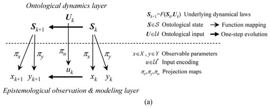
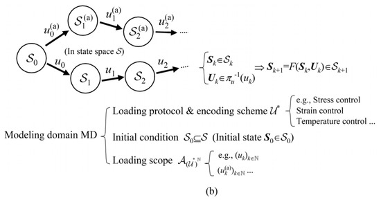
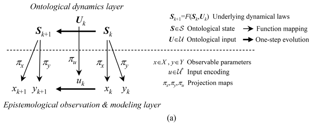
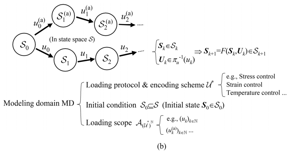
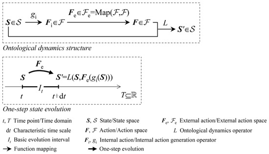
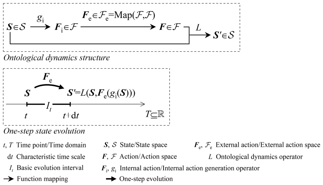
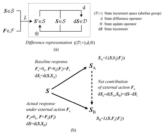
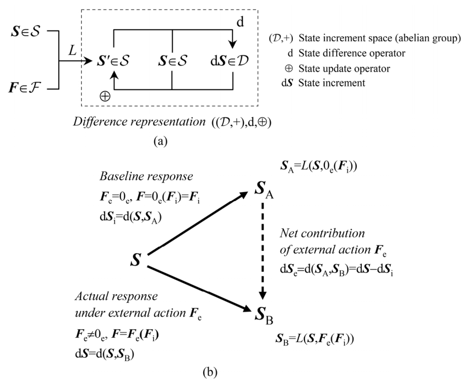
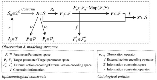
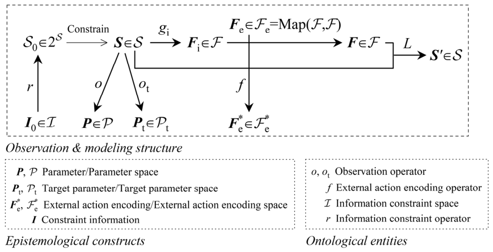
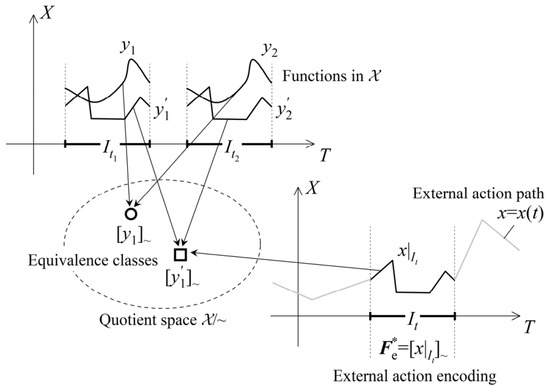
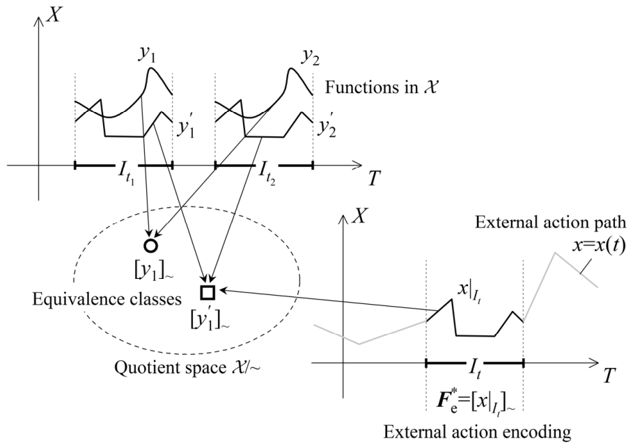
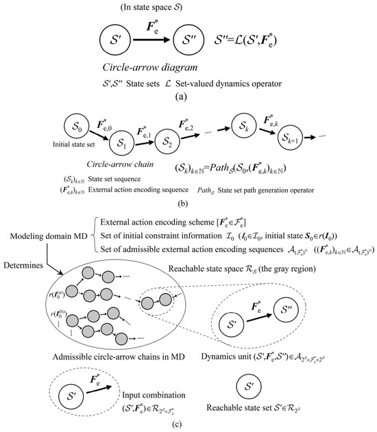
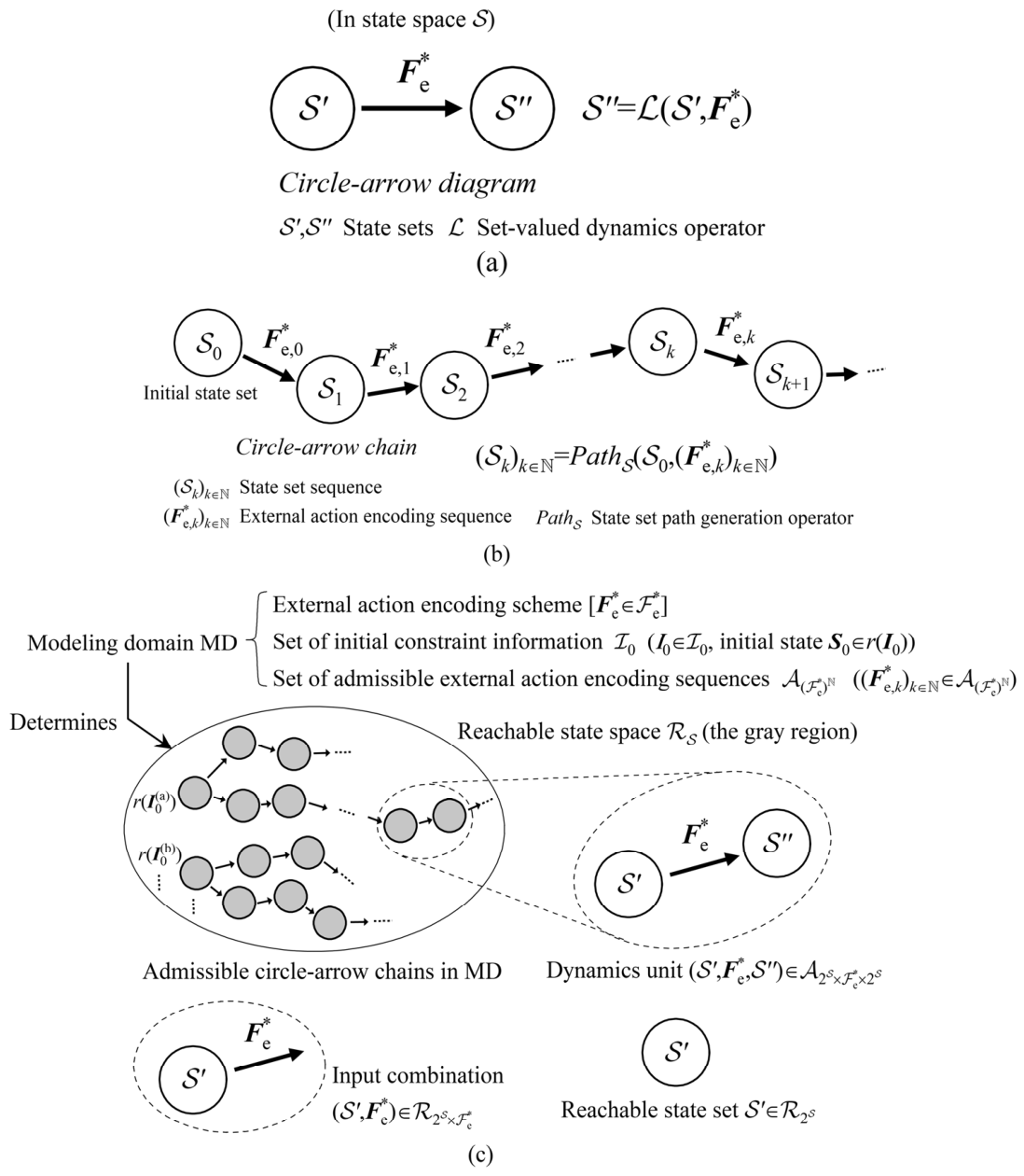
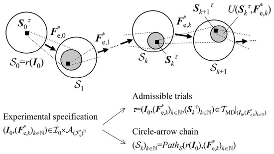
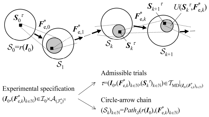
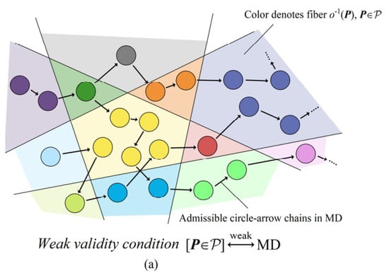
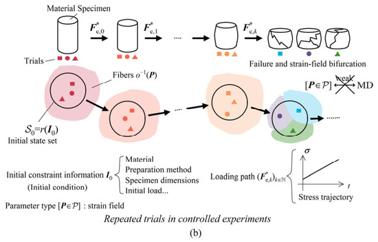
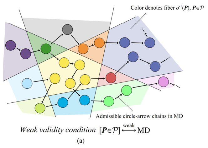
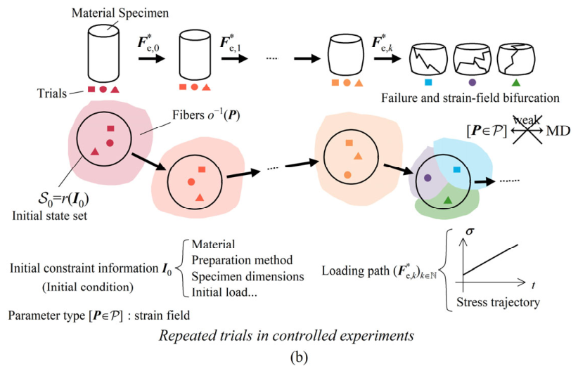
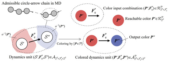
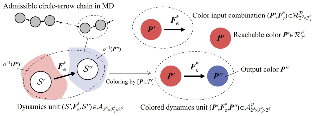
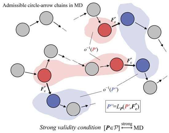
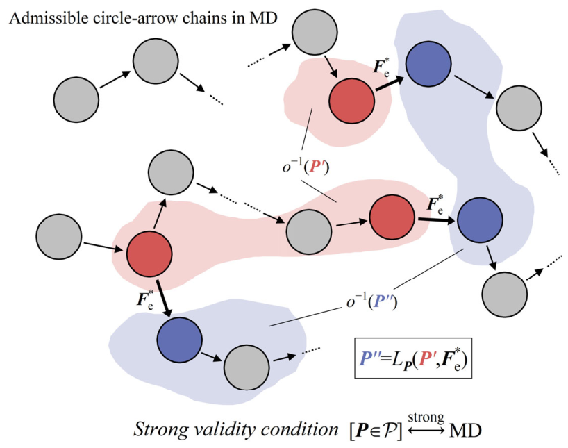
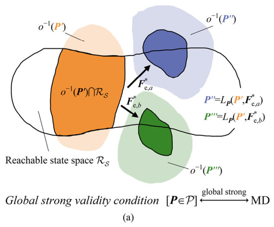
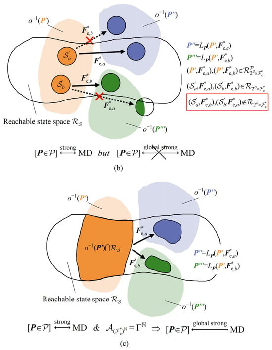
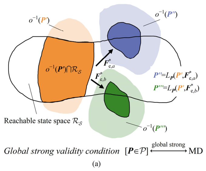
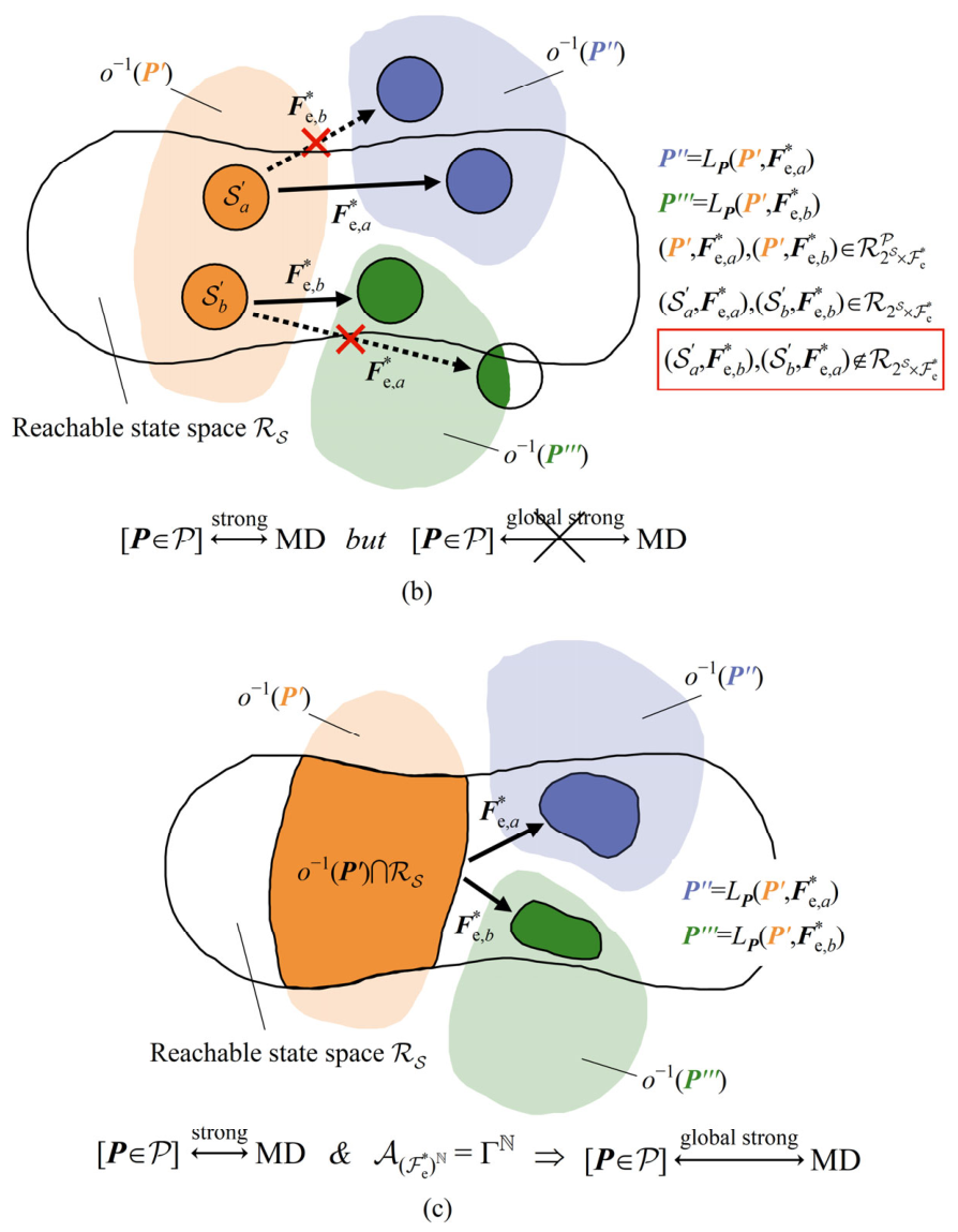
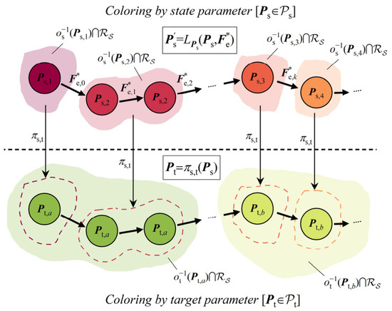
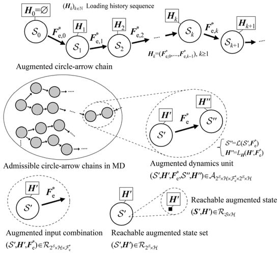
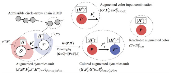
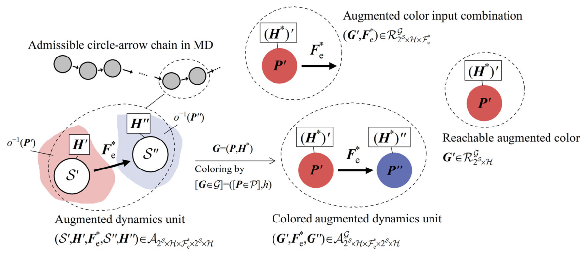
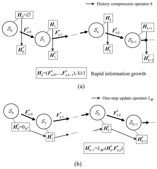
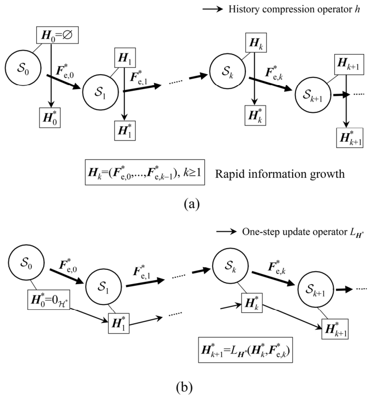
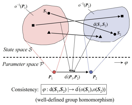
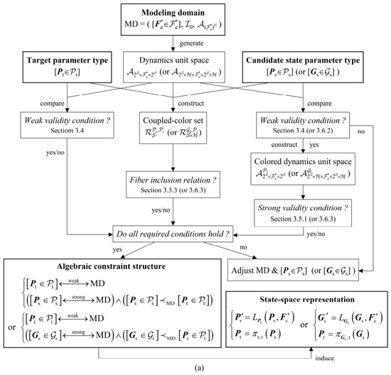
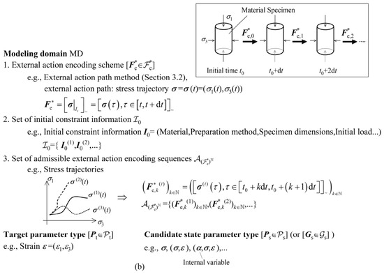
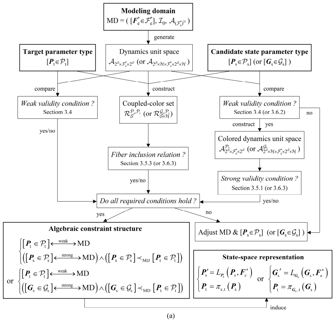
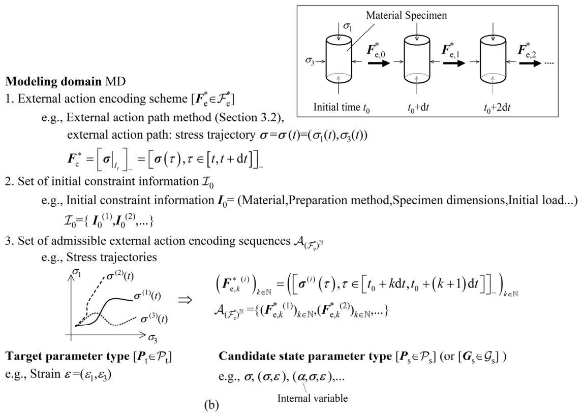
Disclaimer/Publisher’s Note: The statements, opinions and data contained in all publications are solely those of the individual author(s) and contributor(s) and not of MDPI and/or the editor(s). MDPI and/or the editor(s) disclaim responsibility for any injury to people or property resulting from any ideas, methods, instructions or products referred to in the content. |
© 2026 by the authors. Licensee MDPI, Basel, Switzerland. This article is an open access article distributed under the terms and conditions of the Creative Commons Attribution (CC BY) license.