


Abstract
Recent advances in robotics have paved the way for robots to replace humans in perilous situations, such as searching for victims in burning buildings, in earthquake-damaged structures, in uncharted caves, traversing minefields or patrolling crime-ridden streets. These challenges can be generalized as problems where agents have to explore unknown mazes. We propose a cooperative multi-agent system of automated mobile agents for exploring unknown mazes and localizing stationary targets. The Heat Equation-Driven Area Coverage (HEDAC) algorithm for maze exploration employs a potential field to guide the exploration of the maze and integrates cooperative behaviors of the agents such as collision avoidance, coverage coordination, and path planning. In contrast to previous applications for continuous static domains, we adapt the HEDAC method for mazes on expanding rectilinear grids. The proposed algorithm guarantees the exploration of the entire maze and can ensure the avoidance of collisions and deadlocks. Moreover, this is the first application of the HEDAC algorithm to domains that expand over time. To cope with the dynamically changing domain, a red–black successive over-relaxation (SOR) iterative linear solver has been adapted and implemented, which significantly reduced the computational complexity of the presented algorithm when compared to a dense direct solver and to matrix-free BiCGSTAB and GMRES solvers applied to the same linear system. The results highlight significant improvements and show the applicability of the algorithm in different mazes. They confirm its robustness, adaptability, scalability and simplicity, which enables centralized parallel computation to control multiple agents in the maze.
Keywords:
cooperative search; multi-agent system; maze; exploration; graph; successive over-relaxation; frontier-based exploration MSC:
35J05; 65N06; 65D25; 93C85
1. Introduction
Maze exploration has captivated human curiosity over a long period of time. It has served as a valuable tool in scientific investigations, often to assess the cognitive abilities of animals, especially mice, and more recently to study the artificial intelligence of robots. Numerous papers have been published dealing with the exploration of a maze by a single agent or a multi-agent system. To illustrate the long-standing interest of scientists in this topic, it suffices to mention that the Trémaux algorithm dates back to the second half of the 19th century and one of the first papers addressing the maze exploration problem was [1], which investigated the exploration of a two-dimensional maze by one agent (a mechanical mouse) where the agent initially has no knowledge about maze structure. In recent years, increasing attention has been devoted to addressing problems that can be framed as multi-agent maze exploration under challenging conditions, especially in environments with unknown structures. Typical examples include search and rescue missions in burning buildings or locating shipwreck survivors at sea [2], where efficient coordination among multiple agents is critical.
To better understand and solve such problems, various human-centered experiments have been conducted. Their findings offer valuable insights into cognitive processes and can inform the design of intelligent systems inspired by human behavior. For instance, studies [3,4] investigate firefighter wayfinding in complex environments, providing a foundation for the development of real-time multi-agent systems capable of navigating and monitoring such spaces effectively. Recognizing the need for the development of such systems, in this paper we consider the problem of exploring an unknown maze by a cooperative multi-agent system that traverses the maze along continuous paths in discrete time. Each maze is defined by its nodes, which represent possible locations within the maze, and by walls that may separate neighboring nodes. To simulate a real-world application as in [5], collisions, collaboration, coordination of coverage and path planning must be taken into account when controlling the agents. The common goal of maze exploration is to minimize the total time required to find the target or until all nodes are visited (i.e., maze mapping). The maze exploration problem can be divided into two different subtypes: those where the layout of the maze, including the walls and corridors, is already known, and those where it is unknown. Within these subtypes, there are additional variations depending on whether the target location (usually the exit) that agents are looking for in a maze is known, and whether or not these targets are stationary over time. If the layout of the maze is already known, agents usually rely on path planning algorithms to navigate through the maze and eventually reach their target, e.g., an exit. Refs. [6,7] have mentioned some of the known algorithms for single agent maze exploration where the layout of the maze is known in advance, along with the start node and the target node, and of these we will briefly describe some. The dead-end fill algorithm works by tracing the walls of the maze and marking all dead ends or paths that do not lead to the exit. The flood-fill algorithm can also be modified to explore known mazes by assigning a value to each maze node based on its distance to the exit, as described by [7]. Ref. [8] proposed a path planning algorithm based on the “breadth first search” strategy, which is able to identify all possible paths between two maze nodes and select the shortest one. Ref. [9] proposed an algorithm based on a combination of breadth first and depth first algorithms, which proved to be 10–50 times faster than Lee’s algorithm. Ref. [10] introduced another faster variant of Lee’s algorithm, which takes into account the value known as the detour number instead of the distance to the target as a cost measure. Several heuristic search algorithms are also used for this purpose, and one of the best known algorithms of this type is the A* algorithm introduced by [11]. This algorithm combines depth-first search with a heuristic estimate of the cost of reaching the target node. The A* algorithm has been extended to address a wide range of path-planning requirements, including navigation among obstacles in free space [12], robot-size-aware planning that avoids sharp turns [13], planning for self-configurable robots [14], and fuzzy-logic-based variants that adapt to environmental complexity [15]. All the previously mentioned algorithms are primarily intended for single-agent path planning, and according to [16], not many studies have used multi-agent path finding (MAPF) in mazes. One of the other approaches to the problem of path planning and maze exploration is based on the artificial potential field (APF) method, which was originally introduced in [17] with the aim of finding a collision-free path for the robot arm. The basic idea of generating an artificial potential field is to assign an attractive field to the target and a repulsive field to the obstacles in the robot environment. The combination of all repulsive and attractive fields results in the artificial potential field. The robot was considered as a particle that must move in this artificial potential field. The method was subsequently refined and combined into global and local planning schemes [18,19,20], and later extended to near-optimal smooth paths and to dynamic multi-agent target search, for example by combining APF with genetic algorithms to avoid the local-minimum problem [21] or with simulated annealing for teams of multi-link robots [22]. A well-known limitation of APF-based methods is the local-minimum problem, which the method proposed here avoids by construction under the assumptions of Theorem 1.
However, when exploring a known maze, the agent is already familiar with the structure of the maze and enters the maze with a predetermined route to the target. In this way, collisions, dead ends and similar problems that occur when exploring an unknown maze can be avoided. Real-world problems often cannot be reduced to the exploration of a known maze, as we cannot guarantee that the structure we perceive as a maze has not been altered beforehand. For these reasons, we tend to focus on algorithms for exploring unknown mazes. If the structure of the maze is unknown in advance, agents must first explore the immediate environment using sensors and then strategize their actions based on the information gathered. Navigating through an unknown maze in search of stationary goals, such as an exit, therefore involves problems related to detection, search and wayfinding and can be addressed using appropriate methods and techniques. Refs. [6,23] list several basic algorithms for unknown maze exploration by a single agent, where the agent has no prior knowledge about maze structure but knows the starting position: Wall follower, Random Mouse, Tremaux algorithm, Tarry algorithm and Pledge algorithm. The wall follower algorithm is the most commonly used algorithm for exploring mazes. The basic idea is that the agent follows the walls of the maze and applies the right or left rule whenever there is an intersection. This algorithm works well only on perfect mazes. The random mouse algorithm is one of the simplest algorithms for solving mazes. Due to its random movements, the algorithm can take a long time to find the target, especially in large or complex mazes. Tremaux’s algorithm for exploring unknown mazes is one of the first systematic approaches to solving this problem. It is a simple approach to solving mazes based on path markers: The agent traverses the maze and marks each path it traverses; when it encounters an intersection, it chooses an unvisited path or one that has been marked fewer times. This process is repeated until the target in the maze is found. Similar to Tremaux’s algorithm is Tarry’s algorithm, which is based on the idea of constructing a cyclic directed path that traverses each node of the maze once and only once in each direction, and is described in more detail in [23]. Both Tremaux’s algorithm and Tarry’s algorithm are forms of depth-first search (DFS). The basic idea of the Pledge algorithm is that the agent keeps the obstacle on its left or right side while exploring the maze and navigates by summing up the turning angles it encounters along the boundary of the obstacles [24]. Ref. [25] presented a method based on the flood-fill algorithm for exploring an unknown maze by a single agent, where the initial position of the agent and the location of the target are known, but the agent initially has no information about the obstacles between them. Ref. [26] proposed a new method for reducing the travel time through a maze whose wall structure is initially unknown to the micro-mouse robot, and it is based on the Flood-fill algorithm, Bézier curve interpolation, and path tracing techniques. One of the newer path-finding methods that could be used for maze navigation was presented in [27]. This method is primarily intended for pathfinding of robots in unknown environments with unknown target positions and is based on biological firing patterns of cells. This method proved to be fast and memory efficient for uninformed search, e.g., finding the target in a maze. Reinforcement learning (RL) is the process of learning based on a state–reward–action function. One of the best known RL algorithm for path planning is the Q algorithm, which is analyzed in detail in [28]. This approach evolves significantly when integrated with neural networks, leading to the development of the Deep Q-Network (DQN) algorithm, which was used by [29] for the purpose of solving the unknown maze by a single agent. The DQN algorithm uniquely assigns weights based on the results of previous trials, enabling a form of learning that is cumulative and adaptive. In contrast, algorithms such as A* treat all trials performed by the agent with equal importance and focus on predetermined heuristics to guide the search process. This fundamental difference emphasizes the adaptability of the DQN by learning from its environment and making adjusted decisions based on previous experience rather than relying solely on static rules or heuristics. Single-agent maze exploration algorithms are often used to solve mazes, but their extension to multi-agent systems is not optimal and leaves room for improvement.
Cooperative multi-agent exploration of unknown environments has also been extensively studied beyond the maze setting. One of the most established approaches is frontier-based exploration, introduced in [30] and later extended to multi-agent systems in [31]. In this approach, agents are directed toward frontiers, that is, boundaries between explored and unexplored regions. Since several agents may otherwise be attracted to the same frontier, additional coordination mechanisms are commonly introduced. These include centralized cost-utility assignment, where the utility of a frontier is reduced once it has been assigned to an agent [32], as well as market- and auction-based task allocation [33,34].
Another group of methods relies on information-gain criteria rather than geometric frontiers, selecting actions that are expected to reduce uncertainty in the map [35]. More recent approaches combine incremental frontier detection with hierarchical planning to enable efficient exploration of larger environments [36]. When the environment is already known and the main challenge is to resolve conflicts between agents, the problem is usually formulated as multi-agent path finding, where conflict-based search is a widely used optimal approach [37].
Although these methods pursue goals similar to those considered here, they generally rely on different assumptions. They often use metric sensing over multiple cells, a SLAM-based representation of the environment, and an explicit task-assignment or conflict-resolution mechanism. In contrast, the method proposed here is designed for the exploration of an initially unknown maze, assumes a one-node sensing radius, and uses a single scalar field to guide exploration, distribute agents across unexplored regions, and support collision avoidance without requiring a separate task-allocation mechanism. Table 1 summarizes these differences for the approaches most relevant to the present application.
Table 1.
Comparison of cooperative exploration paradigms along the dimensions that are decisive for the present application.
Some of the techniques mentioned were previously used for exploration by a single agent, but their modification allowed them to be used for exploration of the unknown maze by multiple agents. One of these modifications, specifically for the Tarry algorithm, is presented in [38]. The Kivelevitch–Cohen algorithm solves the problem of finding the exit in an unknown perfect maze. It was further modified and improved in [39] for general types of mazes and the implementation of collision avoidance of agents. These two algorithms are explained in more detail in Section 4.2.6. In [40] it is demonstrated how the improved Flood-fill algorithm can be applied to find a target with two agents in a small unknown maze. The effectiveness of the algorithm when using two agents strongly depends on the initial position and orientation of the agents, since the agents can follow the same path, which can reduce the efficiency of the search. Another approach can be found in [41], where a decentralized and asynchronous robot search algorithm based on particle swarm optimization is presented, which is used to solve mazes and find targets in unknown environments. This algorithm proved to be very effective in solving mazes of varying complexity. In [42], it is presented how a bio-inspired technique, specifically ant algorithms (AA), can optimize the search time for a trapped victim in an unknown maze, and then Dijkstra’s algorithm is used for the rescue phase. Four different ant algorithms were implemented to analyze and demonstrate the different effects of pheromones.
It is therefore obvious that multi-agent exploration of unknown mazes represents a very interesting area that is approached with different methods. From Table 1 and Table 2, it is evident that these two areas of research overlap only to a limited extent.
Table 2.
The summary of features of maze exploration algorithms.
Cooperative exploration of unknown environments is a well-developed field, but most existing methods rely on metric maps, sensors that cover multiple cells, and explicit task-allocation or conflict-resolution mechanisms. In contrast, research on maze exploration has largely focused on single-agent methods, while the relatively few multi-agent approaches typically require an additional mechanism for collision avoidance. Therefore, there are still relatively few methods that simultaneously operate in an initially unknown maze, assume a sensing radius of a single node, search for a target at an unknown location, and provide both coverage coordination and collision avoidance through the same field without introducing a separate allocation mechanism. For this reason, we present an algorithm for exploring an unknown maze by multiple agents with the goal of finding a hidden stationary target, e.g., an exit. Each agent explores a part of the maze and immediately communicates information about its current position, recognized walls and visited nodes. The proposed algorithm, hereafter referred to as the HEDAC maze exploration algorithm, is inspired by the HEDAC method presented in [43]. HEDAC is an ergodic multi-agent motion control algorithm that can achieve the given target density of generated agent trajectories. This algorithm has been modified and used in many different applications. The autonomous control for non-uniform spraying of multiple UAVs (unmanned aerial vehicles) presented in [44] has proven that HEDAC-controlled UAV spraying swarms should significantly outperform UAVs operating with other existing path planning methods. A similar task is presented in [45], where a robotic system draws artistic portraits. The control of the drawing is represented as an ergodic coverage problem, which is then solved by a control algorithm based on HEDAC. UAV motion control techniques for search missions [46,47] successfully utilize the HEDAC idea. Static and dynamic obstacle collision avoidance, non-radial sensing capabilities, irregular domains and heterogeneous UAV swarms are the most interesting improvements and extensions of HEDAC in these works. The application of HEDAC to trajectory planning for autonomous three-dimensional visual inspection of infrastructure with multiple UAVs is presented in [48]. The inspection planning method proved to be flexible for different setup parameters and applicable to real inspection tasks. The distributed coverage control of multi-agent systems in uncertain environments using heat transfer equations presented in [49] is also based on HEDAC ideas. More recently, HEDAC was extended to whole-body control of robots equipped with sensors distributed over the body, such as tactile skin [50], and to closed-loop ergodic control on point clouds [51], where the potential field is approximated from transient diffusion by spectral acceleration. The latter work is the closest to the present one in intent, since it also aims at reducing the cost of the repeated field computation, but it operates on a fixed domain. The algorithm presented in this paper is used to control the agents based on a potential field generated by modeling thermal conduction phenomena in a discrete maze. The algorithm provides a built-in cooperative agent behavior that includes collision avoidance, coverage coordination, and near-optimal path planning. In contrast to previous applications of the HEDAC method that investigate a non-variable continuous domain, this work considers a discrete dynamic system in both time and space with a variable spatial domain. In the proposed HEDAC application, the iterative Red-Black Successive Over-Relaxation (RB SOR) method has been used to compute the potential field, which brings a significant performance improvement compared to the techniques used in HEDAC in previous publications (finite difference, finite element and recently published spectral acceleration methods [51]). Since in this work the domain is unknown and dynamically expands as the exploration of the maze progresses, using direct solvers requires not only solving the linear system but also initializing the system at each time step, which is very time consuming, while iterative solvers provide an elegant and effective solution to this problem since the iterations can be easily extended to newly discovered nodes without the need to initialize the linear system. We should also emphasize that algorithms whose goal is to find the target, e.g., an exit, in an unknown maze are not necessarily suitable for visiting all maze nodes, i.e., mapping the entire unknown maze, and vice versa. HEDAC maze exploration algorithm is primarily designed to find a target in an unknown maze, but can also be successfully used to explore the entire unknown maze. Thus, we present not only a new method that represents a novelty in the approach to finding a hidden stationary target in an unknown maze by multiple agents, but also a new application of the HEDAC method that enables successful real-time exploration of an initially unknown and dynamically expanding discrete domain.
The specific contributions of this paper are the following.
- HEDAC is adapted from continuous static domains to an initially unknown, discrete and dynamically expanding rectilinear domain. This is the first application of HEDAC to a domain that grows over time.
- Exploration, coverage coordination and collision avoidance are obtained from a single scalar field, without a separate task-allocation or conflict-resolution layer. The sequential, per-agent updating of the source term is analysed: without collision avoidance it is necessary to prevent the agents from merging, and its effect, together with that of the warm start of the solver, is quantified by an ablation study (Section 4.2.4).
- A matrix-free red–black SOR solver with warm starting and an on-line adaptation of the relaxation parameter is proposed. It removes the need to re-assemble or re-mesh the linear system as the domain grows, and its number of iterations per solve does not grow with the size of the maze in the tested range. It is compared with matrix-free BiCGSTAB and GMRES solvers and with a dense direct solver on the identical linear system with the identical stopping criterion.
- The linear system couples two nodes only through passages that an agent has actually observed (Section Observed Passages), so the potential field uses no information that the agents do not possess.
- Convergence is established analytically. Theorem 1 guarantees complete exploration and the absence of deadlocks.
The basic structure of the paper is as follows. The basic idea of the HEDAC method in 2D continuous space and time domain is described in Section 2. The extension of the original algorithm and problem to the exploration of mazes and the implementation of the HEDAC method in the discrete space and time domain is presented in Section 3. In Section 4.1, the conditions and datasets on which we conducted the numerical tests are described. In Section 4.2, we present the results of all the performed numerical tests. Specifically, we demonstrate the maze exploration process governed by the proposed HEDAC maze exploration algorithm. Additionally, we provide a comparison of the classical direct Gaussian solver and the iterative RB SOR linear solver used in the HEDAC algorithm for maze exploration, as well as with the matrix-free Krylov solvers BiCGSTAB and GMRES. The impact of the collision avoidance mechanism on the test results is also examined. In the same subsection, we compare the HEDAC algorithm for maze exploration with algorithms that have similar goals, presented in [38,39]. Furthermore, in this subsection we analyze the scalability of the HEDAC maze exploration algorithm, followed by the final Section 5, in which the conclusion is presented.
2. The HEDAC Exploration in Two-Dimensional Continuous Domain
The HEDAC method is a centralized control of the motion of agents in the bounded two-dimensional domain with a Lipschitz continuous boundary. In this application, we will allow an expanding space domain such that for . We should emphasize that the domain changes dynamically as the maze is explored/discovered. For now, we consider the trajectories of the mobile agents as known and denote them by , for where N is the number of mobile agents. The coverage function is cumulative and counts how often the location has been visited up to time t. To achieve maximum coverage, the movement of the agent is controlled using a simple first-order kinematic motion model:
with initial conditions
where is the magnitude of the agent velocity and is an attractive scalar field that represents a potential or a temperature and directs the agents via its gradient. It is obtained as a solution of modified Helmholtz equation:
with the Neumann boundary condition
where is a Laplace operator, is outward normal. can be physically interpreted as heat conduction, while , where in (2) represents a convective heat flow and it governs cooling over the entire space domain. With increasing convective cooling, the temperature field u tends to approach the source field, so that more details about the uncovered areas become known. Therefore, an increase in leads to an improvement in local coverage.
The parameter sets the length over which the influence of a source decays: the free-space solution of (2) decays like with the distance r from the source. A small gives a smooth, long-range field that attracts the agents towards the global distribution of the uncovered area, whereas a large gives a localized field in which the agents move greedily towards the nearest uncovered node, which suits a maze, where the geodesic distance between two nodes is often much larger than their Euclidean distance. Very small values of also slow down the iterative solver, because the diagonal dominance of the discrete system decreases with . The agent speed is fixed by the discretization to one node per time step. The source term s is a non-negative spatial field and can be formulated in different ways, for example as in [43,44,46], but for this application it is defined as
which emphasizes the areas insufficiently covered up to time t. The main goal of this method is to control the movement of agents so that the source converges to 0 everywhere, which corresponds to the entire domain being explored, or until the target is found.
3. Formulation of a Discrete Maze Exploration
We consider a simple maze with uniformly wide corridors and simple branches. The maze can be represented as a 2D domain, where the walls of the maze are modeled by Neumann boundary conditions. The maze is initially unknown and may have a hidden target (depending on the problem we want to solve). There are inherent difficulties with variable space domains that make this problem difficult and computationally expensive, such as repeatedly remeshing the numerical domain. We show that we are able to use a multi-agent system driven by a HEDAC-based centralized algorithm to fully map the maze or find the target. However, instead of the real 2D problem presented in Section 2, we solve a simplified version of it, which is obtained by discretization of the space and time domain. This makes the algorithm simple and it is easy to track the dynamic changes in the domain.
3.1. Maze Domain
To simplify the application, we consider only a simple maze with orthogonal corridors in which we can place the nodes of the discrete numerical grid in a 2D coordinate system with integer coordinates. Each node of the numerical grid in Figure 1 represents a position that an agent can occupy. The agent can move orthogonally around a grid node at each time step if the surrounding maze barriers allow this. The distances between neighboring nodes are all the same, so that the agent’s velocity remains constant.
Figure 1.
An example of a maze, represented as a numerical grid: (a) Maze structure. (b) Corresponding numerical grid. Maze walls are represented by a red line, and a possible location in the maze where an agent can stand is represented by black nodes. The edges between these nodes are only used to provide information about whether the two nodes are adjacent or not. A solid black line represents a real connection between two nodes, and a dotted black line represents an obstacle between two nodes.
3.2. Agent Motion Control
Since we focus on the exploration of the maze and the cooperation of the agents, in this paper we use the simplest first-order kinematic model for the agents’ motions, which neglects the mass and inertia of the agents and is constrained to orthogonal motion. We also introduce a new method for collision avoidance when moving through the maze. This algorithm allows agents to stop and wait until another agent is no longer blocking their motion. We have also left the option to allow collisions if an application of the algorithm requires it. At the beginning, the maze is unknown and the main priority of the agent system is to explore the maze. The agents explore the surroundings of their starting position with limited knowledge and focus exclusively on neighboring nodes that are known to them. The agents begin their movement from their starting position and their main goal is to search the unknown maze and find the target. They can only move one step up, down, left or right if there is no wall preventing them from doing so. This means that the directions in (1) are limited to only 4 possibilities, and the agent chooses the one with the greatest potential (which corresponds to the gradient from (1)). The agents cannot go or see through walls, but they can exchange information about their position and the explored parts of the maze. The time domain is discrete . After each time step, the numerical domain and the set of indices are updated with discovered nodes. Therefore, the trajectories of the agents can be described by functions , for . Since the space and time domains are discrete, we can represent the coverage function at time step for the maze node as a cumulative sum of ones and zeros depending on how many times the agents have visited the node up to time step . For each agent that visits the maze node in each time step, 1 is added to the cumulative sum. In this discrete case, the source term s is represented as a non-negative scalar field
which emphasizes the insufficiently covered maze nodes at time step , where is a scaling factor that can be chosen to help the convergence of a linear solver. In our numerical examples, we have used .
Figure 2a, shows an example of a maze node that has no obstacles in the local neighborhood, so that the value of the solution of the PDE Equation (2) can be obtained by discrete finite difference approximation as
because we use we get
Figure 2.
Examples of the maze nodes neighborhood depending on the arrangement of the maze walls: (a) all four neighbors; (b) three neighbors. Maze walls are shown with red lines, while the nodes and the connections between them are shown in black.
It remains to be explained what to do with the more complicated case where an obstacle exists between a node and at least one of its neighboring nodes, as in Figure 2b. Given the structure of the maze shown in Figure 1, we can consider these disconnections/walls between the nodes as boundaries and impose Neumann boundary conditions there, since the Neumann boundary condition actually represents an ideal insulating wall from the point of view of the conductivity model, a barrier in the domain through which no heat is conducted. In the particular case in Figure 2b, we can impose the Neumann boundary condition on the top of the node at position . Second-order approximation of the Neumann boundary condition
where marks a temporary node, modifies the (4) to obtain
There is another interesting case in Figure 2b concerning the node at position , we impose a Neumann boundary condition on the top, bottom and left side of the node. Due to the Neumann boundary condition, the partial derivative vanishes in the vertical direction and the equation reduces to a 1D case:
All cases, including special cases (4)–(6), can be written in a general form that applies to all nodes:
where is set of possible neighbor indices for maze node . The interface function depends on the structure of the walls around the node and applies in general. In the case we are dealing with, where each maze node has at least one neighbor, holds . Equation (7) is valid for nodes with all four neighboring nodes and also in the absence of some neighboring nodes by applying Neumann boundary conditions to the finite difference approximation of the derivatives in (2). The solution of this linear system is a scalar field which is used to control the agents in the maze.
Walls are thus not obstacles inside the domain but parts of its boundary with a homogeneous Neumann condition, and the whole topology of the maze is carried by the interface function . A newly discovered node is only appended to the system with evaluated in its four directions, so no mesh is built or rebuilt. In every row the diagonal entry exceeds the sum of the off-diagonal entries by exactly , which is what makes Theorem 1 hold on every intermediate domain.
Observed Passages
The system describes the maze as it is known to the agents. An agent standing at a node sees which of its four directions are open, so the passage between two adjacent nodes is observed once an agent has stood on one of them. Only then does it enter the system, in the equations of both nodes; until then it is treated as a wall, and when a node is visited for the first time, its row and the rows of its open neighbours are updated. The potential thus uses only information that the agents possess, the diagonal dominance is preserved, and, since every discovered node is coupled to a visited node and consecutive nodes of a trajectory are coupled, the nodes explored by agents whose regions have met form one connected component, as required in Theorem 1. Each agent moves one step at time to a neighboring node where the scalar field u has a larger value. A simple iterative numerical method can be used to approximate the solution by successively averaging over each node:
where r counts the iterations until convergence. Equation (8) describes an iterative Jacobi method. The iterations are very simple and can be performed in parallel using the cumulative computing power of the multi-agent system. Simple iterations allow us to solve a growing domain without re-meshing, as new numerical nodes are simply added to a list and assigned to one of the processors with the lowest load.
Theorem 1.
The iterations defined in (8) converge to a unique solution for an arbitrary initial value u. Furthermore, if the set of discovered nodes at the observed moment forms a single connected component of the maze, and if (the components of s are nonnegative and at least one is nonzero), then and all local maxima of the solution are located at unvisited nodes.
Proof of Theorem 1 .
Equation (8) represents the Jacobi iterative solver for the linear system , which arises from the previously described finite-difference approximation of the problems (2) and (3). Each equation of the linear system is of the form (7), and therefore we can conclude that the system matrix A is strictly diagonally dominant for . From [52] (Theorem 3.4) it follows that the solution is unique and that the Jacobi iterations converge to the unique solution for an arbitrary initial vector u. In general, the system matrix is a strictly diagonally dominant Z-matrix for . If, in addition, the set of discovered nodes at the observed moment forms a single connected component of the maze, then the graph associated with the system matrix is connected, and by [53] (Theorem 2.2.7) matrix A is irreducible. In this case, by [52] (Corollary 3.5.1), we conclude that (all elements of the inverse are strictly positive), and hence if . Now assume that attains a local maximum at some node that was visited before the time step . Then it follows that . Since , from (8) we obtain
which is a contradiction. Therefore, we conclude that a local maximum of can be attained only at an unvisited node. □
Theorem 1 shows that the simple iterations given by Formula (8) always converge and can be used to approximate the values of the potential field u. The agents use the potential field to navigate through the maze according to the principle of steepest ascent: for their new position they always choose a free neighboring node with the highest potential value. A potential deadlock would occur only if an agent were standing at a local maximum. In the proof of Theorem 1 we showed that this is impossible if the set of discovered nodes at the observed moment forms a single connected component of the maze, because a local maximum cannot be attained at a visited node. Since the local maximum is attained at unvisited nodes, the agents move and follow the steepest-ascent hill-climbing algorithm and will continue to do so until they have visited all available nodes. Therefore, Theorem 1 guarantees that the maze will be fully explored if the set of discovered nodes at the observed moment forms a single connected component of the maze. In addition, the iterations are very simple, which simplifies updating the linear system at each time step, making the domain growth problem easy to implement, with very low memory requirements. A drawback of this approach is that the convergence of the Jacobi method slows down on large numerical domains. Convergence can be improved by Gauss–Seidel iterations, where each component of the vector u is computed using the most recently available values of other components from the same iteration. Although the Gauss–Seidel method improves convergence compared to the Jacobi method, its parallelization is not straightforward. In our implementation, with the aim of achieving parallelization and faster convergence of the solution, we used the RB SOR method, which further accelerates the convergence of the Gauss–Seidel method, and whose efficiency depends on the choice of the relaxation parameter . Parallelization of the iterations is achieved by dividing the discovered nodes into two sets using the red–black strategy. We form two sets of nodes, black, , and red, . According to this definition of the sets B and R, the neighbors of any element from the set B are not contained in B but in R, and vice versa. Due to this definition of the sets B and R, the solution by the RB SOR method can be computed in two successive steps:
where r denotes the iteration number. The iterations in steps (9) and (10) are very simple, and each of them can be parallelized.
The efficiency of the RB SOR method depends on the relaxation parameter , whose optimal value is not known a priori for a system that arises on a domain which grows during the computation. The initial value is obtained from formula ([54] Theorem 4), where the spectral radius of the Jacobi iteration matrix is estimated by power iteration on the initial domain. During the exploration, is refined on-line: successive solves are performed in rotation with three candidates, and , and the centre is moved to the candidate with the smallest mean number of iterations, or is halved when the centre itself is the best, so that the adaptation requires no additional solves. Tests of the spectral radius of the SOR iteration matrix for the systems that occurred in the explorations confirmed the convergence for the values of used in all cases. In this approach, neither a global system matrix is assembled nor stored; instead, for each grid node only local data are stored: the diagonal scaling factor and information about neighboring nodes. This enables an efficient and flexible application of the RB SOR method in a dynamically changing domain, with significantly reduced memory requirements and computational time. At each step of the RB SOR iteration, the relative change of the solution is computed for red and black nodes. The iterative procedure is terminated when the maximum relative change becomes smaller than a prescribed tolerance . More precisely, the following criterion is used:
where denotes the change in the potential value at the i-th node, while represents the current solution at that node. If the condition is satisfied or the maximum number of iterations is reached, the procedure is stopped. In all experiments and the maximal number of iterations is 1000; the same criterion, evaluated on two successive iterates, is used for all iterative solvers compared in Section 4.2.2.
Now that we know how u is determined, we can state the rules and the algorithm for controlling the agents’ motion:
- The complete structure of the maze is initially unknown; agents appear at their initial positions and discover only the immediate neighbors of their starting positions. A random node is set as the target/exit of the maze, and the main task of the multi-agent system is to explore the maze and find the target.
- In a single time step, an agent can move only one step up, down, left, or right in the maze.
- In each time step t, an agent can make one move—either move to a neighboring node or remain at the current position.
- The order of movement is defined in advance: the agent with the lowest index decides first on its next position, while the others follow in increasing order.
- Before selecting the next position of an agent, the linear system (9) and (10) is solved with an updated right-hand side (the source term s). In this way, even when the collision-avoidance mechanism is not activated, the occurrence of synchronized agent behavior is avoided, where after occupying the same node they would continue to choose identical subsequent positions and thus effectively act as a single agent.
- The decision on the agent’s next position is based on the values of the potential field u obtained by solving the linear system. If the collision-avoidance mechanism is not active, the next position is chosen as the neighboring node with the highest potential, or the current node if it has the highest potential. If collision avoidance is active, the agent selects the first node with the highest potential among the free neighboring nodes and the current position.
- Information about the selected next position of an agent is immediately shared with the other agents, while data about newly discovered nodes are exchanged among agents only at the end of each time step. In this way, each agent knows which nodes will be occupied and can exclude them from consideration if the collision-avoidance mechanism is active.
- At the end of the time step t, the agents move to their new positions and the data on newly discovered nodes are updated.
- The search ends when one of the agents finds the target/exit of the maze or when the maze is fully explored, i.e., .
The pseudocode of the algorithm is given in Algorithm 1.
| Algorithm 1 Maze exploration with an activated collision-avoidance mechanism |
|
Intuitively, it is clear that the agents, even in situations where the set of discovered nodes in the initial steps does not form a connected component, will eventually discover all nodes of the maze, provided that there exists a path between every pair of nodes in the maze, i.e., that there are no parts of the space inaccessible from their initial positions. Following the previously described procedure, in which they discover all neighboring nodes of their current position and assign a positive source to unvisited nodes, the agents gradually expand the search area until they cover the entire maze. The tests conducted on the sample described in Section 4.1 further confirm that, in practice, the agents fully explore every maze in which all nodes are reachable.
4. Performance Analysis
4.1. Experimental Environment
To properly evaluate the HEDAC maze exploration algorithm, we conducted many maze exploration simulations, varying different exploration methods, maze layouts, the number of agents and their initial positions, and algorithm settings such as anti-collision. In this section, we will describe detailed information about the experimental environment, the datasets used, and the methods used to interpret the results specifically tailored to each test type.
The number of maze exploration simulations performed for each combination of maze configuration, number of agents and algorithm setup is given in Table 3.
Table 3.
Summary of the numbers of simulations of maze exploration. For every maze configuration and number of agents, every layout is explored from 5 random initial configurations of the agents; every HEDAC variant is run with collision avoidance on and off, and the numbers give the runs per collision-avoidance setting. The wall densities and are those of perfect and mazes.
A total of 4 different shapes of mazes were used in the simulations performed, namely , , and , as shown in Table 3. Initially, maze layouts are generated using the backtracking algorithm implemented in the Mazelib (version 0.9.16) Python module (Python 3.12). Each of the generated layouts represents a perfect maze in which any two maze nodes can be connected by a unique path [55]. Exploring a perfect maze is not suitable for evaluation as it only allows limited movement decisions. For this reason, we consider sparser mazes formed by randomly tearing down walls in a perfect maze. We introduce a wall density that represents the fraction of walls present in the maze and the total number of possible walls (if each maze node is completely enclosed by walls). Examples of mazes with different wall densities are shown in Figure 3.
Figure 3.
Examples of mazes with different wall densities: a perfect maze with (a) 49%, (b) 40% and (c) 30%.
For each maze shape, a given number of layouts and initial configurations of the agents are randomly generated. The initial configuration consists of the generated initial positions of the agents, which ensure that there are no overlaps (at most one agent can be located at a node).
Three algorithms for maze exploration are investigated in numerical experiments: Kivelevitch and Cohen, Alian and the proposed HEDAC technique. For HEDAC, four linear solvers are compared on the identical linear system: the matrix-free RB SOR method, the matrix-free Krylov methods BiCGSTAB and restarted GMRES(10) with a Jacobi preconditioner, and the dense direct solver of LAPACK (dgesv). In addition, a dedicated test was performed with HEDAC and RB SOR: the exploration of two fixed mazes, a perfect one and one with wall density, by five agents from 500 random initial configurations (Section 4.2.1). The scalability analysis (Section 4.2.7) uses the runs of Table 3. Moreover, we also investigate different properties of the HEDAC maze algorithm, specifically the motion constraint for collision avoidance and scalability.
All simulations use the same settings for all variants of the HEDAC algorithm: , the second-order treatment of the Neumann condition, the observed-passage rule described in Section Observed Passages, and, for all iterative solvers, the stopping criterion (11) with and a maximum of 1000 iterations per solve. For the first solve, the initial approximation is the zero vector. Each subsequent solve is warm-started using the potential obtained from the preceding solve. For RB SOR, the relaxation parameter is initialized using
and is then adapted online as described in Section 3.2. BiCGSTAB and GMRES are implemented in matrix-free form using the same underlying data as RB SOR, namely the diagonal factors and the lists of neighbouring nodes. Both methods use a Jacobi preconditioner, while GMRES is restarted after 10 inner iterations. For BiCGSTAB and GMRES, the stopping criterion (11) is evaluated from two successive iterates in the same manner as for RB SOR. The direct solver uses the same linear system, but assembles its dense matrix from the same node and neighbour data before each solve. Thus, all solvers operate on the identical system and differ only in the numerical procedure used to obtain its solution. Although we explore all variants to some extent, the SOR solver with collision avoidance mechanism and unknown maze layout is the referent configuration variant of the proposed maze exploration algorithm, that is evaluated in each analysis in the presentation of results.
4.2. Results and Discussion
4.2.1. Maze Explorations Results
We choose a randomly generated layout for a maze to demonstrate exploration by the proposed HEDAC algorithm. The maze is explored by five randomly positioned agents, and all maze nodes are visited after 133 steps (Figure 4). The progress of the exploration can be observed in the trajectories and visible nodes shown in the subfigures (a–c). As more parts of the maze are explored, the more frequently and inevitably existing paths are traversed. This leads to a stagnation of the coverage, as can be seen in Section 4.2.2.
Figure 4.
Example of a simulation of maze exploration by five agents ( wall density). (a), (b) and (c) show agent trajectories and potential in known nodes after 20, 60 and 133 steps, respectively. Grey colored nodes are not known by the algorithm at given step. The values of the potential u range from green (lower values) to light yellow (higher values).
Additionally, we conducted 500 exploration tests on two mazes: one being a perfect maze and the other a more passable maze with a wall density. We prepared a dataset with 500 random initial positions for five agents and tracked the percentage of visited nodes during exploration.
Figure 5 presents the results of those 500 conducted tests, illustrating the differences in exploration efficiency between the two maze types. The perfect maze is explored in steps on average (minimum 28, maximum 123, standard deviation ), the maze with wall density in steps (minimum 26, maximum 53, standard deviation ). It shows that in the first half of the simulation for both mazes the average percent of visited nodes increases almost linearly and the progress slows down in the last half. The results for fewer obstacles are significantly better on average and the variance is obviously lower. This test shows that the exploration of a perfect maze is more sensitive to the initial positions of the agents compared to sparse mazes. This test confirms the intuition that a higher density of obstacles in a maze increases the average number of steps required to explore the maze and increases the sensitivity of the search to the initial positions of the agents.
Figure 5.
Percentage of visited nodes during the exploration of two mazes by five agents from 500 random initial configurations, with collision avoidance and : (a) perfect maze ( wall density), (b) maze with wall density. The dashed vertical line marks the mean number of steps needed to explore the whole maze (the minimum and the maximum are given next to it).
4.2.2. Comparison of Linear Solvers
The linear solver is used to compute the potential field before each agent takes a next step, and this is the bottleneck of the presented algorithm. Therefore, the choice of the linear solver is crucial for the overall complexity of the algorithm. We compare a classical direct Gaussian solver calling a LAPACK routine and the matrix-free Krylov solvers BiCGSTAB and GMRES(10) with the RB SOR method, described by Equations (9) and (10), which is implemented using standard NumPy arrays. Although the RB SOR method is not precompiled, it can exploit the parallelization of NumPy array operations. All four solvers solve the identical linear system from the same warm start and, for the iterative ones, with the same stopping criterion (Section 4.1). Figure 6 shows that the iterative solvers are computationally more efficient than the direct DGESV solver during maze exploration. Since all iterative methods are warm-started from the previous solution, their computational cost remains low and the regression lines slightly decrease as the exploration progresses, while the cost of DGESV increases as the explored domain grows. Among the iterative solvers, RB SOR provides the best performance in this example, typically requiring only a few iterations per solve.
Figure 6.
Example of a simulation of maze exploration with wall density by five agents, on the maze and from the initial positions of Figure 4, with (a) RB SOR (the run shown in Figure 4), (b) BiCGSTAB, (c) GMRES and (d) the direct solver DGESV: CPU time per step, split into the preparation of the linear system, the linear solver (for DGESV including the assembly of the dense matrix before every solve) and the rest of the step, with the linear regression of the solver time (red), percentage of visited nodes, and mean number of iterations per solve. With DGESV the exploration needs one step more, because an exact tie between two candidate nodes is resolved differently.
Figure 7 shows that RB SOR has the lowest computational cost among the iterative solvers in every maze configuration, while the number of exploration steps is practically the same for all solvers. The direct solver is competitive only on the smallest mazes; its cost grows rapidly with the size of the maze, and on mazes it is 170 to 240 times higher than that of RB SOR. The number of RB SOR iterations per solve does not grow with the size of the maze: it is 7–14 on and mazes, 8–10 on and – on mazes.
Figure 7.
Comparison of the linear solvers RB SOR, BiCGSTAB, GMRES and DGESV with collision avoidance: mean CPU time of the preparation and solution of the linear system per exploration, with the minimum and the maximum over the runs (logarithmic axis), and mean number of exploration steps (right).
The iterative solver uses only vector operations, exploits parallelization and has a lower memory load than the direct solver since the linear system is not explicitly constructed. Due to these advantages, the RB SOR solver is used in all the remaining simulations of this section.
4.2.3. Computational Cost per Step
Because the algorithm is intended for the online control of physical agents, the relevant quantity is not only the total computational time but the time consumed by a single exploration step. Table 4 reports the mean, the 99th percentile and the maximum of the CPU time of a complete step, including the update of the system and the solution of the potential for every agent, over all steps of all runs with collision avoidance of each maze size. With RB SOR the mean step takes ms on mazes, ms on mazes and ms on mazes explored by 5 to 20 agents, and no step of any run took longer than 57 ms. The cost of a step grows with the number of agents, since the system is solved once per agent, and with the number of discovered nodes, since one iteration is a pass over these nodes, but not with the number of iterations per solve, which does not grow during the exploration (Figure 6).
Table 4.
CPU time of one complete exploration step, i.e., the update of the system and the solution of the potential for every agent, in milliseconds: mean, 99th percentile and maximum over all steps of all runs with collision avoidance of the given maze size.
RB SOR has the lowest mean and 99th percentile of the step time among the iterative solvers on every maze size. DGESV is the fastest only on mazes; on mazes its mean step takes s and its slowest step s, against ms and 57 ms with RB SOR.
In all 19,000 simulations of the method as proposed (Table 3 and the dedicated test), the coverage reached of the reachable nodes, which is the behaviour predicted by Theorem 1.
4.2.4. Ablation Study
To evaluate the contribution of the two components that characterize the proposed computation of the potential, namely the warm start of the solver and the per-agent update of the field, the reference configuration (RB SOR with collision avoidance) was repeated on all mazes up to and for all numbers of agents listed in Table 3. Two modified configurations were tested: one in which every solve was initialized from (cold start), and one in which the potential was computed only once per time step. In each case, 2200 explorations were performed. Table 5 reports the results for five agents, which is the only configuration used for all three maze sizes; the other numbers of agents lead to the same conclusions.
Table 5.
Ablation study with RB SOR and collision avoidance: mean number of exploration steps, mean solver time per exploration and mean number of iterations per solve, with five agents on every maze configuration (100 explorations on and mazes, 50 on mazes), for the reference method (W: warm start and per-agent update, the runs of the previous sections), the cold start (C) and the update of the field once per time step (O). * Means over the 89 of 100 explorations that were completed with the cold start; the remaining 11 did not finish within 100,000 steps.
With warm start every solve starts from the previous solution of the potential field. Starting every solve from the zero vector instead (cold start) multiplies the solver time by 2.4 to 4.7 without changing the number of steps, and on perfect 20×20 mazes 11 of the 100 explorations did not even finish, because the nodes that the zero initial vector has not yet reached satisfy the relative stopping criterion (11) trivially.
With collision avoidance the potential can also be computed only once per time step instead of once per agent step. Table 5 shows that this reduces the solver time but it also slightly increased the total number of steps. For example, the solver time falls from s to s and the average number of steps rises from to . The per-agent update is nevertheless used as the default, since it is indispensable without collision avoidance. Collision avoidance is not used in applications in which several agents may share a node, for example in the patrolling of streets wide enough for two agents to pass each other.
4.2.5. Collision Avoidance
In the presented algorithm, a linear system is solved and the potential field is updated before each agent chooses the next step. For this reason, it is useful to check the influence of the collision avoidance mechanism. We tested the behavior of the algorithm with AC on and off in perfect mazes and general mazes with 30% wall density. For the tests, we used the dataset described in Section 4.1 and the results of the tests performed can be seen in Figure 8. The Wilcoxon signed-rank test on the paired runs of Figure 9 shows that the difference is small but often statistically significant at . With collision avoidance the exploration needs up to about fewer steps, for example instead of steps on mazes with wall density and 15 agents. Among the configurations with more than one agent, the difference is significant in 11 of 22 cases, and it is never in favour of the exploration without collision avoidance. Another plot of the performance of the HEDAC maze exploration algorithm as a function of the collision avoidance mechanism can be seen in Figure 9. The curves for collision avoidance on and off almost coincide, i.e., the difference, although systematic and in part statistically significant, is small compared with the influence of the maze and of the number of agents. These test results show that the results of the HEDAC algorithm do not require AC on to ensure an efficient workload distribution. If the potential field was updated only once per time step and the agents chose their next step independently, the AC would be necessary to prevent the agents’ paths from merging and traveling together from then on.
Figure 8.
Comparison of the algorithms in terms of the average number of steps required to explore the entire maze: 100 runs per configuration on identical mazes and initial positions; HEDAC with RB SOR with collision avoidance on (plain) and off (hatched), Alian’s algorithm with and Kivelevitch–Cohen’s algorithm without collision avoidance; the ticks mark the minimum and the maximum.
Figure 9.
Influence of collision avoidance mechanism on the performance of the HEDAC maze exploration algorithm: mean number of exploration steps with RB SOR with collision avoidance on and off, for perfect mazes ( and wall density for and , for and ) and sparse mazes with wall density; 100 runs per number of agents on and mazes, 50 on the larger ones.
4.2.6. Comparison with Alternative Algorithms
As can be seen from Table 2 in Section 1, there are not many algorithms that deal with searching in an unknown maze with the goal of finding a target with an unknown location. We have performed two tests in which we compare the HEDAC algorithm with two alternative algorithms presented in [38,39]. We compare the efficiency of the algorithms in terms of the average time steps required for exploring the entire maze, i.e., mapping the entire maze, and the average number of steps required for the first visit to a given node in each scenario. We chose to use the Wilcoxon test to compare both the average number of steps required to explore the maze and the average number of steps required to first visit a particular node in each scenario. This decision was based on the non-parametric nature of the Wilcoxon test, which does not require the assumption of a normal distribution of the data. Given the potential skewness and presence of outliers in the step count data, as well as our sample size, the Wilcoxon test was better suited to accurately assess the central tendencies of our datasets than other statistical tests that assume normality.
Comparison with Kivelevitch and Cohen Algorithm
Kivelevitch and Cohen’s algorithm is used to solve a problem in which a group of agents searches for an exit of the maze (first phase) and, when it has found it, leads the entire group out of the maze through this exit (second phase). In the first phase, i.e., when searching for the exit, each agent follows a generalization of the Tarry algorithm, except that all agents know which node has already been visited. Each agent follows the following rules:
- The agent should move to nodes that have not yet been traveled to by another agent.
- If there are several such nodes, the agent should choose one at random.
- If there is no unvisited node (at least one agent has visited all candidate nodes), the agent should prefer a node that has not yet been visited by it.
- If the agent has already moved in all possible directions or has reached a dead end, it should backtrack to a node that fulfills one of the previous conditions
- All steps should be logged by the agent as it moves.
- When retreating, the nodes from which the agent has retreated should be marked as “dead end”
In order to achieve the completion of the second phase, i.e., to achieve that all agents leave the maze, the Kivelevitch–Cohen algorithm had to ensure that the agents have at least one common point in their paths, which was easiest to achieve by having all agents start from the same position. Since our goal is to find the target, we used only the first phase of Kivelevitch and Cohen’s algorithm to compare with our results, so that it is possible to place the agents in different starting positions. To compare the HEDAC maze exploration algorithm with the algorithm implemented by Kivelevitch and Cohen, we performed tests with 10 × 10 and 20 × 20 perfect mazes as described in Table 3. We used the HEDAC algorithm to explore mazes with the AC off, since Kivelevitch and Cohen’s algorithm works under the same conditions. We tested Kivelevitch and Cohen’s algorithm (using the same data set). As can be seen from Figure 8, the HEDAC algorithm for exploring the maze has no particular advantage over the Kivelevitch and Cohen’s algorithm in terms of the average time steps required to map each node of the maze. According to the Wilcoxon test with a p value of , the differences in the average number of steps required by both algorithms to explore the maze were not significant, except in the case of exploring a 10 × 10 maze with 4 or 5 agents and a 20 × 20 maze with 10 agents, where the average number of steps to explore the maze was lower for the HEDAC maze exploration algorithm. From the results shown in Table 6, it can be seen for how many nodes there is a significant difference in the number of steps required for the first visit, depending on the algorithm used, with a p-value of and it is noted how many of these nodes were visited by the HEDAC maze exploration algorithm in fewer steps on average. Based on these data, it can be concluded that HEDAC performs better compared to Kivelevitch and Cohen’s algorithm when the number of agents is increased. Better performance of the HEDAC algorithm could possibly be achieved by adjusting the parameter, but since we used the settings described in Section 4.1 for all tests, we will not analyze this aspect further here. However, considering that Kivelevitch and Cohen’s algorithm was developed for searching in perfect mazes and cannot be applied to other types, we believe that the roughly equivalent results and adaptability of the HEDAC algorithm for exploring mazes to different maze types provide a sufficient advantage over this algorithm.
Table 6.
Comparison of HEDAC and Kivelevitch–Cohen algorithm on perfect mazes. The total number of nodes with a significantly different average number of time steps for their first visit, and the number of nodes that are, on average, visited earlier by the HEDAC algorithm. .
Comparison with Alian’s Algorithm
The Alian algorithm can be seen as an improvement of the Kivelevitch and Cohen algorithms. It works for all types of mazes and solves the problem of finding the target in the maze and then getting the entire group out of the maze through this exit. In this algorithm, the nodes of the maze are colored in three colors: white are unvisited maze nodes, gray are visited maze nodes, and black are maze nodes from which there is only one path to the exit. When searching for the exit, assuming that an agent detects a neighboring maze node with its sensor, each agent follows the following rules:
- For each currently visited maze node, the occupied flag is set to true so that other agents know that they cannot go there.
- If there is a neighboring maze node that has not yet been visited by an agent (white), the agent should go there. If there are several such nodes, the agent should choose one at random.
- If there is no node that has not yet been visited by an agent, the agent should prefer a gray node that has not yet been visited by it.
- If there are several such nodes, the agent should choose one at random.
- If the agent has already traveled in all possible directions, the agent will choose the gray node it has visited the least time by it.
- If there is only one neighboring maze node that can be visited, but it is currently occupied, the agent should wait at its current maze node until it becomes free
- If there is only one way to leave the current node and all other directions are obstacles or black nodes, the agent marks the current node as a black node so that other agents cannot move there.
A detailed algorithm can be found in [39]. To compare the HEDAC algorithm for maze exploration with the serial implementation of Alian’s algorithm, we performed tests with 10 × 10 and 20 × 20 perfect and more passable mazes as described in Table 3. We use HEDAC with AC on, since the Alian’s algorithm does not impose a collision constraint. From the results shown in Figure 8, it is evident that the HEDAC algorithm requires significantly fewer steps to completely explore sparse mazes with a wall density of , which was also confirmed by conducting a Wilcoxon test with a p-value of . When performing the Wilcoxon test for perfect mazes, we found no significant difference in the exploration results for 10 × 10 mazes with one agent, nor for 20 × 20 mazes explored by one agent, whereas in all other cases, the HEDAC algorithm showed an advantage. We also performed a Wilcoxon test to compare the algorithms based on the average number of time steps required to visit each maze node for the first time, with the results presented in Table 7 and Table 8. In mazes with wall density, the total number of nodes showing a statistically significant difference accounts for 30– of all nodes on and 48– on mazes, and for these nodes, the HEDAC algorithm shows a clear advantage. In perfect mazes, a smaller proportion of nodes shows a significant difference.
Table 7.
Comparison of HEDAC and Alian’s algorithm on perfect mazes. The total number of nodes with a significantly different average number of time steps for their first visit, and the number of nodes that are, on average, visited earlier by the HEDAC algorithm. .
Table 8.
Comparison of HEDAC and Alian’s algorithm on sparse mazes. The total number of nodes with a significantly different average number of time steps for their first visit, and the number of nodes that are, on average, visited earlier by the HEDAC algorithm. .
In perfect mazes, the only case in which Alian’s algorithm visited more of the significantly different nodes earlier is the maze explored by one agent (66 of 128 nodes); in all other cases HEDAC visited the majority of them earlier. However, it is important to note that the total number of nodes with a significant difference is less than half of all nodes.
What is evident is that we have a significant advantage in exploring sparser mazes compared to implementation of the Alian’s algorithm. Additionally, it has been observed that for the Alian algorithm, random bias can significantly influence the total number of steps required to complete the same task.
4.2.7. Scalability
We will discuss scalability in terms of dividing the work between multiple agents, more specifically we will discuss scalability in terms of the percentage of average steps required to explore the maze with a multi-agent system compared to the average steps required to explore the maze with a single agent. In Section 4.2.5 it is shown that the difference caused by collision avoidance is systematic and in part statistically significant at , but small compared with the influence of the maze and of the number of agents, so it is sufficient to analyze the scalability of the HEDAC algorithm with only one of these two options; we use the less favourable one, AC off. Table 9 shows the scalability analysis of the HEDAC maze exploration algorithm in the sparser mazes in terms of speedup coefficient S and efficiency E. The speedup coefficient S stands for the ratio of the average number of time steps an agent needs to explore the entire maze to the average number of time steps n agents need to complete the same task, and the efficiency coefficient E stands for the ratio of speedup to the number of agents. The efficiency coefficient E indicates that although performance increases with additional agents, the improvement is not linear to the number of agents. Consequently, each additional agent reduces efficiency. The efficiency coefficient E, which is relatively high and stable for the results shown in Table 9 for up to 5 agents, indicates that the HEDAC algorithm distributes the tasks quite well among small number of agents. However, the decrease in efficiency when exploring the 20 × 20 maze with 10 agents indicates that the optimal number of agents for 20 × 20 mazes is up to 10.
Table 9.
Scalability of HEDAC algorithm with AC switched off in the unknown maze with 30% obstacles share. Average total number of time steps, speedup coefficient S, and efficiency coefficient E for different numbers of agents used to explore a maze, computed from 100 runs per number of agents (Table 3).
Figure 10 shows an analysis of the average number of steps required to explore different types of mazes with different numbers of agents. This analysis shows that as the number of agents increases, the average number of steps required to explore the maze decreases. However, this reduction deviates further from linearity as the maze structure becomes larger and more complex. From Figure 8 and Figure 10, it can be seen that the HEDAC algorithm also works well for perfect mazes and that the division of labour between agents is good. However, the perfect mazes show a distorted picture of the scalability analysis, which is to be expected since the agents in perfect mazes do not have as many opportunities to choose better paths and overtake each other.
Figure 10.
Analysis of the performance of the HEDAC maze exploration algorithm with various number of agents: mean number of exploration steps with RB SOR and collision avoidance for perfect mazes ( and wall density for and , for and ) and sparse mazes with wall density.
4.2.8. Mapping of a Real Building Floor Plan
Exploring a real building floor plan comes with some additional problems, such as nodes in unreachable areas or holes in the domain. For this example of a realistic application we will show only the HEDAC algorithm result because this type of complex domain is not suitable for other algorithms, which were used for comparison in this paper. Floor plans of the building are shown in Figure 11, where a previously unknown domain is explored using six agents with active collision avoidance mechanism. The HEDAC algorithm successfully maps this complex domain without deadlocks, oscillation or unreasonable changes in direction.
Figure 11.
Real building floor mapping with inactive nodes in white, undetected nodes in gray. Values of the potential u in the image range from green (lower values) to light yellow (higher values).
4.3. Applicability to Real Autonomous Navigation Tasks
Mapping an unknown building, such as the one described in Section 4.2.8, is a practical scenario in which a multi-agent robotic system could save time, reduce resource consumption, and potentially save lives. In a real deployment, the robots would need to construct a map of the environment, solve the associated system of equations, and coordinate their actions while operating under constraints such as limited communication bandwidth and restricted computational resources.
Although the multi-agent system presented in this paper relies on centralized control, the algorithm can be readily adapted to a decentralized architecture. In such a framework, each agent would construct and maintain its own local rectilinear mesh, solve the corresponding linear system using an SOR solver, and exchange information with nearby agents when communication is available. Owing to its simplicity and natural parallelism, the proposed approach is well suited for large teams of robots with modest computational capabilities and limited sensing ranges.
5. Conclusions
The HEDAC maze exploration algorithm proved to be robust, adaptable, scalable and computationally inexpensive. The algorithm does not need to be adapted for each test, except for the parameter , which emphasizes the global or local search of the multi-agent system.
The HEDAC algorithm with the iterative RB SOR linear solver provides a simple and cost-effective solution to the maze exploration problem that can be used in a dynamically changing multi-agent environment and is capable of adapting to various constraints and applications. Moreover, the algorithm does not cause deadlocks and guarantees the exploration of the entire maze if all nodes can be reached. The anti-collision procedure can still be improved, but we have shown that this will certainly not have a major impact on the overall average result. In future work, we will generalize the algorithm to graph search and monitoring, which is an obvious generalization that allows for many different applications. Determining the optimal relaxation parameter in closed form for the non-symmetric system produced by the second-order treatment of the Neumann conditions remains open, and would remove the need for the periodic numerical re-estimation of . In the tested range, up to mazes for all solvers and mazes for RB SOR, the number of RB SOR iterations per solve did not grow with the size of the maze, and the matrix-free BiCGSTAB and GMRES methods with the same warm start and stopping criterion were slower; for considerably larger domains, multigrid or domain-decomposition preconditioning of the same matrix-free operator is the natural next step. The approach taken in this paper can be used to improve similar previous HEDAC implementations in continuous domains as well as on graphs, and also as motivation for exploring new ways to accelerate the HEDAC method.
Author Contributions
B.C.: methodology, conceptualization, supervision, writing—original draft, writing—review and editing, validation, software, formal analysis, investigation. S.I.: methodology, software, writing—review and editing, investigation, supervision, conceptualization, visualization. M.Z.: writing—original draft, writing—review and editing, software, validation, methodology, formal analysis, investigation. All authors have read and agreed to the published version of the manuscript.
Funding
This publication is supported by the European Union—NextGenerationEU—Multi-robot systems for safety operations in unknown environments (uniri-mzi-25-38).
Data Availability Statement
Python code along with maze layouts and agent configurations needed to reproduce this research is publicly available at https://gitlab.com/sivic/hedac-maze-exploration (accessed on 29 September 2026). The entire process of mapping the 40 × 40 maze by 15 agents and the increase in the value of the cumulative function can be viewed on mapping video (https://youtu.be/SWI9Q_tmPC4?si=5ZXN-jvbB8vVzM-w, accessed on 4 December 2023) and cumulative function video (https://youtu.be/9YSC37aZwJs?si=dwYEzYWy9kZcfFNG, accessed on 25 September 2026). Process of mapping 20 × 20 maze by 3 agents where one can track agents trajectories and potential can be viewed on potential tracking video (https://youtu.be/jGd8YDygh7M, accessed on 13 April 2024). Example of exploration of a real building floor plan can be viewed on Real building exploration video (https://youtu.be/R6Hl9F02ZO4, accessed on 13 June 2025). For further inquiries, please contact the corresponding author.
Conflicts of Interest
The authors declare no conflicts of interest. The funders had no role in the design of the study; in the collection, analyses, or interpretation of data; in the writing of the manuscript; or in the decision to publish the results.
References
- Shannon, C.E. Presentation of a Maze-Solving Machine. In Proceedings of the Cybernetics: Transactions of the Eighth Conference; Josiah Macy, Jr. Foundation: New York, NY, USA, 1951; pp. 173–180. [Google Scholar]
- Kou, L.; Gao, X. Advances in Optimized and Safe Path Planning of Marine Autonomous Surface Vehicles: A Review. Sensors 2026, 26, 3445. [Google Scholar] [CrossRef] [Scilit]
- Ye, Y.; Shi, Y.; Xia, P.; Kang, J.; Tyagi, O.; Mehta, R.K.; Du, J. Cognitive Characteristics in Firefighter Wayfinding Tasks: An Eye-Tracking Analysis. Adv. Eng. Inform. 2022, 53, 101668. [Google Scholar] [CrossRef] [Scilit]
- Wang, Y.; Shi, Y.; Du, J.; Lin, Y.; Wang, Q. A CNN-Based Personalized System for Attention Detection in Wayfinding Tasks. Adv. Eng. Inform. 2020, 46, 101180. [Google Scholar] [CrossRef] [Scilit]
- Rahnama, B.; Elci, A.; Ozermen, C. Design and Implementation of Cooperative Labyrinth Discovery Algorithms in Multi-Agent Environment. In Proceedings of the 2013 International Conference on Technological Advances in Electrical, Electronics and Computer Engineering (TAEECE), Konya, Turkey, 9–11 May 2013; pp. 573–578. [Google Scholar] [CrossRef] [Scilit]
- Alamri, S.; Alshehri, S.; Alshehri, W.; Alamri, H.; Alaklabi, A.; Alhmiedat, T. Autonomous Maze Solving Robotics: Algorithms and Systems. Int. J. Mech. Eng. Robot. Res. 2021, 10, 668–675. [Google Scholar]
- Sadik, A.M.J.; Dhali, M.A.; Farid, H.M.A.B.; Rashid, T.U.; Syeed, A. A Comprehensive and Comparative Study of Maze-Solving Techniques by Implementing Graph Theory. In Proceedings of the 2010 International Conference on Artificial Intelligence and Computational Intelligence; IEEE: Piscataway, NJ, USA, 2010; Volume 1, pp. 52–56. [Google Scholar]
- Lee, C.Y. An Algorithm for Path Connections and Its Applications. IRE Trans. Electron. Comput. 1961, EC-10, 346–365. [Google Scholar] [CrossRef] [Scilit]
- Soukup, J. Fast Maze Router. In Proceedings of the Design Automation Conference, Las Vegas, NV, USA, 19–21 June 1978; pp. 100–102. [Google Scholar]
- Hadlock, F.O. A Shortest Path Algorithm for Grid Graphs. Networks 1977, 7, 323–334. [Google Scholar] [CrossRef] [Scilit]
- Hart, P.E.; Nilsson, N.J.; Raphael, B. A Formal Basis for the Heuristic Determination of Minimum Cost Paths. IEEE Trans. Syst. Sci. Cybern. 1968, 4, 100–107. [Google Scholar] [CrossRef] [Scilit]
- Warren, C.W. Fast Path Planning Using Modified A* Method. In Proceedings of the IEEE International Conference on Robotics and Automation; IEEE: Piscataway, NJ, USA, 1993; pp. 662–667. [Google Scholar]
- ElHalawany, B.; Abdel-Kader, H.; Tag Eldien, A.; Elsayed, A.; Nossair, Z. Modified A* Algorithm for Safer Mobile Robot Navigation. In Proceedings of the International Conference on Modelling, Identification and Control (ICMIC), Cairo, Egypt, 31 August–2 September 2013; pp. 74–78. [Google Scholar]
- Le, A.V.; Prabakaran, V.; Sivanantham, V.; Mohan, R.E. Modified A-Star Algorithm for Efficient Coverage Path Planning in Tetris Inspired Self-Reconfigurable Robot with Integrated Laser Sensor. Sensors 2018, 18, 2585. [Google Scholar] [CrossRef] [Scilit]
- Airlangga, G. Fuzzy A* for Optimum Path Planning in a Large Maze. Bul. Ilm. Sarj. Tek. Elektro 2023, 5, 455–466. [Google Scholar] [CrossRef] [Scilit]
- Tjiharjadi, S.; Razali, S.; Sulaiman, H.A. A Systematic Literature Review of Multi-Agent Pathfinding for Maze Research. J. Adv. Inf. Technol. 2022, 13, 358–367. [Google Scholar] [CrossRef] [Scilit]
- Khatib, O. Real-Time Obstacle Avoidance for Manipulators and Mobile Robots. Int. J. Robot. Res. 1986, 5, 90–98. [Google Scholar] [CrossRef] [Scilit]
- Krogh, B.H. A Generalized Potential Field Approach to Obstacle Avoidance Control. In Proceedings of the SME Conference on Robotics Research: The Next Five Years and Beyond, Bethlehem, PA, USA, 14–16 August 1984; pp. 11–22. [Google Scholar]
- Thorpe, C.E. Path Relaxation: Path Planning for a Mobile Robot. In Proceedings of the AAAI Conference on Artificial Intelligence, Austin, TX, USA, 6–10 August 1984; pp. 318–321. [Google Scholar]
- Krogh, B.H.; Thorpe, C.E. Integrated Path Planning and Dynamic Steering Control for Autonomous Vehicles. In Proceedings of the 1986 IEEE International Conference on Robotics and Automation; IEEE: Piscataway, NJ, USA, 1986; pp. 1664–1669. [Google Scholar]
- Vadakkepat, P.; Tan, K.C.; Wang, M.L. Evolutionary Artificial Potential Fields and Their Application in Real-Time Robot Path Planning. In Proceedings of the 2000 Congress on Evolutionary Computation (CEC 2000); IEEE: Piscataway, NJ, USA, 2000; Volume 1, pp. 256–263. [Google Scholar]
- Yagnik, D.; Ren, J.; Liscano, R. Motion Planning for Multi-Link Robots Using Artificial Potential Fields and Modified Simulated Annealing. In Proceedings of the 2010 IEEE/ASME International Conference on Mechatronic and Embedded Systems and Applications; IEEE: Piscataway, NJ, USA, 2010; pp. 421–427. [Google Scholar]
- Rao, N.S.V.; Kareti, S.; Shi, W.; Iyengar, S.S. Robot Navigation in Unknown Terrains: Introductory Survey of Non-Heuristic Algorithms; Technical Report; Oak Ridge National Laboratory: Oak Ridge, TN, USA, 1993. [Google Scholar] [CrossRef] [Scilit]
- Abelson, H.; diSessa, A.A. Turtle Geometry: The Computer as a Medium for Exploring Mathematics; MIT Press: Cambridge, MA, USA, 1980. [Google Scholar]
- Elshamarka, I.; Saman, A. Design and Implementation of a Robot for Maze-Solving Using Flood-Fill Algorithm. Int. J. Comput. Appl. 2012, 56, 8–13. [Google Scholar] [CrossRef] [Scilit]
- Rathnayake, O.; Wijesekara, G.; Samaranayake, L. A Path Planning Technique to Reduce the Travel Time of a Micromouse. In Proceedings of the 2023 IEEE 17th International Conference on Industrial and Information Systems (ICIIS), Peradeniya, Sri Lanka, 25–26 August 2023; pp. 519–523. [Google Scholar]
- Naghizadeh, A.; Berenjian, S.; Margolis, D.J.; Metaxas, D.N. GNM: GridCell Navigational Model. Expert Syst. Appl. 2020, 148, 113217. [Google Scholar] [CrossRef] [Scilit]
- Jang, B.; Kim, M.; Harerimana, G.; Kim, J.W. Q-Learning Algorithms: A Comprehensive Classification and Applications. IEEE Access 2019, 7, 133653–133667. [Google Scholar] [CrossRef] [Scilit]
- Nandy, A.; Seshathri, S.; Sarkar, A. Maze Solving Using Deep Q-Network. In Proceedings of the 2023 6th International Conference on Advances in Robotics, New York, NY, USA, 5–8 July 2023. [Google Scholar]
- Yamauchi, B. A Frontier-Based Approach for Autonomous Exploration. In Proceedings of the 1997 IEEE International Symposium on Computational Intelligence in Robotics and Automation (CIRA’97), Monterey, CA, USA, 10–11 July 1997; pp. 146–151. [Google Scholar] [CrossRef] [Scilit]
- Yamauchi, B. Frontier-Based Exploration Using Multiple Robots. In Proceedings of the Second International Conference on Autonomous Agents (AGENTS ’98), Minneapolis, MN, USA, 9–13 May 1998; pp. 47–53. [Google Scholar] [CrossRef] [Scilit]
- Burgard, W.; Moors, M.; Stachniss, C.; Schneider, F.E. Coordinated Multi-Robot Exploration. IEEE Trans. Robot. 2005, 21, 376–386. [Google Scholar] [CrossRef] [Scilit]
- Gerkey, B.P.; Matarić, M.J. A Formal Analysis and Taxonomy of Task Allocation in Multi-Robot Systems. Int. J. Robot. Res. 2004, 23, 939–954. [Google Scholar] [CrossRef] [Scilit]
- Korsah, G.A.; Stentz, A.; Dias, M.B. A Comprehensive Taxonomy for Multi-Robot Task Allocation. Int. J. Robot. Res. 2013, 32, 1495–1512. [Google Scholar] [CrossRef] [Scilit]
- Stachniss, C.; Grisetti, G.; Burgard, W. Information Gain-Based Exploration Using Rao-Blackwellized Particle Filters. In Proceedings of the Robotics: Science and Systems I, Cambridge, MA, USA, 8–11 June 2005; pp. 65–72. [Google Scholar] [CrossRef] [Scilit]
- Zhou, B.; Zhang, Y.; Chen, X.; Shen, S. FUEL: Fast UAV Exploration Using Incremental Frontier Structure and Hierarchical Planning. IEEE Robot. Autom. Lett. 2021, 6, 779–786. [Google Scholar] [CrossRef] [Scilit]
- Sharon, G.; Stern, R.; Felner, A.; Sturtevant, N.R. Conflict-Based Search for Optimal Multi-Agent Pathfinding. Artif. Intell. 2015, 219, 40–66. [Google Scholar] [CrossRef] [Scilit]
- Kivelevitch, E.H.; Cohen, K. Multi-Agent Maze Exploration. J. Aerosp. Comput. Inf. Commun. 2010, 7, 391–405. [Google Scholar] [CrossRef] [Scilit]
- Alian, H. Multi-Agent Asynchronous Real-Time Maze-Solving. Ph.D. Thesis, University of Alberta, Edmonton, AB, Canada, 2022. [Google Scholar]
- Tjiharjadi, S.; Razali, S.; Sulaiman, H.A.; Fernando, G. Design of Multi-Agent Pathfinding Robot Using Improved Flood Fill Algorithm in Maze Exploration. Int. J. Mech. Eng. Robot. Res. 2022, 11, 631–638. [Google Scholar] [CrossRef] [Scilit]
- Youssefi, K.A.R.; Rouhani, M. Swarm Intelligence Based Robotic Search in Unknown Maze-Like Environments. Expert Syst. Appl. 2021, 178, 114907. [Google Scholar] [CrossRef] [Scilit]
- Husain, Z.; Al Zaabi, A.; Hildmann, H.; Saffre, F.; Ruta, D.; Isakovic, A.F. Search and Rescue in a Maze-Like Environment with Ant and Dijkstra Algorithms. Drones 2022, 6, 273. [Google Scholar] [CrossRef] [Scilit]
- Ivić, S.; Crnković, B.; Mezić, I. Ergodicity-Based Cooperative Multiagent Area Coverage via a Potential Field. IEEE Trans. Cybern. 2016, 47, 1983–1993. [Google Scholar] [CrossRef] [Scilit]
- Ivić, S.; Andrejčuk, A.; Družeta, S. Autonomous Control for Multi-Agent Non-Uniform Spraying. Appl. Soft Comput. 2019, 80, 742–760. [Google Scholar] [CrossRef] [Scilit]
- Löw, T.; Maceiras, J.; Calinon, S. drozBot: Using Ergodic Control to Draw Portraits. IEEE Robot. Autom. Lett. 2022, 7, 11728–11734. [Google Scholar] [CrossRef] [Scilit]
- Ivić, S. Motion Control for Autonomous Heterogeneous Multiagent Area Search in Uncertain Conditions. IEEE Trans. Cybern. 2020, 52, 3123–3135. [Google Scholar] [CrossRef] [Scilit]
- Ivić, S.; Sikirica, A.; Crnković, B. Constrained Multi-Agent Ergodic Area Surveying Control Based on Finite Element Approximation of the Potential Field. Eng. Appl. Artif. Intell. 2022, 116, 105441. [Google Scholar] [CrossRef] [Scilit]
- Ivić, S.; Crnković, B.; Grbčić, L.; Matleković, L. Multi-UAV Trajectory Planning for 3D Visual Inspection of Complex Structures. Autom. Constr. 2023, 147, 104709. [Google Scholar] [CrossRef] [Scilit]
- Zheng, Y.; Zhai, C. Distributed Coverage Control of Multi-Agent Systems in Uncertain Environments Using Heat Transfer Equations. arXiv 2022, arXiv:2204.09289. [Google Scholar]
- Bilaloglu, C.; Löw, T.; Calinon, S. Whole-Body Exploration with a Manipulator Using Heat Equation. arXiv 2023, arXiv:2306.16898. [Google Scholar]
- Bilaloglu, C.; Löw, T.; Calinon, S. Tactile Ergodic Control Using Diffusion and Geometric Algebra. arXiv 2024, arXiv:2402.04862. [Google Scholar]
- Varga, R.S. Matrix Iterative Analysis; Prentice Hall: Englewood Cliffs, NJ, USA, 1962. [Google Scholar]
- Berman, A.; Plemmons, R.J. Nonnegative Matrices in the Mathematical Sciences; Classics in Applied Mathematics; Society for Industrial and Applied Mathematics: Philadelphia, PA, USA, 1994; Volume 9. [Google Scholar]
- Yang, S.; Gobbert, M.K. The Optimal Relaxation Parameter for the SOR Method Applied to a Classical Model Problem; Technical Report number TR2007-6; University of Maryland: Baltimore, MD, USA, 2007. [Google Scholar]
- Bellot, V.; Cautrès, M.; Favreau, J.M.; Gonzalez-Thauvin, M.; Lafourcade, P.; Le Cornec, K.; Mosnier, B.; Rivière-Wekstein, S. How to Generate Perfect Mazes? Inf. Sci. 2021, 572, 444–459. [Google Scholar] [CrossRef] [Scilit]
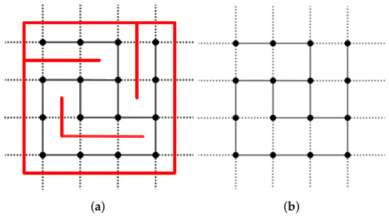
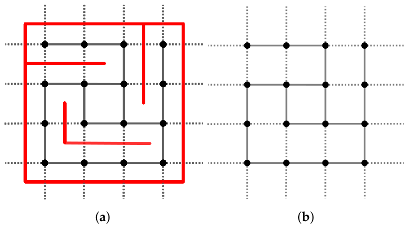
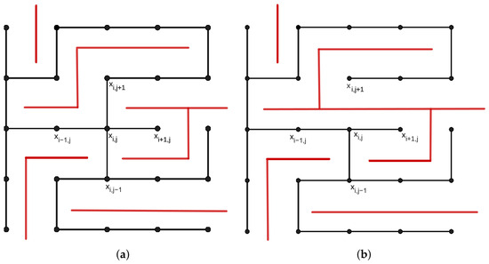
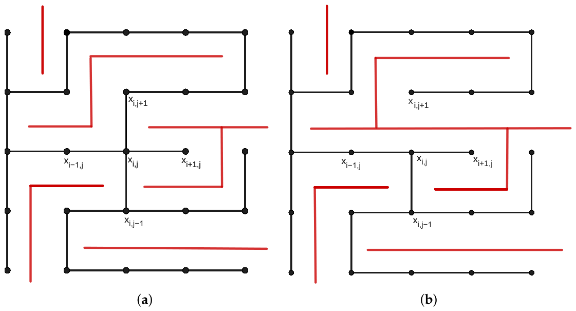
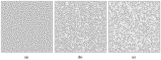
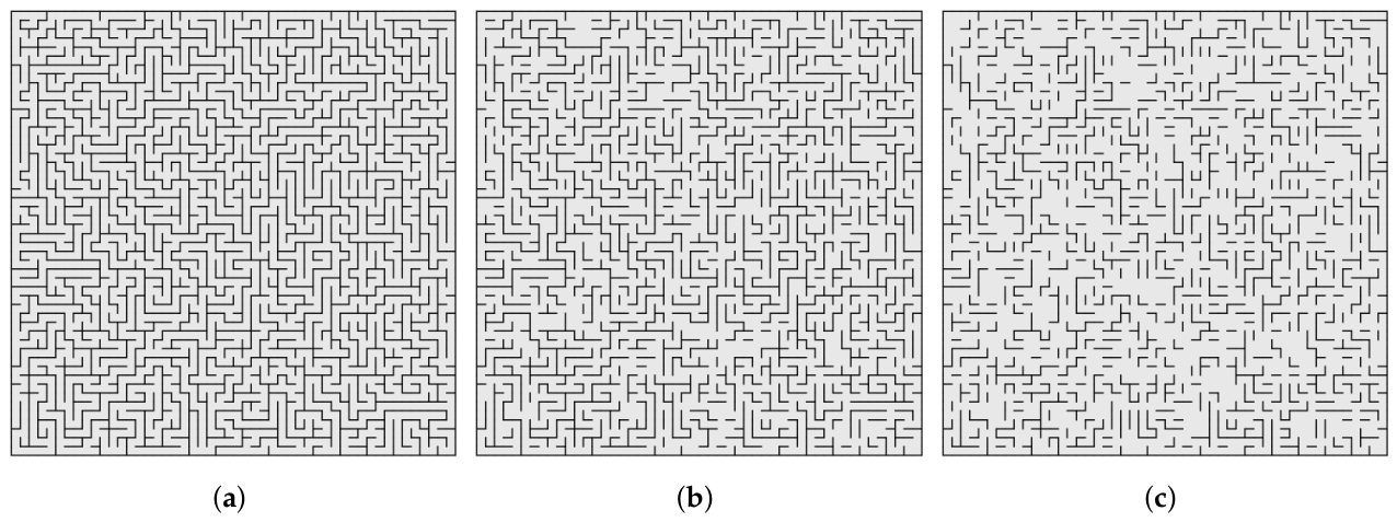
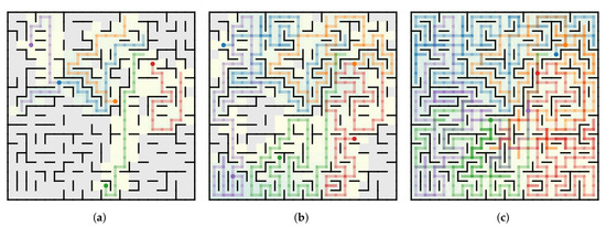
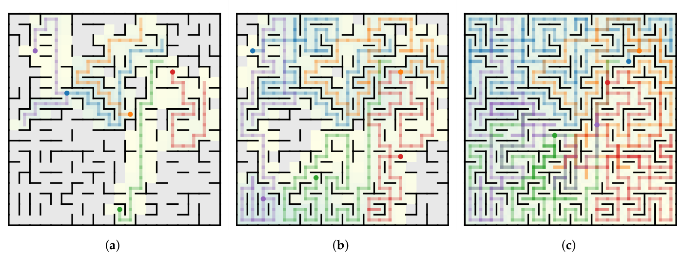
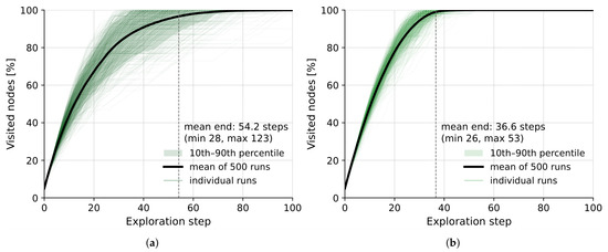
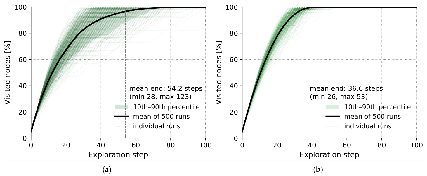
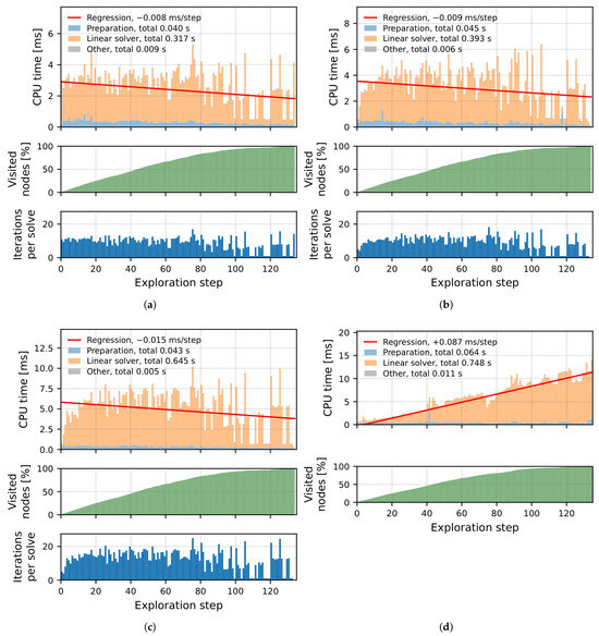
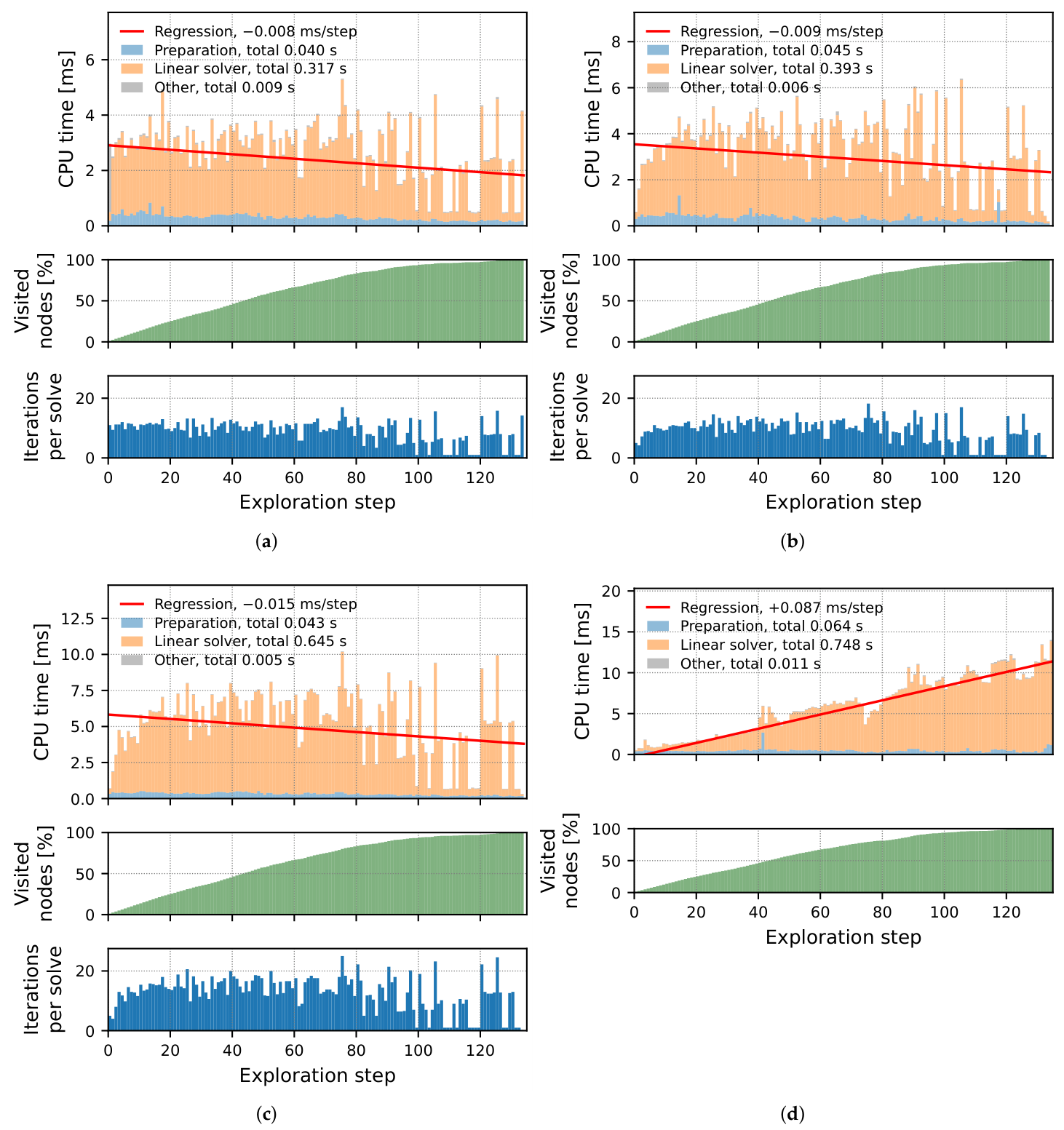
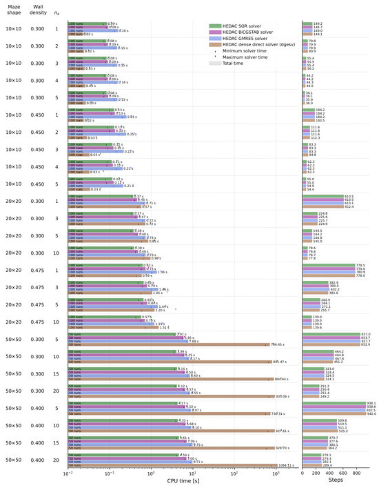
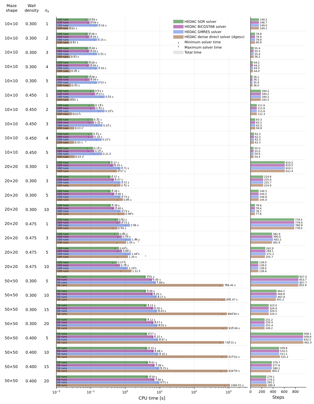
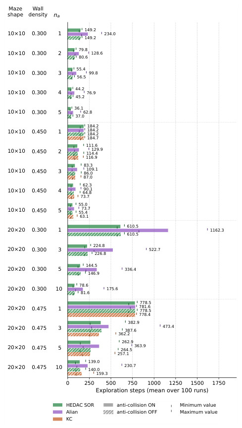
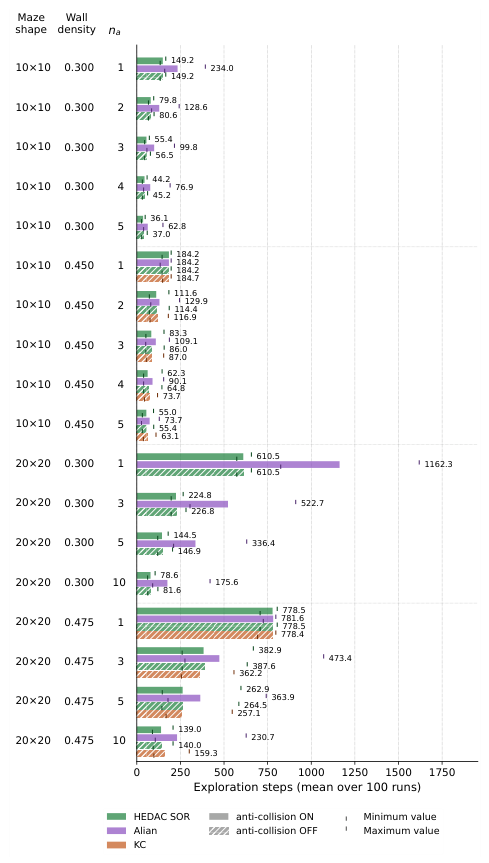
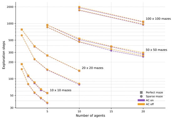
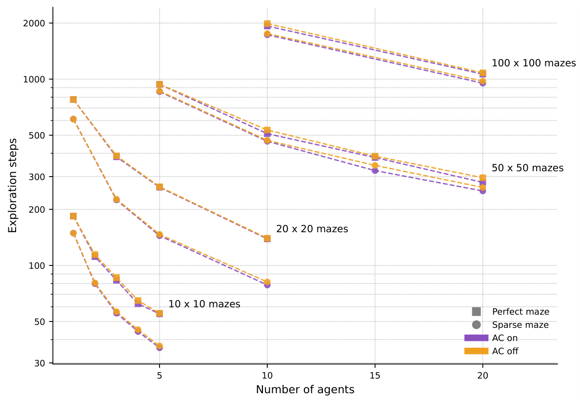
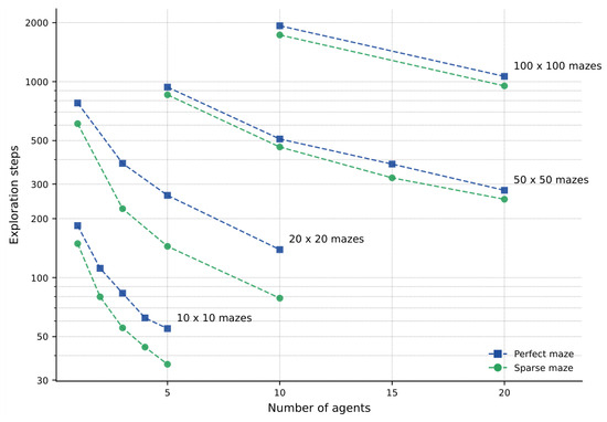
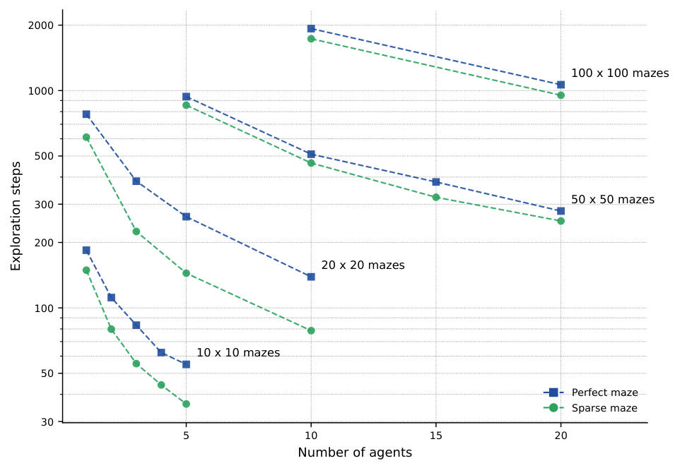
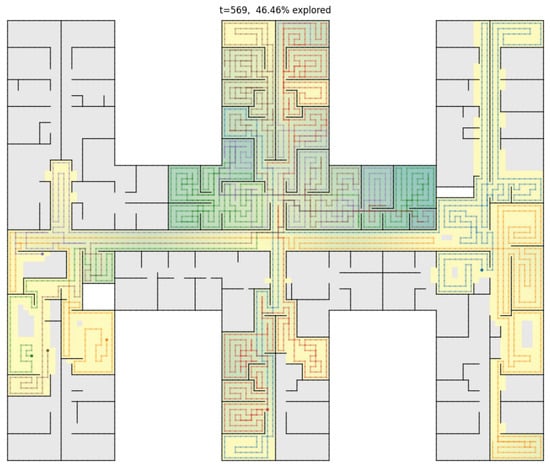
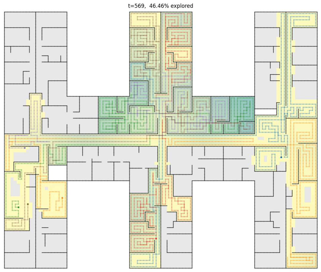

Disclaimer/Publisher’s Note: The statements, opinions and data contained in all publications are solely those of the individual author(s) and contributor(s) and not of MDPI and/or the editor(s). MDPI and/or the editor(s) disclaim responsibility for any injury to people or property resulting from any ideas, methods, instructions or products referred to in the content. |
© 2026 by the authors. Licensee MDPI, Basel, Switzerland. This article is an open access article distributed under the terms and conditions of the Creative Commons Attribution (CC BY) license.