


Abstract
Sparse time-indexed transaction data create a statistical-learning problem in which low basket occupancy, combinatorial candidate growth, temporal heterogeneity, and data-quality sensitivity complicate interpretable pattern discovery. Using a multi-year single-case dataset from an independently operated SME restaurant point-of-sale (POS) system, this study proposes a reproducible, sparsity-aware framework that separates global distributional characterization, unsupervised co-occurrence learning, statistical qualification, adjusted outcome modeling, and transparent prioritization. The empirical application comprises 31,157 baskets, 139,396 valid item lines, 710 products, and 762 active days; the 31,157 × 710 basket-product representation has 0.630% density. Multiplicity-screened association-rule learning retains 1174 directional rules. In a strictly subsequent validation period, 93.6% of discovery rules preserve lift above one, 49.3% satisfy all prespecified thresholds again, and rank correlations for support, confidence, and lift range from 0.803 to 0.849. An estimated-dispersion NB2 model with day-clustered uncertainty preserves the principal basket-breadth associations, while Gamma sensitivity analysis confirms the direction, but not invariant magnitude, of late-service basket-value effects. The methodological contribution is not a new stand-alone algorithm, but an auditable evidence architecture that explicitly separates candidate discovery, multiplicity screening, effect assessment, temporal replication, adjusted modeling, and human-supervised prioritization. Because the empirical evaluation is based on a single time-indexed case, the reported effect magnitudes remain case-specific.
Keywords:
statistical learning; association-rule mining; sparse transaction data; multiple testing; temporal validation; Shannon entropy; negative binomial regression; Gamma regression; reproducible analytics MSC:
62R07; 62J12; 62J15; 68T09; 94A17
1. Introduction
High-granularity transaction records create a statistical-learning problem that is not adequately described by record count alone. In sparse basket data, a large product universe coexists with low within-basket occupancy, repeated temporal contexts, data-quality sensitivity, and a combinatorial candidate space. The central methodological task is therefore to construct an analytical representation that is computationally tractable, statistically qualified, interpretable, and reproducible rather than to maximize predictive complexity. Contemporary work on machine learning for large data likewise emphasizes that dimensionality, variety, veracity, and computational structure jointly determine analytical difficulty [1].
The framework developed here treats unsupervised pattern discovery and statistical inference as different evidential layers. Association-rule learning identifies local co-occurrence structure in an inspectable antecedent-consequent form; normalized Shannon entropy characterizes global concentration and dispersion; and generalized linear models quantify adjusted associations for basket-level outcomes under explicit distributional assumptions. None of these layers is interpreted as causal, and no algorithmic rule is treated as operationally important solely because it is detectable in a large sample.
Restaurant point-of-sale (POS) records provide a demanding real-world test case because they combine repeated transactions, high item sparsity, strongly skewed monetary outcomes, temporal heterogeneity, and recurrent product co-occurrence. Restaurant analytics has addressed revenue management, forecasting, consumer behavior, and recommendation-oriented applications [2], while longitudinal data-mining studies demonstrate the value of interpretable pattern extraction from repeated observational records [3]. The restaurant setting is therefore used as an empirical validation environment for a more general methodological problem: statistically qualifying interpretable structure discovered in sparse time-indexed transaction data.
This study is positioned within the convergence of statistical modeling, unsupervised machine learning, and data-mining practice. Recent contributions in Mathematics show the value of multi-stage frameworks that combine machine-learning representations with probabilistic, statistical, or econometric models [4,5]. The present framework extends this logic to sparse co-occurrence data by making candidate-space reduction, pair-level multiplicity screening, strictly subsequent temporal replication, adjusted outcome modeling, and transparent rule prioritization explicit stages of one reproducible evidence pipeline.
The empirical implementation covers 20 May 2024 to 28 June 2026 and contains 31,157 reconstructed baskets and 710 products. The corresponding binary basket-product representation contains 22,121,470 potential positions but only 139,394 observed product presences, while the unconstrained unordered pair universe contains 251,695 product pairs. These quantities motivate an explicitly sparse formulation and a candidate-reduction strategy. The analysis does not claim streaming performance, distributed-system scalability, causal identification, or population-level generalization beyond the observed case.
The contribution is threefold. First, this study specifies a sparsity-aware statistical-learning architecture in which deterministic data validation, basket reconstruction, global entropy, and interpretable association-rule discovery are linked without conflating their inferential roles. Second, it qualifies a large family of co-occurrence patterns through pair-level multiplicity screening, effect-size information, threshold sensitivity, and strictly subsequent temporal validation, thereby separating in-sample detection from temporal persistence. Third, it integrates adjusted Negative Binomial and Gamma modeling with a transparent, sensitivity-tested rule-prioritization layer, while preserving explicit boundaries between descriptive pattern discovery, statistical association, and human-supervised decision use. Reproducibility and publication-safe data governance operate across all three contributions. The novelty lies in the formally ordered qualification of evidence across these stages, rather than in presenting any established component as a new stand-alone algorithm.
The empirical analysis is organized around four research questions:
- RQ1.
- How do normalized entropy and basket-level composition characterize global demand dispersion across temporal contexts in sparse time-indexed transaction data?
- RQ2.
- Which co-occurrence patterns survive multiplicity screening and retain positive association strength, relative ranking, and threshold robustness in a strictly subsequent validation period?
- RQ3.
- How are observed temporal contexts associated with basket breadth and basket value after adjustment for calendar month and year?
- RQ4.
- How stable is transparent multi-criteria rule prioritization under the ranking-equivalent empirical score and alternative weighting schemes?
2. Literature Review
2.1. Statistical Learning for Sparse Transaction Data, Data Quality, and Representation
Statistical and machine-learning validity depends not only on the choice of algorithm but also on the quality and representation of the data presented to that algorithm. Empirical evidence across classification, regression, and clustering tasks shows that accuracy, completeness, consistency, and other data-quality dimensions can materially alter model performance [6]. Contemporary tooling therefore incorporates data-quality assessment, leakage detection, feature screening, and preprocessing into the analytical lifecycle rather than treating them as invisible preparatory operations [7]. The present workflow adopts the same principle for transaction data by making deletion filtering, identifier validation, relational reconstruction, duplicate control, and arithmetic consistency auditable components of the method.
The source architecture separates transaction headers from item lines, while the analytical problem requires stable observational units. Reconstructing a basket therefore entails a sequence of deterministic transformations: logical-deletion filtering, transaction validation, key assessment, relational linkage, item-line validation, duplicate detection, and arithmetic reconciliation. This sequence establishes a defensible analytical substrate before entropy, association rules, or statistical models are computed. The emphasis on provenance is consistent with recent work on explainable data-driven systems, in which data quality and model explainability are mutually reinforcing requirements for trustworthy analysis [8].
The resulting representation is sparse and multi-resolution. At item level, product identity, quantity, price, and line value support frequency, value-contribution, and entropy calculations. At basket level, transaction value, distinct products, total quantity, date, day of the week, hour, service interval, and a multi-product indicator support statistical modeling. For association-rule learning, each basket is additionally represented as a binary set of product presences. This representation preserves direct semantic traceability and avoids introducing latent embeddings whose operational meaning would require a separate explanation layer.
The organizational setting remains an interpretive boundary rather than the principal theoretical contribution. Service-system and work-system perspectives emphasize that digital records are partial representations of broader configurations of people, technologies, and resources [9,10], while systems modeling likewise requires explicit boundary specification [11]. Accordingly, the framework models recorded transactional behavior, not the complete operational system or its response capacity.
From a big-data perspective, the salient properties are sparse high dimensionality, a combinatorial candidate-pair space, temporal heterogeneity, and stringent veracity requirements. These are distinct from real-time velocity or distributed storage, neither of which is evaluated here. The analytical framing therefore follows the statistical and computational structure of the problem rather than relying on record count alone.
2.2. Entropy and Interpretable Unsupervised Pattern Learning
Shannon entropy is a foundational information-theoretic measure of uncertainty and dispersion in a probability distribution [12]. Reviews continue to document its use in data analysis and machine learning when concentration or heterogeneity must be quantified without imposing a predictive model [13]. In transactional settings, product-share entropy provides a global view of how quantity or value is distributed across the active catalog. Normalization by the maximum entropy for the active set permits comparison across segments containing different numbers of products.
Association-rule mining provides a complementary local view. The classical framework expresses recurrent co-occurrence as human-readable conditional rules [14]. Recent comparative studies of e-commerce transactions document the computational trade-offs between candidate-generation and pattern-growth strategies [15], while scalable and numerical rule-mining frameworks emphasize interpretable extraction and post-processing [16,17]. Incremental rule extraction further addresses evolving or user-constrained spaces [18]. Established software and frequent-itemset methods, including arules, FP-growth, and broader frequent-itemset frameworks, provide additional computational strategies for sparse transaction spaces [19,20,21].
Support, confidence, and lift capture different properties of a rule and should not be collapsed into a single notion of quality [22]. Interestingness is multidimensional [23], and lift can become unstable when marginal prevalences are highly skewed [24]. Sensitivity analysis is therefore important because rule families can change under alternative support, confidence, or lift thresholds [25]. The present framework combines classical rule metrics with pair-level multiple-testing correction, temporal validation, commercial context, and explicit robustness analysis.
Interpretability does not imply causality. A rule may reflect consumption convention, menu architecture, modifiers, preparation dependencies, or staff routines. Its explainability lies in the inspectable antecedent-consequent structure and traceable quality measures, not in a claim that the antecedent causes the consequent. This distinction is central to the proposed separation between machine-learned patterns and statistical or managerial interpretation.
2.3. Statistical Inference, Generalized Linear Models, and Robustness
Large transaction samples create a dual inferential problem: weak effects can become statistically detectable, while combinatorial search creates large families of candidate associations. The workflow therefore separates pattern discovery, statistical screening, contextual modeling, and decision prioritization. Non-parametric omnibus tests evaluate distributional heterogeneity; effect sizes distinguish statistical detectability from practical magnitude; generalized linear models estimate adjusted associations; and out-of-period validation assesses temporal persistence.
Basket value and basket composition are markedly right-skewed and heterogeneous across temporal contexts. Kruskal–Wallis tests are therefore used for distributional comparisons [26], while categorical differences in multi-product incidence are evaluated with contingency-table methods. Epsilon-squared and Cramer’s V accompany p-values because large samples can produce very small p-values for effects of modest practical size.
Generalized linear models provide a transparent statistical explanation layer [27]. The number of distinct products per basket is overdispersed and is represented with a Negative Binomial specification, consistent with established practice for count outcomes [28]. Positive right-skewed basket value is represented with a Gamma GLM and log link [29]. The models estimate adjusted associations between observed temporal context and transaction outcomes; they are not causal estimators or forecasting systems. For genuinely repeated measurements within identifiable subjects or defensible clusters, generalized estimating equations and mixed-effects models provide standard approaches for accommodating within-unit correlation [30,31].
Robustness requires more than a single fitted specification. The count model is therefore compared with Poisson and fixed-alpha Negative Binomial alternatives, while an estimated-dispersion NB2 specification is paired with day-clustered uncertainty. The Gamma model is re-estimated after extreme-value exclusions. For the rule layer, threshold sensitivity and strictly subsequent validation are used to assess whether the discovered structure is tied to a single tuning configuration or observation period.
2.4. Research Gap: Statistical Qualification of Unsupervised Pattern Discovery
The methodological gap addressed here concerns what happens after unsupervised pattern discovery. Entropy, association rules, generalized linear models, data-quality controls, and multi-criteria ranking are individually well established [12,13,14,15,16,17,18,19,20,21,22,23,24,25,26,27,28,29,32,33]. The unresolved analytical problem is to connect these components so that candidate generation, statistical screening, effect-size interpretation, adjusted modeling, temporal replication, and decision prioritization remain distinguishable and auditable. In sparse transaction data this distinction is especially important because the number of possible pairs can grow rapidly while repeated products and baskets induce dependence across tests. The proposed contribution is therefore procedural and inferential: it defines where each evidential layer enters the workflow and prevents algorithmic detectability from being treated as equivalent to stability, substantive relevance, or actionability.
Figure 1 summarizes the resulting evidence hierarchy. Deterministic quality control and sparse basket reconstruction precede global information-theoretic characterization and local association-rule discovery. Pair-level statistical screening is followed by strictly subsequent temporal validation, adjusted generalized linear modeling, and transparent prioritization for human review. Reproducibility, provenance, anonymization, and publication-safe data governance are cross-cutting requirements rather than post hoc documentation. Distributed computing, streaming analytics, and automated intervention remain outside the empirical scope. The workflow is an original synthesis by the authors; its constituent data-quality, information-theoretic, association-rule, inferential, generalized-linear-model, validation, and prioritization components are grounded in the literature reviewed in Section 2.1, Section 2.2, Section 2.3 and Section 2.4 [4,5,6,7,8,9,10,11,12,13,14,15,16,17,18,19,20,21,22,23,24,25,26,27,28,29,32,33].
Figure 1.
Evidence hierarchy for reproducible statistical learning in sparse transactional data. The workflow separates data-quality control, sparse representation, information-theoretic characterization, interpretable association-rule discovery, pair-level statistical screening, temporal validation, adjusted modeling, transparent prioritization, and human-reviewed use. Reproducibility and publication-safe data governance operate across all stages. Source: Authors’ own construction based on the literature reviewed in Section 2.1, Section 2.2, Section 2.3 and Section 2.4.
3. Materials and Methods
3.1. Research Design, Transactional Dataset, and Analytical Scope
A single-case, time-indexed observational design with internal temporal replication was adopted. The primary unit of analysis is the completed transaction basket, observed across 762 active sales days in one independently operated SME restaurant. The term time-indexed is used descriptively to indicate that distinct transaction baskets are observed over an extended calendar period; the design does not constitute a repeated-measures longitudinal panel. The case was selected as a methodologically demanding empirical environment rather than as a statistically representative restaurant: it combines a multi-year observation window, linked transaction-header and item-line records, a relatively large product universe, highly sparse basket-product occupancy, strongly right-skewed monetary outcomes, recurrent within-basket co-occurrence, and sufficient temporal depth for strictly subsequent validation. These characteristics make the case suitable for evaluating the proposed workflow while preserving the single-case boundary of the empirical conclusions. The design provides a real-world transaction stream for evaluating data-quality, pattern-mining, and statistical-modeling procedures, but it does not support population-level generalization to restaurants or other industries. Transferability is therefore argued at the level of data structure and workflow design rather than empirical effect sizes.
The observed data boundary contains two linked tables extracted from the POS environment. The header table records transaction identifier, date, time, total value, payment-related fields, table information, operator information, and status. The item-line table records product, quantity, unit price, line value, tax information, and operational identifiers. Baskets were reconstructed through the transaction identifier, which consistently linked transaction-level records with their item composition; an internal counter was excluded because it did not provide a stable one-to-one key across the full observation period.
The analysis is restricted to realized commercial transactions. Latent demand, refused or unavailable products, preparation and waiting times, staffing, inventory states, weather, local events, promotions, and managerial interventions are not observed. These exclusions define the inferential boundary: the framework can discover recurrent structure and estimate associations within recorded transactions, but it cannot identify every mechanism that generated those structures or demonstrate the effect of an intervention.
3.2. Formal Statistical-Learning Representation and Sparse Computational Scale
Let N denote the number of validated baskets and P the number of distinct products. Let n = 1, …, N index baskets and p = 1, …, P index products. The unsupervised learning problem is defined on a binary basket-product incidence matrix X ∈ {0,1}N×P, where Xnp = 1 if product p is present in basket n and Xnp = 0 otherwise. This representation is appropriate because the association-rule objective concerns recurring co-presence rather than quantity prediction.
For N = 31,157 and P = 710, the matrix contains NP = 22,121,470 potential binary positions. The retained item-level data contain 139,396 lines but 139,394 unique basket-product presences after collapsing two legitimate repeated product occurrences within their baskets. Matrix density is therefore
The theoretical unordered pair universe is C(P,2) = P(P − 1)/2 = 251,695. The implementation does not enumerate a dense P × P matrix. If kn is the number of distinct products in basket n, basket n contributes only C(kn,2) observed pair combinations, so sparse pair generation scales with the sum of within-basket combinations rather than with N times the full pair universe:
A minimum empirical pair-frequency threshold is then applied before directional rule construction. This strategy is a sparsity-aware reduction of the candidate space; it is not a distributed-computing benchmark. The analytical scale is consequently described by transaction volume over time, dimensional variety, veracity, sparsity, and combinatorial search rather than by streaming throughput. The resulting dataset construction profile is summarized in Table 1.
Table 1.
Analytical dataset construction profile. Source: Authors’ calculations based on the validated analytical dataset.
3.3. Data Quality, Preprocessing, and Feature Engineering
Data preparation transformed administrative POS records into a coherent time-indexed dataset suitable for unsupervised learning and statistical modeling. The procedure comprised DBF deletion filtering, transaction-level validation, item-line filtering, relational linkage, duplicate detection, basket reconstruction, arithmetic-consistency checks, anonymization, and derivation of analytical variables. Each operation was deterministic and documented so that the transformation from source records to publication-safe analytical files could be audited and reproduced.
Records marked as deleted within the database structure were excluded from both source tables. Transaction-level validation retained only completed commercial transactions with positive transaction value. Item-line validation retained only product lines with positive quantity, positive unit price, and positive line value, thereby excluding returns, voided lines, zero-price entries, technical adjustments, and non-commercial records before the binary representation was constructed.
Validated item lines were linked to transaction headers through the stable transaction identifier. Exact core duplicates were identified using transaction identifier, product name, quantity, unit price, line value, product identifier, operator identifier, tax rate, and internal transaction information. Seven duplicate item-level records were removed. Header totals and retained item-level values were reconciled at basket level.
The preprocessing workflow produced two linked analytical representations: an item-level file with one row per retained product line and a basket-level file with one row per reconstructed transaction. Two baskets contained the same product on two retained lines with different prices. Association-rule analysis therefore converts each basket to a set of unique product presences, yielding 139,394 binary presences from 139,396 valid item lines without discarding legitimate value information. The engineered basket-level variables are defined in Table 2.
Table 2.
Engineered basket-level variables. Source: Authors’ own specification based on the engineered analytical variables.
The service_interval feature was defined a priori using five time bands: early service (00:00–11:59), lunch (12:00–15:59), afternoon (16:00–18:59), dinner (19:00–21:59), and late evening (22:00–23:59). These bands are transparent contextual features for the empirical case rather than universal restaurant-period definitions.
3.4. Entropy-Based Global Distributional Characterization
For segment s, quantity-based and value-based demand dispersion were quantified with Shannon entropy [12,13]. Let pk,s denote the share of product k in total quantity or total value in segment s, and let Ks be the number of active products. Entropy is defined as
Because Ks differs across months, days of the week, hours, and service intervals, a normalized form is used for cross-segment comparison:
Higher normalized entropy indicates a more even allocation of observed quantity or value across active products. Entropy is used as a descriptive information measure rather than a machine-learning predictor and is not interpreted as a direct estimator of workload, process complexity, or capacity utilization.
3.5. Interpretable Association-Rule Learning and Multiple-Testing Control
Each validated basket was represented as a set of unique product presences. Candidate directional rules take the form A → B, where A is the antecedent product and B the consequent. Reverse directions generated from the same unordered pair share support, lift, leverage, phi, and the same 2 × 2 co-occurrence table; only directional quantities such as confidence differ. Reverse directions are therefore not interpreted as independent pair-level discoveries.
For a directional rule A → B, the principal interestingness measures are
Two additional symmetric quantities are used in interpretation and rule prioritization. Leverage measures the absolute departure from independence, while phi is the Pearson correlation for the binary 2 × 2 table:
Candidate unordered pairs were required to occur in at least 100 baskets, corresponding to a minimum support of 100/31,157 = 0.00321 in the full sample. Each retained pair generated two directional rules. Directional retention required confidence ≥ 0.10, lift ≥ 1.05, and Benjamini–Hochberg q ≤ 0.05 [33]. Pearson’s chi-square statistic was computed from each unordered pair’s 2 × 2 contingency table. Because reverse directions share the same table and p-value, multiplicity adjustment was performed at the unordered-pair level before directional expansion.
Rule tests are dependent because products and baskets recur across multiple pairs. The adjusted q-values are therefore used as a pragmatic false-discovery screening layer rather than as a claim of exact false-discovery-rate control under arbitrary dependence. Statistical screening is not used as the sole criterion for empirical credibility: retained rules are interpreted jointly with effect magnitude, threshold sensitivity, and strictly subsequent temporal replication. Reverse directions from the same unordered pair share the same contingency table and adjusted pair-level q-value and are never counted as independent inferential discoveries. Accordingly, the inferential unit is the eligible unordered product pair, whereas the two directional rules are retained only as distinct conditional interpretations of the same pair-level test. Dependence-aware FDR theory shows that the validity of a multiple-testing procedure depends on the form of dependence; conservative alternatives exist for more general dependence structures [34]. The present analysis therefore treats BH-adjusted q-values as one screening layer rather than as a stand-alone guarantee of error control.
Robustness was assessed through complementary perturbation and replication checks. Threshold sensitivity recomputed the selected family over minimum pair counts of 50, 100, 150, and 200; minimum confidence values of 0.05, 0.10, 0.15, and 0.20; and minimum lift values of 1.00, 1.05, 1.10, and 1.20, always retaining q ≤ 0.05. Temporal validation used May 2024–December 2025 as the discovery period and January–June 2026 as a strictly subsequent validation period. Rules were discovered only in the earlier period and then re-evaluated in the later period using the full-sample support-equivalent frequency criterion and the same confidence, lift, and multiplicity conditions. Rank stability was summarized with Spearman correlations for support, confidence, and lift. This design treats temporal replication as a separate evidential layer rather than as another in-sample tuning step. Because this is one prespecified chronological split, it tests strict out-of-period replication but not invariance to every possible temporal cut point; rolling-origin or repeated blocked validation would provide a stronger future assessment of temporal transportability.
3.6. Statistical Modeling of Transaction Outcomes
Descriptive analysis characterized basket value, transaction composition, and temporal activity before formal modeling. Kruskal–Wallis tests compared basket-value and distinct-product distributions across temporal groups [26]. Multi-product incidence was assessed with chi-square contingency-table tests. Epsilon-squared and Cramer’s V were reported as omnibus effect-size measures.
Let Yn(c) denote the number of distinct products in basket n. The count outcome was modeled with a log-linked Negative Binomial specification with conditional mean μn and dispersion parameter α:
where zn contains indicator variables for day of the week, service interval, calendar month, and year. Monday and early service are reference categories. In the estimated-dispersion NB2 specification, the regression coefficients and dispersion parameter α are estimated jointly from the model likelihood; Poisson and fixed-alpha Negative Binomial specifications are retained as model-comparison benchmarks. The principal count-model interpretation uses standard errors clustered by sales day. The data are time-indexed because distinct transaction baskets are observed repeatedly over calendar time; they do not constitute repeated measurements of the same statistical subject. Each completed transaction is a distinct basket, and no stable customer identifier or other defensible subject-level grouping variable is available; accordingly, a customer-specific random-intercept or random-coefficient mixed model would impose a repeated-measures hierarchy that is not supported by the source data. The inferential target is therefore the basket-level conditional mean rather than subject-specific trajectories. Calendar month and year indicators adjust for broad temporal variation, while day-clustered sandwich covariance permits arbitrary dependence among transactions occurring on the same sales day. This combination addresses within-day dependence and observed calendar heterogeneity, but it does not assume that all serial dependence across days has been eliminated; any remaining cross-day dependence is treated explicitly as a limitation rather than ignored. This distinction follows the standard separation between marginal approaches such as GEE and subject- or cluster-specific mixed-effects models, both of which require a defensible repeated-measures or clustering structure [30,31].
Let Yn(v) > 0 denote basket value. A Gamma GLM with log link was used for the positive right-skewed outcome:
For the Gamma specification, μn = E[Yn(v) | zn] is the conditional mean basket value, γ0 is the intercept, γ is the vector of regression coefficients associated with zn, and φ is the Gamma dispersion parameter. The Gamma specification assumes a positive response and conditional variance proportional to μn2 under the stated log mean-link relationship; it does not assume normally distributed additive errors. Gamma GLM coefficients were estimated with the corresponding generalized-linear-model fitting procedure, and day-clustered sandwich covariance estimates were used for coefficient uncertainty. The model was fitted on the full positive-value sample and re-estimated after excluding the top 1% of basket values and after additionally excluding values below 1 RON. Exponentiated coefficients are reported with 95% confidence intervals as incidence-rate ratios for the NB2 model or multiplicative effects for the Gamma model. The full-sample specification provides the principal estimate, while the restricted samples assess sensitivity to extreme transactions. All coefficients are interpreted as adjusted associations rather than causal effects.
3.7. Transparent Composite Rule Prioritization and Ranking Sensitivity
The rule-prioritization layer is an exploratory, transparent weighted aggregation used only to order retained directional rules for human review. For empirical interpretation, the four-component score CDS4 is treated as the primary ranking because it contains only observed, rule-varying quantities. The six-component CDS6 is retained strictly as a conceptual extension showing where operational controllability (OC) and implementation feasibility (IF) could enter once rule-specific expert assessments are available. Neither score is a predictive objective function, a causal decision rule, or an empirically trained policy. Empirical variables are min-max normalized within the retained-rule sample according to
For completeness, the conceptual six-component score is
AR is analytical relevance, defined as the arithmetic mean of normalized support, confidence, lift, and phi. DVS is normalized service-context entropy. CI is the arithmetic mean of normalized pair-revenue share and basket-value uplift. TS is normalized temporal stability. These four varying components define the empirical CDS4 used for substantive ranking interpretation. Rule-specific expert assessments were unavailable, so operational controllability (OC) and implementation feasibility (IF) were fixed at 0.50 only in the conceptual CDS6 illustration; they therefore provide no empirical discrimination in the present study.
Proposition 1.
If OCi = IFi = 0.50 for every retained rule i, then the conceptual six-component CDS6 and the primary four-component empirical CDS4 induce exactly the same ranking.
Proof.
With OCi = IFi = 0.50, the two expert-only terms contribute 100(0.15 × 0.50 + 0.15 × 0.50) = 15 points to every rule. The remaining empirical weights sum to 0.70. Renormalizing the four active weights by 0.70 gives 2/7, 2/7, 2/7, and 1/7, respectively, so CDS6,i = 15 + 0.70 CDS4,i. Because the transformation is strictly increasing, it preserves every pairwise ordering and hence the complete ranking. □
The weights are transparent analytical choices rather than empirically calibrated constants, and min-max scaling makes scores sample-dependent. Accordingly, the empirical CDS4 ranking is interpreted comparatively rather than as an absolute utility scale. Sensitivity was evaluated under equal weights and alternative schemes emphasizing analytical relevance, commercial importance, or temporal stability. Stability was summarized using full-ranking Spearman correlation and Top-20 Jaccard overlap relative to the empirical CDS4 baseline. The score is therefore treated as a prioritization aid whose usefulness depends on ranking robustness and expert review. Table 3 summarizes the empirically varying CDS4 components and the two expert-only dimensions retained solely in the conceptual CDS6 extension.
Table 3.
Components of the primary empirical CDS4 and conceptual CDS6 extension. Source: Authors’ own methodological specification.
3.8. Implementation, Reproducibility, Data Governance, and Computational Scope
The workflow was implemented in Python 3.12 within a versioned software environment recording pandas 3.0.5, NumPy 2.5.1, SciPy 1.18.0, statsmodels 0.14.6, matplotlib 3.11.1, scikit-learn 1.9.0, mlxtend 0.25.0, and associated dependencies. The executable pipeline covers DBF extraction, validation, relational linkage, duplicate control, basket reconstruction, entropy estimation, inferential testing, generalized linear modeling, association-rule learning, CDS calculation, figure generation, and quality-assurance checks. No laboratory equipment, physical materials, or measurement devices were used in the study; all analyses were software-based.
The reproducibility package, version 1.0.0, is available at https://github.com/petreaioana/transactional-statistical-learning-framework (accessed on 1 August 2026). It contains integrated analytical code, environment specification, publication-safe basket- and item-level datasets, a product dictionary, rule-level outputs, statistical results, figures, execution documentation, and quality-assurance reports. The code is released under the MIT License. Reuse of the derived transactional data remains subject to data-owner authorization because the source records originate from a third-party commercial system.
A separate anonymization and privacy-validation workflow removed original transaction, operator, waiter, and table identifiers and excluded private product-name mappings. Stable public identifiers and publication-safe English labels were retained. The original FoxPro files remain restricted. This separation reduces unnecessary operational exposure while retaining the relational structure required to reproduce the reported analysis.
The authors were solely responsible for scientific design, data-processing rules, method selection, analytical implementation, verification, interpretation, and conclusions. No external researcher or commercial analytics provider participated in model selection, validation, or scientific interpretation.
3.9. Robustness, Temporal Validation, and Computational Stress Testing
The robustness protocol was executed on the publication-safe basket- and item-level data and was designed to distinguish structurally persistent findings from threshold- or specification-dependent findings. It included (i) strictly subsequent out-of-period validation of association rules; (ii) sensitivity to frequency, confidence, and lift thresholds; (iii) Poisson, fixed-alpha Negative Binomial, and estimated-dispersion NB2 model comparison with day-clustered uncertainty; (iv) Gamma sensitivity to extreme basket values; (v) exact CDS4–CDS6 reparameterization and CDS4 alternative-weight sensitivity; and (vi) synthetic computational stress tests of sparse pair enumeration. These checks qualify different stages of the workflow and are not collapsed into a single robustness claim.
Computational scaling was assessed in two controlled synthetic scenarios. A fixed-catalog volume test repeated the observed transaction workload while preserving the 710-product universe and observed pair-key set. A second disjoint-catalog replication duplicated the transaction structure with non-overlapping product identifiers, causing baskets, products, and observed pair keys to increase together. These tests measure in-memory enumeration behavior of the implemented Python pipeline; they are not distributed-computing or streaming benchmarks.
4. Results
4.1. Data Scale, Sparsity, and Quality Profile
The final analytical dataset covered 20 May 2024 to 28 June 2026, corresponding to 762 active sales days. After validation, filtering, basket reconstruction, and duplicate control, 31,157 transaction baskets and 139,396 valid item-level sales lines remained. The product universe contained 710 distinct product names, and total retained item-level value was 4,557,981.61 RON. Figure 2 summarizes the final analytical dataset.
Figure 2.
Final analytical dataset profile after deletion filtering, transaction validation, basket reconstruction, and duplicate control. Source: Authors’ calculations and visualization based on the validated analytical dataset.
The incidence representation is markedly sparse. The 31,157 × 710 basket-product matrix contains 22,121,470 potential positions, of which 139,394 are occupied after collapsing repeated within-basket occurrences of the same product, corresponding to 0.630% density. At product-pair level, the unconstrained combinatorial space contains 251,695 possible unordered pairs. The minimum pair-count threshold of 100 therefore acts both as a reliability criterion and as explicit candidate-space reduction.
Monthly activity varied substantially across the observation window (Figure 3). The highest monthly transaction volume occurred in June 2025 (2469 baskets), whereas December 2024 produced the highest average basket value (266.6 RON) despite comparatively low volume. May 2024 and June 2026 are partial calendar months and are interpreted accordingly.
Figure 3.
Monthly transaction volume and average basket value. May 2024 begins on 20 May, and June 2026 ends on 28 June; both are partial months. Source: Authors’ calculations and visualization based on the validated analytical dataset.
Average basket value was 146.29 RON and the median was 74.70 RON, indicating pronounced right skew. The mean basket contained 4.47 distinct products, and 74.54% of baskets contained at least two products. Header totals and aggregated retained item values matched for all reconstructed baskets, supporting arithmetic and linkage consistency. The final data and sparsity indicators are reported in Table 4.
Table 4.
Final analytical dataset and sparsity profile. Source: Authors’ calculations based on the validated analytical dataset.
4.2. Descriptive and Temporal Demand Profile
Basket value ranged from 0.01 RON to 10,220.00 RON, with mean 146.29 RON, standard deviation 350.55 RON, median 74.70 RON, and 75th percentile 153.90 RON. Figure 4 displays the distribution trimmed at the 99th percentile for legibility; all reported statistical analyses use the untrimmed data.
Figure 4.
Distribution of basket values trimmed at the 99th percentile for visualization. Vertical lines mark the median (P50), P90, and P95; statistical analysis used the full untrimmed dataset. Source: Authors’ calculations and visualization based on the validated analytical dataset.
The median basket contained three distinct products and the mean was 4.47. The 95th and 99th percentiles were 12 and 20 products, respectively. Item-line and distinct-product distributions are nearly identical, differing only in two baskets with a repeated product on two retained lines; distinct_products is therefore the primary basket-composition outcome in subsequent modeling. The principal basket-level descriptive statistics are reported in Table 5.
Table 5.
Basket-level descriptive statistics. Source: Authors’ calculations based on the validated analytical dataset.
Unadjusted day of the week summaries showed higher average basket values on Saturday (198.14 RON), Friday (171.09 RON), and Sunday (165.23 RON). Sunday had the highest median (99.40 RON), followed by Saturday (91.45 RON). Figure 5 shows the day of the week distributions; inferential effect sizes and adjusted models are reported below.
Figure 5.
Distribution of basket values by day of the week. Boxes show the interquartile range and the horizontal line within each box shows the median; extreme outliers are omitted from the display but retained in all analyses. Source: Authors’ calculations and visualization based on the validated analytical dataset.
By service interval, late evening generated the highest average basket value (246.47 RON) and highest median basket value (112.70 RON). Dinner averaged 5.00 distinct products per basket and late evening 5.26, whereas early service averaged only 1.79 distinct products and had a multi-product basket share of 35.76%. Figure 6 contrasts transaction volume and average basket value across the five intervals.
Figure 6.
Service-interval demand profile: (a) number of reconstructed baskets and (b) average basket value. Source: Authors’ calculations and visualization based on the validated analytical dataset.
Selected day-of-the-week- and service-interval-level summaries are presented in Table 6.
Table 6.
Selected temporal and operational summaries. Source: Authors’ calculations based on the validated analytical dataset.
4.3. Product-Level Concentration
Product-level sales value was concentrated around a recurring set of main dishes, side dishes, beverages, and desserts. The leading item was the grilled minced-meat product served with mustard, followed by two draught-beer products. Figure 7 reports the 12 highest-value products using publication-safe English labels linked to anonymous public identifiers in the reproducibility repository. This concentration profile is retained only as descriptive commercial context for later rule prioritization; it is not treated as a principal statistical finding and does not itself establish association strength.
Figure 7.
Top 12 products by total sales value using publication-safe English product labels. Source: Authors’ calculations and visualization based on the publication-safe analytical dataset.
4.4. Entropy-Based Global Distributional Structure
Global normalized quantity entropy was 0.7083, whereas normalized value entropy was 0.7977. Value contributions were therefore more evenly distributed across active products than sold quantities. Within the framework, entropy provides a global distributional representation that complements the local co-occurrence information learned by association rules.
Monthly normalized quantity entropy ranged from 0.7580 to 0.8829. The minimum occurred in June 2025 (0.7580), the month with the highest number of baskets (2469), whereas the maximum occurred in December 2024 (0.8829), a comparatively low-volume month. Figure 8 shows the joint monthly evolution of normalized entropy and average distinct products per basket.
Figure 8.
Monthly normalized quantity-based Shannon entropy and average number of distinct products per basket. Partial months are retained and should be interpreted with their shorter observation windows in mind. Source: Authors’ entropy calculations and visualization based on the validated analytical dataset.
Service-interval entropy similarly distinguishes volume from dispersion. Early service had the highest normalized quantity entropy (0.8315) but the lowest transaction volume and basket breadth. Dinner and late evening generated higher transaction values and broader baskets but lower normalized entropy values of 0.7307 and 0.7268, respectively. The results show that high transaction volume and broad baskets can coexist with comparatively concentrated product structure.
4.5. Interpretable Association-Rule Mining Results
Association-rule learning retained 1174 directional rules under the prespecified screening criteria. Support ranged from 0.32% to 10.24% (median 0.62%), confidence from 10.00% to 79.61% (median 18.58%), and lift from 1.10 to 37.53 (median 2.01). Figure 9 shows the joint support–confidence distribution, with lift represented by color and the primary empirical CDS4 represented by marker size. High lift at low support is not interpreted as evidence of broad operational importance.
Figure 9.
Validated directional association rules by support and confidence. Color represents lift, and marker size represents the primary empirical CDS4. Source: Authors’ calculations and visualization from the screened association-rule results.
The highest empirical CDS4 direction linked French fries, 180 g, to grilled minced-meat rolls with mustard, 40/20/30 g. Its CDS4 was 65.15; it appeared in 10.24% of baskets, with confidence 57.19%, lift 3.02, and phi 0.456. The reverse direction had CDS4 = 64.83 and shares support, lift, phi, and the same contingency table but has confidence 54.10%; it is a different conditional statement rather than an independent pair-level discovery.
The retained rule family illustrates the role of candidate-space reduction and multi-criteria qualification. High-support associations describe recurrent structures, while high-lift associations identify stronger departures from independence that may nevertheless be rare. Statistical screening, temporal stability, commercial measures, and the empirical CDS4 therefore operate as successive qualification layers rather than implying that every retained rule is actionable. Selected directional association rules ranked by CDS4 are reported in Table 7.
Table 7.
Selected validated directional association rules ranked by the primary empirical CDS4. Source: Authors’ calculations from the screened association-rule and CDS4 results.
The rules provide transparent evidence of recurrent within-basket co-occurrence. Some high-ranking combinations are operationally intuitive in the restaurant domain; their value here is not that each constitutes a surprising discovery, but that the framework subjects both intuitive and less obvious associations to the same multiplicity screening, effect assessment, temporal replication, and transparent prioritization process. Neither statistical significance nor rule strength identifies the mechanism that generated an association. Consequently, any application to stock management, preparation, bundling, or menu design requires contextual evaluation by a domain expert.
4.6. Statistical Validation of Temporal Heterogeneity
All reported omnibus tests rejected equality across the examined temporal groups at p < 0.001. Because the sample contains 31,157 baskets, effect sizes are used to distinguish statistical detectability from practical magnitude. For basket value, epsilon-squared was 0.017 across days of the week, 0.057 across service intervals, and 0.035 across months. For distinct products, the corresponding values were 0.018, 0.039, and 0.049. Estimated omnibus magnitudes were therefore small to moderate.
Multi-product incidence differed across days of the week (χ2 = 263.76, df = 6, p < 0.001; Cramer’s V = 0.092) and service intervals (χ2 = 908.39, df = 4, p < 0.001; Cramer’s V = 0.171). The service-interval association was stronger, although neither result supports causal interpretation. The omnibus inferential tests and their corresponding effect-size estimates are summarized in Table 8.
Table 8.
Inferential tests with approximate omnibus effect sizes. Source: Authors’ calculations from the inferential analyses.
These results indicate systematic temporal heterogeneity, but the effect magnitudes are not uniformly large. The distinction is important in high-volume analysis because increased sample size increases statistical power without guaranteeing substantive importance.
4.7. Generalized Linear Model Results
The estimated-dispersion NB2 model provides the preferred robustness specification for distinct products per basket. The outcome had mean 4.47 and variance 17.35, corresponding to a variance-to-mean ratio of 3.88. AIC declined from 182,640.6 for Poisson and 160,519.1 for the fixed-alpha = 1 Negative Binomial baseline to 154,216.3 for NB2, with estimated alpha = 0.4039. With day-clustered standard errors, the incidence-rate ratio was 1.30 on Saturday (95% CI 1.23–1.36) and 1.39 on Sunday (95% CI 1.32–1.47), controlling for service interval, calendar month, and year.
Service-interval associations were larger. Relative to early service, day-clustered NB2 incidence-rate ratios were 1.97 for lunch (95% CI 1.82–2.13), 2.32 for afternoon (95% CI 2.14–2.52), 2.59 for dinner (95% CI 2.39–2.80), and 2.67 for late evening (95% CI 2.46–2.90). These estimates are close to the fixed-alpha baseline, indicating that the principal count-model result is robust to dispersion estimation and within-day clustering.
The Gamma model with day-clustered uncertainty retained higher basket-value associations for Friday, Saturday, Sunday, dinner, and late evening. Multiplicative effects were 1.34 on Friday (95% CI 1.18–1.51), 1.47 on Saturday (95% CI 1.30–1.65), and 1.41 on Sunday (95% CI 1.24–1.61). Dinner had an effect of 1.59 (95% CI 1.08–2.34) and late evening 2.48 (95% CI 1.68–3.68) relative to early service. Excluding the top 1% of basket values increased the late-evening estimate to 2.94 (95% CI 2.41–3.58); additionally excluding values below 1 RON produced 2.88 (95% CI 2.37–3.51). Thus, direction is robust while magnitude is sensitive to extreme transactions. Figure 10 summarizes selected adjusted effects and their 95% confidence intervals.
Figure 10.
Selected exponentiated effects and 95% confidence intervals from the estimated-dispersion NB2 model and full-sample Gamma GLM. Standard errors are clustered by public day identifier; the dashed line at 1 indicates no multiplicative effect. Source: Authors’ calculations and visualization from the NB2 and Gamma GLM results.
Selected adjusted effects from the estimated-dispersion NB2 and Gamma robustness models are reported in Table 9.
Table 9.
Selected adjusted robustness-model effects with day-clustered 95% confidence intervals. Source: Authors’ calculations from the NB2 and Gamma GLM results.
The robustness models provide adjusted contextual associations rather than predictive or causal effects. Estimating Negative Binomial dispersion and clustering uncertainty by day preserved the main basket-breadth pattern. For basket value, cluster-robust confidence intervals are wider than conventional model-based intervals, and extreme-value exclusions materially change some service-interval magnitudes. Interpretation therefore emphasizes direction, uncertainty, and sensitivity rather than a single unqualified effect size.
4.8. Transparent Rule Prioritization and Weight Sensitivity
The four-component empirical CDS4, treated as the primary ranking for interpretation, ranged from 15.89 to 65.15, with median 40.38. For comparability with the conceptual specification, the corresponding six-component CDS6 ranged from 26.12 to 60.61, with median 43.27. Because OC and IF were fixed at 0.50, they contributed the same 15 points to every rule and could not change the ordering. Consistent with Proposition 1, the complete ranking was identical under CDS4 and CDS6 (Spearman ρ = 1.000).
The highest empirical CDS4 score (65.15) was assigned to the French-fries direction toward the grilled minced-meat item because it combined high support, confidence, lift, revenue share, and temporal stability. The reverse direction ranked second with CDS4 = 64.83. Their proximity should not be read as two independent discoveries; it reflects two conditional directions for the same underlying pair.
Alternative weights preserved the broad ranking comparatively well: full-ranking Spearman correlations with the empirical CDS4 baseline ranged from 0.847 to 0.950. The Top-20 set was more sensitive, with Jaccard overlap from 0.538 to 0.818, indicating that a short review queue depends meaningfully on weighting choices even when the overall ordering remains similar. The five highest-ranked directional rules under the primary empirical CDS4 are presented in Table 10. Figure 11 visualizes the top 12 rules under the same ranking.
Table 10.
Highest empirical CDS4 results. Source: Authors’ calculations from the CDS4-ranked rule results.
Figure 11.
Top 12 validated directional association rules ranked by the primary empirical CDS4 using publication-safe English labels. Source: Authors’ calculations and visualization from the CDS4-ranked rule results.
The empirical CDS4 compresses a large validated rule family into an explicit and auditable review order. The conceptual CDS6 is not treated as an additional empirical result because its two expert-only components are constant in the observed implementation. Because the remaining weights are judgment based, the score is interpreted as an exploratory prioritization device rather than a validated decision model. It does not establish that the highest-ranked rule corresponds to the most effective intervention, nor does it demonstrate that acting on a ranked pattern improves outcomes. Causal interpretation, feasibility assessment, and action selection remain outside the score.
4.9. Robustness, Out-of-Period Validation, and Computational Stress Tests
Out-of-period validation separated the sample into a discovery period (May 2024–December 2025; 24,467 baskets) and a subsequent validation period (January–June 2026; 6690 baskets). The discovery period yielded 1269 directional rules under the support-equivalent frequency criterion and the same confidence, lift, and multiplicity requirements. In validation, 625 rules (49.3%) again satisfied all baseline thresholds. However, 1188 rules (93.6%) retained lift above one, and discovery-versus-validation rank correlations remained high for support (ρ = 0.846), confidence (ρ = 0.849), and lift (ρ = 0.803). The rule structure therefore shows substantial persistence in relative association strength alongside temporal drift in prevalence and hard-threshold retention. Figure 12 shows discovery-period versus validation-period lift for the discovered rules.
Figure 12.
Out-of-period stability of association-rule lift for rules discovered through December 2025 and re-evaluated in January–June 2026. Both axes are logarithmic; the dashed line represents equality between periods. Source: Authors’ calculations and visualization from the out-of-period validation.
Threshold sensitivity showed that the baseline set of 1174 rules was highly insensitive to modest lift changes. A minimum lift of 1.00 produced the same selected set, while lift thresholds of 1.10 and 1.20 retained 99.9% and 98.1% of baseline rules. Frequency and confidence were more consequential: minimum pair counts of 150 and 200 retained 65.8% and 48.1%, while confidence thresholds of 0.15 and 0.20 retained 66.7% and 45.1%, respectively.
For CDS4 sensitivity, equal, analytical-heavy, commercial-heavy, and stability-heavy schemes produced Spearman correlations of 0.950, 0.932, 0.939, and 0.847 with the empirical CDS4 baseline. Corresponding Top-20 Jaccard overlaps were 0.818, 0.538, 0.600, and 0.600. Overall prioritization is therefore comparatively stable, while the composition of the highest-priority subset remains weight-dependent. The principal robustness, temporal-validation, model-sensitivity, and computational-stress-test results are summarized in Table 11.
Table 11.
Summary of robustness and validation checks. Source: Authors’ calculations from the robustness and validation analyses.
Synthetic stress tests evaluated the sparse pair-enumeration stage. With a fixed 710-product catalog, increasing effective basket volume from 31,157 to 311,570 raised pair-enumeration time from approximately 0.24 s to 3.79 s while the observed pair-key set remained fixed. In a disjoint-catalog replication that simultaneously increased baskets, products, and observed pair keys tenfold, runtime reached approximately 4.23 s and peak Python-traced memory 35.7 MB. Runtime increased approximately linearly over the tested range. These results support computational tractability of the implemented sparse enumeration step but do not establish distributed or streaming scalability. Figure 13 summarizes runtime scaling under the two synthetic replication scenarios.
Figure 13.
Synthetic computational stress test for sparse pair enumeration under fixed-catalog volume replication and disjoint-catalog replication. Source: Authors’ computation and visualization from the synthetic stress tests.
Taken together, the robustness analyses identify which findings are structurally persistent and which are threshold- or context-dependent. Principal co-occurrence directions and temporal-model conclusions are not artifacts of a single dispersion assumption, conventional standard errors, or small changes in lift. At the same time, strict rule retention is incomplete, Gamma effect magnitudes respond to extreme values, and short-list CDS4 membership changes under alternative weights.
5. Discussion
5.1. A Statistical-Learning Architecture for Sparse Transaction Data
The empirical case illustrates why sparse transaction analytics should not be reduced to a single measure of scale or a single algorithm. The basket-product representation contains more than 22 million potential positions but only 139,394 observed product presences, while 710 products imply more than a quarter-million possible unordered pairs before frequency screening. The central analytical problem is therefore sparse high dimensionality and combinatorial search as much as transaction volume over time. This structure motivates an architecture in which data quality, representation, candidate reduction, statistical control, and interpretability are first-class methodological concerns.
Entropy and association-rule learning answer non-equivalent questions. Entropy characterizes global dispersion across an active product set, while association rules identify recurrent local structures within baskets. A high-volume interval can be comparatively concentrated, and a lower-volume interval can be more dispersed; broad dispersion can also coexist with stable item combinations. Using both representations avoids the common error of treating a single aggregate measure as a complete description of transactional structure.
Association rules are the principal machine-learning output because they translate repeated co-occurrence into explicit, inspectable propositions. Their interpretability is structural: antecedents, consequents, support, confidence, lift, phi, and stability can be traced directly to observed transactions. The inferential and GLM layers perform a different function by quantifying distributional differences, effect magnitudes, and adjusted associations. Keeping these epistemic roles separate is particularly important in large samples, where statistical power can reveal highly reliable differences of modest practical size.
5.2. Integration of Statistical Inference and Unsupervised Learning in Sparse Data
This study is intentionally positioned at the intersection of statistical inference, unsupervised machine learning, and sparsity-aware data mining. The machine-learning claim is bounded to association-rule discovery; entropy is an information measure; the Negative Binomial and Gamma models are statistical models; and the empirical CDS4 is a transparent multi-criteria ranking device. This explicit separation is methodological rather than terminological: it identifies which conclusions are discovered algorithmically, estimated statistically, replicated temporally, or imposed by judgment-based weighting.
The analytical scale is likewise characterized structurally rather than by record count alone. The empirical challenge arises from a sparse high-dimensional incidence representation, a combinatorial candidate-pair universe, temporal heterogeneity, and strict veracity requirements before pattern extraction. Velocity, distributed storage, and multi-node computation are not evaluated. The synthetic tests show near-linear behavior for the implemented sparse pair-enumeration step up to 311,570 effective baskets, but this evidence should not be generalized to web-scale or streaming environments.
Relative to current multi-stage statistical-learning applications [4,5], the distinctive contribution is the evidential architecture used to qualify unsupervised co-occurrence structure. Pair-level multiplicity screening avoids treating the two directions of one pair as separate significance tests; temporal replication distinguishes persistence from in-sample detection; adjusted models quantify contextual associations without converting co-occurrence into causality; and weight sensitivity exposes how managerial prioritization depends on explicit analytical choices. The methodological contribution therefore lies in the reproducible ordering and qualification of these stages rather than in relabeling established individual methods as novel algorithms.
5.3. Statistical Interpretation and Decision Prioritization
The generalized linear models show that basket breadth and basket value vary systematically across observed temporal contexts after adjustment for calendar month and year. The estimated-dispersion NB2 model improves fit relative to Poisson and the fixed-alpha baseline, and day-clustered uncertainty preserves the direction of the principal count-model associations. For basket value, the Gamma model retains higher weekend and later-service associations, but sensitivity to extreme values demonstrates why magnitude should be interpreted cautiously. Because the data contain time-indexed baskets rather than repeated observations of identified subjects, these models should be interpreted as basket-level regressions observed over calendar time, not as subject-specific longitudinal mixed-effects models. Day-clustered covariance addresses dependence among transactions within the same sales day, while the remaining possibility of cross-day serial dependence is retained as an explicit inferential limitation.
The empirical CDS4 provides a transparent mechanism for reducing rule overload, not a predictive objective function. Proposition 1 clarifies why the conceptual CDS6 produces exactly the same ranking when OC and IF are constant: they add only a fixed intercept and cannot affect ordering. Accordingly, substantive interpretation in this study is based on CDS4, whereas CDS6 is retained only to show how future rule-specific expert judgments could be incorporated without obscuring what currently drives the ranking.
Weight sensitivity further separates broad stability from short-list dependence. Full-ranking Spearman correlations remain high across alternative schemes, but Top-20 membership changes more substantially. Accordingly, the appropriate use of the score is to structure expert review rather than to automate implementation. Before action, a decision maker must determine whether a rule is mechanically induced, commercially material, operationally controllable, and associated with a feasible response.
5.4. Reproducibility, Explainability, and Data Governance
Interpretability is achieved through explicit feature definitions, human-readable association rules, conventional generalized linear models, and fully specified ranking formulas. The analytical path from transaction records to prioritization can therefore be inspected without post hoc explanation of an opaque predictor. This form of design-level explainability supports informed disagreement: experts can see why a rule was retained, examine the underlying metrics, and reject conclusions that conflict with domain knowledge.
Reproducibility is treated as part of the method rather than as a documentation afterthought. Source validation, deterministic preprocessing, publication-safe identifiers, versioned software dependencies, rule outputs, statistical results, figures, and quality-assurance reports are intended to be linked in the public package. Original commercial records remain restricted, while publication-safe artifacts preserve the relational structure needed to reproduce the reported analyses subject to the stated data-ownership conditions. The reproducibility claim therefore depends on keeping the public package synchronized with the submitted manuscript and its exact software environment.
A prospective closed-loop implementation could record which patterns were reviewed, which actions were selected, and which outcomes followed. Such feedback would permit the current transparent ranking to evolve toward an empirically calibrated human-in-the-loop decision model. Candidate outcomes include stockouts, preparation time, waiting time, waste, contribution margin, and service reliability. Prospective evaluation would then distinguish interpretable analytics from demonstrably effective decision support.
5.5. Limitations
First, the empirical evidence is derived from a single SME restaurant. The extended observation period provides substantial internal temporal replication but does not establish external validity across industries, restaurant formats, geographic settings, price levels, or transaction-system architectures. Multi-site and cross-domain evaluation is necessary before empirical generalizability can be claimed.
Second, the dataset represents completed sales rather than total demand. Customer motivations, refused orders, stockouts, preparation and waiting times, staffing, weather, local events, promotions, and managerial interventions are unobserved. Association-rule learning and statistical modeling can identify regularities in recorded transactions but cannot determine all mechanisms responsible for those regularities.
Third, product names constitute the analytical items. Renaming, spelling variation, changing portion sizes, menu redesign, modifiers, and functionally equivalent products can alter entropy and co-occurrence estimates. The association-rule representation is binary within a basket and therefore does not model within-basket quantity except through separate quantity-based entropy calculations.
Fourth, association rules are descriptive and non-causal, and some may reproduce obvious domain structure. Reverse directions from the same unordered pair are not independent discoveries and share the same contingency-table significance. Threshold sensitivity and out-of-period validation reduce reliance on a single selection configuration, but tests remain dependent because products and baskets recur across multiple pairs. Benjamini–Hochberg adjustment is therefore treated as pragmatic screening rather than a guarantee of exact false-discovery control under unrestricted dependence; dependence-aware FDR theory motivates more conservative procedures when dependence assumptions are uncertain [34]. Resampling-based stability, permutation procedures, and dependence-robust multiplicity methods remain important extensions.
Fifth, although the records are time-indexed over an extended calendar period, the observational units are completed baskets rather than repeated measurements on identified customers, and no stable customer identifier is available for fitting a customer-level random-coefficient model. The robustness models use day-clustered standard errors and an estimated-dispersion NB2 specification, but clustering by day does not fully model all possible serial, seasonal, staff, inventory, or event dependencies, and several operational variables remain omitted. Standard longitudinal methods such as GEE and mixed-effects models are designed around explicit repeated-measures or clustering structures [30,31]; applying them here without a defensible subject or higher-level cluster would create an artificial hierarchy. Future work should nevertheless add explicit residual-autocorrelation diagnostics and, where defensible clusters or repeated entities are available, compare GEE and multilevel specifications. The present temporal rule validation also uses one prespecified chronological split; rolling-origin or repeated blocked validation would better quantify sensitivity to the cut point.
Sixth, basket value is expressed in nominal RON over an observation window exceeding two years. Extreme-value sensitivity shows that the direction of key service-interval associations persists, but magnitude changes when the top 1% of values is excluded. Price revisions, menu changes, inflation, partial months, and changing product composition can also affect temporal comparisons. Constant-price analyses and explicit price-regime controls remain warranted.
Seventh, the rule-prioritization score has not been externally validated against expert judgments or post-intervention outcomes. The exact four-component reparameterization removes two constant dimensions, and alternative-weight sensitivity quantifies ranking dependence, but min-max scaling remains sample-dependent and weights remain judgment based. The score is therefore a transparent prioritization demonstration rather than a trained or validated decision model.
Finally, this study is big-data-oriented in analytical structure and includes controlled synthetic scalability tests, but it does not establish distributed or streaming scalability. Near-linear runtime behavior applies only to the implemented in-memory pair-enumeration step under synthetic replication up to 311,570 effective baskets and should not be generalized to millions or billions of heterogeneous records, multi-node infrastructure, real-time inputs, or substantially wider baskets.
6. Conclusions
This study presents a reproducible statistical-learning framework for mining and explaining structure in sparse time-indexed transaction data. Its central methodological principle is evidence separation: deterministic data-quality control precedes sparse representation; information-theoretic characterization and unsupervised rule discovery describe different forms of structure; pair-level multiplicity screening and effect-size information qualify statistical detectability; strictly subsequent validation assesses temporal persistence; and generalized linear models estimate adjusted contextual associations. Transparent prioritization is applied only after these analytical layers and remains subject to human review.
The empirical application reconstructs 31,157 baskets from 139,396 valid item lines observed across 762 active sales days and 710 products. The basket-product matrix contains 22,121,470 potential positions at only 0.630% observed density, and the unconstrained pairwise search space contains 251,695 unordered product pairs. A total of 1174 directional rules satisfy the prespecified full-sample screening criteria. In strictly subsequent validation, 93.6% of discovery rules preserve lift above one and rank correlations remain 0.803–0.849, although only 49.3% again satisfy every hard threshold. The estimated-dispersion NB2 model and Gamma sensitivity checks likewise show that the principal temporal directions are robust while some magnitudes remain specification- and extreme-value-sensitive.
The prioritization layer should be interpreted as secondary to statistical qualification. The four-component empirical CDS4 is the primary ranking reported for substantive interpretation because it contains only observed, varying components. The six-component CDS6 is retained as a conceptual extension for future expert-assessed operational controllability and implementation feasibility; with both dimensions fixed at 0.50 in the present data, it is an exact monotone transformation of CDS4 and contributes no additional empirical discrimination. Alternative-weight analysis further shows that short-list membership is more sensitive than the overall ranking. This transparency is useful precisely because it exposes rather than conceals judgment-based choices.
The framework is not a new causal estimator, forecasting system, or distributed-computing architecture, and it does not present entropy, association rules, or generalized linear models as new individual methods. Its contribution is the reproducible and auditable ordering of these established components into an evidence pipeline for sparse transaction data in which algorithmic discovery, pair-level multiplicity screening, effect assessment, strictly subsequent temporal replication, adjusted modeling, sensitivity analysis, and human-supervised decision prioritization remain explicitly separated. Future research should extend the framework through dependence-robust multiplicity procedures, rolling temporal validation, generalized estimating equations and multilevel count models where a defensible repeated-measures hierarchy is available, constant-price monetary analysis, cross-domain and multi-site replication, and prospective evaluation of interventions against operational outcomes. Its intended generalizability is procedural: empirical effect sizes require independent multi-site replication.
Author Contributions
Conceptualization, M.P.C. and I.P.; methodology, M.P.C. and I.P.; software, M.P.C. and I.P.; validation, M.P.C. and I.P.; formal analysis, M.P.C. and I.P.; investigation, M.P.C. and I.P.; resources, M.P.C. and I.P.; data curation, M.P.C. and I.P.; writing—original draft preparation, M.P.C. and I.P.; writing—review and editing, M.P.C. and I.P.; visualization, M.P.C. and I.P.; supervision, M.P.C. and I.P.; project administration, M.P.C. and I.P. All authors have read and agreed to the published version of the manuscript.
Funding
This research was funded by Lucian Blaga University of Sibiu, grant no. 6106/06.12.2024, through the LBUS-IRG-2024 research grant. The article processing charge was funded by Lucian Blaga University of Sibiu.
Institutional Review Board Statement
Not applicable. The study used retrospective, de-identified commercial transaction data and involved no intervention or direct interaction with human participants. The relevant institutional ethics body is the Subcommittee for Ethics in Scientific Research within the Ethics Committee of Lucian Blaga University of Sibiu.
Informed Consent Statement
Not applicable.
Data Availability Statement
Publication-safe derived data, analytical results, and code supporting this study are available at “https://github.com/petreaioana/transactional-statistical-learning-framework (accessed on 1 August 2026)”. The code is released under the MIT License. Reuse or redistribution of the derived transactional datasets and analytical result files remains subject to data-owner authorization as specified in the repository’s data-license notice.
Conflicts of Interest
The authors declare no conflicts of interest. The funders had no role in the design of this study; in the collection, analyses, or interpretation of data; in the writing of the manuscript; or in the decision to publish the results.
References
- Surur, F.M.; Mamo, A.A.; Gebresilassie, B.G.; Mekonen, K.A.; Golda, A.; Behera, R.K.; Kumar, K. Unlocking the power of machine learning in big data: A scoping survey. Data Sci. Manag. 2025, 8, 519–535. [Google Scholar] [CrossRef] [Scilit]
- Roy, D.; Spiliotopoulou, E.; de Vries, J. Restaurant analytics: Emerging practice and research opportunities. Prod. Oper. Manag. 2022, 31, 3687–3709. [Google Scholar] [CrossRef] [Scilit]
- Iatropoulos, D.; Sarlis, V.; Tjortjis, C. A Data Mining Approach to Identify NBA Player Quarter-by-Quarter Performance Patterns. Big Data Cogn. Comput. 2025, 9, 74. [Google Scholar] [CrossRef] [Scilit]
- Davidescu, A.A.; Agafiței, M.-D.; Gheorghe, M.; Strat, V.A. A Machine Learning and Econometric Framework for Credibility-Aware AI Adoption Measurement and Macroeconomic Impact Assessment in the Energy Sector. Mathematics 2025, 13, 3075. [Google Scholar] [CrossRef] [Scilit]
- Staures, M.N.J.; Kabašinskas, A. Identifiable Regime Detection in Pension-Fund Networks via Sticky Hidden Markov Models. Mathematics 2026, 14, 2463. [Google Scholar] [CrossRef] [Scilit]
- Mohammed, S.; Budach, L.; Feuerpfeil, M.; Ihde, N.; Nathansen, A.; Noack, N.; Patzlaff, H.; Naumann, F.; Harmouch, H. The effects of data quality on machine learning performance on tabular data. Inf. Syst. 2025, 132, 102549. [Google Scholar] [CrossRef] [Scilit]
- Massaoudi, M.; Ez Eddin, M. DataAiPrep: A comprehensive machine learning data quality assessment tool for training dataset optimization. SoftwareX 2026, 34, 102662. [Google Scholar] [CrossRef] [Scilit]
- Abelló, A.; Bellatreche, L.; Romero, O.; Vassiliadis, P.; Wrembel, R. Towards Designing Valuable and Explainable Data-Driven Systems. Inf. Syst. Front. 2026, 28, 861–875. [Google Scholar] [CrossRef] [Scilit]
- Spohrer, J.; Vargo, S.L.; Caswell, N.; Maglio, P.P. The service system is the basic abstraction of service science. Inf. Syst. E-Bus. Manag. 2009, 7, 395–406. [Google Scholar] [CrossRef] [Scilit]
- Alter, S. Work system theory: Overview of core concepts, extensions, and challenges for the future. J. Assoc. Inf. Syst. 2013, 14, 72–121. [Google Scholar] [CrossRef] [Scilit]
- Sterman, J.D. Business Dynamics: Systems Thinking and Modeling for a Complex World; Irwin/McGraw-Hill: Boston, MA, USA, 2000. [Google Scholar]
- Shannon, C.E. A mathematical theory of communication. Bell Syst. Tech. J. 1948, 27, 379–423. [Google Scholar] [CrossRef] [Scilit]
- Sepúlveda-Fontaine, S.A.; Amigó, J.M. Applications of entropy in data analysis and machine learning: A review. Entropy 2024, 26, 1126. [Google Scholar] [CrossRef] [Scilit] [PubMed]
- Agrawal, R.; Imieliński, T.; Swami, A. Mining association rules between sets of items in large databases. ACM SIGMOD Rec. 1993, 22, 207–216. [Google Scholar] [CrossRef] [Scilit]
- Hunyadi, I.D.; Constantinescu, N.; Țicleanu, O.-A. Efficient discovery of association rules in e-commerce: Comparing candidate generation and pattern growth techniques. Appl. Sci. 2025, 15, 5498. [Google Scholar] [CrossRef] [Scilit]
- Karabulut, E.; Groth, P.; Degeler, V. PyAerial: Scalable association rule mining from tabular data. SoftwareX 2025, 31, 102341. [Google Scholar] [CrossRef] [Scilit]
- Fister, I., Jr.; Emsenhuber, G.; Plümer, J.H.; Fister, I.; Holzinger, A. niarules: Advancing interpretable machine learning through numerical association rule mining and 3D coral plot visualization. SoftwareX 2026, 33, 102470. [Google Scholar] [CrossRef] [Scilit]
- Kim, E.H.; Kim, H.G.; Hwang, S.H. Incremental extraction of bespoke association rules. Knowl.-Based Syst. 2026, 336, 115127. [Google Scholar] [CrossRef] [Scilit]
- Hahsler, M.; Grün, B.; Hornik, K. arules-A Computational Environment for Mining Association Rules and Frequent Item Sets. J. Stat. Softw. 2005, 14, 1–25. [Google Scholar] [CrossRef] [Scilit]
- Han, J.; Pei, J.; Yin, Y. Mining frequent patterns without candidate generation. ACM SIGMOD Rec. 2000, 29, 1–12. [Google Scholar] [CrossRef] [Scilit]
- Borgelt, C. Frequent item set mining. WIREs Data Min. Knowl. Discov. 2012, 2, 437–456. [Google Scholar] [CrossRef] [Scilit]
- Bao, F.; Mao, L.; Zhu, Y.; Xiao, C.; Xu, C. An improved evaluation methodology for mining association rules. Axioms 2022, 11, 17. [Google Scholar] [CrossRef] [Scilit]
- Geng, L.; Hamilton, H.J. Interestingness measures for data mining: A survey. ACM Comput. Surv. 2006, 38, 9. [Google Scholar] [CrossRef] [Scilit]
- Sowan, B.; Zhang, L.; Matar, N.; Zraqou, J.; Omar, F.; Alnatsheh, A. A novel lift adjustment methodology for improving association rule interpretation. Decis. Anal. J. 2025, 15, 100582. [Google Scholar] [CrossRef] [Scilit]
- Kenett, R.S.; Gotwalt, C. The Analysis of Association Rules: Sensitivity Analysis. Appl. Stoch. Models Bus. Ind. 2025, 41, e70022. [Google Scholar] [CrossRef] [Scilit]
- Kruskal, W.H.; Wallis, W.A. Use of ranks in one-criterion variance analysis. J. Am. Stat. Assoc. 1952, 47, 583–621. [Google Scholar] [CrossRef]
- Nelder, J.A.; Wedderburn, R.W.M. Generalized linear models. J. R. Stat. Soc. Ser. A 1972, 135, 370–384. [Google Scholar] [CrossRef] [Scilit]
- Stoklosa, J.; Blakey, R.V.; Hui, F.K.C. An overview of modern applications of Negative Binomial modeling in ecology and biodiversity. Diversity 2022, 14, 320. [Google Scholar] [CrossRef] [Scilit]
- Akram, M.; Cerin, E.; Lamb, K.E.; White, S.R. Modelling count, bounded and skewed continuous outcomes in physical activity research: Beyond linear regression models. Int. J. Behav. Nutr. Phys. Act. 2023, 20, 57. [Google Scholar] [CrossRef] [Scilit] [PubMed]
- Liang, K.-Y.; Zeger, S.L. Longitudinal data analysis using generalized linear models. Biometrika 1986, 73, 13–22. [Google Scholar] [CrossRef]
- Gibbons, R.D.; Hedeker, D.; DuToit, S. Advances in analysis of longitudinal data. Annu. Rev. Clin. Psychol. 2010, 6, 79–107. [Google Scholar] [CrossRef] [Scilit] [PubMed]
- Więckowski, J.; Sałabun, W.; Kizielewicz, B.; Bączkiewicz, A.; Shekhovtsov, A.; Paradowski, B.; Wątróbski, J. Recent advances in multi-criteria decision analysis: A comprehensive review of applications and trends. Int. J. Knowl.-Based Intell. Eng. Syst. 2023, 27, 367–393. [Google Scholar] [CrossRef] [Scilit]
- Benjamini, Y.; Hochberg, Y. Controlling the false discovery rate: A practical and powerful approach to multiple testing. J. R. Stat. Soc. Ser. B 1995, 57, 289–300. [Google Scholar] [CrossRef] [Scilit]
- Benjamini, Y.; Yekutieli, D. The control of the false discovery rate in multiple testing under dependency. Ann. Stat. 2001, 29, 1165–1188. [Google Scholar] [CrossRef] [Scilit]
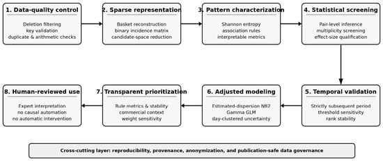
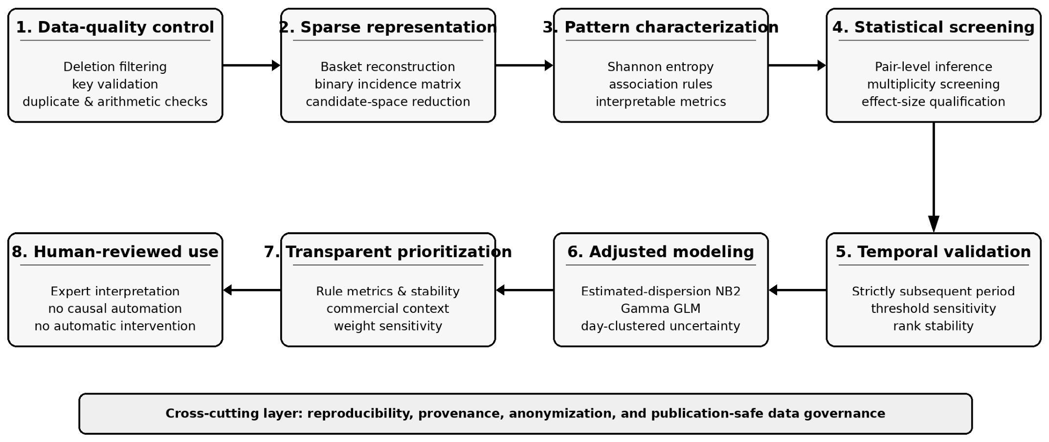
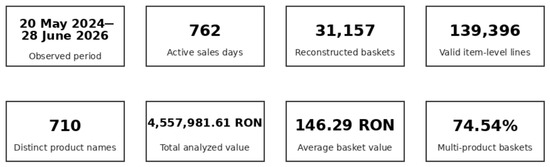
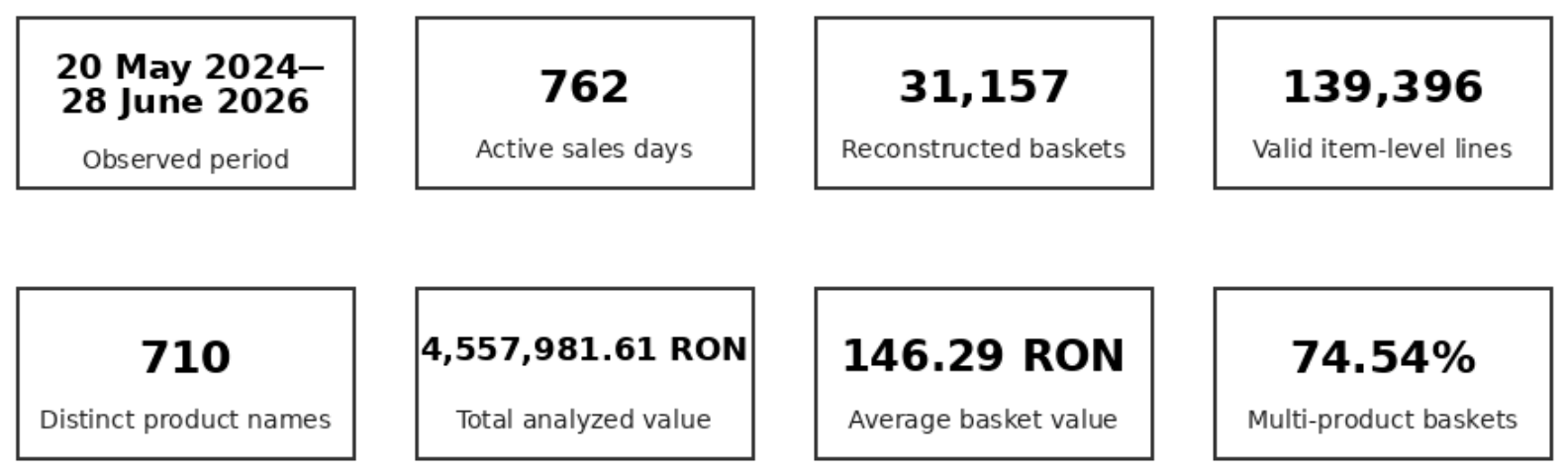
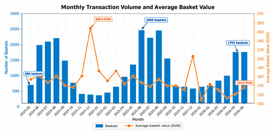
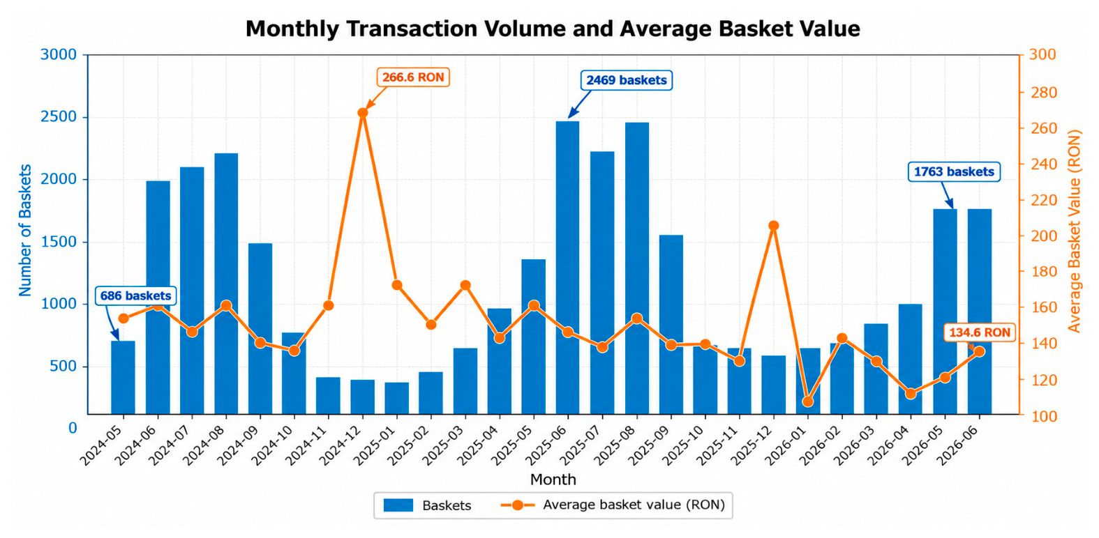
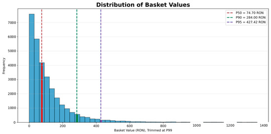
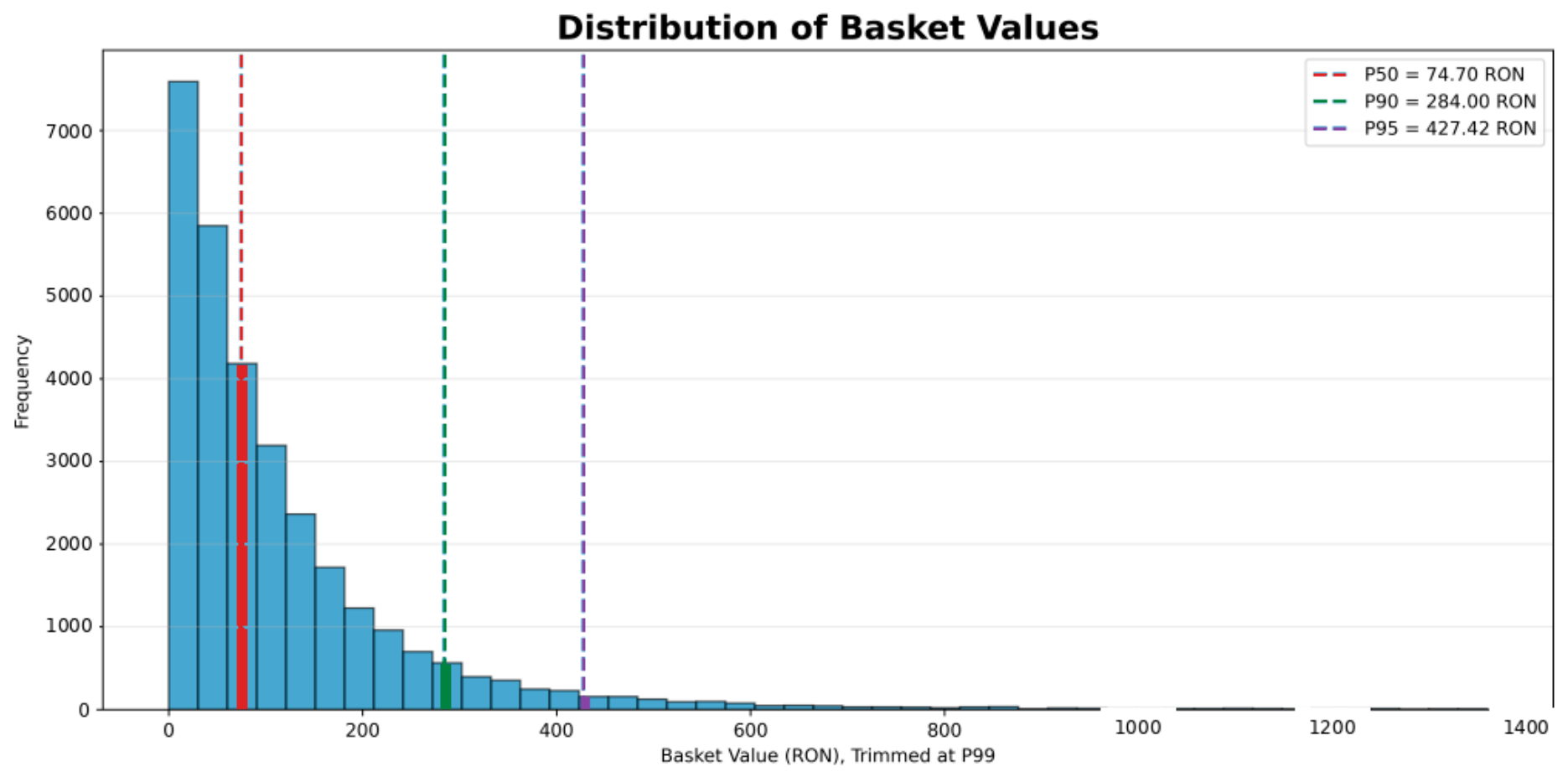
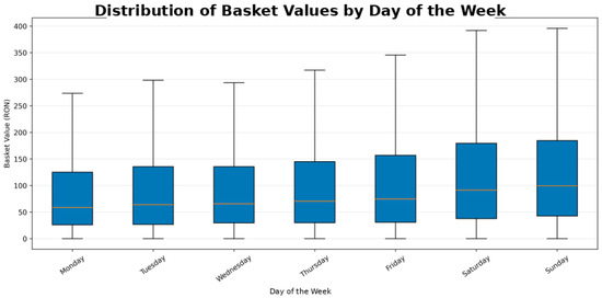
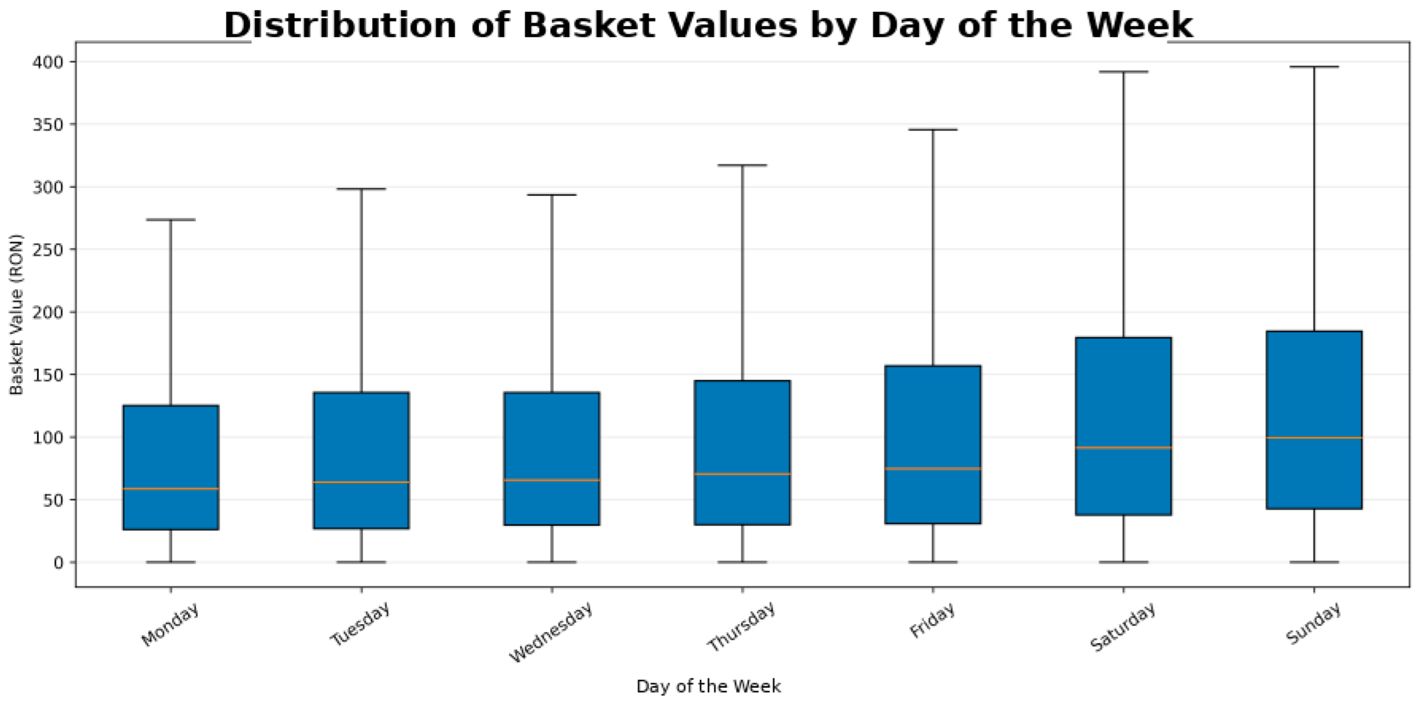
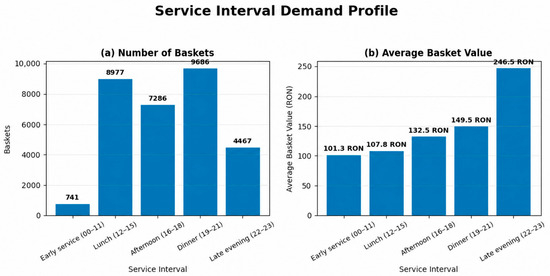
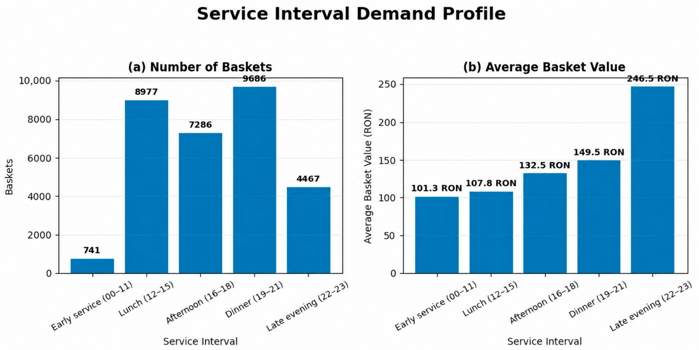
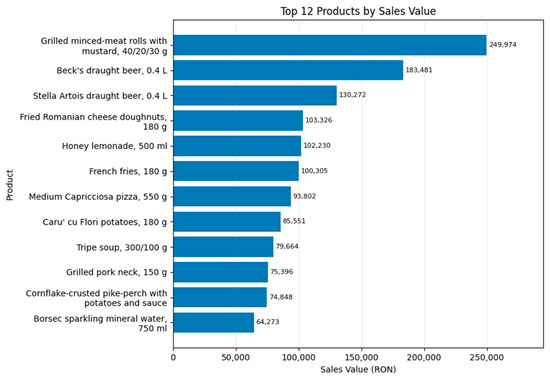
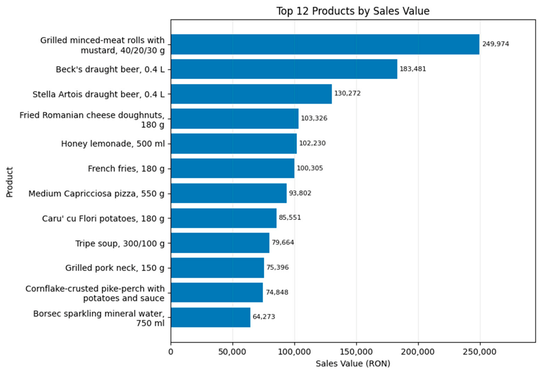
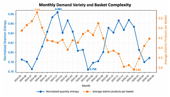
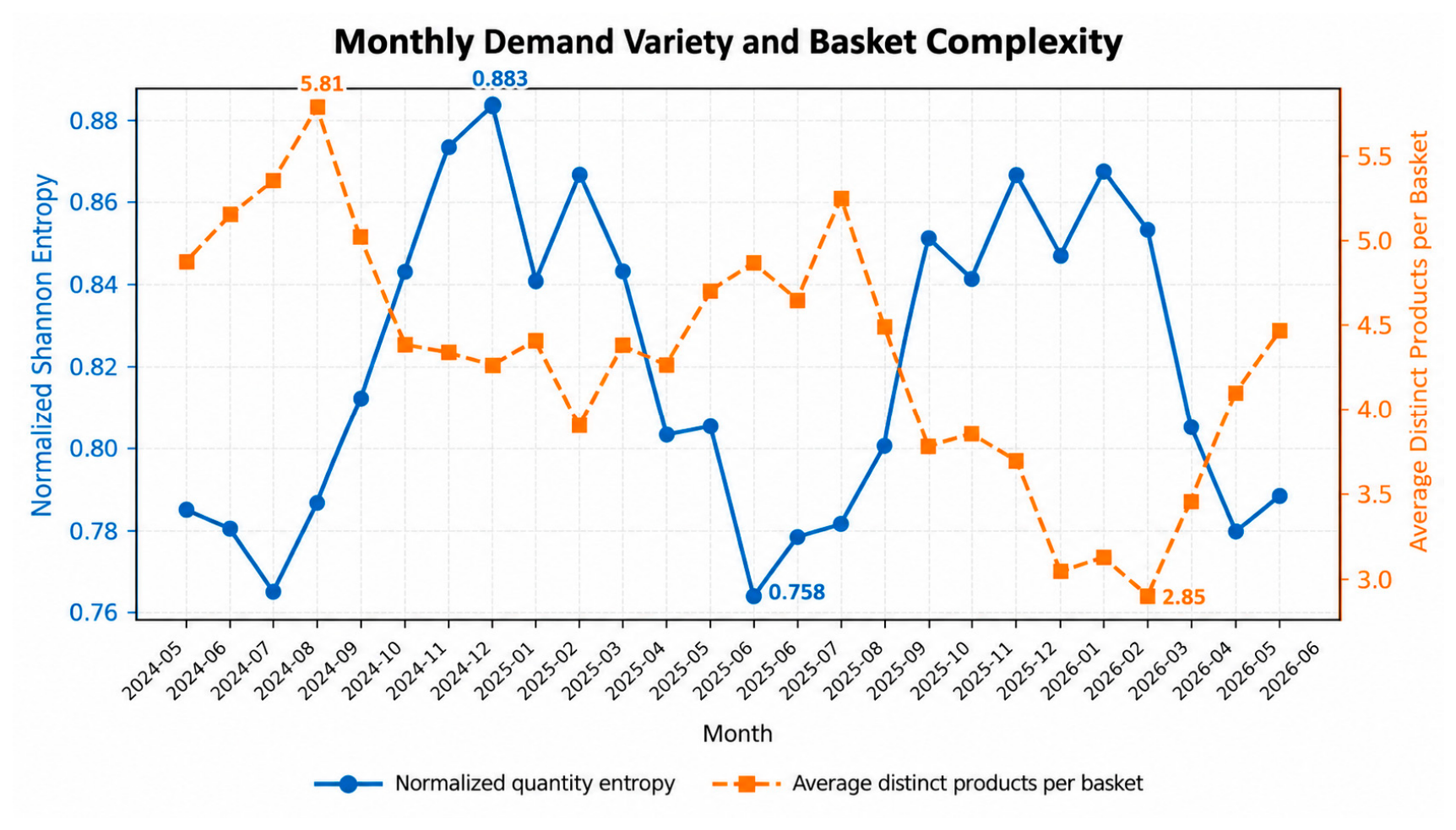
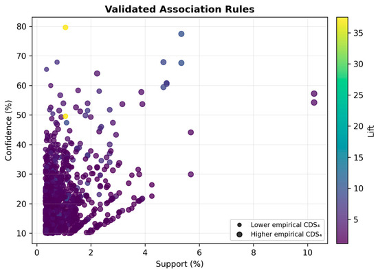
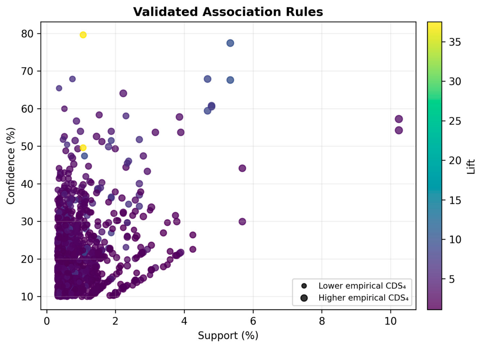
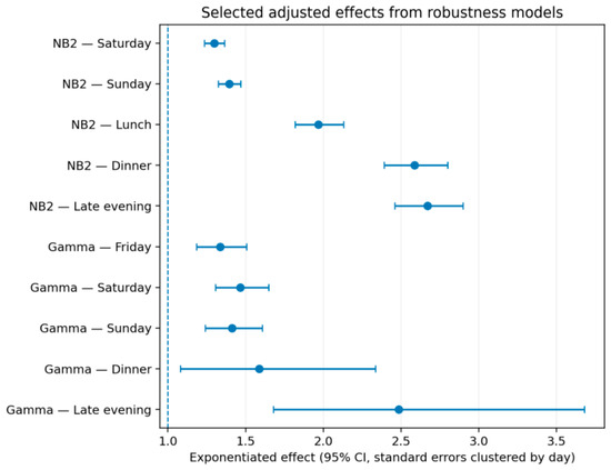
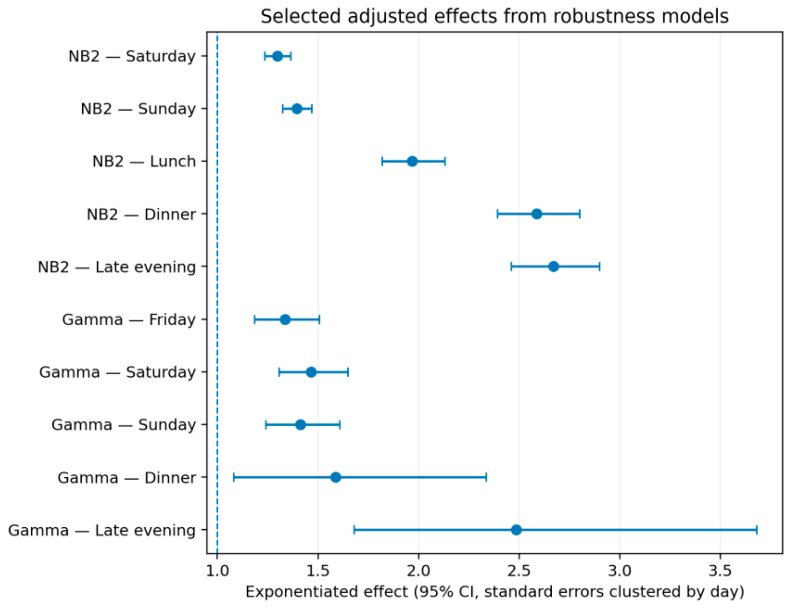
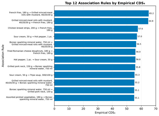
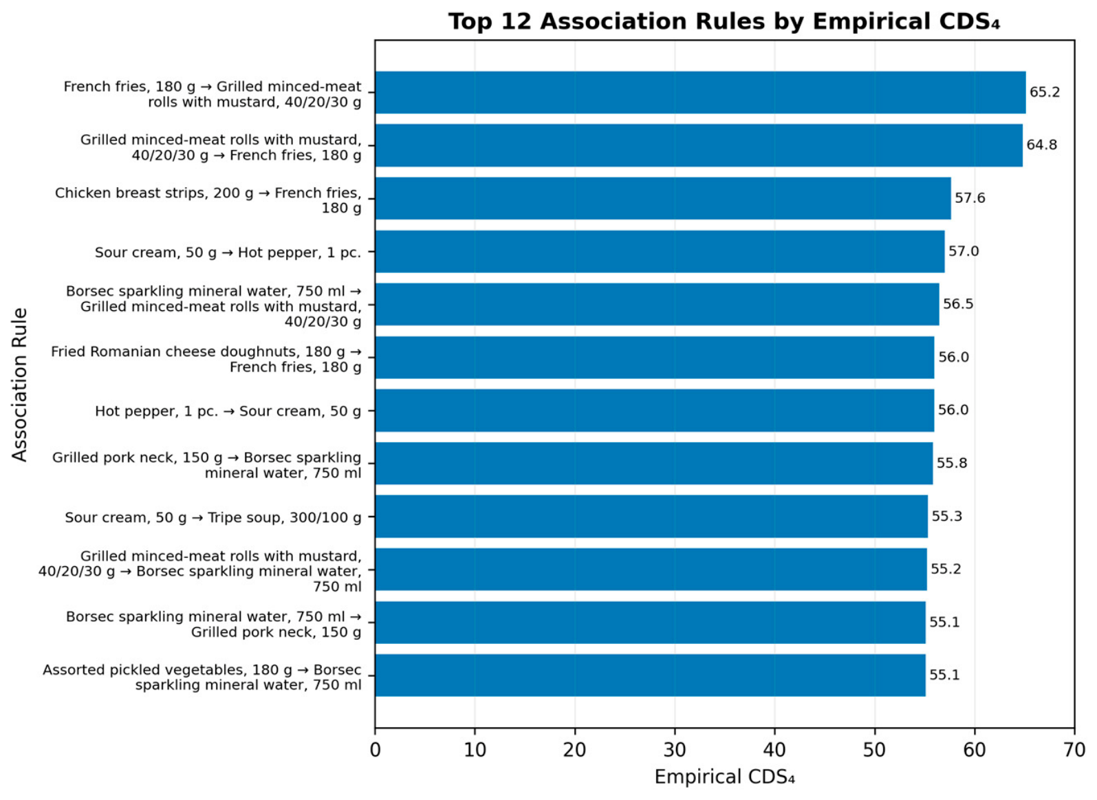
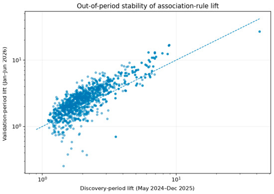
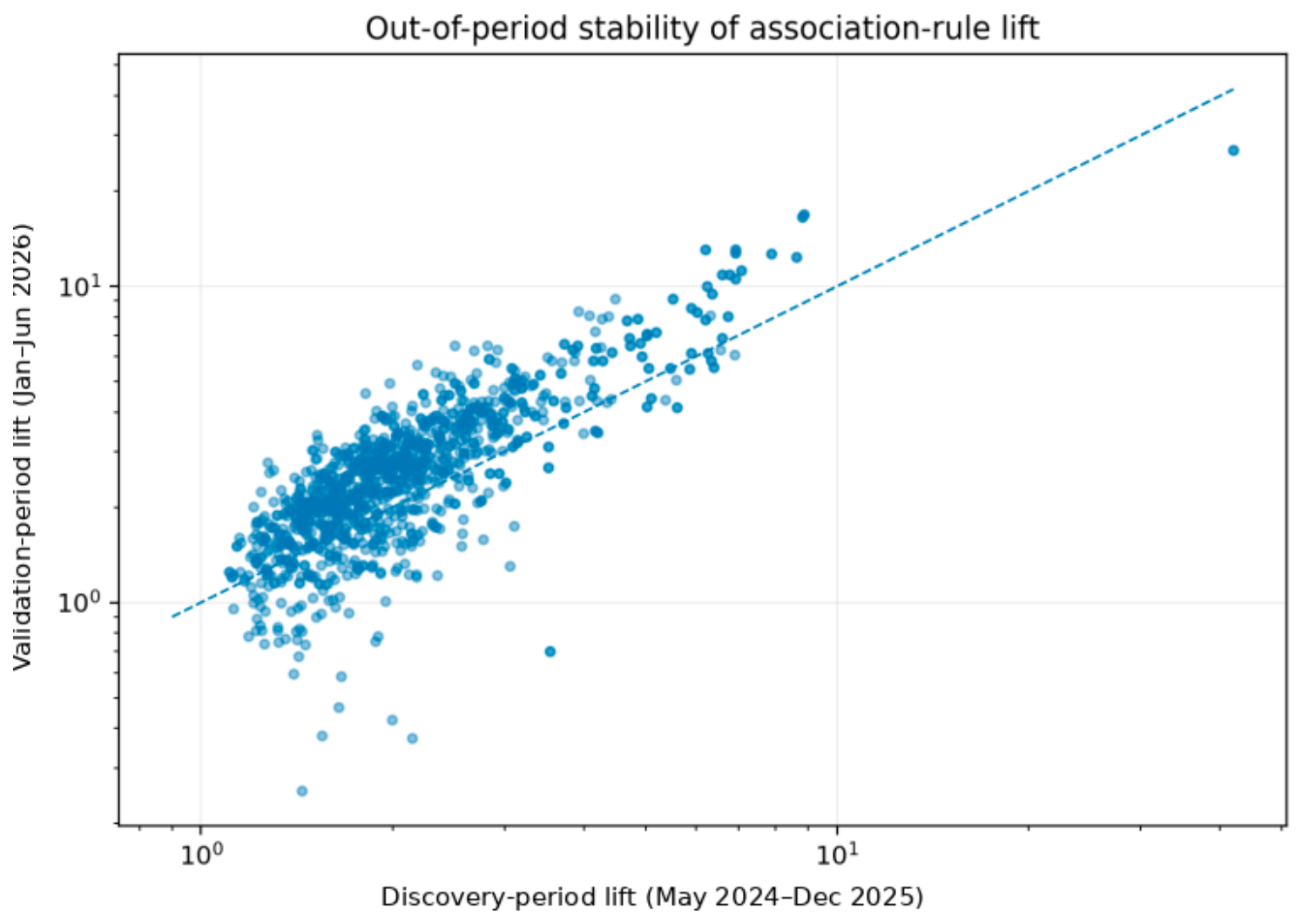
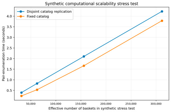
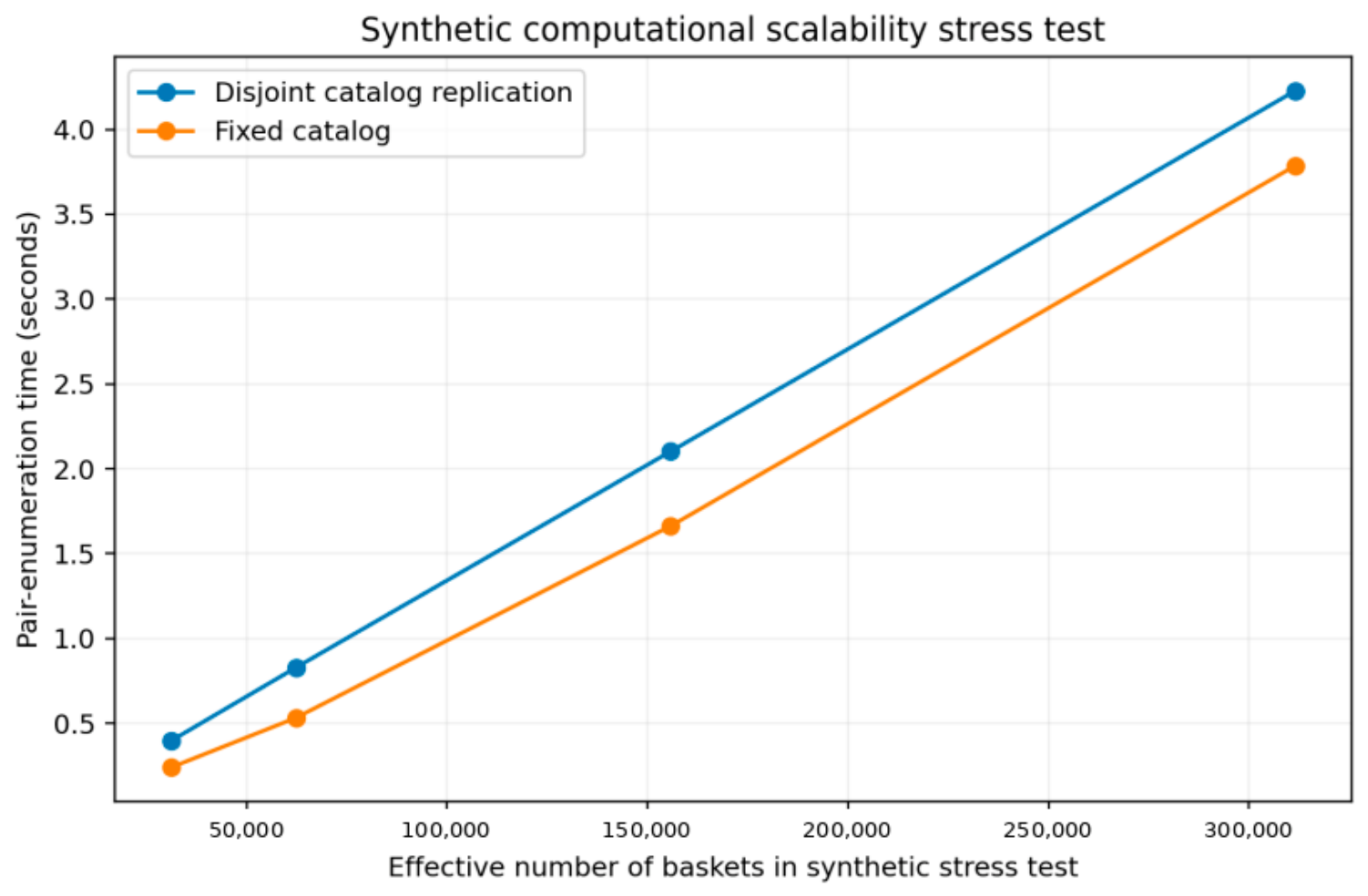

Disclaimer/Publisher’s Note: The statements, opinions and data contained in all publications are solely those of the individual author(s) and contributor(s) and not of MDPI and/or the editor(s). MDPI and/or the editor(s) disclaim responsibility for any injury to people or property resulting from any ideas, methods, instructions or products referred to in the content. |
© 2026 by the authors. Licensee MDPI, Basel, Switzerland. This article is an open access article distributed under the terms and conditions of the Creative Commons Attribution (CC BY) license.