


Abstract
Global optimization has become a cornerstone of modern machine learning, particularly for the challenging task of training high-dimensional neural network architectures. Despite the prevalence of established metaheuristics, traditional approaches frequently struggle with the irregular and multimodal error surfaces inherent in complex training landscapes. This paper proposes the parallel optimized particle swarm optimization (Parallel OPSO), a multi-population parallel framework specifically engineered to enhance the training efficiency and predictive accuracy of neural networks across classification and regression tasks. At its core, OPSO integrates several advanced mechanisms: a simulated annealing-based acceptance criterion to escape local minima, adaptive inertia weights that dynamically respond to stagnation by injecting momentum, and a hybrid Broyden–Fletcher–Goldfarb–Shanno (BFGS) local search phase for fine-grained convergence. While OPSO defines this underlying algorithmic model, Parallel OPSO represents its execution across parallel multi-population architectures. By partitioning the swarm into interacting subpopulations and leveraging modern multi-core architectures, Parallel OPSO significantly reduces training time, with prominent performance gains primarily manifesting on highly challenging and multimodal optimization tasks. Experimental evaluations demonstrate that while standard algorithms may perform adequately on simpler loss landscapes, Parallel OPSO achieves superior convergence robustness and accuracy when navigating demanding and highly irregular error surfaces. These results underscore Parallel OPSO as a highly efficient and scalable framework for optimizing neural network parameters in complex search spaces.
Keywords:
parallel metaheuristics; particle swarm optimization; neural network training; global optimization; hybrid local search; adaptive inertia; simulated annealing MSC:
65K05; 65K10; 68W01
1. Introduction
The training of artificial neural networks (ANNs) represents one of the most critical and challenging tasks in modern machine learning and computational intelligence [1,2]. From a mathematical perspective, training an ANN is formulated as a large-scale global optimization problem [3], where the objective is to minimize an error function by adjusting the network’s weights and biases. The global optimization problem is defined as
where the search space S is defined as the high-dimensional hyper-rectangle:
In the context of neural network training, the objective function represents the loss function (e.g., mean squared error or cross-entropy), and the vector contains the network’s parameters. This optimization landscape is highly non-linear, non-convex, and multi-modal, containing an immense number of local minima [4]. Apart from neural network training, this mathematical formulation finds critical applications in a variety of real-world problems, such as physics [5,6], chemistry [7], economics [8], and medicine [9,10]. Historically, optimization methods are divided into two main categories: deterministic and stochastic. Deterministic approaches, such as Interval methods [11,12] or gradient-based algorithms (e.g., backpropagation, stochastic gradient descent, Adam), rely on mathematical proofs or gradient derivatives to navigate the search space [13]. However, in high-dimensional and non-convex neural network landscapes, gradient-based methods are heavily prone to getting trapped in saddle points or sub-optimal local minima and are highly sensitive to initial weight configurations [4,13,14]. To overcome these limitations, stochastic and metaheuristic methods have been widely adopted. Guided by randomness, these methods do not guarantee finding the absolute global minimum in polynomial time, but they consistently locate high-quality solutions with remarkable implementation simplicity [15].
Researchers have proposed numerous stochastic algorithms, including controlled random search [16], simulated annealing [17,18], differential evolution [19], particle swarm optimization (PSO) [20,21], ant colony optimization [22], and genetic algorithms [23]. Furthermore, modern computational paradigms have successfully ported these algorithms to multi-core and GPU architectures to accelerate high-dimensional optimization [24,25], with comprehensive surveys available in recent literature [26,27].
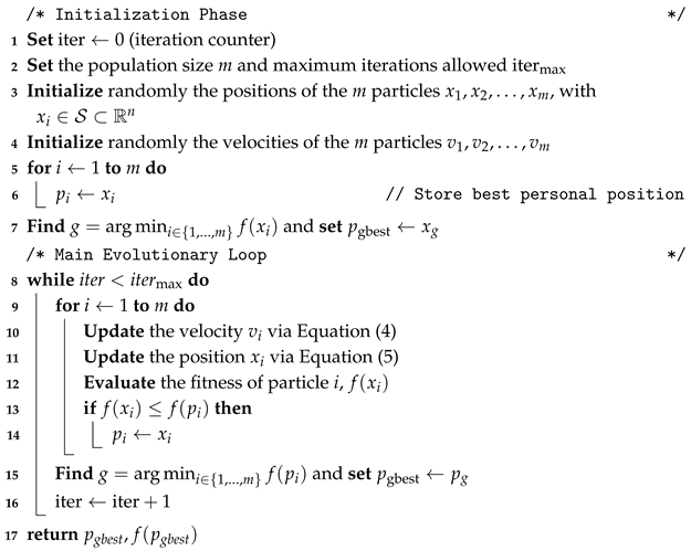
Among these metaheuristics, particle swarm optimization (PSO) has emerged as a highly efficient population-based algorithm inspired by the social behavior of bird flocking [28]. In PSO, a population of candidate solutions, called particles, explores the search space S. Each particle i is characterized by its current position and its velocity . The dynamic movement of each particle in a D-dimensional space is governed by updating its velocity and position at each iteration step [21,29] according to the following formulation:
where is the inertia weight introduced to control the impact of the previous velocity [30], and are the cognitive and social acceleration coefficients, and are uniformly distributed random numbers. The vector denotes the personal best position discovered by particle i, while represents the global best position found by the entire swarm. Despite its success, classical PSO can suffer from premature convergence and high computational costs when optimizing complex neural network architectures, falling into local minima during the exploitation phase [20,21]. Many researchers focus on dynamically adjusting the inertia weight [31,32] or integrating hybrid and parallel implementation techniques [33,34] to tackle complex numerical optimization problems. However, limited attention has been given to the simultaneous enhancement of scalability, multi-population parallel evolution, and adaptive convergence control in large-scale optimization environments. To address these challenges, this paper introduces the parallel optimized particle swarm optimization (Parallel OPSO) method, specifically engineered to enhance the training efficiency and predictive accuracy of neural networks. The proposed algorithm is a multi-population parallel framework that partitions the swarm into interacting subpopulations, leveraging modern multi-core architectures to significantly reduce execution time. More specifically, OPSO defines the core sequential optimization method that incorporates the enhanced search mechanisms, whereas Parallel OPSO extends this core engine into a cooperative, multi-threaded multi-population paradigm.
The novelty of Parallel OPSO lies in the integration of several advanced mechanisms within a unified parallel framework:
- Simulated Annealing Acceptance Criterion: A stochastic acceptance criterion is integrated to allow particles to occasionally accept worse positions, enabling the swarm to escape stubborn local minima [17,18].
- Adaptive Inertia Weight and Momentum: The inertia weight dynamically responds to swarm stagnation by injecting momentum, balancing wide-range exploration and local exploitation based on the algorithm’s real-time performance [32].
- Hybrid Local Search Phase: Incorporates a deterministic BFGS quasi-Newton method to refine promising candidate solutions and significantly enhance convergence accuracy toward the global optimum [35].
The main contributions of this work are summarized as follows:
- A parallel cooperative extension of the PSO algorithm, where the swarm is partitioned into multiple subpopulations evolving simultaneously on multi-core architectures using the OpenMP framework to enhance exploration in large-scale search spaces.
- A dynamic propagation mechanism that enables structured and controlled information exchange among the independent subpopulations, improving convergence speed while maintaining overall population diversity.
- The incorporation of adaptive inertia weight based on the framework introduced in [32], which dynamically responds to swarm stagnation by injecting momentum, effectively balancing global exploration and local exploitation based on the algorithm’s real-time performance.
- The integration of a simulated annealing-based stochastic acceptance criterion [17,18], which allows particles to occasionally accept worse positions, providing a robust mechanism to escape stubborn local minima.
- The incorporation of a hybrid local search phase utilizing the deterministic BFGS quasi-Newton method [35] to significantly improve convergence accuracy and speed up the localization of the exact global optimum.
- A comprehensive experimental evaluation spanning both large-scale global optimization benchmark problems and demanding neural network training tasks for classification and regression, demonstrating that Parallel OPSO consistently converges to more robust solutions compared to state-of-the-art algorithms.
The remainder of this article is organized as follows: Section 2 outlines the foundational background of classical PSO alongside the detailed mathematical formulation of the proposed Parallel OPSO; Section 4 presents the experimental setup, benchmark functions, and comparative performance analysis; and finally, Section 5 summarizes our key findings, provides concluding remarks, and outlines directions for future research.
2. Background Materials
This section begins with the main aspects of the original PSO method and continues by presenting in detail the main parts of the proposed method.
2.1. Artificial Neural Networks and Training Process
Artificial neural networks (ANNs) are computational models inspired by biological nervous systems, structured to approximate complex non-linear functions and identify high-dimensional data patterns [1,13]. An ANN typically comprises interconnected processing units (neurons) organized into sequential layers: an input layer that accepts raw feature vectors, one or more hidden layers that extract hierarchical representations, and an output layer that delivers final estimations or classifications [13]. Each inter-neuron connection is weighted by an adjustable parameter, and individual nodes apply non-linear activation functions to modulate incoming signals [13].
The training process of an artificial neural network involves iteratively modifying its internal weights and biases to minimize the discrepancy between predicted outputs and known ground-truth targets [1,13]. This optimization mechanism operates through two primary computational stages:
- Forward Propagation: Input data propagate sequentially through the network layers, where weighted sums are computed and passed through non-linear activation functions to generate a prediction [1,13].
- Backward Propagation (Backpropagation): The output error is quantified using a predefined loss function, and error gradients with respect to network parameters are calculated utilizing the chain rule [13,14].
Conventionally, gradient-based optimization techniques update connection weights iteratively along the error landscape [14,35]. Because neural network training landscapes are typically high-dimensional, non-convex, and prone to severe stagnation in local attractors [4], advanced global optimization and meta-heuristic frameworks are frequently applied to optimize or assist in training neural network architectures [2,15,26].
2.2. Classical Particle Swarm Optimization (PSO)
The classical particle swarm optimization (PSO) algorithm, originally introduced by Kennedy and Eberhart [29], is a population-based stochastic optimization technique inspired by the social behavior of bird flocking or fish schooling. The algorithm explores an n-dimensional continuous search space using a population of m interacting agents called particles. Each particle i ( is characterized by its dynamic state parameters, consisting of an n-dimensional position vector and a corresponding velocity vector During the optimization process, each particle maintains a memory of its own historical personal best position discovered so far, denoted as . Concurrently, the swarm tracks the absolute global best position achieved by any particle in the entire population, defined as , where represents the objective function under minimization. To balance global exploration and localized exploitation, a trade-off extensively evaluated in recent metaheuristic literature [2,3], Shi and Eberhart [30] introduced the inertia weight factor . At each discrete evolutionary epoch t, the dynamic trajectories of the particles are updated according to the following stochastic kinematic equations:
where is the inertia weight, and denote the cognitive and social acceleration coefficients, respectively, and represent independent uniformly distributed random vectors injected to maintain stochastic diversity. Despite its mathematical simplicity and high convergence speed, the classical formulation is prone to stagnation in complex multimodal landscapes due to rapid loss of population diversity, a challenge frequently highlighted in modern optimization benchmarks [20,36]. The main parts of the original PSO method are listed in Algorithm 1.
| Algorithm 1: The classical PSO algorithm. |
 |
3. The Proposed Method
3.1. Parallel Optimized Particle Swarm Optimization Algorithm
The distributed framework of the optimized particle swarm optimization (OPSO) algorithm is engineered by partitioning the global agent population into K distinct subpopulations, and it is presented graphically in Figure 1. Each subpopulation operates as an autonomous evolutionary unit allocated to an individual processing element, enabling simultaneous execution across a shared-memory environment [37].
Figure 1.
Schematic representation of the Parallel OPSO framework architecture. The central OpenMP shared-memory region manages thread spawn and execution across K autonomous subpopulation islands (Island 1 through Island K). Red directional arrows illustrate the dynamic inter-island migration topologies, depicting both single-target routing (1-to-1, 1-to-N) and multi-island coordination mechanisms (N-to-1, N-to-N) used for periodic elite candidate solution exchange.
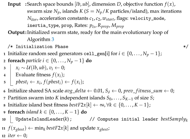
Before initiating the optimization cycle, the multi-swarm configurations are established, and the global termination strategy () is selected during the initialization phase (Algorithm 2). To govern decentralized convergence behavior and manage interaction dynamics between the concurrently evolving swarms, the architecture introduces a set of control features: a topological propagation method (), a generational communication rate (), a volumetric quantity of migrated solutions (), and a localized termination criterion () [34,38].
| Algorithm 2: Optimized and parallel particle swarm optimization (OPSO)—initialization phase. |
 |
The communication frequency across the multi-swarm layout is controlled by the propagation rate , which establishes the exact number of generational steps between consecutive data distributions. Low values for enforce tight coupling and frequent interaction, a configuration that can accelerate convergence velocities but risks collapsing population diversity [38,39]. Conversely, high values for grant the individual islands extended periods of decoupled execution, fostering independent exploration of unmapped solution regions.
In a similar manner, the volume of shared elite information is dictated by the parameter , which defines the number of top-performing vectors transmitted during a migration step. Expanding strengthens the collective exploitation capability by injecting high-quality geometric coordinates into target swarms; however, excessive data injection can induce premature convergence by steering all independent groups toward identical local optima [38,39,40]. Within this framework, the specific bounds for and are derived through systematic empirical tuning to maintain a healthy balance between localized search refinement and global space exploration, with the precise values detailed in the Experimental Results section.
During every generational step, the system monitors each subpopulation to determine if it has met its localized termination criterion , which is evaluated independently via an advanced convergence heuristic known as the similarity check [41]. The total number of stagnated units is then cross-referenced with a macro-level decision threshold, denoted as Q. This threshold mathematically operationalizes the chosen system-wide termination strategy to govern the macro-level optimization loop [38,41]:
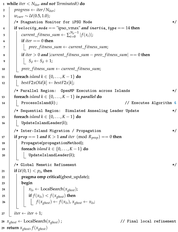
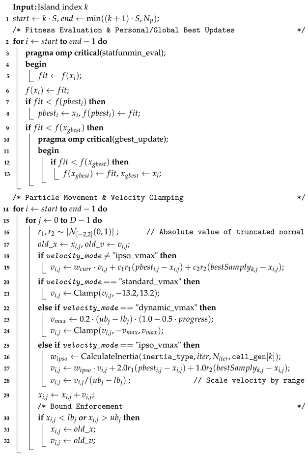
Following the calculation of the threshold metrics, the subpopulations proceed with their parallel evolutionary operations, executing localized kinematics updates and simulated annealing leader adjustments as detailed in Algorithm 4. At generational intervals matching the propagation rate , the main execution loop (Algorithm 3) triggers the designated migration topology to distribute elite candidate vectors across the multi-threaded network [34,38,40].
| Algorithm 3: Optimized and parallel particle swarm optimization (OPSO)—main evolutionary loop (continues from Algorithm 2). |
 |
| Algorithm 4: ProcessIsland(k): parallel fitness evaluation and particle update for island k (invoked from the parallel region of Algorithm 3). |
 |
The iteration counter increments, and the status of the threshold criterion Q is evaluated. If the conditions for global termination are not fulfilled, the concurrent optimization sequence continues. Upon satisfying the macro-level stopping condition, the framework (Algorithm 3) invokes a memetic refinement sequence, executing a rigorous local search directly around the global best solution to secure high-precision mathematical accuracy before returning the final optimized result [42].
From an architectural standpoint, mapping each subpopulation to an isolated thread or processing core facilitates true concurrent execution. Synchronization barriers are strictly confined to the scheduled propagation phases, allowing the swarms to evolve independently during intermediate generations and significantly minimizing memory access latencies [34]. Resource utilization is optimized through the selection of the global termination strategies (ANY, MAJORITY, ALL), which prevent thread starvation and idle processing states by eliminating the requirement for all processing elements to terminate at the same time. The ANY strategy, in particular, permits rapid continuation by halting the global loop the moment early convergence is detected on any single thread via the similarity metric [41]. While selecting the ANY global termination strategy () prioritizes computational efficiency and drastically reduces execution time by eliminating idle processor states, it inherently carries a potential risk of premature termination if a single isolated subpopulation converges early to a local attractor. Within our framework, this risk is directly mitigated by two structural safeguards: (i) the mandatory warm-up phase (), which suppresses localized termination diagnostics during early stochastic iterations, and (ii) the continuous inter-island migration mechanism (), which routinely injects high-quality solution coordinates across all subpopulations to maintain global diversity and prevent single-island stagnation. Furthermore, the computational footprint of the migration phase remains small, as it restricts communication to a limited set of elite solution coordinates. This brief coordination phase introduces negligible latency relative to the overall objective function evaluation costs, and it significantly enhances optimization performance by enabling effective information sharing across the parallel architecture [34,38].
3.2. Inter-Swarm Communication Protocol and Migration Topologies
Within the cooperative execution phase of the parallel framework, the communication layer facilitates the distribution of high-quality parameter configurations among the concurrent islands. When the scheduled migration interval conditions are satisfied, the elite solution vectors identified by a specific subpopulation are transmitted across the shared-memory space to overwrite the lowest-performing coordinates of the designated target swarms. The foundational objective of this information routing scheme is to optimize cross-island exploration, ensuring that promising topological discoveries are rapidly assimilated into the broader optimization landscape within the main evolutionary loop (Algorithm 3) to enhance overall convergence efficiency [34,38].
Unlike conventional distributed metaheuristics that rely on static and rigid structural layouts, such as ring, star, or fully mesh migration topologies, the proposed framework introduces a localized, dynamically configurable migration model tailored for high-dimensional execution spaces. Conventional geometric topologies impose strict synchronization locks and significant thread contention penalties as the execution scale grows, which frequently induces severe memory access latencies within shared-memory architectures [34,38]. To avoid structural complexity and eliminate excessive communication overhead, the parallel architecture relies on a versatile routing protocol operating across four discrete configuration states:
- One-to-One (): A single source subpopulation, selected uniformly at random, migrates its historical elite parameter states exclusively to a single target subpopulation, which is also designated through a random uniform distribution.
- One-to-All (): A randomly isolated subpopulation serves as a central broadcaster, transmitting its optimal geometric updates to refresh the search vectors of all other active swarms simultaneously.
- All-to-One (): Every active computational swarm routes its current top-performing vectors toward a single, randomly targeted subpopulation, consolidating global directional data into a localized spatial window to catalyze structural exploitation.
- All-to-All (): A dense execution mode where every individual subpopulation synchronizes and exchanges its finest candidate solutions with the historical memory matrix of every other swarm in the network.
By adjusting the combination of these topological routing strategies alongside the volumetric payload parameter , the OPSO framework maintains a fluid balance between regional exploitation and global population diversity [34,38]. This dynamic coordination mitigates structural stagnation risks while preserving the low coordination footprint required for efficient execution on multi-core compute clusters.
3.3. Adaptive Inertia Weight Mechanism
To achieve a self-regulating balance between global exploration and localized exploitation, each autonomous subpopulation discards static or strictly time-dependent parameter scaling. Instead, an adaptive inertia weight mechanism is implemented [31] within the per-island parallel update procedure (Algorithm 4), adapting the phenotypic stagnation-tracking framework introduced in the ideal particle swarm optimization (IPSO) architecture [32]. This framework evaluates the state of the swarm by monitoring the phenotypic convergence rate across consecutive generations. When the global fitness gradient flattens, indicating that the multi-swarm trajectory is confined within a local attractor, the inertia weight parameter is dynamically adjusted to modulate particle momentum.
Operationally, the system calculates the absolute differential progress of the collective fitness landscape at every iteration. If the fitness deviation between sequential states falls below a predefined threshold, a stagnation counter increments. By calculating the ratio of cumulative stagnant states against the elapsed generational counter, a dynamic constraint coefficient is derived. Consequently, when the subpopulation actively discovers novel structural minima, the velocity profile maintains a high exploratory momentum. Conversely, when severe multi-island stagnation is detected, the inertia scales down to its minimum operating boundary, dampening particle velocities to focus computational resources strictly on high-precision local exploitation [31,32].
Mathematical Formulation
The evolutionary state monitoring is governed by evaluating the global fitness volume change at each generation t, tracking structural stagnation vectors as formalized in the IPSO framework [32]:
where m denotes the number of particles within the subpopulation, and represents the objective cost value of the i-th particle at generation t. The localized stagnation state indicator is defined as
Using the real-time feedback from , the cumulative stagnation tracking matrix and its corresponding density ratio are computed dynamically:
The adaptive inertia weight supplied to the velocity kinematic updating core (Algorithm 4) is formally governed by the bound-constrained formulation [32], building upon the dynamic inertia weight control concepts introduced in [30]:
where and represent the predefined boundary coefficients governing the dynamic momentum spectrum.
3.4. Adaptive Simulated Annealing Acceptance Criterion
To balance the exploitation of local optima with the necessity of maintaining exploratory pressure, a stochastic acceptance mechanism is integrated into the leader update phase of each island. Traditional PSO variants typically employ a greedy selection rule, which often leads to rapid convergence toward suboptimal regions in non-convex, high-dimensional landscapes [21,28]. To mitigate this, our approach implements an adaptive simulated annealing acceptance criterion during the subpopulation update (Algorithm 4), allowing the sub-population leader () to occasionally accept inferior solutions based on a temperature-dependent probability inspired by the classic simulated annealing framework [5,17,18].
Let represent the fitness difference between the current best particle within sub-cluster and the recorded sub-cluster leader. The probability of accepting a potentially worse configuration is defined as
where T represents the current normalized temperature under a linear cooling schedule, calculated as to enforce a minimum thermal floor, withprogressdenoting the relative execution progress (). To ensure robustness across diverse objective function scales, an adaptive scaling factor is maintained locally for each sub-cluster k, updating incrementally via an exponential moving average (EMA) as for every positive fitness delta observed. The term serves as a numerical stability constant to prevent division by zero.
The parameters governing the thermal schedule were selected based on preliminary sensitivity tests balancing exploration and computational stability. A dynamic linear cooling schedule provides a smooth transition from stochastic global sampling in early stages to deterministic local convergence near termination. The thermal floor () avoids numerical underflow, while the EMA smoothing coefficient of ensures that scale updates reflect long-term landscape trends without overreacting to transient gradient spikes.
This mechanism facilitates a transition from a high-exploration phase at the onset of the optimization process, where the acceptance of inferior moves enables the algorithm to escape local attractors, to a high-exploitation phase as T approaches zero, effectively narrowing the search towards the global optimum [17,18]. By decoupling the leader update from strict greedy selection, the algorithm exhibits enhanced resilience against the “saddle point” problem in high-dimensional spaces [4], ensuring a more thorough traversal of the search space before settling into a terminal configuration [11,12]. This adaptive control, combined with the parallel island model paradigm, provides a robust defense against premature stagnation without the prohibitive computational overhead associated with global, non-localized simulated annealing schedules [32,34,39,40].
3.5. Hybrid Local Search Phase
To balance global stochastic exploration with high-precision exploitation, Parallel OPSO incorporates a memetic hybrid local search phase [42] based on the deterministic Broyden–Fletcher–Goldfarb–Shanno (BFGS) quasi-Newton algorithm [35]. During execution, the local search procedure is stochastically triggered on the global best position within the main evolutionary loop (Algorithm 3) with a predefined probability In our experimental configuration, was set to during the main execution iterations. This choice is intentional: extensive preliminary tuning revealed that applying full gradient-based BFGS evaluations at every generation incurs prohibitive computational overhead due to numerical finite-difference gradient estimations. By restricting BFGS refinement exclusively as a final deterministic post-processing step on , Parallel OPSO preserves high overall computational throughput while ensuring high-precision terminal convergence.
To prevent race conditions during parallel island evaluations, this stochastic triggering and the subsequent update are synchronized across threads using OpenMP critical sections (#pragma omp critical). Additionally, a final deterministic refinement step is mandatorily executed inside the routine upon meeting the swarm stopping criteria, applied strictly to the global best position , once the swarm reaches full convergence, defined by a similarity check criterion requiring 25 consecutive unchanged iterations per island. When invoked, each local search phase is allocated a maximum budget of 2000 iterations (function evaluations). The BFGS procedure [35] terminates when any of the following stopping criteria are satisfied: (i) no further reduction in the objective function value can be achieved during line search, or (ii) the maximum iteration limit of 2000 evaluations is reached.
The BFGS algorithm iteratively refines the target position vector along a search direction , where the gradient vector is numerically approximated via finite differences and represents an approximate inverse Hessian matrix. At each local step k, is dynamically updated using the spatial difference vector and the gradient difference vector according to
where . The refined candidate position replaces strictly under a greedy scheme, updating the global optimum only if . This gradient-based coupling guarantees superlinear local convergence characteristics, refining the stochastic candidate solutions of OPSO to exact numerical optima.
3.6. Subpopulation Termination Criterion via Similarity Check
In parallel multi-swarm architectures, determining the optimal execution boundary for each autonomous subpopulation is critical. Halting an island prematurely deprives the global swarm of valuable population diversity and high-quality coordinates during migration phases [39,40]. Conversely, allowing a stagnated subpopulation to execute until the global maximum iteration limit leads to wasted processor cycles and unnecessary energy consumption [34,38]. To resolve this trade-off, each individual island k dynamically monitors its own search trajectory during its iteration updates (Algorithm 4) via a localized termination state .
To ensure sufficient initial exploration and avoid false positive termination signals caused by early stochastic fluctuations, a mandatory warm-up period is enforced. Localized convergence diagnostics remain inactive until the generation counter satisfies:
Upon crossing this threshold, the algorithm tracks the fitness progression of island k at every generation t by calculating the absolute difference between its current and previous local best objective values:
To evaluate whether reflects genuine mathematical convergence rather than a transient plateau, the framework embeds the similarity check heuristic proposed by Tsoulos et al. [41]. Conventional termination metrics often rely on instantaneous point-to-point differences, making them highly sensitive to noise in complex fitness landscapes. Specifically, island k is declared locally converged () when the average objective improvement falls below a predefined tolerance threshold :
In contrast, the similarity check evaluates the convergence behavior over a sliding historical window of W = 25 consecutive iterations. This window size was determined through empirical sensitivity trials evaluating window sizes in the range W in [10, 40] across five representative datasets (Wine, Pima, WDBC, Spiral, and Ecoli). As summarized in the Table 1, a setting of W = 25 offered the optimal baseline balancing convergence reliability and computational speed. Smaller window sizes (W < 20) risk premature island termination due to transient objective plateaus—as evidenced by elevated error rates on datasets such as Wine (19.12%). Conversely, excessively large windows () yield no tangible accuracy gains and, in cases like Wine and WDBC, significantly degrade classification precision while systematically escalating computational overhead up to 1.06 s per fold. Consequently, W = 25 represents a robust trade-off, ensuring stability against false positive termination without incurring unnecessary computational latency.
Table 1.
Sensitivity analysis of similarity check window parameter (W).
From an implementation perspective, each parallel worker thread maintains an isolated heuristic evaluator instance (threadSimilarity[k]). This design eliminates thread contention and lock overheads, enabling fully decoupled convergence checks across processing cores [34,37]. The aggregate count of stagnated islands is continuously tracked as
where denotes the indicator function. When the global termination strategy evaluated in the main loop (Algorithm 3) is triggered [38,41]. Finally, the maximum iteration count serves as an absolute safety ceiling (), guaranteeing bounded computational time under all execution conditions.
3.7. Pseudocode and Algorithmic Summary
The complete metaheuristic workflow of the proposed parallel optimized particle swarm optimization algorithm, incorporating the parallel migration topologies, adaptive inertia weight control mechanisms, simulated annealing leader acceptance criteria, and hybrid local search refinement, is synthesized in the following pseudocode, presented across three parts to preserve legibility: the initialization phase (Algorithm 2), the main evolutionary loop (Algorithm 3), and the per-island parallel update procedure invoked within it (Algorithm 4):
Algorithm 2 performs the sequential initialization of the swarm, the islands, and the initial leaders. The resulting state is then evolved by the main loop of Algorithm 3, which repeatedly invokes, within its OpenMP parallel region, the per-island update procedure detailed separately in Algorithm 4.
Additionally, Algorithm 3 relies on two key sub-routines: updates the leader of each island using a Simulated Annealing-based acceptance criterion to escape local minima, while manages inter-island communication by migrating candidate solutions across subpopulations according to the specified topology.
Algorithm 4 specifies the computations carried out independently and concurrently for each island during every generation of the main loop, namely the fitness evaluation and personal/global best updates, followed by the particle movement, velocity clamping, and bound enforcement steps.
3.8. Computational Complexity Analysis
The computational complexity of the proposed algorithm is analyzed per iteration, considering the number of particles N, the dimensionality of the search space D, and the number of subpopulations (islands) K. Let be the number of particles per island. The total complexity per iteration is dominated by the evaluation of the objective function, the velocity/position updates, the hybrid local search procedure, and the communication overhead. The breakdown is as follows:
- Objective Function Evaluation: The primary cost is associated with the evaluation of the objective function. In each iteration, N evaluations are performed. If denotes the computational cost of the objective function , the complexity is . Due to the OpenMP parallelization, this is distributed across K threads, reducing the execution time to per thread, assuming uniform load balancing [34,37].
- Particle Update Mechanism: The velocity and position update operations for all N particles across D dimensions, executed concurrently within the subpopulation update procedure (Algorithm 4), require time. Similar to the objective function, this is parallelized as per subpopulation [30,34].
- Hybrid Local Search Phase: The deterministic BFGS quasi-Newton refinement is stochastically invoked on the global best solution within the main evolutionary loop (Algorithm 3) with probability . Let denote the average number of objective function evaluations required by the BFGS gradient calculations and line search per local execution. The computational cost of matrix updates for a D-dimensional search space is . Thus, the amortized cost per iteration for the hybrid refinement phase is [35,42].
- Inter-Island Propagation: The migration mechanism triggered within the main execution loop (Algorithm 3) involves sorting particles by fitness within subpopulations and transferring them. Sorting n particles takes . Given that the migration occurs every P iterations (propagation rate), the amortized complexity per iteration for the migration phase is [34,39,40].Combining the above, the total computational complexity per iteration is expressed asAs P is typically significantly larger than 1 (e.g., ) and the local search activation probability is set to zero (), any potential local search computational overhead is completely eliminated, leaving only negligible propagation overhead relative to objective function evaluations. Consequently, the algorithm exhibits linear scaling with respect to the number of particles and dimensions, while parallel efficiency is optimized by the factor K, allowing the algorithm to maintain high performance in high-dimensional optimization problems [27,34,38].
4. Results
4.1. Experimental Datasets
The datasets used in the conducted experiments were downloaded from the following online databases:
- The UCI website. https://archive.ics.uci.edu/ (accessed on 24 June 2026) [43]
- The Keel website. https://sci2s.ugr.es/keel/datasets.php (accessed on 24 June 2026) [44].
The datasets used in the conducted experiments are shown in Table 2.
Table 2.
Summary and main characteristics of the experimental datasets.
4.2. Experimental Settings
The software used in this work was entirely coded in ANSI C++ with the support of the OPTIMUS environment, downloaded from https://github.com/itsoulos/OPTIMUS/(accessed on 24 June 2026) [77]. All the experiments were conducted on an AMD Ryzen 5950X with 128GB of RAM and the operating system used was Debian Linux. During the experimental evaluation, a 10-fold cross-validation procedure was applied, in which each dataset was divided into ten subsets (folds). In each validation round, 90% of the instances were used for training, whereas the remaining 10% were reserved for testing. To ensure statistical reliability, each experimental configuration was independently executed 30 times, with a different initialization seed assigned to the random number generator for each run. The random numbers required during the experiments were generated using the ‘drand48()‘ function provided by the C standard library. The average classification error is defined as
where the set T represents the associated test set, with . The settings used in the conducted experiments are shown in Table 3.
Table 3.
Values for the experimental parameters.
Moreover, the following notation is used in the tables presenting the experimental results:
- The column DATASET indicates the name of the used dataset.
- The column BFGS is used for the application of the BFGS optimization procedure [78] to train an artificial neural network [79,80] with 10 processing nodes.
- The column NEAT [81] represents the results obtained by the NEAT (NeuroEvolution of Augmenting Topologies) method.
- The column RBF denotes the usage of a radial basis function (RBF) network [82,83] with 10 processing nodes.
- The column GEN denotes the incorporation of a genetic algorithm [84] with the same parameters as in the proposed method. This algorithm was used to train an artificial neural network with 10 processing nodes.
- The column OPSO stands for the results obtained by the incorporation of the proposed method.
- The row labeled AVERAGE presents the mean classification error obtained across the entire collection of datasets.
4.3. Parallel Performance and Scalability Analysis
To thoroughly evaluate the computational advantage of the proposed parallelized scheme, benchmarking experiments were conducted across all 20 datasets using 1, 2, 5, and 10 threads. Table 4 summarizes the execution metrics, including wall-clock runtime (), speed-up ratio (), parallel efficiency (), and CPU utilization (%).
Table 4.
Parallel performance metrics including Wall-Clock Time ( in seconds), Speed-up (), Parallel Efficiency (), and CPU Utilization across different thread configurations ().
As observed in Table 4, expanding the thread pool leads to a consistent reduction in total execution time across all datasets. For instance, on the Spiral dataset, wall-clock time drops from 3.54 s (1 thread) to 0.70 s (10 threads), achieving a speed-up factor of 5.06 times. Notably, several datasets (e.g., Pima, Spiral, and Saheart) exhibit super-linear speed-up under 2 threads (), which is attributed to localized cache efficiency advantages and stochastic early convergence in the island subpopulations.
As thread counts scale up to 10, CPU utilization closely matches full capacity (~980–990%), demonstrating effective thread utilization. However, parallel efficiency shows an expected decrease, settling between 25% and 50% across most datasets. This behavior is primarily driven by inter-island communication overhead. During periodic migration phases, thread synchronization barriers and data exchange mechanisms (e.g., solution transfer and memory locks) introduce latency that scales with the number of concurrent subpopulations. Nevertheless, the substantial reduction in total runtime confirms that the parallel implementation delivers substantial performance gains, ensuring fast execution for complex optimization runs.
4.4. Comparison with Other Methods
Table 5 reports the per-dataset classification error achieved by four baseline machine-learning models (BFGS, NEAT, RBF, GEN) and by the proposed OPSO algorithm under three thread/population configurations (, , ), evaluated across 40 benchmark datasets.
Table 5.
Comparison with other machine learning methods on the series of classification datasets. Reported values are the average classification error (%) on the test set for each dataset/model combination.
A closer inspection of the per-dataset results reveals that the advantage of OPSO over the baseline models is far from uniform, but instead concentrated in a specific subset of datasets where the baseline learners struggle markedly. On datasets such as SEGMENT, DERMATOLOGY, ALCOHOL, Z_F_S, and ZO_NF_S, the baseline models yield error rates ranging from roughly 0.31 to 0.69, whereas all three OPSO variants converge to substantially lower values, often below 0.20 and in several cases below 0.10. This pattern suggests that OPSO is particularly effective at navigating the more irregular or multimodal error landscapes that appear to defeat gradient-based or single-pass heuristics such as BFGS and NEAT, rather than offering a uniform, dataset-independent improvement. Examining the behavior across the three OPSO configurations () shows that increasing the number of threads tends to produce a progressive, though not strictly monotonic, refinement of the solution. Datasets such as WINE, Z_F_S, and ZO_NF_S display a clear, consistent decrease in error from to , indicating that additional parallel search threads continue to yield tangible benefits even after the first configuration has already improved substantially over the baselines. In a smaller number of cases, such as FERT and SEGMENT, the lowest error is instead observed at rather than , pointing to occasional diminishing or slightly non-monotonic returns once the population has already reached a favorable region of the search space. Not every dataset conforms to this favorable pattern, however. On HABERMAN, POPFAILURES, LIVERDISORDER, and TRANSFUSION, the OPSO variants perform on par with or even slightly worse than the best baseline model, with differences generally confined to the second or third decimal place. These are, notably, datasets on which the baseline models themselves already achieve comparatively low and closely clustered error rates, suggesting that once a classification problem is “easy” or nearly linearly separable, the additional search capacity offered by OPSO yields little to no further gain. At the other extreme, datasets such as CLEVELAND, SATIMAGE, ECOLI, and OPTDIGITS remain uniformly difficult for every method tested, with error rates staying above 0.40 regardless of the algorithm used, an indication that the difficulty of these multi-class problems lies in the intrinsic complexity of the data itself rather than in any shortcoming specific to a particular optimization strategy.
To test this impression quantitatively rather than relying on qualitative inspection alone, we computed, for each of the 40 benchmark datasets, the standard deviation of the four baseline models’ error rates (BFGS, NEAT, RBF, GEN) trained on the same architecture and data splits, and used it as a proxy for the ruggedness of the underlying error landscape: since these four methods explore the search space through fundamentally different mechanisms (gradient descent, neuro-evolution, radial-basis fitting, and a genetic algorithm), a wide spread among their results is indirect evidence of a landscape with many competing local optima, rather than of measurement noise. We then computed the Spearman rank correlation between this ruggedness proxy and OPSO’s improvement over the mean baseline error across datasets. As shown in Figure 2, this correlation is strong and highly significant ( = 0.71, p < 0.0001), confirming quantitatively that OPSO’s advantage grows systematically with the degree of disagreement among the baseline optimizers. A comparable, though somewhat weaker, positive correlation is also observed with the number of classes in each dataset ( = 0.62, p < 0.0001), consistent with the intuition that decision boundaries become more complex, and hence the error surface more irregular, as the number of classes increases. In contrast, dataset size, feature count, and the feature-to-instance ratio show no significant association with OPSO’s improvement ( ≤ 0.30, p > 0.05 in all cases), indicating that OPSO’s advantage is driven specifically by landscape irregularity rather than by dataset scale or dimensionality per se.
Figure 2.
Correlation between OPSO’s improvement over the mean baseline error and baseline-method disagreement (landscape-ruggedness proxy) across the 40 benchmark datasets.
A statistical comparison of the OPSO against the other machine learning methods is depicted in Figure 3 and in Table 6. Across the 40 benchmark datasets, the Friedman test revealed statistically significant differences among the seven models under comparison , with a Nemenyi critical difference of 1.425. The OPSO variant with threads achieved the lowest mean classification error (20.78% ± 13.53) and the best average rank (2.16), closely followed by OPSO () (21.27% ± 13.18), the difference between the two not reaching statistical significance (paired t-test, p = 0.135). From a practical standpoint, while offers a marginal numerical advantage, provides a significantly better trade-off between predictive performance and computational resource efficiency, making the more cost-effective default setting in hardware-constrained environments. In contrast, OPSO () (23.29%) and all four baseline models, GEN (26.32%), RBF (29.56%), NEAT (32.61%), and BFGS (33.79%), differed significantly from the best-performing variant (p < 0.001 in every case), providing strong evidence for the superiority of the proposed OPSO algorithm, particularly under the and configurations, over conventional approaches.
Figure 3.
Mean classification error of OPSO () versus baseline machine-learning models. Asterisks (*) denote a statistically significant pairwise difference (Holm-corrected *** ); ns denotes a non-significant pair.
Table 6.
Statistical comparison of classification error, average ranking, and significance tests (Wilcoxon and paired t-test) for the six machine learning models relative to proposed method as the reference model.
4.5. Ablation Study
To systematically evaluate the individual contribution and synergistic impact of each core component within the proposed OPSO framework, an ablation study was conducted. Three distinct variants were created by disabling one core mechanism at a time: (i) without subpopulation migration, (ii) without simulated annealing (SA) acceptance criterion, and (iii) without adaptive inertia weight. All algorithmic variants were evaluated under identical experimental conditions using 10-fold cross-validation across ten benchmark datasets (Circular, Pima, WDBC, Wine, Spiral, Ionosphere, Lymography, Liver Disorder, Heart, and Mammographic). Table 7 summarizes the mean classification error (%) across all evaluated datasets.
Table 7.
Ablation study comparing the mean classification error (%) and standard deviation across 10-fold cross-validation for the proposed OPSO framework and its constituent algorithm variants.
Analysis of Components:
- Simulated Annealing Acceptance Criterion: The inclusion of the Simulated Annealing probabilistic acceptance mechanism proves vital for preventing premature convergence, particularly in non-convex and complex search spaces. On the WDBC dataset, disabling the SA mechanism leads to a severe performance degradation, with the mean classification error escalating from 4.63% to 8.78% (an absolute increase of 4.15 percentage points). This demonstrates the essential role of SA in allowing the algorithm to probabilistically accept non-improving states during early search phases, thereby escaping local minima.
- Subpopulation Migration: Eliminating the migration mechanism consistently impairs performance, increasing the overall average classification error across all datasets from 20.02% to 20.86%. Subpopulation migration plays a decisive role in maintaining structural diversity and promoting information exchange across island subpopulations. The absence of migration noticeably degrades performance on datasets such as Wine (error rising from 12.29% to 14.29%), Lymography (from 24.93% to 26.57%), Pima (from 26.53% to 28.03%), and Ionosphere (from 14.37% to 15.14%).
- Adaptive Inertia Weight: Dynamic adjustment of the inertia weight provides the necessary balance between global exploration and fine-grained local exploitation. Disabling adaptive inertia results in an overall mean error increase to 20.82%. The impact is most prominent on the Wine dataset, where classification error increases significantly from 12.29% to 16.00% (+3.71 percentage points), as well as on Heart (rising from 20.22% to 21.33%) and Lymography (rising from 24.93% to 26.43%). Without adaptive inertia, particle velocity updates fail to optimize search trajectories as convergence progresses.
- Overall Framework Synergy: The full OPSO framework achieves the lowest overall mean classification error (20.02%) across all ten benchmark datasets, outperforming every ablated variant. These empirical findings confirm that subpopulation migration, simulated annealing acceptance criterion, and adaptive inertia operate synergistically to ensure high search stability, robustness against premature stagnation, and superior generalization capability across diverse problem domains.
4.6. Experiments with the Propagation Method
Table 8 reports the per-dataset classification error obtained by the proposed OPSO algorithm under four alternative solution propagation strategies (NtoN, 1to1, 1toN, Nto1), evaluated across the same 40 benchmark datasets.
Table 8.
Experiments using the proposed method and a series of propagation techniques. The number of processing threads was set to .
The most immediately striking behavior in this table is the remarkable consistency of the four propagation strategies on the majority of datasets: for cases such as BALANCE, CIRCULAR, MAMMOGRAPHIC, TRANSFUSION, and PHONEME, the four strategies produce error values that agree to within one or two hundredths, and in some instances within a few thousandths. This tight clustering indicates that, for a large share of the benchmark problems, the specific topology through which good solutions are shared among islands has essentially no bearing on the final outcome, implying that the search process converges to a comparable solution regardless of how information circulates once the population size and number of iterations are held fixed.
A markedly different behavior emerges, however, on a smaller set of more demanding datasets. SATIMAGE shows the widest spread among all strategies (from 0.3717 to a high of 0.5445), and comparable, if less extreme, spreads appear for SEGMENT, WINE, Z_F_S, and ZO_NF_S. On most of these harder cases, the full-connectivity strategy (NtoN) tends to sit at or near the lowest error observed, consistent with the intuition that richer, more thorough mixing of good solutions across islands becomes increasingly valuable as the underlying optimization landscape grows more rugged or deceptive, while restricted propagation schemes may leave promising regions of the search space insufficiently exploited.
At the same time, no single propagation strategy dominates uniformly across the remaining, moderately difficult datasets: Nto1 achieves the lowest error on AUSTRALIAN, PHONEME, and STATHEART, 1to1 is best on HOUSEVOTES, and 1toN performs best on PARKINSONS and HEART, with the margins separating the four strategies in each of these cases remaining small. This idiosyncratic distribution of “wins” across strategies, rather than a consistent ranking, suggests that for datasets of intermediate difficulty the choice of propagation topology interacts with dataset-specific characteristics in ways that are not easily predictable from the properties of the strategy alone, reinforcing the impression that propagation topology becomes a decisive factor mainly at the extremes of problem difficulty rather than across the board.
A statistical presentation of the classification error of OPSO under four solution propagation strategies is presented in Figure 4.
Figure 4.
Mean classification error of OPSO under four solution propagation strategies. Asterisks (*) denote a statistically significant pairwise difference (Holm-corrected ); ns denotes a non-significant pair.
A statistical comparison of the four propagation strategies relative to NtoN is provided in Table 9.
Table 9.
Statistical comparison of the four propagation strategies relative to NtoN.
The statistical comparison for the obtained results is presented in Figure 5 and in Table 10. The Friedman test indicated an overall statistically significant effect of population size on algorithmic performance ( = 9.28, df = 3, p = 0.026, n = 40), with a Nemenyi critical difference of 0.742. A population size of yielded the lowest mean error (19.86% ± 13.09) and the best average rank (2.08), while did not differ significantly from this reference (20.51%, p = 0.140). Smaller populations, however, performed significantly worse: (20.78%, p = 0.013) and, more markedly, (21.45%, p = 0.009). confirmed that this effect is driven primarily by the smallest population size ( vs. : paired t-test p = 0.011 (Holm-corrected); vs. : p = 0.045 (Holm-corrected)), whereas the differences among , , and did not remain significant after correction, suggesting diminishing returns beyond a population size of approximately 500–1000 individuals.
Figure 5.
Mean classification error of OPSO under four population sizes. Asterisks (*) denote a statistically significant pairwise difference (Holm-corrected * p < 0.05, ** p < 0.01); ns denotes a non-significant pair.
Table 10.
Statistical comparison of the four population sizes relative to = 2000.
4.7. Experiments with the Number of Particles
Table 11 reports the per-dataset classification error obtained by the proposed OPSO algorithm under four different population sizes , evaluated across the same 40 benchmark datasets.
Table 11.
Experiments using the proposed method and a series of values for the number of particle The propagation method was set to and the number of processing threads was set to . Reported values are the average classification error (%) on the test set for each dataset/population-size combination.
For a substantial portion of the datasets, increasing the population size from to produces a visible, and in several cases fairly consistent, downward trend in error. HEART (from 0.2114 to 0.1778), STATHEART (from 0.2396 to 0.1941), HEARTATTACK (from 0.2163 to 0.1933), and WDBC (from 0.0561 to 0.0443) all display this steady improvement, indicating that a larger population provides these problems with a genuinely richer sampling of the search space that translates into more accurate final solutions rather than merely additional computational overhead.
A second, equally prominent behavior is the near-total insensitivity of certain datasets to population size. On MAMMOGRAPHIC, TRANSFUSION, HABERMAN, SAHEART, CLEVELAND, BALANCE, and CIRCULAR, the error stays within a narrow band of no more than roughly one hundredth across all four population sizes, suggesting that for these particular problems the search already converges to essentially the same solution with as few as 200 individuals, and that the additional computational cost associated with larger populations offers no discernible practical benefit for this class of dataset.
Finally, a smaller subset of datasets displays behavior that runs counter to the general trend, either through pronounced instability or through outright deterioration with a larger population. SATIMAGE stands out with the widest fluctuation observed anywhere in the table (ranging non-monotonically from 0.5817 down to 0.3717), while FERT (rising from 0.243 to 0.276 before partially recovering) and HAYES ROTH (lowest at , then rising steadily to 0.3769 at ) actually perform worse, on balance, with a larger population. This behavior indicates that the relationship between population size and solution quality is not universally monotonic, and that for certain datasets, likely those with noisier or more deceptive fitness landscapes, an overly large population may dilute selective pressure or slow convergence within a fixed number of iterations, underscoring that population size should ideally be tuned per problem rather than fixed at a single “optimal” value for all datasets.
The statistical comparison for the obtained results is presented in Figure 5 and in Table 10. The Friedman test indicated an overall statistically significant effect of population size on algorithmic performance ( = 9.28, df = 3, p = 0.026, n = 40), with a Nemenyi critical difference of 0.742. A population size of yielded the lowest mean error (19.86% ± 13.09) and the best average rank (2.08), while did not differ significantly from this reference (20.51%, p = 0.140). Smaller populations, however, performed significantly worse: (20.78%, p = 0.013) and, more markedly, (21.45%, p = 0.009). The complete, Holm-corrected pairwise comparisons confirmed that this effect is driven primarily by the smallest population size ( vs. : paired t-test p = 0.011 (Holm-corrected); vs. : p = 0.045 (Holm-corrected)), whereas the differences among , , and did not remain significant after correction, suggesting diminishing returns beyond a population size of approximately 500–1000 individuals.
4.8. Benchmarking Against Island Model PSO Variant
To address the comparison with parallel island-based metaheuristics, the proposed OPSO algorithm was evaluated against the island model PSO variant proposed by [34] across 25 benchmark classification datasets under an identical parallel configuration of execution threads/islands. Table 12 summarizes the classification error rates (%) and performance differences () between the two methodologies.
Table 12.
Classification error rate (%) comparison between OPSO and island model PSO variant [34] for threads across 25 classification datasets.
Performance Analysis
As evidenced by the empirical results, the proposed method consistently outperforms the island model PSO variant [34] across all 25 benchmark datasets.
The primary insights derived from this comparative analysis are summarized below:
- Overall Error Reduction: OPSO achieves an average classification error rate of 22.75%, compared to 36.32% for the baseline model [34], yielding a substantial average absolute error reduction of 13.56%.
- High-Dimensional and Complex Datasets: The most pronounced performance gains are observed in high-dimensional and complex datasets. Notably, OPSO achieves significant error reductions on Segment ( = —40.90%), Dermatology ( = —32.20%), Alcohol ( = —28.94%), and Optdigits ( = —21.10%).
- Exploration versus Exploitation Efficiency: While traditional island-based PSO variants [34] often suffer from premature convergence due to static topologies or fixed migration policies, OPSO’s dynamic interaction mechanisms facilitate a superior balance between global exploration and local exploitation across parallel threads. This capability enables OPSO to escape sub-optimal local regions more effectively.
- Consistency Across Domains: The performance superiority remains robust across diverse application domains, ranging from medical diagnostics (heart, Parkinsons, dermatology) to image and feature classification (Optdigits, Satimage, segmentation).
5. Conclusions
This paper introduced OPSO, a parallel, multi-population optimization algorithm for classification tasks, and evaluated it systematically against four established machine-learning models across 40 benchmark datasets drawn from the UCI and KEEL repositories. Across three thread/population configurations, OPSO consistently and significantly outperformed all four baseline models, with the configuration achieving the lowest overall mean error and the configuration performing statistically indistinguishably from it. Importantly, this advantage was not uniform across datasets: it was most pronounced on problems exhibiting irregular or multimodal error surfaces, precisely the class of problems where gradient-based or single-pass heuristics are known to struggle, while on datasets that were already comparatively easy for the baseline models, OPSO offered little to no additional benefit. This pattern suggests that the proposed method’s principal strength lies not in universally improving classification accuracy, but in providing a more capable search mechanism specifically for the harder, more deceptive regions of the problem space.
The two supplementary experiments clarified which internal design choices of OPSO meaningfully affect its performance and which do not. Increasing the population size produced a statistically significant improvement, though with clearly diminishing returns beyond roughly 500–1000 particles, and with a subset of datasets showing negligible or even mildly non-monotonic sensitivity to this parameter, indicating that population size, while important, should be regarded as a tunable, problem-dependent setting rather than a fixed universal choice. By contrast, the solution propagation strategy used to share promising candidates among subpopulations had no statistically significant overall effect, with the full-connectivity strategy (NtoN) offering only a marginal, largely non-significant advantage over more restricted topologies. Taken together, these results position OPSO as a robust and practically competitive alternative to conventional classifier-training approaches, whose effectiveness is driven more by the number and diversity of its parallel search threads and the richness of its populations than by the specific manner in which information is exchanged among them.
The present study, while comprehensive in its comparison across baseline models and internal configurations, leaves several directions open for further investigation. First, Section 4.4 provides quantitative support for this observation by correlating OPSO’s improvement with a baseline disagreement proxy for landscape ruggedness; extending this analysis with direct measures computed from the raw feature space, such as class-overlap indices or sampled loss-surface ruggedness metrics, would allow the conditions under which OPSO is expected to excel to be predicted a priori with even greater precision. Second, the non-monotonic or even adverse effect of increasing population size observed on a small number of datasets (e.g., FERT, HAYES ROTH) suggests that an adaptive or self-tuning population size, adjusted dynamically during the search based on convergence behavior, may outperform any single fixed value and merits dedicated investigation. Third, although the propagation strategy was found to have limited overall impact, its comparatively larger effect on the hardest benchmark problems (e.g., SATIMAGE, SEGMENT) indicates that hybrid or adaptive propagation schemes, which shift between restricted and fully connected topologies depending on the observed diversity or stagnation of the population, could yield further improvements specifically on difficult problems, and should be explored in future work. Finally, extending the evaluation beyond the 40 datasets considered here to larger-scale, higher-dimensional, or streaming classification problems, and benchmarking OPSO against a broader range of modern evolutionary and swarm-based optimizers, would help establish the generality of the conclusions reached in this study and clarify the computational trade-offs involved in deploying OPSO at scale.
Author Contributions
Conceptualization, K.G.B. and I.G.T.; methodology, K.G.B.; software, K.G.B.; validation, V.C., G.K. and I.G.T.; formal analysis, V.C.; investigation, I.G.T.; resources, G.K.; data curation, K.G.B.; writing—original draft preparation, K.G.B.; writing—review and editing, I.G.T.; visualization, V.C.; supervision, I.G.T.; project administration, I.G.T.; funding acquisition, G.K. All authors have read and agreed to the published version of the manuscript.
Funding
This research has been financed by the European Union: Next Generation EU through the Program Greece 2.0 National Recovery and Resilience Plan, under the call RESEARCH—CREATE—INNOVATE, project name “iCREW: Intelligent small craft simulator for advanced crew training using Virtual Reality techniques” (project code:TAEDK-06195).
Institutional Review Board Statement
Not applicable.
Informed Consent Statement
Not applicable.
Data Availability Statement
The original contributions presented in this study are included in the article. Further inquiries can be directed to the corresponding author.
Conflicts of Interest
The authors declare no conflicts of interest.
References
- Zhang, A.; Lipton, Z.C.; Li, M.; Smola, A.J. Dive into Deep Learning. arXiv 2023, arXiv:2106.11342v5. [Google Scholar] [CrossRef] [Scilit]
- Kaveh, M.; Mesgari, M.S. Application of Meta-Heuristic Algorithms for Training Neural Networks and Deep Learning Architectures: A Comprehensive Review. Neural Process. Lett. 2022, 54, 4519–4622. [Google Scholar] [CrossRef] [Scilit] [PubMed]
- Charilogis, V.; Kyrou, G.; Tsoulos, I.G.; Gianni, A.M. An Innovative Hybrid Approach Producing Trial Solutions for Global Optimization. Appl. Sci. 2024, 14, 10567. [Google Scholar] [CrossRef] [Scilit]
- Dauphin, Y.N.; Pascanu, R.; Gulcehre, C.; Cho, K.; Ganguli, S.; Bengio, Y. Identifying and attacking the saddle point problem in high-dimensional non-convex optimization. Adv. Neural Inf. Process. Syst. 2014, 27, 2933–2941. [Google Scholar]
- Metropolis, N.; Rosenbluth, A.W.; Rosenbluth, M.N.; Teller, A.H.; Teller, E. Equation of State Calculations by Fast Computing Machines. J. Chem. Phys. 1953, 21, 1087–1092. [Google Scholar] [CrossRef] [Scilit]
- Carleo, G.; Troyer, M. Solving the Quantum Many-Body Problem with Artificial Neural Networks. Science 2017, 355, 602–606. [Google Scholar] [CrossRef] [Scilit] [PubMed]
- Xia, X.; Zhang, Y.; Zeng, X.; Zhang, X.; Zheng, C.; Su, Y. Artificial Intelligence in Molecular Optimization: Current Paradigms and Future Frontiers. Int. J. Mol. Sci. 2025, 26, 4878. [Google Scholar] [CrossRef] [Scilit] [PubMed]
- Bueno-Ferrer, Á.; De Pablo Valenciano, J.; De Burgos Jiménez, J. Unveiling the Potential of Metaheuristics in Transportation: A Path Towards Efficiency, Optimization, and Intelligent Management. Infrastructures 2025, 10, 4. [Google Scholar] [CrossRef] [Scilit]
- Andrès, E.; Escobar, C.; Doi, K. Machine Learning and Artificial Intelligence in Clinical Medicine—Trends, Impact, and Future Directions. J. Clin. Med. 2025, 14, 8137. [Google Scholar] [CrossRef] [Scilit] [PubMed]
- Shehata, M.; Elhosseini, M. Advances in AI Technology in Healthcare. Bioengineering 2025, 12, 506. [Google Scholar] [CrossRef] [Scilit] [PubMed]
- Fernández, J.; G.-Tóth, B. Interval Tools in Branch-and-Bound Methods for Global Optimization. In The Palgrave Handbook of Operations Research; Salhi, S., Boylan, J., Eds.; Palgrave Macmillan: Cham, Switzerland, 2022; pp. 263–296. [Google Scholar] [CrossRef] [Scilit]
- Gillner, L. Efficient acceleration strategies for interval branch-and-bound type methods. Int. J. Approx. Reason. 2026, 198, 109767. [Google Scholar] [CrossRef] [Scilit]
- Goodfellow, I.; Bengio, Y.; Courville, A. Deep Learning; MIT Press: Cambridge, MA, USA, 2016. [Google Scholar]
- Rumelhart, D.E.; Hinton, G.E.; Williams, R.J. Learning representations by back-propagating errors. Nature 1986, 323, 533–536. [Google Scholar] [CrossRef] [Scilit]
- Yang, X.-S. Nature-Inspired Optimization Algorithms, 2nd ed.; Academic Press: Cambridge, MA, USA, 2020. [Google Scholar]
- Price, W.L. A controlled random search procedure for global optimisation. Comput. J. 1977, 20, 367–370. [Google Scholar] [CrossRef] [Scilit]
- Kirkpatrick, S.; Gelatt, C.D., Jr.; Vecchi, M.P. Optimization by Simulated Annealing. Science 1983, 220, 671–680. [Google Scholar] [CrossRef] [Scilit] [PubMed]
- Kuo, C.L.; Kuruoglu, E.E.; Chan, W.K.V. Neural Network Structure Optimization by Simulated Annealing. Entropy 2022, 24, 348. [Google Scholar] [CrossRef] [Scilit] [PubMed]
- Storn, R.; Price, K. Differential Evolution—A Simple and Efficient Heuristic for Global Optimization over Continuous Spaces. J. Glob. Optim. 1997, 11, 341–359. [Google Scholar] [CrossRef] [Scilit]
- Gad, A.G. Particle Swarm Optimization Algorithm and Its Applications: A Systematic Review. Arch. Comput. Methods Eng. 2022, 29, 2531–2561, Correction in Arch. Comput. Methods Eng. 2023, 30, 3471. [Google Scholar] [CrossRef] [Scilit]
- Poli, R.; Kennedy, J.; Blackwell, T. Particle swarm optimization. Swarm Intell. 2007, 1, 33–57. [Google Scholar] [CrossRef] [Scilit]
- Dorigo, M.; Birattari, M.; Stützle, T. Ant colony optimization. IEEE Comput. Intell. Mag. 2006, 1, 28–39. [Google Scholar] [CrossRef] [Scilit]
- Holland, J.H. Adaptation in Natural and Artificial Systems: An Introductory Analysis with Applications to Biology, Control, and Artificial Intelligence; MIT Press: Cambridge, MA, USA, 1992. [Google Scholar]
- Essaid, M.; Idoumghar, L.; Lepagnot, J.; Brévilliers, M. GPU parallelization strategies for metaheuristics: A survey. Int. J. Parallel Emergent Distrib. Syst. 2019, 34, 497–522. [Google Scholar] [CrossRef] [Scilit]
- Cano, A.; García-Martínez, C. 100 Million dimensions large-scale global optimization using distributed GPU computing. In Proceedings of the 2016 IEEE Congress on Evolutionary Computation (CEC); IEEE: Piscataway, NJ, USA, 2016; pp. 3566–3573. [Google Scholar] [CrossRef] [Scilit]
- Houssein, E.H.; Saeed, M.K.; Hu, G.; Ibrahim, I.E. Metaheuristics for Solving Global and Engineering Optimization Problems: Review, Applications, Open Issues and Challenges. Arch. Comput. Methods Eng. 2024, 31, 4485–4519. [Google Scholar] [CrossRef] [Scilit]
- Sun, Y.; Chu, S.-C.; Hu, P.; Watada, J.; Si, M.; Pan, J.-S. Overview of Parallel Computing for Meta-Heuristic Algorithms. J. Netw. Intell. 2022, 7, 656–684. [Google Scholar]
- Salgotra, R.; Chaudhary, R.; Verma, P. The Rise of Particle Swarm Optimization: A Systematic Bibliometric & Thematic Review (1995–2025). Arch. Comput. Methods Eng. 2026. [Google Scholar] [CrossRef] [Scilit]
- Kennedy, J.; Eberhart, R. Particle swarm optimization. In Proceedings of ICNN’95-International Conference on Neural Networks, Perth, WA, Australia, 27 November–1 December 1995; IEEE: Piscataway, NJ, USA, 1995; Volume 4, pp. 1942–1948. [Google Scholar] [CrossRef] [Scilit]
- Shi, Y.; Eberhart, R. A modified particle swarm optimizer. In Proceedings of the 1998 IEEE International Conference on Evolutionary Computation Proceedings; IEEE World Congress on Computational Intelligence: Anchorage, AK, USA, 1998; pp. 69–73. [Google Scholar] [CrossRef] [Scilit]
- Rathore, A.; Sharma, H. A Review on Inertia Weight Strategies for Particle Swarm Optimization. In Proceedings of Sixth International Conference on Soft Computing for Problem Solving; Deep, K., Ed.; Advances in Intelligent Systems and Computing; Springer: Singapore, 2017; Volume 547, pp. 88–98. [Google Scholar]
- Charilogis, V.; Tsoulos, I.G. Toward an Ideal Particle Swarm Optimizer for Multidimensional Functions. Information 2022, 13, 217. [Google Scholar] [CrossRef] [Scilit]
- de Melo Menezes, B.A.; Kuchen, H.; Buarque de Lima Neto, F. Parallelization of Swarm Intelligence Algorithms: Literature Review. Int. J. Parallel Program. 2022, 50, 486–514. [Google Scholar] [CrossRef] [Scilit]
- Charilogis, V.; Tsoulos, I.G.; Tzallas, A. An Improved Parallel Particle Swarm Optimization. SN Comput. Sci. 2023, 4, 766. [Google Scholar] [CrossRef] [Scilit]
- Nocedal, J.; Wright, S.J. Numerical Optimization, 2nd ed.; Springer: New York, NY, USA, 2006. [Google Scholar]
- Rebello, C.M.; Martins, M.A.F.; Loureiro, J.M.; Rodrigues, A.E.; Ribeiro, A.M.; Nogueira, I.B.R. From an Optimal Point to an Optimal Region: A Novel Methodology for Optimization of Multimodal Constrained Problems and a Novel Constrained Sliding Particle Swarm Optimization Strategy. Mathematics 2021, 9, 1808. [Google Scholar] [CrossRef] [Scilit]
- OpenMP Architecture Review Board. OpenMP Application Programming Interface Version 6.0; OpenMP ARB: Beaverton, OR, USA, 2024; Available online: https://www.openmp.org/wp-content/uploads/OpenMP-API-Specification-6-0.pdf (accessed on 21 July 2026).
- Kyrou, G.; Barkas, K.G.; Charilogis, V.; Tsoulos, I.G. Parallel Balanced Grey Wolf Optimizer: A Cooperative Parallel Approach for Large-Scale Optimization Problems. Foundations 2026, 6, 21. [Google Scholar] [CrossRef] [Scilit]
- da Silveira, L.A.; Soncco-Álvarez, J.L.; de Lima, T.A.; Ayala-Rincón, M. Behavior of Bioinspired Algorithms in Parallel Island Models. In Proceedings of the 2020 IEEE Congress on Evolutionary Computation (CEC), Glasgow, UK, 19–24 July 2020; IEEE: Piscataway, NJ, USA, 2020; pp. 1–8. [Google Scholar] [CrossRef] [Scilit]
- Abadlia, H.; Smairi, N.; Ghedira, K. Particle swarm optimization based on island models. In Proceedings of the Genetic and Evolutionary Computation Conference Companion; Association for Computing Machinery: New York, NY, USA, 2017; pp. 101–102. [Google Scholar] [CrossRef] [Scilit]
- Tsoulos, I.G.; Tzallas, A.; Karvounis, E. Improving the PSO method for global optimization problems. Evol. Syst. 2021, 12, 875–883. [Google Scholar] [CrossRef] [Scilit]
- Petalas, Y.G.; Parsopoulos, K.E.; Vrahatis, M.N. Memetic particle swarm optimization. Ann. Oper. Res. 2007, 156, 99–127. [Google Scholar] [CrossRef] [Scilit]
- Kelly, M.; Longjohn, R.; Nottingham, K. The UCI Machine Learning Repository. Available online: https://archive.ics.uci.edu (accessed on 29 September 2026).
- Alcalá-Fdez, J.; Fernandez, A.; Luengo, J.; Derrac, J.; García, S.; Sánchez, L.; Herrera, F. KEEL Data-Mining Software Tool: Data Set Repository, Integration of Algorithms and Experimental Analysis Framework. J.-Mult.-Valued Log. Soft Comput. 2011, 17, 255–287. [Google Scholar]
- Weiss, S.M.; Kulikowski, C.A. Computer Systems That Learn: Classification and Prediction Methods from Statistics, Neural Nets, Machine Learning, and Expert Systems; Morgan Kaufmann Publishers Inc.: San Francisco, CA, USA, 1991. [Google Scholar]
- Tzimourta, K.D.; Tsoulos, I.; Bilero, I.T.; Tzallas, A.T.; Tsipouras, M.G.; Giannakeas, N. Direct Assessment of Alcohol Consumption in Mental State Using Brain Computer Interfaces and Grammatical Evolution. Inventions 2018, 3, 51. [Google Scholar] [CrossRef] [Scilit]
- Quinlan, J.R. Simplifying Decision Trees. Int.-Man-Mach. Stud. 1987, 27, 221–234. [Google Scholar] [CrossRef] [Scilit]
- Shultz, T.; Mareschal, D.; Schmidt, W. Modeling Cognitive Development on Balance Scale Phenomena. Mach. Learn. 1994, 16, 59–88. [Google Scholar] [CrossRef] [Scilit]
- Zhou, Z.H.; Jiang, Y. NeC4.5: Neural ensemble based C4.5. IEEE Trans. Knowl. Data Eng. 2004, 16, 770–773. [Google Scholar] [CrossRef]
- Setiono, R.; Leow, W.K. FERNN: An Algorithm for Fast Extraction of Rules from Neural Networks. Appl. Intell. 2000, 12, 15–25. [Google Scholar] [CrossRef] [Scilit]
- Demiroz, G.; Govenir, H.A.; Ilter, N. Learning Differential Diagnosis of Eryhemato-Squamous Diseases using Voting Feature Intervals. Artif. Intell. Med. 1998, 13, 147–165. [Google Scholar] [CrossRef] [Scilit] [PubMed]
- Horton, P.; Nakai, K. A Probabilistic Classification System for Predicting the Cellular Localization Sites of Proteins. Proc. Int. Conf. Intell. Syst. Mol. Biol. 1996, 4, 109–115. [Google Scholar] [PubMed]
- Hayes-Roth, B.; Hayes-Roth, F. Concept learning and the recognition and classification of exemplars. J. Verbal Learn. Verbal Behav. 1977, 16, 321–338. [Google Scholar] [CrossRef] [Scilit]
- Kononenko, I.; Šimec, E.; Robnik-Šikonja, M. Overcoming the Myopia of Inductive Learning Algorithms with RELIEFF. Appl. Intell. 1997, 7, 39–55. [Google Scholar] [CrossRef] [Scilit]
- French, R.M.; Chater, N. Using noise to compute error surfaces in connectionist networks: A novel means of reducing catastrophic forgetting. Neural Comput. 2002, 14, 1755–1769. [Google Scholar] [CrossRef] [Scilit] [PubMed]
- Dy, J.G.; Brodley, C.E. Feature Selection for Unsupervised Learning. J. Mach. Learn. Res. 2004, 5, 845–889. [Google Scholar]
- Perantonis, S.J.; Virvilis, V. Input Feature Extraction for Multilayered Perceptrons Using Supervised Principal Component Analysis. Neural Process. Lett. 1999, 10, 243–252. [Google Scholar] [CrossRef] [Scilit]
- Garcke, J.; Griebel, M. Classification with sparse grids using simplicial basis functions. Intell. Data Anal. 2002, 6, 483–502. [Google Scholar] [CrossRef] [Scilit]
- Cestnik, G.; Konenenko, I.; Bratko, I. Assistant-86: A Knowledge-Elicitation Tool for Sophisticated Users. In Progress in Machine Learning; Bratko, I., Lavrac, N., Eds.; Sigma Press: Wilmslow, UK, 1987; pp. 31–45. [Google Scholar]
- Elter, M.; Schulz-Wendtland, R.; Wittenberg, T. The prediction of breast cancer biopsy outcomes using two CAD approaches that both emphasize an intelligible decision process. Med. Phys. 2007, 34, 4164–4172. [Google Scholar] [CrossRef] [Scilit] [PubMed]
- Little, M.A.; McSharry, P.E.; Hunter, E.J.; Spielman, J.; Ramig, L.O. Suitability of dysphonia measurements for telemonitoring of Parkinson’s disease. IEEE Trans. Biomed. Eng. 2009, 56, 1015. [Google Scholar] [CrossRef] [Scilit] [PubMed]
- Smith, J.W.; Everhart, J.E.; Dickson, W.C.; Knowler, W.C.; Johannes, R.S. Using the ADAP learning algorithm to forecast the onset of diabetes mellitus. In Proceedings of the Symposium on Computer Applications and Medical Care; IEEE Computer Society Press: Los Alamitos, CA, USA, 1988; pp. 261–265. [Google Scholar]
- Emad-Ud-Din, M.; Wang, Y. Promoting occupancy detection accuracy using on-device lifelong learning. IEEE Sens. J. 2023, 23, 9595–9606. [Google Scholar] [CrossRef] [Scilit]
- Lucas, D.D.; Klein, R.; Tannahill, J.; Ivanova, D.; Brandon, S.; Domyancic, D.; Zhang, Y. Failure analysis of parameter-induced simulation crashes in climate models. Geosci. Model Dev. 2013, 6, 1157–1171. [Google Scholar] [CrossRef] [Scilit]
- Giannakeas, N.; Tsipouras, M.G.; Tzallas, A.T.; Kyriakidi, K.; Tsianou, Z.E.; Manousou, P.; Hall, A.; Karvounis, E.C.; Tsianos, V.; Tsianos, E. A clustering based method for collagen proportional area extraction in liver biopsy images. In Proceedings of the Annual International Conference of the IEEE Engineering in Medicine and Biology Society (EMBS), Milan, Italy, 25–29 August 2015; IEEE: Piscataway, NJ, USA, 2015; pp. 3097–3100. [Google Scholar]
- Hastie, T.; Tibshirani, R. Non-parametric logistic and proportional odds regression. J. R. Stat. Soc. Ser. C Appl. Stat. 1987, 36, 260–276. [Google Scholar] [CrossRef] [Scilit]
- Dash, M.; Liu, H.; Scheuermann, P.; Tan, K.L. Fast hierarchical clustering and its validation. Data Knowl. Eng. 2003, 44, 109–138. [Google Scholar] [CrossRef] [Scilit]
- Gorman, R.P.; Sejnowski, T.J. Analysis of Hidden Units in a Layered Network Trained to Classify Sonar Targets. Neural Netw. 1988, 1, 75–89. [Google Scholar] [CrossRef] [Scilit]
- Cranor, L.F.; LaMacchia, B.A. Spam! Commun. ACM 1998, 41, 74–83. [Google Scholar] [CrossRef] [Scilit]
- Cortez, P.; Silva, A.M.G. Using data mining to predict secondary school student performance. In Proceedings of 5th 997 FUture BUsiness TEChnology Conference (FUBUTEC 2008); EUROSIS-ETI: Ostend, Belgium, 2008; pp. 5–12. [Google Scholar]
- Yeh, I.-C.; Yang, K.-J.; Ting, T.-M. Knowledge discovery on RFM model using Bernoulli sequence. Expert Syst. Appl. 2009, 36, 5866–5871. [Google Scholar] [CrossRef] [Scilit]
- Wolberg, W.H.; Mangasarian, O.L. Multisurface method of pattern separation for medical diagnosis applied to breast cytology. Proc. Natl. Acad. Sci. USA 1990, 87, 9193–9196. [Google Scholar] [CrossRef] [Scilit] [PubMed]
- Raymer, M.; Doom, T.E.; Kuhn, L.A.; Punch, W.F. Knowledge discovery in medical and biological datasets using a hybrid Bayes classifier/evolutionary algorithm. IEEE Trans. Syst. Man Cybern. Part B Cybern. 2003, 33, 802–813. [Google Scholar] [CrossRef] [Scilit] [PubMed]
- Zhong, P.; Fukushima, M. Regularized nonsmooth Newton method for multi-class support vector machines. Optim. Methods Softw. 2007, 22, 225–236. [Google Scholar] [CrossRef] [Scilit]
- Koivisto, M.; Sood, K. Exact Bayesian Structure Discovery in Bayesian Networks. J. Mach. Learn. Res. 2004, 5, 549–573. [Google Scholar]
- Andrzejak, R.G.; Lehnertz, K.; Mormann, F.; Rieke, C.; David, P.; Elger, C.E. Indications of nonlinear deterministic and finite-dimensional structures in time series of brain electrical activity: Dependence on recording region and brain state. Phys. Rev. E 2001, 64, 061907. [Google Scholar] [CrossRef] [Scilit] [PubMed]
- Tsoulos, I.G.; Charilogis, V.; Kyrou, G.; Stavrou, V.N.; Tzallas, A. OPTIMUS: A Multidimensional Global Optimization Package. J. Open Source Softw. 2025, 10, 7584. [Google Scholar] [CrossRef] [Scilit]
- Yuan, Y.X. A modified BFGS algorithm for unconstrained optimization. IMA J. Numer. Anal. 1991, 11, 325–332. [Google Scholar] [CrossRef] [Scilit]
- Bishop, C. Neural Networks for Pattern Recognition; Oxford University Press: Oxford, UK, 1995. [Google Scholar]
- Cybenko, G. Approximation by superpositions of a sigmoidal function. Math. Control Signals Syst. 1989, 2, 303–314. [Google Scholar] [CrossRef] [Scilit]
- Stanley, K.O.; Miikkulainen, R. Evolving Neural Networks through Augmenting Topologies. Evol. Comput. 2002, 10, 99–127. [Google Scholar] [CrossRef] [Scilit] [PubMed]
- Park, J.; Sandberg, I.W. Universal Approximation Using Radial-Basis-Function Networks. Neural Comput. 1991, 3, 246–257. [Google Scholar] [CrossRef] [Scilit] [PubMed]
- Montazer, G.A.; Giveki, D.; Karami, M.; Rastegar, H. Radial basis function neural networks: A review. Comput. Rev. J. 2018, 1, 52–74. [Google Scholar]
- Reynolds, J.; Rezgui, Y.; Kwan, A.; Piriou, S. A zone-level, building energy optimisation combining an artificial neural network, a genetic algorithm, and model predictive control. Energy 2018, 151, 729–739. [Google Scholar] [CrossRef] [Scilit]
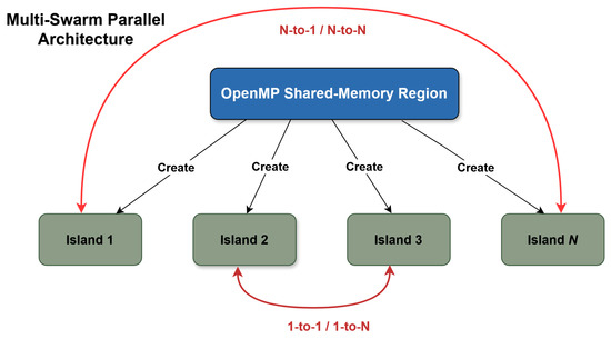
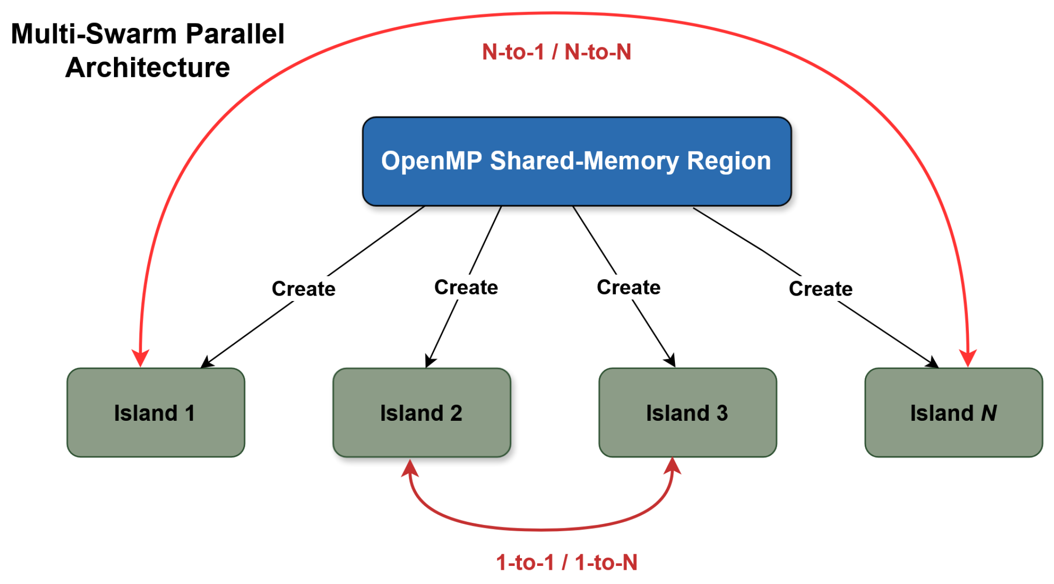
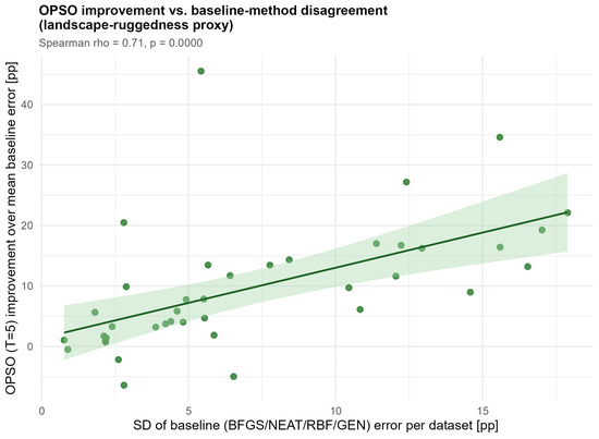
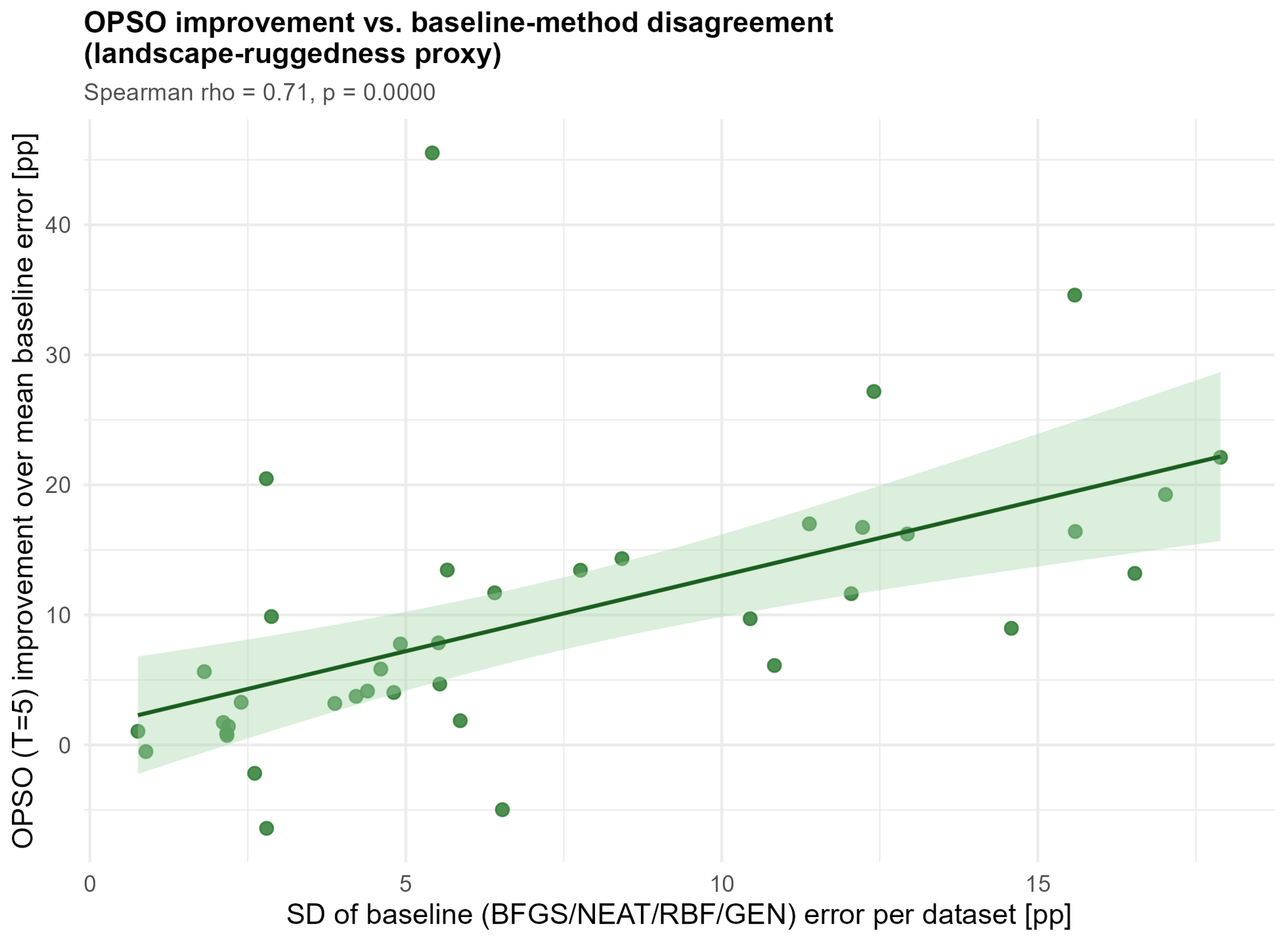
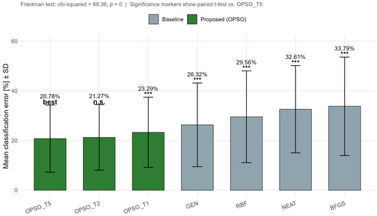
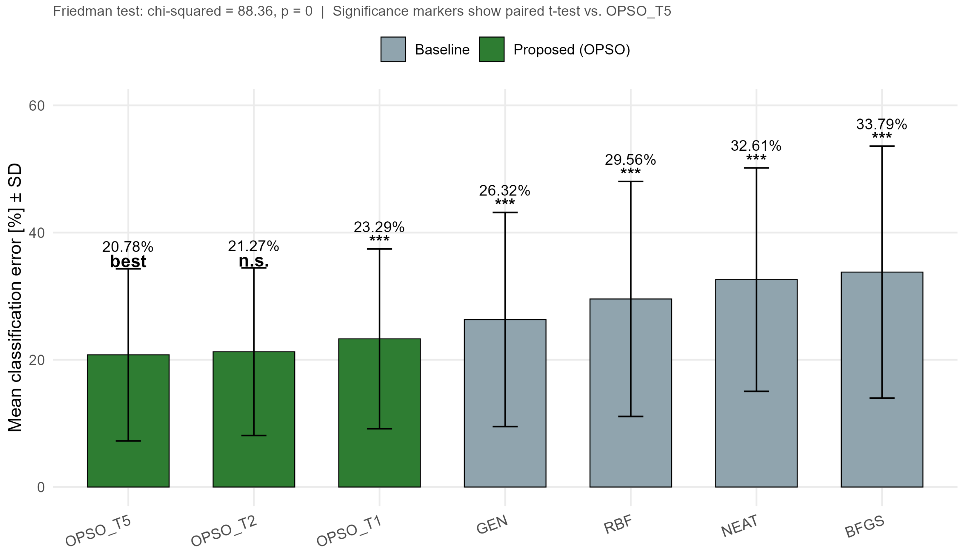
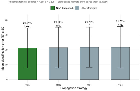
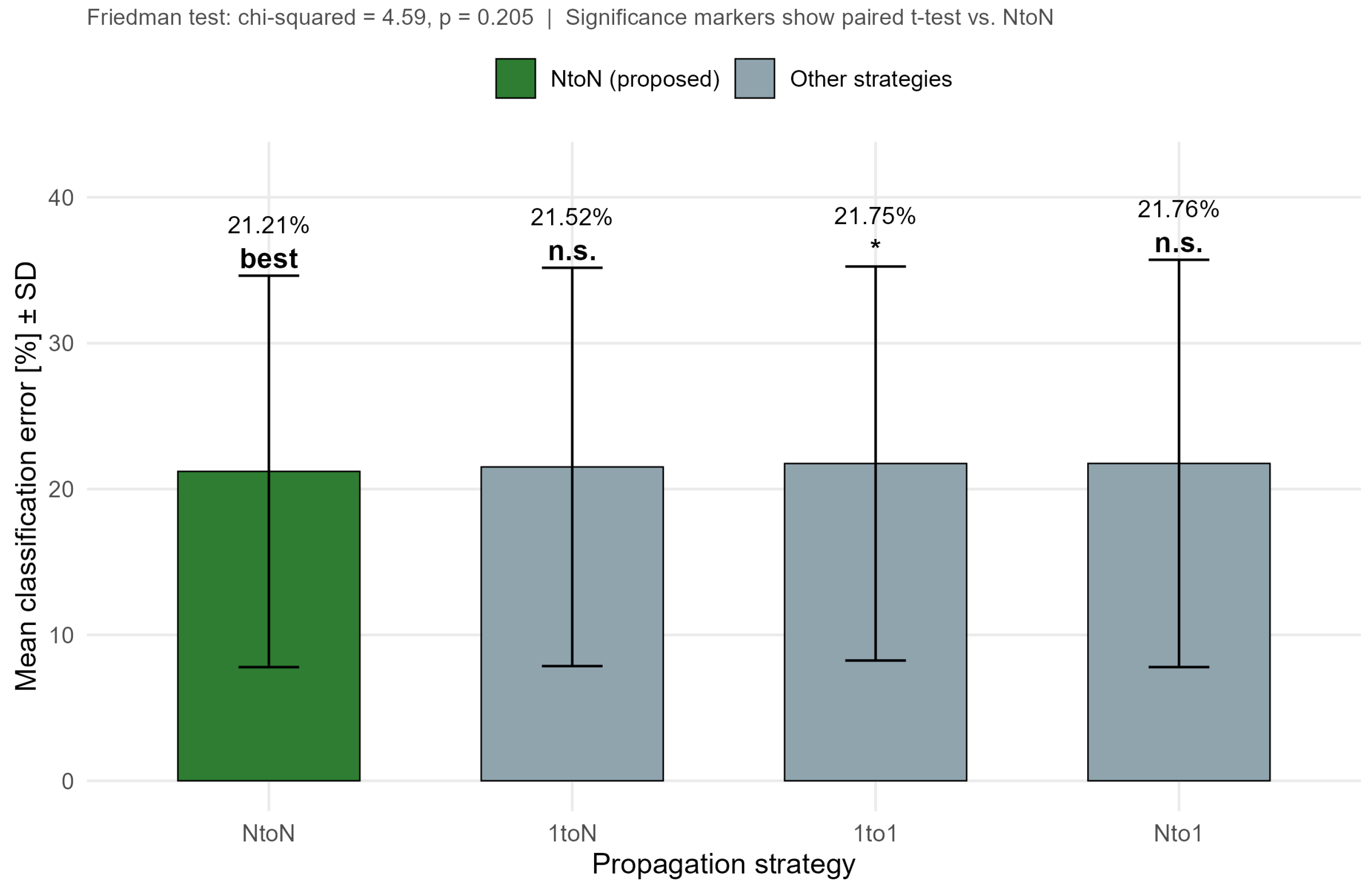
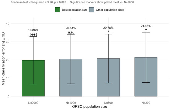

Disclaimer/Publisher’s Note: The statements, opinions and data contained in all publications are solely those of the individual author(s) and contributor(s) and not of MDPI and/or the editor(s). MDPI and/or the editor(s) disclaim responsibility for any injury to people or property resulting from any ideas, methods, instructions or products referred to in the content. |
© 2026 by the authors. Licensee MDPI, Basel, Switzerland. This article is an open access article distributed under the terms and conditions of the Creative Commons Attribution (CC BY) license.