Constrained Reinforcement Learning-Based Framework for DC Microgrid: Current Sharing and Voltage Regulation

Abstract

In this paper, a constrained reinforcement learning-based framework is developed for islanded DC microgrids to deal with the issues of voltage regulation and current sharing. First, a new local $\mathcal{Q}$ function including the current error and voltage error is designed on the basis of a hyperbolic function. The solution of the HJB equation associated with the local $\mathcal{Q}$ function yields an optimal policy. Then, a novel saturation-input policy iterative (SIPI) method is designed to approximate this policy. Its convergence is also analyzed in detail. To implement this SIPI method, an actor–critic control structure is developed, in which the actor network employs an asymmetric bounded function as its activation function to handle asymmetric input saturation. Finally, the effectiveness of the SIPI method is verified through numerical simulations.

1. Introduction

Recently, smart grids have become a prominent research topic. Researchers are increasingly focused on integrating cyber–physical techniques to enhance the intelligence of traditional power systems. Driven by advancements in computational intelligence and advanced control, highly distributed and autonomous power systems are rapidly evolving. Consequently, benefiting from their superior efficiency, reliability, and controllability over traditional AC systems, DC microgrids have drawn growing research interest [1,2,3,4]. Moreover, most renewable generations and terminal loads are inherently DC-based, which makes DC microgrids naturally compatible with them [5,6,7,8].

Current sharing and voltage regulation represent two fundamental operational challenges in islanded DC microgrids. Specifically, current sharing requires that the output currents of all sources be proportionally allocated according to their respective ratings, whereas voltage regulation demands that the common DC bus voltage settle precisely at the desired setpoint. To address these two problems, a diverse array of control strategies has been developed over the past decades [9,10,11,12,13,14,15,16,17,18,19,20,21,22,23,24]. Among these, the virtual output impedance technique, widely recognized as the V-I droop method, was first introduced in [9]. An inherent limitation of the conventional droop mechanism is its inability to simultaneously achieve precise voltage regulation and current sharing due to the fundamental trade-off between these two objectives. To circumvent this drawback, extensive research has been conducted within the hierarchical control framework, leading to two principal categories of enhanced approaches [10,11,12,13,14,15,16,17,18,19,20,21,22,23,24]. The first category centers on adaptive droop strategies, where the droop coefficients are dynamically tuned to refine current distribution accuracy [10,11,12,13,14,15]. Nevertheless, such approaches typically necessitate global load current information, which may be impractical to acquire. The second category focuses on augmenting the droop equation with additional feedback terms, thereby enhancing current-sharing performance through modified droop characteristics [16,17,18,19,20]. More recently, distributed consensus-based algorithms have gained considerable attention as an effective means of achieving current sharing within the hierarchical control architecture. Following this paradigm, analogous distributed coordination strategies have been successfully employed in [21,22,23,24,25,26,27].

From the perspective of computational intelligence, reinforcement learning (RL) provides an effective tool for addressing problems characterized by unknown model structures and parameters [28,29]. To date, mature RL-based techniques have been widely adopted in power systems, demonstrating significant efficacy in applications, e.g., stability enhancement and load frequency control (LFC) [30,31,32,33,34,35]. However, it can be seen that most of the existing studies were developed under the ideal assumption that the control inputs are unconstrained. In practical systems, the control inputs of DC–DC converters are inevitably subject to physical limitations such as actuator saturation, signal amplitude limits, and hardware protection thresholds, which are widely present to ensure safe and reliable operation under varying load conditions. Consequently, the applicability of the present algorithms in practice is rather limited.

To overcome this issue, this paper investigates a constrained reinforcement learning-based framework for islanded DC microgrids, which deals with the voltage regulation and current-sharing problems. The main contributions are summarized as follows:

(1)

A novel local $\mathcal{Q}$ function involving both the current error and the voltage error is constructed on the basis of a hyperbolic function. The solution of the resulting HJB equation then yields an optimal policy.

(2)

A new SIPI method is developed to obtain the optimal policy. Moreover, its convergence is established in detail.

(3)

To cope with asymmetric input saturation, the actor network employs an asymmetric bounded function as its activation function.

2. Preliminaries

2.1. Graph Theory

In the DC microgrid, each distributed generation unit is capable of exchanging information with its adjacent counterparts. The communication topology is modeled as a directed graph $G=\left({\Pi }_S,\mathcal{E},A\right)$, in which ${\Pi }_S$ represents the node set comprising all sources, $\mathcal{E}\subseteq {\Pi }_S\times {\Pi }_S$ denotes the edge set, and $A={(a_{ij})}_{M\times M}$ constitutes the weighted adjacency matrix. Whenever source j transmits information directly to source i, the corresponding entry satisfies $a_{ij}>0$; otherwise, $a_{ij}=0$. Moreover, self-loops are excluded by setting $a_{ii}=0$ for all i. Accordingly, the neighbor set of source i is defined by $N_i=\left\{j:\left(j,i\right)\in \mathcal{E}\right\}$. The graph Laplacian $L={(l_{ij})}_{M\times M}$ associated with G is formulated as $l_{ij}={\sum }_{k=1,k\ne i}^M{a}_{ik}$ if $i=j$, and $l_{ij}=-a_{ij}$ otherwise.

2.2. Model Description

This study considers an islanded DC microgrid consisting of M distributed generation units and N loads, where the sources are capable of bidirectional information exchange with neighboring units through a wide-area network (WAN). The set of generation sources is indexed by ${\Pi }_S=\left\{1,2\dots ,M\right\}$, whereas the load set is given by ${\Pi }_L=\left\{1,2\dots ,\mathrm{N}\right\}$. Each generation unit interfaces with the common DC bus through a boost-type DC/DC converter, while all loads are connected in a parallel configuration across the same bus. The common bus voltage is denoted by $V^{com}$. For the i-th source, $V_i$ and $I_i$ represent its terminal voltage and output current. The current-sharing objective for this DC microgrid is formally characterized as:

$${\displaystyle \frac{I_i}{d_i}}={\displaystyle \frac{I_j}{d_j}},for \forall i,j\in {\Pi }_S,$$

(1)

where $d_i$ stands for the sharing ratio.

The voltage regulation objective is formulated as:

$$V^{com}=V^{rated},$$

(2)

where $V^{rated}$ denotes the rated voltage for the DC bus.

2.3. Control Framework

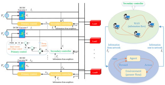
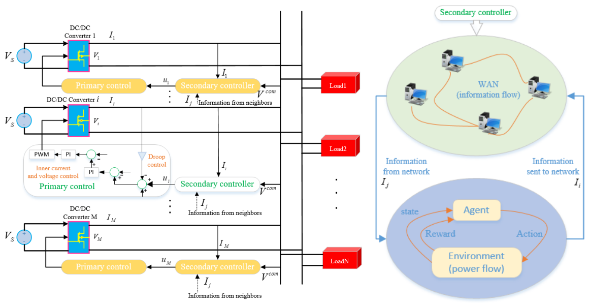
As illustrated in Figure 1, the adopted hierarchical control structure for each source comprises two cascaded layers: a primary control loop and a secondary control loop. By [21], the current-sharing controller is designed as:

$$\begin{array}{c}{V}_i^{Ref}(t)=V^{rated}-R_i^D{I}_i(t)+c_i(t),\hfill \\ {\dot{c}}_i(t)=u_i(t),\hfill \end{array}$$

(3)

where $V_i^{Ref}$ is the desired reference, $R_i^D$ denotes a virtual resistance, and $u_i$ represents the control input.

Figure 1. Hierarchical control framework for an islanded DC microgrid.

Let $\{t_1,t_2,\dots \}$ denote the sampling instants satisfying $t_{\sigma +1}-t_{\sigma }=h$, with $h>0$ being the sampling period. Here, the virtual resistance is chosen as $R_i^D=0$. Owing to the fast dynamics of the voltage loops and inner current, the converter output voltage $V_i$ rapidly tracks its reference $V_i^{Ref}$ within each interval h. Hence, we can derive that $V_i(t_{\sigma })=V_i^{Ref}(t_{\sigma })$. Let $V_i(\sigma )=V_i(t_{\sigma })$. Then, we have

$$\begin{array}{c}{V}_i(\sigma )=V^{rated}+c_i(\sigma ),\hfill \\ c_i(\sigma +1)=c_i(\sigma )+h\ast u_i(\sigma ),\hfill \end{array}$$

(4)

where $u_i(\sigma )$ denotes the control input at time $t_{\sigma }$. In practical DC microgrids, owing to the finite modulation index and limited voltage regulation margins of power electronic interfaces, the input $u_i(\sigma )$ is inherently bounded by physical actuator constraints. The control constraint is specifically described as follows:

$$\begin{array}{c}\hfill u_i=\left\{\begin{array}{cc}{\overline{u}}_i,\hspace{0.5em}\hfill & u_i>{\overline{u}}_i,\hfill \\ u_i,\hspace{0.5em}\hfill & {\underline{u}}_i\le u_i\le {\overline{u}}_i\hfill \\ {\underline{u}}_i,\hspace{0.5em}\hfill & u_i<{\underline{u}}_i,\hfill \end{array}\right.,\end{array}$$

(5)

where ${\overline{u}}_i>0$ and ${\underline{u}}_i<0$ denote the upper and lower bounds of the constrained actuator, respectively.

Let $R_i^L$ represent the ith load’s constant resistance. By [21], the dynamics of the DC microgrid are described as:

$$V^{com}={\displaystyle \frac{1}{{\sum }_{i\in {\Pi }_S}{G}_i+{\sum }_{i\in {\Pi }_L}(1/R_i^L)}}\sum _{i\in {\Pi }_S}{G}_i(V_i),$$

(6)

$$I_i=G_i(V_i-V^{com}),$$

(7)

where $G_i$ denotes the conductance of the transmission line between the ith converter and the DC bus.

2.4. Problem Formulation

Based on (1) and (2), ${\chi }_V(\sigma )$ and ${\chi }_{I,i}(\sigma )$ are defined as

$${\chi }_V(\sigma )=V^{com}(\sigma )-V^{rated},$$

(8)

$${\chi }_{I,i}(\sigma )=\sum _{j\in N_i}{a}_{ij}\left({\displaystyle \frac{I_j(\sigma )}{d_j}}-{\displaystyle \frac{I_i(\sigma )}{d_i}}\right),$$

(9)

where ${\chi }_V$ and ${\chi }_{I,i}$ denote the voltage error and current error, respectively. By (9), one obtains ${\chi }_I(\sigma )=-L{D}^{-1}I(\sigma )$, where L stands for the Laplacian matrix and $D=diag\{d_1,\dots ,d_N\}$ represents the diagonal matrix of sharing ratios. The null space of $L{D}^{-1}$ is spanned by the vector ${[d_1,d_2,\dots ,d_N]}^T$ if and only if G is connected.

By (6)–(9), one can obtain

$${\chi }_V(\sigma +1)={\chi }_V(\sigma )+\lambda h\sum _{i\in {\Pi }_S}(G_i(u_i(\sigma ))),$$

(10)

$$\begin{array}{c}\hfill {\chi }_{I,i}(\sigma +1)=h{ƛ}_i{G}_i{u}_i(\sigma )+{\chi }_{I,i}(\sigma )+h\sum _{j\in N_i}{a}_{ij}{\displaystyle \frac{G_j{u}_j(\sigma )}{d_j}}\hfill \\ \hfill +h\lambda {\displaystyle \sum _{j\in N_i}}{\displaystyle \frac{a_{ij}}{d_j}}{\displaystyle \sum _{l\in {\Pi }_S/\{i\}}}{G}_l{u}_l(\sigma )\hfill \end{array},$$

(11)

where ${ƛ}_i=\left({\displaystyle \frac{l_{ii}(\lambda -1)}{d_i}}-{\sum }_{j\in N_i}{\displaystyle \frac{\lambda a_{ij}}{d_j}}\right)$ with $\lambda ={\displaystyle \frac{1}{{\sum }_{i\in {\Pi }_S}{G}_i+{\sum }_{i\in {\Pi }_L}(1/R_i^L)}}$.

Define $u_{-i}(\sigma )\triangleq \{u_j(\sigma ):j\in {\Pi }_S,j\ne i\}$ as the control actions of all sources except source i. For each source i, the local performance function is designed as

$$\begin{array}{cc}\hfill & J_i(\sigma )\hfill \\ \hfill & ={\displaystyle \sum _{\tau =\sigma }^{\infty }}{\gamma }^{\tau -\sigma }{\psi }_i({\chi }_{I,i}(\sigma ),{\chi }_V(\sigma ),u_i(\sigma ),u_{-i}(\sigma )),\hfill \\ \hfill & ={\displaystyle \sum _{\tau =\sigma }^{\infty }}{\gamma }^{\tau -\sigma }\left(\aleph {\chi }_{I,i}^2(\tau )+\hslash {\chi }_V^2(\tau )+\mathcal{S}(u_i(\tau ))+\sum _{j\in {\Pi }_S/\{i\}}\mathcal{S}(u_j(\tau ))\right).\hfill \end{array}$$

(12)

where $0<\gamma \le 1$ denotes the discount factor, $\aleph >0$ and $\hslash >0$. $\mathcal{S}(u_i(\sigma ))$ is designed as

$$\begin{array}{c}\hfill \mathcal{S}(u_i)=2{\int }_0^{u_i}{\overline{u}}_i{\zeta }_i^{-1}({\omega }_i)d{\omega }_i\end{array},$$

where ${\zeta }_i$ is designed as

$$\begin{array}{c}\hfill {\zeta }_i({\omega }_i)={\displaystyle \frac{e^{{\omega }_i}-e^{-{\omega }_i}}{\frac{1}{{\overline{u}}_i}{e}^{{\omega }_i}-\frac{1}{{\underline{u}}_i}{e}^{-{\omega }_i}}}\end{array}.$$

Definition 1.

For $\forall i\in {\Pi }_S$, the constrained control $u_i(\sigma )$ is considered to be admissible if it satisfies the following conditions: (1) $u_i(\sigma )$ is continuous on ${\Omega }_u$; (2) $u_i(\sigma )$ can stabilize the error systems (8) and (9); and (3) $u_i(\sigma )$ can guarantee (12) is finite, i.e., $J_i(0)={\sum }_{\tau =0}^{\infty }{\gamma }^{\tau }{\psi }_i({\chi }_{I,i}(\tau ),{\chi }_V(\tau ),u_i(\tau ),u_{-i}(\tau ))<+\infty$, where $0<\gamma \le 1$.

Definition 2.

For the N-player dynamic graphical game, an N-tuple of optimal control policies $\{u_1^{\ast },u_2^{\ast },\dots ,u_N^{\ast }\}$ constitutes a Nash equilibrium solution if, for all $i\in N$,

$$\begin{array}{c}\hfill J_i^{\ast }\equiv J_i(u_i^{\ast },u_{-i}^{\ast })\le J_i(u_i,u_{-i}^{\ast }).\end{array}$$

(13)

The N-tuple $\{J_1^{\ast },J_2^{\ast },\dots ,J_N^{\ast }\}$ is called the Nash equilibrium outcome of the N-player game.

Problem 1.

This paper aims to develop a controller for each source such that (1) and (2) are achieved, and meanwhile, each source’s local performance is minimized; that is, the control $u_i(\sigma )$ not only minimizes the local performance index $J_i$, but also makes (8) and (9) stable.

Given a fixed admissible control $u_i(\sigma )$, we define the $\mathcal{Q}$ function ${\mathcal{Q}}_i$ as

$$\begin{array}{cc}\hfill & {\mathcal{Q}}_i({\chi }_{I,i}(\sigma ),{\chi }_V(\sigma ),u_i(\sigma ),u_{-i}(\sigma ))\hfill \\ \hfill & ={\displaystyle \sum _{\tau =\sigma }^{\infty }}{\gamma }^{\tau -\sigma }\left(\aleph {\chi }_{I,i}^2(\tau )+\hslash {\chi }_V^2(\tau )+\mathcal{S}(u_i(\tau ))+\sum _{j\in {\Pi }_S/\{i\}}\mathcal{S}(u_j(\tau ))\right).\hfill \end{array}$$

According to Bellman’s optimality principle, one has

$$\begin{array}{cc}\hfill & {\mathcal{Q}}_i^{\ast }({\chi }_{I,i}(\sigma ),{\chi }_V(\sigma ),u_i^{\ast }(\sigma ),u_{-i}^{\ast }(\sigma ))\hfill \\ \hfill & ={\psi }_i({\chi }_{I,i}(\sigma ),{\chi }_V(\sigma ),u_i^{\ast }(\sigma ),u_{-i}^{\ast }(\sigma ))\hfill \\ \hfill & +\gamma {\mathcal{Q}}_i^{\ast }({\chi }_{I,i}(\sigma +1),{\chi }_V(\sigma +1),u_i^{\ast }(\sigma +1)),\hfill \end{array}$$

(14)

where $u_i^{\ast }$ is the optimal constrained policy and ${\mathcal{Q}}_i^{\ast }$ is the optimal $\mathcal{Q}$ function. Using Bellman’s optimality principle, (14) admits the following equivalent form:

$$\begin{array}{cc}\hfill & {\mathcal{Q}}_i^{\ast }({\chi }_{I,i}(\sigma ),{\chi }_V(\sigma ),u_i^{\ast }(\sigma ),u_{-i}^{\ast }(\sigma ))\hfill \\ \hfill & =\underset{u_i(\sigma )}{\min }\{{\psi }_i({\chi }_{I,i}(\sigma ),{\chi }_V(\sigma ),u_i(\sigma ),u_{-i}(\sigma ))\hfill \\ \hfill & +\gamma {\mathcal{Q}}_i^{\ast }({\chi }_{I,i}(\sigma +1),{\chi }_V(\sigma +1),u_i^{\ast }(\sigma +1),u_{-i}^{\ast }(\sigma +1))\}.\hfill \end{array}$$

(15)

By (15), $u_i^{\ast }$ is

$$\begin{array}{cc}\hfill u_i^{\ast }(\sigma )& =\arg \underset{u_i}{\min }\{{\psi }_i({\chi }_{I,i}(\sigma ),{\chi }_V(\sigma ),u_i(\sigma ),u_{-i}(\sigma ))\hfill \\ \hfill & +\gamma {\mathcal{Q}}_i^{\ast }({\chi }_{I,i}(\sigma +1),{\chi }_V(\sigma +1),u_i^{\ast }(\sigma +1),u_{-i}^{\ast }(\sigma +1))\}.\hfill \end{array}$$

(16)

Differentiating ${\mathcal{Q}}_i$ with respect to $u_i(\sigma )$ in (15) yields

$$u_i^{\ast }(\sigma )={\zeta }_i(-{\displaystyle \frac{h{G}_i\gamma }{2{\overline{u}}_i}}({ƛ}_i{\displaystyle \frac{\partial {\mathcal{Q}}_i^{\ast }}{\partial {\chi }_{I,i}(\sigma +1)}}+\lambda {\displaystyle \frac{\partial {\mathcal{Q}}_i^{\ast }}{\partial {\chi }_V(\sigma +1)}})),$$

(17)

where ${\mathcal{Q}}_i^{\ast }={\mathcal{Q}}_i^{\ast }({\chi }_{I,i}(\sigma +1),{\chi }_V(\sigma +1),u_i^{\ast }(\sigma +1),u_{-i}^{\ast }(\sigma +1))$.

Lemma 1.

Suppose ${\mathcal{Q}}_i^{\ast }$ satisfies (14), then the policies given by (17) can ensure the following results:

(1) 

Both current sharing (1) and voltage regulation (2) are realized.

(2) 

The Nash equilibrium for the current-sharing problem is guaranteed.

Proof. 

Consider the following Lyapunov function:

$$Z_i(\sigma )={\gamma }^{\sigma }{\mathcal{Q}}_i^{\ast }({\chi }_{I,i}(\sigma ),{\chi }_V(\sigma ),u_i^{\ast }(\sigma ),u_{-i}^{\ast }(\sigma )).$$

(18)

Since ${\mathcal{Q}}_i^{\ast }$ satisfies Bellman’s optimality principle (14), one can obtain

$$\begin{array}{cc}\hfill & Z_i(\sigma +1)-Z_i(\sigma )\hfill \\ \hfill & ={\gamma }^{\sigma +1}{\mathcal{Q}}_i^{\ast }({\chi }_{I,i}(\sigma +1),{\chi }_V(\sigma +1),u_i^{\ast }(\sigma +1),u_{-i}^{\ast }(\sigma +1))\hfill \\ \hfill & -{\gamma }^{\sigma }{\mathcal{Q}}_i^{\ast }({\chi }_{I,i}(\sigma ),{\chi }_V(\sigma ),u_i^{\ast }(\sigma ),u_{-i}^{\ast }(\sigma ))\hfill \\ \hfill & =- {\gamma }^{\sigma } {\psi }_i({\chi }_{I,i}(\sigma ),{\chi }_V(\sigma ),u_i^{\ast }(\sigma ),u_{-i}^{\ast }(\sigma ))\le 0.\hfill \end{array}$$

(19)

Note that $Z_i(\sigma )=0$ only when ${\mathcal{Q}}_i^{\ast }=0$, which suggests that ${\chi }_{I,i}=0$ and ${\chi }_V=0$. From (19), $Z_i(\sigma )$ is decreasing, which means that ${\chi }_{I,i}(\sigma )$ and ${\chi }_V(\sigma )$ are asymptotically stable. Thereby, both current sharing in (1) and voltage regulation in (2) are implemented.

From the above, and for $\forall i\in {\Pi }_S$, $u_i^{\ast }$ is an admissible control, so we have

$$J_i^{\ast }={\mathcal{Q}}_i^{\ast }({\chi }_{I,i}(0),{\chi }_V(0),u_i^{\ast },u_{-i}^{\ast })<+\infty .$$

(20)

We know that $u_i(\sigma )$ is an admissible control and the performance index under $u_i(\sigma )$ is ${\mathcal{Q}}_i({\chi }_{I,i}(\sigma ),{\chi }_V(\sigma ),u_i(\sigma ))$ for $\forall i\in {\Pi }_S$. Then, according to Bellman’s optimality principle, there exists

$${\mathcal{Q}}_i^{\ast }({\chi }_{I,i}(\sigma ),{\chi }_V(\sigma ),u_i^{\ast }(\sigma ),u_{-i}^{\ast }(\sigma ))\le {\mathcal{Q}}_i({\chi }_{I,i}(\sigma ),{\chi }_V(\sigma ),u_i(\sigma ),u_{-i}^{\ast }(\sigma )),$$

(21)

which indicates that $J_i^{\ast }(u_i^{\ast },u_{-i}^{\ast })\le J_i(u_i,u_{-i}^{\ast })$. Therefore, the Nash equilibrium is guaranteed and Problem 1 is solved. The proof is completed. □

Remark 1.

The existing works [30,31,32,33,34,35] all use RL algorithms in DC microgrid control, and do not consider the control upper and lower bounds. The absence of upper and lower bounds can cause the system input to exceed the system threshold and cause a failure. To solve this problem, this paper proposes an RL control algorithm with constraints. The control input is constrained and asymmetric.

Remark 2.

A series of constrained RL methods were proposed using hyperbolic function $\tanh (·)$ for symmetric input constraints [36,37,38]. To tackle asymmetric control bounds, this paper designs a novel cost function by selecting ${\zeta }_i({\omega }_i)={\displaystyle \frac{e^{{\omega }_i}-e^{-{\omega }_i}}{\frac{1}{{\overline{u}}_i}{e}^{{\omega }_i}-\frac{1}{{\underline{u}}_i}{e}^{-{\omega }_i}}}$, so that the resulting optimal constrained control law is fundamentally different from those reported in the existing works [36,37,38].

Remark 3.

Note that under an admissible control (Definition 1), the infinite-horizon sum in (12) remains bounded even for $\gamma =1$: the convergence of the series requires ${\psi }_i({\chi }_{I,i}(\sigma ),{\chi }_V(\sigma ),u_i(\sigma ),u_{-i}(\sigma ))\to 0$ as $\sigma \to \infty$, which, by the positive definiteness of ${\psi }_i$, implies that the local cost vanishes under admissible policies.

3. Current-Sharing Scheme

3.1. Saturation-Input Policy Iterative Algorithm (SIPI)

In this subsection, the SIPI algorithm is summarized in Algorithm 1.

Algorithm 1 The saturation-input policy iteration (SIPI) algorithm

Initialization: Initialize an admissible control law $u_i^{(0)}(\sigma )$. Compute ${\mathcal{Q}}_i^{(0)}({\chi }_{I,i}(\sigma ),{\chi }_V(\sigma ),u_i^{(0)}(\sigma ),u_{-i}^{(0)}(\sigma ))$: $$\begin{array}{cc}\hfill & {\mathcal{Q}}_i^{(0)}({\chi }_{I,i}(\sigma ),{\chi }_V(\sigma ),u_i^{(0)}(\sigma ),u_{-i}^{(0)}(\sigma ))\hfill \\ \hfill =& {\psi }_i({\chi }_{I,i}(\sigma ),{\chi }_V(\sigma ),u_i^{(0)}(\sigma ),u_{-i}^{(0)}(\sigma ))\hfill \\ \hfill & +\gamma {\mathcal{Q}}_i^{(0)}({\chi }_{I,i}(\sigma +1),{\chi }_V(\sigma +1),u_i^{(0)}(\sigma +1),u_{-i}^{(0)}(\sigma +1)).\hfill \end{array}$$ Update $u_i^{(1)}(\sigma )$ as: $$\begin{array}{cc}\hfill u_i^{(1)}(\sigma )=& \arg \underset{u_i(\sigma )}{\min }({\psi }_i({\chi }_{I,i}(\sigma ),{\chi }_V(\sigma ),u_i(\sigma ),u_{-i}(\sigma ))\hfill \\ \hfill & +\gamma {\mathcal{Q}}_i^{(0)}({\chi }_{I,i}(\sigma +1),{\chi }_V(\sigma +1),u_i^{(0)}(\sigma +1),u_{-i}^{(0)}(\sigma +1))).\hfill \end{array}$$ Let $d=1$. Iteration: Step 1: Compute ${\mathcal{Q}}_i^{(d)}({\chi }_{I,i}(\sigma ),{\chi }_V(\sigma ),u_i^{(d)}(\sigma ),u_{-i}^{(d)}(\sigma ))$ as $$\begin{array}{cc}\hfill & {\mathcal{Q}}_i^{(d)}({\chi }_{I,i}(\sigma ),{\chi }_V(\sigma ),u_i^{(d)}(\sigma ),u_{-i}^{(d)}(\sigma ))\hfill \\ \hfill =& {\psi }_i({\chi }_{I,i}(\sigma ),{\chi }_V(\sigma ),u_i^{(d)}(\sigma ),u_{-i}^{(d)}(\sigma ))\hfill \\ \hfill & +\gamma {\mathcal{Q}}_i^{(d)}({\chi }_{I,i}(\sigma +1),{\chi }_V(\sigma +1),u_i^{(d)}(\sigma +1),u_{-i}^{(d)}(\sigma +1)).\hfill \end{array}$$ (22) Step 2: Update $u_i^{(d+1)}(\sigma )$ as $$\begin{array}{cc}\hfill u_i^{(d+1)}(\sigma )=& \arg \underset{u_i(\sigma )}{\min }({\psi }_i({\chi }_{I,i}(\sigma ),{\chi }_V(\sigma ),u_i(\sigma ),u_{-i}(\sigma ))\hfill \\ \hfill & +\gamma {\mathcal{Q}}_i^{(d)}({\chi }_{I,i}(\sigma +1),{\chi }_V(\sigma +1),u_i^{(d)}(\sigma +1),u_{-i}^{(d)}(\sigma +1))).\hfill \end{array}$$ (23) Step 3: If ${\mathcal{Q}}_i^{(d)}$ converges to ${\mathcal{Q}}_i^{\ast }$, break; else $d=d+1$, go to Step 1.

3.2. Convergence Analysis

Throughout the SIPI algorithm, each source updates its policy by (23), with the other sources’ policies held fixed at their current iterates $u_{-i}^{(d)}(\sigma )$, i.e., the iteration is a simultaneous best-response iteration. Then, for the subsequent convergence analysis, we need the following Lemmas and Assumption.

Lemma 2

([39,40]). For $\forall i$ and $\forall d$;, if initial policy $u_i^{(0)}(\sigma )$ is admissible, then $u_i^{(d)}(\sigma )$ is still admissible, i.e., $u_i^{(d)}(\sigma )$ both creates an error (8) and makes the system stable (9), guaranteeing that the performance function (12) is finite.

Assumption 1

([41]). Let $\mathcal{T}$ denote the joint best-response operator that maps the current joint policy profile $u^{(d)}={\{u_i^{(d)}\}}_{i\in {\Pi }_S}$ to the updated profile $u^{(d+1)}={\{u_i^{(d+1)}\}}_{i\in {\Pi }_S}$ generated by (23). There exists a constant $\rho \in (0,1)$ such that, for any two admissible joint policy profiles u and $u^{\prime }$,

$$\parallel \mathcal{T}(u)-\mathcal{T}(u^{\prime })\parallel \le \rho \parallel u-u^{\prime }\parallel ,$$

where $\parallel u\parallel \triangleq {\max }_{i\in {\Pi }_S}{\sup }_{\sigma }\left|u_i(\sigma )\right|$.

In what follows, $Q_i({\chi }_{I,i},{\chi }_V,u_i,u_{-i})$ denotes the value function under an arbitrary admissible joint policy profile $(u_i,u_{-i})$, and $Q_i^{(d)}({\chi }_{I,i},{\chi }_V)\triangleq Q_i({\chi }_{I,i},{\chi }_V,u_i^{(d)},u_{-i}^{(d)})$ denotes its shorthand under the d-th iterate.

Lemma 3.

For $\forall i$ and $\forall d\ge 1$, if $u_i^{(d)}(\sigma )$ is admissible, then the policy improvement step (23), with the other sources’ policies held fixed at $u_{-i}^{(d)}(\sigma )$, yields a non-increasing value, i.e.,

$${\mathcal{Q}}_i({\chi }_{I,i}(\sigma ),{\chi }_V(\sigma ),u_i^{(d+1)}(\sigma ),u_{-i}^{(d)}(\sigma ))\le {\mathcal{Q}}_i^{(d)}({\chi }_{I,i}(\sigma ),{\chi }_V(\sigma ),u_i^{(d)}(\sigma ),u_{-i}^{(d)}(\sigma )).$$

Proof. 

First, we define a new value function ${\mathrm{P}}_i^{(d+1)}({\chi }_{I,i}(\sigma ),{\chi }_V(\sigma ),u_i^{(d+1)}(\sigma ),u_{-i}^{(d)}(\sigma ))$ as follows:

$$\begin{array}{cc}\hfill & {\mathrm{P}}_i^{(d+1)}({\chi }_{I,i}(\sigma ),{\chi }_V(\sigma ),u_i^{(d+1)}(\sigma ),u_{-i}^{(d)}(\sigma ))\hfill \\ \hfill & \triangleq {\psi }_i({\chi }_{I,i}(\sigma ),{\chi }_V(\sigma ),u_i^{(d+1)}(\sigma ),u_{-i}^{(d)}(\sigma ))\hfill \\ \hfill & +\gamma {\mathcal{Q}}_i^{(d)}({\chi }_{I,i}(\sigma +1),{\chi }_V(\sigma +1),u_i^{(d)}(\sigma +1),u_{-i}^{(d)}(\sigma +1))\hfill \\ \hfill & =\underset{u_i(\sigma )}{\min }({\psi }_i({\chi }_{I,i}(\sigma ),{\chi }_V(\sigma ),u_i(\sigma ),u_{-i}^{(d)}(\sigma ))\hfill \\ \hfill & +\gamma {\mathcal{Q}}_i^{(d)}({\chi }_{I,i}(\sigma +1),{\chi }_V(\sigma +1),u_i^{(d)}(\sigma +1),u_{-i}^{(d)}(\sigma +1))).\hfill \end{array}$$

(24)

According to (22) and (24), one has

$$\begin{array}{cc}\hfill & {\mathrm{P}}_i^{(d+1)}({\chi }_{I,i}(\sigma ),{\chi }_V(\sigma ),u_i^{(d+1)}(\sigma ),u_{-i}^{(d)}(\sigma ))\hfill \\ \hfill & \le {\mathcal{Q}}_i^{(d)}({\chi }_{I,i}(\sigma ),{\chi }_V(\sigma ),u_i^{(d)}(\sigma ),u_{-i}^{(d)}(\sigma )).\hfill \end{array}$$

(25)

According to Lemma 2, since $u_i^{(d)}(\sigma )$ is admissible, one has ${\chi }_V(\sigma )\to 0$ and ${\chi }_{I,i}(\sigma )\to 0$ when $\sigma \to \infty$. Let $\sigma =\mathcal{F}$, where $\mathcal{F}\to \infty$, so that one has

$$\begin{array}{cc}\hfill & {\mathcal{Q}}_i({\chi }_{I,i}(\mathcal{F}),{\chi }_V(\mathcal{F}),u_i^{(d+1)}(\mathcal{F}),u_{-i}^{(d)}(\mathcal{F}))\hfill \\ \hfill & ={\mathrm{P}}_i^{(d+1)}({\chi }_{I,i}(\mathcal{F}),{\chi }_V(\mathcal{F}),u_i^{(d+1)}(\mathcal{F}),u_{-i}^{(d)}(\mathcal{F}))\hfill \\ \hfill & = {\mathcal{Q}}_i^{(d)}({\chi }_{I,i}(\mathcal{F}),{\chi }_V(\mathcal{F}),u_i^{(d)}(\mathcal{F}),u_{-i}^{(d)}(\mathcal{F})).\hfill \end{array}$$

(26)

Let $\sigma =\mathcal{F}-1$. From (22), (23), and (26), one has

$$\begin{array}{cc}\hfill & {\mathcal{Q}}_i({\chi }_{I,i}(\mathcal{F}-1),{\chi }_V(\mathcal{F}-1),u_i^{(d+1)}(\mathcal{F}-1),u_{-i}^{(d)}(\mathcal{F}-1))\hfill \\ \hfill & ={\psi }_i({\chi }_{I,i}(\mathcal{F}-1),{\chi }_V(\mathcal{F}-1),u_i^{(d+1)}(\mathcal{F}-1),u_{-i}^{(d)}(\mathcal{F}-1))\hfill \\ \hfill & +\gamma {\mathcal{Q}}_i({\chi }_{I,i}(\mathcal{F}),{\chi }_V(\mathcal{F}),u_i^{(d+1)}(\mathcal{F}),u_{-i}^{(d)}(\mathcal{F}))\hfill \\ \hfill & ={\psi }_i({\chi }_{I,i}(\mathcal{F}-1),{\chi }_V(\mathcal{F}-1),u_i^{(d+1)}(\mathcal{F}-1),u_{-i}^{(d)}(\mathcal{F}-1))\hfill \\ \hfill & +\gamma {\mathcal{Q}}_i^{(d)}({\chi }_{I,i}(\mathcal{F}),{\chi }_V(\mathcal{F}),u_i^{(d)}(\mathcal{F}),u_{-i}^{(d)}(\mathcal{F}))\hfill \\ \hfill & =\underset{u_i(\mathcal{F}-1)}{\min }({\psi }_i({\chi }_{I,i}(\mathcal{F}-1),{\chi }_V(\mathcal{F}-1),u_i(\mathcal{F}-1),u_{-i}^{(d)}(\mathcal{F}-1))\hfill \\ \hfill & +\gamma {\mathcal{Q}}_i^{(d)}({\chi }_{I,i}(\mathcal{F}),{\chi }_V(\mathcal{F}),u_i^{(d)}(\mathcal{F}),u_{-i}^{(d)}(\mathcal{F}))\hfill \\ \hfill & \le {\psi }_i({\chi }_{I,i}(\mathcal{F}-1),{\chi }_V(\mathcal{F}-1),u_i^{(d)}(\mathcal{F}-1),u_{-i}^{(d)}(\mathcal{F}-1))\hfill \\ \hfill & +\gamma {\mathcal{Q}}_i^{(d)}({\chi }_{I,i}(\mathcal{F}),{\chi }_V(\mathcal{F}),u_i^{(d)}(\mathcal{F}),u_{-i}^{(d)}(\mathcal{F})))\hfill \\ \hfill & ={\mathcal{Q}}_i^{(d)}({\chi }_{I,i}(\mathcal{F}-1),{\chi }_V(\mathcal{F}-1),u_i^{(d)}(\mathcal{F}-1),u_{-i}^{(d)}(\mathcal{F}-1)).\hfill \end{array}$$

(27)

From (27), ${\mathcal{Q}}_i({\chi }_{I,i}(\sigma ),{\chi }_V(\sigma ),u_i^{(d+1)}(\sigma ),u_{-i}^{(d)}(\sigma ))\le {\mathcal{Q}}_i^{(d)}({\chi }_{I,i}(\sigma ),{\chi }_V(\sigma ),u_i^{(d)}(\sigma ),u_{-i}^{(d)}(\sigma ))$ when $\sigma =\mathcal{F}-1$. Let $\sigma =\mathcal{A}+1$, where $\mathcal{A}=0,1,2,\cdots$, so that one has ${\mathcal{Q}}_i({\chi }_{I,i}(\mathcal{A}+1),{\chi }_V(\mathcal{A}+1),u_i^{(d+1)}(\mathcal{A}+1),u_{-i}^{(d)}(\mathcal{A}+1))\le {\mathcal{Q}}_i^{(d)}({\chi }_{I,i}(\mathcal{A}+1),{\chi }_V(\mathcal{A}+1),u_i^{(d)}(\mathcal{A}+1)$, $u_{-i}^{(d)}(\mathcal{A}+1))$. Let $\sigma =\mathcal{A}$, then we can obtain

$$\begin{array}{cc}\hfill & {\mathcal{Q}}_i({\chi }_{I,i}(\mathcal{A}),{\chi }_V(\mathcal{A}),u_i^{(d+1)}(\mathcal{A}),u_{-i}^{(d)}(\mathcal{A}))\hfill \\ \hfill & ={\psi }_i({\chi }_{I,i}(\mathcal{A}),{\chi }_V(\mathcal{A}),u_i^{(d+1)}(\mathcal{A}),u_{-i}^{(d)}(\mathcal{A}))\hfill \\ \hfill & +\gamma {\mathcal{Q}}_i({\chi }_{I,i}(\mathcal{A}+1),{\chi }_V(\mathcal{A}+1),u_i^{(d+1)}(\mathcal{A}+1),u_{-i}^{(d)}(\mathcal{A}+1))\hfill \\ \hfill & \le {\psi }_i({\chi }_{I,i}(\mathcal{A}),{\chi }_V(\mathcal{A}),u_i^{(d+1)}(\mathcal{A}),u_{-i}^{(d)}(\mathcal{A}))\hfill \\ \hfill & +\gamma {\mathcal{Q}}_i^{(d)}({\chi }_{I,i}(\mathcal{A}+1),{\chi }_V(\mathcal{A}+1),u_i^{(d)}(\mathcal{A}+1),u_{-i}^{(d)}(\mathcal{A}+1))\hfill \\ \hfill & =P_i^{(d+1)}({\chi }_{I,i}(\mathcal{A}),{\chi }_V(\mathcal{A}),u_i^{(d+1)}(\mathcal{A}),u_{-i}^{(d)}(\mathcal{A}))\hfill \\ \hfill & \le {\mathcal{Q}}_i^{(d)}({\chi }_{I,i}(\mathcal{A}),{\chi }_V(\mathcal{A}),u_i^{(d)}(\mathcal{A}),u_{-i}^{(d)}(\mathcal{A})).\hfill \end{array}$$

(28)

According to (28), one has ${\mathcal{Q}}_i({\chi }_{I,i}(\sigma ),{\chi }_V(\sigma ),u_i^{(d+1)}(\sigma ),u_{-i}^{(d)}(\sigma ))\le {\mathcal{Q}}_i^{(d)}({\chi }_{I,i}(\sigma ),{\chi }_V(\sigma ),$$u_i^{(d)}(\sigma ),u_{-i}^{(d)}(\sigma ))$ for $\forall d$ and $\forall i$. This completes the proof. □

Theorem 1.

Under Assumption 1, for any admissible initial joint policy profile $u^{(0)}$, the sequence $\{u^{(d)}\}$ generated by the simultaneous best-response iteration (22)–(23) converges to the unique fixed point $u^{\ast }={\{u_i^{\ast }\}}_{i\in {\Pi }_S}$ of $\mathcal{T}$, and ${\mathcal{Q}}_i^{(d)}$ converges to ${\mathcal{Q}}_i^{\ast }$, satisfying (14). Moreover, by Lemma 1, $u^{\ast }$ constitutes the Nash equilibrium.

Proof. 

By Assumption 1, one has

$$\parallel u^{(d+1)}-u^{(d)}\parallel =\parallel \mathcal{T}(u^{(d)})-\mathcal{T}(u^{(d-1)})\parallel \le \rho \parallel u^{(d)}-u^{(d-1)}\parallel \le {\rho }^d\parallel u^{(1)}-u^{(0)}\parallel .$$

Since $\rho <1$, $\{u^{(d)}\}$ is a Cauchy sequence in the complete space of bounded admissible joint policy profiles equipped with the norm in Assumption 1, and hence converges to a profile $u^{\ast }$. Since $\mathcal{T}$ is a contraction and thus continuous, $u^{\ast }={\lim }_{d\to \infty }{u}^{(d+1)}={\lim }_{d\to \infty }\mathcal{T}(u^{(d)})=\mathcal{T}(u^{\ast })$, i.e., $u^{\ast }$ is the unique fixed point of $\mathcal{T}$. At the fixed point, every source best-responds to the others simultaneously, i.e., ${\mathcal{Q}}_i^{\ast }$ satisfies the coupled Bellman optimality principle in Equation (14), and $u_i^{\ast }$ is given by (17) for all $i\in {\Pi }_S$; the convergence of ${\mathcal{Q}}_i^{(d)}$ to ${\mathcal{Q}}_i^{\ast }$ then follows from the continuity of the policy evaluation in Equation (22). By Lemma 1, $u^{\ast }$ constitutes the Nash equilibrium by Definition 2. The proof is completed. □

Remark 4.

Assumption 1 is a standard sufficient condition for the convergence of simultaneous best-response schemes to the Nash equilibrium [41]. Intuitively, it holds under weak inter-source coupling: in (10) and (11), the policies of the other sources affect source i only through the common-bus coupling term and the consensus term, whose strengths are weighted by λ and ${ƛ}_i$; when these coupling weights are small compared with the local penalty, the best response of each source depends weakly on the others’ policies, and the contraction condition is satisfied [41].

4. Implementation of Algorithm Based on Neural Network

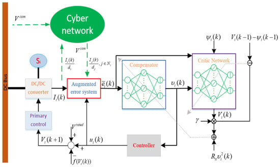
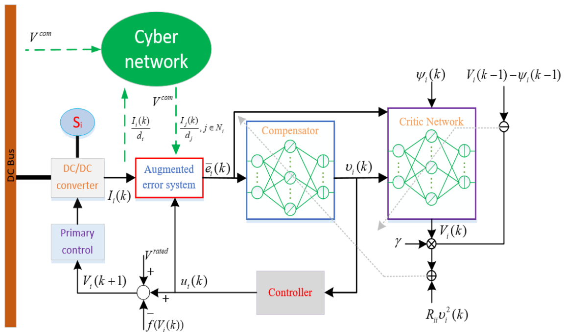
This part details the practical implementation of the SIPI framework. As illustrated in Figure 2, the control architecture for source i comprises an actor network and a critic network. The critic network is used to estimate ${\mathcal{Q}}_i^{(d)}$. The actor network is used to construct $u_i^{(d)}$. Both critic and actor network are three-layer feedforward networks.

Figure 2. The iterative learning control structure for the current-sharing problem.

4.1. Critic Network Design

${\mathcal{Q}}_i^{\left(d\right)}$ is estimated by the critic network, which is realized using a three-layer neural network. Denote $m(\sigma )=[m_1(\sigma ),\dots ,m_{N_{c,i}}(\sigma )]$ and $n(\sigma )=[n_1(\sigma ),\dots ,n_{N_{c,i}}(\sigma )]$, where $N_{c,i}$ is the number of hidden nodes. ${\mathcal{Q}}_i^{\left(d\right)}\left(\sigma \right)$ is designed as

$${\mathcal{Q}}_i^d({\chi }_{I,i}(\sigma ),{\chi }_V(\sigma ),u_i^{(d)}(\sigma ),u_{-i}^{(d)}(\sigma ))=W_{c2,i}^{d}m(\sigma ),$$

(29)

$$m_j(\sigma )=\left(1-e^{-n_j(\sigma )}\right)/\left(1+e^{-n_j(\sigma )}\right), j=1,\dots ,N_{c,i},$$

(30)

$$n(\sigma )=W_{c1,i}^d{\mathcal{X}}_{c,i}(\sigma ),$$

(31)

where $V_i^d(\sigma )$ is the critic network’s output at the dth iteration, and ${\mathcal{X}}_{c,i}(\sigma )={[{\chi }_{I,i}(\sigma ),{\chi }_V(\sigma ),u_i(\sigma )]}^T$ is the critic network’s input. $W_{c1,i}^d\in {\Re }^{N_{c,i}\times 3}$ and $W_{c2,i}^d\in {\Re }^{1\times N_{c,i}}$ are the weights of the first layer and the second layer.

Let ${\mathcal{Q}}_i^{d+1}(\sigma )$ and ${\mathcal{Q}}_i^{d+1}(\sigma +1)$ represent ${\mathcal{Q}}_i^{d+1}({\chi }_{I,i}(\sigma ),{\chi }_V(\sigma ),u_i^{(d)}(\sigma ),u_{-i}^{(d)}(\sigma ))$ and ${\mathcal{Q}}_i^{d+1}({\chi }_{I,i}(\sigma +1),{\chi }_V(\sigma +1),u_i^{(d)}(\sigma +1),u_{-i}^{(d)}(\sigma +1))$, respectively. Accordingly, the prediction error is

$${\xi }_c(\sigma )={\mathcal{Q}}_i^{d+1}(\sigma )-[{\psi }_i(\sigma )+\gamma {\mathcal{Q}}_i^d(\sigma +1)].$$

(32)

The new weighted update error is defined as:

$$E_c(\sigma )={\displaystyle \frac{1}{2}}{\xi }_c^2(\sigma ).$$

(33)

The critic weight at iteration $\tau$ is $W_i^{d+1}(\sigma ){|}_{\tau }$, and its update is given by

$$W_{c2,i}^{d+1}{|}_{\tau +1}=W_{c2,i}^{d+1}{|}_{\tau }+\Delta W_{c2,i}^{d+1}{|}_{\tau },$$

(34)

$$\Delta W_{c2,i}^{d+1}{|}_{\tau }=-\beta \left[{\displaystyle \frac{\partial E_c(\sigma )}{\partial {\xi }_c(\sigma )}}{\displaystyle \frac{\partial {\xi }_c(\sigma )}{\partial {\mathcal{Q}}_i^{d+1}(\sigma )}}{\displaystyle \frac{\partial {\mathcal{Q}}_i^{d+1}(\sigma )}{\partial W_{c2,i}^{d+1}}}\right]{|}_{\tau },$$

(35)

where $\beta$ denotes the step length. If $∥W_{c2,i}^{d+1}{|}_{\tau +1} - W_{c2,i}^{d+1}{|}_{\tau }∥<\epsilon$ is satisfied, then the update terminates.

4.2. Actor Network Design

In this subsection, the constrained policy $u_i^{\left(d\right)}\left(\sigma \right)$ is generated by using a three-layer neural network. Denote $p(\sigma )={[p_1(\sigma ),\dots ,p_{N_{a,i}}(\sigma )]}^T\in {\Re }^{N_{a,i}\times 1}$ and $q(\sigma )={[q_1(\sigma ),\dots ,q_{N_{a,i}}(\sigma )]}^T\in {\Re }^{N_{a,i}\times 1}$. $u_i^{\left(d\right)}\left(\sigma \right)$ is designed as:

$$u_i^d(\sigma )={\Theta }_i(s(\sigma )),$$

(36)

$$s(\sigma )=W_{a2,i}^{d}p(\sigma ),$$

(37)

$$p_j(\sigma )=\left(1-e^{-q_j(\sigma )}\right)/\left(1+e^{-q_j(\sigma )}\right), j=1,\dots ,N_{a,i},$$

(38)

$$q(\sigma )=W_{a1,i}^d{\mathcal{X}}_{a,i}(\sigma ),$$

(39)

where $u_i^d(\sigma )$ represents the output at iteration d, and ${\mathcal{X}}_{a,i}(\sigma )={[{\chi }_{I,i}(\sigma ),{\chi }_V(\sigma )]}^T$ represents the input. The neural network parameters for the first and second layers are given by $W_{a1,i}^d\in {\Re }^{N_{a,i}\times 2}$ and $W_{a2,i}^d\in {\Re }^{1\times N_{a,i}}$, respectively. ${\Theta }_i$ is a bounded injective function, which is selected as

$$\begin{array}{c}\hfill {\Theta }_i(s)={\displaystyle \frac{e^{s/{\overline{u}}_i}-e^{-s/{\overline{u}}_i}}{\frac{1}{{\overline{u}}_i}{e}^{s/{\overline{u}}_i}-\frac{1}{{\underline{u}}_i}{e}^{-s/{\overline{u}}_i}}}\end{array}.$$

Its first derivative ${\Theta }_i^{\prime }=\mathrm{d}{\Theta }_i(·)/\mathrm{d}(·)$ is bounded by $\parallel {\Theta }_i^{\prime }\parallel \le {\Theta }_{iM}$, where ${\Theta }_{iM}>0$.

The prediction error is given by

$$\begin{array}{c}\hfill {\xi }_a(\sigma )=\gamma {\mathcal{Q}}_i^{d+1}(\sigma +1)+{\psi }_i({\chi }_{I,i}(\sigma ),{\chi }_V(\sigma ),u_i^{d+1}(\sigma ),u_{-i}^{d+1}(\sigma )).\end{array}$$

(40)

The new weight update error is defined as:

$$E_a(\sigma )={\displaystyle \frac{1}{2}}{\xi }_a^2(\sigma ).$$

(41)

The actor weight is denoted as $W_{a,i}^{d+1}(\sigma ){|}_{\tau }$. Its update is

$$W_{a2,i}^{d+1}{|}_{\tau +1}=W_{a2,i}^{d+1}{|}_{\tau }+\Delta W_{a2,i}^{d+1}{|}_{\tau },$$

(42)

$$\begin{array}{c}\Delta W_{a2,i}^{d+1}{|}_{\tau }=-\beta \times \hfill \\ \left[{\displaystyle \frac{\partial E_a(\sigma )}{\partial {\xi }_a(\sigma )}}{\displaystyle \frac{\partial {\xi }_a(\sigma )}{\partial u_i^{d+1}(\sigma )}}{\displaystyle \frac{\partial u_i^{d+1}(\sigma )}{\partial W_{a2,i}^{d+1}}}+{\displaystyle \frac{\partial E_a(\sigma )}{\partial {\xi }_a(\sigma )}}{\displaystyle \frac{\partial {\xi }_a(\sigma )}{\partial {\mathcal{Q}}_i^{d+1}(\sigma )}}{\displaystyle \frac{\partial {\mathcal{Q}}_i^{d+1}(\sigma )}{\partial W_{a2,i}^{d+1}}}\right]{|}_{\tau },\hfill \end{array}$$

(43)

where $\beta$ denotes the step length. If $∥W_{a2,i}^{d+1}{|}_{\tau +1} - W_{a2,i}^{d+1}{|}_{\tau }∥<\epsilon$, then the update terminates.

Theorem 2.

For $\forall i\in {\Pi }_S$, let $W_{c2,i}^{\ast }$ and $W_{a2,i}^{\ast }$ be the ideal bounded output-layer weights of the critic and actor networks, respectively. The weights are updated according to the gradient-descent rules given in Section 4. If the learning rate β satisfies

$$0<\beta <min\left\{{\displaystyle \frac{2}{m_M^2}}, {\displaystyle \frac{2\Vert {\tilde{W}}_{a2,i}^{(\tau )}\Vert }{p_M{\Theta }_{iM}\Vert {\xi }_{a,i}\Vert }}\right\},$$

(44)

where $m_M$, $p_M$, and ${\Theta }_{iM}$ are the upper bounds of $\parallel m_i(\sigma )\parallel$, $\parallel p_i(\sigma )\parallel$, and $|{\Theta }_i^{\prime }(s)|$, respectively, then the weight estimation errors are uniformly ultimately bounded (UUB).

Proof. 

Define the weight estimation errors as

$${\tilde{W}}_{c2,i}^{(\tau )}=W_{c2,i}^{(\tau )}-W_{c2,i}^{\ast }, {\tilde{W}}_{a2,i}^{(\tau )}=W_{a2,i}^{(\tau )}-W_{a2,i}^{\ast }.$$

(45)

Then, the error dynamics are

$${\tilde{W}}_{c2,i}^{(\tau +1)}={\tilde{W}}_{c2,i}^{(\tau )}-\beta {\xi }_{c,i}{m}_i, {\tilde{W}}_{a2,i}^{(\tau +1)}={\tilde{W}}_{a2,i}^{(\tau )}-\beta {\xi }_{a,i}{\Theta }_i^{\prime }{p}_i.$$

(46)

Select the Lyapunov function as

$$L_i=\mathrm{tr}\left\{{\tilde{W}}_{c2,i}^{(\tau )T}{\tilde{W}}_{c2,i}^{(\tau )}\right\}+\mathrm{tr}\left\{{\tilde{W}}_{a2,i}^{(\tau )T}{\tilde{W}}_{a2,i}^{(\tau )}\right\}.$$

(47)

The difference of (47) is

$$\begin{array}{cc}\hfill \Delta L_i& =-2\beta {\xi }_{c,i}{\tilde{W}}_{c2,i}^{(\tau )T}{m}_i+{\beta }^2{\xi }_{c,i}^2\parallel m_i{\parallel }^2-2\beta {\xi }_{a,i}{\Theta }_i^{\prime }{\tilde{W}}_{a2,i}^{(\tau )T}{p}_i+{\beta }^2{\xi }_{a,i}^2{({\Theta }_i^{\prime })}^2{\parallel p_i\parallel }^2\hfill \\ \hfill & \le -\beta (2-\beta m_M^2)\Vert {\xi }_{c,i}{\Vert }^2+\beta {\Theta }_{iM}{p}_M\Vert {\xi }_{a,i}\Vert (-2\Vert {\tilde{W}}_{a2,i}^{(\tau )}\Vert +\beta p_M{\Theta }_{iM}\Vert {\xi }_{a,i}\Vert ).\hfill \end{array}$$

(48)

Under condition (44), one has $\Delta L_i<0$. Therefore, the weight estimation errors are UUB. □

Theorem 3.

Suppose that the conditions in Theorems 1 and 2 hold, and that the control law is implemented by the converged actor network, i.e., ${\widehat{u}}_i(\sigma )={\Theta }_i({\widehat{W}}_{a2,i}p(\sigma ))$ for all $i\in {\Pi }_S$. Then there exists a positive constant ${\overline{\epsilon }}_u$ such that $\parallel \widehat{u}(\sigma )-u^{\ast }(\sigma )\parallel \le {\overline{\epsilon }}_u$ for all σ, and the error systems (10) and (11) driven by the approximate policy $\widehat{u}(\sigma )$ are UUB, and $\widehat{u}(\sigma )$ approaches the Nash equilibrium as ${\overline{\epsilon }}_u\to 0$.

Proof. 

By the universal approximation property of neural networks, the optimal policy can be represented as $u_i^{\ast }(\sigma )={\Theta }_i(W_{a2,i}^{\ast }p(\sigma ))+{\epsilon }_{a,i}(\sigma )$, where ${\epsilon }_{a,i}(\sigma )$ is the reconstruction error with $\parallel {\epsilon }_{a,i}(\sigma )\parallel \le {\overline{\epsilon }}_a$ on the compact set $\Omega$. From Theorem 2, the weight estimation errors are UUB, i.e., there exists a constant $b_W>0$ such that $\parallel {\tilde{W}}_{a2,i}\parallel \le b_W$ after convergence. Since ${\Theta }_i$ is Lipschitz with $\parallel {\Theta }_i^{\prime }\parallel \le {\Theta }_{iM}$ and $\parallel p(\sigma )\parallel \le p_M$, by the mean value theorem, one has

$$\parallel {\widehat{u}}_i(\sigma )-u_i^{\ast }(\sigma )\parallel \le {\Theta }_{iM}{p}_M{b}_W+{\overline{\epsilon }}_a\triangleq {\overline{\epsilon }}_u, \forall i\in {\Pi }_S.$$

(49)

Note that the saturating activation ${\Theta }_i$ guarantees that ${\widehat{u}}_i(\sigma )$ always respects the input constraint (5), and hence $\widehat{u}(\sigma )$ is bounded for all $\sigma$ even before convergence.

Since the error dynamics (10) and (11) are linear in the control input, letting $E(\sigma )={[{\chi }_V(\sigma ),{\chi }_{I,1}(\sigma ),\dots ,{\chi }_{I,M}(\sigma )]}^T$ and $u(\sigma )={[u_1(\sigma ),\dots ,u_M(\sigma )]}^T$, the closed-loop system under the approximate joint policy $\widehat{u}(\sigma )$ can be written as

$$E(\sigma +1)=E(\sigma )+h\mathcal{B}{u}^{\ast }(\sigma )+h\mathcal{B}\tilde{u}(\sigma )\triangleq F(E(\sigma ))+\delta (\sigma ),$$

(50)

where $\mathcal{B}$ is the constant input matrix determined by (10) and (11), $\tilde{u}(\sigma )=\widehat{u}(\sigma )-u^{\ast }(\sigma )$ with $\parallel \tilde{u}(\sigma )\parallel \le \sqrt{M}{\overline{\epsilon }}_u$, and $\parallel \delta (\sigma )\parallel \le h\parallel \mathcal{B}\parallel \sqrt{M}{\overline{\epsilon }}_u\triangleq \overline{\delta }$.

From Lemma 1, the origin of the nominal system $E(\sigma +1)=F(E(\sigma ))$ is asymptotically stable, and F is continuous with $F(0)=0$. By the converse Lyapunov theorem, there exists a Lyapunov function $V(E)$ and positive constants $c_1,c_2,c_3,c_4,c_5$ such that $c_1{\parallel E\parallel }^2\le V(E)\le c_2{\parallel E\parallel }^2$, $V(F(E))-V(E)\le -c_3{\parallel E\parallel }^2$, and $|V(E+\delta )-V(E)|\le c_4\parallel E\parallel \parallel \delta \parallel +c_5{\parallel \delta \parallel }^2$. Therefore,

$$\begin{array}{cc}\hfill \Delta V(E(\sigma ))& =V(F(E(\sigma ))+\delta (\sigma ))-V(E(\sigma ))\hfill \\ \hfill & \le -c_3{\parallel E(\sigma )\parallel }^2+c_4\overline{\delta }\parallel E(\sigma )\parallel +c_5{\overline{\delta }}^2,\hfill \end{array}$$

(51)

which is negative whenever

$$\parallel E(\sigma )\parallel >{\displaystyle \frac{c_4\overline{\delta }+\sqrt{c_4^2{\overline{\delta }}^2+4c_3{c}_5{\overline{\delta }}^2}}{2c_3}}\triangleq b_E.$$

(52)

Hence, the tracking errors ${\chi }_V(\sigma )$ and ${\chi }_{I,i}(\sigma )$ under the approximate actor policy are UUB, and the ultimate bound $b_E$ decreases as the NN approximation error ${\overline{\epsilon }}_u$ decreases. Moreover, (61) implies that ${\widehat{u}}_i(\sigma )$ approaches $u_i^{\ast }(\sigma )$ as ${\overline{\epsilon }}_u\to 0$. Since the optimal joint policy ${\{u_i^{\ast }\}}_{i\in {\Pi }_S}$ constitutes the Nash equilibrium by Lemma 1, the implemented policy approaches the Nash equilibrium in the sense of Definition 2 as ${\overline{\epsilon }}_u\to 0$. This completes the proof. □

5. Simulation

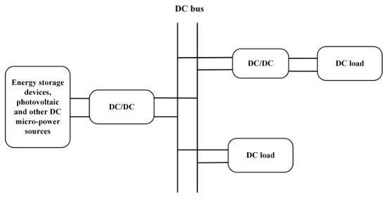
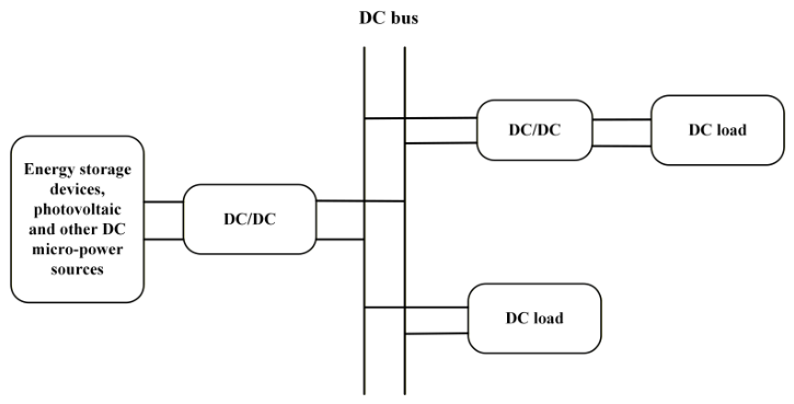
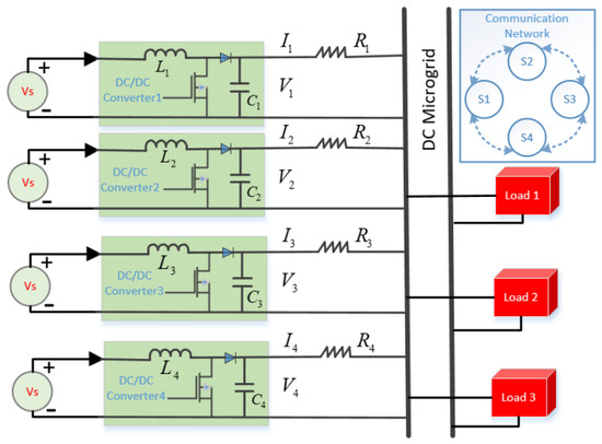
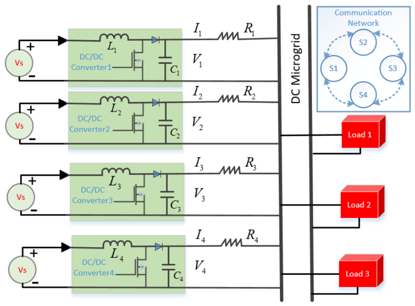
A simulation experiment is conducted to verify the effectiveness of the proposed method. The general DC microgrid diagram consists of a distributed power supply, converter, transmission line, load, etc., as shown in Figure 3. The common distributed DC power supply includes batteries, ultracapacitors, and other energy storage units, and the loads include bulbs, chargers, and other common appliances. The test system shown in Figure 4 is a low-voltage DC microgrid with four parallel-connected sources and three loads, where every source feeds the common bus through a boost-type DC/DC converter. The rated bus voltage is 48 V, the line resistances are set as $R_1=0.2 \Omega$, $R_2=0.3 \Omega$, $R_3=0.25 \Omega$, and $R_4=0.35 \Omega$, and the load resistances are $R_{L1}=20 \Omega$, $R_{L2}=40 \Omega$, and $R_{L3}=40 \Omega$. The DC source voltage is $V_s=12 \mathrm{V}$. The converter inductances are uniform, with $L_1=L_2=L_3=L_4=200 \mu \mathrm{H}$, and the capacitances are $C_1=C_2=C_3=C_4=1000 \mu \mathrm{F}$. $\gamma$ is chosen as $0.95$.

Figure 3. General DC microgrid diagram.

Figure 4. A tested DC microgrid with four power sources and three loads.

Both the actor and critic networks contain five hidden neurons. The structure of the activation function is selected as ${\displaystyle \frac{1-{\exp }^{-(·)}}{1+{\exp }^{-(·)}}}$. The weights of all networks are randomly initialized within the interval $[-1,1]$. To mitigate parameter drift, a projection mechanism with a unit upper bound is adopted; whenever a weight surpasses this limit, it is normalized according to $W_{ji}={\displaystyle \frac{W_{ji}}{\max \left\{W_{ji}\right\}}}$. By dividing by a maximum input, the input of the network is normalized. Specifically, for the actor network, we normalize the input as ${\displaystyle \frac{{\mathcal{X}}_{a,i}}{E}}$, where E is set to 4. For the critic network, we normalize the input as $\left\{{\chi }_{I,i},{\chi }_V,u_i\right\}$. In the simulation test, we set ${\overline{u}}_i=0.2$ and ${\underline{u}}_i=-0.1$ for $\forall i=1,2,3,4$. The sharing ratios are set to $(d_1,d_2,d_3,d_4)=(3.5,3,2.5,1)$. The learning rate is set to $\beta =0.05$, and the convergence threshold is $\epsilon ={10}^{-6}$. The maximum iteration is set to 30.

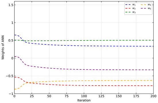
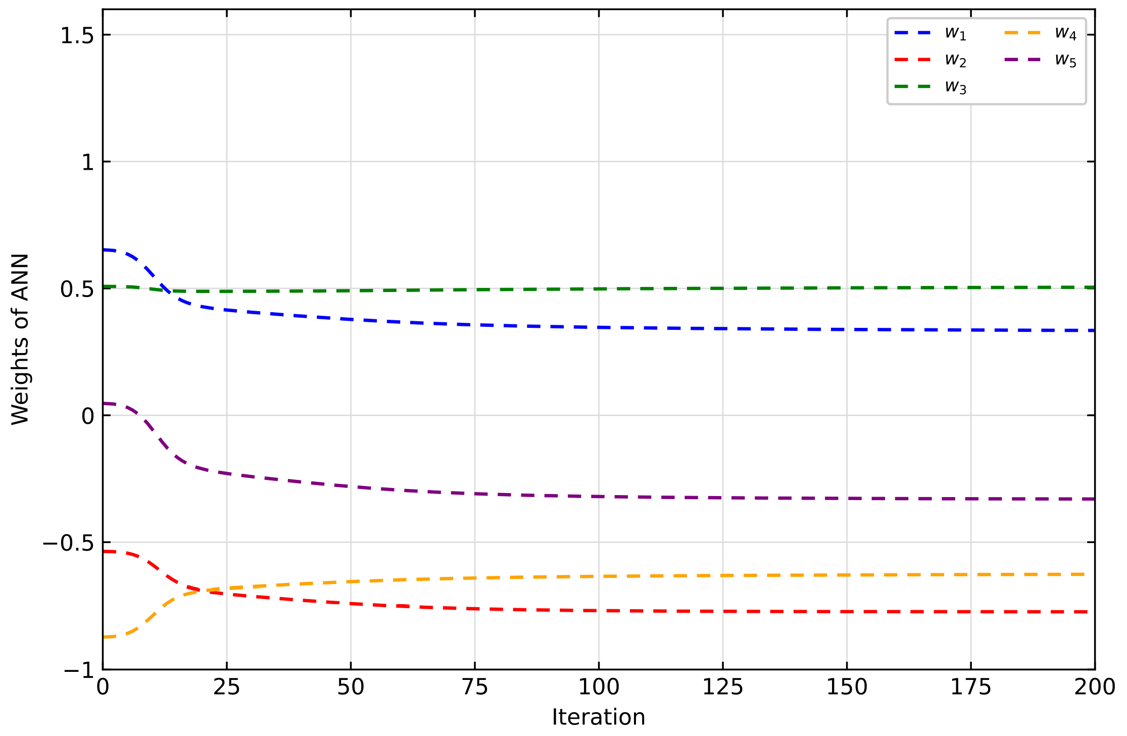
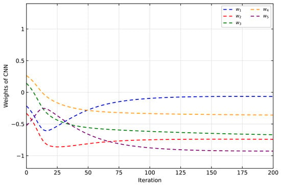
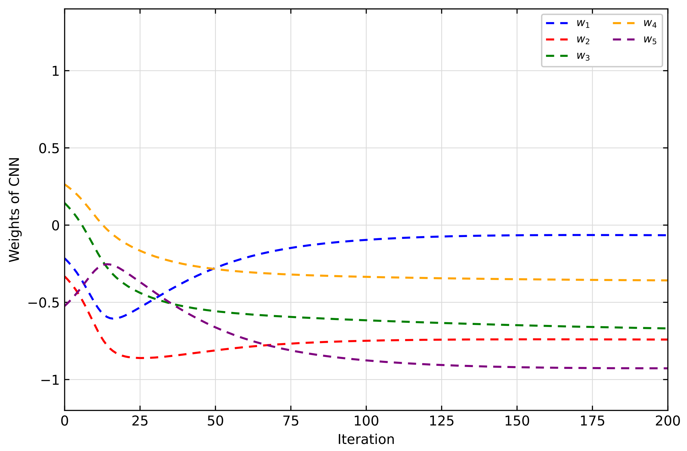
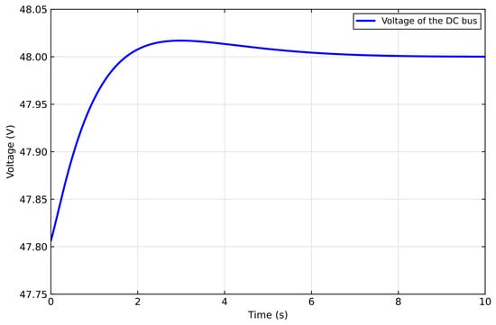
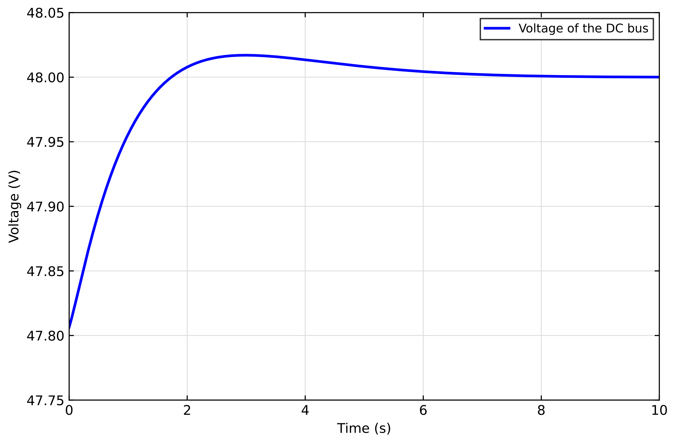
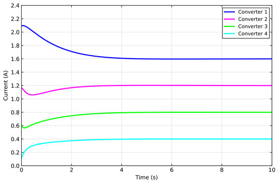
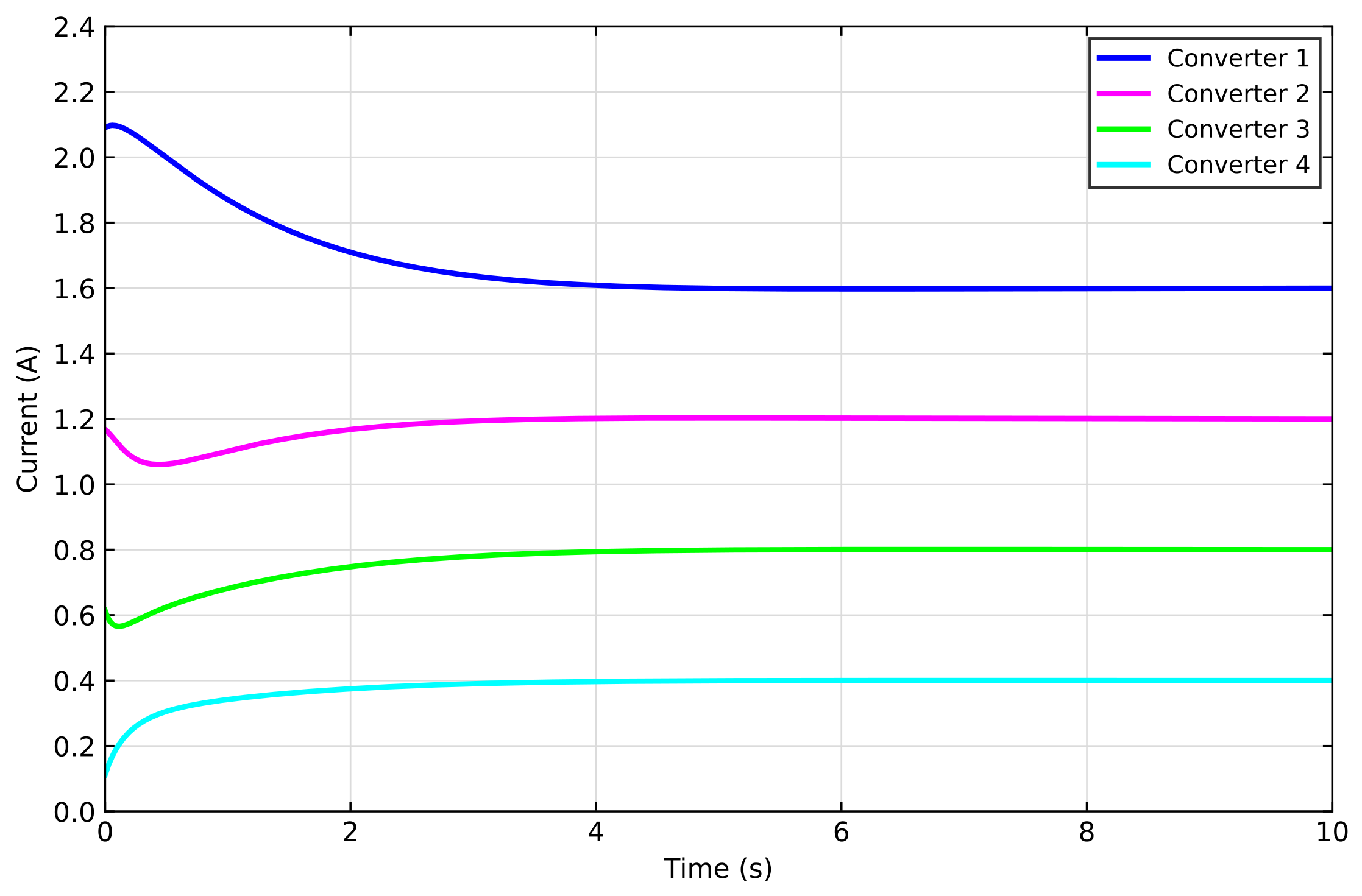
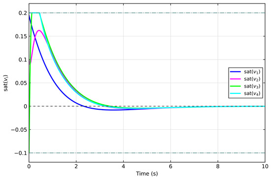
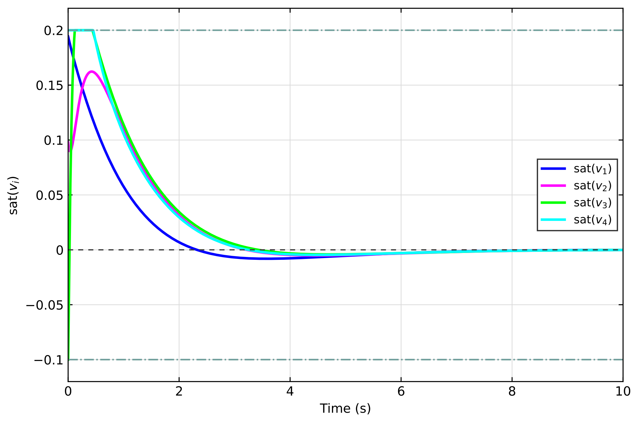
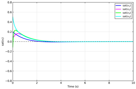
The simulation results are presented in Figure 5, Figure 6, Figure 7, Figure 8 and Figure 9. For source 1, the evolution of $W_{a2,1}$ and $W_{c2,1}$ is depicted in Figure 5 and Figure 6. Figure 7 and Figure 8 show the voltage evolution of the DC bus and the output current evolution of four converters. Figure 9 shows the control input. It can be seen that once the controller input hits its maximum allowable value of $0.2$, it remains clamped at $0.2$. From Figure 5, Figure 6, Figure 7, Figure 8 and Figure 9, the control framework works well.

Figure 5. The weight $W_{a2,1}$ of source 1.

Figure 6. The weight $W_{c2,1}$ of source 1.

Figure 7. Voltage of the DC bus.

Figure 8. Output current of four converters.

Figure 9. Evolution of the constrained control inputs.

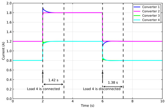
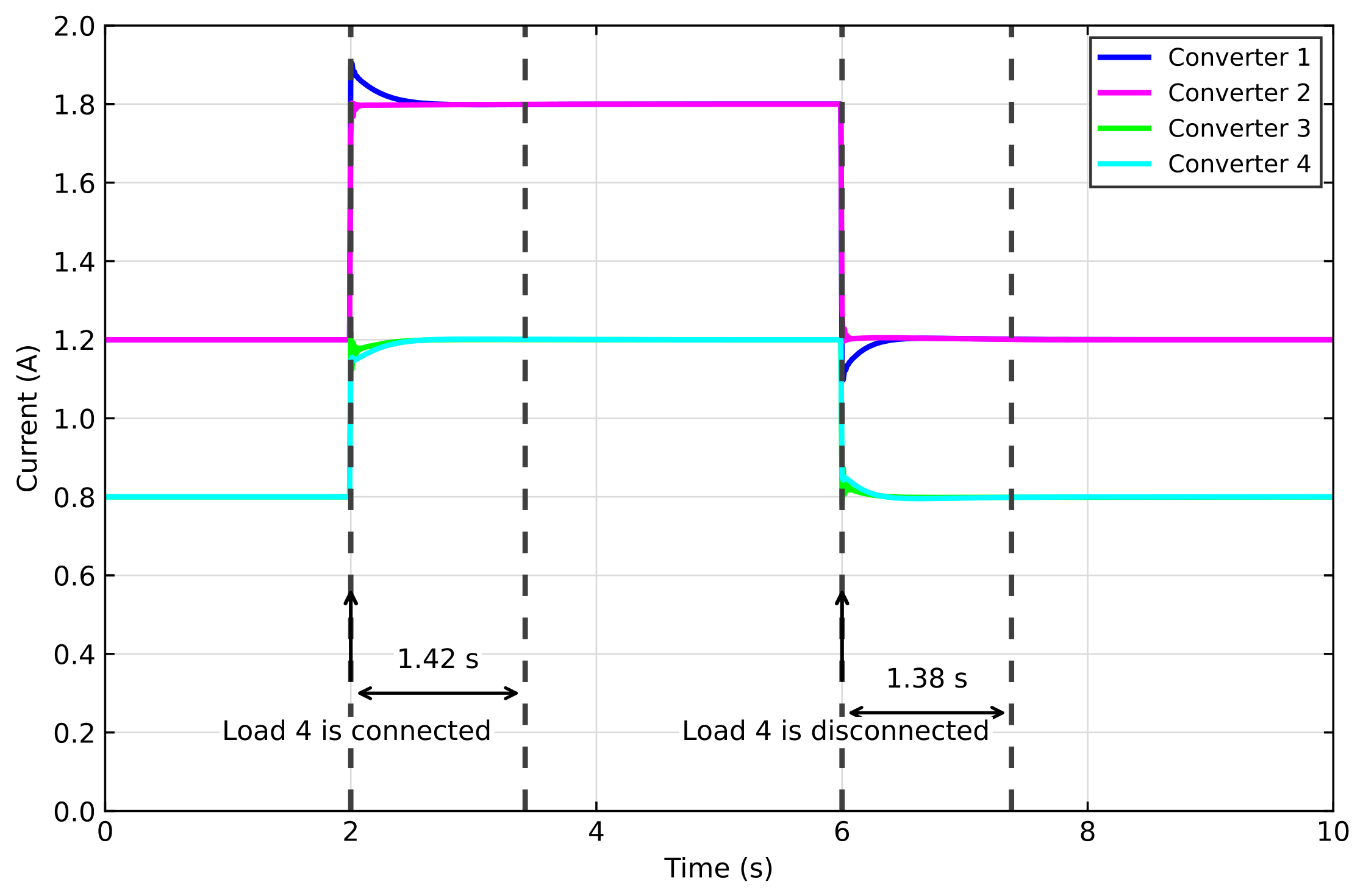
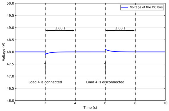
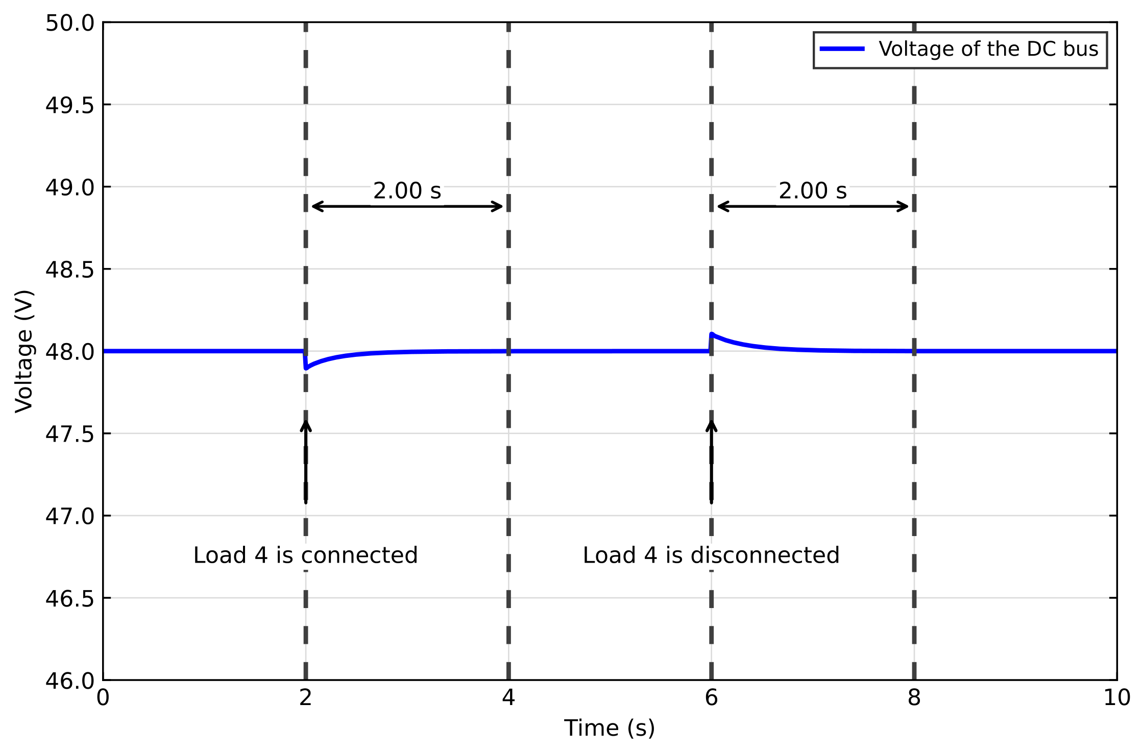
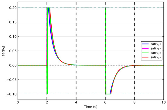
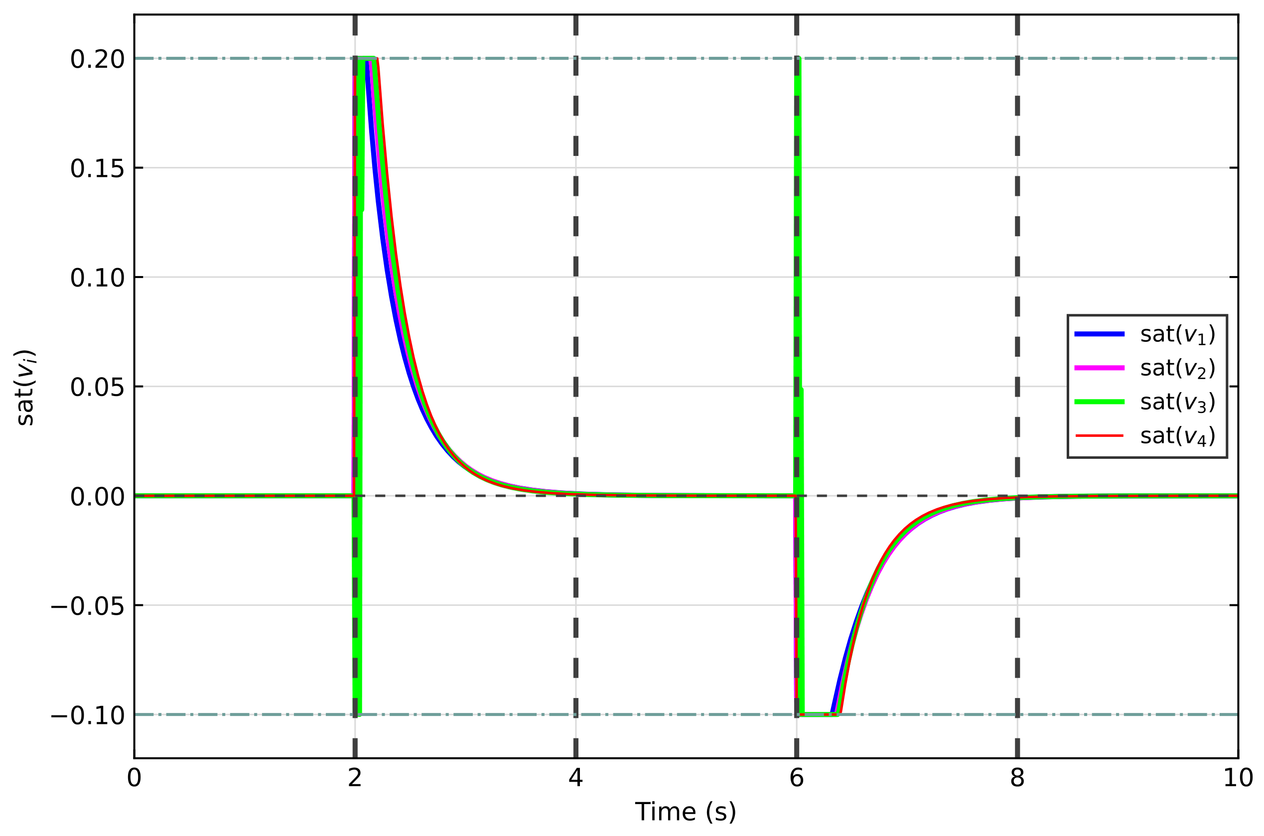
In the following, we test the performance of the SIPI scheme when the load changes. Let $d_1=d_2=0.3$, $d_3=d_4=0.4$. In addition to the aforementioned three loads, a fourth load, Load4 ($20 \Omega$), is introduced to evaluate the controller’s response to load disturbances. We connect the load to the DC bus for a period of time, then disconnect it and observe the voltage, current changes, and control input after the load changes. Figure 10, Figure 11 and Figure 12 depict the dynamic responses of the current and voltage. From Figure 10, Figure 11 and Figure 12, the SIPI scheme maintains satisfactory performance when the network load changes.

Figure 10. The load change test: output current.

Figure 11. The load change test: voltage of the DC bus.

Figure 12. The load change test: control input.

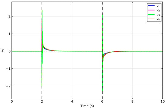
To further demonstrate the necessity of handling input constraints, the proposed SIPI algorithm is compared with the unconstrained RL method in [30]. The control inputs of the unconstrained RL method are shown in Figure 13 and Figure 14. It is clear that the control inputs are unbounded and may exceed the safe system thresholds, which could damage the DC–DC converters and threaten the stability of the microgrid.

Figure 13. Control input of unconstrained RL in [30].

Figure 14. The load change test: control input of unconstrained RL in [30].

6. Conclusions

This article has proposed a novel constrained reinforcement learning architecture to effectively address the challenges of current sharing and voltage regulation in islanded DC microgrids. By utilizing a hyperbolic function, a local cost function incorporating both current and voltage errors was formulated, allowing for the derivation of an optimal control law via the HJB equation. To approximate this optimal policy, a SIPI method was proposed, supported by a rigorous convergence analysis. Furthermore, an actor–critic architecture was constructed to implement this method, employing an asymmetric constrained activation function to specifically handle asymmetric input saturation. Finally, simulation results were presented to verify the effectiveness of the proposed control scheme.

References

- Zhong, X.; Jayawardene, I.; Venayagamoorthy, G.K.; Brooks, R. Denial of service attack on tie-line bias control in a power system with pv plant. IEEE Trans. Emerg. Top. Comput. Intell. 2017, 1, 375–390. [Google Scholar] [CrossRef] [Scilit]
- Ma, W.-J.; Wang, J.; Lu, X.; Gupta, V. Optimal operation mode selection for a DC microgrid. IEEE Trans. Smart Grid 2016, 7, 2624–2632. [Google Scholar] [CrossRef] [Scilit]
- Hamzeh, M.; Ghazanfari, A.; Mohamed, Y.A.-R.I.; Karimi, Y. Modeling and design of an oscillatory current-sharing control strategy in DC microgrids. IEEE Trans. Ind. Electron. 2015, 62, 6647–6657. [Google Scholar] [CrossRef] [Scilit]
- Olivares, D.E.; Mehrizi-Sani, A.; Etemadi, A.H.; Cañizares, C.A.; Iravani, R.; Kazerani, M.; Hajimiragha, A.H.; Gomis-Bellmunt, O.; Saeedifard, M.; Palma-Behnke, R.; et al. Trends in microgrid control. IEEE Trans. Smart Grid 2014, 5, 1905–1919. [Google Scholar] [CrossRef] [Scilit]
- Utkarsh, K.; Trivedi, A.; Srinivasan, D.; Reindl, T. A consensus-based distributed computational intelligence technique for real-time optimal control in smart distribution grids. IEEE Trans. Emerg. Top. Comput. Intell. 2016, 1, 51–60. [Google Scholar] [CrossRef] [Scilit]
- Dörfler, F.; Chertkov, M.; Bullo, F. Synchronization in complex oscillator networks and smart grids. Proc. Natl. Acad. Sci. USA 2013, 110, 2005–2010. [Google Scholar] [CrossRef] [Scilit]
- Lu, X.; Wang, J. A game changer: Electrifying remote communities by using isolated microgrids. IEEE Electrif. Mag. 2017, 5, 56–63. [Google Scholar] [CrossRef] [Scilit]
- Farhangi, H. The path of the smart grid. IEEE Power Energy Mag. 2009, 8, 18–28. [Google Scholar] [CrossRef] [Scilit]
- Kakigano, H.; Miura, Y.; Ise, T.; Uchida, R. DC voltage control of the DC micro-grid for super high quality distribution. In Proceedings of the 2007 Power Conversion Conference-Nagoya, Nagoya, Japan, 2–5 April 2007; IEEE: Piscataway, NJ, USA, 2007; pp. 518–525. [Google Scholar]
- Papadimitriou, C.N.; Zountouridou, E.I.; Hatziargyriou, N.D. Review of hierarchical control in DC microgrids. Electr. Power Syst. Res. 2015, 122, 159–167. [Google Scholar] [CrossRef] [Scilit]
- Bidram, A.; Davoudi, A. Hierarchical structure of microgrids control system. IEEE Trans. Smart Grid 2012, 3, 1963–1976. [Google Scholar] [CrossRef] [Scilit]
- Guerrero, J.M.; Vasquez, J.C.; Matas, J.; De Vicuña, L.G.; Castilla, M. Hierarchical control of droop-controlled AC and DC microgrids—A general approach toward standardization. IEEE Trans. Ind. Electron. 2010, 58, 158–172. [Google Scholar] [CrossRef] [Scilit]
- Yang, L.; Chen, Y.; Luo, A.; Wu, W.; Huai, K.; Zhou, X.; Zhou, L.; Xu, Q.; Guerrero, J.M. Second ripple current suppression by two bandpass filters and current sharing method for energy storage converters in DC microgrid. IEEE J. Emerg. Sel. Top. Power Electron. 2016, 5, 1031–1044. [Google Scholar] [CrossRef] [Scilit]
- Yang, J.; Jin, X.; Wu, X.; Acuna, P.; Aguilera, R.P.; Morstyn, T.; Agelidis, V.G. Decentralised control method for DC microgrids with improved current sharing accuracy. IET Gener. Transm. Distrib. 2017, 11, 696–706. [Google Scholar] [CrossRef] [Scilit]
- Augustine, S.; Mishra, M.K.; Lakshminarasamma, N. Adaptive droop control strategy for load sharing and circulating current minimization in low-voltage standalone DC microgrid. IEEE Trans. Sustain. Energy 2014, 6, 132–141. [Google Scholar] [CrossRef] [Scilit]
- Wang, P.; Lu, X.; Yang, X.; Wang, W.; Xu, D. An improved distributed secondary control method for DC microgrids with enhanced dynamic current sharing performance. IEEE Trans. Power Electron. 2015, 31, 6658–6673. [Google Scholar] [CrossRef] [Scilit]
- Lu, X.; Guerrero, J.M.; Sun, K.; Vasquez, J.C. An improved droop control method for dc microgrids based on low bandwidth communication with dc bus voltage restoration and enhanced current sharing accuracy. IEEE Trans. Power Electron. 2013, 29, 1800–1812. [Google Scholar] [CrossRef] [Scilit]
- Anand, S.; Fernandes, B.G.; Guerrero, J. Distributed control to ensure proportional load sharing and improve voltage regulation in low-voltage DC microgrids. IEEE Trans. Power Electron. 2012, 28, 1900–1913. [Google Scholar] [CrossRef] [Scilit]
- Guo, F.; Xu, Q.; Wen, C.; Wang, L.; Wang, P. Distributed secondary control for power allocation and voltage restoration in islanded DC microgrids. IEEE Trans. Sustain. Energy 2018, 9, 1857–1869. [Google Scholar] [CrossRef] [Scilit]
- Yang, Q.; Jiang, L.; Zhao, H.; Zeng, H. Autonomous voltage regulation and current sharing in islanded multi-inverter DC microgrid. IEEE Trans. Smart Grid 2017, 9, 6429–6437. [Google Scholar] [CrossRef] [Scilit]
- Sahoo, S.; Mishra, S. A distributed finite-time secondary average voltage regulation and current sharing controller for DC microgrids. IEEE Trans. Smart Grid 2017, 10, 282–292. [Google Scholar] [CrossRef] [Scilit]
- Nasirian, V.; Moayedi, S.; Davoudi, A.; Lewis, F.L. Distributed cooperative control of DC microgrids. IEEE Trans. Power Electron. 2014, 30, 2288–2303. [Google Scholar] [CrossRef] [Scilit]
- Xiang, J.; Wang, Y.; Li, Y.; Wei, W. Stability and steady-state analysis of distributed cooperative droop controlled DC microgrids. IET Control Theory Appl. 2016, 10, 2490–2496. [Google Scholar] [CrossRef] [Scilit]
- Lu, X.; Sun, K.; Guerrero, J.M.; Vasquez, J.C.; Huang, L. State-of-charge balance using adaptive droop control for distributed energy storage systems in DC microgrid applications. IEEE Trans. Ind. Electron. 2013, 61, 2804–2815. [Google Scholar] [CrossRef] [Scilit]
- Shen, Z.; Dong, T. Event-Based Receding-Horizon Q-Learning Control of Nonlinear Discrete-Time Systems with Asymmetric Control Constraints. IEEE Trans. Emerg. Top. Comput. Intell. 2026. [Google Scholar] [CrossRef] [Scilit]
- Sun, S.; Endo, T.; Matsuno, F. Iterative learning control based robust distributed algorithm for non-holonomic mobile robots formation. IEEE Access 2018, 6, 61904–61917. [Google Scholar] [CrossRef] [Scilit]
- Norrlof, M.; Gunnarsson, S. Experimental comparison of some classical iterative learning control algorithms. IEEE Trans. Robot. Autom. 2002, 18, 636–641. [Google Scholar] [CrossRef] [Scilit]
- Dong, T.; Gong, X.; Wang, A.; Li, H.; Huang, T. Data-Driven Tracking Control for Multi-Agent Systems with Unknown Dynamics via Multithreading Iterative Q-Learning. IEEE Trans. Syst. Man Cybern. Syst. 2023, 53, 2533–2542. [Google Scholar] [CrossRef] [Scilit]
- Dong, T.; Li, Y. Prescribed-Time Bipartite Synchronization of Fuzzy Signed Networks via Fuzzy Reinforcement Learning. IEEE Trans. Emerg. Top. Comput. Intell. 2026, 10, 2901–2909. [Google Scholar] [CrossRef] [Scilit]
- Chaturvedi, S.; Bui, V.; Su, W.; Wang, M. Reinforcement Learning-Based Integrated Control to Improve the Efficiency of DC Microgrids. IEEE Trans. Smart Grid 2024, 15, 149–159. [Google Scholar] [CrossRef] [Scilit]
- Zeng, Y.; Pou, J.; Sun, C.; Li, X.; Liang, G.; Xia, Y.; Mukherjee, S.; Gupta, A.K. Deep Reinforcement Learning-Enabled Distributed Uniform Control for a DC Solid State Transformer in DC Microgrid. IEEE Trans. Ind. Electron. 2024, 71, 5818–5829. [Google Scholar] [CrossRef] [Scilit]
- Fan, Z.; Zhang, W.; Liu, W. Multi-Agent Deep Reinforcement Learning-Based Distributed Optimal Generation Control of DC Microgrids. IEEE Trans. Smart Grid 2023, 14, 3337–3351. [Google Scholar] [CrossRef] [Scilit]
- Zhang, X.; Li, P.; Zhang, Y.; Huang, D.; Wang, B.; Zhou, Y.; Huo, F.; Ukil, A. Reinforcement Learning Based Active Model Variation Deadbeat Control for Energy Storage System in DC Microgrids with Constant Power Loads. IEEE Trans. Ind. Electron. 2026, 73, 2427–2439. [Google Scholar] [CrossRef] [Scilit]
- Fan, Z.; Zhang, W.; Liu, W. Data-Efficient Deep Reinforcement Learning-Based Optimal Generation Control in DC Microgrids. IEEE Syst. J. 2024, 18, 426–437. [Google Scholar] [CrossRef] [Scilit]
- Yuan, Z.; Zeng, Y.; Ghias, A.M.Y.M.; Pou, J.; Pickert, V. Online-Trained Deep Reinforcement Learning-Based Control for Reconfigurable Battery Storage in DC Shipboard Microgrid Applications. IEEE Trans. Transp. Electrif. 2026, 12, 3625–3639. [Google Scholar] [CrossRef] [Scilit]
- Abu-Khalaf, M.; Lewis, F.L. Nearly optimal control laws for nonlinear systems with saturating actuators using a neural network HJB approach. Automatica 2005, 41, 779–791. [Google Scholar] [CrossRef] [Scilit]
- Dong, L.; Zhong, X.; Sun, C.; He, H. Event-Triggered Adaptive Dynamic Programming for Continuous-Time Systems with Control Constraints. IEEE Trans. Neural Netw. Learn. Syst. 2017, 28, 1941–1952. [Google Scholar] [CrossRef] [Scilit]
- Dong, T.; Li, K.; Huang, T. Event-Based ADP Tracking Control of Complex-Valued Nonlinear Systems. IEEE Trans. Emerg. Top. Comput. Intell. 2024, 8, 1086–1096. [Google Scholar] [CrossRef] [Scilit]
- Liu, D.; Wei, Q. Policy iteration adaptive dynamic programming algorithm for discrete-time nonlinear systems. IEEE Trans. Neural Netw. Learn. Syst. 2013, 25, 621–634. [Google Scholar] [CrossRef] [Scilit]
- Shen, Z.; Dong, T.; Huang, T. Data-driven bipartite synchronization control of multi-agent systems with asymmetric input saturation over switching networks. Appl. Math. Comput. 2025, 494, 129280. [Google Scholar] [CrossRef] [Scilit]
- Lei, J.; Shanbhag, U.V. Distributed variable sample-size gradient-response and best-response schemes for stochastic Nash equilibrium problems. SIAM J. Optim. 2022, 32, 573–603. [Google Scholar] [CrossRef] [Scilit]
Disclaimer/Publisher’s Note: The statements, opinions and data contained in all publications are solely those of the individual author(s) and contributor(s) and not of MDPI and/or the editor(s). MDPI and/or the editor(s) disclaim responsibility for any injury to people or property resulting from any ideas, methods, instructions or products referred to in the content. |
© 2026 by the authors. Licensee MDPI, Basel, Switzerland. This article is an open access article distributed under the terms and conditions of the Creative Commons Attribution (CC BY) license.