Exact Solutions of Higher-Dimensional Integrable Models Using Extended Trial Functions Within a Symbolic Neural Network Computation

Abstract

This paper investigates two integrable $(2+1)$-dimensional nonlinear evolution equations, namely the Kairat–II–X-extended (K–II–X-E) model and the Kairat–II-X (K–II–X)-type model, with the objective of deriving exact analytical soliton solutions. These models serve as fundamental prototypes for nonlinear wave dynamics and arise in a broad range of physical contexts, including fluid flows, optical signal propagation, plasma media, and selected biological systems. A $(G^{\prime }/G)$-expansion neural networks (ENNs) framework is developed by rigorously coupling the algebraic mechanism of the classical method with the symbolic neural networks. This unified strategy enables the systematic construction of exact analytical solutions directly from the governing equations. Using this framework, exact one- and two-soliton solutions are constructed, along with a broader class of nonlinear wave structures, demonstrating the capability of the method to capture diverse solution dynamics. The resulting solutions are expressed explicitly in trigonometric, hyperbolic, and rational forms. The dynamical features of the obtained solutions are further illustrated through 2D and 3D surface and polar plots, which reveal their localization properties, propagation characteristics, and interaction patterns in higher-dimensional settings. The results show that the $(G^{\prime }/G)$-ENNs method provides an efficient and systematic framework for constructing exact solutions of nonlinear evolution equations. This approach offers a promising analytical tool for investigating complex wave phenomena and underscores the potential of neural-network-assisted symbolic techniques in advancing research in nonlinear mathematical physics.

1. Introduction

Nonlinear partial differential equations (NPDEs) are used in a fundamental mathematical model that is used to model multifaceted wave phenomena in a wide range of science and engineering fields. Their important role can be seen in the models of optical soliton propagation and modulation instability in optical fibers [1] and dynamics of waves in harbors and coastal areas [2,3] and waves in shallow water [4]. NPDEs contain, equally, the description of reaction–diffusion processes [5], matter–wave dynamics in Bose–Einstein condensates [6], the evolution of biological populations [7], and many other engineering systems [8]. In all of these fields, the identification and study of coherent structures, such as solitons, lump waves, and breathers, is required for further theoretical developments and practical applications. Construction of accurate solutions to NPDEs is the province of applied mathematics and has been informed by the need to understand complex natural systems at a high fidelity level. Historically, this pursuit has been based on special analytical methods that are aimed at finding exact, interpretable solutions for basic models. However, these classical methods often face a major hurdle, which is that the algebra operations become hugely difficult for the modern-day equations, which are highly dimensional, and may be impossible in many cases. In response, a complimentary paradigm has emerged based on sophisticated computational frameworks. These frameworks are implemented not simply as a replacement for analytical work but to transform. Their purpose is to short-cut the bottlenecks that are present in purely analytic approaches to make it easier to find compact sets of solutions that are out of reach of conventional symbolic analysis.

The great significance of NPDEs is offset by the great difficulty associated with their analysis. The nonlinear mechanisms they encode often have sensitive dynamics and are often dictated by chaotic dynamics where the results are acutely dependent on initial conditions as well as parameters so that long-term prediction and control is inherently difficult [9]. A wide variety of sophisticated approaches in analyzing properties of nonlinear models and exact soliton-type solutions of NPDEs have been developed. Notable techniques include the $(G^{\prime }/G)$-expansion method [10,11], the ${\varphi }^6$-model expansion method [12], the Kudryashov method [13], the modified auxiliary equation technique [14], the modified exponential rational function method [15], the generalized Riccati mapping method [16], the improved F-expansion method [17], the Khater II method [18], the Sardar sub-equation approach [19], the auto-Bäcklund transformation approach [20], the Jacobi elliptic function expansion technique [21], the sine–cosine methods [22], the Kumar–Malik method [23], the $(G^{\prime }/G,1/G)$-expansion method [24], extended Jacobi elliptic expansions [25], the inverse scattering transform [26], the improved modified extended tanh method [27], and the Hirota bilinear method [28]. More recently, the integration of direct analytical methods with symbolic neural network architectures has led to the development of Hirota bilinear neural networks (BNNs) [29]. This synergy promises to provide bridging ground value, as well as a modern computational framework coupled with classical analytical techniques, to help obtain multi-soliton solutions in systematic construction and analyze the dynamics of interactions of a complex nature. Nevertheless, these results highlight a long-standing challenge in the field: finding a generalized analytical method for the solution of all classes of NPDEs is a goal still to be achieved.

In recent years, artificial intelligence and deep learning, in particular, have become powerful tools in a wide range of scientific and technological domains [30,31]. Neural networks (NNs), with their universal approximation property and strong representational capability, have played a central role in recent developments [32]. They have achieved remarkable success in areas such as image classification [33], computer vision [34], and natural language processing [35]. Sekban et al. [36] investigated the formability behavior of high-strength shipbuilding steel using experimental analysis, finite element modeling, and artificial NNs. Liu et al. [37] proposed a $(G^{\prime }/G)$-ENN method to obtain exact explicit solutions of NPDEs, providing an effective framework for constructing diverse wave solutions. More recently, deep learning techniques have been extended to the study of PDEs, where NNs are employed as trial function representations of solution spaces, enabling the treatment of complex and challenging mathematical models and contributing significantly to the field of scientific machine learning [38]. Beyond PDEs, NNs have also been widely applied to differential and integral equations due to their strong function approximation capability [39,40], with rapid progress demonstrating their effectiveness in handling complex mathematical models [41,42]. In this context, physics-informed neural networks (PINNs) [43,44] have emerged as a powerful tool for approximating solutions of differential equations. Tipu et al. [45] combined PINNs with polynomial expansion and $(G^{\prime }/G,1/G)$-expansion methods as a hybrid machine learning framework. However, recent research has increasingly focused on NN–based approaches capable of constructing exact analytical solutions. In this direction, bilinear NN frameworks and symbolic neural methods have shown significant progress in solving nonlinear evolution equations, revealing rich wave phenomena such as solitons, lumps, and breather interactions. For instance, localized wave solutions have been reported using Darboux transformation–based LPNN methods [46], bilinear neural architectures for lump–breather dynamics [47], and hybrid neural symbolic approaches for higher-dimensional systems [48]. These studies highlight the growing effectiveness of NN–inspired analytical techniques in nonlinear science. Along these lines, Mateen et al. [49] introduced a NN–based analytical approach that constructs trial functions yielding exact solutions without numerical error. This idea was further developed by Isah et al. [50], who systematically applied the bilinear NN method to nonlinear evolution equations and analyzed the influence of network architecture on solution behavior.

Several analytical techniques have been employed in recent years to derive traveling wave solutions of the K-II-X-E and K-II-X type equations. The K-II type equation has been studied in different forms in recent years. Wu et al. considered nonlinear K-II-X-type models and discussed complex and mixed hyperbolic properties, obtaining several complex wave solutions [51]. Faridi et al. used Lie point symmetries and the Painlevé analysis to derive exact solutions and to examine integrability [52]. Awadalla et al. applied three analytical methods to the M-fractional K-II and K-X type equations and obtained soliton solutions [53]. Demirbilek et al. studied the combined K-II-X type system and reported analytical solutions together with bifurcation, chaotic behavior, energy distribution, and sensitivity analysis [54]. Wazwaz investigated the $(3+1)$-dimensional K-II and K-X type equations and derived multi-soliton, lump, and breather-type solutions, as well as Painlevé results [55]. Mehanna and Wazwaz proposed a tri-analytical method for obtaining exact solutions of the K-II and K-II-X type equations [56]. Mateen et al. used the Kumar–Malik method and the extended hyperbolic function method to construct soliton and traveling wave solutions [57]. Alhakim et al. analyzed bifurcation behavior, chaos, and soliton dynamics using two analytical schemes [58]. Awadalla et al. also presented M-fractional analytical solutions for the K-II and K-X type equations [59]. These works cover soliton solutions, integrability, fractional formulations, bifurcation behavior, and analytical methods for the K-II type equation. While powerful analytical techniques have successfully revealed rich families of multiple soliton and lump wave solutions for these systems [60], the exploration of their full dynamical landscape, particularly for complex, non-analytical initial conditions or parameter regimes, remains a challenge.

Motivated by the intricate nonlinear dynamics of the underlying models, this work uncovers previously unexplored classes of solitary wave solutions for the K-II-X-extended and K-II-X-type equations through a newly developed hybrid $\left(G^{\prime }/G\right)$-ENNs framework. The proposed methodology integrates the analytical strength of the $\left(G^{\prime }/G\right)$-expansion technique with enhanced NNs, forming a unified structure capable of capturing complex nonlinear wave behaviors beyond the reach of existing approaches. To the best of our knowledge, this hybrid $(G^{\prime }/G)$-ENNs based strategy is introduced for the first time for these equations. Furthermore, a novel activation function is designed and systematically analyzed which is the first application in the NN assisted analytical investigations of Kairat-type equations.

In order to resolve NPDEs in the current study, the applications of a recently introduced hybrid methodology with the $\left(G^{\prime }/G\right)$-expansion strategy incorporated within a NN architecture were focused. Four major advancements are realized by this $\left(G^{\prime }/G\right)$-ENNs method:

• A novel activation function using the formulation of $\left(G^{\prime }/G\right)$ is incorporated into the customized neural network framework with analytical trial solutions of the NPDEs being built directly by feedforward operations.
• The proposed method makes no use of pre-existing or training datasets, and therefore results in a huge reduction of the computational cost.
• The resulting solutions are fully analytical and do not contain numerical discretization errors while also identifying new families of solutions instead of just reproducing known solutions.
• The framework provides a clear and systematic approach for building trial solutions and is highly flexible, so that it can easily be extended to various classes of NPDEs by appropriate modifications of the functional structure.

This methodology offers a versatile and efficient methodology to deal with a wide range of NPDEs and establishes a common and innovative methodology for analytical solution construction.

The K-II-X-E- and K-II-X-type equations are generally used to model the nonlinear dynamics of waves in the case of fluid motion, optical communication systems, plasma interaction, and the quantum mechanical processes. Analytical investigation of these models is very important for the understanding of nonlinear dispersive behavior, wave breaking, chaotic patterns, energy transfer mechanism, etc. Obtaining exact solitary wave solutions gives fundamental insight into wave propagation and stability in complex media. The results presented in this study have potential applications in a number of physical environments where nonlinear wave propagation is predominant. The acquired soliton wave structures can provide contribution to the research of shallow water flows, ion-acoustic plasma waves, and nonlinear optical pulses in fiber channels. The novelty of this research is the application of the $(G^{\prime }/G)$-ENNs method combining NNs and symbolic computation in order to construct exact solutions directly without the need for classical similarity transform and restrictive assumptions of ansatzes. This hybrid approach is successful in generating a wide variety of soliton solution families, including dark, periodic, kink, two-kink, dark-kink, and singular soliton structures in trigonometric, hyperbolic, and rational forms, thereby providing a flexible and efficient framework for describing complex nonlinear wave dynamics with high accuracy and computational effectiveness.

This paper is structured as follows. Section 2 presents the methodology of the proposed $(G^{\prime }/G)$-ENNs method. Section 3 applies the method to derive exact solutions of the K-II-X-E- and K-II-X-type equations. Section 4 discusses the results and provides a detailed graphical analysis of the obtained solutions. Finally, Section 5 concludes this study by summarizing the main findings and highlighting potential applications.

2. Methodology

In this section, the $\left(G^{\prime }/G\right)$-expansion method is presented for deriving analytical solutions to NPDEs. We consider a general NPDE of the form

$$\begin{array}{c}\hfill \mathcal{L}\left\{\mathrm{{\rm Y}}\right(x,y,t\left)\right\}+\chi \left\{\mathrm{{\rm Y}}\right(x,y,t\left)\right\}=0.\end{array}$$

(1)

The function $\mathrm{{\rm Y}}(x,y,t)$ represents the unknown solution to be determined. The operators $\mathcal{L}\left\{\mathrm{{\rm Y}}\right(x,y,t\left)\right\}$ and $\chi \left\{\mathrm{{\rm Y}}\right(x,y,t\left)\right\}$ denote the linear and nonlinear components of the equation, respectively, both acting on $\mathrm{{\rm Y}}(x,y,t)$ and its partial derivatives with respect to x, y, and t.

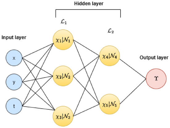
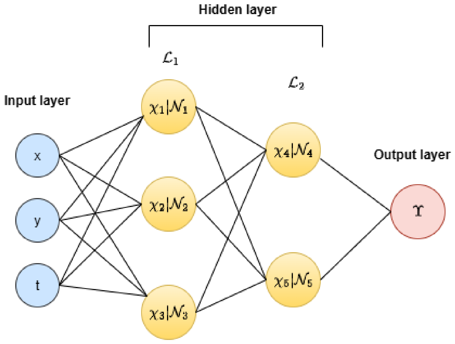
The main idea of the method is to construct a trial solution to approximate $\mathrm{{\rm Y}}(x,y,t)$ using an appropriate analytical form. By substituting this trial function into Equation (1), the PDE is reduced to a system of nonlinear algebraic equations, which are then solved to obtain the network parameters (weights and biases). To achieve this, we design a specific NN architecture consisting of two hidden layers, denoted by ${\mathcal{L}}_1$ and ${\mathcal{L}}_2$, with three and two neurons, as illustrated in Figure 1.

Figure 1. Architecture of NNs.

The mapping corresponding to this network can be expressed as

$$\begin{array}{c}\hfill \left\{\begin{array}{c}{\chi }_1=t w_{t1}+x w_{x1}+y w_{y1},\hfill \\ {\chi }_2=t w_{t2}+x w_{x2}+y w_{y2},\hfill \\ {\chi }_3=t w_{t3}+x w_{x3}+y w_{y3},\hfill \\ {\chi }_4=w_{13}{\mathcal{N}}_1\left({\chi }_1\right)+w_{23}{\mathcal{N}}_2\left({\chi }_2\right)+w_{33}{\mathcal{N}}_3\left({\chi }_3\right),\hfill \\ {\chi }_5=w_{14}{\mathcal{N}}_1\left({\chi }_1\right)+w_{24}{\mathcal{N}}_2\left({\chi }_2\right)+w_{34}{\mathcal{N}}_3\left({\chi }_3\right),\hfill \\ \mathrm{{\rm Y}}(x,y,t)=w_{3\mathrm{{\rm Y}}}{\mathcal{N}}_4\left({\chi }_4\right)+w_{4\mathrm{{\rm Y}}}{\mathcal{N}}_5\left({\chi }_5\right)+b.\hfill \end{array}\right.\end{array}$$

(2)

In this network, the first hidden layer’s initial neurons produce outputs ${\chi }_1$, ${\chi }_2$, and ${\chi }_3$, while ${\chi }_4$ and ${\chi }_5$ are the outputs from the first three neurons in the second hidden layer. Each neuron utilizes its own activation function (${\mathcal{N}}_1$, ${\mathcal{N}}_2$, ${\mathcal{N}}_3$, ${\mathcal{N}}_4$, and ${\mathcal{N}}_5$). The connections between these neurons are characterized by the weights ($w_{t1},w_{t2},w_{t3},w_{x1},w_{x2},w_{x3},w_{y1},w_{y2},w_{y3},w_{13},w_{23},w_{33},w_{14},w_{24},w_{34},w_{3\mathrm{{\rm Y}}},w_{4\mathrm{{\rm Y}}}$), and the biases b and $b_1$ are incorporated to adjust the neuron outputs. The trial function $\mathrm{{\rm Y}}(x,y,t)$ for Equation (1) is explicitly constructed from this complete set of trainable parameters within the network.

In the framework of the proposed scheme, the activation functions ${\mathcal{N}}_1$, ${\mathcal{N}}_2$, and ${\mathcal{N}}_3$ in the first hidden layer are chosen to be a special function $\psi (·)$, defined as

$$\psi \left({\chi }_i\right)=\left(G^{\prime }/G\right)=\left\{\begin{array}{cc}-{\displaystyle \frac{\breve{\lambda }}{2}}+{\displaystyle \frac{\sqrt{{\breve{\lambda }}^2-4\breve{\kappa }}}{2}} {\displaystyle \frac{{\breve{\mathcal{S}}}_1\sinh \left(\frac{1}{2}\sqrt{{\breve{\lambda }}^2-4\breve{\kappa }} {\chi }_i\right)+{\breve{\mathcal{S}}}_2\cosh \left(\frac{1}{2}\sqrt{{\breve{\lambda }}^2-4\breve{\kappa }} {\chi }_i\right)}{{\breve{\mathcal{S}}}_1\cosh \left(\frac{1}{2}\sqrt{{\breve{\lambda }}^2-4\breve{\kappa }} {\chi }_i\right)+{\breve{\mathcal{S}}}_2\sinh \left(\frac{1}{2}\sqrt{{\breve{\lambda }}^2-4\breve{\kappa }} {\chi }_i\right)}},\hspace{1em}\hfill & {\breve{\lambda }}^2-4\breve{\kappa }>0,\hfill \\ -{\displaystyle \frac{\breve{\lambda }}{2}}+{\displaystyle \frac{\sqrt{ 4\breve{\kappa }-{\breve{\lambda }}^2 }}{2}} {\displaystyle \frac{-{\breve{\mathcal{S}}}_1\sin \left(\frac{1}{2}\sqrt{ 4\breve{\kappa }-{\breve{\lambda }}^2 } {\chi }_i\right)+{\breve{\mathcal{S}}}_2\cos \left(\frac{1}{2}\sqrt{ 4\breve{\kappa }-{\breve{\lambda }}^2 } {\chi }_i\right)}{{\breve{\mathcal{S}}}_1\cos \left(\frac{1}{2}\sqrt{ 4\breve{\kappa }-{\breve{\lambda }}^2 } {\chi }_i\right)+{\breve{\mathcal{S}}}_2\sin \left(\frac{1}{2}\sqrt{ 4\breve{\kappa }-{\breve{\lambda }}^2 } {\chi }_i\right)}},\hspace{1em}\hfill & {\breve{\lambda }}^2-4\breve{\kappa }<0,\hfill \\ -{\displaystyle \frac{\breve{\lambda }}{2}}+{\displaystyle \frac{{\breve{\mathcal{S}}}_2}{{\breve{\mathcal{S}}}_1+{\breve{\mathcal{S}}}_2{\chi }_i}},\hspace{1em}\hfill & {\breve{\lambda }}^2-4\breve{\kappa }=0,\hfill \end{array}\right.$$

(3)

where $G=G\left(\breve{\varsigma }\right)$ satisfies a second-order linear ODE,

$$\begin{array}{c}\hfill G^{″}+\breve{\lambda }{G}^{\prime }+\breve{\kappa }G=0,\end{array}$$

(4)

where $\breve{\lambda }$ and $\breve{\kappa }$ are constants determined during the solution.

Thus, the solutions of the NPDEs are constructed in the form of finite polynomials in $\left(G^{\prime }/G\right)$. The proposed solution strategy can be formulated as the Algorithm 1:

Algorithm 1 Neural-Network-Based $\left(G^{\prime }/G\right)$ Method for NPDEs

Input: Governing NPDE (1), trial function (2), auxiliary Equation (4) Output: Closed-form analytical solutions of the NPDE 1. Define the activation function $\psi (·)$ using the explicit form of $\left(G^{\prime }/G\right)$ derived from Equation (4). 2. Construct the NN architecture by fixing the number of hidden layers, neurons, and activation functions, as illustrated in Figure 1. 3. Substitute the NN-based trial solution given in Equation (2) into the governing NPDE Equation (1), thereby reducing it to a nonlinear algebraic equation. 4. Perform algebraic simplification by collecting like powers of $\left(G^{\prime }/G\right)$ and equating the corresponding coefficients to zero, which yields an underdetermined system of nonlinear algebraic equations. 5. Solve the resulting algebraic system exactly using symbolic computation in Maple. 6. Insert the obtained weights, biases, and the explicit form of the activation function $\psi (·)$ from Equation (3) into the trial solution Equation (2) to obtain the closed-form analytical solution of Equation (1).

3. Applications

This section is devoted to prove the practical implementation and efficacy of the proposed $\left(G^{\prime }/G\right)$-ENNs method. In order to give a complete assessment, we apply the method to two different and difficult NPDEs, the K-II-X-E equation and the K-II-X-type equation.

3.1. The Kairat-II-X-Extended Equation

We consider the standardized $(2+1)$-dimensional K-II-X-E equation [60]:

$$\begin{array}{c}\hfill {\mathrm{{\rm Y}}}_{tt}+{\mathrm{{\rm Y}}}_{xxxt}-3{\left({\mathrm{{\rm Y}}}_x{\mathrm{{\rm Y}}}_t\right)}_x+\alpha {\mathrm{{\rm Y}}}_{xx}+\beta {\mathrm{{\rm Y}}}_x{\mathrm{{\rm Y}}}_t+\mu {\mathrm{{\rm Y}}}_{yt}=0,\end{array}$$

(5)

where $\mathrm{{\rm Y}}=\mathrm{{\rm Y}}(x,y,t)$ is assumed to be differentiable in both spatial coordinates x and y and time t, with $\alpha$, $\beta$, and $\mu$ representing non-zero arbitrary constants. It is evident that the equation incorporates two nonlinear terms, namely $-3{\left({\mathrm{{\rm Y}}}_x{\mathrm{{\rm Y}}}_t\right)}_x$ and $\beta {\mathrm{{\rm Y}}}_x{\mathrm{{\rm Y}}}_t$, together with four linear terms, namely ${\mathrm{{\rm Y}}}_{tt}$, ${\mathrm{{\rm Y}}}_{xxxt}$, $\alpha {\mathrm{{\rm Y}}}_{xx}$, and $\mu {\mathrm{{\rm Y}}}_{yt}$. It includes only one term involving partial derivatives with respect to y and t.

Case 1.

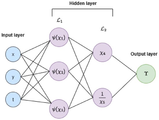
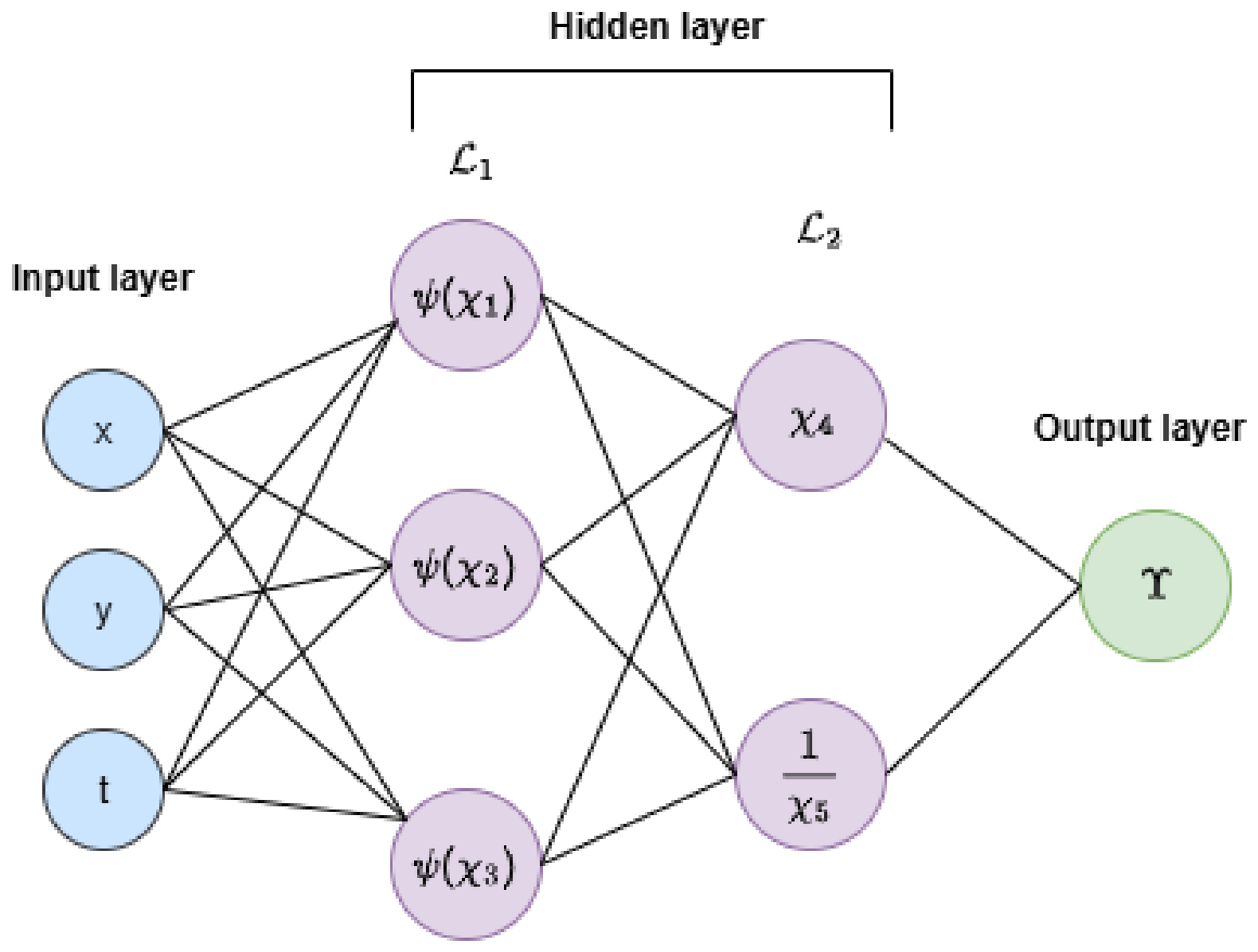
To construct analytical solutions of the K-II-X-E equation, we employ the neural network model shown in Figure 2, consisting of two hidden layers with three neurons. In the first hidden layer, the activation function $\psi (·)$ is applied to each neuron. The outputs of this layer are then propagated to the second hidden layer, where two different activation operations are used: an identity map $(·)$ and a reciprocal transformation $1/(·)$.

Figure 2. Architecture of NNs 1.

Based on this fixed network architecture, the trial solution $\mathrm{{\rm Y}}(x,y,t)$ is obtained by explicitly writing the forward propagation of the network in symbolic form, yielding

$$\begin{array}{cc}\hfill \hspace{1em}& \mathrm{{\rm Y}}(x,y,t)=\left(w_{13}\psi \left({\chi }_1\right)+w_{23}\psi \left({\chi }_2\right)+w_{33}\psi \left({\chi }_3\right)\right)w_{3\mathrm{{\rm Y}}}+{\displaystyle \frac{w_{4\mathrm{{\rm Y}}}}{w_{14}\psi \left({\chi }_1\right)+w_{24}\psi \left({\chi }_2\right)+w_{34}\psi \left({\chi }_3\right)}}+b,\hfill \end{array}$$

(6)

where ${\chi }_i=t{w}_{ti}+x{w}_{xi}+y{w}_{yi}$ for $i=1,2,3$.

Upon substituting Equation (6) into Equation (5), all derivatives of $\mathrm{{\rm Y}}(x,y,t)$ are computed, and the resulting expression is expanded. The equation is then reorganized in terms of a set of linearly independent basis functions given by

$$\begin{array}{c}\hfill \{x,y,t,\psi \left({\chi }_1\right),\psi \left({\chi }_2\right),\psi \left({\chi }_3\right)\}.\end{array}$$

Since these functions are assumed to be linearly independent over the considered domain, the only way for the resulting expression to hold identically for all $(x,y,t)$ is for the coefficients of each basis function to vanish. This procedure yields an underdetermined system of nonlinear algebraic equations for the unknown network parameters. A particular solution to this system, which determines the network’s weights and biases, is given by the following equation:

Set 1:

$$\begin{array}{cc}\hfill [\alpha & =-{\displaystyle \frac{w_{t3}\left(-4\breve{\kappa }{w}_{x3}^3+\beta w_{x3}+\mu w_{y3}+w_{t3}\right)}{w_{x3}^2}},\hspace{1em}b=b,\hspace{1em}\beta =\beta ,\hspace{1em}\breve{\kappa }=\breve{\kappa },\hspace{1em}\breve{\lambda }=0,\hspace{1em}\mu =\mu ,\hspace{1em}{w}_{13}=0,\hspace{1em}{w}_{14}=0,\hspace{1em}{w}_{23}=0,\hfill \\ \hfill \hspace{1em}& w_{24}=0,\hspace{1em}{w}_{33}=0,\hspace{1em}{w}_{34}={\displaystyle \frac{w_{4q}}{2\breve{\kappa }{w}_{x3}}},\hspace{1em}{w}_{t1}=w_{t1},\hspace{1em}{w}_{t2}=w_{t2},\hspace{1em}{w}_{t3}=w_{t3},\hspace{1em}{w}_{x1}=w_{x1},\hspace{1em}{w}_{x2}=w_{x2},\hspace{1em}{w}_{x3}=w_{x3},\hfill \\ \hfill \hspace{1em}& w_{y1}=w_{y1},\hspace{1em}{w}_{y2}=w_{y2},\hspace{1em}{w}_{y3}=w_{y3},\hspace{1em}{w}_{3\mathrm{{\rm Y}}}=w_{3\mathrm{{\rm Y}}},\hspace{1em}{w}_{4\mathrm{{\rm Y}}}=w_{4\mathrm{{\rm Y}}}].\hfill \end{array}$$

(7)

New exact analytical solutions are derived by inserting Equation (7) into Equation (6):

$${\mathrm{{\rm Y}}}_{i,j}^{\mathrm{K}-\mathrm{II}-\mathrm{X}-\mathrm{E}, \left(k\right)}(x,y,t)={\displaystyle \frac{2\breve{\kappa }{w}_{x3}}{\psi \left(t{w}_{t3}+x{w}_{x3}+y{w}_{y3}\right)}}+b,$$

(8)

where k, i, and j denote the case number, set number, and solution index within the set, respectively; $(x,y,t)$ are the independent variables of the K-II-X-E equation.

When $\breve{\kappa }<0$,

$${\mathrm{{\rm Y}}}_{1,1}^{\mathrm{K}-\mathrm{II}-\mathrm{X}-\mathrm{E}, \left(1\right)}={\displaystyle \frac{2\breve{\kappa }{w}_{x3}\left({\breve{S}}_1\cosh (\sqrt{-\breve{\kappa }} {\chi }_3)+{\breve{S}}_2\sinh (\sqrt{-\breve{\kappa }} {\chi }_3)\right)}{\sqrt{-\breve{\kappa }}\left({\breve{S}}_1\sinh (\sqrt{-\breve{\kappa }} {\chi }_3)+{\breve{S}}_2\cosh (\sqrt{-\breve{\kappa }} {\chi }_3)\right)}}+b.$$

(9)

When $\breve{\kappa }>0$,

$${\mathrm{{\rm Y}}}_{1,2}^{\mathrm{K}-\mathrm{II}-\mathrm{X}-\mathrm{E}, \left(1\right)}={\displaystyle \frac{2\sqrt{\breve{\kappa }} w_{x3}\left({\breve{S}}_1\cos (\sqrt{\breve{\kappa }} {\chi }_3)+{\breve{S}}_2\sin (\sqrt{\breve{\kappa }} {\chi }_3)\right)}{-{\breve{S}}_1\sin (\sqrt{\breve{\kappa }} {\chi }_3)+{\breve{S}}_2\cos (\sqrt{\breve{\kappa }} {\chi }_3)}}+b,$$

(10)

where ${\chi }_3=t{w}_{t3}+x{w}_{x3}+y{w}_{y3}$. Moreover, ${\breve{\mathcal{S}}}_1$ and ${\breve{\mathcal{S}}}_2$ are constants.

Set 2:

$$\begin{array}{cc}\hfill [\alpha & =-{\displaystyle \frac{w_{t3}\left(-4\breve{\kappa }{w}_{x3}^3+\beta w_{x3}+\mu w_{y3}+w_{t3}\right)}{w_{x3}^2}},\hspace{1em}b=b,\hspace{1em}\beta =\beta ,\hspace{1em}\breve{\kappa }=\breve{\kappa },\hspace{1em}\breve{\lambda }=0,\hspace{1em}\mu =\mu ,\hspace{1em}{w}_{13}=0,\hfill \\ \hfill \hspace{1em}& w_{14}=0,\hspace{1em}{w}_{23}=0,\hspace{1em}{w}_{24}=w_{24},\hspace{1em}{w}_{33}=0,\hspace{1em}{w}_{34}=w_{34},\hspace{1em}{w}_{t1}=w_{t1},\hspace{1em}{w}_{t2}=-{\displaystyle \frac{w_{24}{w}_{t3}}{w_{34}}},\hspace{1em}{w}_{t3}=w_{t3},\hfill \\ \hfill \hspace{1em}& w_{x1}=w_{x1},\hspace{1em}{w}_{x2}=-{\displaystyle \frac{w_{24}{w}_{x3}}{w_{34}}},\hspace{1em}{w}_{x3}=w_{x3},\hspace{1em}{w}_{y1}=w_{y1},\hspace{1em}{w}_{y2}=-{\displaystyle \frac{w_{24}\left(4\breve{\kappa }{w}_{24}^2{w}_{x3}^3-4\breve{\kappa }{w}_{34}^2{w}_{x3}^3+\mu w_{34}^2{w}_{y3}\right)}{\mu w_{34}^3}},\hfill \\ \hfill \hspace{1em}& w_{y3}=w_{y3},\hspace{1em}{w}_{3\mathrm{{\rm Y}}}=w_{3\mathrm{{\rm Y}}},\hspace{1em}{w}_{4\mathrm{{\rm Y}}}=-{\displaystyle \frac{2\breve{\kappa }{w}_{x3}\left(w_{24}^2-w_{34}^2\right)}{w_{34}}}].\hfill \end{array}$$

(11)

By inserting the result from Equation (11) into Equation (6), we obtain a new exact analytical solution:

$$\mathrm{{\rm Y}}(x,y,t)=-{\displaystyle \frac{2\breve{\kappa }{w}_{x3}\left(w_{24}^2-w_{34}^2\right)}{w_{34}\left[w_{24} \psi \left({\mathcal{R}}_1\right)+w_{34} \psi \left(t{w}_{t3}+x{w}_{x3}+y{w}_{y3}\right)\right]}}+b,$$

(12)

where ${\mathcal{R}}_1=-{\displaystyle \frac{t{w}_{24}{w}_{t3}}{w_{34}}}-{\displaystyle \frac{x{w}_{24}{w}_{x3}}{w_{34}}}-{\displaystyle \frac{y{w}_{24}\left(4\breve{\kappa }{w}_{24}^2{w}_{x3}^3-4\breve{\kappa }{w}_{34}^2{w}_{x3}^3+\mu w_{34}^2{w}_{y3}\right)}{\mu w_{34}^3}}$.

When $\breve{\kappa }<0$,

$${\mathrm{{\rm Y}}}_{2,1}^{\mathrm{K}-\mathrm{II}-\mathrm{X}-\mathrm{E}, \left(1\right)}=-{\displaystyle \frac{2\breve{\kappa } w_{x3}\left(w_{24}^2-w_{34}^2\right)}{w_{34}\left(\mathcal{A}+\mathcal{B}\right)}}+b,$$

(13)

where

$$\begin{array}{c}\hfill \mathcal{A}={\displaystyle \frac{w_{24}\sqrt{-\breve{\kappa }}\left({\breve{S}}_1\sinh (\sqrt{-\breve{\kappa }} {\mathcal{R}}_1)+{\breve{S}}_2\cosh (\sqrt{-\breve{\kappa }} {\mathcal{R}}_1)\right)}{{\breve{S}}_1\cosh (\sqrt{-\breve{\kappa }} {\mathcal{R}}_1)+{\breve{S}}_2\sinh (\sqrt{-\breve{\kappa }} {\mathcal{R}}_1)}},\end{array}$$

and 

$$\begin{array}{c}\hfill \mathcal{B}={\displaystyle \frac{w_{34}\sqrt{-\breve{\kappa }}\left({\breve{S}}_1\sinh (\sqrt{-\breve{\kappa }} {\chi }_3)+{\breve{S}}_2\cosh (\sqrt{-\breve{\kappa }} {\chi }_3)\right)}{{\breve{S}}_1\cosh (\sqrt{-\breve{\kappa }} {\chi }_3)+{\breve{S}}_2\sinh (\sqrt{-\breve{\kappa }} {\chi }_3)}}.\end{array}$$

When $\breve{\kappa }>0$,

$${\mathrm{{\rm Y}}}_{2,2}^{\mathrm{K}-\mathrm{II}-\mathrm{X}-\mathrm{E}, \left(1\right)}=-{\displaystyle \frac{2\breve{\kappa } w_{x3}\left(w_{24}^2-w_{34}^2\right)}{w_{34}\left(\mathcal{C}+\mathcal{D}\right)}}+b,$$

(14)

where 

$$\begin{array}{c}\hfill \mathcal{C}={\displaystyle \frac{w_{24}\sqrt{\breve{\kappa }}\left(-{\breve{S}}_1\sin (\sqrt{\breve{\kappa }} {\mathcal{R}}_1)+{\breve{S}}_2\cos (\sqrt{\breve{\kappa }} {\mathcal{R}}_1)\right)}{{\breve{S}}_1\cos (\sqrt{\breve{\kappa }} {\mathcal{R}}_1)+{\breve{S}}_2\sin (\sqrt{\breve{\kappa }} {\mathcal{R}}_1)}},\end{array}$$

and 

$$\begin{array}{c}\hfill \mathcal{D}={\displaystyle \frac{w_{34}\sqrt{\breve{\kappa }}\left(-{\breve{S}}_1\sin (\sqrt{\breve{\kappa }} {\chi }_3)+{\breve{S}}_2\cos (\sqrt{\breve{\kappa }} {\chi }_3)\right)}{{\breve{S}}_1\cos (\sqrt{\breve{\kappa }} {\chi }_3)+{\breve{S}}_2\sin (\sqrt{\breve{\kappa }} {\chi }_3)}},\end{array}$$

where ${\chi }_3=t{w}_{t3}+x{w}_{x3}+y{w}_{y3}$. Moreover, ${\breve{\mathcal{S}}}_1$ and ${\breve{\mathcal{S}}}_2$ are constants.

Set 3:

$$\begin{array}{cc}\hfill [\alpha & =-{\displaystyle \frac{6w_{t3}\breve{\kappa }{w}_{t2}{w}_{x3}\left(w_{24}^2-w_{34}^2\right)}{w_{34}\left(w_{24}{w}_{t3}+w_{34}{w}_{t2}\right)}},\hspace{1em}b=b,\hspace{1em}\beta =\beta ,\hspace{1em}\breve{\kappa }=\breve{\kappa },\hspace{1em}\breve{\lambda }=0,\hspace{1em}{w}_{23}=0,\hspace{1em}{w}_{24}=w_{24},\hspace{1em}{w}_{33}=0,\hfill \\ \hfill \hspace{1em}& \mu =-{\displaystyle \frac{-6\breve{\kappa }{w}_{24}^2{w}_{t2}{w}_{x3}^3-4\breve{\kappa }{w}_{24}{w}_{34}{w}_{t3}{w}_{x3}^3+2\breve{\kappa }{w}_{34}^2{w}_{t2}{w}_{x3}^3+\beta w_{24}{w}_{34}{w}_{t3}{w}_{x3}+\beta w_{34}^2{w}_{t2}{w}_{x3}+w_{24}{w}_{34}{w}_{t3}^2+w_{34}^2{w}_{t2}{w}_{t3}}{\left(w_{24}{w}_{t3}+w_{34}{w}_{t2}\right)w_{34}{w}_{y3}}},\hfill \\ \hfill \hspace{1em}& w_{13}=0,\hspace{1em}{w}_{14}=0,\hspace{1em}{w}_{34}=w_{34},\hspace{1em}{w}_{t1}=w_{t1},\hspace{1em}{w}_{t2}=w_{t2},\hspace{1em}{w}_{t3}=w_{t3},\hspace{1em}{w}_{x1}=w_{x1},\hspace{1em}{w}_{x2}=-{\displaystyle \frac{w_{24}{w}_{x3}}{w_{34}}},\hspace{1em}{w}_{x3}=w_{x3},\hfill \\ \hfill \hspace{1em}& w_{y2}=-{\displaystyle \frac{w_{y3}N}{w_{34}^{2}D}},\hspace{1em}{w}_{y3}=w_{y3},\hspace{1em}{w}_{3\mathrm{{\rm Y}}}=w_{3\mathrm{{\rm Y}}},\hspace{1em}{w}_{4\mathrm{{\rm Y}}}=-{\displaystyle \frac{2\breve{\kappa }{w}_{x3}\left(w_{24}^2-w_{34}^2\right)}{w_{34}}},\hspace{1em}{w}_{y1}=w_{y1}],\hfill \end{array}$$

(15)

where 

$$\begin{array}{cc}\hfill N& =2\breve{\kappa }{w}_{24}^4{w}_{t3}{w}_{x3}^3-4\breve{\kappa }{w}_{24}^3{w}_{34}{w}_{t2}{w}_{x3}^3-6\breve{\kappa }{w}_{24}^2{w}_{34}^2{w}_{t3}{w}_{x3}^3+\beta w_{24}^2{w}_{34}^2{w}_{t3}{w}_{x3}+\beta w_{24}{w}_{34}^3{w}_{t2}{w}_{x3}\hfill \\ \hfill \hspace{1em}& \hspace{1em}-w_{24}{w}_{34}^3{w}_{t2}{w}_{t3}-w_{34}^4{w}_{t2}^2,\hfill \\ \hfill D& =-6\breve{\kappa }{w}_{24}^2{w}_{t2}{w}_{x3}^3-4\breve{\kappa }{w}_{24}{w}_{34}{w}_{t3}{w}_{x3}^3+2\breve{\kappa }{w}_{34}^2{w}_{t2}{w}_{x3}^3+\beta w_{24}{w}_{34}{w}_{t3}{w}_{x3}+\beta w_{34}^2{w}_{t2}{w}_{x3}\hfill \\ \hfill \hspace{1em}& \hspace{1em}+w_{24}{w}_{34}{w}_{t3}^2+w_{34}^2{w}_{t2}{w}_{t3}.\hfill \end{array}$$

By inserting Equation (15) back into the trial solution Equation (6), we obtained the following:

$$\begin{array}{cc}\hfill \mathrm{{\rm Y}}(x,y,t)& =-{\displaystyle \frac{2\breve{\kappa }{w}_{x3}\left(w_{24}^2-w_{34}^2\right)}{w_{34}\left(w_{24} \psi \left({\mathcal{R}}_2\right)+w_{34} \psi \left(t{w}_{t3}+x{w}_{x3}+y{w}_{y3}\right)\right)}}+b,\hfill \end{array}$$

(16)

where 

$$\begin{array}{c}\hfill {\mathcal{R}}_2=t{w}_{t2}-{\displaystyle \frac{x{w}_{24}{w}_{x3}}{w_{34}}}-{\displaystyle \frac{y{w}_{y3}\mathcal{P}}{w_{34}^2\mathcal{Q}}},\end{array}$$

with 

$$\begin{array}{c}\hfill \mathcal{P}=2\breve{\kappa }{w}_{24}^4{w}_{t3}{w}_{x3}^3-4\breve{\kappa }{w}_{24}^3{w}_{34}{w}_{t2}{w}_{x3}^3-6\breve{\kappa }{w}_{24}^2{w}_{34}^2{w}_{t3}{w}_{x3}^3+\beta w_{24}^2{w}_{34}^2{w}_{t3}{w}_{x3}+\beta w_{24}{w}_{34}^3{w}_{t2}{w}_{x3}-w_{24}{w}_{34}^3{w}_{t2}{w}_{t3}-w_{34}^4{w}_{t2}^2,\end{array}$$

and 

$$\begin{array}{c}\hfill \mathcal{Q}=-6\breve{\kappa }{w}_{24}^2{w}_{t2}{w}_{x3}^3-4\breve{\kappa }{w}_{24}{w}_{34}{w}_{t3}{w}_{x3}^3+2\breve{\kappa }{w}_{34}^2{w}_{t2}{w}_{x3}^3+\beta w_{24}{w}_{34}{w}_{t3}{w}_{x3}+\beta w_{34}^2{w}_{t2}{w}_{x3}+w_{24}{w}_{34}{w}_{t3}^2+w_{34}^2{w}_{t2}{w}_{t3}.\end{array}$$

When $\breve{\kappa }<0$,

$${\mathrm{{\rm Y}}}_{3,1}^{\mathrm{K}-\mathrm{II}-\mathrm{X}-\mathrm{E}, \left(1\right)}=-{\displaystyle \frac{2\breve{\kappa } w_{x3}\left(w_{24}^2-w_{34}^2\right)}{w_{34}\left(\mathcal{G}+\mathcal{H}\right)}}+b,$$

(17)

where 

$$\begin{array}{c}\hfill \mathcal{G}={\displaystyle \frac{w_{24}\sqrt{-\breve{\kappa }}\left({\breve{S}}_1\sinh (\sqrt{-\breve{\kappa }} {\mathcal{R}}_2)+{\breve{S}}_2\cosh (\sqrt{-\breve{\kappa }} {\mathcal{R}}_2)\right)}{{\breve{S}}_1\cosh (\sqrt{-\breve{\kappa }} {\mathcal{R}}_2)+{\breve{S}}_2\sinh (\sqrt{-\breve{\kappa }} {\mathcal{R}}_2)}},\end{array}$$

and 

$$\begin{array}{c}\hfill \mathcal{H}={\displaystyle \frac{w_{34}\sqrt{-\breve{\kappa }}\left({\breve{S}}_1\sinh (\sqrt{-\breve{\kappa }} {\chi }_3)+{\breve{S}}_2\cosh (\sqrt{-\breve{\kappa }} {\chi }_3)\right)}{{\breve{S}}_1\cosh (\sqrt{-\breve{\kappa }} {\chi }_3)+{\breve{S}}_2\sinh (\sqrt{-\breve{\kappa }} {\chi }_3)}}.\end{array}$$

When $\breve{\kappa }>0$,

$${\mathrm{{\rm Y}}}_{3,2}^{\mathrm{K}-\mathrm{II}-\mathrm{X}-\mathrm{E}, \left(1\right)}=-{\displaystyle \frac{2\breve{\kappa } w_{x3}\left(w_{24}^2-w_{34}^2\right)}{w_{34}\left(\mathcal{A}+\mathcal{B}\right)}}+b,$$

(18)

where 

$$\begin{array}{c}\hfill \mathcal{A}={\displaystyle \frac{w_{24}\sqrt{\breve{\kappa }}\left(-{\breve{S}}_1\sin (\sqrt{\breve{\kappa }} {\mathcal{R}}_2)+{\breve{S}}_2\cos (\sqrt{\breve{\kappa }} {\mathcal{R}}_2)\right)}{{\breve{S}}_1\cos (\sqrt{\breve{\kappa }} {\mathcal{R}}_2)+{\breve{S}}_2\sin (\sqrt{\breve{\kappa }} {\mathcal{R}}_2)}},\end{array}$$

and 

$$\begin{array}{c}\hfill \mathcal{B}={\displaystyle \frac{w_{34}\sqrt{\breve{\kappa }}\left(-{\breve{S}}_1\sin (\sqrt{\breve{\kappa }} {\chi }_3)+{\breve{S}}_2\cos (\sqrt{\breve{\kappa }} {\chi }_3)\right)}{{\breve{S}}_1\cos (\sqrt{\breve{\kappa }} {\chi }_3)+{\breve{S}}_2\sin (\sqrt{\breve{\kappa }} {\chi }_3)}}.\end{array}$$

where ${\chi }_3=t{w}_{t3}+x{w}_{x3}+y{w}_{y3}$. Moreover, ${\breve{\mathcal{S}}}_1$ and ${\breve{\mathcal{S}}}_2$ are constants.

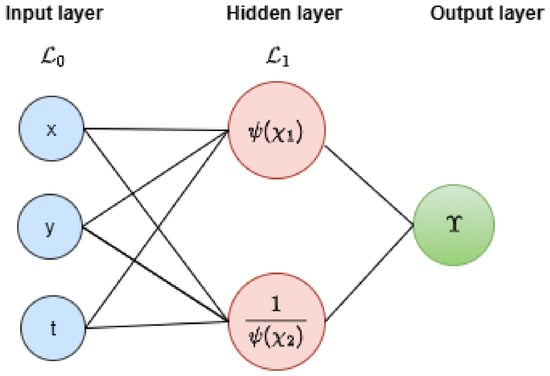
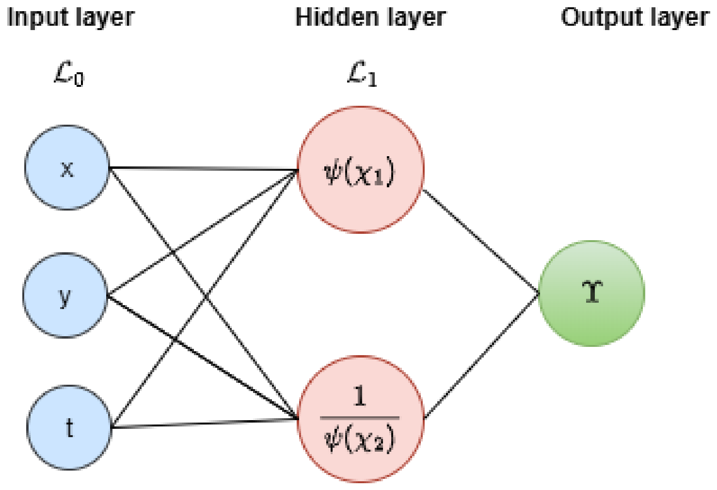
Figure 3 shows the versatility of the method by its implementation with different NN architectures for the solving of equations.

Figure 3. Architecture of NNs 2.

Case 2.

The analytical solution for Equation (5) is derived by a second NN solution, shown in Figure 3. Characteristics of this network are the following: Single hidden layer with two neurons. The input data to the first neuron in this layer is passed through the activation function $\psi (·)$, and the input data in the second layer is passed through $1/\psi (·)$, respectively. From this configuration, the trial function is derived:

$$\mathrm{{\rm Y}}(x,y,t)=w_{1\mathrm{{\rm Y}}}\psi (t{w}_{t1}+x{w}_{x1}+y{w}_{y1})+{\displaystyle \frac{w_{2\mathrm{{\rm Y}}}}{\psi (t{w}_{t2}+x{w}_{x2}+y{w}_{y2})}}+b_1,$$

(19)

applying the proposed method, we substitute the trial function from Equation (19) into the governing Equation (5) to derive the following solutions:

Set 1:

$$\begin{array}{cc}\hfill [\alpha & =-{\displaystyle \frac{w_{t2}\left(-{\breve{\lambda }}^2{w}_{x1}^3{w}_{x2}+{\breve{\lambda }}^2{w}_{x1}{w}_{x2}^3+4\breve{\kappa }{w}_{x1}^3{w}_{x2}-4\breve{\kappa }{w}_{x1}{w}_{x2}^3+\mu w_{x1}{w}_{y2}-\mu w_{x2}{w}_{y1}+2w_{t2}{w}_{x1}\right)}{2w_{x1}{w}_{x2}^2}},\hspace{1em}\mu =\mu \hfill \\ \hfill \beta & ={\displaystyle \frac{-{\breve{\lambda }}^2{w}_{x1}^3{w}_{x2}-{\breve{\lambda }}^2{w}_{x1}{w}_{x2}^3+4\breve{\kappa }{w}_{x1}^3{w}_{x2}+4\breve{\kappa }{w}_{x1}{w}_{x2}^3-\mu w_{x1}{w}_{y2}-\mu w_{x2}{w}_{y1}}{2w_{x1}{w}_{x2}}},\hspace{1em}\breve{\kappa }=\breve{\kappa },\hspace{1em}\breve{\lambda }=\breve{\lambda },\hspace{1em}{w}_{1\mathrm{{\rm Y}}}=-2w_{x1},\hfill \\ \hfill \hspace{1em}& w_{t1}=-{\displaystyle \frac{w_{t2}{w}_{x1}}{w_{x2}}},\hspace{1em}{w}_{t2}=w_{t2},\hspace{1em}{w}_{x1}=w_{x1},\hspace{1em}{w}_{x2}=w_{x2},\hspace{1em}{w}_{y1}=w_{y1},\hspace{1em}{w}_{y2}=w_{y2},\hspace{1em}{w}_{2\mathrm{{\rm Y}}}=2\breve{\kappa }{w}_{x2}].\hfill \end{array}$$

(20)

The final form of the novel exact solution is achieved by applying the parameters defined in Equation (20) to the structure provided by Equation (19):

$$\mathrm{{\rm Y}}(x,y,t)=-2w_{x1} \psi \left(-{\displaystyle \frac{t{w}_{t2}{w}_{x1}}{w_{x2}}}+x{w}_{x1}+y{w}_{y1}\right)+{\displaystyle \frac{2\breve{\kappa }{w}_{x2}}{\psi \left(t{w}_{t2}+x{w}_{x2}+y{w}_{y2}\right)}}+b_1.$$

(21)

When ${\breve{\lambda }}^2-4\breve{\kappa }>0$,

$$\begin{array}{cc}\hfill {\mathrm{{\rm Y}}}_{1,1}^{\mathrm{K}-\mathrm{II}-\mathrm{X}-\mathrm{E}, \left(2\right)}& =-2w_{x1} \left(-{\displaystyle \frac{\breve{\lambda }}{2}}+{\displaystyle \frac{\sqrt{{\breve{\lambda }}^2-4\breve{\kappa }}\left({\breve{\mathcal{S}}}_1\sinh \left(\frac{1}{2}\sqrt{{\breve{\lambda }}^2-4\breve{\kappa }} {\mathrm{K}}_1\right)+{\breve{\mathcal{S}}}_2\cosh \left(\frac{1}{2}\sqrt{{\breve{\lambda }}^2-4\breve{\kappa }} {\mathrm{K}}_1\right)\right)}{2\left({\breve{\mathcal{S}}}_1\cosh \left(\frac{1}{2}\sqrt{{\breve{\lambda }}^2-4\breve{\kappa }} {\mathrm{K}}_1\right)+{\breve{\mathcal{S}}}_2\sinh \left(\frac{1}{2}\sqrt{{\breve{\lambda }}^2-4\breve{\kappa }} {\mathrm{K}}_1\right)\right)}}\right)\hfill \\ \hfill \hspace{1em}& \hspace{1em}+{\displaystyle \frac{2\breve{\kappa }{w}_{x2}}{\left(-\frac{\breve{\lambda }}{2}+\frac{\sqrt{{\breve{\lambda }}^2-4\breve{\kappa }}\left({\breve{\mathcal{S}}}_1\sinh \left(\frac{1}{2}\sqrt{{\breve{\lambda }}^2-4\breve{\kappa }} {\chi }_2\right)+{\breve{\mathcal{S}}}_2\cosh \left(\frac{1}{2}\sqrt{{\breve{\lambda }}^2-4\breve{\kappa }} {\chi }_2\right)\right)}{2\left({\breve{\mathcal{S}}}_1\cosh \left(\frac{1}{2}\sqrt{{\breve{\lambda }}^2-4\breve{\kappa }} {\chi }_2\right)+{\breve{\mathcal{S}}}_2\sinh \left(\frac{1}{2}\sqrt{{\breve{\lambda }}^2-4\breve{\kappa }} {\chi }_2\right)\right)}\right)}}+b_1.\hfill \end{array}$$

(22)

When ${\breve{\lambda }}^2-4\breve{\kappa }<0$,

$$\begin{array}{cc}\hfill {\mathrm{{\rm Y}}}_{1,2}^{\mathrm{K}-\mathrm{II}-\mathrm{X}-\mathrm{E}, \left(2\right)}& =-2w_{x1} \left(-{\displaystyle \frac{\breve{\lambda }}{2}}+{\displaystyle \frac{\sqrt{4\breve{\kappa }-{\breve{\lambda }}^2}\left(-{\breve{\mathcal{S}}}_1\sin \left(\frac{1}{2}\sqrt{4\breve{\kappa }-{\breve{\lambda }}^2} {\mathrm{K}}_1\right)+{\breve{\mathcal{S}}}_2\cos \left(\frac{1}{2}\sqrt{4\breve{\kappa }-{\breve{\lambda }}^2} {\mathrm{K}}_1\right)\right)}{2\left({\breve{\mathcal{S}}}_1\cos \left(\frac{1}{2}\sqrt{4\breve{\kappa }-{\breve{\lambda }}^2} {\mathrm{K}}_1\right)+{\breve{\mathcal{S}}}_2\sin \left(\frac{1}{2}\sqrt{4\breve{\kappa }-{\breve{\lambda }}^2} {\mathrm{K}}_1\right)\right)}}\right)\hfill \\ \hfill \hspace{1em}& \hspace{1em}+{\displaystyle \frac{2\breve{\kappa }{w}_{x2}}{\left(-\frac{\breve{\lambda }}{2}+\frac{\sqrt{4\breve{\kappa }-{\breve{\lambda }}^2}\left(-{\breve{\mathcal{S}}}_1\sin \left(\frac{1}{2}\sqrt{4\breve{\kappa }-{\breve{\lambda }}^2} {\chi }_2\right)+{\breve{\mathcal{S}}}_2\cos \left(\frac{1}{2}\sqrt{4\breve{\kappa }-{\breve{\lambda }}^2} {\chi }_2\right)\right)}{2\left({\breve{\mathcal{S}}}_1\cos \left(\frac{1}{2}\sqrt{4\breve{\kappa }-{\breve{\lambda }}^2} {\chi }_2\right)+{\breve{\mathcal{S}}}_2\sin \left(\frac{1}{2}\sqrt{4\breve{\kappa }-{\breve{\lambda }}^2} {\chi }_2\right)\right)}\right)}}+b_1.\hfill \end{array}$$

(23)

When ${\breve{\lambda }}^2-4\breve{\kappa }=0$,

$${\mathrm{{\rm Y}}}_{1,3}^{\mathrm{K}-\mathrm{II}-\mathrm{X}-\mathrm{E}, \left(2\right)}=-2w_{x1}\left(-\sqrt{\breve{\kappa }}+{\displaystyle \frac{{\breve{S}}_2}{{\breve{S}}_1+{\breve{S}}_2{\mathrm{K}}_1}}\right)+{\displaystyle \frac{2\breve{\kappa } w_{x2}}{-\sqrt{\breve{\kappa }}+{\displaystyle \frac{{\breve{S}}_2}{{\breve{S}}_1+{\breve{S}}_2{\chi }_2}}}}+b_1,$$

(24)

where ${\mathrm{K}}_1=-{\displaystyle \frac{t{w}_{t2}{w}_{x1}}{w_{x2}}}+x{w}_{x1}+y{w}_{y1}$, ${\chi }_2=t{w}_{t2}+x{w}_{x2}+y{w}_{y2}$. Moreover, ${\breve{\mathcal{S}}}_1$ and ${\breve{\mathcal{S}}}_2$ are constants.

Set 2:

$$\begin{array}{cc}\hfill [& \alpha =-{\displaystyle \frac{w_{t1}\left({\breve{\kappa }}^2{w}_{x1}^3-4\breve{\lambda }{w}_{x1}^3+\beta w_{x1}+\mu w_{y1}+w_{t1}\right)}{w_{x1}^2}},\hspace{1em}\beta =\beta ,\hspace{1em}\breve{\lambda }=\breve{\lambda },\hspace{1em}\breve{\kappa }=\breve{\kappa },\hspace{1em}\mu =\mu ,\hspace{1em}{b}_1=b_1,\hspace{1em}{w}_{\mathrm{{\rm Y}}}=-2w_{x1},\hfill \\ \hfill \hspace{1em}& w_{t1}=w_{t1},\hspace{1em}{w}_{t2}=0,\hspace{1em}{w}_{x1}=w_{x1},\hspace{1em}{w}_{x2}=0,\hspace{1em}{w}_{y1}=w_{y1},\hspace{1em}{w}_{y2}=w_{y2},\hspace{1em}{w}_{2\mathrm{{\rm Y}}}=w_{2\mathrm{{\rm Y}}}].\hfill \end{array}$$

(25)

By substituting the determined coefficients from Equation (25) back into the trial function Equation (19), we arrive at the following:

$$\mathrm{{\rm Y}}(x,y,t)=-2w_{x1} \psi \left(t{w}_{t1}+x{w}_{x1}+y{w}_{y1}\right)+{\displaystyle \frac{w_{2\mathrm{{\rm Y}}}}{\psi \left(y{w}_{y2}\right)}}+b_1.$$

(26)

When ${\breve{\lambda }}^2-4\breve{\kappa }>0$,

$$\begin{array}{cc}\hfill {\mathrm{{\rm Y}}}_{2,1}^{\mathrm{K}-\mathrm{II}-\mathrm{X}-\mathrm{E}, \left(2\right)}& =-2w_{x1} \left(-{\displaystyle \frac{\breve{\lambda }}{2}}+{\displaystyle \frac{\sqrt{{\breve{\lambda }}^2-4\breve{\kappa }}\left({\breve{\mathcal{S}}}_1\sinh \left(\frac{1}{2}\sqrt{{\breve{\lambda }}^2-4\breve{\kappa }} {\chi }_1\right)+{\breve{\mathcal{S}}}_2\cosh \left(\frac{1}{2}\sqrt{{\breve{\lambda }}^2-4\breve{\kappa }} {\chi }_1\right)\right)}{2\left({\breve{\mathcal{S}}}_1\cosh \left(\frac{1}{2}\sqrt{{\breve{\lambda }}^2-4\breve{\kappa }} {\chi }_1\right)+{\breve{\mathcal{S}}}_2\sinh \left(\frac{1}{2}\sqrt{{\breve{\lambda }}^2-4\breve{\kappa }} {\chi }_1\right)\right)}}\right)\hfill \\ \hfill \hspace{1em}& \hspace{1em}+{\displaystyle \frac{w_{2\mathrm{{\rm Y}}}}{\left(-\frac{\breve{\lambda }}{2}+\frac{\sqrt{{\breve{\lambda }}^2-4\breve{\kappa }}\left({\breve{\mathcal{S}}}_1\sinh \left(\frac{1}{2}\sqrt{{\breve{\lambda }}^2-4\breve{\kappa }} {\chi }_2\right)+{\breve{\mathcal{S}}}_2\cosh \left(\frac{1}{2}\sqrt{{\breve{\lambda }}^2-4\breve{\kappa }} {\chi }_2\right)\right)}{2\left({\breve{\mathcal{S}}}_1\cosh \left(\frac{1}{2}\sqrt{{\breve{\lambda }}^2-4\breve{\kappa }} {\chi }_2\right)+{\breve{\mathcal{S}}}_2\sinh \left(\frac{1}{2}\sqrt{{\breve{\lambda }}^2-4\breve{\kappa }} {\chi }_2\right)\right)}\right)}}+b_1.\hfill \end{array}$$

(27)

When ${\breve{\lambda }}^2-4\breve{\kappa }<0$,

$$\begin{array}{cc}\hfill {\mathrm{{\rm Y}}}_{2,2}^{\mathrm{K}-\mathrm{II}-\mathrm{X}-\mathrm{E}, \left(2\right)}& =-2w_{x1} \left(-{\displaystyle \frac{\breve{\lambda }}{2}}+{\displaystyle \frac{\sqrt{4\breve{\kappa }-{\breve{\lambda }}^2}\left(-{\breve{\mathcal{S}}}_1\sin \left(\frac{1}{2}\sqrt{4\breve{\kappa }-{\breve{\lambda }}^2} {\chi }_1\right)+{\breve{\mathcal{S}}}_2\cos \left(\frac{1}{2}\sqrt{4\breve{\kappa }-{\breve{\lambda }}^2} {\chi }_1\right)\right)}{2\left({\breve{\mathcal{S}}}_1\cos \left(\frac{1}{2}\sqrt{4\breve{\kappa }-{\breve{\lambda }}^2} {\chi }_1\right)+{\breve{\mathcal{S}}}_2\sin \left(\frac{1}{2}\sqrt{4\breve{\kappa }-{\breve{\lambda }}^2} {\chi }_1\right)\right)}}\right)\hfill \\ \hfill \hspace{1em}& \hspace{1em}+{\displaystyle \frac{w_{2\mathrm{{\rm Y}}}}{\left(-\frac{\breve{\lambda }}{2}+\frac{\sqrt{4\breve{\kappa }-{\breve{\lambda }}^2}\left(-{\breve{\mathcal{S}}}_1\sin \left(\frac{1}{2}\sqrt{4\breve{\kappa }-{\breve{\lambda }}^2} {\chi }_2\right)+{\breve{\mathcal{S}}}_2\cos \left(\frac{1}{2}\sqrt{4\breve{\kappa }-{\breve{\lambda }}^2} {\chi }_2\right)\right)}{2\left({\breve{\mathcal{S}}}_1\cos \left(\frac{1}{2}\sqrt{4\breve{\kappa }-{\breve{\lambda }}^2} {\chi }_2\right)+{\breve{\mathcal{S}}}_2\sin \left(\frac{1}{2}\sqrt{4\breve{\kappa }-{\breve{\lambda }}^2} {\chi }_2\right)\right)}\right)}}+b_1.\hfill \end{array}$$

(28)

When ${\breve{\lambda }}^2-4\breve{\kappa }=0$,

$${\mathrm{{\rm Y}}}_{2,3}^{\mathrm{K}-\mathrm{II}-\mathrm{X}-\mathrm{E}, \left(2\right)}=-2w_{x1}\left(-\sqrt{\breve{\kappa }}+{\displaystyle \frac{{\breve{S}}_2}{{\breve{S}}_1+{\breve{S}}_2{\chi }_1}}\right)+{\displaystyle \frac{w_{2\mathrm{{\rm Y}}}}{-\sqrt{\breve{\kappa }}+{\displaystyle \frac{{\breve{S}}_2}{{\breve{S}}_1+{\breve{S}}_2{\chi }_2}}}}+b_1,$$

(29)

where ${\chi }_1=t{w}_{t1}+x{w}_{x1}+y{w}_{y1}$, ${\chi }_2=y{w}_{y2}$. Moreover, ${\breve{\mathcal{S}}}_1$ and ${\breve{\mathcal{S}}}_2$ are constants.

Set 3:

$$\begin{array}{cc}\hfill [& \alpha =-{\displaystyle \frac{w_{t2}\left({\kappa }^2{w}_{x2}^3-4\eta w_{x2}^3+\beta w_{x2}+\mu w_{y2}+w_{t2}\right)}{w_{x2}^2}},\hspace{1em}\beta =\beta ,\hspace{1em}\breve{\lambda }=\breve{\lambda },\hspace{1em}\breve{\kappa }=\breve{\kappa },\hspace{1em}\mu =\mu ,\hspace{1em}{b}_1=b_1,\hspace{1em}{w}_{1\mathrm{{\rm Y}}}=w_{1\mathrm{{\rm Y}}},\hfill \\ \hfill \hspace{1em}& w_{t1}=0,\hspace{1em}{w}_{t2}=w_{t2},\hspace{1em}{w}_{x1}=0,\hspace{1em}{w}_{x2}=w_{x2},\hspace{1em}{w}_{y1}=w_{y1},\hspace{1em}{w}_{y2}=w_{y2},\hspace{1em}{w}_{2\mathrm{{\rm Y}}}=2\breve{\kappa }{w}_{x2}].\hfill \end{array}$$

(30)

By substituting the determined coefficients from Equation (30) back into the trial function Equation (19), we arrive at the following:

$$\mathrm{{\rm Y}}(x,y,t)=w_{1\mathrm{{\rm Y}}} \psi \left(y{w}_{y1}\right)+{\displaystyle \frac{2\breve{\kappa } w_{x2}}{\psi \left(t w_{t2}+x w_{x2}+y w_{y2}\right)}}+b_1.$$

(31)

When ${\breve{\lambda }}^2-4\breve{\kappa }>0$,

$$\begin{array}{cc}\hfill {\mathrm{{\rm Y}}}_{3,1}^{\mathrm{K}-\mathrm{II}-\mathrm{X}-\mathrm{E}, \left(2\right)}& =w_{1\mathrm{{\rm Y}}}\left(-{\displaystyle \frac{\breve{\lambda }}{2}}+{\displaystyle \frac{\sqrt{{\breve{\lambda }}^2-4\breve{\kappa }}\left({\breve{\mathcal{S}}}_1\sinh \left(\frac{1}{2}\sqrt{{\breve{\lambda }}^2-4\breve{\kappa }} {\chi }_1\right)+{\breve{\mathcal{S}}}_2\cosh \left(\frac{1}{2}\sqrt{{\breve{\lambda }}^2-4\breve{\kappa }} {\chi }_1\right)\right)}{2\left({\breve{\mathcal{S}}}_1\cosh \left(\frac{1}{2}\sqrt{{\breve{\lambda }}^2-4\breve{\kappa }} {\chi }_1\right)+{\breve{\mathcal{S}}}_2\sinh \left(\frac{1}{2}\sqrt{{\breve{\lambda }}^2-4\breve{\kappa }} {\chi }_1\right)\right)}}\right)\hfill \\ \hfill \hspace{1em}& \hspace{1em}+{\displaystyle \frac{w_{2\mathrm{{\rm Y}}}}{\left(-\frac{\breve{\lambda }}{2}+\frac{\sqrt{{\breve{\lambda }}^2-4\breve{\kappa }}\left({\breve{\mathcal{S}}}_1\sinh \left(\frac{1}{2}\sqrt{{\breve{\lambda }}^2-4\breve{\kappa }} {\chi }_2\right)+{\breve{\mathcal{S}}}_2\cosh \left(\frac{1}{2}\sqrt{{\breve{\lambda }}^2-4\breve{\kappa }} {\chi }_2\right)\right)}{2\left({\breve{\mathcal{S}}}_1\cosh \left(\frac{1}{2}\sqrt{{\breve{\lambda }}^2-4\breve{\kappa }} {\chi }_2\right)+{\breve{\mathcal{S}}}_2\sinh \left(\frac{1}{2}\sqrt{{\breve{\lambda }}^2-4\breve{\kappa }} {\chi }_2\right)\right)}\right)}}+b_1.\hfill \end{array}$$

(32)

When ${\breve{\lambda }}^2-4\breve{\kappa }<0$,

$$\begin{array}{cc}\hfill {\mathrm{{\rm Y}}}_{3,2}^{\mathrm{K}-\mathrm{II}-\mathrm{X}-\mathrm{E}, \left(2\right)}& =w_{1\mathrm{{\rm Y}}}\left(-{\displaystyle \frac{\breve{\lambda }}{2}}+{\displaystyle \frac{\sqrt{4\breve{\kappa }-{\breve{\lambda }}^2}\left(-{\breve{\mathcal{S}}}_1\sin \left(\frac{1}{2}\sqrt{4\breve{\kappa }-{\breve{\lambda }}^2} {\chi }_1\right)+{\breve{\mathcal{S}}}_2\cos \left(\frac{1}{2}\sqrt{4\breve{\kappa }-{\breve{\lambda }}^2} {\chi }_1\right)\right)}{2\left({\breve{\mathcal{S}}}_1\cos \left(\frac{1}{2}\sqrt{4\breve{\kappa }-{\breve{\lambda }}^2} {\chi }_1\right)+{\breve{\mathcal{S}}}_2\sin \left(\frac{1}{2}\sqrt{4\breve{\kappa }-{\breve{\lambda }}^2} {\chi }_1\right)\right)}}\right)\hfill \\ \hfill \hspace{1em}& \hspace{1em}+{\displaystyle \frac{w_{2\mathrm{{\rm Y}}}}{\left(-\frac{\breve{\lambda }}{2}+\frac{\sqrt{4\breve{\kappa }-{\breve{\lambda }}^2}\left(-{\breve{\mathcal{S}}}_1\sin \left(\frac{1}{2}\sqrt{4\breve{\kappa }-{\breve{\lambda }}^2} {\chi }_2\right)+{\breve{\mathcal{S}}}_2\cos \left(\frac{1}{2}\sqrt{4\breve{\kappa }-{\breve{\lambda }}^2} {\chi }_2\right)\right)}{2\left({\breve{\mathcal{S}}}_1\cos \left(\frac{1}{2}\sqrt{4\breve{\kappa }-{\breve{\lambda }}^2} {\chi }_2\right)+{\breve{\mathcal{S}}}_2\sin \left(\frac{1}{2}\sqrt{4\breve{\kappa }-{\breve{\lambda }}^2} {\chi }_2\right)\right)}\right)}}+b_1.\hfill \end{array}$$

(33)

When ${\breve{\lambda }}^2-4\breve{\kappa }=0$,

$${\mathrm{{\rm Y}}}_{3,3}^{\mathrm{K}-\mathrm{II}-\mathrm{X}-\mathrm{E}, \left(2\right)}=w_{\mathrm{{\rm Y}}}\left(-\sqrt{\breve{\kappa }}+{\displaystyle \frac{{\breve{S}}_2}{{\breve{S}}_1+{\breve{S}}_2{\chi }_1}}\right)+{\displaystyle \frac{2\breve{\kappa } w_{x2}}{-\sqrt{\breve{\kappa }}+{\displaystyle \frac{{\breve{S}}_2}{{\breve{S}}_1+{\breve{S}}_2{\chi }_2}}}}+b_1,$$

(34)

where ${\chi }_1=y{w}_{y1}$, ${\chi }_2=t w_{t2}+x w_{x2}+y w_{y2}$. Moreover, ${\breve{\mathcal{S}}}_1$ and ${\breve{\mathcal{S}}}_2$ are constants.

3.2. The Kairat-II-X-Type Equation

The K-II-X equation, derived by dropping the term ${\mathrm{{\rm Y}}}_{tt}$ from the K-II-X-E Equation (5), is given by the following equation [60]:

$$\begin{array}{c}\hfill {\mathrm{{\rm Y}}}_{xxxt}-3{\left({\mathrm{{\rm Y}}}_x{\mathrm{{\rm Y}}}_t\right)}_x+\alpha {\mathrm{{\rm Y}}}_{xx}+\beta {\mathrm{{\rm Y}}}_x{\mathrm{{\rm Y}}}_t+\mu {\mathrm{{\rm Y}}}_{yt}=0,\end{array}$$

(35)

where $\mathrm{{\rm Y}}=\mathrm{{\rm Y}}(x,y,t)$ is as defined in (5). Clearly, the equation contains two nonlinear terms, namely $-3{\left({\mathrm{{\rm Y}}}_x{\mathrm{{\rm Y}}}_t\right)}_x$ and $\beta {\mathrm{{\rm Y}}}_x{\mathrm{{\rm Y}}}_t$, together with three linear terms given by ${\mathrm{{\rm Y}}}_{xxxt}$, $\alpha {\mathrm{{\rm Y}}}_{xx}$, and $\mu {\mathrm{{\rm Y}}}_{yt}$. It includes only one term involving partial derivatives with respect to y and t as introduced in (5).

Case 3.

To construct analytical solutions of the K-II-X-type equation, we employ the neural network model shown in Figure 2, consisting of two hidden layers with three neurons. In the first hidden layer, the activation function $\psi (·)$ is applied to each neuron. The outputs of this layer are then propagated to the second hidden layer, where two different activation operations are used: an identity map $(·)$ and a reciprocal transformation $1/(·)$.

Based on this fixed network architecture, the trial solution $\mathrm{{\rm Y}}(x,y,t)$ is obtained by explicitly writing the forward propagation of the network in symbolic form, yielding

$$\begin{array}{cc}\hfill \hspace{1em}& \mathrm{{\rm Y}}(x,y,t)=\left(w_{13}\psi \left({\chi }_1\right)+w_{23}\psi \left({\chi }_2\right)+w_{33}\psi \left({\chi }_3\right)\right)w_{3\mathrm{{\rm Y}}}+{\displaystyle \frac{w_{4\mathrm{{\rm Y}}}}{w_{14}\psi \left({\chi }_1\right)+w_{24}\psi \left({\chi }_2\right)+w_{34}\psi \left({\chi }_3\right)}}+b,\hfill \end{array}$$

(36)

where ${\chi }_i=t{w}_{ti}+x{w}_{xi}+y{w}_{yi}$ for $i=1,2,3$.

Upon substituting Equation (36) into Equation (35), all derivatives of $\mathrm{{\rm Y}}(x,y,t)$ are computed, and the resulting expression is expanded. The equation is then reorganized in terms of a set of linearly independent basis functions given by

$$\begin{array}{c}\hfill \{x,y,t,\psi \left({\chi }_1\right),\psi \left({\chi }_2\right),\psi \left({\chi }_3\right)\}.\end{array}$$

Since these functions are assumed to be linearly independent over the considered domain, the only way for the resulting expression to hold identically for all $(x,y,t)$ is for the coefficients of each basis function to vanish. This procedure yields an underdetermined system of nonlinear algebraic equations for the unknown network parameters. A particular solution to this system, which determines the network’s weights and biases, is given by the following equation:

Set 1:

$$\begin{array}{cc}\hfill [\alpha & ={\displaystyle \frac{w_{t2}\left(-6\breve{\kappa }{w}_{24}^2{w}_{x3}^2+2\breve{\kappa }{w}_{34}^2{w}_{x3}^2+\beta w_{34}^2\right)}{w_{34}{w}_{x3}{w}_{24}}},\hspace{1em}b=b,\hspace{1em}\beta =\beta ,\hspace{1em}\breve{\kappa }=\breve{\kappa },\hspace{1em}\breve{\lambda }=0,\hspace{1em}\mu =\mu ,\hspace{1em}{w}_{13}=0,\hspace{1em}{w}_{14}=0,\hspace{1em}{w}_{23}=0,\hfill \\ \hfill \hspace{1em}& w_{24}=w_{24},\hspace{1em}{w}_{33}=0,\hspace{1em}{w}_{34}=w_{34},\hspace{1em}{w}_{t1}=w_{t1},\hspace{1em}{w}_{t2}=w_{t2},\hspace{1em}{w}_{t3}=-{\displaystyle \frac{w_{t2}\left(-6\breve{\kappa }{w}_{24}^2{w}_{x3}^2+2\breve{\kappa }{w}_{34}^2{w}_{x3}^2+\beta w_{34}^2\right)}{w_{24}{w}_{34}\left(-4\breve{\kappa }{w}_{x3}^2+\beta \right)}},\hfill \\ \hfill \hspace{1em}& w_{x1}=w_{x1},\hspace{1em}{w}_{x2}=-{\displaystyle \frac{w_{24}{w}_{x3}}{w_{34}}},\hspace{1em}{w}_{x3}=w_{x3},\hspace{1em}{w}_{y1}=w_{y1},\hspace{1em}{w}_{y2}={\displaystyle \frac{2\left(w_{24}^2-w_{34}^2\right)w_{24}\breve{\kappa }{w}_{x3}^3}{\mu w_{34}^3}},\hspace{1em}{w}_{y3}=0,\hspace{1em}{w}_{3\mathrm{{\rm Y}}}=w_{3\mathrm{{\rm Y}}},\hfill \\ \hfill \hspace{1em}& w_{4\mathrm{{\rm Y}}}=-{\displaystyle \frac{2\breve{\kappa }{w}_{x3}\left(w_{24}^2-w_{34}^2\right)}{w_{34}}}].\hfill \end{array}$$

(37)

By inserting the results from Equation (37) into the structural form of Equation (36), we construct the following novel exact analytical solution:

$$\mathrm{{\rm Y}}(x,y,t)=-{\displaystyle \frac{2\breve{\kappa }{w}_{x3}\left(w_{24}^2-w_{34}^2\right)}{w_{34}\left(w_{24} \psi \left({\chi }_4\right)+w_{34} \psi \left({\chi }_5\right)\right)}}+b,$$

(38)

where

$$\begin{array}{cc}\hfill {\chi }_4& =t{w}_{t2}-{\displaystyle \frac{x{w}_{24}{w}_{x3}}{w_{34}}}+{\displaystyle \frac{2y\left(w_{24}^2-w_{34}^2\right)w_{24}\breve{\kappa }{w}_{x3}^3}{\mu w_{34}^3}},\hfill \\ \hfill {\chi }_5& =-{\displaystyle \frac{t{w}_{t2}\left(-6\breve{\kappa }{w}_{24}^2{w}_{x3}^2+2\breve{\kappa }{w}_{34}^2{w}_{x3}^2+\beta w_{34}^2\right)}{w_{24}{w}_{34}\left(-4\breve{\kappa }{w}_{x3}^2+\beta \right)}}+x{w}_{x3}.\hfill \end{array}$$

When $\breve{\kappa }<0$,

$${\mathrm{{\rm Y}}}_{1,1}^{\mathrm{K}-\mathrm{II}-\mathrm{X}, \left(1\right)}=-{\displaystyle \frac{2\breve{\kappa } w_{x3}\left(w_{24}^2-w_{34}^2\right)}{w_{34}\left(\mathcal{K}+\mathcal{L}\right)}}+b,$$

(39)

where

$$\begin{array}{c}\hfill \mathcal{K}={\displaystyle \frac{w_{24}\sqrt{-\breve{\kappa }}\left({\breve{S}}_1\sinh (\sqrt{-\breve{\kappa }} {\chi }_4)+{\breve{S}}_2\cosh (\sqrt{-\breve{\kappa }} {\chi }_4)\right)}{{\breve{S}}_1\cosh (\sqrt{-\breve{\kappa }} {\chi }_4)+{\breve{S}}_2\sinh (\sqrt{-\breve{\kappa }} {\chi }_4)}},\\ \hfill \mathcal{L}={\displaystyle \frac{w_{34}\sqrt{-\breve{\kappa }}\left({\breve{S}}_1\sinh (\sqrt{-\breve{\kappa }} {\chi }_5)+{\breve{S}}_2\cosh (\sqrt{-\breve{\kappa }} {\chi }_5)\right)}{{\breve{S}}_1\cosh (\sqrt{-\breve{\kappa }} {\chi }_5)+{\breve{S}}_2\sinh (\sqrt{-\breve{\kappa }} {\chi }_5)}}.\end{array}$$

When $\breve{\kappa }>0$,

$${\mathrm{{\rm Y}}}_{1,2}^{\mathrm{K}-\mathrm{II}-\mathrm{X}, \left(1\right)}=-{\displaystyle \frac{2\breve{\kappa } w_{x3}\left(w_{24}^2-w_{34}^2\right)}{w_{34}\left(\mathcal{M}+\mathcal{N}\right)}}+b,$$

(40)

where

$$\begin{array}{c}\hfill \mathcal{M}={\displaystyle \frac{w_{24}\sqrt{\breve{\kappa }}\left(-{\breve{S}}_1\sin (\sqrt{\breve{\kappa }} {\chi }_4)+{\breve{S}}_2\cos (\sqrt{\breve{\kappa }} {\chi }_4)\right)}{{\breve{S}}_1\cos (\sqrt{\breve{\kappa }} {\chi }_4)+{\breve{S}}_2\sin (\sqrt{\breve{\kappa }} {\chi }_4)}},\\ \hfill \mathcal{N}={\displaystyle \frac{w_{34}\sqrt{\breve{\kappa }}\left(-{\breve{S}}_1\sin (\sqrt{\breve{\kappa }} {\chi }_5)+{\breve{S}}_2\cos (\sqrt{\breve{\kappa }} {\chi }_5)\right)}{{\breve{S}}_1\cos (\sqrt{\breve{\kappa }} {\chi }_5)+{\breve{S}}_2\sin (\sqrt{\breve{\kappa }} {\chi }_5)}}.\end{array}$$

where ${\breve{\mathcal{S}}}_1$ and ${\breve{\mathcal{S}}}_2$ are constants.

Set 2:

$$\begin{array}{cc}\hfill [\alpha & =-{\displaystyle \frac{w_{t3}\left(-4\breve{\kappa }{w}_{x3}^3+\beta w_{x3}+\mu w_{y3}\right)}{w_{x3}^2}},\hspace{1em}b=b,\hspace{1em}\beta =\beta ,\hspace{1em}\breve{\kappa }=\breve{\kappa },\hspace{1em}\breve{\lambda }=0,\hspace{1em}\mu =\mu ,\hspace{1em}{w}_{13}=0,\hspace{1em}{w}_{14}=0,\hspace{1em}{w}_{23}=0,\hfill \\ \hfill \hspace{1em}& w_{24}=w_{24},\hspace{1em}{w}_{33}=0,\hspace{1em}{w}_{34}=w_{34},\hspace{1em}{w}_{t1}=w_{t1},\hspace{1em}{w}_{t2}=-{\displaystyle \frac{w_{t3}{w}_{24}}{w_{34}}},\hspace{1em}{w}_{t3}=w_{t3},\hspace{1em}{w}_{x1}=w_{x1},\hspace{1em}{w}_{x2}=-{\displaystyle \frac{w_{24}{w}_{x3}}{w_{34}}},\hfill \\ \hfill \hspace{1em}& w_{x3}=w_{x3},\hspace{1em}{w}_{y1}=w_{y1},\hspace{1em}{w}_{y2}=-{\displaystyle \frac{w_{24}\left(4\breve{\kappa }{w}_{24}^2{w}_{x3}^3-4\breve{\kappa }{w}_{34}^2{w}_{x3}^3+\mu w_{34}^2{w}_{y3}\right)}{\mu w_{34}^3}},\hspace{1em}{w}_{y3}=w_{y3},\hspace{1em}{w}_{3\mathrm{{\rm Y}}}=w_{3\mathrm{{\rm Y}}},\hfill \\ \hfill \hspace{1em}& w_{4\mathrm{{\rm Y}}}=-{\displaystyle \frac{2\breve{\kappa }{w}_{x3}\left(w_{24}^2-w_{34}^2\right)}{w_{34}}}].\hfill \end{array}$$

(41)

By inserting the results from Equation (41) into the structural form of Equation (36), we construct the following novel exact analytical solution:

$$\mathrm{{\rm Y}}(x,y,t)=-{\displaystyle \frac{2\breve{\kappa }{w}_{x3}\left(w_{24}^2-w_{34}^2\right)}{w_{34}\left[w_{24} \psi \left({\chi }_6\right)+w_{34} \psi \left(t{w}_{t3}+x{w}_{x3}+y{w}_{y3}\right)\right]}}+b,$$

(42)

where

$${\chi }_6=-{\displaystyle \frac{t{w}_{t3}{w}_{24}}{w_{34}}}-{\displaystyle \frac{x{w}_{24}{w}_{x3}}{w_{34}}}-{\displaystyle \frac{y{w}_{24}\left(4\breve{\kappa }{w}_{24}^2{w}_{x3}^3-4\breve{\kappa }{w}_{34}^2{w}_{x3}^3+\mu w_{34}^2{w}_{y3}\right)}{\mu w_{34}^3}}.$$

When $\breve{\kappa }<0$,

$${\mathrm{{\rm Y}}}_{2,1}^{\mathrm{K}-\mathrm{II}-\mathrm{X}, \left(1\right)}=-{\displaystyle \frac{2\breve{\kappa } w_{x3}\left(w_{24}^2-w_{34}^2\right)}{w_{34}\left(\mathcal{R}+\mathcal{S}\right)}}+b,$$

(43)

where

$$\begin{array}{c}\hfill \mathcal{R}={\displaystyle \frac{w_{24}\sqrt{-\breve{\kappa }}\left({\breve{S}}_1\sinh (\sqrt{-\breve{\kappa }} {\chi }_6)+{\breve{S}}_2\cosh (\sqrt{-\breve{\kappa }} {\chi }_6)\right)}{{\breve{S}}_1\cosh (\sqrt{-\breve{\kappa }} {\chi }_6)+{\breve{S}}_2\sinh (\sqrt{-\breve{\kappa }} {\chi }_6)}},\\ \hfill \mathcal{S}={\displaystyle \frac{w_{34}\sqrt{-\breve{\kappa }}\left({\breve{S}}_1\sinh (\sqrt{-\breve{\kappa }} {\chi }_3)+{\breve{S}}_2\cosh (\sqrt{-\breve{\kappa }} {\chi }_3)\right)}{{\breve{S}}_1\cosh (\sqrt{-\breve{\kappa }} {\chi }_3)+{\breve{S}}_2\sinh (\sqrt{-\breve{\kappa }} {\chi }_3)}}.\end{array}$$

When $\breve{\kappa }>0$,

$${\mathrm{{\rm Y}}}_{2,2}^{\mathrm{K}-\mathrm{II}-\mathrm{X}, \left(1\right)}=-{\displaystyle \frac{2\breve{\kappa } w_{x3}\left(w_{24}^2-w_{34}^2\right)}{w_{34}\left(\mathcal{T}+\mathcal{U}\right)}}+b,$$

(44)

where

$$\begin{array}{c}\hfill \mathcal{T}={\displaystyle \frac{w_{24}\sqrt{\breve{\kappa }}\left(-{\breve{S}}_1\sin (\sqrt{\breve{\kappa }} {\chi }_6)+{\breve{S}}_2\cos (\sqrt{\breve{\kappa }} {\chi }_6)\right)}{{\breve{S}}_1\cos (\sqrt{\breve{\kappa }} {\chi }_6)+{\breve{S}}_2\sin (\sqrt{\breve{\kappa }} {\chi }_6)}},\\ \hfill \mathcal{U}={\displaystyle \frac{w_{34}\sqrt{\breve{\kappa }}\left(-{\breve{S}}_1\sin (\sqrt{\breve{\kappa }} {\chi }_3)+{\breve{S}}_2\cos (\sqrt{\breve{\kappa }} {\chi }_3)\right)}{{\breve{S}}_1\cos (\sqrt{\breve{\kappa }} {\chi }_3)+{\breve{S}}_2\sin (\sqrt{\breve{\kappa }} {\chi }_3)}},\end{array}$$

where ${\chi }_3=t{w}_{t3}+x{w}_{x3}+y{w}_{y3}$. Moreover, ${\breve{\mathcal{S}}}_1$ and ${\breve{\mathcal{S}}}_2$ are constants.

Set 3:

$$\begin{array}{cc}\hfill [\alpha & =-{\displaystyle \frac{w_{t3}\left(-16\breve{\kappa }{w}_{x3}^3+\beta w_{x3}+\mu w_{y3}\right)}{w_{x3}^2}},\hspace{1em}b=b,\hspace{1em}\beta =\beta ,\hspace{1em}\breve{\kappa }=\breve{\kappa },\hspace{1em}\breve{\lambda }=0,\hspace{1em}\mu =\mu ,\hspace{1em}{w}_{13}=0,\hspace{1em}{w}_{14}=0,\hspace{1em}{w}_{23}=0,\hfill \\ \hfill \hspace{1em}& w_{24}=0,\hspace{1em}{w}_{33}=-{\displaystyle \frac{2w_{x3}}{w_{3q}}},\hspace{1em}{w}_{34}={\displaystyle \frac{w_{4q}}{2\breve{\kappa }{w}_{x3}}},\hspace{1em}{w}_{t1}=w_{t1},\hspace{1em}{w}_{t2}=w_{t2},\hspace{1em}{w}_{t3}=w_{t3},\hspace{1em}{w}_{x1}=w_{x1},\hspace{1em}{w}_{x2}=w_{x2},\hfill \\ \hfill \hspace{1em}& w_{x3}=w_{x3},\hspace{1em}{w}_{y1}=w_{y1},\hspace{1em}{w}_{y2}=w_{y2},\hspace{1em}{w}_{y3}=w_{y3},\hspace{1em}{w}_{3\mathrm{{\rm Y}}}=w_{3\mathrm{{\rm Y}}},\hspace{1em}{w}_{4\mathrm{{\rm Y}}}=w_{4\mathrm{{\rm Y}}}].\hfill \end{array}$$

(45)

By inserting the results from Equation (45) into the structural form of Equation (36), we construct the following novel exact analytical solution:

$$\mathrm{{\rm Y}}(x,y,t)=-2w_{x3} \psi \left(t{w}_{t3}+x{w}_{x3}+y{w}_{y3}\right)+{\displaystyle \frac{2\breve{\kappa }{w}_{x3}}{\psi \left(t{w}_{t3}+x{w}_{x3}+y{w}_{y3}\right)}}+b.$$

(46)

When $\breve{\kappa }<0$,

$$\begin{array}{cc}\hfill {\mathrm{{\rm Y}}}_{3,1}^{\mathrm{K}-\mathrm{II}-\mathrm{X}, \left(1\right)}& =-{\displaystyle \frac{2w_{x3}\sqrt{-\breve{\kappa }}\left({\breve{S}}_1\sinh (\sqrt{-\breve{\kappa }} {\chi }_3)+{\breve{S}}_2\cosh (\sqrt{-\breve{\kappa }} {\chi }_3)\right)}{{\breve{S}}_1\cosh (\sqrt{-\breve{\kappa }} {\chi }_3)+{\breve{S}}_2\sinh (\sqrt{-\breve{\kappa }} {\chi }_3)}}\hfill \\ \hfill \hspace{1em}& \hspace{1em}+{\displaystyle \frac{2\breve{\kappa }{w}_{x3}\left({\breve{S}}_1\cosh (\sqrt{-\breve{\kappa }} {\chi }_3)+{\breve{S}}_2\sinh (\sqrt{-\breve{\kappa }} {\chi }_3)\right)}{\sqrt{-\breve{\kappa }}\left({\breve{S}}_1\sinh (\sqrt{-\breve{\kappa }} {\chi }_3)+{\breve{S}}_2\cosh (\sqrt{-\breve{\kappa }} {\chi }_3)\right)}}+b.\hfill \end{array}$$

(47)

When $\breve{\kappa }>0$,

$$\begin{array}{cc}\hfill {\mathrm{{\rm Y}}}_{3,2}^{\mathrm{K}-\mathrm{II}-\mathrm{X}, \left(1\right)}& =-{\displaystyle \frac{2w_{x3}\sqrt{\breve{\kappa }}\left(-{\breve{\mathcal{S}}}_1\sin (\sqrt{\breve{\kappa }} {\chi }_3)+{\breve{\mathcal{S}}}_2\cos (\sqrt{\breve{\kappa }} {\chi }_3)\right)}{{\breve{\mathcal{S}}}_1\cos (\sqrt{\breve{\kappa }} {\chi }_3)+{\breve{\mathcal{S}}}_2\sin (\sqrt{\breve{\kappa }} {\chi }_3)}}\hfill \\ \hfill \hspace{1em}& \hspace{1em}+{\displaystyle \frac{2\sqrt{\breve{\kappa }} w_{x3}\left({\breve{\mathcal{S}}}_1\cos (\sqrt{\breve{\kappa }} {\chi }_3)+{\breve{\mathcal{S}}}_2\sin (\sqrt{\breve{\kappa }} {\chi }_3)\right)}{-{\breve{\mathcal{S}}}_1\sin (\sqrt{\breve{\kappa }} {\chi }_3)+{\breve{\mathcal{S}}}_2\cos (\sqrt{\breve{\kappa }} {\chi }_3)}}+b,\hfill \end{array}$$

(48)

where ${\chi }_3=t{w}_{t3}+x{w}_{x3}+y{w}_{y3}$. Moreover, ${\breve{\mathcal{S}}}_1$ and ${\breve{\mathcal{S}}}_2$ are constants.

Case 4.

The analytical solution for Equation (35) is generated using a second, simpler network architectureFigure 3, characterized by a single hidden layer with two neurons. The first neuron in this layer employs the activation function $\psi (·)$, while the second utilizes $1/\psi (·)$. From this configuration, the trial function is derived:

$$\mathrm{{\rm Y}}(x,y,t)=w_{1\mathrm{{\rm Y}}}\psi (t{w}_{t1}+x{w}_{x1}+y{w}_{y1})+{\displaystyle \frac{w_{2\mathrm{{\rm Y}}}}{\psi (t{w}_{t2}+x{w}_{x2}+y{w}_{y2})}}+b_1.$$

(49)

By inserting Equation (49) into Equation (35), the solutions can be derived using the proposed method as follows:

Set 1:

$$\begin{array}{cc}\hfill [\alpha & =-{\displaystyle \frac{w_{t2}\left({\breve{\lambda }}^2{w}_{x2}^3-4\breve{\kappa }{w}_{x2}^3+\beta w_{x2}+\mu w_{y2}\right)}{w_{x2}^2}},\hspace{1em}\beta =\beta ,\hspace{1em}\breve{\kappa }=\breve{\kappa },\hspace{1em}\breve{\lambda }=\breve{\lambda },\hspace{1em}\mu =\mu ,\hspace{1em}{b}_1=b_1,\hspace{1em}{w}_{1\mathrm{{\rm Y}}}=w_{1\mathrm{{\rm Y}}},\hspace{1em}{w}_{t1}=0,\hfill \\ \hfill \hspace{1em}& w_{t2}=w_{t2},\hspace{1em}{w}_{x1}=0,\hspace{1em}{w}_{x2}=w_{x2},\hspace{1em}{w}_{y1}=w_{y1},\hspace{1em}{w}_{y2}=w_{y2},\hspace{1em}{w}_{2\mathrm{{\rm Y}}}=2\breve{\kappa }{w}_{x2}].\hfill \end{array}$$

(50)

Substituting Equation (50) into Equation (49), we obtain a new exact analytical solution:

$$\mathrm{{\rm Y}}(x,y,t)=w_{1\mathrm{{\rm Y}}} \psi \left(y{w}_{y1}\right)+{\displaystyle \frac{2\breve{\kappa }{w}_{x2}}{\psi \left(t{w}_{t2}+x{w}_{x2}+y{w}_{y2}\right)}}+b_1.$$

(51)

When ${\breve{\lambda }}^2-4\breve{\kappa }>0$,

$$\begin{array}{cc}\hfill {\mathrm{{\rm Y}}}_{1,1}^{\mathrm{K}-\mathrm{II}-\mathrm{X}, \left(2\right)}& =w_{1\mathrm{{\rm Y}}} \left(-{\displaystyle \frac{\breve{\lambda }}{2}}+{\displaystyle \frac{\sqrt{{\breve{\lambda }}^2-4\breve{\kappa }}\left({\breve{\mathcal{S}}}_1\sinh \left(\frac{1}{2}\sqrt{{\breve{\lambda }}^2-4\breve{\kappa }} {\chi }_1\right)+{\breve{\mathcal{S}}}_2\cosh \left(\frac{1}{2}\sqrt{{\breve{\lambda }}^2-4\breve{\kappa }} {\chi }_1\right)\right)}{2\left({\breve{\mathcal{S}}}_1\cosh \left(\frac{1}{2}\sqrt{{\breve{\lambda }}^2-4\breve{\kappa }} {\chi }_1\right)+{\breve{\mathcal{S}}}_2\sinh \left(\frac{1}{2}\sqrt{{\breve{\lambda }}^2-4\breve{\kappa }} {\chi }_1\right)\right)}}\right)\hfill \\ \hfill \hspace{1em}& \hspace{1em}+{\displaystyle \frac{2\breve{\kappa }{w}_{x2}}{\left(-\frac{\breve{\lambda }}{2}+\frac{\sqrt{{\breve{\lambda }}^2-4\breve{\kappa }}\left({\breve{\mathcal{S}}}_1\sinh \left(\frac{1}{2}\sqrt{{\breve{\lambda }}^2-4\breve{\kappa }} {\chi }_2\right)+{\breve{\mathcal{S}}}_2\cosh \left(\frac{1}{2}\sqrt{{\breve{\lambda }}^2-4\breve{\kappa }} {\chi }_2\right)\right)}{2\left({\breve{\mathcal{S}}}_1\cosh \left(\frac{1}{2}\sqrt{{\breve{\lambda }}^2-4\breve{\kappa }} {\chi }_2\right)+{\breve{\mathcal{S}}}_2\sinh \left(\frac{1}{2}\sqrt{{\breve{\lambda }}^2-4\breve{\kappa }} {\chi }_2\right)\right)}\right)}}+b_1.\hfill \end{array}$$

(52)

When ${\breve{\lambda }}^2-4\breve{\kappa }<0$,

$$\begin{array}{cc}\hfill {\mathrm{{\rm Y}}}_{1,2}^{\mathrm{K}-\mathrm{II}-\mathrm{X}, \left(2\right)}& =w_{1\mathrm{{\rm Y}}} \left(-{\displaystyle \frac{\breve{\lambda }}{2}}+{\displaystyle \frac{\sqrt{4\breve{\kappa }-{\breve{\lambda }}^2}\left(-{\breve{\mathcal{S}}}_1\sin \left(\frac{1}{2}\sqrt{4\breve{\kappa }-{\breve{\lambda }}^2} {\chi }_1\right)+{\breve{\mathcal{S}}}_2\cos \left(\frac{1}{2}\sqrt{4\breve{\kappa }-{\breve{\lambda }}^2} {\chi }_1\right)\right)}{2\left({\breve{\mathcal{S}}}_1\cos \left(\frac{1}{2}\sqrt{4\breve{\kappa }-{\breve{\lambda }}^2} {\chi }_1\right)+{\breve{\mathcal{S}}}_2\sin \left(\frac{1}{2}\sqrt{4\breve{\kappa }-{\breve{\lambda }}^2} {\chi }_1\right)\right)}}\right)\hfill \\ \hfill \hspace{1em}& \hspace{1em}+{\displaystyle \frac{2\breve{\kappa }{w}_{x2}}{\left(-\frac{\breve{\lambda }}{2}+\frac{\sqrt{4\breve{\kappa }-{\breve{\lambda }}^2}\left(-{\breve{\mathcal{S}}}_1\sin \left(\frac{1}{2}\sqrt{4\breve{\kappa }-{\breve{\lambda }}^2} {\chi }_2\right)+{\breve{\mathcal{S}}}_2\cos \left(\frac{1}{2}\sqrt{4\breve{\kappa }-{\breve{\lambda }}^2} {\chi }_2\right)\right)}{2\left({\breve{\mathcal{S}}}_1\cos \left(\frac{1}{2}\sqrt{4\breve{\kappa }-{\breve{\lambda }}^2} {\chi }_2\right)+{\breve{\mathcal{S}}}_2\sin \left(\frac{1}{2}\sqrt{4\breve{\kappa }-{\breve{\lambda }}^2} {\chi }_2\right)\right)}\right)}}+b_1.\hfill \end{array}$$

(53)

When ${\breve{\lambda }}^2-4\breve{\kappa }=0$,

$${\mathrm{{\rm Y}}}_{1,3}^{\mathrm{K}-\mathrm{II}-\mathrm{X}, \left(2\right)}=w_{1\mathrm{{\rm Y}}}\left(-\sqrt{\breve{\kappa }}+{\displaystyle \frac{{\breve{S}}_2}{{\breve{S}}_2{\chi }_1+{\breve{S}}_1}}\right)+{\displaystyle \frac{2\breve{\kappa } w_{x2}}{-\sqrt{\breve{\kappa }}+{\displaystyle \frac{{\breve{S}}_2}{{\breve{S}}_1+{\breve{S}}_2{\chi }_2}}}}+b_1,$$

(54)

where ${\chi }_1=y{w}_{y1}$, ${\chi }_2=t{w}_{t2}+x{w}_{x2}+y{w}_{y2}$. Moreover, ${\breve{\mathcal{S}}}_1$ and ${\breve{\mathcal{S}}}_2$ are constants.

Set 2:

$$\begin{array}{cc}\hfill [\alpha & =-{\displaystyle \frac{w_{t1}\left({\breve{\lambda }}^2{w}_{x1}^3-4\breve{\kappa }{w}_{x1}^3+\beta w_{x1}+\mu w_{y1}\right)}{w_{x1}^2}},\hspace{1em}\beta =\beta ,\hspace{1em}\breve{\kappa }=\breve{\kappa },\hspace{1em}\breve{\lambda }=\breve{\lambda },\hspace{1em}\mu =\mu ,\hspace{1em}{b}_1=b_1,\hspace{1em}{w}_{1\mathrm{{\rm Y}}}=-2w_{x1},\hspace{1em}{w}_{t1}=w_{t1},\hfill \\ \hfill \hspace{1em}& w_{t2}=0,\hspace{1em}{w}_{x1}=w_{x1},\hspace{1em}{w}_{x2}=0,\hspace{1em}{w}_{y1}=w_{y1},\hspace{1em}{w}_{y2}=w_{y2},\hspace{1em}{w}_{2\mathrm{{\rm Y}}}=w_{2\mathrm{{\rm Y}}}].\hfill \end{array}$$

(55)

Substituting Equation (55) into Equation (49), we obtain a new exact analytical solution:

$$\mathrm{{\rm Y}}(x,y,t)=-2w_{x1} \psi \left(t{w}_{t1}+x{w}_{x1}+y{w}_{y1}\right)+{\displaystyle \frac{w_{2\mathrm{{\rm Y}}}}{\psi \left(y{w}_{y2}\right)}}+b_1.$$

(56)

When ${\breve{\lambda }}^2-4\breve{\kappa }>0$,

$$\begin{array}{cc}\hfill {\mathrm{{\rm Y}}}_{2,1}^{\mathrm{K}-\mathrm{II}-\mathrm{X}, \left(2\right)}& =-2w_{x1} \left(-{\displaystyle \frac{\breve{\lambda }}{2}}+{\displaystyle \frac{\sqrt{{\breve{\lambda }}^2-4\breve{\kappa }}\left({\breve{\mathcal{S}}}_1\sinh \left(\frac{1}{2}\sqrt{{\breve{\lambda }}^2-4\breve{\kappa }} {\chi }_1\right)+{\breve{\mathcal{S}}}_2\cosh \left(\frac{1}{2}\sqrt{{\breve{\lambda }}^2-4\breve{\kappa }} {\chi }_1\right)\right)}{2\left({\breve{\mathcal{S}}}_1\cosh \left(\frac{1}{2}\sqrt{{\breve{\lambda }}^2-4\breve{\kappa }} {\chi }_1\right)+{\breve{\mathcal{S}}}_2\sinh \left(\frac{1}{2}\sqrt{{\breve{\lambda }}^2-4\breve{\kappa }} {\chi }_1\right)\right)}}\right)\hfill \\ \hfill \hspace{1em}& \hspace{1em}+{\displaystyle \frac{w_{2\mathrm{{\rm Y}}}}{\left(-\frac{\breve{\lambda }}{2}+\frac{\sqrt{{\breve{\lambda }}^2-4\breve{\kappa }}\left({\breve{\mathcal{S}}}_1\sinh \left(\frac{1}{2}\sqrt{{\breve{\lambda }}^2-4\breve{\kappa }} {\chi }_2\right)+{\breve{\mathcal{S}}}_2\cosh \left(\frac{1}{2}\sqrt{{\breve{\lambda }}^2-4\breve{\kappa }} {\chi }_2\right)\right)}{2\left({\breve{\mathcal{S}}}_1\cosh \left(\frac{1}{2}\sqrt{{\breve{\lambda }}^2-4\breve{\kappa }} {\chi }_2\right)+{\breve{\mathcal{S}}}_2\sinh \left(\frac{1}{2}\sqrt{{\breve{\lambda }}^2-4\breve{\kappa }} {\chi }_2\right)\right)}\right)}}+b_1.\hfill \end{array}$$

(57)

When ${\breve{\lambda }}^2-4\breve{\kappa }<0$,

$$\begin{array}{cc}\hfill {\mathrm{{\rm Y}}}_{2,2}^{\mathrm{K}-\mathrm{II}-\mathrm{X}, \left(2\right)}& =-2w_{x1} \left(-{\displaystyle \frac{\breve{\lambda }}{2}}+{\displaystyle \frac{\sqrt{4\breve{\kappa }-{\breve{\lambda }}^2}\left(-{\breve{\mathcal{S}}}_1\sin \left(\frac{1}{2}\sqrt{4\breve{\kappa }-{\breve{\lambda }}^2} {\chi }_1\right)+{\breve{\mathcal{S}}}_2\cos \left(\frac{1}{2}\sqrt{4\breve{\kappa }-{\breve{\lambda }}^2} {\chi }_1\right)\right)}{2\left({\breve{\mathcal{S}}}_1\cos \left(\frac{1}{2}\sqrt{4\breve{\kappa }-{\breve{\lambda }}^2} {\chi }_1\right)+{\breve{\mathcal{S}}}_2\sin \left(\frac{1}{2}\sqrt{4\breve{\kappa }-{\breve{\lambda }}^2} {\chi }_1\right)\right)}}\right)\hfill \\ \hfill \hspace{1em}& \hspace{1em}+{\displaystyle \frac{w_{2\mathrm{{\rm Y}}}}{\left(-\frac{\breve{\lambda }}{2}+\frac{\sqrt{4\breve{\kappa }-{\breve{\lambda }}^2}\left(-{\breve{\mathcal{S}}}_1\sin \left(\frac{1}{2}\sqrt{4\breve{\kappa }-{\breve{\lambda }}^2} {\chi }_2\right)+{\breve{\mathcal{S}}}_2\cos \left(\frac{1}{2}\sqrt{4\breve{\kappa }-{\breve{\lambda }}^2} {\chi }_2\right)\right)}{2\left({\breve{\mathcal{S}}}_1\cos \left(\frac{1}{2}\sqrt{4\breve{\kappa }-{\breve{\lambda }}^2} {\chi }_2\right)+{\breve{\mathcal{S}}}_2\sin \left(\frac{1}{2}\sqrt{4\breve{\kappa }-{\breve{\lambda }}^2} {\chi }_2\right)\right)}\right)}}+b_1.\hfill \end{array}$$

(58)

When ${\breve{\lambda }}^2-4\breve{\kappa }=0$,

$${\mathrm{{\rm Y}}}_{2,3}^{\mathrm{K}-\mathrm{II}-\mathrm{X}, \left(2\right)}=-2w_{x1}\left(-\sqrt{\breve{\kappa }}+{\displaystyle \frac{{\breve{S}}_2}{{\breve{S}}_1+{\breve{S}}_2{\chi }_1}}\right)+{\displaystyle \frac{w_{2\mathrm{{\rm Y}}}}{-\sqrt{\breve{\kappa }}+{\displaystyle \frac{{\breve{S}}_2}{{\breve{S}}_2{\chi }_2+{\breve{S}}_1}}}}+b_1,$$

(59)

where ${\chi }_1=t{w}_{t1}+x{w}_{x1}+y{w}_{y1}$, ${\chi }_2=y{w}_{y2}$. Moreover, ${\breve{\mathcal{S}}}_1$ and ${\breve{\mathcal{S}}}_2$ are constants.

Set 3:

$$\begin{array}{cc}\hfill [& \alpha =-{\displaystyle \frac{w_{t2}\left({\breve{\lambda }}^2{w}_{x2}^3-4\breve{\kappa }{w}_{x2}^3+\beta w_{x2}+\mu w_{y2}\right)}{w_{x2}^2}},\hspace{1em}\beta =\beta ,\hspace{1em}\breve{\kappa }=\breve{\kappa },\hspace{1em}\breve{\lambda }=\breve{\lambda },\hspace{1em}\mu =\mu ,\hspace{1em}{b}_1=b_1,\hfill \\ \hfill \hspace{1em}& w_{1\mathrm{{\rm Y}}}=0,\hspace{1em}{w}_{t1}=w_{t1},\hspace{1em}{w}_{t2}=w_{t2},\hspace{1em}{w}_{x1}=w_{x1},\hspace{1em}{w}_{x2}=w_{x2},\hspace{1em}{w}_{y1}=w_{y1},\hspace{1em}{w}_{y2}=w_{y2},\hspace{1em}{w}_{2\mathrm{{\rm Y}}}=2\breve{\kappa }{w}_{x2}].\hfill \end{array}$$

Substituting Equation (60) into Equation (49), we obtain a new exact analytical solution:

$$\begin{array}{cc}\hfill \mathrm{{\rm Y}}(x,y,t)& ={\displaystyle \frac{2\breve{\kappa } w_{x2}}{\phi \left(t{w}_{t2}+x{w}_{x2}+y{w}_{y2}\right)}}+b_1.\hfill \end{array}$$

(60)

When ${\breve{\lambda }}^2-4\breve{\kappa }>0$,

$$\begin{array}{cc}\hfill {\mathrm{{\rm Y}}}_{3,1}^{\mathrm{K}-\mathrm{II}-\mathrm{X}, \left(2\right)}& ={\displaystyle \frac{2\breve{\kappa } w_{x2}}{-{\displaystyle \frac{\breve{\lambda }}{2}}+{\displaystyle \frac{\sqrt{{\breve{\lambda }}^2-4\breve{\kappa }}\left({\breve{S}}_1\sinh \left({\displaystyle \frac{{\chi }_2\sqrt{{\breve{\lambda }}^2-4\breve{\kappa }}}{2}}\right)+{\breve{S}}_2\cosh \left({\displaystyle \frac{{\chi }_2\sqrt{{\breve{\lambda }}^2-4\breve{\kappa }}}{2}}\right)\right)}{2\left({\breve{S}}_1\cosh \left({\displaystyle \frac{{\chi }_2\sqrt{{\breve{\lambda }}^2-4\breve{\kappa }}}{2}}\right)+{\breve{S}}_2\sinh \left({\displaystyle \frac{{\chi }_2\sqrt{{\breve{\lambda }}^2-4\breve{\kappa }}}{2}}\right)\right)}}}}+b_1.\hfill \end{array}$$

(61)

When ${\breve{\lambda }}^2-4\breve{\kappa }<0$,

$$\begin{array}{cc}\hfill {\mathrm{{\rm Y}}}_{3,2}^{\mathrm{K}-\mathrm{II}-\mathrm{X}, \left(2\right)}& ={\displaystyle \frac{2\breve{\kappa } w_{x2}}{-{\displaystyle \frac{\breve{\lambda }}{2}}+{\displaystyle \frac{\sqrt{-{\breve{\lambda }}^2+4\breve{\kappa }}\left(-{\breve{S}}_1\sin \left({\displaystyle \frac{{\chi }_2\sqrt{-{\breve{\lambda }}^2+4\breve{\kappa }}}{2}}\right)+{\breve{S}}_2\cos \left({\displaystyle \frac{{\chi }_2\sqrt{-{\breve{\lambda }}^2+4\breve{\kappa }}}{2}}\right)\right)}{2\left({\breve{S}}_1\cos \left({\displaystyle \frac{{\chi }_2\sqrt{-{\breve{\lambda }}^2+4\breve{\kappa }}}{2}}\right)+{\breve{S}}_2\sin \left({\displaystyle \frac{{\chi }_2\sqrt{-{\breve{\lambda }}^2+4\breve{\kappa }}}{2}}\right)\right)}}}}+b_1.\hfill \end{array}$$

(62)

When ${\breve{\lambda }}^2-4\breve{\kappa }=0$,

$${\mathrm{{\rm Y}}}_{3,3}^{\mathrm{K}-\mathrm{II}-\mathrm{X}, \left(2\right)}={\displaystyle \frac{2\breve{\kappa } w_{x2}}{-\sqrt{\breve{\kappa }}+{\displaystyle \frac{{\breve{S}}_2}{{\breve{S}}_1+{\breve{S}}_2{\chi }_2}}}}+b_1,$$

(63)

where ${\chi }_2=t{w}_{t2}+x{w}_{x2}+y{w}_{y2}$. Moreover, ${\breve{\mathcal{S}}}_1$ and ${\breve{\mathcal{S}}}_2$ are constants.

4. Results and Discussion

This section provides a detailed graphical and physical interpretation of the traveling wave solutions obtained for the K-II-X-E- and K-II-X-type equations. MATLAB R2024a is used as the computing environment to plot and compute the dynamic development of these waveforms. The geometrical structures of the obtained solutions exhibit a rich diversity of nonlinear wave patterns, including dark solitons, periodic waves, kink solitons, two-kink structures, dark-kink waves, and singular soliton solutions, thereby highlighting the broad variety of localized and interaction-driven soliton phenomena captured by the proposed method.

To obtain a better understanding, the dynamical behavior of the solutions is presented in 2D and 3D surfaces and polar diagrams. A large variety of parameter values is investigated in order to understand the sensitivity and robustness of the solutions. Simulations are performed on the computational domains $x\in [-20,20]$ and $t\in [-10,10]$, which yields an overall study of their spatiotemporal evolution and their interaction patterns.

In the construction of exact solutions, two distinct extended trial functions are employed, corresponding to two separate cases for each model. For both equations, three solution sets are systematically derived. For the K–II–X–E model, Case 1 yields one-soliton solutions across all three sets, while Case 2 produces two-soliton solutions. In contrast, for the K–II–X-type model, Case 1 leads to one-soliton solutions from the first two sets and two-soliton solutions from the third set, whereas Case 2 reverses this distribution, producing two-soliton solutions from the first two sets and one-soliton solutions from the third set. This structure demonstrates the flexibility of the proposed framework in generating different nonlinear wave configurations under varying trial-function choices. Overall, the K–II–X–E- and K–II–X-type equations exhibit a rich spectrum of nonlinear excitations across different parameter regimes, confirming the effectiveness of the analytical framework in capturing diverse wave phenomena.

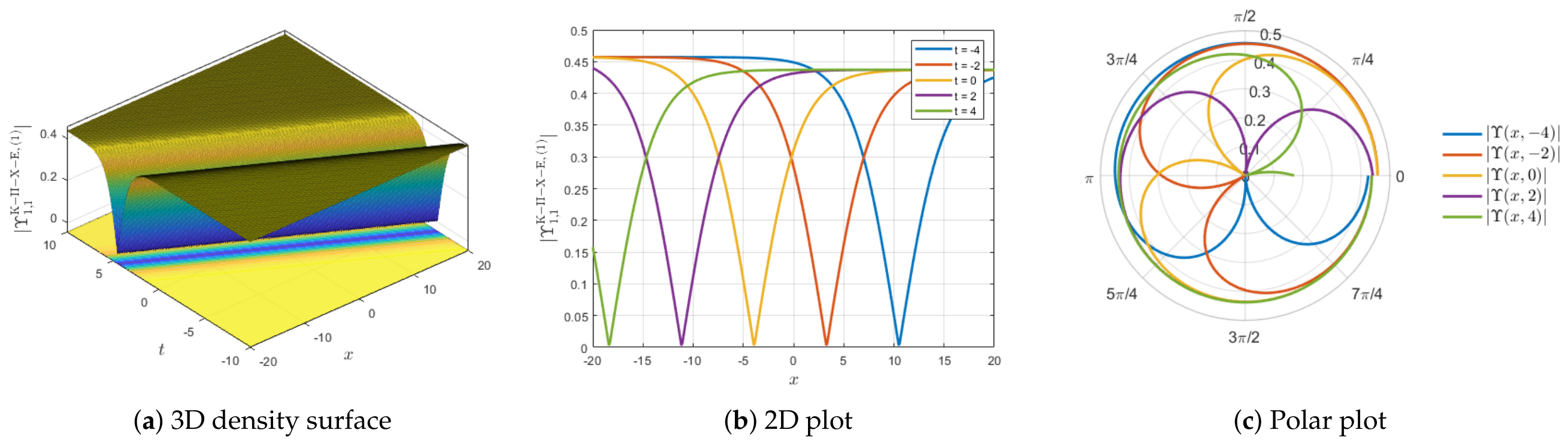
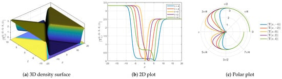
Figure 4 illustrates the dynamical profile of the dark soliton solution (9) for $\breve{\kappa }=-0.8$, $w_{x3}=0.25$, $w_{t3}=0.9$, $w_{y3}=0.02$, $b=0.01$, ${\breve{S}}_1=1.2$, and ${\breve{S}}_2=1.7$. The solution exhibits a localized intensity depression propagating on a continuous background, which is a characteristic feature of dark soliton structures. The three-dimensional density surface demonstrates stable localization and smooth propagation behavior, while the corresponding two-dimensional profile confirms the persistence of the amplitude dip without distortion. The polar plot further highlights the symmetric propagation dynamics and the stable wave configuration throughout the evolution process.

Figure 4. Dynamical profile of the dark soliton solution (9) with parameters $\breve{\kappa }=-0.8,$$w_{x3}=0.25,$$w_{t3}=0.9, w_{y3}=0.02, b=0.01, {\breve{S}}_1=1.2$, and ${\breve{S}}_2=1.7$.

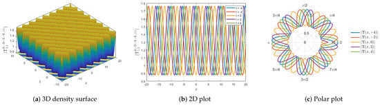
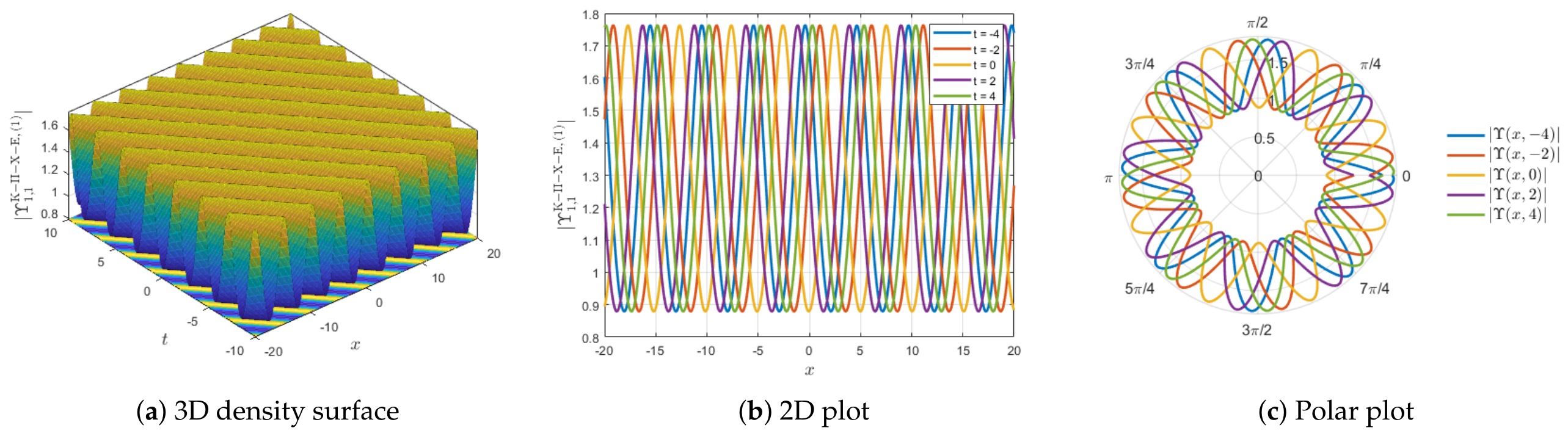
Figure 5 presents the periodic soliton solution (9) obtained for $\breve{\kappa }=1.55$, $w_{x3}=0.5$, $w_{t3}=0.9$, $w_{y3}=0.02$, $b=0.01$, ${\breve{S}}_1=1.2$, and ${\breve{S}}_2=1.7$. The solution displays pronounced oscillatory behavior with periodically repeating wave structures, indicating sustained nonlinear modulation. The three-dimensional density surface clearly captures the periodic evolution of the wave amplitudes, whereas the two-dimensional plot reveals regular oscillations with bounded amplitude. The polar representation confirms the cyclic propagation pattern and reflects the persistence of periodicity under the selected parameter regime.

Figure 5. Dynamical profile of the periodic soliton solution (9) with parameters $\breve{\kappa }=1.55,$$w_{x3}=0.5,$$w_{t3}=0.9, w_{y3}=0.02, b=0.01, {\breve{S}}_1=1.2$, and ${\breve{S}}_2=1.7$.

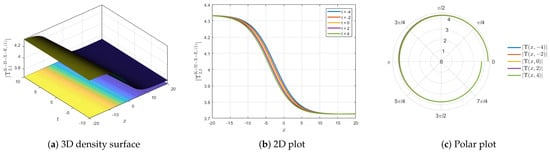
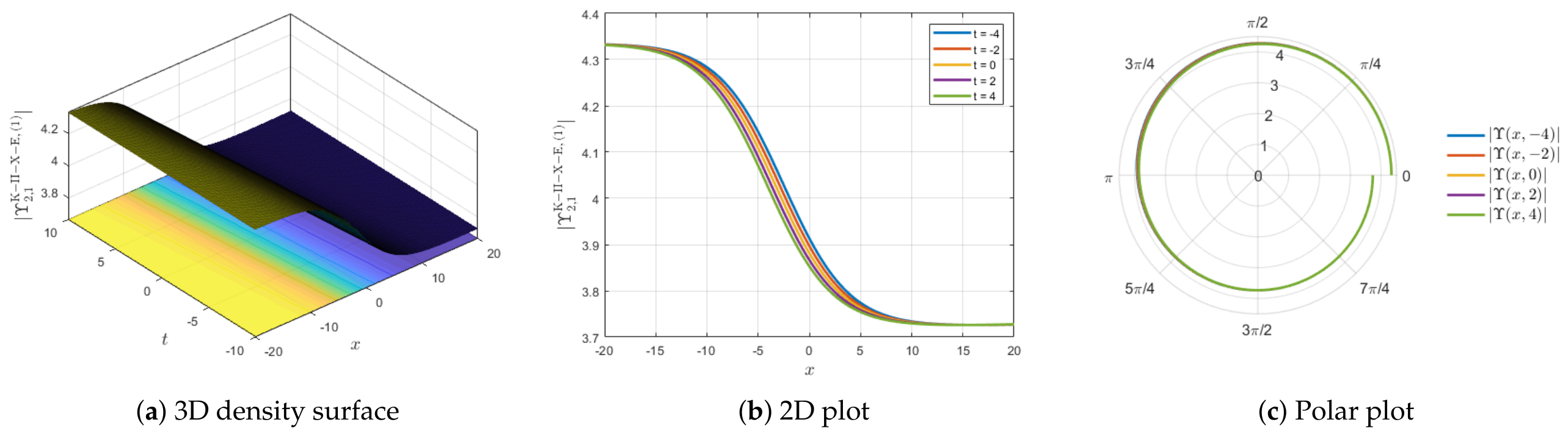
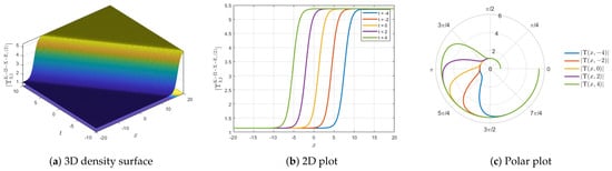
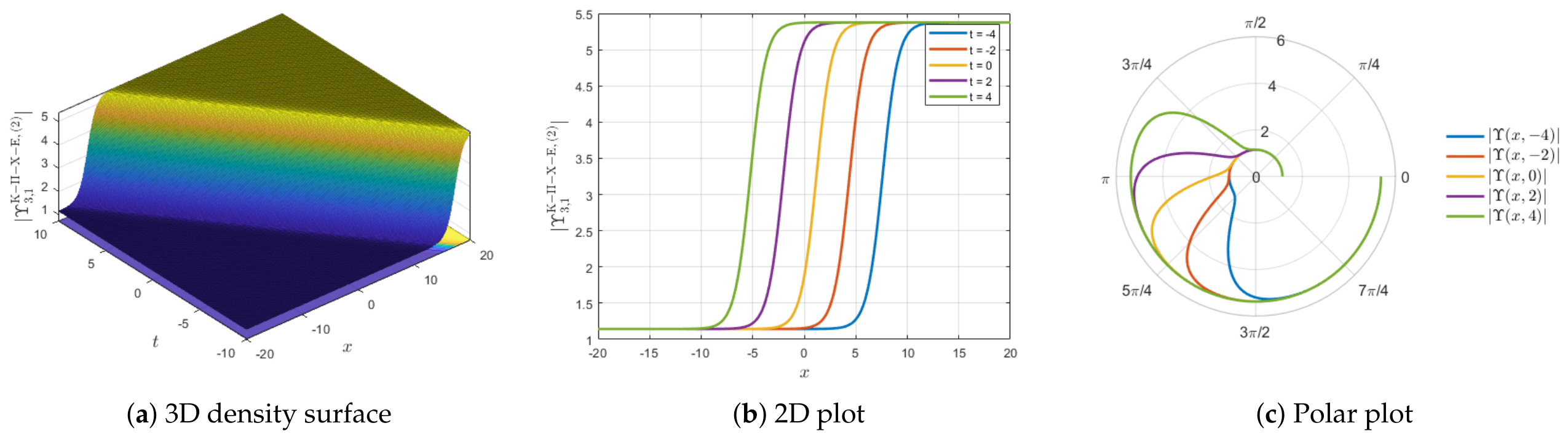
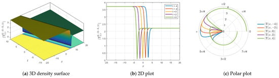
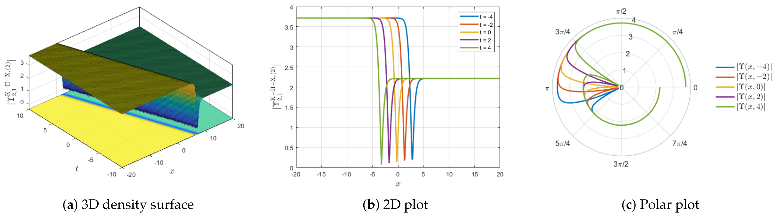
Figure 6 depicts the kink-type soliton solution (13) for $\breve{\kappa }=-0.004$, $\mu =1.20$, $w_{x3}=2.45$, $w_{t3}=0.495$, $w_{y3}=0.552$, $w_{24}=0.025$, $w_{34}=0.650$, $b=4.0$, ${\breve{S}}_1=0.75$, and ${\breve{S}}_2=1.9$. The obtained solution exhibits a smooth monotonic transition between two distinct asymptotic states, which is typical of kink wave structures. The density surface demonstrates stable propagation with strong localization, while the two-dimensional profile confirms the persistence of the kink front during evolution. The polar plot emphasizes the directional propagation and the robustness of the wave profile against deformation.

Figure 6. Dynamical profile of the kink type soliton solution (13) with parameters $\breve{\kappa }=-0.004,$$\mu =1.20,$$w_{x3}=2.45, w_{t3}=0.495, w_{y3}=0.552, w_{24}=0.025, w_{34}=0.650, b=4.0, {\breve{S}}_1=0.75,$${\breve{S}}_2=1.9$.

Figure 7 shows the dynamical behavior of the two-kink soliton solution (22) corresponding to $\breve{\kappa }=0.5$, $\breve{\lambda }=3.0$, $w_{x1}=0.6$, $w_{x2}=0.5$, $w_{t2}=0.8$, $w_{y1}=0.3$, $w_{y2}=0.2$, $b_1=0.1$, ${\breve{S}}_1=1.0$, and ${\breve{\mathcal{S}}}_2=0.5$. The solution demonstrates the coexistence and interaction of two distinct kink structures propagating simultaneously in the nonlinear medium. The three-dimensional density surface captures the interaction dynamics and stable propagation of both wave fronts, whereas the two-dimensional plot illustrates the preservation of their amplitudes and shapes during propagation. The polar plot further reveals the symmetric interaction characteristics and the coherent nature of the coupled kink structures.

Figure 7. Dynamical profile of the two-kink soliton solution (22) with parameters $\breve{\kappa }=0.5,$$\breve{\lambda }=3.0,$$w_{x1}=0.6, w_{x2}=0.5, w_{t2}=0.8, w_{y1}=0.3, w_{y2}=0.2, b_1=0.1, {\breve{S}}_1=1.0$, and ${\breve{\mathcal{S}}}_2=0.5$.

Figure 8 illustrates the dark-kink soliton solution (32) for $\breve{\kappa }=1.0$, $\breve{\lambda }=5.0$, $w_{t2}=0.8$, $w_{x2}=1.05$, $w_{y1}=0.05$, $w_{y2}=0.3$, $w_{1\mathrm{{\rm Y}}}=0.001$, $w_{2\mathrm{{\rm Y}}}=2.0$, $b_1=4.10$, ${\breve{S}}_1=1.0$, and ${\breve{\mathcal{S}}}_2=0.1$. The solution combines a localized dark structure with a kink-type transition, producing a hybrid nonlinear wave profile. The density surface demonstrates a stable localized depression coupled with a monotonic wave front, while the two-dimensional plot highlights the coexistence of dark and kink characteristics within the same structure. The polar representation further confirms the stable propagation and nonlinear coupling behavior of the composite soliton wave.

Figure 8. Dynamical profile of the dark-kink soliton solution (32) with parameters $\breve{\kappa }=1.0,$$\breve{\lambda }=5.0,$$w_{t2}=0.8, w_{x2}=1.05, w_{y1}=0.05, w_{y2}=0.3, w_{1\mathrm{{\rm Y}}}=0.001, w_{2\mathrm{{\rm Y}}}=2.0, b_1=4.10, {\breve{S}}_1=1.0$, and ${\breve{\mathcal{S}}}_2=0.1$.

Figure 9 presents the kink soliton solution (32) for $\breve{\kappa }=0.5$, $\breve{\lambda }=3.0$, $w_{t2}=0.8$, $w_{x2}=0.5$, $w_{y1}=0.3$, $w_{y2}=0.2$, $w_{1\mathrm{{\rm Y}}}=1.2$, $w_{2\mathrm{{\rm Y}}}=0.8$, $b_1=0.1$, ${\breve{S}}_1=1.0$, and ${\breve{\mathcal{S}}}_2=0.5$. The solution exhibits a smooth and stable kink profile characterized by a continuous transition between two equilibrium states. The three-dimensional density surface confirms the persistence of the localized wave front, whereas the two-dimensional plot demonstrates stable amplitude propagation without distortion. The polar plot further reflects the coherent directional propagation and the robustness of the nonlinear structure under the selected parameters.

Figure 9. Dynamical profile of the kink soliton solution (32) with parameters $\breve{\kappa }=0.5, \breve{\lambda }=3.0,$$w_{t2}=0.8,$$w_{x2}=0.5, w_{y1}=0.3, w_{y2}=0.2, w_{1\mathrm{{\rm Y}}}=1.2, w_{2\mathrm{{\rm Y}}}=0.8, b_1=0.1, {\breve{S}}_1=1.0$, and ${\breve{\mathcal{S}}}_2=0.5$.

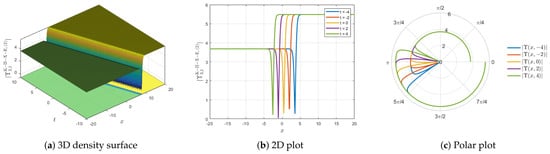
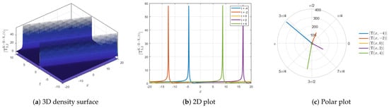
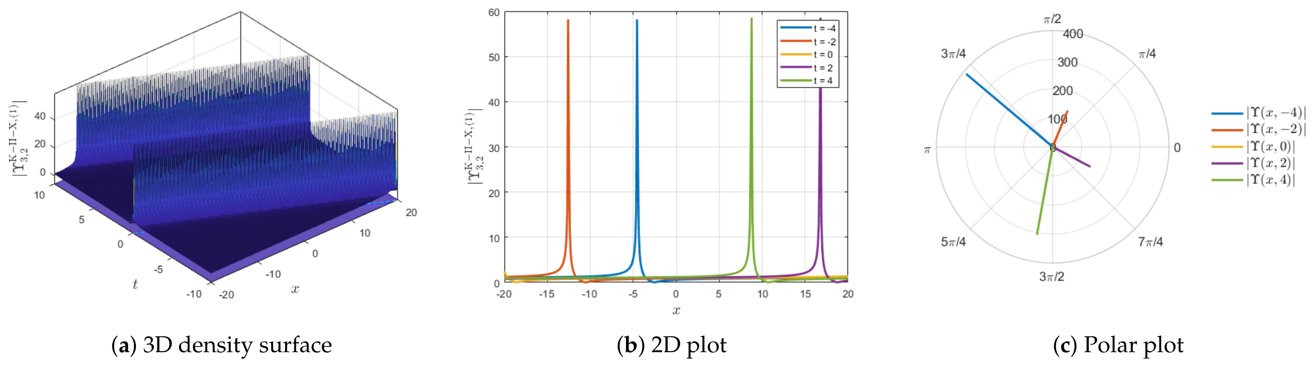
Figure 10 depicts the singular soliton solution (48) for $\kappa =3.0$, $w_{x3}=0.02$, $w_{t3}=0.08$, $w_{y3}=0.002$, $b=1.0$, ${\breve{S}}_1=1.50$, and ${\breve{\mathcal{S}}}_2=1.75$. The solution is characterized by sharp amplitude peaks and highly localized singular behavior, indicating the emergence of extreme nonlinear wave structures. The three-dimensional density surface clearly illustrates steep gradients and strong localization, while the two-dimensional profile emphasizes the singular amplitude growth. The polar plot further captures the directional concentration of the singularity and reflects the highly localized propagation dynamics.

Figure 10. Dynamical profile of the singular soliton solution (48) with parameters $\kappa =3.0, w_{x3}=0.02,$$w_{t3}=0.08, w_{y3}=0.002, b=1.0, {\breve{S}}_1=1.50$, and ${\breve{\mathcal{S}}}_2=1.75$.

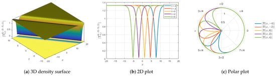
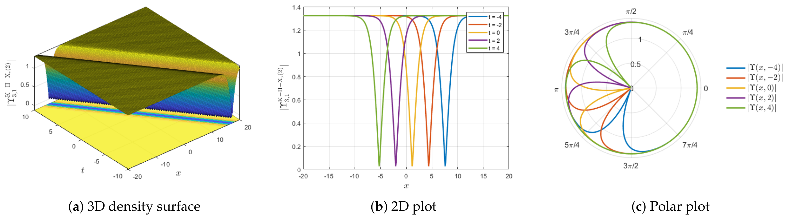
Figure 11 presents the dark-kink soliton solution (57) corresponding to $\breve{\kappa }=0.12$, $\breve{\lambda }=3.06$, $w_{t1}=0.75$, $w_{x1}=0.995$, $w_{y1}=0.03$, $w_{y2}=0.02$, $w_{2\mathrm{{\rm Y}}}=1.8$, $b_1=0.01$, ${\breve{S}}_1=1.0$, and ${\breve{\mathcal{S}}}_2=0.5$. The obtained structure demonstrates the coexistence of a localized dark intensity dip together with a kink-type transition profile. The density surface illustrates stable propagation and strong nonlinear localization, whereas the two-dimensional plot confirms the persistence of the combined wave structure without noticeable deformation. The polar representation further highlights the hybrid propagation characteristics and the coherent interaction between the dark and kink components.

Figure 11. Dynamical profile of the dark kink soliton solution (57) with parameters $\breve{\kappa }=0.12,$$\breve{\lambda }=3.06,$$w_{t1}=0.75, w_{x1}=0.995, w_{y1}=0.03, w_{y2}=0.02, w_{2\mathrm{{\rm Y}}}=1.8, b_1=0.01, {\breve{S}}_1=1.0$, and ${\breve{\mathcal{S}}}_2=0.5$.

Finally, Figure 12 illustrates the dark soliton solution (61) for $\breve{\kappa }=0.5$, $\breve{\lambda }=3.0$, $w_{t2}=0.8$, $w_{x2}=0.5$, $w_{y2}=0.2$, $b_1=1.5$, ${\breve{S}}_1=1.0$, and ${\breve{\mathcal{S}}}_2=0.5$. The solution exhibits a stable localized intensity depression propagating on a finite continuous background. The three-dimensional density surface confirms strong localization and smooth wave evolution, while the two-dimensional profile demonstrates the preservation of the dark amplitude notch during propagation. The polar plot further reveals the symmetric propagation characteristics and stability of the nonlinear dark soliton structure.

Figure 12. Dynamical profile of the dark soliton solution (61) with parameters $\breve{\kappa }=0.5, \breve{\lambda }=3.0,$$w_{t2}=0.8,$$w_{x2}=0.5, w_{y2}=0.2, b_1=1.5, {\breve{S}}_1=1.0$, and ${\breve{\mathcal{S}}}_2=0.5$.

Importance of the Solutions

The $(2+1)$-dimensional K-II-X-E- and K-II-X-type equations have a rich variety of nonlinear wave structures in various parametric regimes, each of which has a different physical meaning. These solutions demonstrate the capability of the considered models to describe diverse localized and nonlocalized wave structures that are fundamentally important in nonlinear science, mathematical physics, plasma dynamics, optical communication systems, fluid mechanics, and dispersive media.

The dark soliton solutions obtained in the present study represent localized intensity depressions propagating on a continuous-wave background while preserving their shape and stability during evolution. Such structures play a significant role in defocusing nonlinear media, nonlinear optical fibers, Bose–Einstein condensates, and hydrodynamic systems, where stable energy redistribution and phase-modulated propagation are essential. The associated three-dimensional density surfaces, two-dimensional profiles, and polar representations confirm the persistence and robustness of these localized dark structures under different parameter choices. The periodic soliton solutions illustrate the existence of bounded oscillatory wave patterns with repeating nonlinear modulation. These solutions are physically important for modeling recurrent wave propagation, modulation instability, nonlinear pattern formation, and energy transport phenomena in dispersive environments. Their oscillatory characteristics indicate the ability of the governing equations to sustain stable periodic wave trains over long propagation intervals without significant distortion. The kink-type soliton solutions correspond to smooth monotonic transitions between two distinct asymptotic states and are closely related to nonlinear front propagation, domain-wall dynamics, and switching mechanisms in physical systems. Such solutions arise naturally in plasma physics, nonlinear transmission lines, fluid interfaces, and quantum field models. The observed stability and localization properties of these kink structures confirm the effectiveness of the models in describing nonlinear transition phenomena and propagating wave fronts in higher-dimensional media. The obtained two-kink soliton solutions further demonstrate the coexistence and simultaneous propagation of multiple nonlinear transition waves within the same medium. These structures provide important insight into coupled nonlinear excitations and coherent wave interactions occurring in complex dispersive systems. The preservation of the wave profiles during propagation indicates the stability and robustness of the interacting kink structures. In addition, the dark-kink soliton solutions reveal hybrid nonlinear behaviors formed through the interaction of localized dark intensity depressions with monotonic kink-type wave fronts. These composite structures are particularly important in describing coupled energy-transfer mechanisms, nonlinear interface dynamics, and mixed propagation states in optical and plasma systems. The coexistence of dark and kink characteristics reflects the rich nonlinear superposition properties supported by the considered equations. The singular soliton solutions exhibit sharply localized amplitude peaks and steep nonlinear gradients, representing extreme wave localization and threshold-driven nonlinear behavior. Such singular structures are closely connected with rogue-wave precursors, nonlinear focusing effects, and highly concentrated energy states appearing in plasma systems, fluid dynamics, and optical pulse propagation. The strong localization observed in the density surfaces and two-dimensional profiles demonstrates the capability of the models to capture highly nonlinear and potentially unstable physical processes.

Moreover, the obtained solutions emphasize the importance of multidimensional nonlinear interactions and demonstrate the capability of the governing equations to describe stable propagation, oscillatory dynamics, localized energy transport, nonlinear coupling, and wave interaction phenomena simultaneously. The corresponding polar plots reveal additional information regarding directional propagation, rotational symmetry, and coherent wave evolution, thereby providing deeper insight into the geometric behavior of the obtained solutions.

Therefore, the diversity, stability, and physical richness of the derived soliton structures confirm the effectiveness of the proposed K-II-X-E- and K-II-X-type models in describing complex nonlinear wave propagation in higher-dimensional dispersive systems. The robustness of the obtained solutions under varying parameter regimes further highlights their applicability in the mathematical modeling of realistic physical phenomena involving nonlinear localization, energy exchange, wave modulation, and coherent interaction dynamics. Consequently, the present results contribute significantly to the theoretical understanding of nonlinear evolution equations and their applications in modern mathematical physics and applied nonlinear sciences.

5. Conclusions

This study presents an NN-based $(G^{\prime }/G)$-expansion method to obtain exact analytical soliton solutions of the integrable $(2+1)$-dimensional K-II-X-E- and K-II-X-type models. The main contribution of this work lies in employing the $(G^{\prime }/G)$-expansion function as an interpretable activation mechanism within an NN framework. In this formulation, the solution structure of the Riccati equation is embedded into the first layer of the network, enabling the generation of analytically consistent extended trial functions through forward propagation. This mechanism establishes a direct and systematic connection between classical analytical techniques and symbolic NN representations, providing a transparent and reliable framework for the construction of exact solutions. Using the proposed approach, several types of soliton solutions were obtained in trigonometric, hyperbolic, and rational forms. These solutions correspond to several important nonlinear wave structures, including dark solitons, periodic solitons, kink solitons, two-kink solitons, dark-kink solitons, and singular soliton waves, each exhibiting distinct localization, oscillatory, and interaction characteristics in higher-dimensional nonlinear dispersive media. The solutions satisfy the governing equations exactly and exhibit stable behavior over long propagation distances, thus proving their mathematical correctness and physical relevance. In order to obtain a better understanding of the behavior of the solution, detailed plots in 2D and 3D surface graphs and polar representations were presented. These visual tools make the wave dynamics much easier to interpret and give a clear insight on the non-linear features of the K-II-X-E- and K-II-X-type models.

The proposed approach of $(G^{\prime }/G)$-ENNs framework is a powerful and versatile tool for solving NPDEs. Future studies may look into the K-II type of equations with variable coefficients or fractional order operators to obtain spatial variation as well as memory effects. The stability of obtained soliton solutions like modulation instability and response to perturbations can also be investigated. Moreover, more advanced neural network methods such as PINNs can potentially be used to study higher dimensions nonlinear equations and coupled systems and provide an effective framework to analyze more complicated wave phenomena in applications to physical and engineering sciences.

References

- Akinyemi, L.; Houwe, A.; Abbagari, S.; Wazwaz, A.M.; Alshehri, H.M.; Osman, M.S. Effects of the higher-order dispersion on solitary waves and modulation instability in a monomode fiber. Optik 2023, 288, 171202. [Google Scholar] [CrossRef] [Scilit]
- Zhou, Y. Lump and rogue wave solutions to (1 + 1)-dimensional evolution equations. Partial. Differ. Equ. Appl. Math. 2022, 5, 100252. [Google Scholar] [CrossRef] [Scilit]
- Ismael, H.F.; Sulaiman, T.A.; Nabi, H.R.; Mahmoud, W.; Osman, M.S. Geometrical patterns of time variable Kadomtsev–Petviashvili (I) equation that models dynamics of waves in thin films with high surface tension. Nonlinear Dyn. 2023, 111, 9457–9466. [Google Scholar] [CrossRef] [Scilit]
- Younas, U.; Seadawy, A.R.; Younis, M.; Rizvi, S.T.; Althobaiti, S. Diverse wave propagation in shallow water waves with Kadomtsev–Petviashvili–Benjamin–Bona–Mahony and Benney–Luke integrable models. Open Phys. 2021, 19, 808–818. [Google Scholar] [CrossRef] [Scilit]
- Li, Q.; Shan, W.; Wang, P.; Cui, H. Breather, lump and N-soliton wave solutions of the (2 + 1)-dimensional coupled nonlinear partial differential equation with variable coefficients. Commun. Nonlinear Sci. Numer. Simul. 2022, 106, 106098. [Google Scholar] [CrossRef] [Scilit]
- Tripathy, A.; Sahoo, S.; Rezazadeh, H.; Izgi, Z.P.; Osman, M.S. Dynamics of damped and undamped wave natures in ferromagnetic materials. Optik 2023, 281, 170817. [Google Scholar] [CrossRef] [Scilit]
- Khater, M.M.A. Non-linear biological population model; computational and numerical investigations. Chaos Solitons Fractals 2022, 162, 112388. [Google Scholar] [CrossRef] [Scilit]
- Horikis, T.P.; Frantzeskakis, D.J.; Smyth, N.F. Extended shallow water wave equations. Wave Motion 2022, 112, 102934. [Google Scholar] [CrossRef] [Scilit]
- Kudryashov, N.A. On ’new travelling wave solutions’ of the KdV and the KdV-Burgers equations. Commun. Nonlinear Sci. Numer. Simul. 2009, 14, 1891–1900. [Google Scholar] [CrossRef] [Scilit]
- Wang, M.; Li, X.; Zhang, J. The (G′/G)-expansion method and travelling wave solutions of nonlinear evolution equations in mathematical physics. Phys. Lett. A 2008, 372, 417–423. [Google Scholar] [CrossRef] [Scilit]
- Burcu, A.; Ahmet, B. The (G′/G)-expansion method for the nonlinear lattice equations. Commun. Nonlinear Sci. Numer. Simul. 2012, 17, 3490–3498. [Google Scholar] [CrossRef] [Scilit]
- Baber, M.Z.; Seadawy, A.R.; Qasim, M.; Iqbal, M.S.; Rizvi, S.T. On the spatiotemporal structures of ratio-dependent prey–predator model of ecological system. Int. Geom. Methods Mod. Phys. 2024, 21, 2450079. [Google Scholar] [CrossRef] [Scilit]
- Malik, S.; Hashemi, M.S.; Kumar, S.; Rezazadeh, H.; Mahmoud, W.; Osman, M.S. Application of new Kudryashov method to various nonlinear partial differential equations. Opt. Quantum Electron. 2023, 55, 8. [Google Scholar]
- Inc, M.; Iqbal, M.S.; Baber, M.Z.; Qasim, M.; Iqbal, Z.; Tarar, M.A.; Ali, A.H. Exploring the solitary wave solutions of Einstein’s vacuum field equation in the context of ambitious experiments and space missions. Alex. Eng. J. 2023, 82, 186–194. [Google Scholar] [CrossRef] [Scilit]
- Iqbal, M.S.; Seadawy, A.R.; Baber, M.Z.; Qasim, M. Application of modified exponential rational function method to Jaulent–Miodek system leading to exact classical solutions. Chaos Solitons Fractals 2022, 164, 112600. [Google Scholar] [CrossRef] [Scilit]
- Zafar, A.; Shakeel, M.; Ali, A.; Akinyemi, L.; Rezazadeh, H. Optical solitons of nonlinear complex Ginzburg–Landau equation via two modified expansion schemes. Opt. Quantum Electron. 2022, 54, 5. [Google Scholar]
- Zhang, J.L.; Wang, M.L.; Wang, Y.M.; Fang, Z.D. The improved F-expansion method and its applications. Phys. Lett. A 2006, 350, 103–109. [Google Scholar] [CrossRef] [Scilit]
- Akinyemi, L.; Şenol, M.; Osman, M.S. Analytical and approximate solutions of nonlinear Schrödinger equation with higher dimension in the anomalous dispersion regime. J. Ocean. Eng. Sci. 2022, 7, 143–154. [Google Scholar] [CrossRef] [Scilit]
- Rehman, H.U.; Akber, R.; Wazwaz, A.M.; Alshehri, H.M.; Osman, M.S. Analysis of Brownian motion in stochastic Schrödinger wave equation using Sardar sub-equation method. Optik 2023, 289, 171305. [Google Scholar] [CrossRef] [Scilit]
- Singh, S.; Ray, S.S. New analytical solutions and integrability for the (2 + 1)-dimensional variable coefficients generalized Nizhnik-Novikov-Veselov system arising in the study of fluid dynamics via auto-Backlund transformation approach. Phys. Scr. 2023, 98, 085243. [Google Scholar] [CrossRef] [Scilit]
- Qasim, M.; Yao, F.; Baber, M.Z.; Younas, U. Investigating the higher dimensional Kadomtsev–Petviashvili–Sawada–Kotera–Ramani equation: Exploring the modulation instability, Jacobi elliptic and soliton solutions. Phys. Scr. 2025, 100, 025215. [Google Scholar] [CrossRef] [Scilit]
- Wazwaz, A.M. A sine–cosine method for handling nonlinear wave equations. Math. Comput. Model. 2004, 40, 499–503. [Google Scholar] [CrossRef] [Scilit]
- Sağlam, F.N.K.; Malik, S. Various traveling wave solutions for (2 + 1)-dimensional extended Kadomtsev–Petviashvili equation using a newly created methodology. Chaos Solitons Fractals 2024, 186, 115318. [Google Scholar] [CrossRef] [Scilit]
- Akram, G.; Arshed, S.; Sadaf, M.; Khan, A. Extraction of new soliton solutions of (3+1)-dimensional nonlinear extended quantum Zakharov-Kuznetsov equation via generalized exponential rational function method and (G′/G, 1/G)-expansion method. Opt. Quantum Electron. 2024, 56, 829. [Google Scholar] [CrossRef] [Scilit]
- Roshid, M.M.; Uddin, M.; Boulaaras, S.; Osman, M.S. Dynamic optical soliton solutions of M-fractional modify unstable nonlinear Schrödinger equation via two analytic methods. Results Eng. 2025, 25, 103757. [Google Scholar] [CrossRef] [Scilit]
- Sasaki, H. On inverse scattering for the two-dimensional nonlinear Schrödinger equation. J. Differ. Equ. 2024, 401, 308–333. [Google Scholar] [CrossRef] [Scilit]
- Khalil, T.A.; Ahmed, H.M.; Ahmed, K.K.; Emadifar, H.; Rabie, W.B. Innovative optical solitons and other exact wave solutions for coupled system of new nonlocal LPDE using improved modified extended tanh technique. Results Opt. 2025, 21, 100853. [Google Scholar] [CrossRef] [Scilit]
- Hirota, R. The Direct Method in Soliton Theory; Cambridge University Press: Cambridge, UK, 2004. [Google Scholar]
- Zhang, R.F.; Li, M.C.; Gan, J.Y.; Li, Q.; Lan, Z.Z. Novel trial functions and rogue waves of generalized breaking soliton equation via bilinear neural network method. Chaos Solitons Fractals 2022, 154, 111692. [Google Scholar] [CrossRef] [Scilit]
- Li, S.A.; Cao, J.D.; Liu, H.; Huang, C.D. Delay-dependent parameters bifurcation in a fractional neural network via geometric methods. Appl. Math. Comput. 2024, 478, 128812. [Google Scholar] [CrossRef] [Scilit]
- Wang, S.P.; Zhang, H.; Jiang, X.Y. Physics-informed neural network algorithm for solving forward and inverse problems of variable-order space-fractional advection-diffusion equations. IEEE/CAA J. Autom. Sin. 2023, 535, 64–82. [Google Scholar] [CrossRef] [Scilit]
- LeCun, Y.; Bengio, Y.; Hinton, G. Deep Learning. Nature 2015, 521, 436–444. [Google Scholar] [CrossRef] [Scilit] [PubMed]
- Krizhevsky, A.; Sutskever, I.; Hinton, G.E. Imagenet classification with deep convolutional neural networks. Adv. Neural Inf. Process. Syst. 2012, 25, 1–9. [Google Scholar]
- Voulodimos, A.; Doulamis, N.; Doulamis, A.; Protopapadakis, E. Deep Learning for Computer Vision: A Brief review. Comput. Intell. Neurosci. 2018, 2018, 7068349. [Google Scholar] [CrossRef] [Scilit] [PubMed]
- Hirschberg, J.; Manning, C.D. Advances in natural language processing. Science 2015, 349, 261–266. [Google Scholar] [CrossRef] [Scilit]
- Sekban, D.M.; Yaylacı, E.U.; Özdemir, M.E.; Yaylacı, M.; Tounsi, A. Investigating formability behavior of friction stir-welded high-strength shipbuilding steel using experimental, finite element, and artificial neural network methods. J. Mater. Eng. Perform. 2025, 34, 4942–4950. [Google Scholar]
- Liu, Y.; Yuan, S.; Zhang, R.; Yan, L.; Dong, H.; Feng, L. A novel (G′/G)-expansion neural network method for exact analytical solutions of nonlinear partial differential equations. Nonlinear Dyn. 2025, 113, 26603–26630. [Google Scholar] [CrossRef] [Scilit]
- Dissanayake, M.G.; Phan-Thien, N. Neural-network-based approximations for solving partial differential equations. Commun. Numer. Methods Eng. 1994, 10, 195–201. [Google Scholar] [CrossRef] [Scilit]
- Liu, Y.Q.; Mao, T.; Zhou, D.X. Approximation of functions from Korobov spaces by shallow neural networks. Inf. Sci. 2024, 670, 120573. [Google Scholar] [CrossRef] [Scilit]
- Principe, J.C.; Chen, B.D. Universal approximation with convex optimization: Gimmick or reality? IEEE Comput. Intell. Mag. 2015, 10, 68–77. [Google Scholar] [CrossRef] [Scilit]
- Zhang, Z.Z.; Bao, F.; Ju, L.L.; Zhang, G.N. Transferable neural networks for partial differential equations. J. Sci. Comput. 2024, 99, 2. [Google Scholar] [CrossRef] [Scilit]
- Liu, X.H.; Li, Y.F.; Xu, G.J. Finite-time synchronization analysis for the generalized Caputo fractional spatio-temporal neural networks. Math. Comput. Simul. 2025, 230, 94–110. [Google Scholar] [CrossRef] [Scilit]
- Raissi, M.; Perdikaris, P.; Karniadakis, G.E. Physics-informed neural networks: A deep learning framework for solving forward and inverse problems involving nonlinear partial differential equations. J. Comput. Phys. 2019, 378, 686–707. [Google Scholar] [CrossRef] [Scilit]
- Pang, G.F.; Lu, L.; Karniadakis, G.E. fPINNs: Fractional physics-informed neural networks. Siam J. Sci. Comput. 2019, 41, A2603–A2626. [Google Scholar] [CrossRef] [Scilit]
- Tipu, G.H.; Cherati, A.Y.; Yao, F.; Momeni, H. Data-driven soliton solutions and parameter discovery to the fourth-order nonlinear AKNS equation: A hybrid analytical and physics-informed neural network approach. Nonlinear Dyn. 2025, 113, 25047–25069. [Google Scholar] [CrossRef] [Scilit]
- Pu, J.; Chen, Y. Darboux transformation-based LPNN generating novel localized wave solutions. Phys. D Nonlinear Phenom. 2024, 467, 134262. [Google Scholar] [CrossRef] [Scilit]
- Akram, S.; Rahman, M.U.; Al-Essa, L.A. Inelastic lump–breather interactions and periodic wave dynamics in the generalized Calogero–Bogoyavlenskii–Schiff equation via a bilinear neural architecture. Eur. Phys. J. Spec. Top. 2026, 1–20. [Google Scholar] [CrossRef] [Scilit]
- Hai, N.; Bilige, S. Using the bilinear neural network method and the neural network-based symbolic calculation approach to find exact solutions of the (3 + 1)-dimensional Kairat-X extended equation. Nonlinear Dyn. 2025, 113, 27941–27960. [Google Scholar] [CrossRef] [Scilit]
- Tipu, G.H.; Mateen, A.; Davletov, E.; Davletov, I.; Javed, F. Novel soliton dynamics via (G′/G)-expansion neural networks approach in the modified Camassa–Holm and Kuramoto–Sivashinsky models. Mod. Phys. Lett. B 2026, 2650036. [Google Scholar] [CrossRef] [Scilit]
- Isah, M.A.; Yokus, A.; Kaya, D. Exploring the influence of layer and neuron configurations on Boussinesq equation solutions via a bilinear neural network framework. Nonlinear Dyn. 2024, 112, 13361–13377. [Google Scholar] [CrossRef] [Scilit]
- Wu, F.; Raihen, M.N.; Baskonus, H. M On the exploring of the new complex and mixed hyperbolic properties of the nonlinear Kairat-II-X models. Nonlinear Dyn. 2025, 113, 20385–20406. [Google Scholar] [CrossRef] [Scilit]
- Faridi, W.A.; Wazwaz, A.M.; Mostafa, A.M.; Myrzakulov, R.; Umurzakhova, Z. The Lie point symmetry criteria and formation of exact analytical solutions for Kairat-II equation: Paul-Painlevé approach. Chaos Solitons Fractals 2024, 182, 114745. [Google Scholar] [CrossRef] [Scilit]
- Awadalla, M.; Zafar, A.; Taishiyeva, A.; Raheel, M.; Myrzakulov, R.; Bekir, A. Exact soliton solutions of M-fractional Kairat-II and Kairat-X equations via three analytical methods. Front. Phys. 2024. [Google Scholar] [CrossRef]
- Demirbilek, U.; Tedjani, A.H.; Seadawy, A.R. Analytical solutions of the combined Kairat-II-X equation: A dynamical perspective on bifurcation, chaos, energy, and sensitivity. Aims Math. 2025, 10, 13664–13691. [Google Scholar] [CrossRef] [Scilit]
- Wazwaz, A.M. Extended (3 + 1)-dimensional Kairat-II and Kairat-X equations: Painlevé integrability, multiple soliton solutions, lump solutions, and breather wave solutions. Int. J. Numer. Methods Heat Fluid Flow 2024, 34, 2177–2194. [Google Scholar] [CrossRef] [Scilit]
- Mehanna, M.; Wazwaz, A.M. Tri-analytical approach to Kairat-II and Kairat-X equations. Rom. Rep. Phys. 2025, 77, 107. [Google Scholar] [CrossRef] [Scilit]
- Mateen, A.; Tipu, G.H.; Ciurdariu, L.; Yao, F. Analytical soliton solutions of the Kairat-II equation using the Kumar–Malik and extended hyperbolic function methods. Aims Math. 2025, 10, 8721–8752. [Google Scholar] [CrossRef] [Scilit]
- Alhakim, L.; Gasmi, B.; Moussa, A.; Mati, Y. Bifurcation, chaotic behavior, and soliton solutions of the Kairat-II equation via two analytical methods. Partial. Differ. Equ. Appl. Math. 2025, 13, 101135. [Google Scholar] [CrossRef] [Scilit]
- Awadalla, M.; Zafar, A.; Taishiyeva, A.; Raheel, M.; Myrzakulov, R.; Bekir, A. The analytical solutions to the M-fractional Kairat-II and Kairat-X equations. Front. Phys. 2023, 11, 1335423. [Google Scholar]
- Wazwaz, A.M. Exploring multiple soliton solutions and lump wave solutions to two integrable (2 + 1)-dimensional Kairat-II-X-extended and Kairat-II-X-type equations. Int. J. Numer. Methods Heat Fluid Flow 2025, 36, 145–164. [Google Scholar] [CrossRef] [Scilit]
Disclaimer/Publisher’s Note: The statements, opinions and data contained in all publications are solely those of the individual author(s) and contributor(s) and not of MDPI and/or the editor(s). MDPI and/or the editor(s) disclaim responsibility for any injury to people or property resulting from any ideas, methods, instructions or products referred to in the content. |
© 2026 by the authors. Licensee MDPI, Basel, Switzerland. This article is an open access article distributed under the terms and conditions of the Creative Commons Attribution (CC BY) license.