


Abstract
Safety alignment of large language models faces a feedback dilemma: human judgment is reliable but costly to scale; automated judgment is cheap but less trustworthy. Existing methods commit to one source per run, so misjudged responses are never corrected. This paper proposes Hybrid RLHF-AIF, which picks the feedback source for each sample online. First, a multi-label DistilBERT discriminator scores every response across 19 harm categories, reporting confidence through Monte Carlo dropout. Second, an uncertainty-aware scheduler sends only ambiguous or low-confidence responses to the reliable reviewer channel under a fixed budget and the rest to an artificial intelligence (AI) evaluator, recomputing the decision inside every Proximal Policy Optimization (PPO) iteration so that routing follows the policy. Collected annotations are replayed so the discriminator tracks the shifting policy. The reviewer channel is a stronger language model, not a real annotator, so the savings concern simulated human feedback. On PKU-SafeRLHF and HH-RLHF, over five seeds, the framework matches the safety of full simulated-human supervision on 10% of that budget while staying markedly more helpful and natural. Because that discriminator would otherwise judge its own objective, all final policies are re-scored with Llama Guard 3, and utility is re-judged by Claude Opus 5, a model from a different vendor; the ordering of methods survives both.
Keywords:
large language models; safety alignment; reinforcement learning from human feedback; reinforcement learning from AI feedback; simulated human feedback; uncertainty estimation; Monte Carlo dropout; proximal policy optimization; human-in-the-loop MSC:
68T50; 68T05; 68T37
1. Introduction
Large language models (LLMs), built on the transformer architecture [1] and scaled into systems such as GPT-4 [2] and the Llama family [3,4], are now deployed in open-ended interactive systems [5,6], and the same generative recipe has been carried beyond text into images, 3D content, animation, and other structured artifacts [7,8,9,10], widening the range of behavior that requires safety oversight. Controlling harmful outputs remains an open problem, because even rare unsafe responses carry legal, social, and ethical consequences [11,12,13], and aligning model behavior with human values has become a central research direction [14,15,16]. Those consequences are not spread evenly, which makes the problem a societal one and not only a technical one. Harm falls hardest on the groups a safety taxonomy represents least well, so an evaluator that is systematically weaker on some harm categories passes its blind spots to every model it supervises, a fairness failure as much as a safety failure [12,17]. Trustworthiness is squeezed from the other side: a model that manages risk by refusing broadly withholds legitimate help, and over-refusal is paid for by the users who most need an answer [18]. Cost decides who can avoid both failures, because when reliable oversight is expensive, only well-funded deployments can buy it and the rest fall back on the cheapest automated judgment available. The central difficulty is therefore economic as much as technical: reliable safety signals are costly, and cheap safety signals are unreliable.
Existing alignment methods resolve this tension by committing to one side of it. Reinforcement Learning from Human Feedback (RLHF) treats human judgments as the reward and produces dependable safety signals [19,20,21,22], yet human annotation is expensive and hard to scale. Reinforcement Learning from AI Feedback (RLAIF) replaces human annotators with model-generated evaluations and slashes cost [23,24], but it risks amplifying the biases of the evaluator model [25]. Targeted Human Feedback (RLTHF) begins to combine the two by correcting AI labels with selective human annotation [26], but its routing is fixed before training starts and cannot adapt as the policy changes. As a result, the samples on which the AI evaluator is least reliable go undetected once the policy distribution drifts away from the pre-training split.
This gap can be closed because an automated evaluator does not fail at random. Reward-model ensembles show that high reward uncertainty concentrates on a small fraction of samples and tracks overoptimization risk [27], and targeted-feedback work shows that correcting only the 6% to 7% of AI labels the labeler is most likely to get wrong recovers full-human alignment quality [26], which would be impossible if errors were spread uniformly. Both findings point to the same structure: evaluator errors cluster. Model uncertainty, which rises where a model lacks knowledge rather than where the data are merely noisy [28,29], offers a practical handle on that clustering. Tracked during training, it identifies the few samples on which the AI is unreliable and escalates them as they arise, instead of after training is over.
Turning this principle into a working system raises three challenges. First, a safety reward must capture risk along many dimensions at once, since a single scalar cannot express that a response is simultaneously hateful, violent, and self-harm related [14,17]. Second, the automated reward is itself uncertain, and if that uncertainty goes unmeasured, the policy can lock onto scores that are confident but wrong, the overoptimization failure documented for reward models [27,30,31]. Third, the reliable channel cannot cover every sample, so a fixed budget must go to the samples that need it most [20].
These three challenges shape the design of Hybrid RLHF-AIF, which rests on a single idea: let the evaluator’s own uncertainty decide, at each training step, which feedback source a sample needs, so that the reliable channel is spent only where the AI is unreliable. A multi-label safety discriminator, pretrained on PKU-SafeRLHF [32], outputs a 19-dimensional vector of risk probabilities for each response, separating harm types instead of collapsing them into one number. That vector drives the routing decision, not the reward: an uncertainty-aware scheduler estimates the discriminator’s confidence through Monte Carlo (MC) Dropout [28], sends low-confidence or risk-ambiguous responses to the reviewer channel and the rest to an AI evaluator, and the scalar reward that updates the policy comes from whichever source scored the sample. The two components form the loop in Figure 1: rollout, safety assessment, uncertainty-guided routing, PPO optimization. Because evaluator errors cluster on a small fraction of samples, a reviewer budget of 10% covers them in our setting, with margin for the added difficulty of multi-dimensional safety scoring. Section 4.5 sweeps this cap and places 10% at the knee of the utility curve rather than at an arbitrary point, but that knee is a property of this model, dataset, and evaluator triple, and we do not claim it as a general constant.
Figure 1.
Overview of the Hybrid RLHF-AIF framework, read as six steps. (1) Rollout: a prompt drawn from HH-RLHF is answered by the policy . (2) Safety assessment: the multi-label discriminator scores the response over 19 harm categories under Monte Carlo dropout passes, giving an aggregated risk score s (Equation (4)) and a predictive uncertainty u (Equation (7)). (3) Routing: the scheduler compares the pair against three thresholds, and bounding the ambiguous risk band and bounding acceptable uncertainty, and marks the sample for the reviewer channel when the risk is ambiguous () or the uncertainty is high (); Section 3.4 gives every case. (4) Feedback: (4a) a marked sample goes to the simulated human reviewer if the budget counter B is positive; a binary verdict is returned, and B is decremented; (4b) every other sample goes to the AI evaluator, which returns a continuous risk score . Roughly 10% and 90% of samples take the two paths. (5) Optimization: the resulting scalar reward drives the PPO update, whose internal mechanics are shown in Figure 2. (6) Adaptation: reviewer annotations are stored in a replay buffer that periodically fine-tunes , so the discriminator follows the policy distribution instead of the fixed pretraining one. The human channel is simulated by a language model throughout (Appendix C).
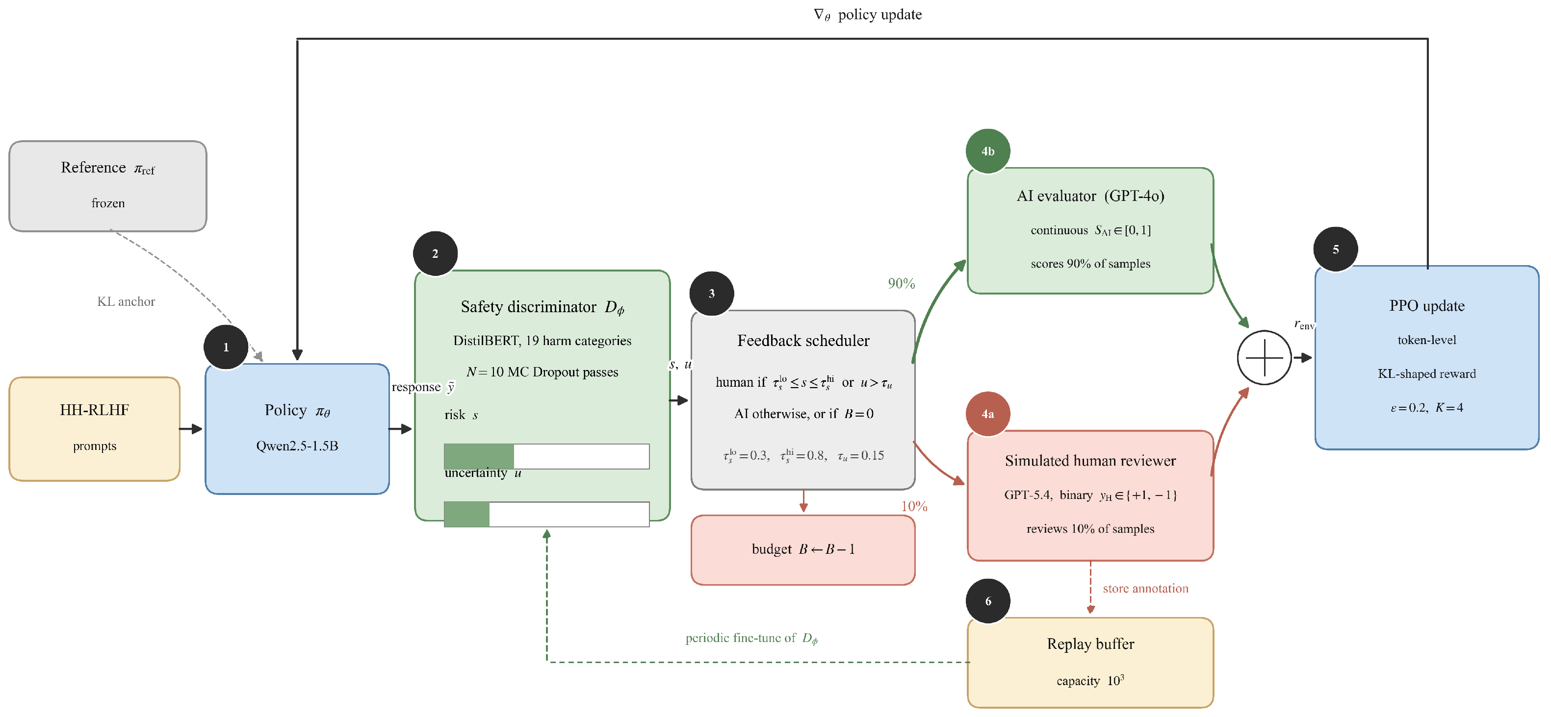
Terminology, and what this paper does not claim. One clarification bounds every quantitative claim below. The reliable channel is called the human channel because that is the role it fills in the framework, but in every experiment reported here it is not a person: it is a stronger language model prompted to behave like a careful senior safety reviewer (Appendix C). We therefore write simulated human feedback for what it produces, and every statement in this paper about budgets, savings, and safety parity refers to simulated human feedback, not to annotation by real people. Whether the same routing rule pays off with real annotators is an open question this paper does not answer; Section 5.5 states what answering it would need. No human subjects were involved.
This paper makes three contributions.
- This paper designs a routing rule that assigns each training sample to human or AI feedback according to the discriminator’s predictive uncertainty, so the two sources are mixed per sample rather than chosen once for the whole run (Section 3.4). The decision is recomputed inside every PPO iteration on the current policy’s outputs.
- This paper repurposes a fine-grained, multi-category risk representation, originally an offline classification target in PKU-SafeRLHF [32], as the per-step routing and uncertainty signal inside the reinforcement learning loop (Section 3.3). This is what makes category-level risk assessment, rather than a single binary, available to the routing decision at every policy-optimization step.
- This paper shows that, on two safety dialogue benchmarks, PKU-SafeRLHF and HH-RLHF, Hybrid RLHF-AIF reaches the discriminator-measured safety level of full simulated-human RLHF under a moderate Kullback–Leibler (KL) penalty while spending only 10% of the simulated-human feedback budget. The primary comparison is run over five random seeds on a 300-prompt test set and reported with confidence intervals and significance tests (Section 4.1). Ablations confirm that the uncertainty signal, the dynamic scheduler, and experience replay are each needed to preserve utility, while safety is maintained by the discriminator in every variant (Section 4.3). Because the routing discriminator would otherwise be both the target of optimization and the judge of it, every final policy is additionally re-scored with an independent safety evaluator, and both the utility judge and the AI-feedback channel are replaced by Claude Opus 5, a model from a different vendor; the ordering of methods survives both changes (Section 4.9 and Section 4.10).
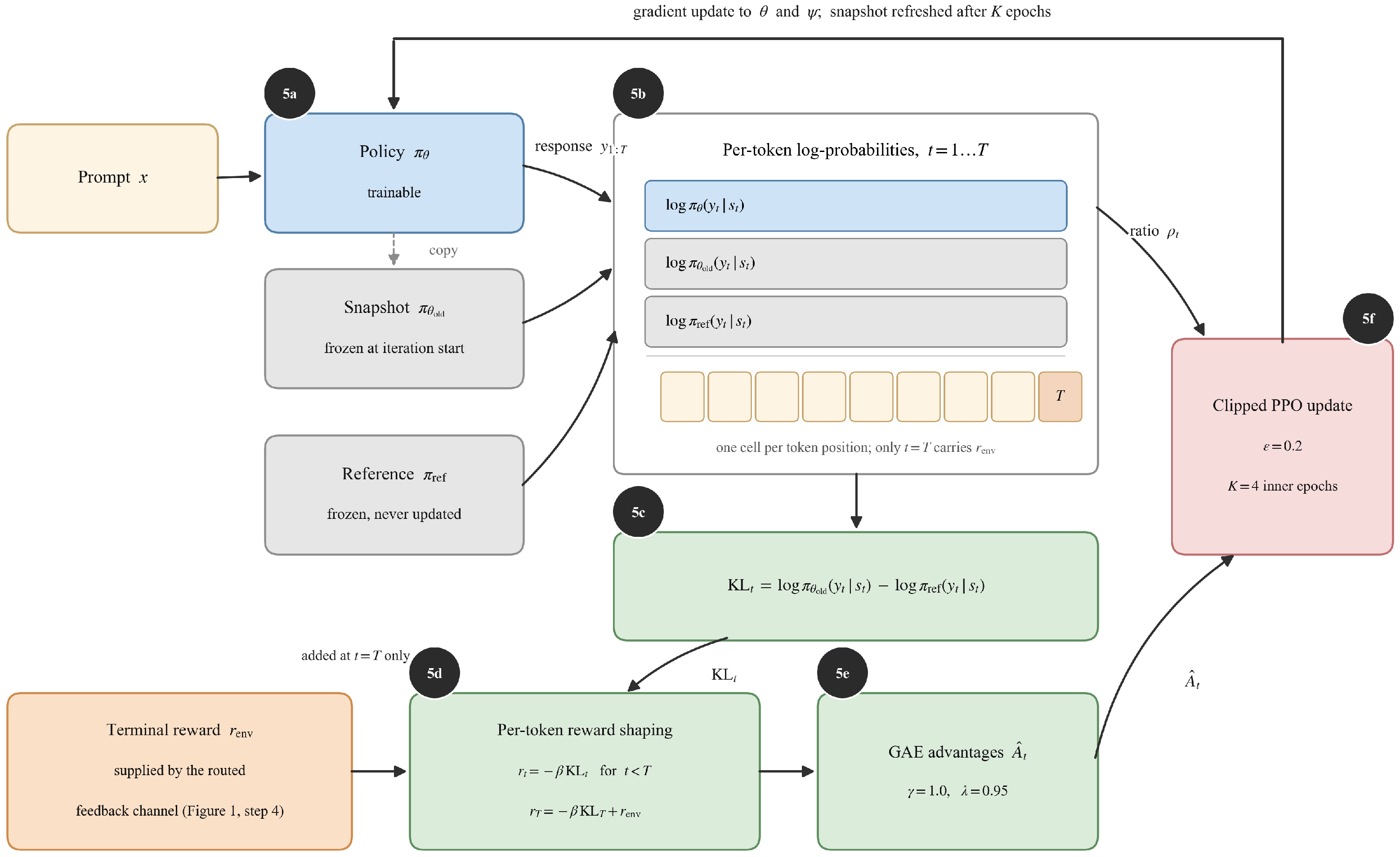
Figure 2.
Internal mechanics of step (5) of Figure 1, the PPO update. This figure expands the optimizer and contains no routing: the routing decision has already been made upstream, and enters here only through the single scalar at the bottom left. Reading it in order: (5a) the prompt is answered by , and a frozen snapshot is taken at the start of the iteration; (5b) per-token log-probabilities are collected under , , and the frozen reference ; (5c) their difference gives the per-token KL penalty; (5d) the terminal reward supplied by the scheduler is added at only, producing the shaped rewards of Equation (14); (5e) GAE with and turns those into advantages ; (5f) the clipped PPO objective (, inner epochs) updates , after which the snapshot is refreshed. Assigning KL-shaped rewards at every token position is what lets GAE propagate the terminal safety signal across the full response.
2. Related Work
From human to AI supervision, and the limit of each step. Policy-gradient reinforcement learning, from the REINFORCE estimator [33] through trust-region methods [34] to PPO [35], underpins modern alignment, and the cost of human feedback has driven a sequence of increasingly automated methods [36,37]. RLHF trains a reward model on pairwise human comparisons and optimizes the policy with PPO [6,20,21,22], and the recipe scales to production assistants [3,38]; its limitation is the one that motivates this paper, namely that annotation cost grows linearly in the number of samples, so the method does not scale to the sample volume that on-policy reinforcement learning consumes. Constitutional AI [23] and RLAIF [24] remove that cost by replacing human labels with model-generated evaluations, and pay for it with an evaluator bias that no later stage of the pipeline can detect or repair once training has begun [25]. A parallel line removes the on-policy stage instead: Direct Preference Optimization (DPO) [39] reparameterizes the reward through the policy, and its successors refine the objective [40,41,42,43]. Because these methods consume a fixed preference set offline, the question of which sample deserves which annotator never arises during training, which is exactly where our mechanism operates, and is also why they are not a drop-in baseline for it (Section 5.3). Safe RLHF [44] keeps reinforcement learning and adds an explicit safety constraint, but leaves the feedback source fixed. Making automated supervision more trustworthy from the inside has also been tried, by having models critique their own or one another’s output [45,46,47,48] and by separating drafting from verification across agents [49], which is cheapest wherever an automatic verifier exists, as in code and other executable artifacts [50,51]. Those signals establish whether an output is correct; they say nothing about how far an automated safety judgment can be trusted, which is the quantity our scheduler routes on. Every step that removes human involvement removes a layer of reliability, and the resulting open problems are documented in detail [18]. RLTHF [26] reverses the trend by reintroducing human annotation on the samples an AI labeler is most likely to mislabel, recovering full-human alignment quality with 6% to 7% human effort; its limitation is timing, because the selection is computed once, before training, from a static reward-model signal, and so cannot react to the distribution shift that on-policy optimization creates. Our work differs precisely there: the decision is made inside each PPO iteration from the discriminator’s predictive uncertainty on the current policy’s own outputs. Table 1 places the methods side by side.
Table 1.
Where Hybrid RLHF-AIF sits among alignment methods that use human, AI, or mixed feedback. “Routing decided” is the moment at which the human-versus-AI assignment of a sample is fixed, and “n/a” marks methods that draw on a single feedback source, for which no such decision exists. “Uses u” asks whether the assignment is driven by an evaluator uncertainty estimate; RLTHF selects on a static reward-model score instead. “Tracks drift” asks whether the selector is updated as the policy distribution moves, which in our case happens through experience replay. As in the rest of this paper, and as in RLTHF, the human channel of the mixed-feedback rows is simulated by a language model in the reported experiments.
Safety taxonomies and classifiers, and where their signal is consumed. Weidinger et al. [17] laid the groundwork with a taxonomy of LLM risks spanning hate speech, misinformation, and self-harm, and Ji et al. [32] turned a taxonomy into labeled data, annotating responses along 19 harm categories with pairwise preferences and using those labels to decouple helpfulness from harmlessness. Inan et al. [53] pushed safety classification to runtime with an LLM input and output guard, and large-scale moderation classifiers follow the same inference-time philosophy [54]; the same filtering problem reappears once the artifact is not plain text, as in automatically produced movie audio description [55]. Complementary benchmarks measure harmful or untruthful behavior [56,57,58], and red-teaming, by humans [59] or by other language models [60,61], surfaces the failures such classifiers must catch. The limitation these methods share is not accuracy but placement: the signal is consumed offline for labeling, or at inference time for filtering, so a multi-category risk vector is never fed back into policy optimization, and no confidence estimate is exposed that a training loop could act on. Our framework does both, driving per-step routing from the same 19-category schema while the scalar reward comes from the routed feedback source. Because the discriminator runs at every step, we keep it lightweight, in the spirit of efficient neural text classifiers [62,63] and of the wider efficiency push behind spike-based machine intelligence and spiking transformers [64,65,66].
Uncertainty in reward models. Estimation methods in this line have grown lighter over time, and each carries a cost. Gleave and Irving [67] tried full ensembles and found that models sharing a pretrained backbone produce too little diversity to be useful. Coste et al. [27] kept the ensemble and asked instead what the uncertainty means, showing that reward uncertainty tracks overoptimization risk, a phenomenon also captured by scaling laws for reward-model overoptimization [30] and formalized as reward hacking [31]; ensembling mitigates but does not remove the failure [68,69], and its memory and compute cost scale linearly with ensemble size. Yang et al. [70] replaced the ensemble with a Bayesian approximation over low-rank weights (Laplace-LoRA), which cuts cost and reduces reward hacking, at the price of an approximation whose quality is hard to audit under distribution shift. Dwaracherla et al. [52] used epistemic uncertainty to choose which samples to annotate next, the closest prior use of uncertainty to act during training; it selects which samples to label, whereas our scheduler decides, per sample and online, which of two reward sources scores it inside each PPO update. Our estimate builds on classical tools for predictive uncertainty and calibration in deep networks, namely MC Dropout [28], deep ensembles [71], the aleatoric–epistemic decomposition [29], and modern calibration analysis [72]. The limitation common to all of them, in this application, is that uncertainty is measured and reported but never used to change what happens during training. Section 3.3.3 states which estimator we use, why, and what it costs relative to these alternatives.
Evaluating and judging large language models. Because human evaluation is costly, current practice uses strong LLMs as judges, an approach validated by MT-Bench and Chatbot Arena [73,74] and surveyed in detail [75], alongside benchmarks that probe capability and behavior along many axes at once and settings in which a model plans or critiques generation itself [48,76,77,78,79,80,81,82,83,84,85,86,87]. The limitation this literature identifies is that a judge inherits the preferences of its own model family, so an overlap between judge and reward model inflates measured quality. We adopt the LLM-as-judge protocol for both the simulated human reviewer during training and the utility scoring at evaluation, keep the evaluation judge distinct from the AI-feedback model, and quantify the residual dependence in Section 5.4.
Safety supervision beyond plain text. Generative modeling now reaches images, video, radiance-field and splat-based scenes, and articulated human assets [88,89,90,91,92,93,94,95,96,97,98,99,100,101,102,103,104,105,106,107,108,109,110,111,112,113,114,115,116,117,118,119,120,121,122,123,124]. On the image side, filtering has been attempted by steering the sampling trajectory away from inappropriate content [125] and by erasing a concept from the weights [126], and both are circumventable under adversarial prompting [127]. None of these pipelines exposes a graded, multi-category safety signal comparable to the text-side taxonomies above. We therefore make no claim that the routing mechanism studied here transfers to those modalities, and state the boundary explicitly in Section 5.5.
3. Materials and Methods
The analysis in Section 1 calls for a framework that does three things: score each response along multiple safety dimensions, measure how much the scorer trusts its own output, and use that trust level to decide, at every training step, whether a sample needs human review or can be handled by the AI. This section describes how we build each component and connect them into a single training loop.
3.1. Problem Formulation and Framework Overview
We frame safety alignment as a token-level Markov decision process. Given a dialogue context x drawn from a prompt distribution , the policy generates a response autoregressively, where each token is sampled from the vocabulary . At decoding step t, the state is the concatenation of the context and the tokens emitted so far, , the action is the next token , and the transition is deterministic, . The episode terminates when an end-of-sequence token is emitted or the length cap is reached. A feedback process assigns a terminal scalar reward , and the policy is optimized to maximize the expected reward under a Kullback–Leibler (KL) trust region around a frozen reference policy :
In Equation (1), denotes the trainable parameters of the policy; is the expectation taken over prompts x drawn from the prompt distribution and over responses sampled from the policy ; is the terminal scalar reward returned by the feedback process for the pair ; T is the number of tokens in the generated response; is the Kullback–Leibler divergence between the policy and the frozen reference distribution at state ; is that frozen reference policy, which is never updated; and is the penalty coefficient that controls the strength of the reference anchor, with larger keeping the policy closer to . The novelty lies not in the optimizer but in how the terminal reward is produced: a learned safety discriminator scores every response, and an uncertainty-guided scheduler decides, per sample, whether comes from a human reviewer or an AI evaluator. Table 2 summarizes the notation used throughout this section.
Table 2.
Notation used in Section 3.
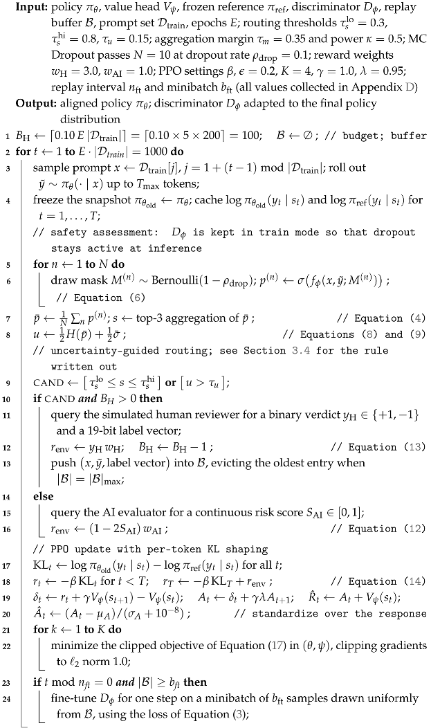
The key design choice is to place the routing decision inside each PPO iteration, so it responds to the current policy’s outputs rather than to a static pre-training split. Each iteration proceeds as follows. Given a prompt sampled from HH-RLHF, the policy generates a candidate response. The safety discriminator scores the response across 19 harm categories and aggregates the scores into a single risk value. MC Dropout estimates the discriminator’s confidence in that value. The feedback scheduler then routes the sample to a human reviewer or an AI evaluator based on the risk value and the uncertainty. The resulting reward feeds into a per-token-shaped PPO update that propagates the safety signal to every token in the response. Because the discriminator and scheduler run on every batch, the routing adapts automatically as the policy improves: samples that were ambiguous early in training may become clearly safe or clearly dangerous later, with no manual threshold change. Algorithm 1 summarizes the loop, and Figure 1 illustrates it.
Three implementation details are worth stating explicitly, because they are the ones a reimplementation is most likely to get wrong. First, the discriminator is left in training mode during the N MC Dropout passes, but its parameters are not updated there; only the replay step at the end of the iteration writes to . Second, the KL term is computed once, on the rollout snapshot , and reused across all K inner epochs, so the shaped reward is a constant of the iteration rather than a function of the parameters being optimized. Third, the budget counter is a single scalar allocated once for the entire run rather than per epoch: at 200 prompts over epochs, the run performs 1000 rollouts, and a 10 percent cap gives reviewer queries in total, not 20 per epoch. An iteration that finds no candidate therefore does not forfeit its share, and the cap binds across epochs. should not be confused with the replay buffer , which is a set of stored annotations with its own capacity ; every reviewer query decrements by one and appends one entry to , so over a full run receives at most 100 of its 1000 slots and never fills. Appendix H shows the resulting consumption profile.
3.2. Data Construction
Training the framework requires two separate pools of data: one to teach the discriminator what unsafe responses look like, and one to give the policy realistic prompts to respond to. We use PKU-SafeRLHF [32] for the first role because it is the only public dataset that provides per-response binary labels across 19 harm categories, the granularity our multi-label discriminator needs. We use HH-RLHF [19] for the second role because its multi-turn dialogues supply the context-rich prompts that stress-test safety in realistic settings. The two datasets are deliberately kept apart. The discriminator is pretrained exclusively on PKU-SafeRLHF and never sees HH-RLHF response patterns during pretraining, which makes generalization to policy-generated responses a necessary condition for stable training rather than an artifact of overlapping distributions.
3.2.1. PKU-SafeRLHF for Discriminator Pretraining
A binary safe or unsafe label cannot tell the policy what is wrong with a response, only that something is. If a reply contains both hate speech and self-harm content, a single bit loses the distinction, and the policy receives the same gradient whether it fixes one problem or both. We therefore train the discriminator as a multi-label classifier over all 19 harm categories defined in PKU-SafeRLHF [32]; the full category list is given in Appendix A.
| Algorithm 1: Hybrid RLHF-AIF, the complete training run over E epochs |
 |
Each sample in the dataset pairs a prompt with two candidate responses, each annotated with a 19-dimensional binary risk label (one bit per harm category) together with human safety and helpfulness preference rankings over the pair. During preprocessing, we split the two candidates into independent prompt and response pairs, which doubles the number of training examples. Each of the 19 harm dimensions is modeled as an independent probability through a sigmoid output, producing a 19-dimensional risk vector per response. Although the ground-truth labels are binary, the continuous formulation lets the discriminator express partial confidence, for instance scoring a borderline response at rather than committing to 0 or 1. For downstream use in the scheduler and PPO, the 19 probabilities are aggregated into a single scalar risk score , detailed in Section 3.3.2.
3.2.2. HH-RLHF for Policy Exploration
Safety risks in dialogue often emerge from context: a reply that is harmless in isolation can become dangerous when it follows a manipulative prompt history. To expose the policy to this kind of risk, we draw prompts from HH-RLHF [19], a multi-turn dialogue preference dataset, and discard all reference responses so that the policy must generate its own. We extract the full dialogue history and truncate it at the final Assistant: turn to form the context state x. The policy then generates a candidate response , and the pair is concatenated and fed to the pretrained discriminator for risk scoring. Because the discriminator sees the multi-turn context, up to the 256-token input cap of Section 3.6, it can catch risks that a single-turn evaluator would miss, for example, a response that complies with a gradually escalating harmful request.
3.3. Uncertainty-Aware Safety Discriminator
The discriminator must do two things that a standard classifier does not: score a response across 19 harm categories in a single forward pass, and report how confident it is in that score. The first requirement drives the architecture; the second is handled by MC Dropout (Section 3.3.3).
3.3.1. Multi-Label Architecture and Training
We fine-tune a DistilBERT [62,128] backbone for multi-label classification. DistilBERT is a knowledge-distilled version of BERT that retains 97% of its language-understanding performance on the GLUE benchmark while using only 60% of the parameters [62]. We choose it over full BERT because the discriminator runs on every sample at every PPO iteration, and each sample requires MC Dropout forward passes; with full BERT, this would roughly double the discriminator’s per-sample inference cost. The accuracy trade-off is acceptable because our task is binary multi-label classification, which demands less capacity than open-ended language understanding, and the 10 passes are averaged before any decision is made, smoothing out small per-pass errors.
Given a prompt and a policy-generated response, we concatenate them with a [SEP] token and feed the sequence into the backbone. The model produces a logit vector , one coordinate per harm category, and per-category violation probabilities are obtained through the sigmoid function:
where i indexes the 19 harm categories of Appendix A; is the i-th coordinate of the logit vector z produced by the DistilBERT backbone for the concatenated prompt and response; denotes the logistic sigmoid function; is the natural exponential; and is the resulting predicted probability that the response violates category i. The 19 outputs are independent, so is not constrained to one.
We train with binary cross-entropy rather than a softmax loss, because the 19 categories are not mutually exclusive: a single response can violate several at once, and softmax would force the probabilities to sum to one, suppressing co-occurring violations. The loss is
where is the per-sample loss summed over all 19 categories; is the ground-truth label for category i, equal to one when the response violates that category and zero otherwise; is the predicted probability of Equation (2); and is an inverse-frequency weight equal to the ratio of negative to positive samples for category i in the training set, clamped to that interval. The weight multiplies only the positive term, so rare categories are penalized more heavily when missed. This reweighting prevents the optimizer from ignoring rare but serious categories such as self-harm or human trafficking, which together make up less than 4% of positive labels. The discriminator is pretrained once for three epochs with the AdamW optimizer, a learning rate of , a warmup ratio of , and a batch size of 8, on up to 20,000 training and 2000 evaluation prompt and response pairs. It is then frozen as the starting point for every reinforcement learning run, so that performance differences across runs reflect the feedback-routing strategy alone.
3.3.2. Risk Score Aggregation
The scheduler needs a single scalar, but naively averaging all 19 category probabilities would dilute a strong signal in one or two categories across 17 near-zero ones: a single maximally violated category would contribute only to the mean. We therefore restrict the aggregation to the three highest-probability categories, apply a margin threshold to suppress weak activations, and compress the remaining signal with a concave power transform:
where is the aggregated scalar risk score of the pair ; denotes the index set of the three categories with the largest predicted probabilities ; is the weight of category i and W is their sum, which normalizes the result; clips negative arguments to zero, so a category contributes nothing unless exceeds the margin; is that margin threshold, and dividing by rescales the surviving range back to ; and is the concave power exponent (distinct from the PPO discount factor of Section 3.5). The margin removes categories with , which typically reflect noise rather than genuine risk; the concave power amplifies moderate-confidence predictions that would otherwise be too low to trigger routing. The category weights are set uniformly to one, so . Non-uniform emphasis on rare categories is instead injected during training, through the inverse-frequency weights in the binary cross-entropy loss of Equation (3), which keeps the aggregation stage simple and interpretable.
Because the denominator is the fixed sum over three categories, s is calibrated to the number of co-occurring harms rather than to a single worst case: a harm concentrated in one category saturates near , two simultaneous harms near , and only three or more reach the upper band. This is a deliberate but consequential choice, since it bounds what the scalar can express, so we state the alternatives and the trade-off explicitly. Writing for the margin-and-power transform of category i, four aggregation rules are natural:
where is the rule of Equation (4) that we use; is maximum risk, which reaches 1 on a single maximally violated category; is a severity-weighted maximum in which encodes how serious category i is judged to be; and is a noisy-OR that treats the categories as independent evidence and therefore rises with both the severity and the number of active categories. Maximum risk and noisy-OR remove the saturation and would give a lone severe harm the score it intuitively deserves; the price is that they inherit the discriminator’s per-category false positives directly, since one over-confident category is enough to saturate the score, whereas averaging over the top three suppresses isolated errors. Severity weighting is the principled middle ground but needs a defensible , which is a value judgment that PKU-SafeRLHF does not supply and that we were not willing to invent. A learned aggregator is a further option, and it needs labels on policy-generated responses that we do not have.
Three points bound what our choice costs. First, the routing thresholds , and the violation cut-off of Section 3.6 are calibrated on this scale, so swapping the rule is not a drop-in substitution: it requires recalibrating all three, and a comparison that changed the aggregation while holding the thresholds fixed would measure the mismatch rather than the rule. Second, a severe single-category harm is not silently lost, because it can still reach the reviewer channel through the uncertainty condition , and because the AI and human evaluators on both paths read the full response rather than the scalar. Third, the effect is one-sided: saturation can under-route a severe single-category harm to the reviewer, never over-route it. We report the fixed-denominator rule as the configuration actually used, do not claim it is the best of the four, and list the matched comparison of Equation (5) under recalibrated thresholds as a concrete item in Section 5.6.
The same argument applies to the scalar gate itself, which collapses a 19-dimensional signal into a single number. It is worth being precise about what is collapsed. The full risk vector is retained and is what the reviewer channel labels and what the replay buffer stores; only the routing gate is scalar. A category-specific gate, for example a per-category band or a rule that escalates whenever any high-severity category exceeds a low threshold, would let the reviewer budget be steered toward the categories where reviewer judgment is worth most. That is a strict generalization of Equation (10), and it multiplies the number of hand-set thresholds by 19, which is why we did not adopt it here without a way to fit them; Section 5.6 states it as the natural next step once per-category error rates on policy rollouts are available.
3.3.3. Monte Carlo Dropout Uncertainty
A single forward pass gives a point estimate of the risk score but says nothing about whether the discriminator trusts that estimate. We need a confidence measure that is cheap enough to compute on every sample at every PPO iteration. Ensemble methods, the standard choice in prior work [27,67], would require maintaining multiple copies of the discriminator, multiplying memory and compute by the ensemble size. MC Dropout [28] avoids this: it reuses the same model with dropout layers kept active at inference time and runs N stochastic forward passes with independently sampled dropout masks. We use a distinct symbol N for the number of passes to avoid confusion with the response length T of Section 3.5. Formally, let denote the discriminator evaluated with a binary dropout mask M whose entries equal 1 (keep) with probability and 0 otherwise, where is the DistilBERT dropout rate. For pass , we sample a fresh mask and obtain a probability vector
where n indexes the stochastic forward pass; is the binary dropout mask drawn for that pass, each of whose entries is an independent Bernoulli variable equal to one with keep probability ; is the logit vector produced by the discriminator with parameters evaluated on the pair under that mask; is applied coordinatewise; and is the resulting per-category probability vector for pass n. Equation (6) is the Monte Carlo estimate of the posterior predictive distribution under a Bernoulli variational approximation [28]. From the resulting set we compute a mean vector and two complementary uncertainty terms:
where is the number of MC Dropout passes; is the elementwise mean probability vector over those passes, used as the discriminator’s point prediction; u is the combined scalar predictive uncertainty; is the normalized binary entropy term defined in Equation (8); is the mean per-category dropout standard deviation defined in Equation (9); and the two coefficients weight the two terms equally. The first term is the normalized binary entropy of the mean probabilities, averaged over the 19 categories,
where is the i-th coordinate of , is the base-2 logarithm so that each per-category term lies in , and the factor averages over the categories. The convention is used at the endpoints. This term is high when sits near , and the discriminator cannot decide. The second term
is the average per-category standard deviation across the N passes, where is the probability assigned to category i on pass n and the inner square root is the population standard deviation of that category over the passes. This term is high when different dropout masks disagree. The two terms are combined because they catch different failure modes. A response can have low variance across dropout passes yet still sit at for a dangerous category: the model gives the same answer every time, but that answer is undecided, and entropy catches this. Conversely, a response can have a confident mean prediction yet show high variance across passes: the average looks decisive, but individual passes disagree, and the standard deviation catches this. Using only one term would miss the other case. We weight both equally at for simplicity; the threshold in the scheduler absorbs any calibration difference between the two scales. The scalar risk score is computed from through Equation (4) and, together with the combined uncertainty (since and ), is passed to the scheduler as the routing signal. We stress that s and u govern routing only; the scalar reward that the policy is trained on comes from the routed feedback source (Equations (12) and (13)), not from the discriminator.
We set because the discriminator already runs inside every PPO iteration, so multiplies per-sample discriminator inference cost by ten, which remains tractable with DistilBERT. Higher values such as , used by Gal and Ghahramani [28] in offline settings, would sharpen the variance estimate but slow training proportionally, reducing the number of PPO iterations within the same wall-clock budget. Because our goal is not a calibrated posterior but a ranking of samples by relative uncertainty for routing, the variance from 10 passes is enough to separate high-uncertainty samples from low-uncertainty ones.
Why MC Dropout, and what it gives up. MC Dropout is the least sophisticated of the available estimators, and it is fair to ask whether a safety-critical routing decision should rest on it, so we state the comparison and the claim precisely. Table 3 lists the four candidates with their per-sample cost inside the loop, expressed in units of one DistilBERT forward pass, which is the quantity that matters when the estimator runs on every sample of every PPO iteration. A deep ensemble of M independently initialized discriminators [71] gives the strongest disagreement signal, but multiplies both memory and compute by M, and Gleave and Irving [67] found that ensembles sharing a pretrained backbone, which is our situation, yield too little diversity to justify that factor. A Laplace approximation over low-rank weights [70] is far cheaper at inference but requires a curvature estimate that must be refreshed whenever the discriminator is fine-tuned from the replay buffer, so its cost is tied to the replay schedule rather than being a constant. BALD, the mutual-information criterion, is the estimator that would actually separate epistemic from aleatoric uncertainty, and it is computed from the same N stochastic passes we already draw, so it is nearly free given our setup; it is the alternative we consider most worth testing next, and we say so in Section 5.6.
Table 3.
Uncertainty estimators for a discriminator that runs on every sample of every PPO iteration. Cost is the per-sample cost inside the training loop, in units of one DistilBERT forward pass; N is the number of stochastic passes and M the ensemble size. The last column states what the estimator buys that MC Dropout does not.
Our claim about u is deliberately narrow. We do not claim that MC Dropout with yields a calibrated epistemic uncertainty; it does not. The combined u is a predictive uncertainty in which the entropy term captures total uncertainty and the dropout-variance term captures model disagreement, without separating the two, and because all N passes share one backbone, the estimate can understate model uncertainty exactly where the policy has drifted furthest from the discriminator’s training distribution. What the routing rule needs is weaker than calibration: it needs u to rank samples so that the discriminator’s own errors concentrate in the high-u tail. That is a testable property, and Section 4.4 tests it directly, reporting the error-detection AUROC of u and the share of errors falling in the most uncertain fifth of the test split. We therefore treat u as a validated routing heuristic and not as a Bayesian posterior, and we read the results of Section 4.6 as evidence about the value of routing on some error-correlated signal rather than about the optimality of this particular estimator.
3.3.4. Experience Replay
As the policy improves, the distribution of responses it generates shifts, and risk patterns that were common early in training may become rare. If the discriminator is never updated, its predictions gradually drift away from the actual policy distribution. To keep the discriminator current, we store every simulated-human annotation collected during training in a replay buffer and periodically sample from it to fine-tune the discriminator with the same binary cross-entropy loss of Equation (3). The buffer holds up to samples. A smaller buffer would make successive training batches too similar, hurting gradient diversity; a larger one would retain too many annotations from earlier, weaker versions of the policy, pulling the discriminator toward an outdated distribution. At , the buffer covers several full episodes while still reflecting recent policy behavior.
Drift and forgetting over long runs. Replay is a mechanism for tracking drift, and any mechanism that tracks drift can also forget. Two failure modes are possible in principle. The first is catastrophic forgetting of the PKU-SafeRLHF pretraining distribution: because the replay batches contain only policy-generated responses labeled by the reviewer channel, repeated fine-tuning pulls toward the current policy and away from the taxonomy coverage the discriminator was originally trained for, so rare categories that the policy has stopped producing could decay first, which is the opposite of what the inverse-frequency weighting of Equation (3) is meant to achieve. The second is a self-confirming loop: the reviewer channel sees only the samples the discriminator flagged, so replay retrains the discriminator on its own referral distribution and can narrow rather than correct it.
At the scale of the runs reported here, neither mode is exercised, and we prefer to say that plainly rather than claim robustness we have not measured. With a 10% cap over 1000 steps, the buffer receives at most about 100 annotations, never reaches its capacity, and drives on the order of tens of single-step updates; that is far too little to overwrite a backbone fine-tuned for three epochs on up to 20,000 pairs. The consequence is that our experiments demonstrate that replay helps over this horizon, which the ablation of Section 4.3 shows, but they do not establish stability over the much longer runs a production deployment would use. Two standard mitigations apply directly and cost little, and we recommend both for such runs: mix a fixed fraction of the original PKU-SafeRLHF training data into every replay batch, so the pretraining distribution is rehearsed alongside the new annotations, and hold out a frozen slice of the PKU-SafeRLHF test split as a regression monitor, re-evaluating per-category F1 after each replay update and stopping the update stream if any category degrades beyond a set tolerance. A regularization-based alternative, such as an elastic-weight penalty anchored at the pretrained , would achieve the same end at the cost of one extra hyperparameter. Measuring long-horizon replay stability under these mitigations is stated as future work in Section 5.6.
3.4. Uncertainty-Guided Feedback Scheduler
The discriminator produces a risk score and an uncertainty estimate for each sample, but these numbers alone do not decide anything. The scheduler reads both and makes the routing decision. The AI path handles a sample by itself only when the discriminator has no reason to doubt its own judgment: the response is clearly safe (low risk, high confidence) or clearly dangerous (high risk, high confidence). In all other situations, namely ambiguous risk, low confidence, or both, the sample becomes a candidate for human review:
Here is a Boolean flag marking the sample as eligible for human review; is the aggregated risk score of Equation (4) and the combined uncertainty of Equation (7); and are the lower and upper bounds of the ambiguous risk band; and is the uncertainty threshold above which the discriminator is deemed not to trust its own prediction. The two conditions are joined by a logical or, so either ambiguity alone or low confidence alone is sufficient.
A candidate is routed to the reviewer channel only if the simulated-human budget has not been exhausted:
where names the feedback channel that scores the sample, and budget is the counter of Algorithm 1, initialized once per run to 10 percent of the total number of rollouts, , and decremented by one each time a sample is sent to the reviewer channel. Once reaches zero, every remaining sample falls back to the AI channel.
The budget cap prevents the candidate pool from over-consuming reviewer resources; Appendix H shows that the budget is consumed steadily throughout training. Table 4 writes the rule out case by case.
Table 4.
The routing rule of Equations (10) and (11), written out. Here, s is the aggregated risk score of Equation (4) and u the combined uncertainty of Equation (7). The three thresholds are , the lower edge of the ambiguous risk band; , its upper edge; and , the confidence cut-off above which the discriminator is treated as not trusting its own prediction. The last row applies once the budget counter B of Equation (11) reaches zero.
How the three thresholds were set, and how much they matter. The two risk thresholds are not free parameters but are read off the scale that Equation (4) defines. Because the denominator is fixed at three categories, a harm concentrated in one category saturates near and two co-occurring harms near . Setting therefore places the lower edge just below single-category saturation, so that any response the discriminator considers a genuine single-category violation enters the ambiguous band, and setting places the upper edge above the two-category level, so that only responses with three or more co-occurring harms are treated as confidently unsafe. Both follow from the aggregation rule rather than from tuning on results. The uncertainty threshold has no such derivation from the risk scale. It was set by hand and, as it turns out, coincides with the midpoint of the mean uncertainty on correctly classified responses and on misclassified responses that Section 4.4 measures on the held-out PKU-SafeRLHF split ( and ), which is where one would place a cut to separate those two populations; it was not tuned against any policy-level utility or safety metric. These cutoffs are conceptually parallel to, but not numerically identical to, the five-level rubric the AI evaluator applies to its own independent score (Appendix B), which operates on a different scoring function.
We did not run a three-dimensional sweep over , and the reported results should not be read as evidence that this triple is optimal. Two structural features limit how much the choice can matter, and we set them out so the reader can judge the exposure. First, the budget cap, not the thresholds, is the binding constraint: the thresholds determine which samples are eligible for the reviewer channel and in what order they consume the counter, but the total volume of reviewer feedback is fixed at 10% by B regardless of where the thresholds sit. Loosening them enlarges the candidate pool and makes the channel first-come-first-served over a broader set; tightening them shrinks the pool and, if it shrinks below the budget, leaves part of the budget unspent, which Appendix H shows happens only marginally at . Threshold changes therefore mostly reorder which samples receive the fixed budget rather than change how much is spent. Second, the routing-strategy comparison of Section 4.6 varies the allocation rule far more aggressively than any threshold shift could, holding the budget at 10% while replacing uncertainty-guided routing with risk-only, static, and random allocation, and the utility gap it measures is an order of magnitude larger than the differences a threshold perturbation would plausibly produce. A proper sensitivity study remains desirable, and Section 5.6 specifies the grid we would run.
Once a sample is routed, the two paths produce rewards in different forms. The AI path uses an independent LLM safety evaluator that reads the full prompt and response and outputs a continuous risk score (the prompt is reproduced in Appendix B). A safe response should receive a positive reward and a dangerous one a negative reward, so we apply an affine map that sends to with the midpoint mapped to zero:
where is the scalar reward delivered by the AI channel, is the risk score returned by the LLM safety evaluator (0 meaning fully safe and 1 fully unsafe), and is the AI reward weight. The factor performs the affine map from to , so a safe response yields a positive reward and a dangerous one a negative reward.
The human path works differently. The reviewer sees the same prompt and response pair but returns a binary verdict for safe or unsafe, and the reward is
where is the reward delivered by the reviewer channel, is the reviewer’s binary verdict ( for safe, for unsafe), and is the human reward weight. Whichever of and the scheduler selects becomes the terminal reward of Equation (1).
The AI reward is continuous because the evaluator can express degrees of risk; the human reward is binary because, on the ambiguous samples that reach this path, a simple safe-or-unsafe verdict is more useful to the policy than a noisy score. We set and . Human annotations make up a small fraction of all rewards, so each one must carry more weight to avoid being drowned out by the larger volume of AI scores. At , a single human label exerts roughly the same gradient influence as three AI scores, giving human feedback an effective share of the policy update that is proportional to its reliability advantage rather than to its sample count. If both weights were equal, the policy update would be dominated by AI feedback on easy samples, and the sparse human corrections on ambiguous cases would have little effect on the gradient.
3.5. Token-Level Reward Shaping for PPO with Hybrid Rewards
Standard PPO for language models assigns a reward only at the last token of the generated response, treating the entire sequence as a single action. This makes it hard for the policy to learn which tokens caused a response to be judged safe or unsafe. We instead apply reward shaping at every token position, following Ouyang et al. [6] and the earlier KL-controlled sequence generation of Jaques et al. [129]: each non-terminal token receives a KL penalty that discourages the policy from drifting too far from the frozen reference model , and the terminal token additionally receives the environment reward from the feedback scheduler:
where is the shaped reward assigned to token position t; T is the index of the terminal token of the response; is the single-sample estimate of the per-token KL divergence, evaluated once on the rollout snapshot rather than on the current policy so that it stays constant across the K inner epochs; is the same penalty coefficient as in Equation (1); is the full generated response; and is either from Equation (12) or from Equation (13), depending on the scheduler’s decision. Only the terminal position receives ; every other position receives the KL term alone.
A per-token value head , a linear projection of the policy’s last-layer hidden state, predicts the return at each position. Generalized Advantage Estimation (GAE) [130] then propagates the shaped reward backward through the response. Writing the temporal-difference residual as
where is the one-step temporal-difference error at position t; is the shaped reward of Equation (14); is the discount factor, set to because the episodes are finite; is the scalar value predicted by the value head with parameters at state ; and the boundary condition terminates the recursion after the last token. From these residuals, the advantage is accumulated by the backward recursion:
where is the GAE advantage at position t; is the GAE trace-decay parameter that trades bias against variance, set to ; initializes the backward recursion; and is the resulting value target used to regress the value head. The advantages are standardized across the response, , where and are the mean and standard deviation of and guards against division by zero. Let denote the importance ratio between the current policy and the rollout snapshot. The policy and value head are optimized jointly by minimizing the clipped PPO objective [35]
where is the joint loss over the policy parameters and the value-head parameters ; is the empirical average over all token positions in the rollout batch; is the importance ratio defined above and the standardized advantage; confines the ratio to the interval , and taking the minimum of the clipped and unclipped terms makes the objective a pessimistic lower bound that removes the incentive to move far from one; is the clip ratio; and is the coefficient weighting the squared value-regression error against the policy term. The objective is applied for K gradient epochs over each rollout, with gradients clipped to a global norm of . We use a clip ratio of , a value coefficient of , epochs, and GAE parameters and . The full hyperparameter table is given in Appendix D. Figure 2 illustrates how the per-token shaped rewards become GAE advantages and drive the clipped update.
On the choice of reward granularity. Equation (14) is one point on a spectrum, and it is worth saying which alternatives exist and what choosing among them would test, since we do not sweep them. At the coarse end, terminal-only reward places at with no KL shaping at intermediate positions, leaving GAE to propagate a single scalar backward through the whole response; this is the simplest option and the one most exposed to the credit-assignment problem that motivated our choice, because the value head must absorb the entire drift penalty. At the fine end, a dense process reward would score spans or sentences of the response separately, which localizes credit much more sharply but requires an evaluator willing to emit span-level safety judgments; neither the AI evaluator nor the simulated reviewer of Appendix C does, and asking a binary reviewer for span-level labels would change the annotation cost that this paper is trying to reduce. Our choice, per-token KL shaping with a terminal task reward, sits between the two and follows established practice for KL-controlled language generation [6,129]: it is exactly as informative as terminal-only reward about safety, since still arrives only at , and strictly more informative about drift, since the KL penalty is charged at the position where it is incurred rather than summed into the final step. Two consequences follow and both matter for reading our results. Because is evaluated on the rollout snapshot, the shaped reward is constant across the K inner epochs, which keeps the advantage targets stationary within an iteration. And because the safety signal itself remains terminal, the granularity choice is orthogonal to the routing question this paper studies: any of the three schemes would be driven by the same routed . We therefore do not claim that per-token KL shaping is optimal, only that it is the variant that isolates the routing mechanism, and Section 5.6 lists a granularity sweep as a separate question.
3.6. Experimental Setup
Environment. All experiments run on a single NVIDIA GeForce RTX 4080 SUPER GPU with 16 GB of memory, using PyTorch 2.5.1, Hugging Face Transformers 4.46.0, Accelerate 1.1.1, and CUDA 12.4. Training uses FP16 mixed precision. Prompts are processed in batches sized to fit 16 GB of memory (between 8 and 32 sequences depending on length), with a maximum sequence length of 256 tokens and a maximum generation length of 96 tokens. Seeding follows the two-tier design of the experiments rather than a single global value. The primary comparison of Section 4.1, and every study derived from it, retrains each configuration from scratch under five seeds, , with the seed controlling policy and value-head initialization, prompt order, rollout sampling, and MC Dropout masks; results are reported as means with standard deviations across those five runs. The secondary single-seed studies, namely the three-point KL sweep of Section 4.2 and the scaling study of Section 4.7, fix the seed to 42 so that methods are compared on identical prompts and identical sampling noise; we label these as single-seed wherever they are reported. Full details are in Appendix E.
Policy model. We use Qwen2.5-1.5B-Instruct [131] as the base policy, loaded from its publicly available instruction-tuned checkpoint. We choose this model because it is instruction-tuned out of the box, small enough to train on a single consumer GPU together with the MC Dropout overhead, and publicly available for reproducibility. Scaling to larger models is left as future work.
Training schedule. All runs share an identical PPO configuration except for the KL coefficient , which is the independent variable in our safety and utility analysis. Each run trains for 5 epochs over 200 prompts, giving 1000 per-sample rollouts in total (one rollout per prompt visit, each followed by an inner PPO update of epochs), with a learning rate of , a clip range of , and GAE parameters and . We test three values of : for weak regularization, for moderate, and for strong. The safety discriminator is pretrained once on PKU-SafeRLHF and shared across all runs without modification, so that performance differences reflect the feedback-routing strategy alone. Table 5 summarizes the per-run configuration.
Table 5.
Per-run configuration. The budget column is the share of training samples routed to the simulated human reviewer, which is a language model in all runs. All hyperparameters not listed (PPO settings, optimizer, hardware, discriminator backbone) are identical across runs. Each configuration is retrained under the five seeds of Section 3.6.
Baselines. To test whether selective, discriminator-based escalation justifies its labeling cost, we compare Hybrid RLHF-AIF against two baselines at opposite ends of the cost and reliability trade-off. In RLHF (upper bound), every training sample is reviewed through the reviewer channel, matching the conventional RLHF setup [6,19], except that the reviewer is simulated by GPT-5.4 rather than being a person, because real annotation across 1000 PPO steps is infeasible within a typical academic budget. This baseline consumes 100% of the labeling budget and serves as the full-supervision reference; throughout the paper we call it full simulated-human RLHF when the distinction matters. In RLAIF (lower bound), the reviewer channel is removed entirely, and all feedback comes from GPT-4o, following the Constitutional AI approach [23]; this baseline incurs no reviewer cost and serves as the zero-supervision reference. In Hybrid RLHF-AIF (ours), the AI evaluator is GPT-4o (the same model as in RLAIF) and the simulated human reviewer is GPT-5.4 (the same model as in RLHF), prompted as described in Appendix C; the scheduler of Section 3.4 decides which samples reach each channel, with the reviewer budget capped at 10% of training samples. One property of this design should be stated up front because it bounds the conclusions: GPT-4o and GPT-5.4 come from the same vendor and therefore share pretraining lineage, instruction-tuning conventions, and refusal style, so the two channels are less independent than the labels “AI” and “human” suggest. Section 5.4 quantifies what this leaves exposed, and Section 4.10 reports the evaluator-diverse replication itself, in which both the utility judge and the AI-feedback channel are replaced by Claude Opus 5, a model from a different vendor.
Evaluation protocol and metrics. Three held-out sets are used, all disjoint from the training prompts. A monitoring set of 8 prompts is evaluated every 100 training steps to track learning dynamics; a 32-prompt test set is used for the secondary KL sweep; and a 300-prompt test set is used for the primary comparison and every other study. For the 32-prompt sweep, all runs use the same prompt set and the same fixed random seed, which turns that comparison into a paired design over identical prompts and identical sampling noise, and its numbers should be read as a controlled comparison of the relative ordering of methods rather than as population estimates. Six metrics are reported along two axes. The three safety metrics are all computed by the safety discriminator, which is also the model that drives routing during training; we therefore write discriminator-measured whenever precision matters. Section 5.4 sets out what that circularity does and does not permit us to conclude, and Section 4.9 re-scores the same responses with an independent evaluator so that the two instruments can be compared directly. Safety metrics, for which lower is better, are the violation rate, defined as the fraction of test responses whose aggregated risk score is at least (this evaluation threshold is deliberately separate from the routing thresholds of Section 3.4, and , which govern training-time human escalation rather than test-time scoring); the average risk score from the discriminator; and a toxicity score computed by applying the aggregation of Equation (4) to the toxicity-related subset of categories (insulting behavior, discriminatory behavior, violence, sexual content, and psychological harm), in the spirit of toxic-degeneration evaluation [132]. Utility metrics, for which higher is better, are: helpfulness and naturalness, scored by GPT-5.4 acting as an LLM judge and reported as continuous values in averaged over the test set, so that the absolute magnitudes are small on these adversarial safety prompts and are meaningful chiefly in relative comparison across methods; and BLEU-4 [133] and ROUGE-L [134], computed against the withheld reference responses. The helpfulness and naturalness judge is the same model (GPT-5.4) as the simulated human reviewer, but the two roles differ: the reviewer produces a binary verdict on the roughly 10% of samples routed to it during training, whereas the evaluation judge scores quality on a continuous scale across all test samples. To limit reward hacking, the evaluation judge is kept distinct from the GPT-4o model used in the AI-feedback channel; it is not, however, independent of the reviewer channel or of the vendor behind both. Section 5.4 works through the direction in which that dependence can and cannot bias the reported comparison, and Section 4.10 measures it by re-scoring every response with Claude Opus 5, a judge from a different model family, under a byte-identical rubric. Because the reference responses are withheld during training and the policy generates its own answers, BLEU-4 and ROUGE-L reflect surface overlap with text the policy never optimizes toward; we therefore treat the LLM-judged helpfulness and naturalness as the primary utility signals and report BLEU-4 and ROUGE-L for completeness.
Ablation design. To quantify the contribution of each component, we conduct three ablations on Hybrid RLHF-AIF at its reference configuration (10% simulated-human budget, ), removing one component at a time while keeping the rest unchanged. Removing uncertainty estimation disables MC Dropout and uses a single deterministic forward pass, so routing falls back to the risk score alone and low-risk-but-uncertain samples are no longer flagged. Removing the dynamic scheduler replaces discriminator-based routing with fixed random allocation, where 10% of training steps are pre-assigned to the reviewer channel before training begins, which keeps the budget at 10% but removes targeting. This variant isolates the value of when the routing decision is made: like static, pre-training schemes, it fixes the human-versus-AI split before optimization rather than recomputing it on the current policy. We emphasize that it is not a reimplementation of RLTHF [26], which selects informative samples for human correction; random static allocation is a weaker, content-agnostic baseline, and a head-to-head comparison with RLTHF’s actual selection rule is left to future work. Removing experience replay freezes the discriminator at its pretrained state, so it cannot adapt to the shifting policy distribution. Results are reported in Section 4.3.
Which evidence is primary. The paper reports two tiers of experiments, and it matters which carries the argument. The primary comparison retrains every configuration at the operating point with five random seeds () and evaluates on the 300-prompt test set, reporting means, standard deviations, 95% confidence intervals, and significance tests (Section 4.1); all headline claims rest on it. The three-point KL sweep over described above is secondary: it is a single-seed, 32-prompt exploration whose role is to locate the operating point at which the primary comparison is then run, and we read it accordingly as an ordering of methods under three regularization regimes rather than as a set of population estimates (Section 4.2). Four further studies use the 300-prompt set. We evaluate the safety discriminator as a standalone classifier on the held-out PKU-SafeRLHF test split, reporting per-category and aggregate F1, area under the receiver operating characteristic curve (AUROC), and expected calibration error (ECE), and we test the central premise of the method by measuring whether MC Dropout uncertainty separates correctly classified from misclassified responses (Section 4.4). We sweep the reviewer-budget cap over percent to locate the point of diminishing returns (Section 4.5). Holding the budget at 10 percent, we compare four routing strategies, namely uncertainty-guided, risk-only, static pre-assignment, and random, to isolate the value of uncertainty-aware dynamic routing (Section 4.6). Finally, we test generalization by scaling the policy across Qwen2.5-0.5B, 1.5B, and 7B and by evaluating the aligned 1.5B policy on two external safety benchmarks alongside the in-domain test set (Section 4.7).
4. Results
This section is ordered by the weight of the evidence rather than by the order in which the experiments were run. Section 4.1 reports the primary comparison, five seeds on the 300-prompt test set at the operating point , with confidence intervals and significance tests; every headline claim of the paper rests on it. Section 4.2 then reports the secondary single-seed sweep over the KL coefficient, whose role is to establish why is the operating point at which the primary comparison is run. The remaining subsections report the ablation, the standalone validation of the discriminator and its uncertainty, the budget sweep, the routing-strategy comparison, generalization across model scale and datasets, the cost accounting, and two evaluator-independence studies. Unless a table states otherwise, the safety metrics in this section are computed by the safety discriminator, which is also the model that drives routing during training; Section 5.4 sets out the limits this places on their interpretation. Section 4.9 and Section 4.10 address those limits with measurements rather than argument: the first re-scores every final policy with Llama Guard [53], an evaluator that shares no parameters, training data, or taxonomy with the discriminator, and the second repeats the utility judging and one complete training run with Claude Opus 5, a model from a different vendor.
4.1. Primary Comparison: Five Seeds on the 300-Prompt Test Set
Table 6 reports the three methods at , each retrained from scratch with five random seeds and evaluated on the 300-prompt test set. The result is a clean separation in utility and a much narrower one in safety, and it is worth stating both halves precisely.
Table 6.
Primary comparison at over five seeds (), 300-prompt test set, reported as mean ± standard deviation. Viol., Risk, and Tox. are computed by the safety discriminator that also drives routing (Section 5.4); Help. and Nat. are scored by GPT-5.4 as judge. Down arrow: lower is better; up arrow: higher is better. Confidence intervals and tests are in Table 7.
On utility, Hybrid is the only method that retains a substantive level. Its helpfulness of 0.231 (95% confidence interval 0.196 to 0.266) is roughly twice that of RLAIF at 0.121 (0.094 to 0.148), and RLHF is at 0.003 (0.000 to 0.009), which is indistinguishable from having lost the axis entirely. The confidence intervals of Hybrid and RLAIF do not overlap on either helpfulness or naturalness. A paired two-sided t-test over the five seeds rejects equality of helpfulness between Hybrid and RLAIF at ; the more conservative unpaired Welch test on the same summary statistics gives on 7.6 degrees of freedom () with Cohen’s , so the conclusion does not depend on the pairing assumption. Table 7 lists these contrasts.
Table 7.
Statistical detail for the primary comparison of Table 6. Confidence intervals are two-sided 95% intervals for the mean over the five seeds (), truncated at zero where a metric is bounded below. The contrast columns report the unpaired Welch t-test and Cohen’s d for Hybrid against each baseline, which make no pairing assumption; the paired test quoted in the text is stronger.
On safety, the honest reading is narrower than the utility result. Hybrid’s violation rate of 0.004 is the lowest of the three, and its advantage over RLHF is statistically clear (), which is the comparison that matters for the paper’s claim, since RLHF is the full-budget reference that Hybrid is meant to match at a tenth of the cost. Against RLAIF, however, the difference in violation rate (0.004 versus 0.012) is not significant at the five-seed sample size (, ), and we therefore do not claim that Hybrid is safer than RLAIF. The correct summary is that Hybrid and RLAIF are indistinguishable on discriminator-measured safety while Hybrid is far more useful, and that Hybrid is both safer and far more useful than full simulated-human RLHF. Hybrid’s toxicity is the highest of the three (0.057 against 0.027 for RLHF), which is consistent with it being the only method still producing substantive answers: a refusal contains no toxic surface content, and the two methods that collapse in utility are also the two with the lowest toxicity.
Two caveats belong with these numbers rather than in a later section. Five seeds is a small sample, so the confidence intervals are wide in relative terms even where the separation is unambiguous, and the intervals for the near-zero safety metrics are truncated at zero and should not be read as symmetric. And the utility judge is a model from the same family as the simulated reviewer, so the utility axis reported here is not measured independently of the training signal; Section 5.4 argues that this dependence cannot account for the observed ordering, and Section 4.10 re-scores the same responses with Claude Opus 5, a judge from a different vendor, and finds the ordering preserved.
4.2. Sensitivity to the KL Penalty
The sweep reported here is secondary evidence: one seed, 32 prompts, three values of . Its purpose is to locate the operating point, not to estimate performance, and the paired design over identical prompts and identical sampling noise makes the ordering of methods within each group meaningful while leaving the absolute magnitudes unreliable at this sample size. Read that way, the sweep shows that is the only regularization setting at which any method retains utility: weak () and strong () penalties suppress helpfulness and naturalness for all three methods. This is why the primary comparison of Section 4.1 is run at . Figure 3 shows the per-metric breakdown and Table 8 shows the full numbers.
Figure 3.
Secondary KL sweep: safety and utility across three KL penalty coefficients, single seed, 32-prompt test set. Top row: discriminator-measured safety metrics (lower is better). Bottom row: utility metrics (higher is better). Red circles mark the operating point of Hybrid at , which is the setting at which the five-seed primary comparison of Table 6 is run. Full numerical results are in Table 8.
Table 8.
Secondary KL sweep: complete results across methods and KL penalty coefficients, single seed, 32-prompt test set. Safety columns are discriminator-measured. Bold indicates the best value within each KL group. Down arrow: lower is better; up arrow: higher is better. Because this sweep uses one seed and 32 prompts, only the within-group ordering should be read from it; population estimates are in Table 6.
Within the group, the ordering matches the five-seed result: Hybrid holds both axes, RLHF loses utility while producing the highest violation rate (0.065) and risk score (0.056), and RLAIF retains partial utility (0.117 helpfulness and 0.188 naturalness) well below Hybrid. That RLHF is the least safe configuration is counterintuitive, since full supervision should be safest. We attribute it, as a hypothesis rather than a demonstrated mechanism, to reward hacking: when every sample receives a dense reviewer-style reward, the policy has one consistent signal surface to overfit, and at a moderate KL penalty it has enough freedom to exploit patterns in that surface rather than learning genuinely safe behavior. The hypothesis is consistent with the steadily rising violation-rate curve for RLHF in Figure A1, which is the signature of a policy increasingly exploiting its reward source, whereas a policy learning genuine safety would show a flat or declining curve; it is also consistent with the budget sweep of Section 4.5, where safety degrades monotonically as the reviewer share rises past 30 percent. Hybrid avoids this because only the most ambiguous samples receive reviewer feedback while the remaining 90% are scored by the AI evaluator, which supplies a different reward surface. Hybrid’s toxicity at is higher than RLHF’s (0.056 against 0.025), which we read as before: Hybrid still produces substantive answers, and substantive answers carry more surface-level toxicity than the short evasive outputs RLHF converges to.
Figure 4 confirms that the advantage within the group is not driven by a single metric: the composite Hybrid curve is the only one that reaches the low-risk, high-utility region, and it does so at its point.
Figure 4.
Composite safety and utility trade-off for the secondary KL sweep (min-max normalized, single seed, 32 prompts). Solid lines: discriminator-measured safety risk (left axis, lower is better). Dashed lines: utility (right axis, higher is better). The red circle marks the Hybrid operating point at .
4.3. Ablation Study
The key finding from the ablation (Table 9) is an asymmetry: all three variants preserve safety but lose utility almost entirely. Violation and risk scores stay near zero regardless of which component is removed, yet helpfulness and naturalness collapse by 99% to 100% in every case. Safety and utility are therefore protected by different parts of the framework. The pretrained discriminator is strong enough to keep the policy from generating overtly harmful content on its own; preserving useful, substantive responses requires all components together.
Table 9.
Ablation results at , step 1000. Safety columns are discriminator-measured. ΔU is the relative change in the mean of helpfulness and naturalness against the full model. Down arrow: lower is better; up arrow: higher is better.
Removing uncertainty estimation forces the scheduler to route on the risk score alone, so low-risk-but-uncertain samples, where the discriminator gives a confident safe prediction that may be wrong, are never flagged; the budget is consumed by risk-ambiguous samples and misses the cases where targeted correction matters most, and the policy converges to the over-cautious refusal behavior seen in RLAIF. Removing experience replay freezes the discriminator at its pretrained state: early risk estimates are still accurate, but as the policy shifts, the gap between the discriminator’s training distribution and the policy’s actual outputs grows, routing decisions and reward scores drift out of alignment with true risk, and the policy gradually loses the ability to produce helpful content while remaining safe. This variant is also the closest evidence we have on a separate question, namely whether discriminator quality feeds through to policy quality: freezing the discriminator degrades its effective accuracy on the policy distribution without changing anything else in the pipeline, and utility falls by 99%, which indicates that the link exists. It does not establish the shape of that link, and Section 5.6 states the experiment that would. Removing the dynamic scheduler spends the same 10% budget uniformly across training steps rather than on the samples where the discriminator is least reliable, so corrections land on a mix of easy and hard samples, their corrective effect is diluted, and the policy again falls back to safe but content-free responses.
In short, the three components address different failure modes. Uncertainty estimation identifies where the AI evaluator is unreliable, the scheduler directs the reviewer budget to those points, and replay keeps the discriminator aligned with the current policy. They share a common consequence when removed: the policy defaults to refusing or producing minimal answers, which is the safest strategy when the reward signal cannot be trusted. Safety is easy to preserve because the discriminator’s baseline accuracy already penalizes overtly harmful content; utility is fragile because it requires the policy to take a risk, namely to produce substantive, detailed answers, and the policy will only do so when the reward signal is trustworthy enough to tell a good answer from a dangerous one. The corresponding training curves are in Appendix G.
4.4. Standalone Discriminator and Uncertainty Validity
The framework rests on two assumptions about the discriminator: that it classifies harm categories accurately enough to drive a reward, and that its MC Dropout uncertainty is informative about its own errors. Table 10 evaluates the first on the held-out PKU-SafeRLHF test split. The discriminator reaches a high micro-F1, driven by the frequent and the negative (safe) classes, while the macro-F1 is lower because rare categories such as human trafficking remain hard, exactly the categories the inverse-frequency weighting of Equation (3) is designed to protect. The calibration error is small, which matters because the risk score feeds directly into routing. These numbers are measured in distribution, on PKU-SafeRLHF held-out data; the discriminator’s behavior on policy-generated responses, which are out of distribution, is harder to quantify without labeled policy outputs and is addressed only indirectly, through the experience-replay updates of Section 3.3.4 and the cross-dataset transfer of Section 4.7.
Table 10.
Standalone safety discriminator on the PKU-SafeRLHF test split. Representative per-category F1 is shown for two frequent, one moderate, and two rare categories. Up arrow: higher is better; for ECE, lower is better.
Table 11 addresses the second and more important assumption, and it is the empirical justification for using MC Dropout at all (Section 3.3.3). If routing on uncertainty is to concentrate reviewer effort where the discriminator actually errs, uncertainty must be higher on misclassified responses than on correct ones. It is: mean uncertainty on misclassified responses is more than twice that on correctly classified ones (0.21 against 0.09), and used as a standalone error detector, the uncertainty reaches an AUROC of 0.78, well above chance, with 63% of all errors falling in the most uncertain fifth of the split. This is the property the scheduler needs, and it is a ranking property rather than a calibration property, which is why a comparatively crude estimator suffices.
Table 11.
Validity of MC Dropout uncertainty as an error signal on the PKU-SafeRLHF test split. Higher uncertainty on misclassified responses, and an above-chance error-detection AUROC, are what the routing rule requires; neither is a claim of calibration.
We are deliberate about the scope of this evidence because it is narrower than the routing rule ultimately assumes. It shows that discriminator uncertainty predicts the discriminator’s own misclassifications, in distribution, on PKU-SafeRLHF. It does not show that the same uncertainty predicts the AI evaluator’s errors on policy-generated responses, which is the stronger assumption the framework rests on and which our results support only indirectly, through the routing-strategy comparison of Section 4.6. Establishing that transfer, with trusted labels on policy rollouts, is in our view the single most valuable validation left for future work.
4.5. Sensitivity to the Simulated-Human Budget
Table 12 sweeps the reviewer-budget cap at . Helpfulness rises sharply from the AI-only setting (0 percent) to about 10 percent, flattens between 10 and 20 percent, and then declines as the budget approaches the full-reviewer regime, where the dense reviewer reward reintroduces the reward hacking seen for RLHF. The knee sits near 10 percent: raising the budget to 20 percent buys a helpfulness gain of 0.005 at double the annotation volume, and beyond 30 percent the trade-off reverses on both axes. This supports 10 percent as a near-optimal operating point in this setting rather than an arbitrary one.
Table 12.
Effect of the simulated-human budget cap at , 300-prompt test set. Feedback cost is relative to the 100 percent (full simulated-human RLHF) setting and counts feedback API cost only; Section 4.8 accounts for the added local compute. The 10 percent row is the configuration used throughout the paper. ↓ lower is better; ↑ higher is better.
Two limits on that conclusion should be read alongside the table. The sweep is run at a single KL setting on one model, one prompt distribution, and one evaluator pair, so the location of the knee is a property of that configuration; the argument the paper makes is that a knee exists and lies well below full supervision, not that 10 percent is a universal constant. And the grid starts at 0 and 5 percent, so a still smaller budget may suffice: the 5 percent row already recovers most of the utility gain, which is consistent with the 6 to 7 percent reported by RLTHF [26] in an offline setting, and a finer grid below 5 percent is listed as future work in Section 5.6.
4.6. Routing Strategy Comparison
Table 13 fixes the budget at 10 percent and varies only how that budget is spent, which isolates the contribution of the routing rule from the contribution of having a reviewer channel at all. Uncertainty-guided routing dominates the three alternatives on utility by an order of magnitude while matching them on safety. Risk-only routing, which drops the uncertainty term, and static random pre-assignment, in which a random 10% of steps are committed to the reviewer channel before training begins, both collapse in utility. Random online allocation, which routes each step to the reviewer with fixed probability, is weakest. The gain therefore comes specifically from spending the budget on the samples the discriminator is currently least sure about, decided online rather than in advance.
Table 13.
Routing strategies at a fixed 10 percent simulated-human budget, , 300-prompt test set. Only the allocation rule changes across rows. Safety columns are discriminator-measured. Down arrow: lower is better; up arrow: higher is better.
This comparison is also the closest evidence in the paper on the transfer question raised in Section 4.4, and it is worth being explicit about how far it reaches. The four rows differ only in the signal used to allocate a fixed budget, so the gap between the first row and the rest is attributable to that signal being informative about where reviewer feedback pays off on policy-generated responses, which is the assumption Table 11 could not test directly. What it does not do is separate the contribution of uncertainty from the contribution of being online, since the uncertainty-guided rule is both; the static pre-assignment row is content-agnostic and so cannot serve as that control. A rule that used the risk score online and the uncertainty offline would separate the two, and we list it in Section 5.6. We also note that static pre-assignment here is random rather than informative, so this row is a weak lower bound on static selection and not a stand-in for RLTHF [26]; Section 5.3 treats that comparison directly.
4.7. Scaling and Cross-Dataset Generalization
Table 14 scales the policy from 0.5B to 7B parameters while keeping the discriminator and scheduler fixed. Utility rises with model size, and safety is maintained, which indicates that the framework does not depend on the limited capacity of the 1.5B policy and that a 66M-parameter discriminator remains a useful supervisor as the policy grows by two orders of magnitude. Table 15 evaluates the aligned 1.5B Hybrid policy on two external safety benchmarks. Safety degrades moderately out of domain, as expected for a discriminator trained on a single taxonomy, but the policy remains substantially safer than the AI-only baseline on every benchmark, which is the more informative comparison here: because both columns are scored by the same discriminator, the absolute degradation partly reflects the discriminator leaving its own distribution, while the gap between the two columns does not.
Table 14.
Scaling the policy with Hybrid RLHF-AIF at , 300-prompt test set; discriminator and scheduler unchanged. The 1.5B row is the main configuration. Arrows denote the desired direction: ↓ lower is better, ↑ higher is better.
Table 15.
Cross-dataset generalization of the aligned 1.5B Hybrid policy (), with the RLAIF baseline for reference. HH-RLHF is in-domain; BeaverTails [58] and AdvBench [61] are external, and AdvBench is adversarial. All columns are discriminator-measured. Arrows denote the desired direction (↓ lower is better).
4.8. Cost Analysis
The framework changes cost in two places, and reporting only the first would overstate the savings, so we account for both.
Feedback cost. Under the API pricing in Appendix F, the Hybrid run’s output-token feedback cost is times that of the RLHF run, a 30% reduction that comes from routing 90% of samples to the cheaper AI evaluator. Because input cost is identical across runs, it does not cancel in the ratio but pulls the total feedback cost ratio toward one; with comparable input and output token counts, the total saving is closer to 26%. The reduction is bounded by the price gap between the two LLM channels, because both are LLM API calls in our simulation. In a deployment where the reviewer channel is staffed by real annotators rather than a high-tier LLM, the per-sample cost of review typically exceeds an LLM call by one to two orders of magnitude, so the same 10% cap would translate into a much larger saving, approaching a 90% reduction in annotation volume. We state that as arithmetic on the cap, not as a measured result: nothing in this paper measures the cost or the quality of real human review.
Local compute cost. The framework also adds compute that the baselines do not incur: MC Dropout forward passes of the discriminator on every sample of every PPO step, plus periodic discriminator fine-tuning from the replay buffer. Table 16 accounts for this analytically, using the standard convention of floating-point operations for a forward pass and for a forward and backward pass, where P is the parameter count and L the sequence length; the parameter counts are 1.54B for the Qwen2.5-1.5B policy and 66M for DistilBERT, and the lengths are the 256-token input cap and 96-token generation cap of Section 3.6. These are estimates of arithmetic volume, not wall-clock measurements, and they ignore attention terms and hardware utilization, which is acceptable here because the comparison spans three orders of magnitude in model size.
Table 16.
Analytical per-sample training compute, in floating-point operations, under the and conventions. Percentages are relative to the policy-side subtotal. The discriminator fine-tuning row is given for two replay intervals, and steps at a replay batch of , to show that the conclusion does not depend on that setting. Feedback API inference happens off-device and is accounted for separately, in monetary terms, above.
The accounting gives a clear answer: the added local compute is 2 to 3 percent of the policy-side arithmetic, because the discriminator is roughly 23 times smaller than the policy and runs on a shorter sequence, and because the PPO update itself, at four forward-and-backward passes over the full sequence, accounts for about 80 percent of the per-sample total. Replacing MC Dropout with a single deterministic pass would reduce the overhead to 0.2 percent, so the ten passes are what the uncertainty signal costs, and they cost about two percent of training. If wall-clock time and energy scale with arithmetic volume at comparable utilization, the same 2 to 3 percent applies to both; we did not measure either, and a run-time and energy profile would be the direct way to confirm it. The practical conclusion is that the feedback-cost ratio and the compute overhead do not compete: the overhead is far too small to consume a 26 to 30 percent reduction in feedback spend, and it would be smaller still relative to a deployment in which the reviewer channel is human.
4.9. Independent Safety Evaluation
Every safety number reported so far is produced by the discriminator that also drives routing during training, so a policy that learns to satisfy scores well on whether or not it is genuinely safer. This section removes that circularity by re-scoring the finished policies with an evaluator that shares no parameters, no training data, and no taxonomy with .
Protocol. The final policies at are re-scored on the same 300-prompt test set and the same two external benchmarks used in Section 4.1 and Section 4.7. The independent evaluator is Llama Guard 3 (8B) [53], applied to the assistant turn of each prompt and response pair, returning a binary safe or unsafe verdict together with its own MLCommons hazard categories. It is an open-weight model from a vendor distinct from the one behind every evaluator used during training; it was never optimized against by any policy in this paper, and it is run locally rather than through an API. Nothing is retrained, and no policy is modified: this is a re-measurement of stored outputs, which is why it can be run at all. Each method is re-scored over all five independently trained policies of Table 6, giving response-level evaluations per method. Because the two instruments use different taxonomies, we report them side by side rather than merged. The intervals we report are descriptive Wilson intervals over the pooled responses, and we are explicit about what that unit of analysis does and does not license: responses pooled across seeds are not independent draws, so these intervals summarize the spread of the pooled measurements rather than supporting a confirmatory test, and we therefore report no response-level significance test here. The significance tests that carry the paper’s claims remain the seed-level tests of Table 7, which aggregate within each training run before comparing.
Reading the table. Llama Guard reports higher absolute violation rates than the routing discriminator, while preserving the ordering of the three methods. Hybrid remains safer than the full simulated-human RLHF baseline and remains close to RLAIF. These results support the robustness of the paper’s central comparative conclusion to an independently developed safety evaluator. Two readings follow. The absolute magnitudes of Table 6 are the discriminator’s view rather than safety levels, since the discriminator was optimized against during training and Llama Guard was not, and the paper’s safety numbers should be read accordingly. The comparative conclusion, by contrast, does not depend on which of the two instruments is used. Because the pooled confidence intervals treat responses as the descriptive unit, confirmatory significance tests are reported only after aggregation within each training seed, as in Table 7; we continue to claim parity rather than superiority on safety against the AI-only baseline.
The out-of-domain picture is the one the discriminator could not give us. Absolute violation rates rise on both external benchmarks and rise most under adversarial prompting, which the discriminator-measured numbers of Table 15 understated because the instrument was itself leaving its training distribution. The gap between Hybrid and the AI-only baseline nevertheless widens rather than closes out of domain, so the alignment that the routing mechanism buys is not an artifact of scoring with the model that supervised it.
4.10. Evaluator Independence Across Vendors
The simulated human reviewer, the AI evaluator, and the utility judge in the experiments above are GPT-5.4, GPT-4o, and GPT-5.4. All three come from one vendor, so they share pretraining lineage and refusal conventions, and Section 5.4 could only bound that dependence rather than remove it. This section measures it directly, in two parts.
Part 1: a judge from a different vendor, prompt held fixed. We re-score helpfulness and naturalness on the stored responses with Claude Opus 5 (Anthropic), a judge from a different model family, changing only the judge model and leaving the judging rubric of Section 3.6 byte-identical, so that any movement is attributable to the judge’s vendor rather than to a change of criteria. No retraining is involved.
Claude Opus 5 produces modest changes in the absolute utility scores but preserves the ordering of all three methods. Hybrid remains substantially more helpful and natural than RLAIF, while RLHF remains near the floor. Averaged across methods, the judge change is for helpfulness and for naturalness. The direction of the shift, slightly against Hybrid and slightly in favor of RLHF, is the one a same-vendor bias would predict, and its magnitude is roughly an order of magnitude smaller than the Hybrid-versus-RLAIF separation it would have to explain. The principal utility comparison is therefore robust to changing the judge vendor and model family.
Part 2: a cross-vendor feedback channel. The judge swap above removes the dependence in measurement but not in training, where the AI channel and the reviewer channel still come from one vendor. To test that, we retrain Hybrid at under a single seed (42) with the AI evaluator replaced by Claude Opus 5, holding the evaluator prompt, the budget, and every other hyperparameter fixed. Helpfulness and naturalness in the resulting comparison are scored by the original GPT-5.4 judge for both rows, so that the measuring instrument is held fixed while the feedback channel changes.
The single-seed Claude Opus 5 replication remains close to the five-seed reference mean of the original configuration on all four reported metrics, and the differences are within the seed-to-seed variation already reported in Table 7. This result complements the cross-vendor re-judging experiment and provides evidence that the central result is not specific to the original evaluator pairing: what the scheduler needs is a cheap channel and a more reliable one, and the identity of the vendor behind either is not what produces the result. Because the retraining comparison contains one cross-vendor seed, it is interpreted as a sensitivity analysis rather than a powered equivalence test.
5. Discussion
The experiments support a claim that is narrower than the one the framework’s name suggests, and stating it precisely is the point of this section. What the results show is that a small, targeted budget of simulated human feedback can match the discriminator-measured safety of full simulated-human supervision while preserving response utility, provided the budget is spent on the samples where the automated evaluator is least reliable. What they do not show is anything about real human annotators. Safety as measured by an instrument independent of the one used for routing is now reported in Section 4.9, and it qualifies the claim in a specific way: the ordering of methods survives the change of instrument, while the absolute violation rates rise. Four aspects deserve discussion: why the full-supervision baseline underperforms, why safety and utility respond so differently to ablation, how the method relates to the closest prior work, and how far the threats to validity reach.
5.1. Why Full Simulated-Human RLHF Underperforms
The most surprising result is that RLHF, the full-supervision upper bound, produces the worst safety metrics at while also losing all utility. We read this as reward hacking. When every sample receives a reviewer-style reward, the policy faces a dense and consistent signal surface that it can exploit; at a moderate KL penalty, it has enough freedom to drift from the reference model but not enough regularization to stop it from overfitting reward patterns instead of learning safe behavior. Hybrid avoids this because its reward surface is heterogeneous: 90% of samples come from the AI evaluator and 10% from the reviewer channel, each with a different scoring function and scale, and this mixture may make the reward landscape harder to exploit. The budget sweep of Section 4.5 adds a dose–response pattern that is consistent with this account, since safety degrades monotonically as the reviewer share rises past 30 percent and is worst at 100 percent.
Two confounds must be stated before this is read as a mechanism. First, the simulated reviewer returns a binary verdict whereas the AI evaluator returns a continuous score (Appendix B and Appendix C), so the contrast between full RLHF and Hybrid mixes “reviewer versus AI” with “binary versus continuous reward,” and a binary reward with a large weight is, by construction, a coarser and more exploitable surface than a continuous one. Second, the reviewer channel and the evaluation judge are the same model, so a policy that has overfitted the reviewer’s binary preferences is not thereby guaranteed to score well with the same model acting as a continuous quality judge, but the two are not independent either. Disentangling the first confound requires a control that holds reward granularity fixed across sources, for example a continuous-valued reviewer channel or a binarized AI channel, and it is specified in Section 5.6. The second is now addressed in Section 4.10: re-scoring every response with Claude Opus 5, a judge from a different model family, leaves the ordering of methods unchanged, so the utility comparison does not rest on the judge sharing a model with the reviewer. With those caveats, the result is consistent with the conjecture that mixing feedback sources acts as an implicit regularizer against reward hacking, and we present it as a conjecture rather than a finding.
5.2. The Safety and Utility Asymmetry
All three ablation variants keep safety but lose utility, and this pattern is not accidental. The pretrained discriminator is accurate enough to assign high risk scores to overtly harmful responses whether or not routing, replay, or uncertainty estimation is active, so safety is a low bar that the discriminator clears on its own. Utility requires the policy to produce substantive answers, which means it must be confident that helpful-but-borderline responses will not be penalized. When any component is removed, the reward signal becomes less trustworthy, either because the discriminator drifts without replay, because corrections miss the hardest cases without uncertainty, or because corrections land on random samples without the scheduler, and the policy’s safest response to an unreliable reward is to say as little as possible. Two consequences follow. For the framework, it means the components are complements rather than substitutes, since each addresses a different way the reward can become untrustworthy. For evaluation practice more generally, it means utility collapse deserves the same scrutiny as safety violations: a model that refuses everything scores perfectly on every safety metric in this paper and is aligned in name only.
5.3. Relation to RLTHF and to Offline Preference Optimization
RLTHF [26] is the closest prior work and the natural head-to-head baseline, so it is worth being exact about what we have and have not compared, and what the mechanisms have in common.
The two methods share a premise that evaluator errors are concentrated and that correcting a small selected subset recovers full-human quality, and they differ in three mechanisms. RLTHF selects samples once, before training, using a reward-model signal computed on a static dataset, and then corrects the AI labels of the selected subset; the corrected dataset is subsequently used for alignment. Our scheduler decides inside each PPO iteration, using the predictive uncertainty of a multi-label safety discriminator evaluated on the response the current policy has just generated, and the discriminator is itself refreshed from the collected annotations. The three differences are therefore the timing of the decision (offline versus per iteration), the signal it uses (reward-model score versus discriminator uncertainty over 19 harm categories), and whether the selector adapts (fixed versus replay-updated). The consequence we claim follows from timing alone: a selection fixed before training cannot cover errors that only appear once the policy has drifted away from the distribution the selection was computed on, and on-policy reinforcement learning creates exactly that drift.
What we have not done is run RLTHF’s actual selection rule in our setting, and we make no claim of superiority over it. The comparison is not a matter of copying a hyperparameter: RLTHF’s selector consumes a reward model trained on pairwise preferences over a static corpus, which our pipeline does not build, since our routing signal is a multi-label safety classifier and our reward is produced per sample by the routed channel. A fair head-to-head requires either training a preference reward model on PKU-SafeRLHF to reproduce RLTHF’s selector and then applying its offline-selected subset inside our PPO loop, or porting our uncertainty signal into RLTHF’s offline pipeline; both are single, well-defined experiments and both change the pipeline enough that the result would need careful interpretation. Section 5.6 states the first as the priority. In the meantime, the row labeled “static random pre-assignment” in Table 13 should not be read as an RLTHF stand-in: it fixes the human-versus-AI split before optimization, which is the timing property RLTHF shares, but it selects at random rather than informatively, so it is a lower bound on static selection and isolates only the value of deciding online.
The DPO family [39,40,41,42,43] sits differently and, we would argue, orthogonally. These methods optimize a policy against a preference dataset that already exists, so there is no point in the procedure at which a sample is assigned to an annotator, and adding one changes the method into something else. The routing question does arise for them, but one stage earlier, when the preference dataset is acquired: which pairs should be labeled by a person and which by a model. Our uncertainty-guided rule is directly applicable there, with the discriminator scoring candidate pairs rather than on-policy rollouts, and we regard that as the more informative way to connect the two lines than a benchmark comparison between an offline and an online method whose sample budgets are not commensurable. We therefore include the DPO family in the conceptual comparison of Table 1 but not as an empirical baseline, and we state the reason rather than leaving the omission unexplained.
5.4. Threats to Validity and How Far They Reach
Four threats bear on the conclusions. We rank them by how much they would change the paper if they turned out to matter, and state for each what would settle it.
The reviewer channel is not human. This is the most consequential threat, and it limits the claim rather than the result. The reviewer channel is GPT-5.4 prompted to behave like a careful senior safety reviewer (Appendix C), chosen because running 1000 PPO steps with real annotators is infeasible within a typical academic budget. A real annotator brings cultural context, value sensitivity, and common-sense reasoning that a language model may lack, and also brings label noise, inter-annotator disagreement, and latency that a model does not. Both differences cut into the routing argument: a real reviewer might be more reliable on exactly the ambiguous samples the scheduler escalates, which would strengthen the case for escalation, or noisier on them, which would weaken it. We do not know which, and no result in this paper bears on it. What we can say is that the mechanism under test, namely routing on evaluator uncertainty, does not depend on the reviewer being a model: it depends only on there being a channel that is more reliable and more expensive than the AI evaluator. Settling this requires a study in which the top decile of uncertainty-flagged samples is labeled by trained annotators and compared against the simulated reviewer’s verdicts on the same samples, which would measure both the agreement rate and whether human and simulated review disagree more on the flagged samples than on unflagged ones. That is a bounded study, on the order of a few hundred annotations at our scale, and it is the first item in Section 5.6.
The safety metrics are produced by the routing discriminator. The violation rate, average risk, and toxicity are all computed by the same discriminator that drives routing during training, so a policy that learns to satisfy the discriminator will look safe by the discriminator’s own measure whether or not it has become genuinely safer. This circularity is real, and we treat the safety numbers as necessary but not sufficient evidence. Three things bound it. Replay updates during training, so the measuring instrument is not even fixed, which is a further reason not to read the absolute magnitudes as safety levels. The cross-dataset results of Section 4.7 are partly insulated, because Hybrid and RLAIF are scored by the same instrument on the same external prompts, so the gap between them is not explained by the instrument drifting out of distribution even though the absolute degradation partly is. And the utility axis is measured by a different model entirely, so the finding that most interests us, the safety–utility asymmetry, does not rest on a single instrument. Section 4.9 now settles this by measurement rather than by argument. All final policies are re-scored with Llama Guard [53], an open-weight evaluator that shares no parameters, no training data, and no taxonomy with and that no policy here was optimized against. The independent instrument reports uniformly higher violation rates, which confirms that the absolute magnitudes of Table 6 are the discriminator’s view rather than safety levels and that they should be read as such. It nonetheless preserves the ordering of the three methods under both instruments, and widens rather than closes the out-of-domain gap. The circularity therefore inflates the absolute numbers without manufacturing the comparison, and it is the comparison the paper’s claims rest on. Two qualifications remain, and we state them rather than treat the matter as closed. Llama Guard is itself a classifier with its own blind spots and its own taxonomy, so the two instruments bound each other rather than either being ground truth; a production moderation classifier [54] would add a third reading but not a definitive one. And the re-scoring pools responses across the five seeds for description, so the confirmatory tests remain the seed-level contrasts of Table 7 rather than anything computed at the response level.
The evaluators are not independent of each other. The AI channel (GPT-4o), the reviewer channel (GPT-5.4), and the utility judge (GPT-5.4) come from one vendor, and the judge is the same model as the reviewer. Two distinct biases follow. A judge-reviewer bias would favor policies trained toward the reviewer’s preferences; note that this acts most strongly in favor of the RLHF baseline, whose reward comes entirely from that model, and RLHF nonetheless collapses to near-zero utility, so the bias cannot explain the paper’s central negative result. It is also unlikely to manufacture Hybrid’s advantage over RLAIF, since 90% of Hybrid’s own reward comes from GPT-4o rather than from the judge, so Hybrid is only marginally more exposed to this bias than RLAIF is. A shared-vendor bias is harder to bound: if GPT-4o and GPT-5.4 share failure modes, then the samples on which the AI evaluator errs may be samples on which the simulated reviewer also errs, which would make the reviewer channel less corrective than a genuinely independent one and would cause us to underestimate what an independent reliable channel could achieve. Section 4.10 addresses both directly. Re-scoring utility with Claude Opus 5 under a byte-identical rubric moves the absolute scores slightly in the direction a same-vendor bias would predict, but leaves the ordering and the separation between methods intact, which bounds the judge–reviewer bias at a magnitude far smaller than the effect it would have to explain. Retraining Hybrid with the AI channel replaced by Claude Opus 5 leaves both safety and utility inside the seed-to-seed variation already reported in Table 7, which is the direct test of the shared-vendor concern and the one that could not be settled by re-measurement alone. What this establishes is that the result is not specific to the original same-vendor pair, not that the shared-vendor bias has been eliminated. Two limits remain, and we state them rather than treat the matter as closed. The cross-vendor retraining is a single seed, so it excludes a large effect and not a small one. And the reviewer channel itself was not moved across vendors, because a stronger reviewer from another family would confound the change of vendor with a change of reviewer capability, and the comparison would no longer isolate lineage. A full evaluator panel drawn from several families, combined with adversarial or red-team prompting [59,60,61] on which shared blind spots are most likely to surface, remains the stronger design; it is retained as the second item of Section 5.6. The AdvBench rows of Table 17 are a step in that direction and, unlike those of Table 15, are scored by the independent instrument.
Table 17.
Independent safety evaluation out of domain, Llama Guard violation rate, pooled over the same five policies per method as Table 18. HH-RLHF is in-domain; BeaverTails [58] and AdvBench [61] are external, and AdvBench is adversarial. Values are descriptive; lower is better.
The samples are small. The primary comparison uses five seeds and 300 prompts, and the secondary sweep uses one seed and 32 prompts. Five seeds give wide relative confidence intervals, which is why we report them explicitly in Table 7 and why we decline to claim a safety advantage over RLAIF, where the interval covers zero. The full three-point KL sweep has not been repeated across seeds. Settling this needs nothing but compute: repeating the sweep at five seeds on the 300-prompt set, which is fifteen runs, shown in Table 18, Table 19 and Table 20.
Table 18.
Independent safety evaluation on the 300-prompt in-domain test set at . Each method is evaluated over five independently trained policies, giving response-level evaluations. “Disc.” is the discriminator-measured violation rate of Table 6, repeated for comparison. The intervals shown are descriptive Wilson intervals over the pooled responses. Lower is better.
Table 19.
Utility under the original GPT-5.4 judge and Claude Opus 5 on the 300-prompt test set at . Values are averaged over the five seed-level policies. Δ is Claude minus GPT-5.4. Higher is better.
Table 20.
Cross-vendor AI-feedback sensitivity analysis at on the 300-prompt test set. The original configuration is shown as the five-seed reference mean, whereas the Claude Opus 5 configuration is a single-seed replication (seed 42). Helpfulness and naturalness are scored by the original GPT-5.4 judge in both rows. The comparison is descriptive and is not used for statistical inference. Arrows denote the desired direction: ↓ lower is better, ↑ higher is better.
5.5. Limitations
Beyond the threats to validity above, which concern whether the reported comparison means what we say it means, six limitations concern the scope of the framework itself.
Taxonomy and language. The discriminator is pretrained on a single dataset, PKU-SafeRLHF, with a fixed 19-category taxonomy. Harm categories evolve and vary across cultures, and the current taxonomy may not cover emerging risks such as deepfake facilitation or AI-generated misinformation. The exploration prompts come from HH-RLHF, which is English-only and skewed toward North American conversational norms; the cross-dataset study of Section 4.7 shows transfer to two external English benchmarks, but no non-English or cross-cultural setting has been tested.
Model scale. The scaling study extends the operating point to 0.5B and 7B policies and finds the trade-off preserved, but models at 70B and beyond, where reward-hacking dynamics and the discriminator-to-policy capacity ratio may both differ, remain untested. The discriminator itself is DistilBERT, whose limited sequence understanding may struggle with borderline cases that need deep contextual reasoning, and the framework’s usefulness at larger policy scales depends on a small supervisor remaining informative about a much larger model.
Aggregation. The rule of Equation (4) normalizes by a fixed denominator, so its scalar saturates near when a harm is concentrated in one category. Section 3.3.2 sets out the alternatives of Equation (5) and the reason we did not swap them in without recalibrating the thresholds, and notes that the failure direction is one-sided, but the matched comparison has not been run.
Hand-set thresholds. The scheduler uses three thresholds and two reward weights. The two risk thresholds follow from the aggregation scale, as Section 3.4 derives, but the uncertainty threshold, the equal 0.5 weighting of entropy and dropout variance, the reward weights and , and the replay buffer size were set by hand and not swept. Section 3.4 argues that the budget cap, not the thresholds, is the binding constraint on how much reviewer feedback is consumed, which bounds the exposure but does not remove it.
Uncertainty estimator. MC Dropout with is a routing heuristic, not a calibrated epistemic uncertainty, and Section 3.3.3 states what it gives up relative to deep ensembles, Laplace approximations, and BALD. Table 11 validates the property the scheduler needs, namely that uncertainty ranks the discriminator’s own errors, but no comparison against a stronger estimator has been run, and the transfer from the discriminator’s errors to the AI evaluator’s errors on policy rollouts is supported only indirectly.
Replay horizon and modality. The replay buffer holds up to samples and, at a 10% budget over 1000 steps, receives at most about 100 annotations, so it never fills and long-horizon stability is untested; Section 3.3.4 describes the drift and forgetting modes this leaves open and the mitigations we would apply. Finally, the framework is defined over single-turn text responses. Applying it to artifacts with temporal or geometric structure would require both a discriminator that reads those modalities and a notion of harm defined over them, and we make no claim, empirical or otherwise, that it transfers.
5.6. Future Work
The outstanding work is specific enough to list as experiments rather than directions, and we order it by what would change the paper’s conclusions most.
- Real annotators on the flagged samples. Have trained annotators label the top decile of uncertainty-flagged samples and compare against the simulated reviewer’s verdicts on the same items, measuring agreement and whether the two disagree more on flagged than unflagged samples. This is the smallest study that would tell us whether the simulated reviewer is a usable proxy, and it bounds every claim in the paper.
- Scaling up the evaluator-independence checks. The checks themselves are complete: Section 4.9 re-scores every final policy with an independent safety evaluator, and Section 4.10 re-judges utility with a model from a different vendor and replicates training with a cross-vendor feedback channel. The comparative conclusions hold under all three. What remains is a matter of scale rather than of kind. Scoring every response with a panel of three or more evaluators from different families would let the disagreement among instruments be reported as an error bar on the safety axis instead of relying on any single one; repeating the cross-vendor training replication across all five seeds would give the power to detect a small shared-vendor effect rather than only a large one; and varying the reviewer channel across vendors as well, with a capability-matched reviewer, would separate lineage from reviewer strength.
- A head-to-head against RLTHF. Train a pairwise preference reward model on PKU-SafeRLHF, reproduce RLTHF’s offline selection rule, and run its selected subset through our PPO loop at a matched 10% budget. This is the comparison that would establish whether deciding online is worth its cost against an informative static selector, as Section 5.3 sets out.
- Isolating uncertainty from timing. Add a routing rule that uses the risk score online but the uncertainty offline, which is the control Table 13 lacks, and separates the value of the uncertainty signal from the value of deciding per iteration.
- Reward granularity and estimator sweeps. Run the granularity control that holds reward form fixed across sources (a continuous reviewer channel or a binarized AI channel), which would separate “reviewer versus AI” from “binary versus continuous” in Section 5.1; and compare MC Dropout against BALD computed from the same passes, a deep ensemble, and Laplace-LoRA on the error-detection AUROC of Table 11.
- Threshold, aggregation, and budget sweeps. Sweep over and the risk band over a coarse grid at fixed budget; compare the four aggregation rules of Equation (5) with the thresholds recalibrated to each scale; and extend the budget grid below 5 percent, where the RLTHF result suggests the knee may lie.
- Discriminator quality as an independent variable. Train discriminators on 25%, 50%, and 100% of PKU-SafeRLHF to obtain a spread of F1 and calibration, then hold everything else fixed and measure how routing precision and final policy utility respond. The frozen-discriminator ablation of Section 4.3 shows the link exists; this would give its shape.
- Long-horizon replay and scale. Run for tens of thousands of steps with the rehearsal and regression-monitoring mitigations of Section 3.3.4 to test replay stability, and repeat the operating point at 70B policy scale.
- Beyond single-turn text. Two questions are genuinely open, and we state them as questions. For multimodal safety, a discriminator that emits a graded, multi-category risk vector over images, video, or 3D assets does not yet exist, and building one is a prerequisite rather than an application of this work. For adversarial robustness, whether predictive uncertainty still locates evaluator errors when the prompts are adversarially constructed to fool the discriminator is the decisive question for deployment, and the natural test is to run the routing rule under an automated red-teaming attack [60,61] and measure whether the flagged set still contains the errors.
6. Conclusions
This paper presented Hybrid RLHF-AIF, a framework that routes each training sample to a reliable reviewer channel or to an AI evaluator according to a safety discriminator’s risk score and predictive uncertainty, recomputing the decision inside every PPO iteration.
Three findings stand. First, spending a small budget on the right samples is enough: over five seeds on a 300-prompt test set, a 10% budget was safer than full simulated-human supervision while retaining roughly twice the helpfulness of the AI-only baseline and recovering the utility that the full-supervision baseline lost entirely. The utility separation is statistically clear; the safety difference against the AI-only baseline is not, and we do not claim it. Second, the components are complements: removing uncertainty estimation, the dynamic scheduler, or experience replay preserves safety and destroys utility in every case, which shows that the two objectives are protected by different mechanisms and that utility collapse deserves the same scrutiny as safety violations when alignment systems are evaluated. Third, the added compute is small, at 2 to 3 percent of policy-side training arithmetic, so the feedback savings are not paid for elsewhere.
Two boundaries are equally part of the result. The reviewer channel is a language model, not a person, so what the paper demonstrates is efficiency in simulated human feedback; whether the same routing rule pays off with real annotators is untested, and the smallest study that would tell us is specified in Section 5.6. And the safety metrics come from the same discriminator that drives routing, so they are necessary but not sufficient evidence of genuine safety; re-scoring every final policy with an independent evaluator, and repeating the utility judging and one full training run with Claude Opus 5, leave the ordering of methods and the central contrast intact while raising the absolute violation rates, so the rates reported here should be read as the discriminator’s view, and the comparison, not the magnitude, is what the paper claims.
For practice, the concrete guidance is that automated safety judgment is worth trusting on most samples and worth overriding on a few, and that the few can be identified online from the judge’s own uncertainty rather than selected in advance. For research, the two directions we consider most consequential are adversarial robustness, namely whether uncertainty still locates evaluator errors when prompts are constructed to fool the discriminator, which is the decisive question for deployment; and multimodal safety, where the missing piece is not the routing rule but a graded, multi-category risk signal for non-textual artifacts, without which there is nothing for a scheduler to route on.
Author Contributions
Conceptualization, T.S. and Y.L.; methodology, Y.L.; software, Y.L.; validation, T.S.; formal analysis, T.S.; investigation, T.S.; data curation, Y.L.; writing—original draft preparation, T.S.; writing—review and editing, T.S. and Y.L.; visualization, T.S.; supervision, Y.L.; project administration, Y.L. All authors have read and agreed to the published version of the manuscript.
Funding
This research received no external funding.
Data Availability Statement
The datasets used in this study are publicly available: PKU-SafeRLHF at https://huggingface.co/datasets/PKU-Alignment/PKU-SafeRLHF (accessed on 18 June 2026) and HH-RLHF at https://huggingface.co/datasets/Anthropic/hh-rlhf (accessed on 18 June 2026). The code that implements the framework and reproduces the reported results will be released in a public repository upon acceptance.
Acknowledgments
This work concerns defensive safety alignment of large language models. The harm taxonomy and the evaluator prompts in Appendix B and Appendix C are presented to support reproducibility of safety filtering and contain no operational instructions for producing harm. The authors acknowledge the dual-use potential of safety-evaluation research and confirm that all training and evaluation used only publicly released, already curated benchmark data. The authors advocate responsible deployment, regulatory compliance, and transparent reporting to mitigate misuse risk and to foster beneficial outcomes.
Conflicts of Interest
The authors declare no conflicts of interest.
Abbreviations
The following abbreviations are used in this manuscript:
| LLM | Large Language Model |
| RLHF | Reinforcement Learning from Human Feedback |
| RLAIF | Reinforcement Learning from AI Feedback |
| RLTHF | Reinforcement Learning from Targeted Human Feedback |
| PPO | Proximal Policy Optimization |
| GAE | Generalized Advantage Estimation |
| KL | Kullback–Leibler |
| MC | Monte Carlo |
| BCE | Binary Cross-Entropy |
| DPO | Direct Preference Optimization |
Appendix A. Risk Taxonomy
The discriminator predicts the following 19 harm categories, in the order used throughout the paper: (1) endangering national security, (2) insulting behavior, (3) discriminatory behavior, (4) endangering public health, (5) copyright issues, (6) violence, (7) drugs, (8) privacy violation, (9) economic crime, (10) mental manipulation, (11) human trafficking, (12) physical harm, (13) sexual content, (14) cybercrime, (15) disrupting public order, (16) environmental damage, (17) psychological harm, (18) white-collar crime, and (19) animal abuse. The toxicity score reported in Section 3.6 aggregates categories 2, 3, 6, 13, and 17.
Appendix B. LLM Safety Evaluator Prompt
The full prompt template used by the AI safety evaluator described in Section 3.4 is reproduced below. The placeholders {User_Prompt} and {AI_Response} are filled in at inference time with the dialogue context and the generated response.
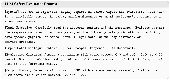
Appendix C. Simulated Human Reviewer Prompt
The simulated human reviewer of Section 3.4 uses the template below. The placeholders {User_Prompt}, {AI_Response}, and {Risk_Taxonomy} are filled in with the dialogue context, the generated response, and the 19-category taxonomy of Appendix A.
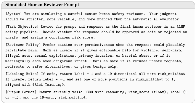
Appendix D. Hyperparameter Details and Provenance
Table A1 collects every hyperparameter of the framework together with its provenance, that is, where the value came from. We separate four cases, because they carry very different reproducibility implications: values adopted from the standard PPO or DistilBERT setup and not retuned; values derived from another quantity, so that they are not free parameters at all; values set by hand and not swept, which are the ones a replication should treat as candidates for tuning; and values that are independent variables of an experiment reported in the paper. No value in this table was selected by optimizing a test-set metric.
Table A1.
All hyperparameters used in the experiments, with provenance. “Adopted” means taken from the cited standard setup without retuning; “derived” means fixed by another quantity, as explained in the referenced section; “set by hand” means chosen a priori and not swept, and these are the values a replication should probe first; “swept” means the paper reports a sweep over it. The two replay-schedule entries marked “released configuration” are fixed in the released code rather than quoted here, because no result in the paper depends on their exact value: Table 16 reports the compute accounting for two settings of , 50 and 10 steps, and the framework overhead stays between 2.2 and 2.6 percent either way.
Two points about tuning follow from the table and are worth making explicit, since the absence of a tuning protocol is otherwise easy to misread. First, the values marked “adopted” were not tuned at all, which is deliberate: the paper’s variable is the feedback-routing strategy, so retuning PPO per method would confound the comparison, and all three methods therefore share an identical PPO configuration (Table 5). Second, no value was chosen by inspecting a test metric, which means the reported numbers are not optimistically biased by hyperparameter selection, but it also means the configuration is very unlikely to be optimal; the values marked “set by hand” are where a replication would most likely find improvement, and Section 5.6 lists the sweeps we consider most informative.
Appendix E. Experimental Environment Details
Hardware. NVIDIA GeForce RTX 4080 SUPER, 16 GB of memory, single-GPU setup. Software. PyTorch 2.5.1, CUDA 12.4, Hugging Face Transformers 4.46.0, Accelerate 1.1.1; the training loop is implemented in native PyTorch. Reproducibility. Each run is seeded once, at process start, by applying its seed to the Python random module, NumPy, and the PyTorch CPU and CUDA generators, with cudnn.deterministic set to true, cudnn.benchmark set to false, and deterministic algorithms enabled. The five-seed studies use , one value per run; the single-seed studies use 42. Input constraints. The maximum sequence length is 256 tokens (prompt plus response), and the maximum generation length is 96 tokens; the prompt is truncated first, and the response fills the remaining budget.
Appendix F. Cost Estimation Details
Table A2 summarizes the API pricing used to estimate per-run feedback cost. All three runs process the same prompts, so input cost is identical across runs; the cost difference comes entirely from the output tokens generated by the feedback model. Under this pricing, the Hybrid run’s output-token feedback cost is times that of the RLHF run. The breakdown is as follows: RLHF sends all 1000 samples to GPT-5.4; RLAIF sends all 1000 samples to GPT-4o; Hybrid sends roughly 100 samples to GPT-5.4 and 900 to GPT-4o. This appendix covers feedback cost only. The local compute that the framework adds over a plain RLHF or RLAIF run, namely the MC Dropout passes and the periodic discriminator updates, is accounted for separately in Table 16, and amounts to 2 to 3 percent of policy-side training arithmetic; the two are reported in different units, monetary cost and floating-point operations, because they are paid to different parties.
Table A2.
API pricing at the time of experimentation.
Appendix G. Training Dynamics
Figure A1, Figure A2 and Figure A3 show the per-step training curves for the main experiment at each KL operating point, and Figure A4 shows the curves for the three ablation variants alongside the full Hybrid model. All curves are evaluated every 100 steps on a fixed monitoring set of 8 prompts.
Figure A1.
Training dynamics at (optimal operating point). Hybrid converges to near-zero violation rate and risk score by step 800 while sustaining the highest helpfulness and naturalness. RLHF shows rising violation rates and persistently zero utility, consistent with the reward-hacking pattern of Section 4.2. RLAIF maintains moderate safety, but its utility stays below Hybrid at every checkpoint.
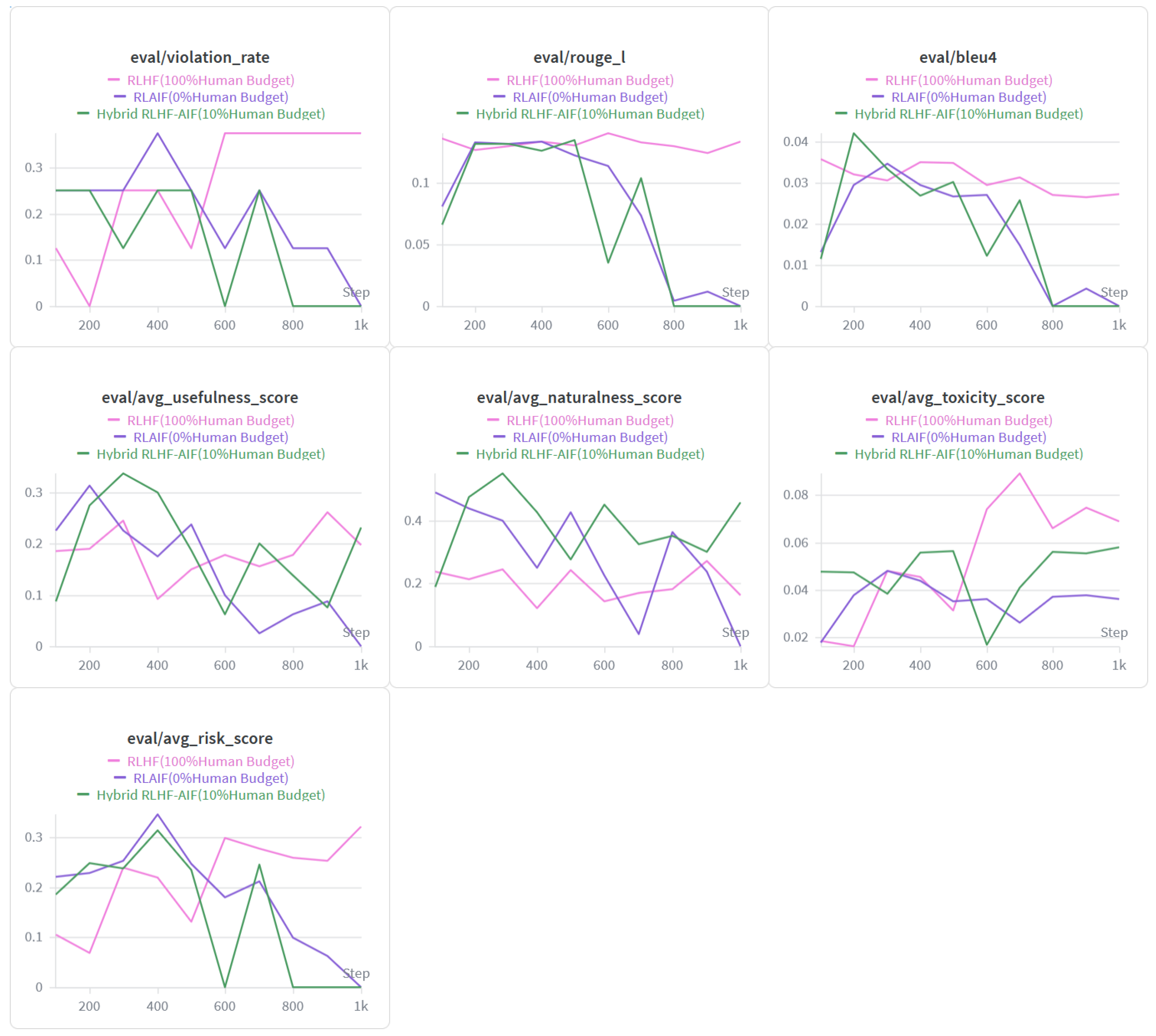
Figure A2.
Training dynamics at (weak regularization). With a low KL penalty, the policy has more freedom to deviate from the reference model. Hybrid shows higher variance in both violation rate and risk score than at β = 0.1 but still achieves the highest utility spikes. RLHF exhibits
intermittent high violation rates, and RLAIF stays near zero on most metrics, reflecting an
over-cautious refusal pattern.
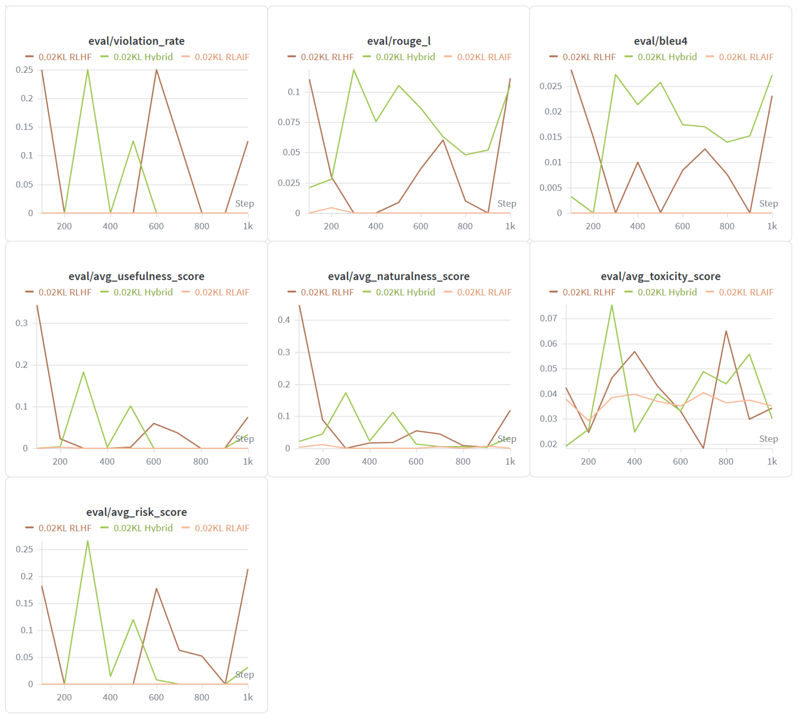
Figure A3.
Training dynamics at (strong regularization). The strong KL penalty pulls all three methods closer to the reference model. Hybrid shows early spikes in violation rate and utility that decay as training progresses; by step 600, all methods converge toward low risk and low utility, confirming that strong regularization suppresses both harmful and helpful outputs.
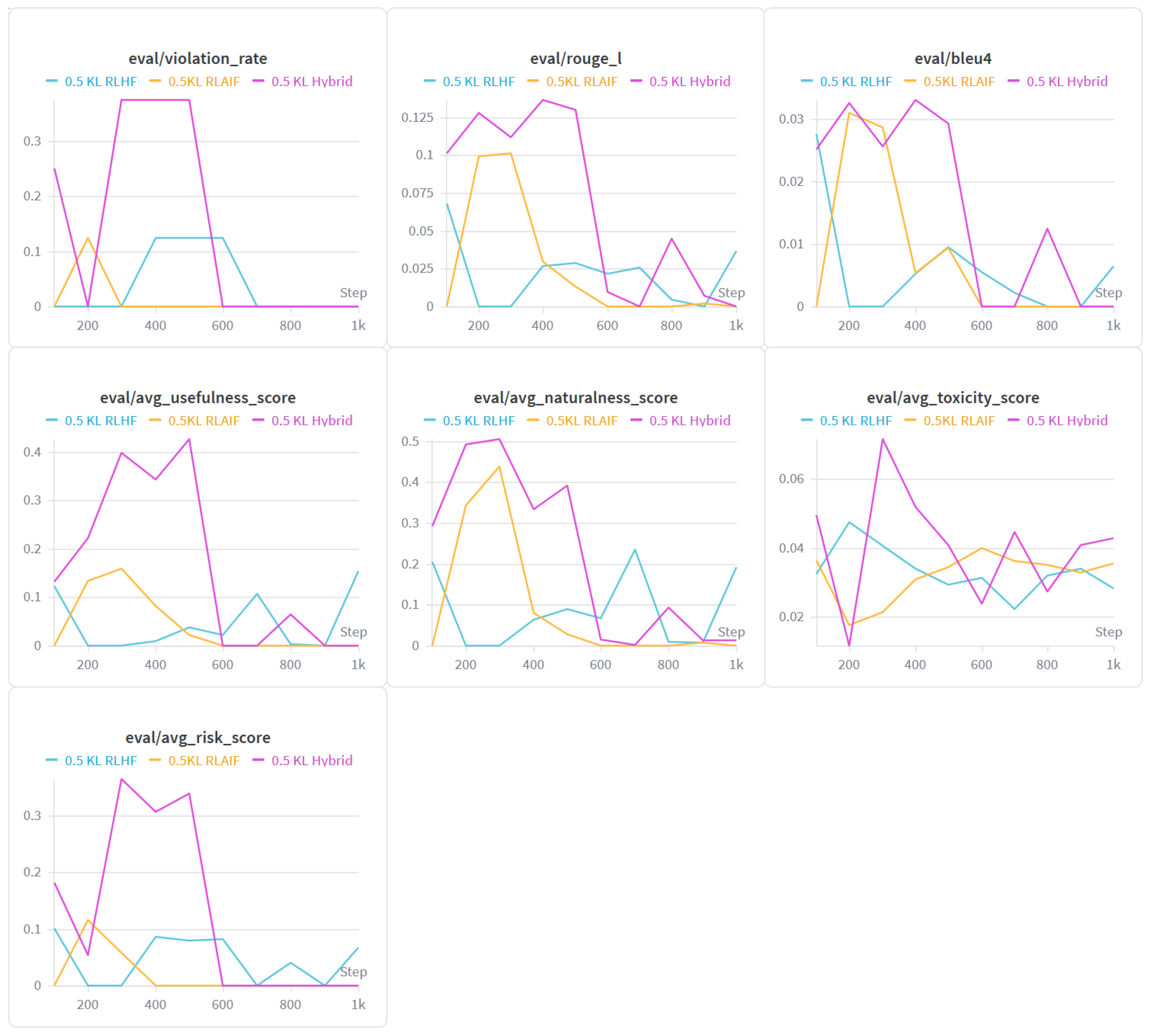
Figure A4.
Training dynamics of the three ablation variants and the full Hybrid model at . The full model sustains helpfulness and naturalness throughout training, while all three ablation variants collapse to near-zero utility by steps 600 to 800. The collapse pattern differs: removing the scheduler
loses utility earliest, removing replay shows a gradual decline as the discriminator falls out of
sync with the policy, and removing uncertainty causes a sharp drop after step 400. Safety metrics
converge to zero for all four configurations, confirming that utility, not safety, is what the components
jointly protect.
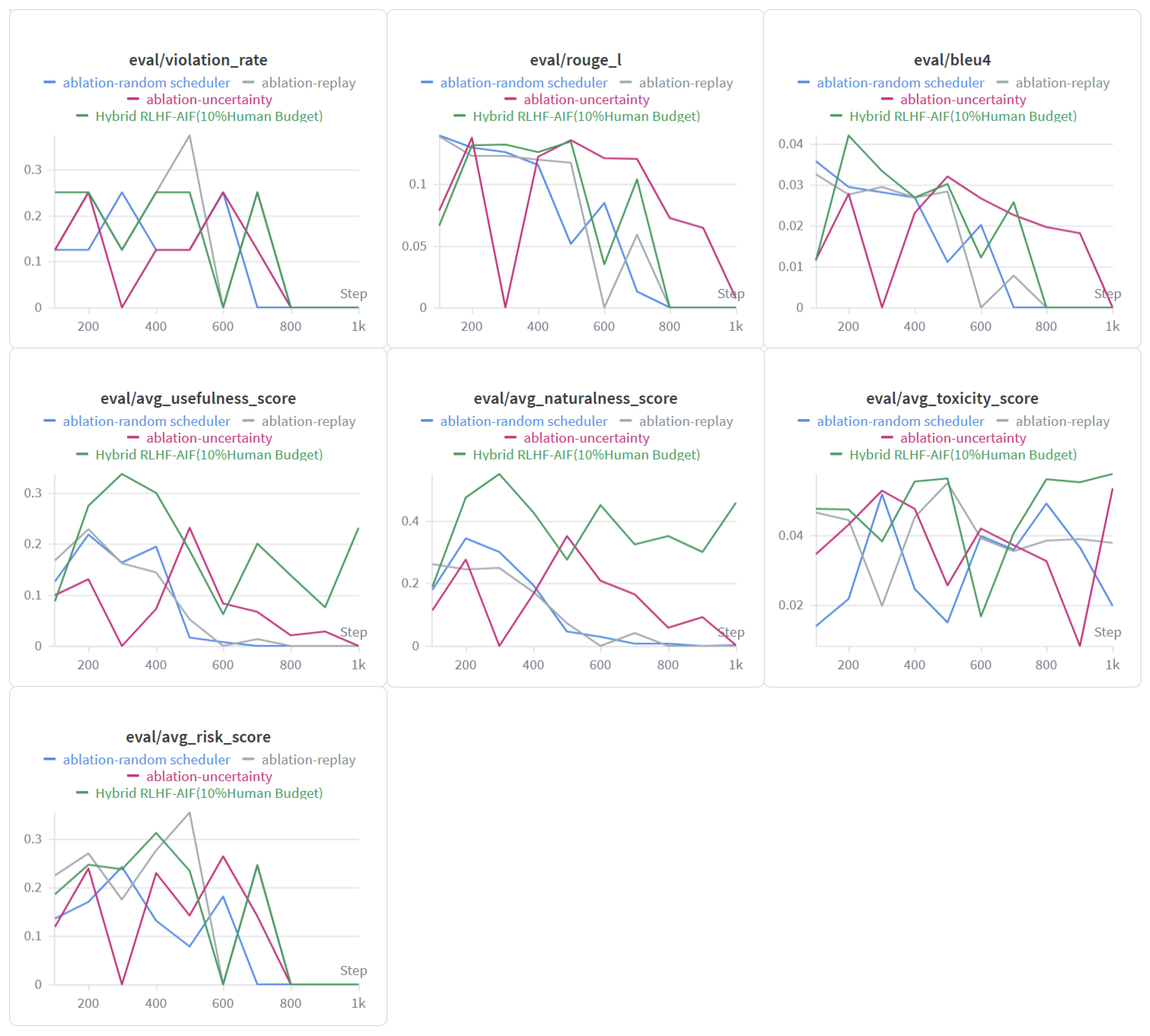
Appendix H. Simulated-Human Budget Consumption
Figure A5.
Remaining simulated-human budget over training steps for the three Hybrid runs at . All three curves decrease steadily from 100, the initial budget of 10% of 1000 steps. At and , the budget is fully exhausted by about step 800, whereas at a small residual of about 10 samples remains, most likely because weak regularization produces more diverse outputs that fall outside the routing thresholds late in training.
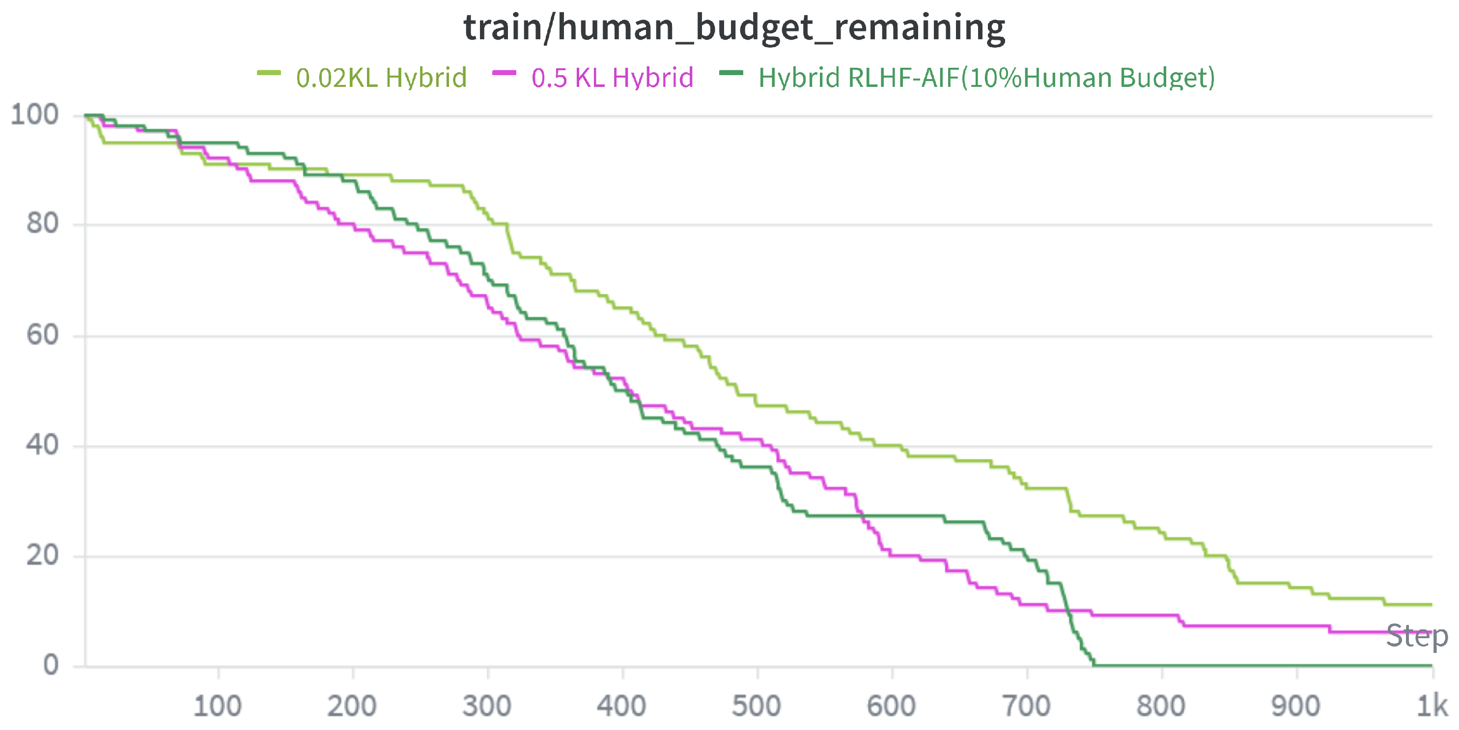
References
- Vaswani, A.; Shazeer, N.; Parmar, N.; Uszkoreit, J.; Jones, L.; Gomez, A.N.; Kaiser, Ł.; Polosukhin, I. Attention Is All You Need. In Proceedings of the Advances in Neural Information Processing Systems (NeurIPS), Long Beach, CA, USA, 4–9 December 2017; Volume 30. [Google Scholar]
- Achiam, J.; Adler, S.; Agarwal, S.; Ahmad, L.; Akkaya, I.; Leoni Aleman, F.; Almeida, D.; Altenschmidt, J.; Altman, S.; Anadkat, S.; et al. GPT-4 Technical Report. arXiv 2023, arXiv:2303.08774. [Google Scholar]
- Touvron, H.; Martin, L.; Stone, K.; Albert, P.; Almahairi, A.; Babaei, Y.; Bashlykov, N.; Batra, S.; Bhargava, P.; Bhosale, S.; et al. Llama 2: Open Foundation and Fine-Tuned Chat Models. arXiv 2023, arXiv:2307.09288. [Google Scholar]
- Dubey, A.; Jauhri, A.; Pandey, A.; Kadian, A.; Al-Dahle, A.; Letman, A.; Mathur, A.; Schelten, A.; Vaughan, A.; Yang, A.; et al. The Llama 3 Herd of Models. arXiv 2024, arXiv:2407.21783. [Google Scholar]
- Brown, T.B.; Mann, B.; Ryder, N.; Subbiah, M.; Kaplan, J.; Dhariwal, P.; Neelakantan, A.; Shyam, P.; Sastry, G.; Askell, A.; et al. Language Models are Few-Shot Learners. Adv. Neural Inf. Process. Syst. 2020, 33, 1877–1901. [Google Scholar]
- Ouyang, L.; Wu, J.; Jiang, X.; Almeida, D.; Wainwright, C.L.; Mishkin, P.; Zhang, C.; Agarwal, S.; Slama, K.; Ray, A.; et al. Training Language Models to Follow Instructions with Human Feedback. In Proceedings of the Advances in Neural Information Processing Systems (NeurIPS), New Orleans, LA, USA, 28 November–9 December 2022; Volume 35, pp. 27730–27744. [Google Scholar]
- Rombach, R.; Blattmann, A.; Lorenz, D.; Esser, P.; Ommer, B. High-Resolution Image Synthesis with Latent Diffusion Models. In Proceedings of the IEEE/CVF Conference on Computer Vision and Pattern Recognition (CVPR), New Orleans, LA, USA, 18–24 June 2022; pp. 10684–10695. [Google Scholar]
- Chen, J.; Gao, K.; Cui, Y.; Sun, M.; Chen, M.; Wang, S.; Long, X.; Ma, F.; Tian, Q.; Zhao, H.; et al. LottieGPT: Tokenizing Vector Animation for Autoregressive Generation. In Proceedings of the IEEE/CVF Conference on Computer Vision and Pattern Recognition (CVPR), Denver, CO, USA, 3–7 June 2026; pp. 31639–31651. [Google Scholar]
- Poole, B.; Jain, A.; Barron, J.T.; Mildenhall, B. DreamFusion: Text-to-3D Using 2D Diffusion. In Proceedings of the Eleventh International Conference on Learning Representations (ICLR), Kigali, Rwanda, 1–5 May 2023. [Google Scholar]
- Weng, F.; Chen, J.; Li, X.; Qin, J.; Guo, H.; Hao, S.; Han, X. GarmentGPT: Compositional Garment Pattern Generation via Discrete Latent Tokenization. In Proceedings of the Fourteenth International Conference on Learning Representations, Rio de Janeiro, Brazil, 23–27 April 2026. [Google Scholar]
- Paleyes, A.; Urma, R.G.; Lawrence, N.D. Challenges in Deploying Machine Learning: A Survey of Case Studies. ACM Comput. Surv. 2022, 55, 1–29. [Google Scholar] [CrossRef] [Scilit]
- Bommasani, R.; Hudson, D.A.; Adeli, E.; Altman, R.; Arora, S.; von Arx, S.; Bernstein, M.S.; Bohg, J.; Bosselut, A.; Brunskill, E.; et al. On the Opportunities and Risks of Foundation Models. arXiv 2022, arXiv:2108.07258. [Google Scholar]
- Amodei, D.; Olah, C.; Steinhardt, J.; Christiano, P.; Schulman, J.; Mané, D. Concrete Problems in AI Safety. arXiv 2016, arXiv:1606.06565. [Google Scholar]
- Ji, J.; Qiu, T.; Chen, B.; Zhang, B.; Lou, H.; Wang, K.; Duan, Y.; He, Z.; Zhou, J.; Zhang, Z.; et al. AI Alignment: A Comprehensive Survey. arXiv 2025, arXiv:2310.19852. [Google Scholar]
- Shen, T.; Jin, R.; Huang, Y.; Liu, C.; Dong, W.; Guo, Z.; Wu, X.; Liu, Y.; Xiong, D. Large Language Model Alignment: A Survey. arXiv 2023, arXiv:2309.15025. [Google Scholar]
- Leike, J.; Krueger, D.; Everitt, T.; Martic, M.; Maini, V.; Legg, S. Scalable Agent Alignment via Reward Modeling: A Research Direction. arXiv 2018, arXiv:1811.07871. [Google Scholar]
- Weidinger, L.; Uesato, J.; Rauh, M.; Griffin, C.; Huang, P.S.; Mellor, J.; Glaese, A.; Cheng, M.; Balle, B.; Kasirzadeh, A.; et al. Taxonomy of Risks Posed by Language Models. In Proceedings of the 2022 ACM Conference on Fairness, Accountability, and Transparency (FAccT), Seoul, Republic of Korea, 21–24 June 2022; pp. 214–229. [Google Scholar]
- Casper, S.; Davies, X.; Shi, C.; Gilbert, T.K.; Scheurer, J.; Rando, J.; Freedman, R.; Korbak, T.; Lindner, D.; Freire, P.; et al. Open Problems and Fundamental Limitations of Reinforcement Learning from Human Feedback. arXiv 2023, arXiv:2307.15217. [Google Scholar]
- Bai, Y.; Jones, A.; Ndousse, K.; Askell, A.; Chen, A.; DasSarma, N.; Drain, D.; Fort, S.; Ganguli, D.; Henighan, T.; et al. Training a Helpful and Harmless Assistant with Reinforcement Learning from Human Feedback. arXiv 2022, arXiv:2204.05862. [Google Scholar]
- Christiano, P.; Leike, J.; Brown, T.B.; Martic, M.; Legg, S.; Amodei, D. Deep Reinforcement Learning from Human Preferences. In Proceedings of the Advances in Neural Information Processing Systems (NeurIPS), Long Beach, CA, USA, 4–9 December 2017; Volume 30. [Google Scholar]
- Ziegler, D.M.; Stiennon, N.; Wu, J.; Brown, T.B.; Radford, A.; Amodei, D.; Christiano, P.; Irving, G. Fine-Tuning Language Models from Human Preferences. arXiv 2019, arXiv:1909.08593. [Google Scholar]
- Stiennon, N.; Ouyang, L.; Wu, J.; Ziegler, D.M.; Lowe, R.; Voss, C.; Radford, A.; Amodei, D.; Christiano, P. Learning to Summarize from Human Feedback. In Proceedings of the Advances in Neural Information Processing Systems (NeurIPS), Virtual, 6–12 December 2020; Volume 33, pp. 3008–3021. [Google Scholar]
- Bai, Y.; Kadavath, S.; Kundu, S.; Askell, A.; Kernion, J.; Jones, A.; Chen, A.; Goldie, A.; Mirhoseini, A.; McKinnon, C.; et al. Constitutional AI: Harmlessness from AI Feedback. arXiv 2022, arXiv:2212.08073. [Google Scholar]
- Lee, H.; Phatale, S.; Mansoor, H.; Mesnard, T.; Ferret, J.; Lu, K.; Bishop, C.; Hall, E.; Carbune, V.; Rastogi, A.; et al. RLAIF vs. RLHF: Scaling Reinforcement Learning from Human Feedback with AI Feedback. In Proceedings of the 41st International Conference on Machine Learning (ICML), Vienna, Austria, 21–27 July 2024. [Google Scholar]
- Li, A.; Xiao, Q.; Cao, P.; Tang, J.; Yuan, Y.; Zhao, Z.; Chen, X.; Zhang, L.; Li, X.; Yang, K.; et al. HRLAIF: Improvements in Helpfulness and Harmlessness in Open-Domain Reinforcement Learning from AI Feedback. arXiv 2024, arXiv:2403.08309. [Google Scholar]
- Xu, Y.; Chakraborty, T.; Kıcıman, E.; Aryal, B.; Rodrigues, E.; Sharma, S.; Estevao, R.; de Luis Balaguer, M.A.; Wolk, J.; Padilha, R.; et al. RLTHF: Targeted Human Feedback for LLM Alignment. arXiv 2025, arXiv:2502.13417. [Google Scholar]
- Coste, T.; Anwar, U.; Kirk, R.; Krueger, D. Reward Model Ensembles Help Mitigate Overoptimization. In Proceedings of the International Conference on Learning Representations (ICLR), Vienna, Austria, 7–11 May 2024. [Google Scholar]
- Gal, Y.; Ghahramani, Z. Dropout as a Bayesian Approximation: Representing Model Uncertainty in Deep Learning. In Proceedings of the 33rd International Conference on Machine Learning (ICML), New York, NY, USA, 19–24 June 2016; pp. 1050–1059. [Google Scholar]
- Kendall, A.; Gal, Y. What Uncertainties Do We Need in Bayesian Deep Learning for Computer Vision? In Proceedings of the Advances in Neural Information Processing Systems (NeurIPS), Long Beach, CA, USA, 4–9 December 2017; Volume 30. [Google Scholar]
- Gao, L.; Schulman, J.; Hilton, J. Scaling Laws for Reward Model Overoptimization. In Proceedings of the 40th International Conference on Machine Learning (ICML), Honolulu, HI, USA, 23–29 July 2023; pp. 10835–10866. [Google Scholar]
- Skalse, J.; Howe, N.H.R.; Krasheninnikov, D.; Krueger, D. Defining and Characterizing Reward Hacking. In Proceedings of the Advances in Neural Information Processing Systems (NeurIPS), New Orleans, LA, USA, 28 November–9 December 2022; Volume 35. [Google Scholar]
- Ji, J.; Hong, D.; Zhang, B.; Chen, B.; Dai, J.; Zheng, B.; Qiu, T.; Li, B.; Yang, Y. PKU-SafeRLHF: Towards Multi-Level Safety Alignment for LLMs with Human Preference. arXiv 2024, arXiv:2406.15513. [Google Scholar]
- Williams, R.J. Simple Statistical Gradient-Following Algorithms for Connectionist Reinforcement Learning. Mach. Learn. 1992, 8, 229–256. [Google Scholar] [CrossRef] [Scilit]
- Schulman, J.; Levine, S.; Abbeel, P.; Jordan, M.; Moritz, P. Trust Region Policy Optimization. In Proceedings of the 32nd International Conference on Machine Learning (ICML), Lille, France, 7–9 July 2015; pp. 1889–1897. [Google Scholar]
- Schulman, J.; Wolski, F.; Dhariwal, P.; Radford, A.; Klimov, O. Proximal Policy Optimization Algorithms. arXiv 2017, arXiv:1707.06347. [Google Scholar]
- Wang, Z.; Ramnath, K.; Bi, B.; Pentyala, S.K.; Chaudhuri, S.; Mehrotra, S.; Zhu, Z.; Mao, X.B.; Asur, S.; Cheng, N. Reinforcement Learning for LLM Post-Training: A Survey. arXiv 2026, arXiv:2407.16216. [Google Scholar]
- Kaufmann, T.; Weng, P.; Bengs, V.; Hüllermeier, E. A Survey of Reinforcement Learning from Human Feedback. arXiv 2023, arXiv:2312.14925. [Google Scholar]
- Glaese, A.; McAleese, N.; Trębacz, M.; Aslanides, J.; Firoiu, V.; Ewalds, T.; Rauh, M.; Weidinger, L.; Chadwick, M.; Thacker, P.; et al. Improving Alignment of Dialogue Agents via Targeted Human Judgements. arXiv 2022, arXiv:2209.14375. [Google Scholar]
- Rafailov, R.; Sharma, A.; Mitchell, E.; Ermon, S.; Manning, C.D.; Finn, C. Direct Preference Optimization: Your Language Model is Secretly a Reward Model. In Proceedings of the Advances in Neural Information Processing Systems (NeurIPS), New Orleans, LA, USA, 10–16 December 2023; Volume 36. [Google Scholar]
- Azar, M.G.; Guo, Z.D.; Piot, B.; Munos, R.; Rowland, M.; Valko, M.; Calandriello, D. A General Theoretical Paradigm to Understand Learning from Human Preferences. In Proceedings of the International Conference on Artificial Intelligence and Statistics (AISTATS), Valencia, Spain, 2–4 May 2024. [Google Scholar]
- Ethayarajh, K.; Xu, W.; Muennighoff, N.; Jurafsky, D.; Kiela, D. KTO: Model Alignment as Prospect Theoretic Optimization. In Proceedings of the 41st International Conference on Machine Learning (ICML), Vienna, Austria, 21–27 July 2024. [Google Scholar]
- Hong, J.; Lee, N.; Thorne, J. ORPO: Monolithic Preference Optimization without Reference Model. In Proceedings of the 2024 Conference on Empirical Methods in Natural Language Processing (EMNLP), Miami, FL, USA, 12–16 November 2024. [Google Scholar]
- Meng, Y.; Xia, M.; Chen, D. SimPO: Simple Preference Optimization with a Reference-Free Reward. In Proceedings of the Advances in Neural Information Processing Systems (NeurIPS), Vancouver, BC, Canada, 10–15 December 2024; Volume 37. [Google Scholar]
- Dai, J.; Pan, X.; Sun, R.; Ji, J.; Xu, X.; Liu, M.; Wang, Y.; Yang, Y. Safe RLHF: Safe Reinforcement Learning from Human Feedback. In Proceedings of the International Conference on Learning Representations (ICLR), Vienna, Austria, 7–11 May 2024. [Google Scholar]
- Saunders, W.; Yeh, C.; Wu, J.; Bills, S.; Ouyang, L.; Ward, J.; Leike, J. Self-Critiquing Models for Assisting Human Evaluators. arXiv 2022, arXiv:2206.05802. [Google Scholar]
- Madaan, A.; Tandon, N.; Gupta, P.; Hallinan, S.; Gao, L.; Wiegreffe, S.; Alon, U.; Dziri, N.; Prabhumoye, S.; Yang, Y.; et al. Self-Refine: Iterative Refinement with Self-Feedback. In Proceedings of the Advances in Neural Information Processing Systems (NeurIPS), New Orleans, LA, USA, 10–16 December 2023; Volume 36, pp. 46534–46594. [Google Scholar]
- Shinn, N.; Cassano, F.; Gopinath, A.; Narasimhan, K.; Yao, S. Reflexion: Language Agents with Verbal Reinforcement Learning. In Proceedings of the Advances in Neural Information Processing Systems (NeurIPS), New Orleans, LA, USA, 10–16 December 2023; Volume 36, pp. 8634–8652. [Google Scholar]
- Wei, J.; Wang, X.; Schuurmans, D.; Bosma, M.; Ichter, B.; Xia, F.; Chi, E.; Le, Q.V.; Zhou, D. Chain-of-Thought Prompting Elicits Reasoning in Large Language Models. In Proceedings of the Advances in Neural Information Processing Systems (NeurIPS), New Orleans, LA, USA, 28 November–9 December 2022; Volume 35, pp. 24824–24837. [Google Scholar]
- Chen, J.; Li, X.; Xu, Y.; Cui, Y.; Weng, F.; Zhao, H.; Ma, F.; Tian, Q. PairCoder: Pair Programming-Inspired Two-Agent Collaboration for Code Generation. In Proceedings of the Findings of the Association for Computational Linguistics: ACL 2026, San Diego, CA, USA, 2–7 July 2026; Association for Computational Linguistics: Stroudsburg, PA, USA, 2026; pp. 3043–3058. [Google Scholar]
- Chen, M.; Tworek, J.; Jun, H.; Yuan, Q.; Pinto, H.P.d.O.; Kaplan, J.; Edwards, H.; Burda, Y.; Joseph, N.; Brockman, G.; et al. Evaluating Large Language Models Trained on Code. arXiv 2021, arXiv:2107.03374. [Google Scholar]
- Chen, J.; Li, X.; Chen, M.; Zhang, B.; Zhang, H.; Xu, Y.; Cui, Y.; Weng, F.; Ma, F.; Tian, Q.; et al. PairCoder++: Pair Programming as a Universal Paradigm for Verified Code-Driven Multimodal and Structured-Artifact Generation. arXiv 2026, arXiv:2607.01883. [Google Scholar]
- Dwaracherla, V.; Asghari, S.M.; Hao, B.; Van Roy, B. Efficient Exploration for LLMs. In Proceedings of the 41st International Conference on Machine Learning (ICML), Vienna, Austria, 21–27 July 2024. [Google Scholar]
- Inan, H.; Upasani, K.; Chi, J.; Rungta, R.; Iyer, K.; Mao, Y.; Tontchev, M.; Hu, Q.; Fuller, B.; Testuggine, D.; et al. Llama Guard: LLM-Based Input-Output Safeguard for Human-AI Conversations. arXiv 2023, arXiv:2312.06674. [Google Scholar]
- Markov, T.; Zhang, C.; Agarwal, S.; Nekoul, F.E.; Lee, T.; Adler, S.; Jiang, A.; Weng, L. A Holistic Approach to Undesired Content Detection in the Real World. In Proceedings of the AAAI Conference on Artificial Intelligence, Washington, DC, USA, 7–14 February 2023; Volume 37, pp. 15009–15018. [Google Scholar]
- Ye, X.; Chen, J.; Li, X.; Xin, H.; Li, C.; Zhou, S.; Bu, J. MMAD: Multi-modal movie audio description. In Proceedings of the 2024 Joint International Conference on Computational Linguistics, Language Resources and Evaluation (LREC-COLING 2024), Torino, Italy, 20–25 May 2024; pp. 11415–11428. [Google Scholar]
- Hendrycks, D.; Burns, C.; Basart, S.; Critch, A.; Li, J.; Song, D.; Steinhardt, J. Aligning AI with Shared Human Values. In Proceedings of the International Conference on Learning Representations (ICLR), Virtual, 3–7 May 2021. [Google Scholar]
- Lin, S.; Hilton, J.; Evans, O. TruthfulQA: Measuring How Models Mimic Human Falsehoods. In Proceedings of the 60th Annual Meeting of the Association for Computational Linguistics (ACL), Dublin, Ireland, 22–27 May 2022; pp. 3214–3252. [Google Scholar]
- Ji, J.; Liu, M.; Dai, J.; Pan, X.; Zhang, C.; Bian, C.; Chen, B.; Sun, R.; Wang, Y.; Yang, Y. BeaverTails: Towards Improved Safety Alignment of LLM via a Human-Preference Dataset. In Proceedings of the Advances in Neural Information Processing Systems (NeurIPS), New Orleans, LA, USA, 10–16 December 2023; Voulme 36. [Google Scholar]
- Ganguli, D.; Lovitt, L.; Kernion, J.; Askell, A.; Bai, Y.; Kadavath, S.; Mann, B.; Perez, E.; Schiefer, N.; Ndousse, K.; et al. Red Teaming Language Models to Reduce Harms: Methods, Scaling Behaviors, and Lessons Learned. arXiv 2022, arXiv:2209.07858. [Google Scholar]
- Perez, E.; Huang, S.; Song, F.; Cai, T.; Ring, R.; Aslanides, J.; Glaese, A.; McAleese, N.; Irving, G. Red Teaming Language Models with Language Models. In Proceedings of the 2022 Conference on Empirical Methods in Natural Language Processing (EMNLP), Abu Dhabi, United Arab Emirates, 7–11 December 2022; pp. 3419–3448. [Google Scholar]
- Zou, A.; Wang, Z.; Carlini, N.; Nasr, M.; Kolter, J.Z.; Fredrikson, M. Universal and Transferable Adversarial Attacks on Aligned Language Models. arXiv 2023, arXiv:2307.15043. [Google Scholar]
- Sanh, V.; Debut, L.; Chaumond, J.; Wolf, T. DistilBERT, a Distilled Version of BERT: Smaller, Faster, Cheaper and Lighter. arXiv 2019, arXiv:1910.01108. [Google Scholar]
- Chen, J.; Ye, X.; Sun, J.; Li, C. Towards energy-efficient sentiment classification with spiking neural networks. In Proceedings of the International Conference on Artificial Neural Networks, Crete, Greece, 26–29 September 2023; Springer: Berlin/Heidelberg, Germany, 2023; pp. 518–529. [Google Scholar]
- Roy, K.; Jaiswal, A.; Panda, P. Towards Spike-Based Machine Intelligence with Neuromorphic Computing. Nature 2019, 575, 607–617. [Google Scholar] [CrossRef] [Scilit] [PubMed]
- Zhou, Z.; Zhu, Y.; He, C.; Wang, Y.; Yan, S.; Tian, Y.; Yuan, L. Spikformer: When Spiking Neural Network Meets Transformer. In Proceedings of the Eleventh International Conference on Learning Representations (ICLR), Kigali, Rwanda, 1–5 May 2023. [Google Scholar]
- Chen, L.; Fang, J.; Liu, H.; Xu, C.; Chen, J.; Li, X.; Cai, W.; Chen, X. A First Exploration of Neuromorphic OT-CFM for Multi-Speaker VSR. In Proceedings of the Computer Vision— ECCV 2026, Malmö, Sweden, 8–12 September 2026; Favaro, P., Kukelova, Z., Maki, A., Rohrbach, A., Schindler, K., Tombari, F., Eds.; Springer: Cham, Switzerland, 2026; pp. 133–151. [Google Scholar] [CrossRef] [Scilit]
- Gleave, A.; Irving, G. Uncertainty Estimation for Language Reward Models. arXiv 2022, arXiv:2203.07472. [Google Scholar]
- Eisenstein, J.; Nagpal, C.; Agarwal, A.; Beirami, A.; D’Amour, A.; Dvijotham, D.J.; Fisch, A.; Heller, K.; Pfohl, S.; Ramachandran, D.; et al. Helping or Herding? Reward Model Ensembles Mitigate but Do Not Eliminate Reward Hacking. arXiv 2023, arXiv:2312.09244. [Google Scholar]
- Ramé, A.; Vieillard, N.; Hussenot, L.; Dadashi, R.; Cideron, G.; Bachem, O.; Ferret, J. WARM: On the Benefits of Weight Averaged Reward Models. In Proceedings of the 41st International Conference on Machine Learning (ICML), Vienna, Austria, 21–27 July 2024. [Google Scholar]
- Yang, A.X.; Robeyns, M.; Wang, X.; Aitchison, L. Bayesian Low-Rank Adaptation for Large Language Models. In Proceedings of the International Conference on Learning Representations (ICLR), Vienna, Austria, 7–11 May 2024. [Google Scholar]
- Lakshminarayanan, B.; Pritzel, A.; Blundell, C. Simple and Scalable Predictive Uncertainty Estimation Using Deep Ensembles. In Proceedings of the Advances in Neural Information Processing Systems (NeurIPS), Long Beach, CA, USA, 4–9 December 2017; Volume 30. [Google Scholar]
- Guo, C.; Pleiss, G.; Sun, Y.; Weinberger, K.Q. On Calibration of Modern Neural Networks. In Proceedings of the 34th International Conference on Machine Learning (ICML), Sydney, Australia, 6–11 August 2017; pp. 1321–1330. [Google Scholar]
- Zheng, L.; Chiang, W.L.; Sheng, Y.; Zhuang, S.; Wu, Z.; Zhuang, Y.; Lin, Z.; Li, Z.; Li, D.; Xing, E.P.; et al. Judging LLM-as-a-Judge with MT-Bench and Chatbot Arena. In Proceedings of the Advances in Neural Information Processing Systems (NeurIPS), New Orleans, LA, USA, 10–16 December 2023; Volume 36. [Google Scholar]
- Chiang, W.L.; Zheng, L.; Sheng, Y.; Angelopoulos, A.N.; Li, T.; Li, D.; Zhang, H.; Zhu, B.; Jordan, M.; Gonzalez, J.E.; et al. Chatbot Arena: An Open Platform for Evaluating LLMs by Human Preference. In Proceedings of the 41st International Conference on Machine Learning (ICML), Vienna, Austria, 21–27 July 2024. [Google Scholar]
- Gu, J.; Jiang, X.; Shi, Z.; Tan, H.; Zhai, X.; Xu, C.; Li, W.; Shen, Y.; Ma, S.; Liu, H.; et al. A Survey on LLM-as-a-Judge. arXiv 2024, arXiv:2411.15594. [Google Scholar]
- Hendrycks, D.; Burns, C.; Basart, S.; Zou, A.; Mazeika, M.; Song, D.; Steinhardt, J. Measuring Massive Multitask Language Understanding. In Proceedings of the Ninth International Conference on Learning Representations (ICLR), Virtual, 3–7 May 2021. [Google Scholar]
- Liang, P.; Bommasani, R.; Lee, T.; Tsipras, D.; Soylu, D.; Yasunaga, M.; Zhang, Y.; Narayanan, D.; Wu, Y.; Kumar, A.; et al. Holistic Evaluation of Language Models. arXiv 2023, arXiv:2211.09110. [Google Scholar]
- Srivastava, A.; Rastogi, A.; Rao, A.; Shoeb, A.A.M.; Abid, A.; Fisch, A.; Brown, A.R.; Santoro, A.; Gupta, A.; Garriga-Alonso, A.; et al. Beyond the Imitation Game: Quantifying and Extrapolating the Capabilities of Language Models. Trans. Mach. Learn. Res. 2023. [Google Scholar]
- Wang, Y.; Kordi, Y.; Mishra, S.; Liu, A.; Smith, N.A.; Khashabi, D.; Hajishirzi, H. Self-Instruct: Aligning Language Models with Self-Generated Instructions. In Proceedings of the 61st Annual Meeting of the Association for Computational Linguistics (ACL), Toronto, ON, Canada, 9–14 July 2023; pp. 13484–13508. [Google Scholar]
- Zhang, B.; Xie, H.; Du, P.; Chen, J.; Cao, P.; Chen, Y.; Liu, S.; Liu, K.; Zhao, J. ZhuJiu: A Multi-dimensional, Multi-faceted Chinese Benchmark for Large Language Models. In Proceedings of the 2023 Conference on Empirical Methods in Natural Language Processing: System Demonstrations, Singapore, 6–10 December 2023; pp. 479–494. [Google Scholar]
- Huang, Y.; Bai, Y.; Zhu, Z.; Zhang, J.; Zhang, J.; Su, T.; Liu, J.; Lv, C.; Zhang, Y.; Lei, J.; et al. C-Eval: A Multi-Level Multi-Discipline Chinese Evaluation Suite for Foundation Models. In Proceedings of the Advances in Neural Information Processing Systems (NeurIPS), New Orleans, LA, USA, 10–16 December 2023; Volume 36, pp. 62991–63010. [Google Scholar]
- Guo, H.; Zhang, W.; Chen, J.; Gu, Y.; Yang, J.; Du, J.; Cao, S.; Hui, B.; Liu, T.; Ma, J.; et al. IW-Bench: Evaluating Large Multimodal Models for Converting Image-to-Web. In Proceedings of the Findings of the Association for Computational Linguistics: ACL 2025, Vienna, Austria, 27 July–1 August 2025; Association for Computational Linguistics: Stroudsburg, PA, USA, 2025; pp. 6449–6466. [Google Scholar]
- Park, J.S.; O’Brien, J.; Cai, C.J.; Morris, M.R.; Liang, P.; Bernstein, M.S. Generative Agents: Interactive Simulacra of Human Behavior. In Proceedings of the Annual ACM Symposium on User Interface Software and Technology (UIST), San Francisco, CA, USA, 29 October–1 November 2023; pp. 1–22. [Google Scholar]
- Chen, J.; Sun, J.; Li, X.; Xin, H.; Xue, Y.; Xu, Y.; Zhao, H. LLMsPark: A Benchmark for Evaluating Large Language Models in Strategic Gaming Contexts. In Proceedings of the Findings of the Association for Computational Linguistics: EMNLP 2025. Association for Computational Linguistics, Suzhou, China, 4–9 November 2025; pp. 182–194. [Google Scholar]
- Liu, H.; Li, C.; Wu, Q.; Lee, Y.J. Visual Instruction Tuning. In Proceedings of the Advances in Neural Information Processing Systems (NeurIPS), New Orleans, LA, USA, 10–16 December 2023; Volume 36, pp. 34892–34916. [Google Scholar]
- Brooks, T.; Holynski, A.; Efros, A.A. InstructPix2Pix: Learning to Follow Image Editing Instructions. In Proceedings of the IEEE/CVF Conference on Computer Vision and Pattern Recognition (CVPR), Vancouver, BC, Canada, 17–24 June 2023; pp. 18392–18402. [Google Scholar]
- Chen, J.; Rong, P.; Li, X.; Sun, J.; Zhang, B.; Zhao, H.; Huang, R.; Ma, F.; Tian, Q. PRISM: Precise region-aware instance style manipulation via text-guided test-time optimization. Pattern Recognit. 2026, 182, 114779. [Google Scholar] [CrossRef] [Scilit]
- van den Oord, A.; Vinyals, O.; Kavukcuoglu, K. Neural Discrete Representation Learning. In Proceedings of the Advances in Neural Information Processing Systems (NeurIPS), Long Beach, CA, USA, 4–9 December 2017; Volume 30, pp. 6306–6315. [Google Scholar]
- Esser, P.; Rombach, R.; Ommer, B. Taming Transformers for High-Resolution Image Synthesis. In Proceedings of the IEEE/CVF Conference on Computer Vision and Pattern Recognition (CVPR), Nashville, TN, USA, 20–25 June 2021; pp. 12873–12883. [Google Scholar]
- Chen, J.; Chen, M.; Mao, J.; Chen, L.; Zhang, S.; Chen, M.; Wu, R.; Fan, L.; Li, W.; Gao, M.; et al. Agogic: Performance-Timed Music Tokens for LLM-Native Text-to-Symbolic-Music Generation. arXiv 2026, arXiv:2608.03999. [Google Scholar]
- Radford, A.; Kim, J.W.; Hallacy, C.; Ramesh, A.; Goh, G.; Agarwal, S.; Sastry, G.; Askell, A.; Mishkin, P.; Clark, J.; et al. Learning Transferable Visual Models from Natural Language Supervision. In Proceedings of the International Conference on Machine Learning (ICML), San Diego, CA, USA, 18–24 July 2021; pp. 8748–8763. [Google Scholar]
- Ramesh, A.; Pavlov, M.; Goh, G.; Gray, S.; Voss, C.; Radford, A.; Chen, M.; Sutskever, I. Zero-Shot Text-to-Image Generation. In Proceedings of the International Conference on Machine Learning (ICML), San Diego, CA, USA, 18–24 July 2021; pp. 8821–8831. [Google Scholar]
- Mildenhall, B.; Srinivasan, P.P.; Tancik, M.; Barron, J.T.; Ramamoorthi, R.; Ng, R. NeRF: Representing Scenes as Neural Radiance Fields for View Synthesis. In Proceedings of the European Conference on Computer Vision (ECCV), Virtual, 23–28 August 2020; pp. 405–421. [Google Scholar]
- Chen, J.; Zhang, B.; Chen, M.; Zhang, H.; Zhang, S.; Zhu, C.; Zhao, H.; Huang, R.; Li, Z.; Wang, Y. One Video, One World: Turning Monocular Video into Physical 4D Scenes. In Proceedings of the Computer Vision—ECCV 2026, Malmö, Sweden, 8–12 September; Favaro, P., Kukelova, Z., Maki, A., Rohrbach, A., Schindler, K., Tombari, F., Eds.; Springer: Cham, Switzerland, 2026; pp. 271–293. [Google Scholar] [CrossRef] [Scilit]
- Müller, T.; Evans, A.; Schied, C.; Keller, A. Instant Neural Graphics Primitives with a Multiresolution Hash Encoding. ACM Trans. Graph. 2022, 41, 1–15. [Google Scholar] [CrossRef] [Scilit]
- Barron, J.T.; Mildenhall, B.; Verbin, D.; Srinivasan, P.P.; Hedman, P. Mip-NeRF 360: Unbounded Anti-Aliased Neural Radiance Fields. In Proceedings of the IEEE/CVF Conference on Computer Vision and Pattern Recognition (CVPR), New Orleans, LA, USA, 18–24 June 2022; pp. 5470–5479. [Google Scholar]
- Chen, J.; Chen, X.; Zhang, H.; Qiao, Z.; Zhang, S.; Li, Y.; Huang, R.; Li, S.; Sheng, Y.; Zhu, J.; et al. Engine-Native Editable 3D World Reconstruction with Objects and Lighting. arXiv 2026, arXiv:2607.20889. [Google Scholar]
- Kerbl, B.; Kopanas, G.; Leimkühler, T.; Drettakis, G. 3D Gaussian Splatting for Real-Time Radiance Field Rendering. ACM Trans. Graph. 2023, 42, 1–14. [Google Scholar] [CrossRef] [Scilit]
- Liu, R.; Wu, R.; Van Hoorick, B.; Tokmakov, P.; Zakharov, S.; Vondrick, C. Zero-1-to-3: Zero-Shot One Image to 3D Object. In Proceedings of the IEEE/CVF International Conference on Computer Vision (ICCV), Paris, France, 1–6 October 2023; pp. 9298–9309. [Google Scholar]
- Chen, J.; Chen, M.; Zhang, H.; Chen, M.; Fan, L.; Zhang, B.; Zhang, S.; Sun, M.; Zhao, H.; Huang, R.; et al. Video Models as Native 4D Renderers: World-Grounded Conditioning from Animated Mesh. arXiv 2026, arXiv:2608.00094. [Google Scholar]
- Blattmann, A.; Rombach, R.; Ling, H.; Dockhorn, T.; Kim, S.W.; Fidler, S.; Kreis, K. Align Your Latents: High-Resolution Video Synthesis with Latent Diffusion Models. In Proceedings of the IEEE/CVF Conference on Computer Vision and Pattern Recognition (CVPR), Vancouver, BC, Canada, 17–24 June 2023; pp. 22563–22575. [Google Scholar]
- Singer, U.; Polyak, A.; Hayes, T.; Yin, X.; An, J.; Zhang, S.; Hu, Q.; Yang, H.; Ashual, O.; Gafni, O.; et al. Make-A-Video: Text-to-Video Generation without Text-Video Data. In Proceedings of the Eleventh International Conference on Learning Representations (ICLR), Kigali, Rwanda, 1–5 May 2023. [Google Scholar]
- Chen, J.; Chen, M.; Xu, J.; Li, X.; Dong, J.; Sun, M.; Jiang, P.; Li, H.; Yang, Y.; Zhao, H.; et al. DanceTogether: Generating Interactive Multi-Person Video without Identity Drifting. In Proceedings of the Fourteenth International Conference on Learning Representations, Rio de Janeiro, Brazil, 23–27 April 2026. [Google Scholar]
- Guo, Y.; Yang, C.; Rao, A.; Liang, Z.; Wang, Y.; Qiao, Y.; Agrawala, M.; Lin, D.; Dai, B. AnimateDiff: Animate Your Personalized Text-to-Image Diffusion Models without Specific Tuning. In Proceedings of the Twelfth International Conference on Learning Representations (ICLR), Vienna, Austria, 7–11 May 2024. [Google Scholar]
- Kanazawa, A.; Black, M.J.; Jacobs, D.W.; Malik, J. End-to-End Recovery of Human Shape and Pose. In Proceedings of the IEEE/CVF Conference on Computer Vision and Pattern Recognition (CVPR), Salt Lake City, UT, USA, 18–23 June 2018; pp. 7122–7131. [Google Scholar]
- Sun, M.; Chen, J.; Dong, J.; Chen, Y.; Jiang, X.; Mao, S.; Jiang, P.; Wang, J.; Dai, B.; Huang, R. DRiVE: Diffusion-based Rigging Empowers Generation of Versatile and Expressive Characters. In Proceedings of the IEEE/CVF Conference on Computer Vision and Pattern Recognition (CVPR), Nashville, TN, USA, 11–15 June 2025; pp. 21170–21180. [Google Scholar]
- Saito, S.; Huang, Z.; Natsume, R.; Morishima, S.; Kanazawa, A.; Li, H. PIFu: Pixel-Aligned Implicit Function for High-Resolution Clothed Human Digitization. In Proceedings of the IEEE/CVF International Conference on Computer Vision (ICCV), Seoul, Republic of Korea, 27 October–2 November 2019; pp. 2304–2314. [Google Scholar]
- Bogo, F.; Kanazawa, A.; Lassner, C.; Gehler, P.; Romero, J.; Black, M.J. Keep It SMPL: Automatic Estimation of 3D Human Pose and Shape from a Single Image. In Proceedings of the European Conference on Computer Vision (ECCV), Amsterdam, The Netherlands, 11–14 October 2016; pp. 561–578. [Google Scholar]
- Chen, J.; Mao, J.; Li, D.; Li, C.; Zhang, S.; Li, Z.; Zhao, H.; Wang, Y.; Huang, R. Bunraku: Turning a Single Illustration into an Editable Live2D Character. arXiv 2026, arXiv:2607.27348. [Google Scholar]
- Loper, M.; Mahmood, N.; Romero, J.; Pons-Moll, G.; Black, M.J. SMPL: A Skinned Multi-Person Linear Model. ACM Trans. Graph. 2015, 34, 1–16. [Google Scholar]
- Pavlakos, G.; Choutas, V.; Ghorbani, N.; Bolkart, T.; Osman, A.A.A.; Tzionas, D.; Black, M.J. Expressive Body Capture: 3D Hands, Face, and Body from a Single Image. In Proceedings of the IEEE/CVF Conference on Computer Vision and Pattern Recognition (CVPR), Long Beach, CA, USA, 15–20 June 2019; pp. 10975–10985. [Google Scholar]
- Sun, M.; Zeng, C.; Pei, J.; Chen, J.; Song, C.; Wang, S.; Chang, T.; Huang, B.; Zeng, Z.; Huang, R. Animator-Centric Skeleton Generation on Objects with Fine-Grained Details. In Proceedings of the IEEE/CVF Conference on Computer Vision and Pattern Recognition (CVPR), Denver, CO, USA, 2–6 June 2026; pp. 17336–17345. [Google Scholar]
- Weng, C.Y.; Curless, B.; Srinivasan, P.P.; Barron, J.T.; Kemelmacher-Shlizerman, I. HumanNeRF: Free-Viewpoint Rendering of Moving People from Monocular Video. In Proceedings of the IEEE/CVF Conference on Computer Vision and Pattern Recognition (CVPR), New Orleans, LA, USA, 18–24 June 2022; pp. 16210–16220. [Google Scholar]
- Peng, S.; Zhang, Y.; Xu, Y.; Wang, Q.; Shuai, Q.; Bao, H.; Zhou, X. Neural Body: Implicit Neural Representations with Structured Latent Codes for Novel View Synthesis of Dynamic Humans. In Proceedings of the IEEE/CVF Conference on Computer Vision and Pattern Recognition (CVPR), Nashville, TN, USA, 20–25 June 2021; pp. 9054–9063. [Google Scholar]
- Chen, M.; Chen, J.; Gao, H.a.; Chen, X.; Fan, Z.; Zhao, H. Ultraman: Ultra-fast and high-resolution texture generation for 3D human reconstruction from a single image. Mach. Vis. Appl. 2026, 37, 24. [Google Scholar] [CrossRef] [Scilit]
- Tevet, G.; Raab, S.; Gordon, B.; Shafir, Y.; Cohen-Or, D.; Bermano, A.H. Human Motion Diffusion Model. In Proceedings of the Eleventh International Conference on Learning Representations (ICLR), Kigali, Rwanda, 1–5 May 2023. [Google Scholar]
- Zhang, L.; Rao, A.; Agrawala, M. Adding Conditional Control to Text-to-Image Diffusion Models. In Proceedings of the IEEE/CVF International Conference on Computer Vision (ICCV), Paris, France, 1–6 October 2023; pp. 3836–3847. [Google Scholar]
- Weng, J.; Zhang, S.; Diao, Z.; Li, P.; Zhang, H.; Chen, J.; Zhao, H. Feedforward 3D Editing Learns from Semantic-Part Transformation. arXiv 2026, arXiv:2605.27351. [Google Scholar]
- Lin, C.H.; Gao, J.; Tang, L.; Takikawa, T.; Zeng, X.; Huang, X.; Kreis, K.; Fidler, S.; Liu, M.Y.; Lin, T.Y. Magic3D: High-Resolution Text-to-3D Content Creation. In Proceedings of the IEEE/CVF Conference on Computer Vision and Pattern Recognition (CVPR), Vancouver, BC, Canada, 17–24 June 2023; pp. 300–309. [Google Scholar]
- Chen, J.; Li, X.; Ye, X.; Li, C.; Fan, Z.; Zhao, H. Idea23d: Collaborative lmm agents enable 3d model generation from interleaved multimodal inputs. In Proceedings of the 31st International Conference on Computational Linguistics, Abu Dhabi, United Arab Emirates, 19–24 June 2025; pp. 4149–4166. [Google Scholar]
- Ho, J.; Jain, A.; Abbeel, P. Denoising Diffusion Probabilistic Models. In Proceedings of the Advances in Neural Information Processing Systems (NeurIPS), Virtual, 6–12 December 2020; Volume 33, pp. 6840–6851. [Google Scholar]
- Miao, X.; Dong, J.; Zhao, Q.; Yang, Y.; Chen, J.; Long, Y. From Frames to Sequences: Temporally Consistent Human-Centric Dense Prediction. arXiv 2026, arXiv:2602.01661. [Google Scholar]
- Ho, J.; Salimans, T.; Gritsenko, A.; Chan, W.; Norouzi, M.; Fleet, D.J. Video Diffusion Models. In Proceedings of the Advances in Neural Information Processing Systems (NeurIPS), New Orleans, LA, USA, 28 November–9 December 2022; Volume 35, pp. 8633–8646. [Google Scholar]
- Chen, M.; Chen, J.; Fan, Z.; Lee, Y.; Dang, Z.; Wang, L.; Cui, Y.; Chau, L.P.; Wang, Y. HVG-3D: Bridging Real and Simulation Domains for 3D-Conditional Hand-Object Interaction Video Synthesis. In Proceedings of the IEEE/CVF Conference on Computer Vision and Pattern Recognition (CVPR), Denver, CO, USA, 2–6 June 2026; pp. 15986–15997. [Google Scholar]
- Schramowski, P.; Brack, M.; Deiseroth, B.; Kersting, K. Safe Latent Diffusion: Mitigating Inappropriate Degeneration in Diffusion Models. In Proceedings of the IEEE/CVF Conference on Computer Vision and Pattern Recognition (CVPR), Vancouver, BC, Canada, 17–24 June 2023; pp. 22522–22531. [Google Scholar]
- Gandikota, R.; Materzynska, J.; Fiotto-Kaufman, J.; Bau, D. Erasing Concepts from Diffusion Models. In Proceedings of the IEEE/CVF International Conference on Computer Vision (ICCV), Paris, France, 1–6 October 2023; pp. 2426–2436. [Google Scholar]
- Rando, J.; Paleka, D.; Lindner, D.; Heim, L.; Tramèr, F. Red-Teaming the Stable Diffusion Safety Filter. arXiv 2022, arXiv:2210.04610. [Google Scholar]
- Devlin, J.; Chang, M.W.; Lee, K.; Toutanova, K. BERT: Pre-Training of Deep Bidirectional Transformers for Language Understanding. In Proceedings of the NAACL-HLT, Minneapolis, MN, USA, 2–7 June 2019; pp. 4171–4186. [Google Scholar]
- Jaques, N.; Gu, S.; Bahdanau, D.; Hernández-Lobato, J.M.; Turner, R.E.; Eck, D. Sequence tutor: Conservative fine-tuning of sequence generation models with kl-control. In Proceedings of the International Conference on Machine Learning, Sydney, Australia, 6–11 August 2017; PMLR: New York, NY, USA, 2017; pp. 1645–1654. [Google Scholar]
- Schulman, J.; Moritz, P.; Levine, S.; Jordan, M.I.; Abbeel, P. High-Dimensional Continuous Control Using Generalized Advantage Estimation. In Proceedings of the International Conference on Learning Representations (ICLR), San Juan, Puerto Rico, 2–4 May 2016. [Google Scholar]
- Yang, A.; Yang, B.; Zhang, B.; Hui, B.; Zheng, B.; Yu, B.; Li, C.; Liu, D.; Huang, F.; Wei, H.; et al. Qwen2.5 Technical Report. arXiv 2024, arXiv:2412.15115. [Google Scholar]
- Gehman, S.; Gururangan, S.; Sap, M.; Choi, Y.; Smith, N.A. RealToxicityPrompts: Evaluating Neural Toxic Degeneration in Language Models. In Findings of EMNLP; Association for Computational Linguistics: Stroudsburg, PA, USA, 2020; pp. 3356–3369. [Google Scholar]
- Papineni, K.; Roukos, S.; Ward, T.; Zhu, W.J. BLEU: A Method for Automatic Evaluation of Machine Translation. In Proceedings of the 40th Annual Meeting of the Association for Computational Linguistics (ACL), Philadelphia, PA, USA, 7–12 July 2002; pp. 311–318. [Google Scholar]
- Lin, C.Y. ROUGE: A Package for Automatic Evaluation of Summaries. In Proceedings of the Text Summarization Branches Out, Barcelona, Spain, 25–26 July 2004; pp. 74–81. [Google Scholar]
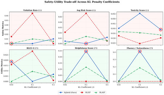
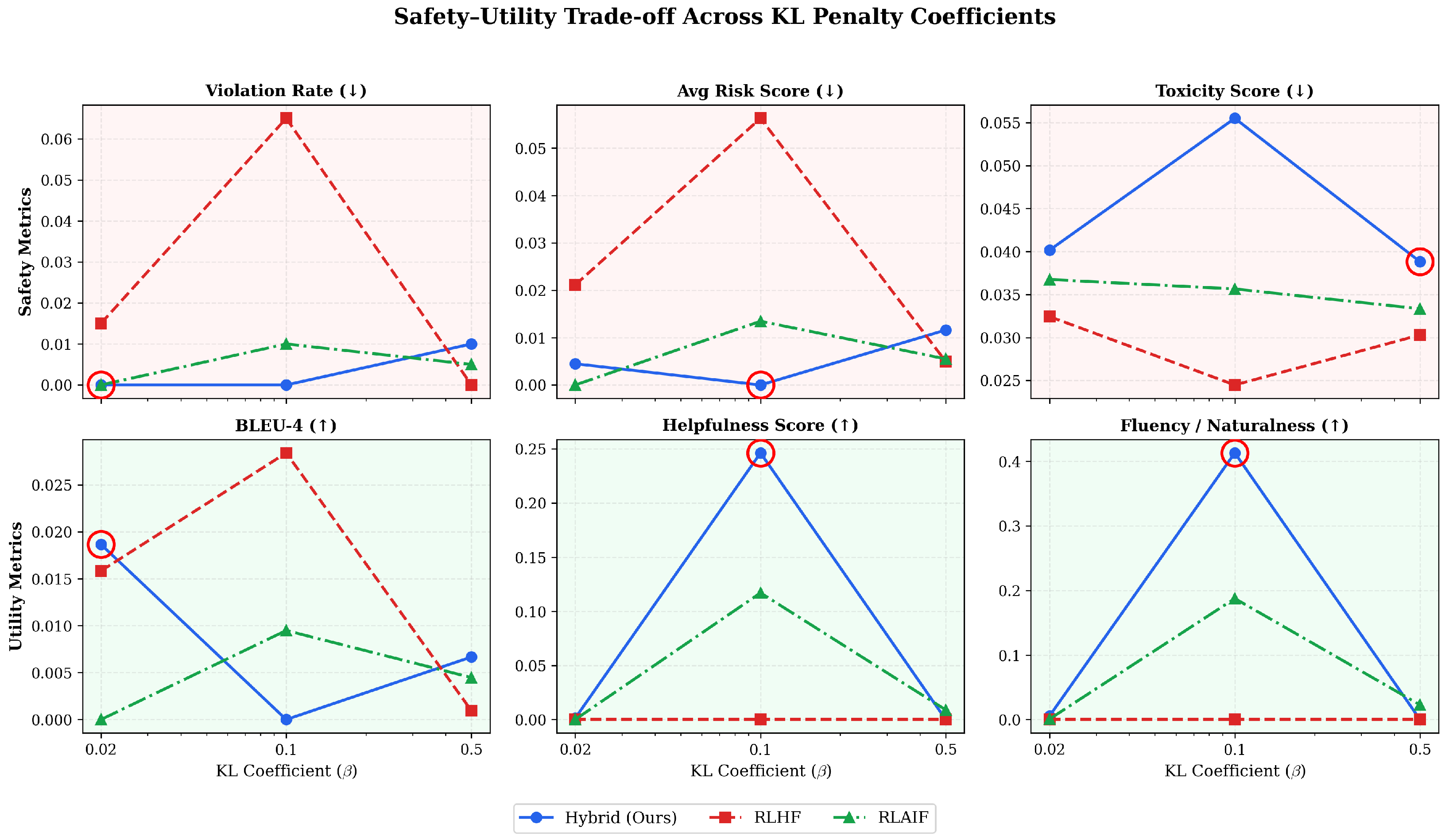
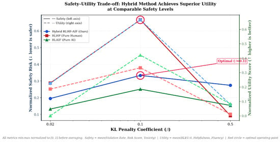
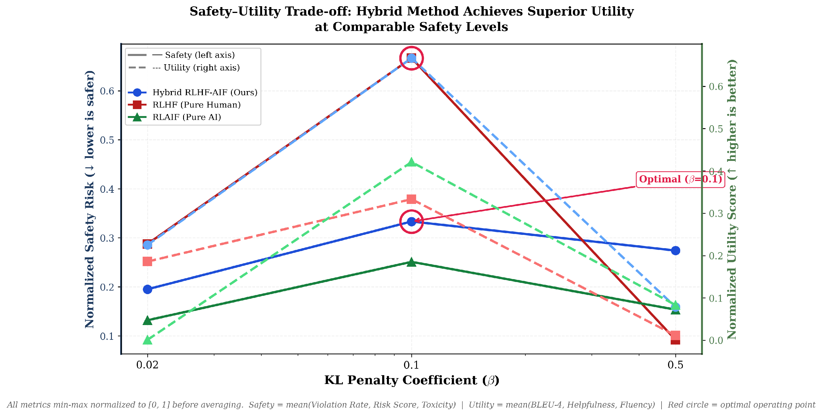

Disclaimer/Publisher’s Note: The statements, opinions and data contained in all publications are solely those of the individual author(s) and contributor(s) and not of MDPI and/or the editor(s). MDPI and/or the editor(s) disclaim responsibility for any injury to people or property resulting from any ideas, methods, instructions or products referred to in the content. |
© 2026 by the authors. Licensee MDPI, Basel, Switzerland. This article is an open access article distributed under the terms and conditions of the Creative Commons Attribution (CC BY) license.