


Abstract
This paper uses linear mean–variance preferences within the Markowitz mean–variance framework to characterize bidders’ trade-off between return and risk and extends first- and second-price sealed-bid auction models to risky environments. Compared with conventional models that maximize expected payoff or represent risk aversion through expected utility, this framework does not rely on a specific utility function, characterizes bidders’ risk attitudes more directly, and facilitates quantitative analysis of how those attitudes affect equilibrium bidding, optimal reserve prices, seller revenue, and social welfare under the adopted mean–variance criterion. We characterize the equilibrium bidding strategies, optimal reserve prices, and seller’s expected revenue in the two auction formats, together with their rankings; analyze the effects of bidders’ variance aversion and the number of bidders; and trace the new findings to bidders’ variance aversion. For social welfare, we quantify the welfare loss caused by mean–variance preferences, rank social welfare across auction formats and preference types, and show that the welfare-maximizing reserve price lies below the seller-optimal reserve price in each format. These results inform the choice of an appropriate reserve price in practice to reduce the welfare loss caused by bidders’ variance aversion. Finally, we briefly consider three extensions: an asymmetric model, exogenous shocks to bidders’ payoffs, and nonlinear mean–variance preferences.
Keywords:
mean–variance preferences; variance aversion; first-price sealed-bid auction; second-price sealed-bid auction; reserve price; seller revenue; social welfare MSC:
91B26; 91A27
1. Introduction
First- and second-price sealed-bid auctions have been widely used to model resource allocation mechanisms, such as government procurement processes, spectrum license allocations, and supply chain sourcing decisions. Bidder preferences are pivotal in determining the equilibrium bidding strategy in auctions. Traditional analyses of winner-pay auctions assume that risk-neutral bidders maximize their expected payoff [1,2,3]. However, many studies assume that bidders are risk-averse [4,5]—a characteristic that aligns with individuals’ aversion to uncertainty in practical economic activities such as investment decision-making. Empirical studies of timber and procurement auctions show that bidder risk aversion and its heterogeneity are empirically relevant [6,7,8]. Furthermore, risk-averse bidders submit more aggressive bids than risk-neutral bidders in first-price sealed-bid auctions [5,9]. Consequently, it is important to study sealed-bid auctions under different bidders’ preferences.
Recently, Klose and Schweinzer [10] have introduced a novel modeling perspective—mean–variance preferences—to formally characterize the objective function of variance-averse bidders in an all-pay auction. This provides a new way to characterize bidders’ risk attitudes. Following them, we model bidders’ risk attitudes using mean–variance preferences in the first- and second-price sealed-bid auctions. A bidder maximizes expected payoff minus the variance aversion parameter multiplied by payoff variance, so the parameter directly measures the degree of variance aversion. The criterion originates in Markowitz’s portfolio analysis [11] and was subsequently connected to expected utility and given choice-theoretic foundations [12,13,14,15]. Compared with the conventional expected utility representation of bidders’ risk attitudes, mean–variance preferences offer several advantages. First, expected utility represents risk aversion through a concave utility function, and different functional forms yield different equilibrium bids. Mean–variance preferences do not depend on a particular functional form; instead, they characterize bidders’ trade-off between return and risk through the intuitive measures of expected payoff and payoff variance. Second, a single variance aversion parameter represents different degrees of variance aversion, facilitating quantitative analysis of how bidders’ risk attitudes affect equilibrium bidding, seller revenue, and social welfare under the adopted mean–variance criterion. Third, the linear criterion expresses bidders’ mean–variance-adjusted payoffs in monetary units. Aggregating these payoffs with seller revenue using explicitly specified welfare weights provides a common monetary measure of mean–variance social welfare for comparing alternative allocations while accounting for payoff risk. Finally, as a decision criterion widely used in finance, mean–variance preferences provide an intuitive and simple basis for decision-making in real-world auction settings.
In our analysis, we first characterize equilibrium bidding. The unique symmetric equilibrium bidding strategy in the first-price sealed-bid auction satisfies an ordinary differential equation. Equilibrium bids increase with both the degree of bidders’ variance aversion and the number of bidders. In the second-price sealed-bid auction, truthful bidding remains optimal. Mean–variance preferences therefore reproduce the established bidding response to variance aversion in the first-price sealed-bid auction while preserving the allocation and payment incentives associated with truthful bidding in the second-price sealed-bid auction.
We then examine reserve prices, the seller’s expected revenue, and social welfare under an explicitly specified mean–variance criterion. The seller-optimal reserve price in the first-price sealed-bid auction is lower than that in the second-price sealed-bid auction and decreases with the degree of bidders’ variance aversion. The seller’s expected revenue is higher in the first-price sealed-bid auction than in the second-price sealed-bid auction, both at a fixed reserve price and after the reserve price is optimized in each format. The seller’s expected revenue in both formats also increases with the number of bidders. Under this mean–variance criterion, the first-price sealed-bid auction generates a smaller sum of bidders’ payoff variances and higher social welfare. The reserve price that maximizes social welfare lies between the seller’s reservation value and the seller-optimal reserve price in each auction format.
Finally, we consider three extensions. The first allows bidders to differ in their value distributions and variance aversion parameters. Any differentiable equilibrium in the first-price sealed-bid auction satisfies a system of inverse bid differential equations, while truthful bidding remains optimal in the second-price sealed-bid auction. The second extension introduces exogenous shocks to payoffs after winning and losing. At an interior equilibrium where the cutoff equation has positive slope, the locally unique cutoff root rises with the variance of either shock, and any nearby equilibrium in the same class must use that root. Among equilibria with a common participation cutoff, reallocating variance from the losing state to the winning state lowers equilibrium bids. The third extension derives bidding under a nonlinear marginal trade-off between the payoff mean and variance.
This paper makes four contributions. First, it enriches the literature on overbidding in the first-price sealed-bid auction [16,17] and bidding behavior in the second-price sealed-bid auction under risk aversion [18,19] by providing an explanation based on mean–variance preferences. Second, it extends the analysis of auctions under mean–variance preferences [10,20], moving beyond all-pay auctions to examine winner-pay auctions. Third, it contributes to the literature on bidder payoffs and seller revenue comparisons under risk aversion [9,19,21] by adding welfare calculations within the present mean–variance framework. Fourth, it extends the analysis to heterogeneous bidders [22,23,24] and post-bid or post-auction payoff uncertainty [25,26,27,28], deriving tractable necessary conditions for separating equilibria and conditional comparative statics. The analysis thus provides a unified mean–variance framework for equilibrium bidding, the reserve price, the seller’s expected revenue, and social welfare under the adopted mean–variance criterion across sealed-bid auction environments.
The remainder of the paper is organized as follows: Section 2 reviews the related literature. Section 3 presents the model. Section 4 characterizes equilibrium bidding. Section 5 studies optimal reserve prices and the seller’s expected revenue. Section 6 analyzes social welfare under the adopted mean–variance criterion. Section 7 presents numerical examples and a simulation of bidding incentives. Section 8 considers asymmetric bidders, exogenous payoff shocks, and nonlinear mean–variance preferences. Section 9 concludes. All proofs are collected in Appendix A.
2. Literature Review
Variance aversion under mean–variance preferences is analogous, but not identical, to risk aversion under expected utility. We review the related literature from three perspectives: risk aversion in sealed-bid auctions and its conventional representation, the effects of risk aversion, and the development of mean–variance preferences and their applications to auctions.
2.1. Risk Aversion in Sealed-Bid Auctions and Its Conventional Representation
Bidding in a sealed-bid auction is inherently a decision under uncertainty. A bidder chooses a bid without observing rivals’ valuations or bids, so both the probability of winning and the resulting monetary payoff are uncertain. Risk attitudes therefore enter directly into the trade-off between winning more often and retaining a larger surplus conditional on winning. Under symmetric independent private values and risk neutrality, truthful bidding is weakly dominant in the second-price sealed-bid auction, equilibrium bids in the first-price sealed-bid auction lie below values, and the two formats satisfy revenue equivalence [2,29,30]. These benchmark results isolate the strategic effects of the payment rule. Once bidders are risk-averse, the same allocation and payment rules generate different bidding incentives because bidders care about the distribution of monetary payoffs rather than only their expectation.
Expected utility theory provides the conventional framework for representing this behavior. A bidder evaluates the monetary payoff from each bid through an increasing and concave utility function. Risk neutrality corresponds to linear utility, whereas greater curvature represents a stronger aversion to payoff uncertainty. This formulation embeds risk attitudes directly in the bidder’s optimization problem and permits the equilibrium bid to be derived from the interaction between the auction rule, the distribution of rival values, and the curvature of utility. Because utility is defined over final wealth, background wealth and other sources of uncertainty may also affect the bidder’s response to auction risk. Related expected utility research shows, in particular, that random initial wealth can change attitudes toward risky payoffs [31].
The importance of risk aversion in auctions is supported by both experimental and structural evidence. Cox et al. [32] document a systematic relationship between risk aversion and bidding in first-price sealed-bid auctions. Füllbrunn et al. [16] revisit the extent to which risk attitudes account for bids above the risk-neutral benchmark, highlighting the continuing role of risk preferences in explaining observed bidding behavior. Structural and empirical auction studies recover bidders’ latent values, costs, or preference parameters from observed or experimental bid and entry data [6,7,8,17,33,34,35]. Because both valuations and risk attitudes are latent, identification often relies on observable variation in the competitive environment. Chen et al. [36], for example, show how changes in potential competition and entry costs can identify the underlying value, cost, and preference primitives. Risk aversion is consequently not only a theoretical departure from the risk-neutral benchmark but also an empirically relevant component of auction behavior.
2.2. Effects of Risk Aversion in Sealed-Bid Auctions
The most direct effect of risk aversion appears in equilibrium bidding. In a first-price sealed-bid auction, a higher bid raises the probability of winning but reduces the surplus retained when the bidder wins. A risk-averse bidder places greater value on increasing the probability of obtaining a positive payoff and is therefore willing to surrender part of the winning surplus. Equilibrium bids consequently rise relative to the risk-neutral benchmark [5,9]. The effect differs fundamentally in a second-price sealed-bid auction. A bidder’s own bid determines whether the object is won but does not determine the payment conditional on winning. As long as utility is increasing in monetary payoff, truthful bidding remains weakly dominant. Risk aversion therefore alters bidding directly in the first-price format while leaving the basic bidding rule in the second-price format unchanged.
Experimental findings are broadly consistent with this theoretical mechanism. Cox et al. [32] associate risk aversion with more aggressive first-price bidding, while Füllbrunn et al. [16] examine its contribution to the recurrent experimental finding that bids exceed the risk-neutral equilibrium. Structural and experimental estimation studies use bid behavior to infer preference parameters [6,7,8,17,33,34]. The estimated relationship between risk preferences and bids also depends on participation. When entry is costly, observed bids come from a selected group of bidders whose valuations and risk attitudes make participation worthwhile. The entry decision must therefore be considered together with the bidding decision when interpreting the effect of risk aversion [35,36].
The increase in first-price bids has immediate implications for the seller’s expected revenue. Since second-price bidding remains truthful while first-price bids become more aggressive, risk aversion can give the first-price sealed-bid auction a revenue advantage [5,9,19,37]. This ranking is driven by the payment rule rather than by a change in the efficient ordering of symmetric bidders: the first-price format induces bidders to insure themselves partly against losing by submitting higher bids, and the seller captures the resulting reduction in the winner’s surplus. Revenue equivalence, which holds under the standard risk-neutral assumptions, therefore need not survive when bidders are risk-averse.
The revenue comparison becomes less direct when participation is endogenous. A more aggressive bidding strategy affects the payoff from entering as well as the payment conditional on winning. Risk aversion may consequently change the number and composition of participants, and this extensive-margin response can offset the revenue effect generated by higher bids. Smith and Levin [21] show that endogenous entry may alter the ranking of auction formats, while Vasserman and Watt [19] discuss more generally how risk attitudes and participation interact in revenue comparisons. Seller revenue is thus determined by two related responses: risk aversion changes how entrants bid and whether potential bidders enter in the first place.
Risk aversion also changes the seller’s optimal reserve price. Under risk neutrality, the optimal reserve price balances the additional revenue obtained from excluding low-value bidders against the probability that the object remains unsold. The resulting condition equates the bidder’s virtual value to the seller’s reservation value [2,29]. With risk-averse bidders, a reserve price also affects the aggressiveness of equilibrium bidding among the remaining types. The seller’s exclusion decision and bidders’ risk responses must therefore be determined jointly.
Hu et al. [4] show that buyer risk aversion lowers the optimal reserve price in the first-price sealed-bid auction but leaves the reserve price condition in the second-price sealed-bid auction unchanged. The distinction mirrors the effect of risk aversion on bidding: a first-price reserve changes an equilibrium in which risk preferences already influence bids, whereas truthful bidding preserves the standard second-price condition. Hu [38] further shows that the optimal first-price reserve price decreases with the number of bidders under buyer or seller risk aversion. Increased competition and risk-induced bidding both raise payments, reducing the seller’s reliance on exclusion as a source of revenue. Related work under reference-dependent preferences also produces format-specific reserve price conditions, illustrating the broader sensitivity of optimal reserves to bidders’ evaluation of risky outcomes [39].
The consequences of risk aversion extend beyond equilibrium bidding to bidder utility and auction-format revenue or procurement cost comparisons [5,9,19,21,37,40]. We therefore analyze allocative surplus and social welfare under the adopted mean–variance criterion separately. Higher first-price bids reduce the monetary surplus retained by the winner, even when they increase the bidder’s probability of winning. A revenue gain for the seller therefore does not by itself establish a welfare improvement.
In a symmetric auction with monotone bidding and no entry distortion, the object continues to be allocated to the bidder with the highest value. Risk aversion may then change the distribution of monetary payoffs without changing the identity of the winner. Once reserve prices or endogenous entry are introduced, however, risk attitudes may also affect whether the object is sold and which bidders participate. Welfare comparisons must then account jointly for allocative surplus, entry costs, and the risk borne by bidders.
This distinction also appears in mechanism design research. Che and Gale [37] examine auction design under preferences that depart from the standard risk-neutral benchmark, while Gershkov et al. [41] study mechanisms that insure truthful types against payoff changes caused by other agents’ reports. Their analysis emphasizes that expected payments do not fully describe the consequences of a mechanism when agents care about payoff uncertainty. Auction formats can generate similar expected allocations or revenues while exposing bidders to different patterns of risk. The welfare effects of risk aversion therefore arise from both the allocation of the object and the allocation of uncertain payoffs across participants.
2.3. Development of Mean–Variance Preferences and Their Applications to Auctions
Mean–variance analysis offers an alternative way to represent attitudes toward risky payoffs. It originated in Markowitz’s portfolio theory, where an investment is evaluated through its expected return and the variance of that return [11]. The framework makes the central trade-off explicit: decision makers value a higher expected payoff but dislike greater dispersion around that expectation. Rather than describing risk attitudes through the curvature of a utility function over every possible wealth level, the mean–variance criterion summarizes a risky prospect through its first two moments.
Subsequent research established the decision-theoretic foundations of this representation. Levy and Markowitz [13] show that mean–variance approximations can closely track expected utility rankings for the return distributions and utility functions they study. Chiu [12], Nakamura [14], and Qu [15] provide direct choice-theoretic foundations for mean–variance preferences. These contributions place mean–variance analysis within the broader theory of choice under uncertainty rather than treating it solely as a computational device developed for portfolio selection.
Direct applications of mean–variance preferences in auction theory remain limited. Klose and Schweinzer [10] introduce mean–variance preferences into an all-pay auction, where every bidder pays regardless of whether the object is won. They show that the weight placed on payoff variance affects low- and high-value bidders differently. The result reflects the interaction between the all-pay payment rule and type-dependent winning probabilities: bidders at different parts of the value distribution face different combinations of expected payoff and payoff dispersion.
Klose and Schweinzer [10] also distinguish zero-mean shocks realized after winning from shocks realized after losing. Even though both shocks have zero expected value, they need not have the same effect on bidding because they enter different states of the bidder’s payoff distribution. Their analysis shows that the behavioral effect of uncertainty depends on where that uncertainty is borne, not merely on its unconditional variance. A shock attached to winning changes the risk associated with obtaining the object, whereas a shock attached to losing changes the payoff consequences of unsuccessful participation.
This application connects mean–variance auction analysis to the broader literature on mechanism design under general or non-expected utility preferences [37,41]. The central contribution of the mean–variance approach is to make the risk–return trade-off directly observable in the bidder’s objective. It complements expected utility analysis by expressing risk attitudes through economically interpretable moments of auction payoffs and by allowing bidding, revenue, and social welfare effects to be studied through the same expected payoff and payoff variance components.
2.4. Mathematical Foundations and Interpretation of Mean–Variance Preferences
The mathematical foundations of mean–variance preferences concern both the information used to rank lotteries and the restrictions placed on that ranking. Nakamura [14] provides preference-based axioms under which lotteries with the same mean and variance are equally desirable, and characterizes several additively separable representations. Chiu [12] relates differentiable mean–variance representations to quadratic local utility and identifies preference conditions for their commonly imposed properties. Qu [15] develops a subjective mean–variance representation without imposing the expected utility independence axiom. Together, these studies provide foundations for a two-moment representation without requiring a particular utility function over final wealth.
The two-moment restriction does not prescribe a constant trade-off between expected payoff and variance. Nakamura [14] distinguishes a general additive trade-off from specifications that are linear in the mean. Qu [15] separately characterizes the linear model through constant absolute uncertainty aversion within his preference class. Related moment-based representations also use standard deviation. Grant and Kajii [42] derive a linear mean–standard-deviation representation of a multiple-priors model on a restricted domain. In an auction setting, Appendix A of Klose and Schweinzer [10] expresses the bidding condition through the ratio of marginal valuations of variance and mean. Section 8.3 uses this ratio to describe nonlinear preferences in the present winner-pay environment.
The linear criterion used here assigns a fixed monetary value to an additional unit of payoff variance. For a square-integrable monetary payoff, its certainty equivalent is
A sure addition to payoff increases this evaluation by the same amount. Rescaling all monetary payoffs by a positive factor instead gives . The effective variance price therefore rises with the monetary scale when the underlying coefficient is held fixed. These elementary properties of the linear specification make its monetary normalization explicit. The constant marginal trade-off studied by Klose and Schweinzer [10] and the linear representations characterized by Nakamura [14] and Qu [15] should be distinguished from a general nonlinear function of the two moments.
Agreement with expected utility can arise through restrictions on the set of payoff distributions. Meyer [43] shows how a location-scale family permits expected utility rankings to be represented using two moments. Chamberlain [44] characterizes the corresponding distributional structure for portfolios and, in the presence of a riskless asset, obtains a linear transformation of a spherically distributed return vector. These results concern the distributions available to the decision maker. They do not make a constant linear variance penalty appropriate for every expected utility preference. In auctions, changing a bid generally changes the probability of winning as well as the winning surplus, so the relevant family of payoff lotteries need not preserve a common standardized shape.
A separate connection is provided by the small-risk approximation. Pratt [45] relates the local risk premium to the curvature of utility relative to its marginal utility. For a bounded zero-mean risk Z, a smooth increasing concave utility function u, initial wealth w, and payoff Xε = μ + εZ, the certainty-equivalent increment has the expansion
Thus, the present coefficient corresponds locally to half the coefficient of absolute risk aversion in the same monetary units. Levy and Markowitz [13] examine the accuracy of mean–variance approximations for several utility functions and empirical return distributions. Kroll et al. [46] extend the comparison from a finite set of alternatives to the continuous choice set generated by standard portfolio constraints. Their analyses support evaluating the approximation over the payoff distributions and parameter values relevant to an application, rather than identifying two-moment preferences with expected utility without qualification.
Monotonicity provides another criterion for the admissible payoff domain. Chiu [12] shows how appropriate preference restrictions avoid the inconsistency associated with unrestricted mean–variance comparisons. Maccheroni et al. [47] construct monotone preferences that coincide with the mean–variance criterion on its domain of monotonicity and extend it outside that domain. Their result separates the usefulness of the mean–variance evaluation on an admissible domain from the choice of a globally monotone extension. The present auction analysis uses bounded values and explicit incentive inequalities to establish the best responses in Section 4 and Section 5. The numerical examples in Section 7 then quantify those bidding and reserve price implications.
Monetary certainty equivalents also clarify the interpretation of welfare. Pratt’s risk premium analysis [45] provides a monetary evaluation under expected utility, while the linear criterion above gives it directly under the maintained moment preferences. This common monetary unit facilitates comparison but does not select interpersonal welfare weights. Section 6 adds the seller’s expected revenue and bidders’ certainty equivalents with equal weights. The resulting reserve price and mean–variance social welfare rankings concern that specified aggregation.
3. Model
A risk-neutral seller offers one indivisible object to n ≥ 2 bidders. Bidder i ∈ N = {1, …, n} has a private value on [0, 1], denoted by θi. Values are independently drawn from a common distribution function F with a continuously differentiable density function f, where F(0) = 0, F(1) = 1, and f(θ) > 0 for 0 ≤ θ ≤ 1. Each bidder simultaneously submits a nonnegative bid bi ∈ R+. Ties are broken uniformly.
Let xi(b) denote bidder i’s allocation rule: it equals one when her bid is uniquely highest, zero when another bid is higher, and the reciprocal of the number of tied highest bidders in a tie. In the first-price sealed-bid auction, the winner pays her own bid. Bidder i’s payoff is
In the second-price sealed-bid auction, the winner pays the highest rival bid. Her payoff is
For each auction format j ∈ {I, II}, let the bidder’s expected payoff and payoff variance be
Bidder i maximizes
Throughout, we follow the sufficient range used by Klose and Schweinzer [10], which ensures a strictly increasing all-pay bid through their Equation (8). v ∈ [0, 1/2] denotes the variance aversion parameter, and v = 0 is the risk-neutral benchmark. The upper bound in (3) is sufficient for the equilibrium characterized below. It ensures the global best-response inequalities in (A3), as explained in Remark 1.
Let be the highest rival value, with the distribution function G(θ) = Fn−1(θ) and the density function g(θ) = G′(θ). Denote the symmetric equilibrium bidding strategies by and in the first-price sealed-bid auction and the second-price sealed-bid auction under mean–variance preferences, respectively.
4. Equilibrium Bidding
This section characterizes equilibrium bidding in first- and second-price sealed-bid auctions under mean–variance preferences, examines the effects of bidders’ variance aversion and the number of bidders, and ranks equilibrium bids across auction formats and between the risk-neutral and variance-averse cases. Because a reserve price does not alter these conclusions, we omit it in this section for convenience (i.e., r = 0).
Our first proposition characterizes the symmetric equilibrium bidding strategy by an ordinary differential equation in the first-price sealed-bid auction.
Proposition 1.
For 0 ≤ v ≤ 1/2, there exists a unique symmetric strictly increasing equilibrium bidding strategy. It is continuous on [0, 1] and continuously differentiable on (0, 1]. Moreover, , for θ ∈ (0, 1], and
Proof.
See Appendix A. □
Equation (4) defines a strictly increasing equilibrium bidding strategy. At v = 0, Equation (4) reduces to the risk-neutral bid:
Remark 1.
The candidate equilibrium satisfies and 1 − 2vh(x)[1 − G(x)] > 0. For 0 ≤ v ≤ 1/2, the factor in (A3) satisfies
The remaining term multiplying θ − x in (A3) is nonnegative. The objective consequently increases up to x = θ and decreases afterward. This establishes a global optimum at the equilibrium bid, rather than only a stationary point. The second-price proof uses the same parameter range in (A6).
The restriction on v is imposed to ensure an interior equilibrium bidding strategy. When the degree of variance aversion becomes too large, the negative variance term in the bidder’s objective can dominate the expected payoff component, so that an interior equilibrium bid may no longer be sustained. A similar restriction appears in Klose and Schweinzer [10], where 0 ≤ v ≤ 1/2 guarantees the positivity condition in their Equation (8) and hence a strictly increasing bid. In our setting, the imposed range of v ensures the global best-response inequalities. The sufficient bound does not identify the largest admissible coefficient, which depends on the equilibrium bid function and the incentive inequalities for all deviations. The bound 0 ≤ v ≤ 1/2 should therefore be understood as a uniform sufficient condition for the existence of an interior equilibrium, rather than as the exact maximal admissible degree of variance aversion.
Our second and third propositions show that equilibrium bids in the first-price sealed-bid auction increase with both the degree of bidders’ variance aversion and the number of bidders.
Proposition 2.
If 0 ≤ v1 < v2 ≤ 1/2, then
Proof.
See Appendix A. □
In particular, for 0 < v ≤ 1/2. This is consistent with the established result that risk aversion raises bids in first-price sealed-bid auctions [5,9,19]. Thus, in characterizing bidding behavior in first-price sealed-bid auctions, variance aversion under mean–variance preferences has the same directional bidding implication as risk aversion under expected utility.
Proposition 3.
For every n ≥ 2 and 0 ≤ v ≤ 1/2,
Proof.
See Appendix A. □
An additional rival reduces the probability that a given bid wins. The bidder responds by surrendering some surplus conditional on winning in exchange for a more competitive bid. Competition therefore raises equilibrium bids in the first-price sealed-bid auction at a fixed variance aversion parameter. This direction agrees with the standard competition effect in studies of first-price sealed-bid auctions [1,19,32].
We next turn to bidding in the second-price sealed-bid auction. Our fourth proposition shows that truthful bidding remains optimal under mean–variance preferences, as in the standard benchmark [30]. A bidder’s own bid determines whether she wins but not her payment conditional on winning. Overbidding creates states with a negative winning surplus. Underbidding reduces payoff variance at the cost of forgoing a positive winning surplus in some states. For the admissible range of the variance aversion parameter, the loss in expected payoff outweighs the reduction in the variance penalty. Truthful bidding therefore maximizes the bidder’s mean–variance objective.
Proposition 4.
For 0 ≤ v ≤ 1/2,
Proof.
See Appendix A. □
Our first corollary combines these results in Propositions 1 and 4 to rank equilibrium bids across auction formats. Bids in the first-price sealed-bid auction rise with variance aversion but remain below values, whereas truthful bids in the second-price sealed-bid auction equal values. The ordering is consistent with the standard comparison under risk neutrality [2,29,30] and with the higher equilibrium bids in the first-price sealed-bid auction under risk aversion [5,9]. Thus, in sealed-bid auctions, mean–variance preferences change neither the ordering of equilibrium bids across auction formats nor the ordering across risk-attitude types.
Corollary 1.
For 0 < v ≤ 1/2 and θ ∈ (0,1):
Proof.
See Appendix A. □
5. Optimal Reserve Prices and Seller Revenue
This section introduces a reserve price and analyzes seller-optimal reserve prices and the seller’s expected revenue under mean–variance preferences. We characterize the optimal reserve conditions in both auction formats, examine how bidders’ variance aversion affects the optimal reserve price, and rank optimal reserve prices across auction formats and preference types. For seller revenue, we rank the seller’s expected revenue across auction formats at both fixed and optimal reserve prices and examine the effect of the number of bidders.
The seller’s value for an unsold object is c ∈ [0, 1), and she announces a public reserve price r ∈ [c, 1). Only bids at or above r are accepted. In the first-price sealed-bid auction, a winning bidder pays her bid; in the second-price sealed-bid auction, she pays the larger of the reserve price and the highest rival bid. Denote the equilibrium bidding strategies with a reserve price by and , respectively. In the first-price sealed-bid auction, the boundary condition becomes , while the strategy on (r, 1] continues to satisfy (4). Thus, the reserve price affects both participation and equilibrium bids. In the second-price sealed-bid auction, truthful bidding is unchanged, and the reserve price affects only participation. Our second and third corollaries show these two results.
Corollary 2.
In the first-price sealed-bid auction with a reserve price r ∈ [c, 1), for 0 ≤ v ≤ 1/2, there exists a unique symmetric strictly increasing equilibrium bidding strategy. It is continuous on [r, 1] and continuously differentiable on (r, 1]. Moreover,, for θ ∈ (r, 1], and it satisfies (4) on (r, 1].
Proof.
This follows directly from Proposition 1 and its proof; the details are omitted. □
Corollary 3.
In the second-price sealed-bid auction with a reserve price r ∈ [c, 1), for 0 ≤ v ≤ 1/2,
Proof.
This follows directly from Proposition 4 and its proof; the details are omitted. □
In the first-price sealed-bid auction, the seller’s expected revenue is
In the second-price sealed-bid auction, the seller’s expected revenue is
We first characterize the seller-optimal reserve price in each format. Define
and define
The following assumption guarantees existence and uniqueness of the seller-optimal reserve price in each auction format.
Assumption 1.
For 0 ≤ v ≤ 1/2,
- (i)
- The map is strictly increasing, with a negative right-hand limit at the seller’s value and a positive left-hand limit at 1.
- (ii)
- If c = 0, the lower-endpoint value of Ψv(r) is interpreted as its right-hand limit as .
- (iii)
- is strictly increasing in (c, 1).
Remark 2.
Conditions (i) and (ii) in Assumption 1 concern the optimal reserve price derived from equilibrium bidding. Example 2 in Section 7 gives a uniform-value case in which the conditions hold and reports the optimal reserve price under positive variance aversion.
Our fifth proposition characterizes the seller’s optimal reserve price in the first-price sealed-bid auction. Raising the reserve price excludes the marginal participating type but raises the payments made by the remaining participants. Equation (9) balances the loss from a lower probability of sale against the increase in payments from participating bidders, while the reserve price derivative in (8) measures the payment response. The same economic tradeoff appears in analyses of optimal reserve prices with risk-averse bidders [4,38].
Proposition 5.
Under Assumption 1 (i) and (ii), for 0 ≤ v ≤ 1/2, the unique seller-optimal reserve price in the first-price sealed-bid auction under mean–variance preferences is characterized by
Proof.
See Appendix A. □
We next turn to the second-price sealed-bid auction. Because variance aversion leaves truthful bidding unchanged, our sixth proposition recovers the standard virtual value condition for the seller-optimal reserve price [2,29]. The reserve price is therefore independent of both the variance aversion parameter and the number of bidders.
Proposition 6.
Under Assumption 1 (iii), for 0 ≤ v ≤ 1/2, the unique seller-optimal reserve price in the second-price sealed-bid auction under mean–variance preferences is characterized by
Proof.
See Appendix A. □
At the risk-neutral benchmark, revenue equivalence implies that the seller-optimal reserve price is the same in the two auction formats and satisfies Equation (10) [2,29]. Our fourth corollary shows that bidders’ variance aversion lowers the seller’s optimal reserve price in the first-price sealed-bid auction while leaving the seller’s optimal reserve price in the second-price sealed-bid auction unchanged. Because bidders’ variance aversion raises equilibrium bids among participating bidders in the first-price sealed-bid auction, the seller can admit more types through a lower reserve price while retaining the associated payment increase. This ranking is consistent with Hu et al. [4], who obtain the same reserve price response with risk-averse bidders.
Corollary 4.
Under Assumption 1, for 0 < v ≤ 1/2,
Proof.
See Appendix A. □
Our seventh proposition sharpens this comparison by showing that the seller’s optimal reserve price in the first-price sealed-bid auction decreases with the degree of bidders’ variance aversion. A higher degree of bidders’ variance aversion raises bids among participating bidders and reduces the seller’s gain from excluding lower-value types.
Proposition 7.
Under Assumption 1, if 0 ≤ v1 < v2 ≤ 1/2, then
Proof.
See Appendix A. □
For uniformly distributed values, our fifth corollary provides a local comparative static at the risk-neutral benchmark: an increase in the number of bidders magnifies the reduction in the seller-optimal reserve price generated by variance aversion. Stronger competition amplifies the increase in equilibrium bids associated with variance aversion, allowing the seller to admit more types through a lower reserve price. This result complements Hu [38], who shows that the optimal reserve price in a first-price sealed-bid auction decreases with the number of bidders under risk aversion.
Corollary 5.
If F(θ) = θ and , then
is strictly increasing in the number of bidders.
Proof.
See Appendix A. □
We next compare the seller’s expected revenue across auction formats. Our eighth proposition shows that the seller’s expected revenue is higher in the first-price sealed-bid auction than in the second-price sealed-bid auction, both at a fixed reserve price and after the reserve price is optimized in each format. This ranking breaks the risk-neutral revenue equivalence benchmark [2,29]. The result for a fixed reserve price is consistent with the established revenue advantage of the first-price sealed-bid auction under risk aversion [5,9,19]. The result after optimization of the reserve price is also consistent with Hu et al. [4].
Proposition 8.
For 0 < v ≤ 1/2 and r ∈ [c, 1),
Proof.
See Appendix A. □
Finally, our ninth proposition shows that the seller’s expected revenue in both auction formats increases with the number of bidders, whether the reserve price is fixed or optimized. An additional bidder strengthens competition and raises the relevant order statistics. This extends the standard positive effect of competition on the seller’s expected revenue [2,29,30] to bidders with variance aversion.
Proposition 9.
For j∈ {I, II}, n ≥ 2, 0 ≤ v ≤ 1/2, and r ∈ [c, 1),
Proof.
See Appendix A. □
6. Social Welfare
In analyzing welfare under risk aversion, a fundamental difficulty arises from the fact that expected utility representations are unique only up to positive affine transformations. Specifically, for any increasing and concave utility function u(x), the transformation u*(x) = au(x) + b (where a > 0) preserves the agent’s degree of risk aversion—since both the Arrow–Pratt coefficients of absolute and relative risk aversion remain unchanged—but alters the absolute magnitude of utility. Consequently, welfare measures based directly on expected utility levels E[u(x)] are not inherently comparable either across individuals or relative to the risk-neutral benchmark u(x) = x. Monetary certainty equivalents provide one normalization, and their aggregation additionally requires a choice of welfare weights.
Welfare evaluation in auctions also depends on participation and the resources used to bid. Samuelson [48] models competitive procurement with nonrecoverable bid-preparation costs. Smith and Levin [21] show that endogenous entry can reverse the fixed-participation revenue ranking for some risk preferences, while Li et al. [35] link selective entry to risk attitudes and auction format. A reserve price can then change entry expenditure and the composition of bidders as well as expected gains from trade. Consequently, the welfare effect of changing a reserve depends on whether entry is costless and whether the population of potential bidders is held fixed.
Distributional and risk objectives introduce further choices. Saez and Stantcheva [49], in the context of tax policy, distinguish individuals’ monetary gains from the social weights assigned to those gains. In an auction, unequal welfare weights likewise make payments distributionally relevant rather than canceling them in the aggregate. Artzner et al. [50] characterize coherent risk measures through properties including monotonicity and subadditivity, providing a different basis for evaluating risky payoffs from variance alone. Downside- or tail-risk objectives can therefore change the evaluation of a given allocation and payment rule. The analysis below adopts costless participation, a risk-neutral seller, and equal monetary weights, and evaluates allocation together with bidders’ interim payoff variance. Its policy comparisons concern this specified mean–variance social welfare criterion.
Mean–variance preferences have established foundations in choice under risk [11,12,13,14,15]. In the present model, making expected payoff and payoff variance explicit allows us to quantify how variance aversion affects the welfare measures defined below. At a fixed reserve price, we compare expected allocative surplus, social welfare loss, and social welfare across auction formats and preference types, together with their respective maxima. We also compare the seller-optimal reserve price with the reserve price maximizing social welfare. Finally, for uniformly distributed bidder values, we derive the social welfare loss in the second-price sealed-bid auction and examine how it varies with the number of bidders.
Under (3), a sure monetary payoff is evaluated at its monetary amount, so the bidder’s mean–variance certainty equivalent is expected payoff minus v times payoff variance. We define mean–variance social welfare as the sum of these monetary equivalents and the risk-neutral seller’s expected revenue, assigning equal weight to every agent. The unit coefficient on expected payoff fixes the individual monetary scale. Equal weighting is a separate normative choice. Throughout this section, social welfare refers to the equal-weight mean–variance criterion in (12).
Assume that the seller is risk neutral, whereas bidders have mean–variance preferences. Define expected allocative surplus at reserve price r as
The first term is the seller’s value when no bidder meets the reserve price, and the integral is the expected value generated when the object is allocated to the highest-valued bidder. Auction payments are canceled when the seller’s expected revenue and bidders’ expected monetary payoffs are added. Let denote bidder i’s equilibrium payoff in format j ∈ {I, II}. Aggregate social welfare under mean–variance preferences is
This measure adds the seller’s expected revenue to the sum of the ex ante averages of bidders’ interim mean–variance payoffs. Auction payments cancel as transfers, so social welfare equals expected allocative surplus minus the cost that bidders assign to payoff variance.
The variance in (12) is conditional on the bidder’s own value and is then averaged over values. It therefore measures uncertainty at the bidding stage. At a common reserve, the risk deduction compares the two formats under the same allocation rule. Relative to the risk-neutral efficient benchmark S(c), the full welfare gap also includes the foregone allocative surplus S(c) − S(r). The risk deduction is measured in monetary certainty-equivalent units rather than resource expenditure.
Equation (12) evaluates reserve prices through allocation and bidders’ payoff variance. Entry costs would reduce monetary surplus and could change participation. Unequal welfare weights would give auction payments a distributional value instead of making them cancel. A downside-risk or tail-risk criterion would attach different costs to the payoff distributions. The welfare-maximizing reserve depends on which of these objectives is adopted.
In the first-price sealed-bid auction, we write and G(θ) = Fn−1(θ). The social welfare loss relative to the same allocation under risk neutrality is
In the second-price sealed-bid auction, let denote the expected payoff for k = 1 and the expected squared payoff for k = 2 under truthful bidding. The social welfare loss is
Our tenth proposition shows that the social welfare loss is greater in the second-price sealed-bid auction than in the first-price sealed-bid auction, and hence that social welfare is lower in the second-price sealed-bid auction.
Proposition 10.
For r ∈ [c, 1) and 0 < v ≤ 1/2,
Proof.
See Appendix A. □
At a fixed reserve price, the payment in the first-price sealed-bid auction is fixed conditional on winning, whereas the payment in the second-price sealed-bid auction varies with the highest rival bid. Under risk neutrality, revenue equivalence implies that the winning surplus in the first-price sealed-bid auction equals the conditional mean of the winning surplus in the second-price sealed-bid auction. Variance-averse bidders therefore bear less payoff risk, and social welfare is higher in the first-price sealed-bid auction.
We next compare the reserve price that maximizes social welfare with the seller-optimal reserve price. In general, an individual optimum need not coincide with the social optimum. Accordingly, the reserve price that maximizes the seller’s expected revenue need not maximize social welfare. Our eleventh proposition shows that, at the respective seller-optimal reserve prices, expected allocative surplus is higher in the first-price sealed-bid auction. At the reserve prices that maximize social welfare, maximized social welfare is also higher in the first-price sealed-bid auction. In each format, the reserve price that maximizes social welfare is lower than the seller-optimal reserve price.
Proposition 11.
Under Assumption 1 and 0 < v ≤ 1/2,
Proof.
See Appendix A. □
The intuition for these results is as follows: First, the lower reserve price in the first-price sealed-bid auction excludes fewer gains from trade. A higher reserve price also reduces the risk borne by marginal participants. These effects place the reserve price that maximizes social welfare above the seller’s reservation value and below the seller-optimal reserve price. Second, under risk neutrality, the efficient cutoff equals the seller’s reservation value and the revenue-maximizing cutoff is determined by virtual value [2,29]. With variance-averse bidders, reducing the risk borne by marginal participants raises the reserve price that maximizes social welfare above that efficient cutoff, while the seller-optimal reserve price remains higher.
Our sixth corollary shows that bidders’ equilibrium payoffs under mean–variance preferences decrease with the degree of bidders’ variance aversion in both auction formats. In the first-price sealed-bid auction, a larger variance aversion parameter raises equilibrium bids and reduces the surplus retained upon winning. In the second-price sealed-bid auction, truthful bidding leaves the monetary payoff distribution unchanged, so a higher degree of bidders’ variance aversion directly lowers the bidder’s objective.
Corollary 6.
Let denote a bidder’s equilibrium payoff under mean–variance preferences. For 0 ≤ v1 < v2 ≤ 1/2, j ∈ {I, II}, and θ > r,
Proof.
See Appendix A. □
Finally, we consider the second-price sealed-bid auction with uniformly distributed values to illustrate how bidders’ variance aversion affects their equilibrium payoffs and social welfare. Our seventh corollary shows that bidders with higher values have greater payoff variance, while our eighth corollary shows that greater competition concentrates the winning surplus near zero and reduces the sum of bidders’ payoff variances.
Corollary 7.
If F(θ) = θ, 0 ≤ v ≤ 1/2 and r = 0, then, for θ ∈ (0, 1),
Proof.
See Appendix A. □
Corollary 8.
If F(θ) = θ, 0 < v ≤ 1/2, and n ≥ 2, then
Proof.
See Appendix A. □
7. Numerical Examples and Simulation
This section illustrates how values, variance aversion, and competition affect equilibrium bids, seller revenues, reserve prices, and mean–variance social welfare. It then examines unilateral bidding incentives by comparing freely chosen numerical best responses with the equilibrium strategies. The code and corresponding output for the three numerical examples and the numerical simulation are provided in the Supplementary Materials.
7.1. Numerical Examples
Our first example illustrates the equilibrium bids of variance-averse bidders in the first-price sealed-bid auction under different parameter settings.
Example 1.
Let F(θ) = (1 − a)θ + aθ2 on [0, 1], with a ∈ {0, 0.2, − 0.2}, n = 4, r = 0.2 and v ∈ {0, 0.25, 0.5}. The three densities are uniform, increasing, and decreasing, respectively. Table 1 and Figure 1 illustrate Propositions 1 and 2, with Figure 1 showing the uniform-value case. For positive variance aversion, first-price equilibrium bids exceed the risk-neutral bids and increase with the degree of variance aversion.
Table 1.
First-price equilibrium bids at three private values.
Figure 1.
First-price bid premiums over risk neutrality.
Our second example illustrates the effects of variance aversion and the number of bidders on optimal reserve prices and expected seller revenue, while also providing a numerical illustration of Assumption 1.
Example 2.
Use the same three value distributions, with c = 0.2, n ∈ {2, 4, 8}, and v ∈ {0, 0.25, 0.5}. Table 2 and Table 3 and Figure 2 and Figure 3 report the uniform-value case and illustrate Propositions 5–9 and Corollary 5. Figure 2 uses n = 4, and Figure 3 uses n = 4 and v = 0.5. In these examples, the first-price seller-optimal reserve decreases as variance aversion increases and, for positive variance aversion, as the number of bidders increases, whereas the second-price seller-optimal reserve remains unchanged across these values of v and n.
Table 2.
Seller-optimal reserves and expected seller revenue.
Table 3.
Reserve-score and revenue calculations.
Figure 2.
Seller-optimal reserves as variance aversion changes.
Figure 3.
Expected seller revenue as the reserve changes.
The uniform case also illustrates Assumption 1. For n = 4, c = 0.2, and v = 0, , so and ϕ(θ) = 2θ − 1. These functions are strictly increasing, so Assumption 1 holds for this value distribution and parameter configuration. At v = 0.5, Table 3 provides a numerical illustration of the same single-crossing reserve condition (see Table 2).
Our third example uses the mean–variance welfare criterion in (12). It illustrates how welfare in the two auction formats varies with variance aversion and compares welfare-maximizing reserves with seller-optimal reserves.
Example 3.
Consider the same distributions with c = 0.2, n ∈ {2, 4, 8}, and v ∈ {0, 0.25, 0.5}. Table 4 evaluates (12) at the common reserve r = c. Table 4 and Table 5 report the four-bidder cases, with Figure 4 showing the uniform-value case at v = 0.5. At a common reserve and positive variance aversion, the first-price auction has a smaller social welfare loss and higher social welfare than the second-price auction, as in Proposition 10. Proposition 11 is illustrated by higher maximized social welfare in the first-price auction and by the reserve maximizing social welfare lying between the seller’s value and the seller-optimal reserve in each format.
Table 4.
Allocative surplus, risk deductions, and welfare at a common reserve.
Table 5.
Reserves maximizing social welfare and the corresponding maxima.
Figure 4.
Welfare as the reserve changes. The cross marks identify the reserve prices at which the corresponding mean-variance social welfare is maximized.
7.2. Numerical Simulation
We further conduct numerical simulations to examine whether the theoretical equilibrium strategies satisfy the corresponding best-response conditions. The simulations also assess whether simulated optimal responses converge toward the theoretical equilibrium predictions as the number of draws increases. The simulation fixes r = c = 0.2 and uses a ∈ {0, 0.2, −0.2}, n ∈ {2, 4, 8}, v ∈ {0, 0.25, 0.5}, and focal values θ ∈ {0.3, 0.6, 0.9}. For each of the 27 parameter configurations, we run 60 replications with 1000, 10,000, and 100,000 nested draws of the highest rival value from . We examine the best-response conditions in Propositions 1 and 4 and Corollaries 2 and 3. Rivals use their theoretical equilibrium strategies, while the focal bidder chooses a bid or abstains. The question is whether another action improves her mean–variance objective.
For each candidate action, simulated winning outcomes give the sample payoff mean and variance. The bidder maximizes their difference with variance weight v, using the number of rival draws M as the divisor for the sample variance. First-price actions are the equilibrium bids of 4001 evenly spaced types on [r, 1], augmented by the equilibrium bids of the exact focal types. Second-price actions use the same type of grid as bids, with payment max{r, Y} upon winning. We record the absolute first-price bid error and evaluate the selected bid under the known population distribution through the following loss, with the objective written as a function of the submitted bid
Table 6 summarizes 4860 focal decisions at each sample size. Mean first-price bid error falls from 0.028443 to 0.003244, and mean population objective loss falls from 3.5673 × 10⁻⁴ to 1.5432 × 10⁻⁵. No tested second-price action improves the sample objective over truthful bidding. Figure 5 shows the declining first-price loss. These results reproduce the equilibrium incentives over the specified parameter configurations and action grid.
Table 6.
Simulated best responses and population objective losses.
Figure 5.
Population objective loss of the simulated first-price best response as the rival sample grows.
8. Extensions
Mean–variance preferences provide a convenient way to analyze bidders’ risk attitudes qualitatively and quantitatively across auction environments. This section considers three extensions that illustrate this advantage. First, we analyze asymmetric equilibrium bidding when bidders differ in their value distributions and variance aversion parameters. In the two-bidder model with a common value distribution but different variance aversion parameters, we derive the differential equations satisfied by the asymmetric equilibrium bidding strategies whenever such an equilibrium exists. Second, we allow bidders’ payoffs after winning and losing to be affected by two independent zero-mean exogenous shocks. We derive the cutoff and bidding conditions that any continuously differentiable, strictly increasing symmetric separating equilibrium must satisfy, the local comparative statics of the cutoff equation, and a bid comparison across equilibria with a common cutoff. Third, we allow general mean–variance preferences to characterize variance-averse bidders and establish their equilibrium bidding strategies.
8.1. Asymmetric Model
We consider an asymmetric model. Bidder i’s value is independently distributed according to Fi on [0, 1] with continuous positive density fi, and her variance aversion parameter is vi ∈ [0, 1/2]. The reserve price is common. Mean–variance payoffs retain the form in (3), with bidder-specific distributions and parameters.
Our ninth corollary shows that truthful bidding remains optimal for participating bidders in the second-price sealed-bid auction with asymmetric bidders.
Corollary 9.
Every participating bidder bids truthfully in the second-price sealed-bid auction with asymmetric bidders:
Proof.
See Appendix A. □
Proposition 12 characterizes equilibrium bidding in the first-price sealed-bid auction with asymmetric bidders. Conditional on a differentiable equilibrium, inverse bid functions give the necessary local system for any number of bidders.
Proposition 12.
Suppose that a differentiable equilibrium in the first-price sealed-bid auction with asymmetric bidders has a participation cutoff r and satisfies for every bidder. Suppose each participating strategy is a continuously differentiable diffeomorphism onto its bid range, and let φi denote its inverse. On every common interior bid interval, define
Moreover, if Fi = Fk and vi ≠ vk for some i ≠ k, then, for every nondegenerate common participating-type interval ,
Proof.
See Appendix A. □
The inverse bid system shows how each strategy depends on rivals’ value distributions and variance aversion parameters. When two bidders share the same value distribution but have different variance aversion parameters, our tenth corollary gives the coupled differential equations satisfied by their equilibrium bidding strategies. This complements standard inverse bid characterizations of first-price sealed-bid auctions with asymmetric bidders [22,24].
Corollary 10.
Suppose n = 2, F1 = F2 = F, and
, with v1 ≠ v2. If an equilibrium satisfying the conditions of Proposition 12 exists, the corresponding inverse bid functions satisfy, on every common interior bid interval,
Proof.
See Appendix A. □
8.2. Exogenous Payoff Shocks
In many auction settings, bidders submit their bids before the final value of the object and the payoff from losing are known. Following Klose and Schweinzer [10] and related models of uncertainty realized after bidding [25,26,27,28], we represent this post-bid uncertainty by separate shocks to the winning and losing payoffs in the first-price sealed-bid auction. Each entrant receives a bounded zero-mean shock ε after winning and a bounded zero-mean shock δ after losing. Their variances are and , and both shocks are independent of private values and of each other. A nonparticipant avoids the shocks, so they affect both participation and bidding after entry.
The two exogenous payoff shocks arise in different states of the auction. A winning-state shock can represent uncertain operating returns borne after acquiring the object. A losing-state shock can represent a fallback transaction undertaken after an unsuccessful bid, with nonparticipation avoiding that transaction. Their zero means and independence from private values and bids leave the expected payoff unchanged, while the two variances enter with the probabilities of winning and losing. An independent background shock borne even without participation adds the same variance penalty to every action under (3). Entry-contingent risk instead affects the participation decision. In particular, equal variances in the winning and losing states leave their difference at zero but can still raise the participation cutoff.
Although these ex post shocks affect the winning and losing states separately, their effects on participating bidders’ equilibrium bids are linked. Conditional on a common participation cutoff, the bidding equation depends on the difference between the two shock variances, as shown in Appendix A. The relevant consideration for bidding is therefore the risk of winning relative to the risk of losing. Let denote the variance difference between these two states. For s ∈ [r, 1], let q(s) = G(s) and define
The value H(s) is the mean–variance objective of type s from entering at bid r when s is the participation cutoff. Our thirteenth proposition gives the cutoff and bidding conditions that any continuously differentiable, strictly increasing symmetric separating equilibrium with exogenous payoff shocks must satisfy.
Proposition 13.
Let 0 < v ≤ 1/2, and suppose a symmetric separating equilibrium has an interior participation cutoff τ ∈ (r, 1) and a continuously differentiable, strictly increasing participating bid schedule β. Then the continuous extension of the bid schedule satisfies β(τ) = r, the cutoff satisfies (13), and the bid schedule satisfies (14) for θ ∈ (τ, 1]. If H has a unique zero in (r, 1), every equilibrium in this class has the same participation cutoff. In particular, this uniqueness holds when H(r) < 0 < H(1) and H′(s) > 0 for every s ∈ (r, 1).
For participating types, write for the equilibrium bid and let . Then
Proof.
See Appendix A. □
Our fourteenth proposition gives the local comparative statics of the cutoff equation. At an interior equilibrium cutoff where H′(τ) > 0, the locally unique cutoff root rises with the variance of either exogenous payoff shock, and every nearby equilibrium in the same class must use that root.
Proposition 14.
Fix 0 < v ≤ 1/2 and all primitives other than the two shock variances. Let an equilibrium described in Proposition 13 have an interior participation cutoff τ, and suppose H′(τ) > 0. In a neighborhood of the current variance pair, the cutoff equation H(s) = 0 defines a unique continuously differentiable cutoff root. Every nearby equilibrium in the class of Proposition 13 whose cutoff lies in this neighborhood has that cutoff, and
Proof.
See Appendix A. □
Finally, our fifteenth proposition compares two existing equilibria with the same participation cutoff and shows that reallocating shock variance from the losing state to the winning state lowers equilibrium bids.
Proposition 15.
Fix 0 < v ≤ 1/2 and all primitives other than the shock variances. For k = 1, 2, suppose that the kth shock variance pair admits a continuously differentiable, strictly increasing symmetric separating equilibrium, and let tk denote its value of t. Suppose the two equilibria have the same interior participation cutoff τ. If t2 > t1, then, for every θ ∈ (τ, 1],
Proof.
See Appendix A. □
We provide the following explanation: since the bidder is variance-averse, she prefers outcomes with lower uncertainty, both when winning and when losing. Within the common cutoff comparison, a relative increase in heightens winning uncertainty, prompting bid reduction to mitigate risk. Meanwhile, a relative increase in amplifies losing uncertainty, encouraging bid increases to lower the losing probability. With the participation cutoff unchanged, a lower t leads to higher equilibrium bids and, because the probability of sale is unchanged, higher expected seller revenue. These results show that equilibrium bids are shaped not only by risk within the auction but also by external risk factors. Outside this common cutoff comparison, changes in shock variances can also affect participation through (13), so expected seller revenue depends on both the cutoff and equilibrium bids.
8.3. General Mean–Variance Preferences
A further question worth discussing is whether our previous conclusions remain valid if the bidder’s mean–variance preference is specified using a more general, nonlinear functional form. Specifically, under what conditions is the robustness of our conclusions maintained? The following discussion addresses this crucial question. In this section, we discuss mean–variance preferences in general form, under conditions that extend the equilibrium bidding analysis beyond the linear specification. General mean–variance preferences replace the linear objective in (3) by , where j ∈ {I, II}. Following the marginal ratio approach of Klose and Schweinzer [10], define
Here μ and z denote payoff mean and variance. The ratio measures the marginal cost of variance relative to the marginal benefit of expected payoff. It equals v for the linear objective in (3). Our sixteenth proposition characterizes equilibrium bidding under these preferences. In particular, when the marginal ratio is constant, Equation (16) reduces to the linear mean–variance bidding Equation (4).
Proposition 16.
Fix r ∈ (0, 1). Suppose U is increasing in the mean and nonincreasing in variance on all feasible moment pairs, is twice continuously differentiable near [−1, 1] × [0, 1/4], and satisfies Uμ > 0 and v ∈ [0, 1/2]. For every fixed q ∈ [0, 1], assume v(qy, q(1 − q)y2) is nondecreasing in y ∈ [0, 1]. The unique continuously differentiable, strictly increasing symmetric first-price equilibrium bid satisfies
The boundary condition is . In (16), v is evaluated at the bidder’s equilibrium mean and variance. Types below r abstain. In the second-price auction, for participating types.
Proof.
See Appendix A. □
9. Conclusions
This paper studies how bidders’ variance aversion affects equilibrium bidding, seller-optimal reserve prices, the seller’s expected revenue, and social welfare under the mean–variance criterion in first-price and second-price sealed-bid auctions under mean–variance preferences. The main conclusions are as follows:
- (1)
- The first-price sealed-bid auction admits a unique symmetric separating equilibrium. The equilibrium bid increases with both the degree of bidders’ variance aversion and the number of bidders. Greater variance aversion induces bidders to retain a smaller surplus conditional on winning, while stronger competition leads them to bid more aggressively. For every interior participating type and every positive variance aversion parameter, the risk-neutral first-price bid is lower than the mean–variance first-price bid, which in turn is lower than the bidder’s value. In the second-price sealed-bid auction, truthful bidding remains optimal and is unaffected by either the variance aversion parameter or the number of bidders.
- (2)
- The seller’s optimal reserve price in the first-price sealed-bid auction decreases with the degree of bidders’ variance aversion. It coincides with the second-price seller-optimal reserve at the risk-neutral benchmark and is strictly lower when bidders are variance-averse. The seller-optimal reserve in the second-price sealed-bid auction continues to satisfy the standard virtual value condition and is independent of both the variance aversion parameter and the number of bidders. Under uniformly distributed values, a larger number of bidders magnifies the initial decline in the first-price seller-optimal reserve as the variance aversion parameter increases from zero.
- (3)
- At any fixed reserve price that permits trade, expected revenue in the first-price sealed-bid auction increases with the variance aversion parameter, whereas expected revenue in the second-price sealed-bid auction is unaffected by it. The first-price auction therefore yields strictly higher expected revenue than the second-price auction at any common reserve price when bidders are variance-averse. This ranking remains unchanged after the reserve price is optimized separately in each format: the first-price auction yields a higher maximized expected seller revenue. Since first-price expected revenue rises with variance aversion at every admissible reserve, the maximized first-price seller revenue also increases with the variance aversion parameter. An increase in the number of bidders raises the seller’s expected revenue in both formats, at both fixed and optimally chosen reserve prices.
- (4)
- Under the equal-weight mean–variance social welfare criterion, a higher degree of bidders’ variance aversion lowers bidders’ interim mean–variance payoffs in both auction formats. At a common reserve price, the first-price sealed-bid auction generates a smaller aggregate payoff variance and higher social welfare than the second-price sealed-bid auction. It also achieves higher maximized social welfare. In each format, the welfare-maximizing reserve price lies strictly above the seller’s reservation value but below the seller-optimal reserve price. The first inequality reflects the welfare gain from reducing the payoff variance borne by marginal participants. The second shows that the seller-optimal reserve excludes trades that would improve the adopted welfare criterion. Higher payments are transfers between bidders and the seller and do not themselves increase welfare under equal monetary weights. Under the uniform second-price benchmark, payoff variance increases with bidder value, while an increase in the number of bidders reduces the aggregate payoff variance borne by bidders.
- (5)
- With heterogeneous value distributions and bidder-specific variance aversion parameters, truthful bidding remains optimal in the second-price sealed-bid auction. Any differentiable separating equilibrium in the first-price sealed-bid auction must satisfy a coupled system of inverse bid differential equations. Even when bidders have identical value distributions, differences in their variance aversion parameters generate different first-price equilibrium bidding strategies.
- (6)
- When bidders face separate zero-mean payoff shocks after winning and losing, any continuously differentiable, strictly increasing symmetric separating equilibrium with an interior participation cutoff must satisfy the cutoff equation and bidding differential equation in (13) and (14). At a cutoff where the cutoff equation has a positive slope, the locally unique cutoff root rises with the variance of either shock, and every nearby equilibrium in the same class must use that root. Among equilibria with the same cutoff, reallocating variance from the losing state to the winning state lowers bids. Exogenous payoff uncertainty therefore affects participation through the cutoff equation and affects bidding through the state in which risk is borne.
- (7)
- Finally, we consider equilibrium bidding under general mean–variance preferences in both auction formats. In the first-price sealed-bid auction, the constant variance aversion coefficient is replaced by the negative ratio of the marginal valuation of payoff variance to the marginal valuation of expected payoff. When this ratio is constant, the bidding equation reduces to that under linear mean–variance preferences. In the second-price sealed-bid auction, truthful bidding remains optimal under the conditions in Proposition 16.
Future research can first complete the analysis of asymmetric bidders with heterogeneous variance aversion. The asymmetric first-price model can be developed further by establishing existence and uniqueness for the coupled inverse bid system. This would allow a systematic analysis of how differences in value distributions and variance aversion change bidding, participation, and the identity of the winner. Comparing seller-optimal and mean–variance–social-welfare-maximizing reserves in this environment would clarify the interaction between heterogeneity and allocation.
A second direction is to extend mean–variance preferences to auctions of multiple objects. For multiple objects, a useful starting point is an auction of identical units to unit-demand bidders. The relevant rival order statistic determines the probability of receiving a unit, and the payment rule determines the conditional payoff moments. With multi-unit demand or differentiated objects, the variance of total payoff includes covariance terms across objects. Incorporating these terms together with substitution or complementarity in values would extend the analysis of allocation and reserve prices.
A further direction is to use auction data to identify variance aversion jointly with the distribution of private values. Monetary scale supplies identifying variation because expected payoff grows proportionally with scale, whereas payoff variance grows with its square. Within comparable bidder-count and auction-characteristic groups, a common variance aversion coefficient can be identified by aligning recovered normalized value distributions across different scales when those underlying distributions remain stable. This approach combines observed bids, bidder counts, and a pre-auction scale measure without requiring bidders’ private values to be observed. The resulting estimates would allow sellers to calculate reserve prices and bidders to evaluate their bidding decisions. They would also allow regulators to assess how auction rules affect mean–variance social welfare, connecting the theoretical comparisons to empirical validation and practical auction design.
Supplementary Materials
The following supporting information can be downloaded at: https://www.mdpi.com/article/10.3390/math14193492/s1. The supplementary file contains the code and corresponding output for the three numerical examples and the numerical simulation presented in Section 7.
Author Contributions
Conceptualization, K.Y. and S.L.; methodology, K.Y. and S.L.; writing—original draft preparation, K.Y. and S.L.; writing—review and editing, K.Y. and S.L.; supervision, S.L.; project administration, S.L.; funding acquisition, S.L. All authors have read and agreed to the published version of the manuscript.
Funding
This research received no external funding.
Data Availability Statement
No new data were created or analyzed in this study. Data sharing is not applicable to this article.
Conflicts of Interest
The authors declare no conflicts of interest.
Appendix A
Proof of Proposition 1.
Suppose all rivals use the strictly increasing strategy . A bidder of type θ who submits the bid assigned to type x has the objective
Differentiation yields
At x = θ, the first-order condition in (A2) gives (4).
Let and . Equivalently,
For the singular boundary, set t = F(θ), Q = F−1, , and . Since G = Fn−1, the differential equation is equivalent to the fixed-point equation z = Tz, where and, for t > 0,
Set , , , and
Choose t0 > 0 so that 2vt0M ≤ 1/2. Every denominator in T is then at least 1/2. With ,
Moreover, on . Hence
For sufficiently small t0, the first bound is at most ρ and the last coefficient is below one. Thus, T maps Bρ into itself and is a contraction. It has a unique fixed point in Bρ. Differentiating the fixed-point identity for t > 0 recovers the transformed differential equation. Thus, is the local solution, with
Thus, 0 < h < θ near zero. On the maximal interval,
First contact therefore preserves 0 < h(θ) < θ. If the maximal right endpoint were T < 1, then D ≥ 1 − h ≥ 1 − T > 0 on (0, T) and 0 < h < T. The vector field is locally Lipschitz in h, so the solution would extend beyond T, a contradiction. Hence the maximal endpoint is one. Since as , the solution extends uniquely to (0, 1] and continuously to h(0) = 0.
- Let be any other symmetric strictly increasing equilibrium. For θ > 0, its equilibrium bid wins with probability G(θ) > 0. Hence gives a negative objective, whereas bidding zero gives zero. Thus, . Since is increasing and , .
For x ∈ (0, θ), and mimicking type x gives
Therefore . Set and For θ2 > θ1, optimality implies
For x ∈ {θ1, θ2}
The right-hand side is uniformly bounded; hence the preceding inequalities imply that is locally Lipschitz. Moreover,
Thus, and are continuous. Dividing the incentive-compatibility inequalities by θ2 − θ1 and taking limits gives
The right-hand side is continuous, and the implicit-function theorem gives . Differentiation yields the same differential equation and therefore the same integral equation. Now is bounded near zero. Since its nonlinear integral is O(t),
Thus, lies in the contraction ball for a smaller t0, coincides with z there, and coincides with its unique continuation on (0, 1].
- Since , the strategy is strictly increasing.
Finally, let and . Substitution of (4) into (A2) gives
, and the denominator in (A3) is positive. Thus, . Bids above cannot improve the objective. Therefore the strategy is a global best response. □
Proof of Proposition 2.
Let and , where v2 > v1. Set w = h1 − h2. If w ≤ 0, then
w(0) = 0 and . Hence h1 > h2 and for θ ∈ (0, 1). □
Proof of Proposition 3.
Let , Gn = Fn−1, , and . Set w = hn − hn+1. If w ≤ 0, then
because an+1 > an and Gn+1 < Gn. Thus, , and therefore hn > hn+1. Hence . □
Proof of Proposition 4.
Suppose all rivals bid truthfully. If type θ bids x, define
Her objective is
Differentiation yields
, whereas . Since 0 ≤ v ≤ 1/2,
Therefore , and x = θ is optimal. Hence . □
Proof of Corollary 1.
Proposition 2 with the lower variance aversion parameter set to zero gives the first inequality, Proposition 1 gives the second, and Proposition 4 gives the equalities. Therefore, □
Proof of Proposition 5.
Let . If r = 0, existence and uniqueness follow from Proposition 1. Let r > 0. Then
G(r) > 0 makes J locally Lipschitz in h at the initial point. Moreover,
First contact and Picard–Lindelöf continuation therefore give a unique solution on [r, 1] with 0 < h(θ) < θ − r and for θ > r. Equation (4) gives for θ > r.
For θ ≥ r, the calculation in (A3), restricted to x ∈ [r, 1], gives . Any bid above β(1) is dominated by β(1). For θ > r, the equilibrium bid yields , whereas every bid below the reserve price yields zero. If θ < r, the same calculation gives ux < 0 for every x ∈ [r, 1]. Hence the best acceptable bid is β(r) = r and yields
Thus, low types abstain. By the incentive-compatibility argument in Proposition 1, every strictly increasing equilibrium with cutoff r satisfies the same regular initial-value problem and therefore coincides with this solution. Hence the equilibrium is unique. Also,
Differentiating h(r; r, v) = 0 gives hr(r; r, v) = −1. The variational equation yields
Differentiating (6) gives
By Assumption 1, the bracket in (A9) changes sign once, from positive to negative. Equation (9) therefore gives the unique seller-optimal reserve price. □
Proof of Proposition 6.
In the second-price sealed-bid auction, the object is retained with probability Fn(r). Exactly one bidder exceeds the reserve price with probability n(1 − F(r)) Fn−1(r), and the second-highest value has density . These events give (7).
Differentiating (7) and collecting terms gives
. Strict monotonicity of the virtual value ϕ gives the unique root , which is independent of n and v. □
Proof of Corollary 4.
At v = 0, Equation (A7) reduces to . Equation (A8) then gives
Substitution into (8) yields
For 0 < v ≤ 1/2 and θ > r, (A7) and (A8) give and therefore Ψv(r) < Ψ0(r). At , . Assumption 1 gives . □
Proof of Proposition 7.
For v2 > v1, let and . Equation (4) gives
is strictly increasing on the admissible domain. For d = q2 − q1 ≤ 0, the preceding equation gives d′ ≥ v2 − v1 > 0. Since d(r) = 0, first contact gives q2 > q1. Moreover,
Thus, Jh, 2 < Jh, 1, and (A8) implies . Consequently , and Assumption 1 yields . □
Proof of Corollary 5.
For uniform values, Ψ0(r) = 1 − r, so the risk-neutral reserve price is . Differentiating (A8) and (8) from the right at v = 0 gives
The derivative of r − c − Ψ0(r) with respect to r equals two. The implicit-function theorem and (A11) therefore yield
For y ∈ (r0, 1), and increase with n. Hence does as well. □
Proof of Proposition 8.
With reserve price r, the risk-neutral equilibrium bidding strategy in the first-price sealed-bid auction is
Revenue equivalence gives . For 0 < v ≤ 1/2, the comparison argument in the proof of Proposition 2, initialized at h(r) = 0, yields
Substitution into (6) gives for r < 1.
For every r ∈ (c, 1), . Hence every satisfies , and
□
Proof of Proposition 9.
Fix r < 1. The comparison argument in the proof of Proposition 3, initialized at h(r) = 0, gives for θ > r.
Couple the first n values and add one independent value. If Pnj is the seller’s realized payoff in format j ∈ {I, II}, then
Therefore .
For r ∈ (c, 1), . Hence each satisfies rn < 1, and
□
Proof of Proposition 10.
Let G(θ) = Fn−1(θ). In the first-price sealed-bid auction,
In the second-price sealed-bid auction, let Y be the highest rival value and conditional on winning. Revenue equivalence gives
The law of total variance gives
For 0 < v ≤ 1/2, the comparison argument in the proof of Proposition 2, initialized at h(r) = 0, gives . Hence, for θ ∈ (r, 1)
Integration over types and summation over bidders give the social welfare loss and social welfare rankings in Proposition 10. □
Proof of Proposition 11.
In the second-price sealed-bid auction, truthful bidding gives the expected payoff and total payoff variance
Thus, . The displayed expressions make the effect of the reserve price in the second-price sealed-bid auction explicit; the expression for the first-price sealed-bid auction also includes the change in equilibrium bids. Both social welfare functions attain a maximum on [c, 1].
In the second-price sealed-bid auction, the effect of the reserve price on aggregate interim payoff variance is
Since , define . Then
For the first-price sealed-bid auction, (A8) gives
Combining these expressions with the derivatives of the seller’s expected revenue yields
and 0 < v ≤ 1/2 imply the inequality. If c > 0, both derivatives are positive at r = c.
If c = 0, then for sufficiently small r > 0 because . For the first-price sealed-bid auction, (A7)–(A8) give
Fix 0 < a < b < 1. Since and D ≥ 1 − h, the exponent is uniformly bounded for θ ∈ [a, b] as . Continuous dependence of the solution gives
Hence for sufficiently small r > 0. Since for , the preceding inequalities give on this interval. Therefore .
Corollary 4 and S′(r) < 0 for r > c give . Finally, Proposition 10 evaluated at a reserve price that maximizes social welfare in the second-price sealed-bid auction gives
□
Proof of Corollary 6.
Fix θ > r and let 0 ≤ v1 < v2 ≤ 1/2, hk = h(θ; r, vk), and G = G(θ). The comparison argument in Proposition 2, applied from h(r) = 0, gives 0 < h2 < h1. Define
Since and ,
Thus, the bidder’s equilibrium payoff in the first-price sealed-bid auction decreases with the variance aversion parameter. In the second-price sealed-bid auction, truthful bidding leaves the payoff distribution independent of this parameter, so
for every θ > r. □
Proof of Corollary 7.
Set F(θ) = θ and r = 0. Direct integration gives
and hence
for θ ∈ (0, 1). □
Proof of Corollary 8.
Integrating over types and summing across bidders gives
Therefore for every integer n ≥ 2 and 0 < v ≤ 1/2. □
Proof of Corollary 9.
For bidder i, let and . If all rivals bid truthfully and bidder i submits a bid x ∈[r, 1], define
Her objective is , with derivative
If x ≤ θi, then mi1 ≥ 0; if x ≥ θi, then mi1 ≥ θi − x. Thus, the bracket is at least 1/2, and .
If θi > r, then
whereas every bid below r yields zero. If θi < r, then ux < 0 on [r, 1] and
Thus, low types abstain, the cutoff type is indifferent, and participants bid truthfully. □
Proof of Proposition 12.
Let denote the inverse of bidder i’s equilibrium bidding strategy and define and . The first-order condition of bidder i is
Let and . Independence gives . Summing over bidders yields , and therefore
For the pairwise restriction, suppose Fi = Fk and the two strategies coincide on a nondegenerate common interval. Then . Their first-order conditions require Λi = Λk.
For fixed h and P,
vi ≠ vk therefore contradicts Λi = Λk. □
Proof of Corollary 10.
Set n = 2 and F1 = F2 = F in the first-order conditions of Proposition 12. Since P1 = F(φ2) and P2 = F(φ1), substitution gives the two equations in Corollary 10. The boundary conditions follow from . □
Proof of Proposition 13.
Write β for the participating equilibrium bid schedule, let b0 be its right-hand limit at τ, and set q = G(τ). Since only bids at least r are accepted, b0 ≥ r. If b0 > r, then at the limiting type τ both b0 and r win only when all rivals lie below τ, an event of probability q. For a fixed winning probability q, write W(b) for the cutoff type’s objective from bid b. Its derivative is
for b ≥ r. Indeed, if τ − b < 0, the bracket exceeds one; otherwise 2v(τ − b)(1 − q) < 1 because 2v ≤ 1 and τ − r < 1. Hence W(r) > W(b0), and continuity gives the same profitable deviation for participating types sufficiently close to τ, a contradiction. Thus, b0 = r. The equilibrium payoff of participating types converges to H(τ) as θ ↓ τ and is nonnegative. For θ < τ, bidding r is a feasible deviation whose payoff converges to H(τ) as θ ↑ τ; optimal nonparticipation requires this payoff to be nonpositive. Therefore H(τ) = 0. If H has a unique zero in (r, 1), every equilibrium in the stated class has the same cutoff; the final condition in Proposition 13 is sufficient for this uniqueness.
If type θ mimics type x ∈ [τ, 1], let and . Her objective is
Differentiation gives
For θ ∈ (τ, 1), impose the first-order condition at x = θ, let
and set D = 1 − 2vh(1 − G). The denominator is positive along any equilibrium in the stated class. Since β(θ) ≥ r ≥ 0, h ≤ θ ≤ 1. If h < 0, then D > 1; if h ≥ 0, then D ≥ 1 − h(1 − G) ≥ G > 0. The first-order condition gives
Rearranging the last display yields (14) on (τ, 1), and continuous differentiability extends the identity to θ = 1. This proves the necessary characterization. □
Proof of Proposition 14.
At the stated interior equilibrium cutoff, H(τ) = 0, H′(τ) > 0, and
By the implicit-function theorem, the cutoff equation defines the unique continuously differentiable local root and gives the two derivatives stated in Proposition 14. Every nearby equilibrium in the class of Proposition 13 satisfies (13), so its cutoff must coincide with that root. □
Proof of Proposition 15.
For k = 1, 2, let
Proposition 13 gives h2(τ) = h1(τ) = τ − r. Along either equilibrium, : if hk < 0, then Dk > 1; if hk ≥ 0, then βk(θ) ≥ r ≥ 0 implies hk ≤ 1 and Dk ≥ G(θ) > 0. Since g(θ)/G(θ) > 0 for θ > τ, at any point where h2 = h1 = h, Equation (14) gives
The preceding display implies h2 > h1 immediately to the right of τ. If θ* ∈ (τ, 1] were the first later contact, then h2 − h1 > 0 on (τ, θ*), h2(θ*) − h1(θ*) = 0, and hence . This contradicts the strictly positive derivative in the preceding display. Therefore h2(θ) > h1(θ) and for every θ ∈ (τ, 1]. □
Proof of Proposition 16.
Fix q and write
and
For 0 ≤ y ≤ 1 − r, the denominator is positive and
Let . Equation (16) is equivalent to the regular initial-value problem with h(r) = 0. The vector field is locally Lipschitz. At h = 0 its value is 1, while at h = θ − r its value is strictly below 1. These barriers give 0 < h(θ) < θ − r, a positive denominator, continuation to 1, and uniqueness. The resulting bid function is strictly increasing.
If type θ mimics type x, set q = G(x) and . For y ≥ 0, differentiating her objective and using (16) gives
Because y − h(x) = θ − x and Tq is strictly increasing, the derivative has the sign of θ − x. A negative winning surplus has a nonpositive mean and nonnegative variance and is no better than abstention. Bids above the highest equilibrium bid do not increase the winning probability and reduce the objective. Thus, the candidate is a global best response. A type above the reserve obtains a strictly positive gain from a sufficiently small positive winning surplus, whereas types below the reserve abstain. Any differentiable strictly increasing symmetric equilibrium has boundary bid r and satisfies the same initial-value problem, giving uniqueness in the stated class.
For the second-price auction, let μ(x; θ) and z(x; θ) be the moments from bidding x ∈ [r, 1] against truthful rivals. Direct differentiation yields
If x ≤ θ, then μ ≥ 0. If x ≥ θ, then μ ≥ θ − x. In both cases the bracket is at least 1/2. The objective is therefore maximized at x = θ for a participating type. Types below r cannot obtain positive monetary surplus, while bids above 1 induce the same outcome as bidding 1. Truthful participation is a symmetric equilibrium. □
References
- McAfee, R.P.; McMillan, J. Auctions and Bidding. J. Econ. Lit. 1987, 25, 699–738. Available online: https://www.jstor.org/stable/2726107 (accessed on 25 August 2026). [CrossRef] [Scilit]
- Riley, J.G.; Samuelson, W.F. Optimal Auctions. Am. Econ. Rev. 1981, 71, 381–392. Available online: https://www.jstor.org/stable/1802786 (accessed on 25 August 2026). [CrossRef] [Scilit]
- Wolfstetter, E. Auctions: An introduction. J. Econ. Surv. 1996, 10, 367–420. [Google Scholar] [CrossRef] [Scilit]
- Hu, A.; Matthews, S.A.; Zou, L. Risk aversion and optimal reserve prices in first- and second-price auctions. J. Econ. Theory 2010, 145, 1188–1202. [Google Scholar] [CrossRef] [Scilit]
- Matthews, S.A. Comparing auctions for risk averse buyers: A buyer’s point of view. Econometrica 1987, 55, 633–646. [Google Scholar] [CrossRef] [Scilit]
- Campo, S. Risk aversion and asymmetry in procurement auctions: Identification, estimation and application to construction procurements. J. Econom. 2012, 168, 96–107. [Google Scholar] [CrossRef] [Scilit]
- Campo, S.; Guerre, E.; Perrigne, I.; Vuong, Q. Semiparametric estimation of first-price auctions with risk-averse bidders. Rev. Econ. Stud. 2011, 78, 112–147. [Google Scholar] [CrossRef] [Scilit]
- Lu, J.; Perrigne, I. Estimating risk aversion from ascending and sealed-bid auctions: The case of timber auction data. J. Appl. Econom. 2008, 23, 871–896. [Google Scholar] [CrossRef] [Scilit]
- Maskin, E.; Riley, J. Optimal auctions with risk averse buyers. Econometrica 1984, 52, 1473–1518. [Google Scholar] [CrossRef] [Scilit]
- Klose, B.; Schweinzer, P. Auctioning risk: The all-pay auction under mean–variance preferences. Econ. Theory 2022, 73, 881–916. [Google Scholar] [CrossRef] [Scilit]
- Markowitz, H.M. Portfolio selection. J. Financ. 1952, 7, 77–91. [Google Scholar] [CrossRef] [Scilit]
- Chiu, W.H. Consistent mean–variance preferences. Oxf. Econ. Pap. 2011, 63, 398–418. [Google Scholar] [CrossRef] [Scilit]
- Levy, H.; Markowitz, H.M. Approximating expected utility by a function of mean and variance. Am. Econ. Rev. 1979, 69, 308–317. Available online: https://www.jstor.org/stable/1807366 (accessed on 25 August 2026).
- Nakamura, Y. Mean-variance utility. J. Econ. Theory 2015, 160, 536–556. [Google Scholar] [CrossRef] [Scilit]
- Qu, X. Subjective mean–variance preferences without expected utility. Math. Soc. Sci. 2017, 87, 31–39. [Google Scholar] [CrossRef] [Scilit]
- Füllbrunn, S.; Janssen, D.-J.; Weitzel, U. Risk aversion and overbidding in first-price sealed-bid auctions: New experimental evidence. Econ. Inq. 2019, 57, 631–647. [Google Scholar] [CrossRef] [Scilit]
- Kim, D.H.; Ratan, A. Disentangling risk aversion and loss aversion in first-price auctions: An empirical approach. Eur. Econ. Rev. 2022, 150, 104284. [Google Scholar] [CrossRef] [Scilit]
- Bos, O.; Gomez-Martinez, F.; Onderstal, S. Signalling in auctions for risk-averse bidders. PLoS ONE 2022, 17, e0275709. [Google Scholar] [CrossRef] [Scilit]
- Vasserman, S.; Watt, M. Risk aversion and auction design: Theoretical and empirical evidence. Int. J. Ind. Organ. 2021, 79, 102758. [Google Scholar] [CrossRef] [Scilit]
- Yao, K.; Liu, S. The second-price all-pay auction under mean-variance preferences. SSRN Electron. J. 2025. [Google Scholar] [CrossRef] [Scilit]
- Smith, J.L.; Levin, D. Ranking auctions with risk-averse bidders. J. Econ. Theory 1996, 68, 549–561. [Google Scholar] [CrossRef] [Scilit]
- Lebrun, B. First price auctions in the asymmetric N bidder case. Int. Econ. Rev. 1999, 40, 125–142. [Google Scholar] [CrossRef] [Scilit]
- Maréchal, F.; Morand, P.-H. First-price sealed-bid auctions when bidders exhibit different attitudes toward risk. Econ. Lett. 2011, 113, 108–111. [Google Scholar] [CrossRef] [Scilit]
- Maskin, E.; Riley, J. Asymmetric auctions. Rev. Econ. Stud. 2000, 67, 413–438. [Google Scholar] [CrossRef] [Scilit]
- Board, S. Bidding into the red: A model of post-auction bankruptcy. J. Financ. 2007, 62, 2695–2723. [Google Scholar] [CrossRef] [Scilit]
- Eső, P.; White, L. Precautionary bidding in auctions. Econometrica 2004, 72, 77–92. [Google Scholar] [CrossRef] [Scilit]
- Kocher, M.G.; Pahlke, J.; Trautmann, S.T. An experimental study of precautionary bidding. Eur. Econ. Rev. 2015, 78, 27–38. [Google Scholar] [CrossRef] [Scilit]
- Luo, Y.; Perrigne, I.; Vuong, Q. Auctions with ex post uncertainty. RAND J. Econ. 2018, 49, 574–593. [Google Scholar] [CrossRef] [Scilit]
- Myerson, R.B. Optimal auction design. Math. Oper. Res. 1981, 6, 58–73. [Google Scholar] [CrossRef] [Scilit]
- Vickrey, W. Counterspeculation, auctions, and competitive sealed tenders. J. Financ. 1961, 16, 8–37. [Google Scholar] [CrossRef]
- Kihlstrom, R.E.; Romer, D.; Williams, S. Risk aversion with random initial wealth. Econometrica 1981, 49, 911–920. [Google Scholar] [CrossRef] [Scilit]
- Cox, J.C.; Smith, V.L.; Walker, J.M. Theory and individual behavior of first-price auctions. J. Risk Uncertain. 1988, 1, 61–99. [Google Scholar] [CrossRef] [Scilit]
- Bajari, P.; Hortaçsu, A. Are structural estimates of auction models reasonable? Evidence from experimental data. J. Polit. Econ. 2005, 113, 703–741. [Google Scholar] [CrossRef] [Scilit]
- Guerre, E.; Perrigne, I.; Vuong, Q. Nonparametric identification of risk aversion in first-price auctions under exclusion restrictions. Econometrica 2009, 77, 1193–1227. [Google Scholar] [CrossRef] [Scilit]
- Li, T.; Lu, J.; Zhao, L. Auctions with selective entry and risk averse bidders: Theory and evidence. RAND J. Econ. 2015, 46, 524–545. [Google Scholar] [CrossRef] [Scilit]
- Chen, X.; Gentry, M.; Li, T.; Lu, J. Identification and inference in first-price auctions with risk-averse bidders and selective entry. Rev. Econ. Stud. 2026, 93, 366–403. [Google Scholar] [CrossRef] [Scilit]
- Che, Y.-K.; Gale, I. Revenue comparisons for auctions when bidders have arbitrary types. Theor. Econ. 2006, 1, 95–118. [Google Scholar]
- Hu, A. How bidder’s number affects optimal reserve price in first-price auctions under risk aversion. Econ. Lett. 2011, 113, 29–31. [Google Scholar] [CrossRef] [Scilit]
- Li, Y. Optimal reserve prices in sealed-bid auctions with reference effects. Int. J. Ind. Organ. 2020, 71, 102624. [Google Scholar] [CrossRef] [Scilit]
- Holt, C.A., Jr. Competitive bidding for contracts under alternative auction procedures. J. Polit. Econ. 1980, 88, 433–445. [Google Scholar] [CrossRef] [Scilit]
- Gershkov, A.; Moldovanu, B.; Strack, P.; Zhang, M. Optimal auctions: Non-expected utility and constant risk aversion. Rev. Econ. Stud. 2022, 89, 2630–2662. [Google Scholar] [CrossRef] [Scilit]
- Grant, S.; Kajii, A. The epsilon-Gini-contamination multiple priors model admits a linear-mean-standard-deviation utility representation. Econ. Lett. 2007, 95, 39–47. [Google Scholar] [CrossRef] [Scilit]
- Meyer, J. Two-Moment Decision Models and Expected Utility Maximization. Am. Econ. Rev. 1987, 77, 421–430. Available online: https://www.jstor.org/stable/1804104 (accessed on 25 August 2026).
- Chamberlain, G. A characterization of the distributions that imply mean-variance utility functions. J. Econ. Theory 1983, 29, 185–201. [Google Scholar] [CrossRef] [Scilit]
- Pratt, J.W. Risk aversion in the small and in the large. Econometrica 1964, 32, 122–136. [Google Scholar] [CrossRef] [Scilit]
- Kroll, Y.; Levy, H.; Markowitz, H.M. Mean-variance versus direct utility maximization. J. Financ. 1984, 39, 47–61. [Google Scholar] [CrossRef]
- Maccheroni, F.; Marinacci, M.; Rustichini, A.; Taboga, M. Portfolio selection with monotone mean-variance preferences. Math. Financ. 2009, 19, 487–521. [Google Scholar] [CrossRef] [Scilit]
- Samuelson, W.F. Competitive bidding with entry costs. Econ. Lett. 1985, 17, 53–57. [Google Scholar] [CrossRef] [Scilit]
- Saez, E.; Stantcheva, S. Generalized social marginal welfare weights for optimal tax theory. Am. Econ. Rev. 2016, 106, 24–45. [Google Scholar] [CrossRef] [Scilit]
- Artzner, P.; Delbaen, F.; Eber, J.-M.; Heath, D. Coherent measures of risk. Math. Financ. 1999, 9, 203–228. [Google Scholar] [CrossRef] [Scilit]
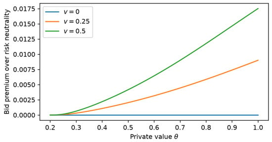
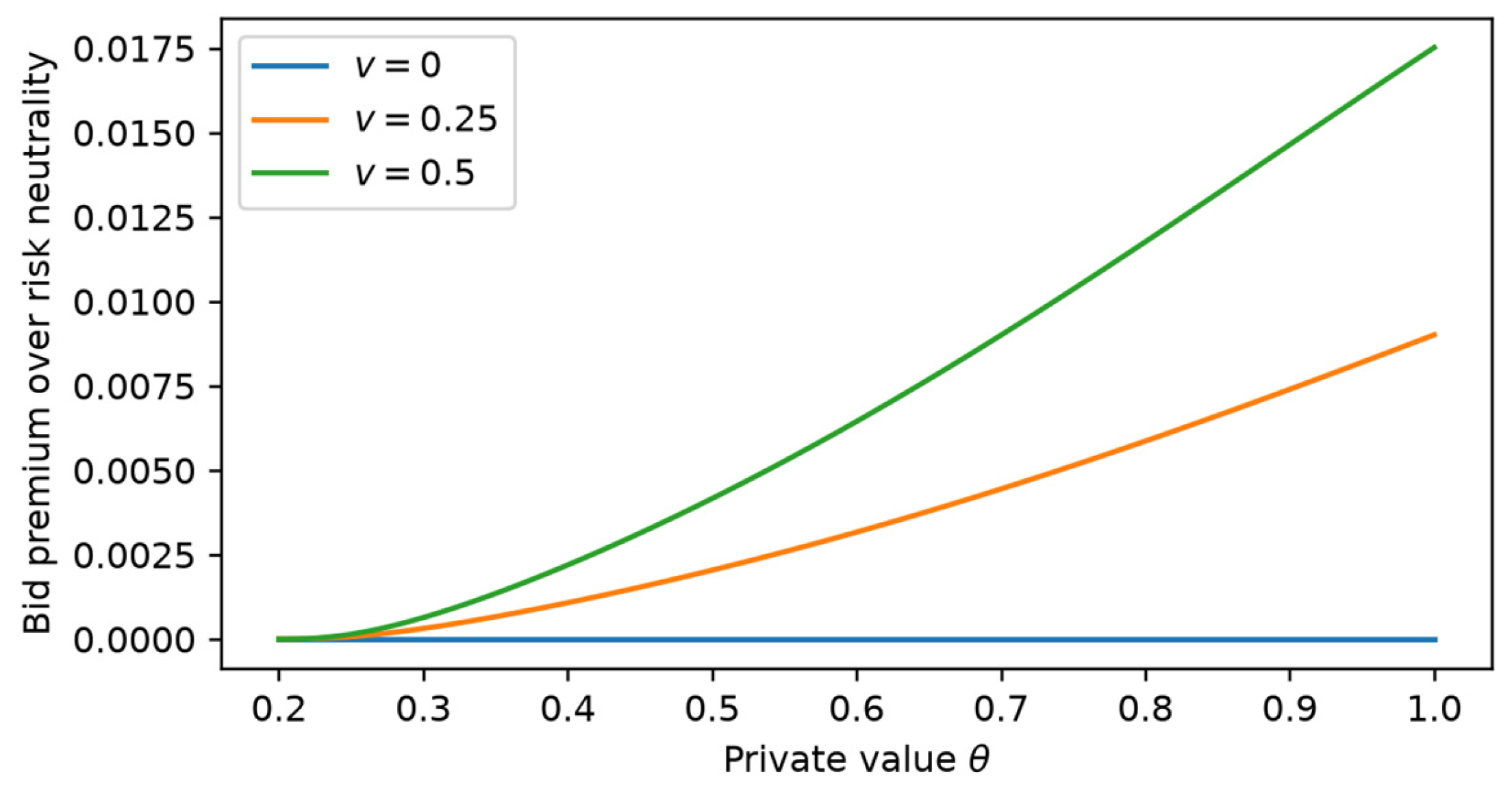
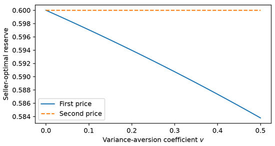
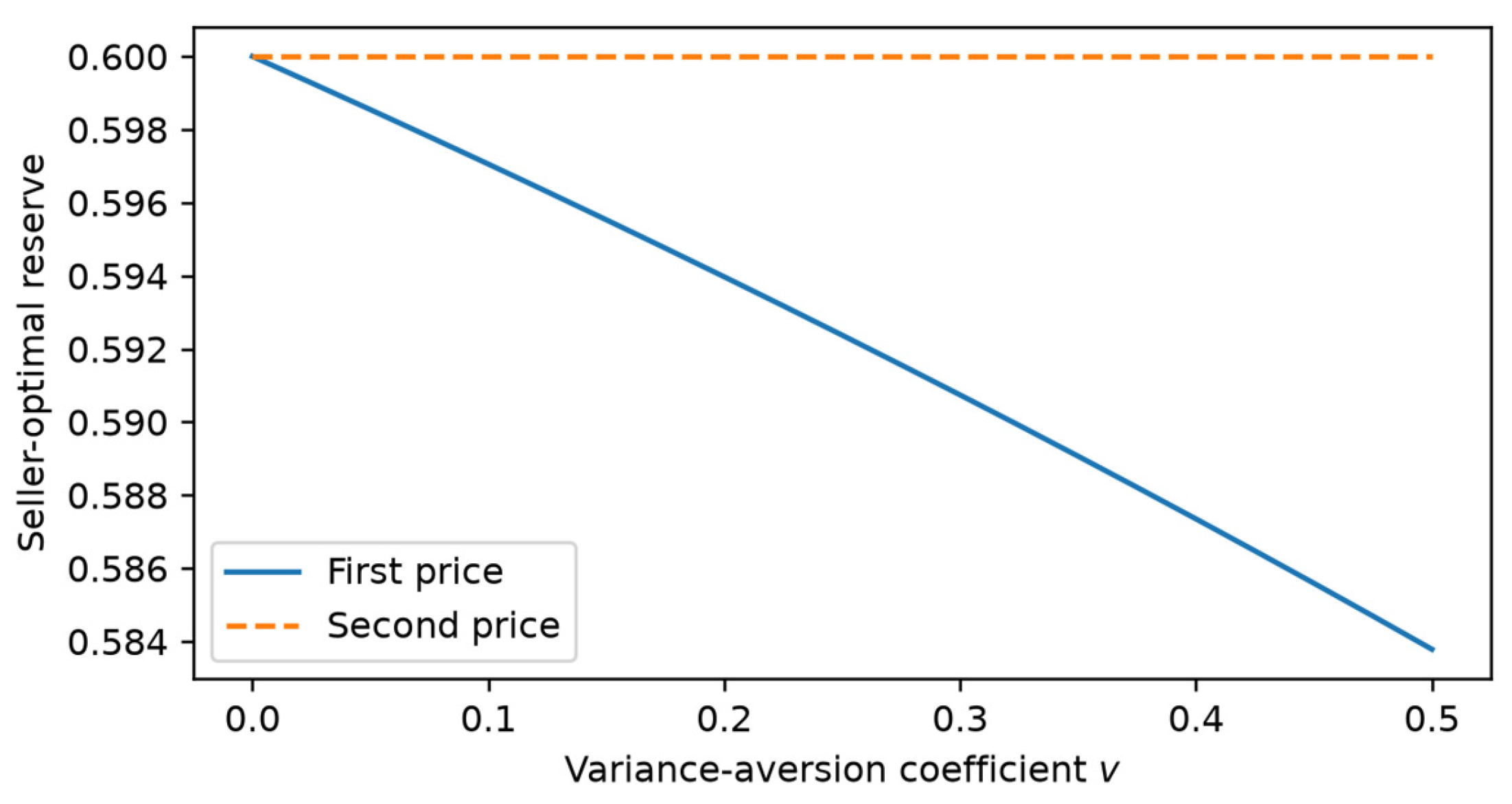
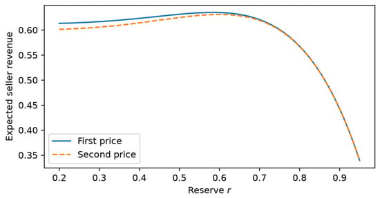
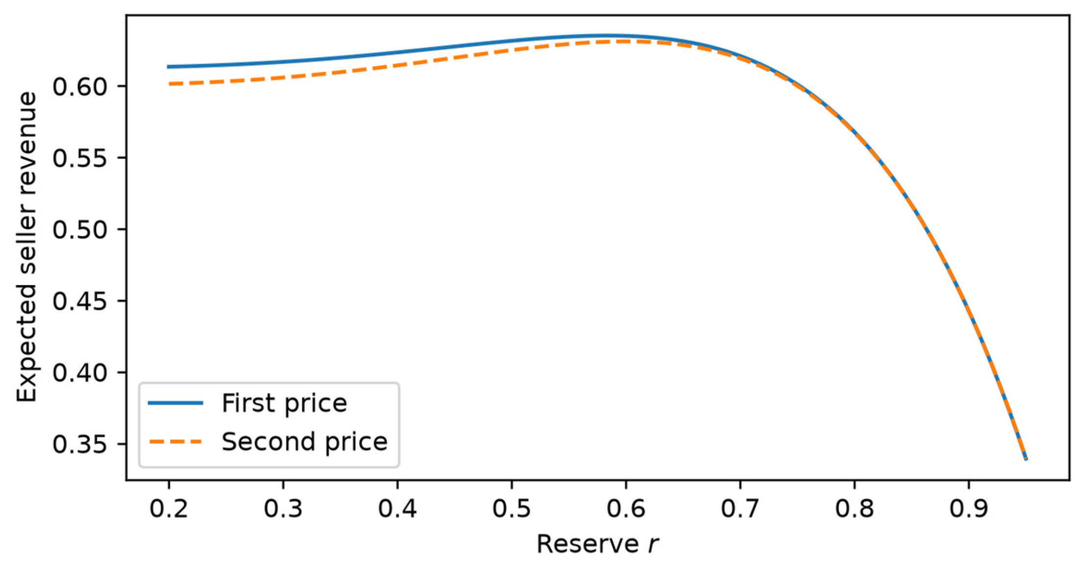
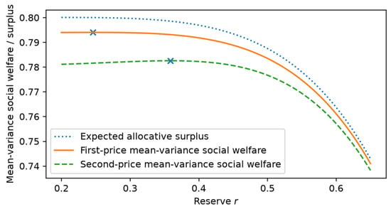
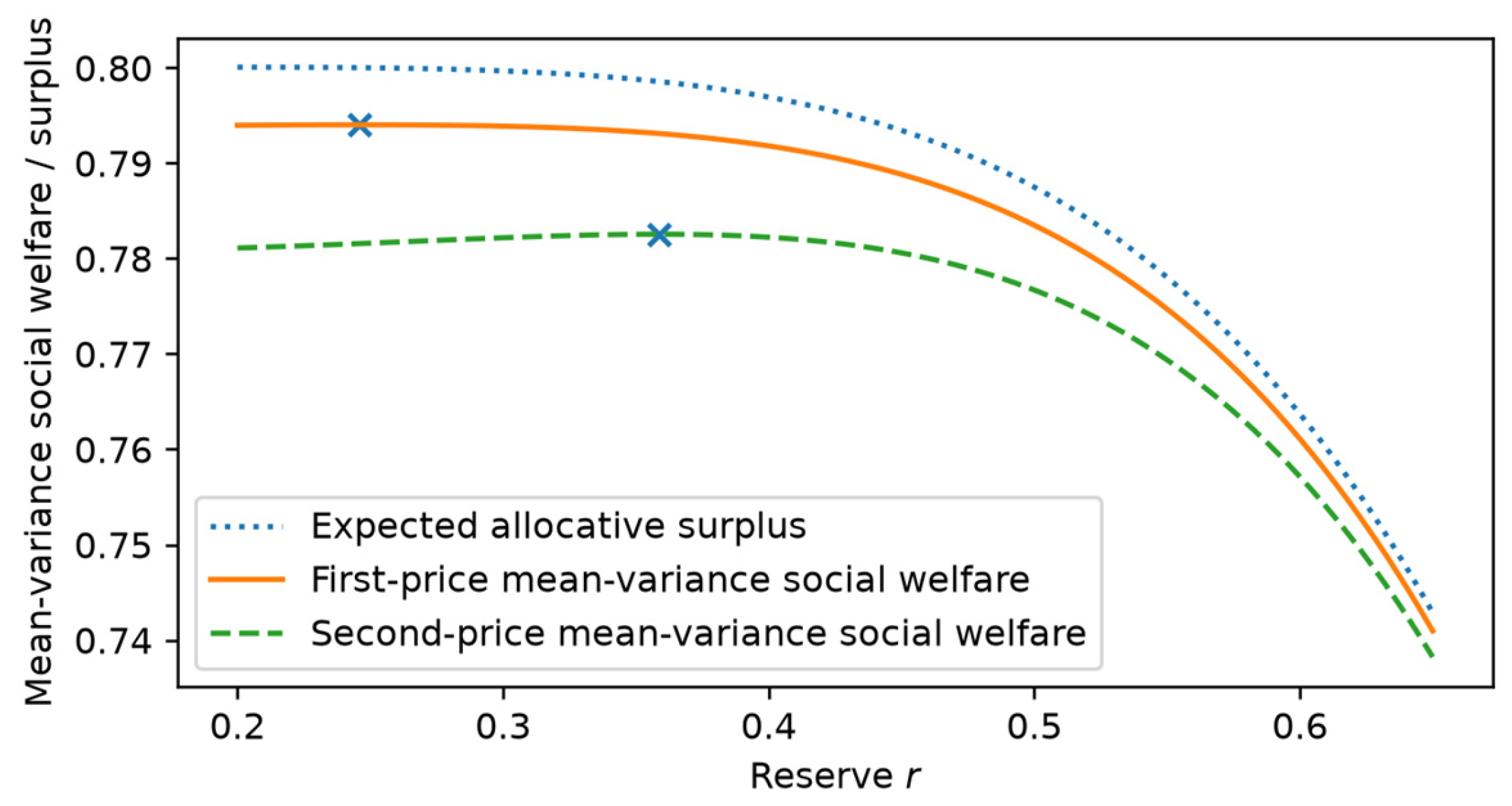
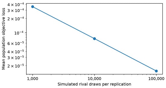
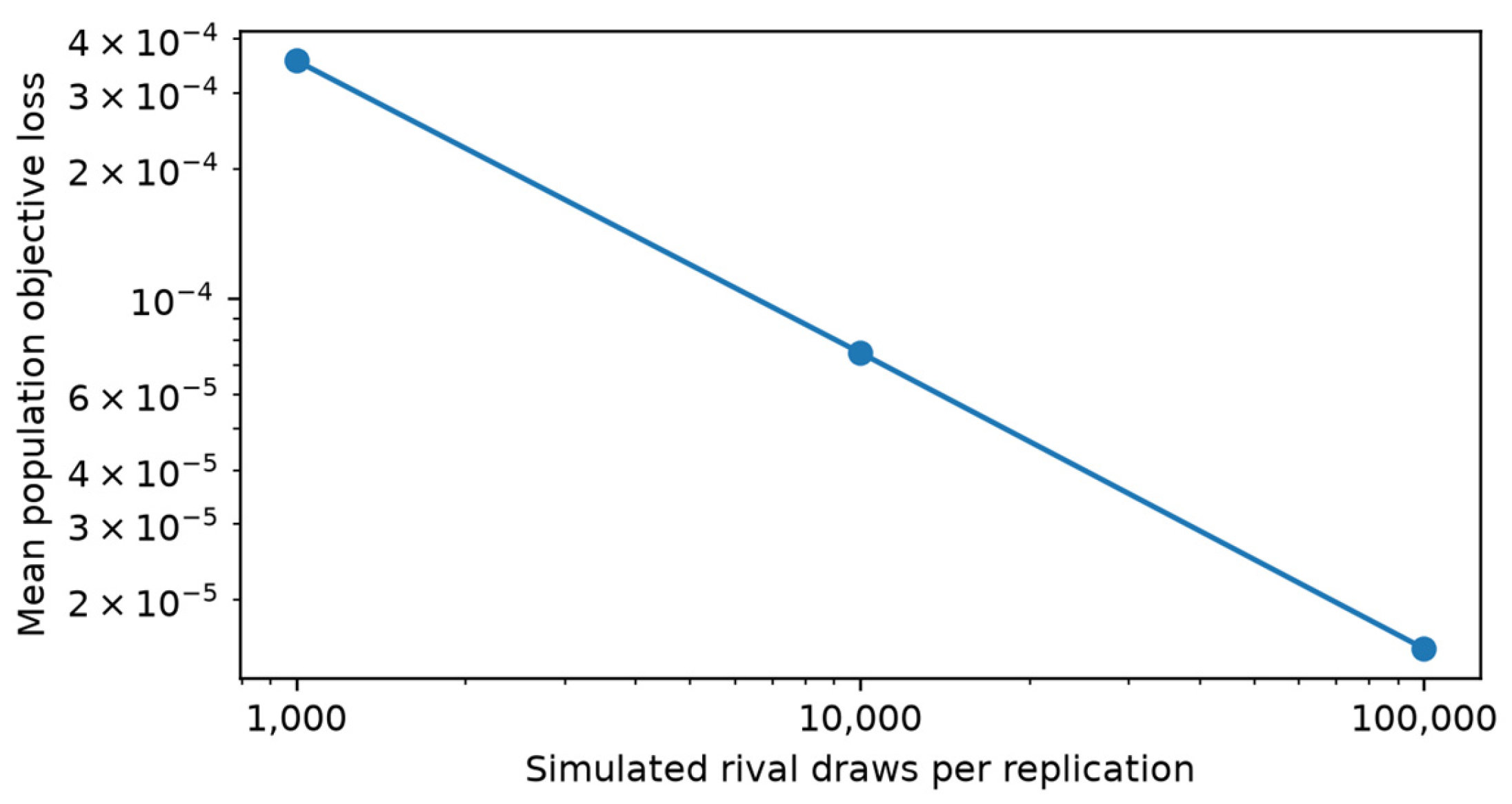

Disclaimer/Publisher’s Note: The statements, opinions and data contained in all publications are solely those of the individual author(s) and contributor(s) and not of MDPI and/or the editor(s). MDPI and/or the editor(s) disclaim responsibility for any injury to people or property resulting from any ideas, methods, instructions or products referred to in the content. |
© 2026 by the authors. Licensee MDPI, Basel, Switzerland. This article is an open access article distributed under the terms and conditions of the Creative Commons Attribution (CC BY) license.