Detrended Multiple Cross-Correlation Analysis of Four Nonstationary Time Series: Formulation and Application to Solar Radiation

Abstract

In this paper, we performed a (multiple) DCCA cross-correlation statistical analysis with the DFA and DCCA methods using the coefficients ${\rho }_{DCCA}$ and ${DMC}_x^2$. Solar radiation was considered the main variable of interest. Understanding multi-scale fluctuations in solar radiation is crucial for climate modeling and predicting weather patterns, and it plays a critical role in environmental processes and human activities. Cross-correlation in the context of solar radiation refers to the statistical relationship or connection between solar radiation and various environmental or atmospheric variables. Analyzing cross-correlations helps to understand how changes in solar radiation relate to other factors over time or across different locations. Thus, we studied an area encompassing almost the entire territory of Brazil, using data from twenty-six automatic weather stations. To achieve this objective, we applied the DCCA multiple cross-correlation coefficient, ${DMC}_x^2$, between solar radiation and (air temperature, relative humidity, and wind speed). To the best of our knowledge, this is the first explicit analytical formulation and application of the ${DMC}_x^2$ coefficient involving one dependent variable and three independent variables. This formulation also enables the construction of multi-scale spatial color maps, revealing persistent multi-scale cross-correlation structures and systematically higher ${DMC}_x^2$ values in northeastern Brazil, not evident from pairwise analyses, or by classical methods.

1. Introduction

Considering that Brazil, with an area of approximately 8.5 million $\mathrm{k}{\mathrm{m}}^2,$ is the fifth largest country in the world, behind Russia, Canada, China, and the United States, the climate is quite diverse, ranging from humid equatorial regions to semi-arid and subtropical areas. The main types of climate found in Brazil are the equatorial climate in the Amazon region, with high humidity and high temperatures throughout the year; the tropical climate in much of the center and east of the country, including the Center-West and Southeast, with a dry winter and rainy summer; the semiarid climate, in the northeastern backlands, with little rain, high temperatures, and long periods of drought; the tropical highland climate in the mountainous regions of the Southeast, such as parts of Minas Gerais and São Paulo, with colder winters and mild summers, and rainfall concentrated in the summer; the subtropical climate, in the southern region, with four well-defined seasons, with hot summers and colder winters. These climate variations directly influence agriculture, biodiversity, and the inhabitants’ way of life, requiring adaptations from natural resource management to urban and agricultural planning to mitigate negative impacts and ensure the resilience of affected communities. In this context, solar radiation is a fundamental component of the Earth’s climate system and plays a central role in several environmental processes, including surface heating, evapotranspiration, atmospheric circulation, and the energy balance of terrestrial ecosystems. Therefore, understanding its multiscale relationships with air temperature, relative humidity, and wind speed is environmentally relevant, since changes in these variables can influence hydrological processes, vegetation dynamics, agricultural activities, and local climatic conditions. The identification of distinct cross-correlation patterns among Brazilian regions also provides useful information for understanding regional atmospheric variability and the interactions between surface and atmospheric processes.

In this paper, we performed a statistical analysis of important meteorological variables from the perspective of their DCCA (multiple) cross-correlations, where global solar radiation is the main component. The choice of this variable can be explained by the fact that solar radiation plays a crucial role in determining the Earth’s climate, influencing everything from global temperature to atmospheric circulation patterns. Cross-correlation analysis provides a quantitative framework for investigating the relationships between solar radiation and atmospheric variables (air temperature, relative humidity, and wind speed) across multiple temporal scales. In this context, multivariate cross-correlation analysis can help characterize how changes in solar radiation relate to other atmospheric factors over time and across different locations. The remainder of the paper is organized as follows. Section 2 presents the classical literature on cross-correlation analysis, Section 3 describes the study area and dataset, Section 4 presents the methodology, Section 5 discusses the results, and Section 6 presents the conclusions.

2. Classical Literature on Cross-Correlations Analysis

A classical reference to time-series analysis and forecasting is Box & Jenkins [1], with a foundational work that established a systematic statistical framework for modeling, analyzing, and forecasting time series data. However, it all begins with one of the oldest works, formalized by Karl Pearson [2]. In this paper, Pearson introduces the product-moment coefficient, with the aim of quantifying the linear relationship between two variables. The coefficient emerges as a generalization of the paper of Francis Galton [3], who already studied regression and association between biological variables. The value of this coefficient ranges from -1 to 1, indicating perfect negative correlation, no correlation, or perfect positive correlation, respectively. However, as time goes by, it becomes clear that there are limitations to this coefficient, such as sensitivity to non-stationarity, spurious correlations, and inability to capture non-linear relationships.

Classic variations of Pearson’s coefficient have been proposed, the most famous being those introduced by Spearman [4] and Kendall [5]. These are non-parametric measures of association, widely used as alternatives to Pearson’s coefficient when the assumptions of linearity, normality, or homoscedasticity are not met. Both assess the monotonic dependence between two variables, being based on the ordering of the data rather than their absolute values.

The Spearman’s coefficient is calculated from Pearson’s correlation applied to the ranks of the observations. This approach makes the measure less sensitive to outliers and suitable for detecting monotonic, linear, or non-linear relationships. The Kendall’s coefficient is based on a pairwise comparison of observations, quantifying the difference between concordant and discordant pairs. Because of this construction, this coefficient has a direct probabilistic interpretation, representing the difference between the probability of agreement and disagreement between two variables.

When more than two variables are involved, we can apply the multivariate cross-correlation analysis. In the classical approach, multi-cross correlation deals with the linear dependence between multiple time series or multiple random variables. It naturally arises as an extension of bivariate cross-correlation to the multivariate case, which is well developed in [6,7,8]. In this sense, we have excellent textbooks, such as:

• Priestley [9], which offers a fundamental framework for the study of multivariate time series by representing stochastic processes in the frequency domain. In this context, cross-spectral densities and coherence functions are key tools for quantifying linear dependence, phase relationships, and coupling among multiple series. Spectral methods allow the identification of dominant frequencies and shared oscillatory components that are not evident in the time domain. These concepts provide the theoretical foundation for multivariate prediction and control, enabling the design of filters and controllers that minimize mean-square error in complex stochastic systems;
• Brillinger [10], which employs basic techniques of univariate and multivariate statistics for the analysis of time series and signals. It provides a broad collection of theorems, placing the techniques on firm theoretical ground. The techniques, which are illustrated by data analyses, are discussed in both a heuristic and a formal manner, making the book useful for both the applied and the theoretical worker. It considers second- and higher-order parameters and estimates them equally, thereby handling non-Gaussian series and nonlinear systems directly.

However, when it comes to having more robust time series analysis for bivariate cross-correlations, we can employ more recent methods. Among these methods, we highlight here the DCCA, proposed by Podobnik & Stanley [11], which removes local trends and evaluates cross-correlation at different time scales (as we can see briefly in Section 4.1). The generalization of the DFA method proposed by Zebende, for cross-correlation analysis between multiple time series, is interesting and can be determined by the DCCA cross-correlation coefficient [12] in its generic form [13]. In this case, the Detrended Multiple Cross-Correlation Coefficient is a scale-dependent measure designed to quantify the strength of collective cross-correlations among multiple non-stationary time series. It extends the detrended cross-correlation analysis (DCCA) from the bivariate case to a multivariate framework by incorporating several variables simultaneously. This multivariate approach is particularly relevant for climate-related applications, where several atmospheric variables may exhibit scale-dependent relationships.

3. Area of Study and Data

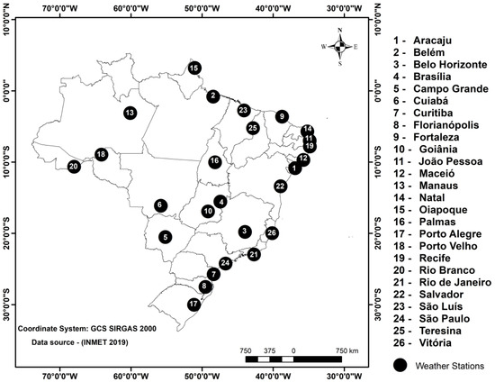
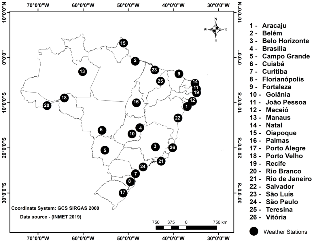
Our area of study covers practically the entire territory of Brazil, as can be seen in Figure 1.

Figure 1. Map of Brazil with twenty-six automatic weather stations operated by INMET [14].

Each point in this figure corresponds to the geographic location of one of the twenty-six weather stations, where the environmental variables were measured hourly. Some stations are located at altitudes close to sea level: 1- Aracaju (3.72 $\mathrm{m})$, 8- Florianópolis (4.87 $\mathrm{m}$), and 26- Vitória (9 $\mathrm{m}$). Other stations are located at high altitudes, such as 4- Brasília (1160.96 $\mathrm{m}$), 7- Curitiba (922.91 $\mathrm{m}$), and 3- Belo Horizonte (854.02 $\mathrm{m}$). The data were obtained and validated by INMET, the Brazilian Institute of Meteorology [14]. INMET aims to obtain as much meteorological information as possible from the entire Brazilian territory through monitoring, analysis, and weather and climate forecasting, with an emphasis on practical and reliable results. The data collected by INMET are freely available and can be downloaded directly from: https://portal.inmet.gov.br/.

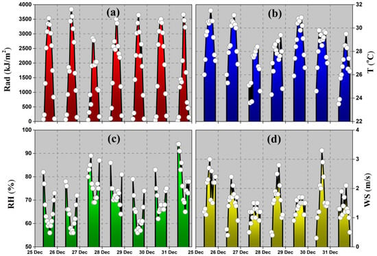
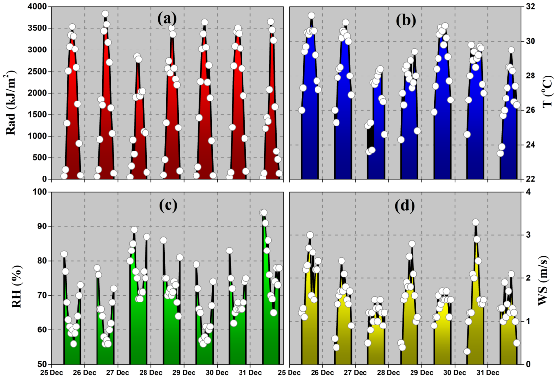
We downloaded four meteorological variables (hourly) from the INMET public site: solar radiation, air temperature, relative humidity, and wind speed. For the reasons described above, we emphasize solar radiation, which, for the present analysis, was considered between 09:00 and 21:00 UTC, the time of day when there is still solar radiation penetrating the meteorological sensor (pyranometer); see [15]. Our analysis period was between 1 January 2009, and 12 December 2019. As one example, Figure 2 show for illustrative purposes and is outside the analysis period, a week’s worth of data for Salvador station.

Figure 2. (Color online) Four weather variables: (a) solar radiation, Rad ($\mathrm{k}\mathrm{J}/$${\mathrm{m}}^2$), (b) Air temperature T ($°\mathrm{C}$), (c) relative humidity RH (%), and (d) wind speed WS ($\mathrm{m}{\mathrm{s}}^{-1}$), as a function of time (hours). This example was taken from Salvador station between 25 December 2019 and 1 January 2020. The black line represents the average value over the stations and is included to facilitate comparison.

The results show a positive (negative) relationship between solar radiation and air temperature (relative humidity), but between these same variables and wind speed, there is no clarity to decide whether or not there is a relationship (cross-correlation) between them. Thus, a more accurate statistical analysis may be valuable at this point, which was performed after introducing the study methodology shown below.

4. Methodology

The statistical methodology used to analyze the DCCA multiple cross-correlations is briefly described below in Section 4.1, Section 4.2 and Section 4.3. Here, in these methods, we apply the overlapping boxes to improve the sampling of the fluctuation functions and the resolution of the scale-dependent estimates rather than to artificially increase the effective sample size.

4.1. Detrended Fluctuation Analysis

The Detrended Fluctuation Analysis (DFA) method is based on the algorithm described below in 6 basic steps [16]:

(i)

Consider (for example) the time series of solar radiation, $\left\{x_i\right\}$ (in $\mathrm{k}\mathrm{J}/$${\mathrm{m}}^2$), with $i=1,...,N_{max}$ (time series length). We integrate $x_i$ to obtain $X_k={\sum }_{i=1}^k[x_i-<x>]$, where $<x>$ is the mean of x and $k=1,...,N_{max}$;

(ii)

The signal, $X_k$, is divided into $(N_{max}-n)$ overlapping boxes of equal length n (time-scale). Each box contains $(n+1)$ values that start at i and end at $(i+n)$;

(iii)

For each box, we compute the local trend (a linear least-squares fit) of $X_k$ in order to obtain the adjusted value, ${\tilde{X}}_{k,i}$, with $(i\le k\le i+n)$;

(iv)

The integrated signal, $X_k$, is subtracted by ${\tilde{X}}_{k,i}$ (detrended) to obtain:

$$f_{DFA}^2(n,i)=1/(n+1){\displaystyle \sum _{k=i}^{i+n}}{(X_k-{\tilde{X}}_{k,i})}^2;$$

(1)

(v)

For a given time-scale of length n, $F_{DFA}\left(n\right)$ is calculated as follows:

$$F_{DFA}\left(n\right)=\sqrt{{\displaystyle \frac{1}{(N_{max}-n)}}{\displaystyle \sum _{i=1}^{N_{max}-n}}{f}_{DFA}^2(n,i)};$$

(2)

(vi)

The above steps are repeated for a broad range of time-scales, (the smallest) $4\le n\le N_{max}/4$ (the largest), to provide a relationship between $F_{DFA}$ and n.

For more details about the DFA algorithm, see: https://physionet.org/content/dfa/1.0.0/, accessed on 19 September 2026.

If a long-range auto-correlation appears, then $F_{DFA}\sim n^{{\alpha }_{DFA}}$, where ${\alpha }_{DFA}$ is a self-affinity parameter that represents the long-range auto-correlation, see [17]. The DFA method is able to identify the seasonal components of a signal, and $F_{DFA}\left(n\right)$ can be applied to distinguish different types of signals.

However, if we want to analyze cross-correlation, we can apply the DFA generalization that will be presented below, in conjunction with its coefficient ${\rho }_{DCCA}$.

4.2. DCCA Cross-Correlation Coefficient

Using two-time series $\left\{x_i\right\}$ and $\left\{y_i\right\}$ of equal length $N_{max}$, we defined and calculated the following equations for these time series:

$$X_k={\sum }_{i=1}^k[x_i-<x>] \mathrm{a}\mathrm{n}\mathrm{d} Y_k={\sum }_{i=1}^k[y_i-<y>],$$

where $k=1,\cdots ,N_{max}$. Then, we generalized the DFA algorithm (the six steps described above) to find the covariance of the residuals (inside each box), or better yet:

$$f_{DCCA}^2(n,i)\equiv 1/(n+1){\sum }_{k=i}^{i+n}(X_k-{\tilde{X}}_{k,i})(Y_k-{\tilde{Y}}_{k,i})$$

and the detrended covariance function (for all boxes):

$$F_{DCC{A}_{xy}}^2\left(n\right)\equiv {(N_{max}-n)}^{-1}{\displaystyle \sum _{i=1}^{N_{max}-n}}{f}_{DCCA}^2(n,i).$$

(3)

This is the fluctuation function, which tells us whether or not there is cross-correlation between these two time series and the type of behavior, see [11]. However, to quantify the level of cross-correlation, the DCCA cross-correlation coefficient can be defined as the ratio between the detrended cross-correlation function $F_{DCCA}^2$ and the detrended auto-correlation function $F_{DFA}$ for $\left\{x_i\right\}$ and $\left\{y_i\right\}$, see [12]:

$${\rho }_{DCCA}\left(n\right)\equiv {\displaystyle \frac{F_{DCC{A}_{xy}}^2\left(n\right)}{F_{DF{A}_x}\left(n\right)F_{DF{A}_y}\left(n\right)}}$$

(4)

Some important properties of ${\rho }_{DCCA}$ occur naturally, the most basic of which is:

$$-1.0\le {\rho }_{DCCA}\le 1.0$$

Consequently, ${\rho }_{DCCA}=0.0$ means that there is no cross-correlation between $\left\{x_i\right\}$ and $\left\{y_i\right\}$, and it divides the level of cross-correlation between the positive and negative cases. This coefficient has been tested on selected time series [18] and is quite robust, especially for statistical analyses of non-stationary time series [19,20,21,22]. Therefore, using the instantaneous air temperature measured at 12 meteorological stations, we can apply the methodology described above and analyze the results.

4.3. DCCA Multiple Cross-Correlation Coefficient

The DCCA multiple cross-correlation coefficient, ${DMC}_x^2$, is a generalization of the traditional DCCA method to analyze multiple non-stationary time series [13]. This approach enables us to examine the interdependence between multiple time series simultaneously, rather than just two. This is especially useful in studies of complex systems where many variables may be correlated in a non-trivial way because this coefficient allows for the identification of the presence and intensity of multiple cross-correlations between these time series.

A brief description of ${DMC}_x^2$ with some applications follows. The Detrended Multiple Cross-Correlation Coefficient quantifies the multiple cross-correlation between one time series $\left\{Y\right\}$, defined as the target variable, and k other time series $\left\{X_1\right\}$, $\left\{X_2\right\}$, $\left\{X_3\right\}$, …, $\left\{X_k\right\}$, defined as explanatory variables. Its mathematical expression is defined as:

$${DMC}_x^2\left(n\right)\equiv {\rho }_{Y,X_i}{\left(n\right)}^T\times {\rho }^{-1}\left(n\right)\times {\rho }_{Y,X_i}\left(n\right)$$

(5)

In this equation, ${\rho }^{-1}\left(n\right)$ represents the inverse matrix of all possible combinations of ${\rho }_{DCCA}$ between the independent variables:

$${\rho }^{-1}\left(n\right)={\left(\begin{array}{ccccc}1& {\rho }_{X_1,X_2}\left(n\right)& {\rho }_{X_1,X_3}\left(n\right)& \dots & {\rho }_{X_1,X_k}\left(n\right)\\ {\rho }_{X_2,X_1}\left(n\right)& 1& {\rho }_{X_2,X_3}\left(n\right)& \dots & {\rho }_{X_2,X_k}\left(n\right)\\ ⋮& ⋮& ⋮& \dots & ⋮\\ {\rho }_{X_k,X_1}\left(n\right)& {\rho }_{X_k,X_2}\left(n\right)& {\rho }_{X_k,X_3}\left(n\right)& \dots & 1\end{array}\right)}^{-1}$$

(6)

The main diagonal in Equation (6) is 1 (one) because ${\rho }_{X_a,X_a}$ between the time series $\left\{X_a\right\}$ with itself has the maximum value. By definition, ${\rho }_{X_a,X_b}={\rho }_{X_b,X_a}$, and this makes the matrix symmetric with respect to its main diagonal. Also,

$${\rho }_{Y,X_k}{\left(n\right)}^T=[{\rho }_{Y,X_1}\left(n\right),{\rho }_{Y,X_2}\left(n\right),\cdots ,{\rho }_{Y,X_k}\left(n\right)]$$

(7)

represents the transposed vector of the ${\rho }_{Y,X_i}\left(n\right)$ between the target (dependent) variable $\left\{Y\right\}$ and each independent variable $\left\{X_i\right\}$. The DCCA multiple cross-correlation coefficient has been applied in many problems, specifically for three variables, i.e, one target (dependent) variable $\left\{Y\right\}$ and two independent variables $\left\{X_1\right\}$, $\left\{X_2\right\}$. Examples of these applications can be found applied to meteorological variables [15], in statistical tests [23,24], among other applications.

To the best of our knowledge, we found no previous study explicitly deriving and applying the particular case of four time series, with one target (dependent) variable $\left\{Y\right\}$ and three independent variables $\left\{X_1\right\}$, $\left\{X_2\right\}$, $\left\{X_3\right\}$, which is what we propose here.

Starting from Equation (5), we derive the explicit analytical expression of the ${DMC}_x^2$ coefficient for one target (dependent) variable and three independent variables, given by Equation (9), with $\Delta$ defined by:

$$\Delta \equiv 1+2{\rho }_{X_1,X_2}{\rho }_{X_1,X_3}{\rho }_{X_2,X_3}-{\rho }_{X_1,X_2}^2-{\rho }_{X_1,X_3}^2-{\rho }_{X_2,X_3}^2.$$

(8)

$$\begin{array}{cc}\hfill DM{C}_x^2={\displaystyle \frac{1}{\Delta }}[& \left(1-{\rho }_{X_2,X_3}^2\right){\rho }_{Y,X_1}^2+\left(1-{\rho }_{X_1,X_3}^2\right){\rho }_{Y,X_2}^2+\left(1-{\rho }_{X_1,X_2}^2\right){\rho }_{Y,X_3}^2\hfill \\ \hfill & +2\left({\rho }_{X_1,X_3}{\rho }_{X_2,X_3}-{\rho }_{X_1,X_2}\right){\rho }_{Y,X_1}{\rho }_{Y,X_2}\hfill \\ \hfill & +2\left({\rho }_{X_1,X_2}{\rho }_{X_2,X_3}-{\rho }_{X_1,X_3}\right){\rho }_{Y,X_1}{\rho }_{Y,X_3}\hfill \\ \hfill & +2\left({\rho }_{X_1,X_2}{\rho }_{X_1,X_3}-{\rho }_{X_2,X_3}\right){\rho }_{Y,X_2}{\rho }_{Y,X_3}].\hfill \end{array}$$

(9)

Equation (9) represents the first explicit analytical expression of the ${DMC}_x^2$ coefficient for four non-stationary time series.

The data mining, the calculations, and the results are presented in the next section. Here, the idea is to use the above methodology to analyze, in (multiple) pairs, the cross-correlations between the meteorological variables: solar radiation, air temperature, relative humidity, and wind speed, because they are the main elements of the climate and are easily accessible.

5. Results and Discussions

Our analysis period was between 1 January 2009, and 12 December 2019, representing approximately 10 years of hourly measurements. We begin the analysis with the descriptive statistics, focusing on describing and summarizing the main characteristics of our data set.

5.1. Descriptive Statistics

Table 1 presents our complete data sample from all weather stations, showing the minimum and the maximum values of solar radiation (Rad), air temperature (T), relative humidity (RH), and wind speed (WS).

Table 1. Maximum and minimum solar radiation (Rad), air temperature (T), relative humidity (RH), and wind speed (WS) values for all stations.

	Rad (kJ/m2)		T (°C)		RH (%)		WS (m s−1)
	Min	Max	Min	Max	Min	Max	Min	Max
Aracaju	0.0	3960.7	19.6	35.4	10	100	0.0	8.7
Belém	0.0	5230.0	21.4	37.0	32	100	0.0	7.2
Belo Horizonte	0.0	5246.5	7.7	37.0	10	97	0.0	10.2
Brasília	0.0	4414.8	9.6	34.8	10	100	0.0	10.4
Campo Grande	0.0	4988.4	4.3	39.8	11	100	0.0	12.1
Cuiabá	0.0	4113.5	9.1	41.4	10	99	0.0	8.4
Curitiba	0.0	4101.5	0.1	34.1	13	100	0.0	9.4
Florianópolis	0.0	4184.4	5.1	39.3	18	97	0.0	10.6
Fortaleza	0.0	3810.6	20.1	34.4	29	100	0.0	14.6
Goiânia	0.0	4341.4	6.0	39.1	9	97	0.0	9.7
João Pessoa	0.0	4884.3	19.6	32.7	36	96	0.1	7.3
Maceió	0.0	4694.6	17.2	36.3	33	96	0.1	8.5
Manaus	0.0	3867.9	20.6	40.4	23	100	0.1	7.9
Natal	0.1	4765.2	20.3	32.3	41	98	0.0	10.5
Oiapoque	0.0	3993.5	19.5	36.7	29	100	0.1	5.6
Palmas	0.0	3969.7	17.2	41.6	10	100	0.0	12.2
Porto Alegre	0.0	3999.9	0.8	40.2	18	100	0.0	8.9
Porto Velho	0.0	4153.2	15.5	37.8	19	98	0.1	19.9
Recife	0.0	4898.8	18.0	34.4	28	100	0.0	5.2
Rio Branco	0.0	6682.6	9.2	38.2	10	100	0.0	10.9
Rio de Janeiro	0.0	5308.3	14.5	38.8	13	100	0.0	17.2
Salvador	0.0	4446.0	19.2	35.3	42	97	0.0	6.6
São Luís	0.0	7850.2	21.2	34.1	32	100	0.0	5.8
São Paulo	0.0	3999.9	4.5	37.0	10	100	0.0	10.9
Teresina	0.0	3901.7	17.1	40.8	13	99	0.0	8.7
Vitória	0.0	4193.5	12.6	37.5	25	100	0.1	6.7
Global Mean	0.0	4267.5	16.3	37.0	18.0	100.0	0.0	9.2

Table 1 shows that solar radiation has a minimum value (zero) for all stations; its maximum value was 7850.2 $\mathrm{k}\mathrm{J}/$${\mathrm{m}}^2$ at the São Luís station. The minimum air temperature was recorded at the Curitiba station (0.1 $°\mathrm{C}$) and the maximum was recorded at the Palmas station (41.6 $°\mathrm{C}$). Regarding the relative humidity, it can be said that the minimum value was recorded at the Goiânia station (9%) and the maximum was recorded at most stations. Lastly, in relation to the wind speed, most stations recorded a minimum value of zero; the highest value was recorded at the Rio de Janeiro station (17.2 $\mathrm{m}{\mathrm{s}}^{-1}$). We can see considerable variation (large amplitudes) in these results. The last row of Table 1 shows the mean value for each column, giving a global meteorological view of the Brazilian territory.

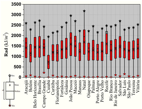
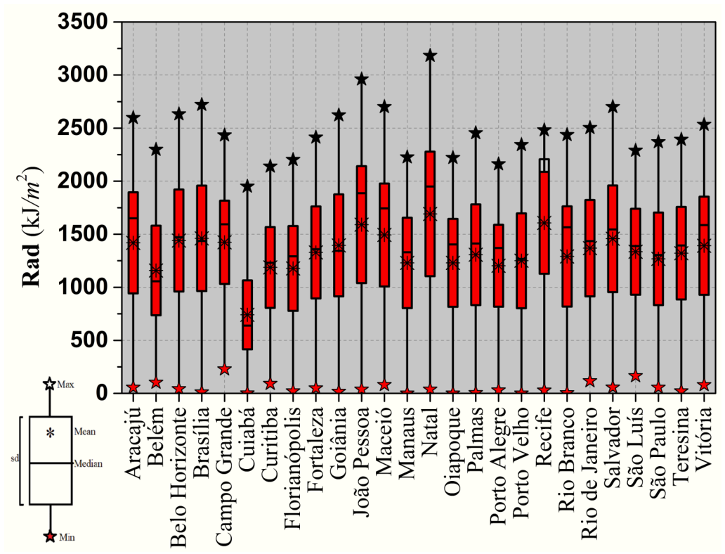
From the point of view of the entire temporal sample, we take the mean values for all variables, from 9 to 21 h UTC. After obtaining these mean values, we made a box plot for each station (in the UTC time interval). These box plots show the mean, median, standard deviation, and minimum and maximum values (see inset in Figure 3).

Figure 3. (Color online) Box plot for the solar radiation (mean values) for all 26 stations from 9 to 21 UTC hour.

Figure 3 presents the mean values for solar radiation.

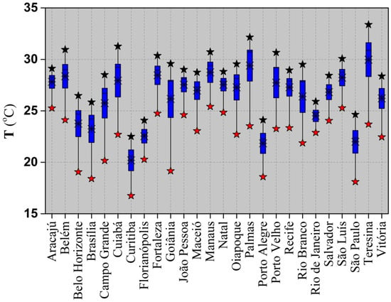
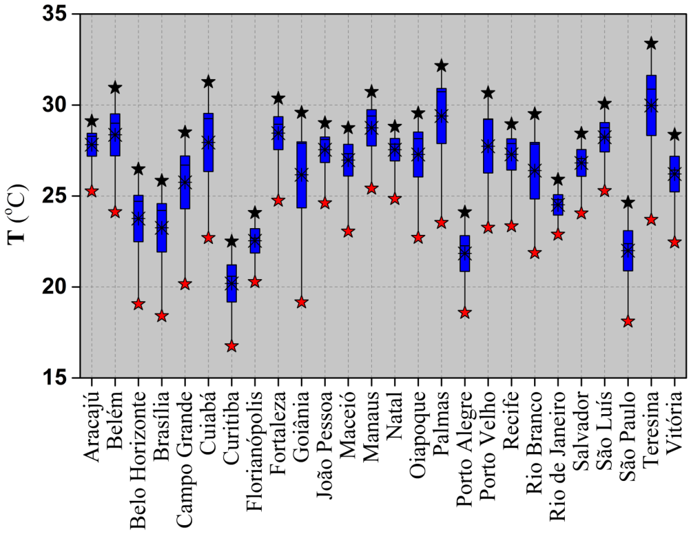
It shows that the mean value of solar radiation has a high amplitude, in the order of 2500 $\mathrm{k}\mathrm{J}/$${\mathrm{m}}^2,$ with Cuiabá (minimum) and Natal station (maximum) as its extremes. Similarly, Figure 4 presents the mean values for air temperature.

Figure 4. (Color online) Box plot for the air temperature (mean values) for all 26 stations from 9 to 21 h UTC.

We can observe the variation in air temperature as a function of geographic location. For instance, Curitiba exhibits the lowest values, while Teresina station shows the highest values for both the global mean and the minimum and maximum temperatures.

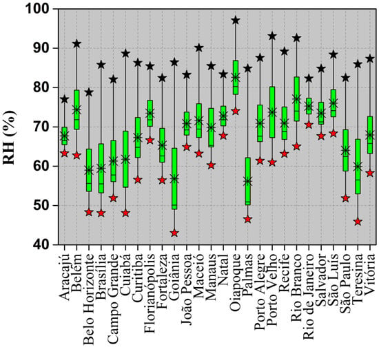
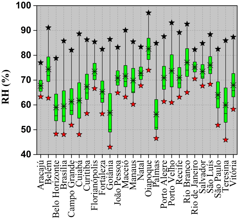
The relationship between solar radiation and relative humidity is indirect, but significant. Solar radiation affects temperature and evaporation, which in turn influence relative humidity, generally leading to an inverse relationship. We also investigate the global mean of relative humidity by station; the results are presented in Figure 5.

Figure 5. (Color online) Box plot for the relative humidity (mean values) for all 26 stations from 9 to 21 h UTC.

It is known that when relative humidity remains below 60%, some conditions can affect health, comfort, and the environment. Below this level, the air is considered dry, which has direct consequences, such as an increase in the sensation of heat, increased fire risk, and rapid loss of soil moisture. The stations located in Belo Horizonte, Brasília, Goiania, Palmas, and Teresina have a global mean of relative humidity below 60%, with the vast majority having values between 60% and 80%. Oiapoque station, in the northernmost part of the state of Amapá, has a global mean for this variable above 80%.

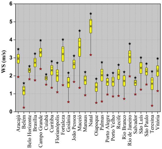
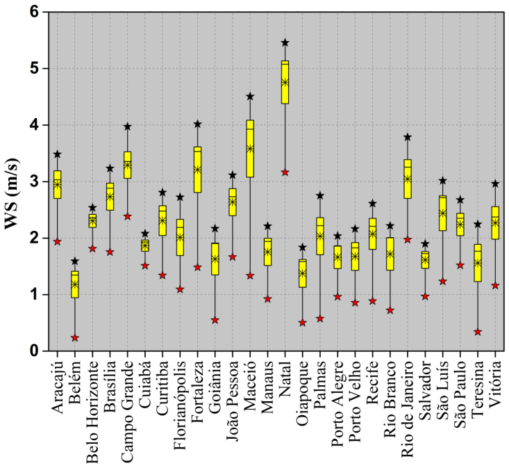
And, as an outcome of this statistical analysis, Figure 6 shows the box plot for the wind speed.

Figure 6. (Color online) Box plot of the wind speed (mean values) for all 26 stations from 9 to 21 h UTC.

The wind speed acts as a temperature moderator because it dissipates heat accumulated at the surface and in the air layer close to the Earth, helping to cool the environment. In areas with high solar radiation, wind speed can alleviate the sensation of heat by increasing the exchange of warm air with cooler air at higher altitudes. Figure 6 demonstrates that among the stations considered, Belém exhibited the lowest mean wind speed, whereas Natal exhibited the highest.

It can be stated that solar radiation, air temperature, relative humidity, and wind speed are not independent variables, and they shape the local climate and thermal sensation. Solar radiation heats the surface, increasing the air temperature, while the wind moderates this effect, dispersing heat and influencing comfort levels. The interaction of these elements can vary widely depending on the location, time of year, and atmospheric conditions. In this sense, it is interesting to assess the relationship between them, especially if we take solar radiation as our target variable. For this objective, we applied the DCCA (multiple) coefficient, with the results presented in the Figure 7 and Figure 8.

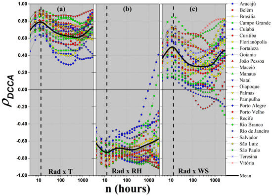
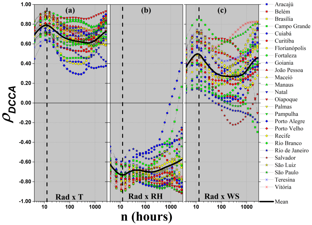
Figure 7. (Color online) ${\rho }_{DCCA}$ as a function of the time-scale n for all stations. The DCCA cross-correlation between (a) Rad × T, (b) Rad × RH, and (c) Rad × WS can be seen. The vertical dashed line corresponds to the 13-h time-scale considered in the analysis.

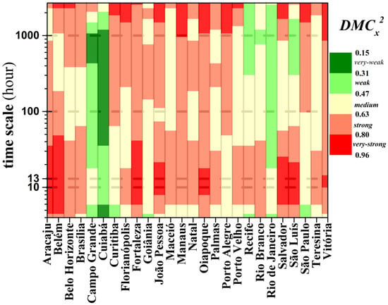
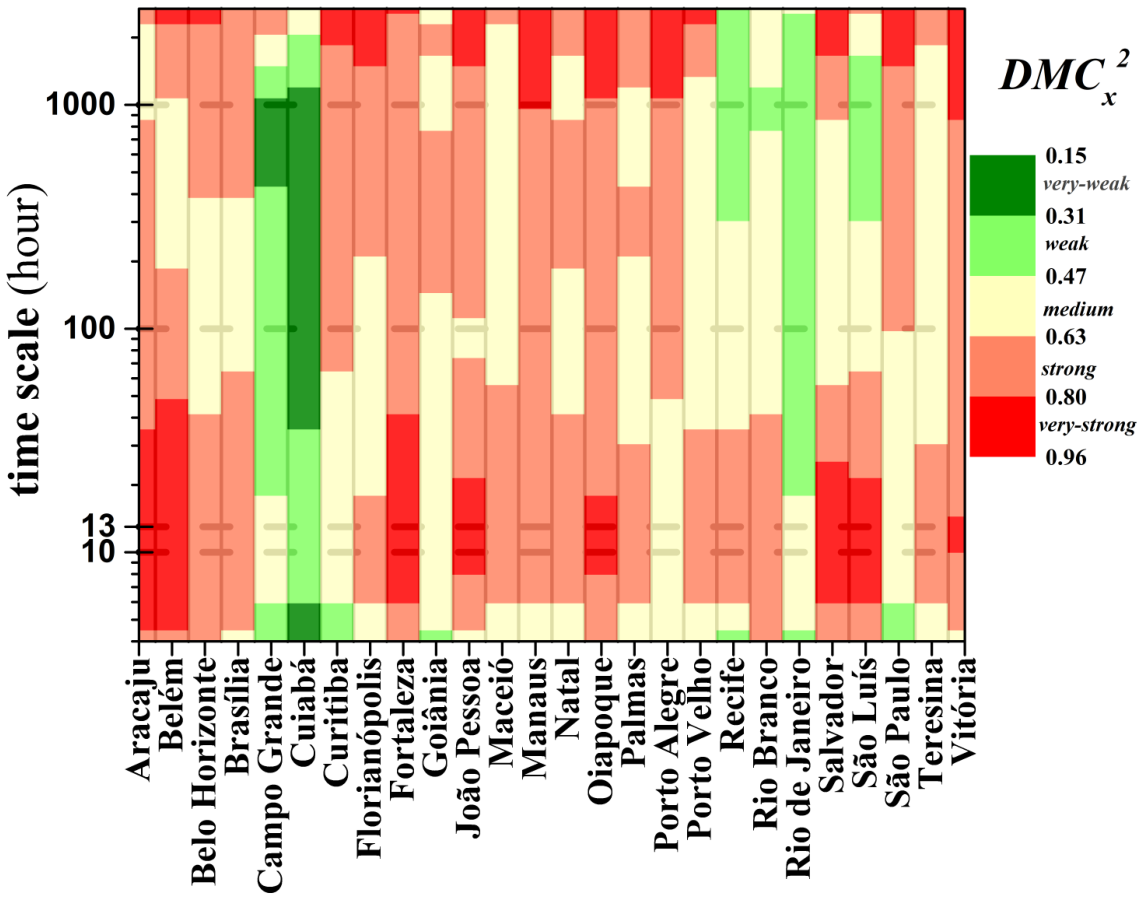
Figure 8. (Color online) Color gradient map (vertical direction) with ${DMC}_x^2$ for all stations. ${DMC}_x^2$ ranges from 0 (green) to 1 (red), with five color levels (see labels).

5.2. DCCA Cross-Correlation Results

The relationship between two time series (mutual relations), by ${\rho }_{DCCA}$, is shown in Figure 7. This figure presents the results for ${\rho }_{DCCA}$ as a function of n for DCCA cross-correlation between: (a) solar radiation (Rad) × air temperature (T), (b) solar radiation (Rad) × relative humidity (RH), and (c) solar radiation (Rad) × wind speed (WS).

The figure shows that the cross-correlation between solar radiation and air temperature is always positive with $0.0<{\rho }_{DCCA}<1.0$, and the DCCA cross-correlation varies depending on the geographic location of each station and the time-scale analyzed. Now, if we look at the cross-correlation between solar radiation and relative humidity, we identify the opposite behavior to the previous one, that is, the coefficient remains negative across the temporal scales and stations analyzed, $-1.0<{\rho }_{DCCA}<0.0$, also, see that this negative value varies according to the location and the time-scale analyzed. However, the cross-correlation between solar radiation and wind speed generally presents a positive value for ${\rho }_{DCCA}$, but with a high amplitude of variation compared to Rad × T. Also, the mean value of ${\rho }_{DCCA}$ was calculated and appears in Figure 7 as the solid black line. The mean of the DCCA cross-correlation coefficient reaches its maximum (minimum) at $n=13$, corresponding to the 13-h temporal scale considered in the analysis.

However, if we want to measure the multiple cross-correlations between all time series, we can apply the multiple coefficient, which we will see next with the ${DMC}_x^2$ value.

5.3. DCCA Multiple Cross-Correlation Results

Figure 8 presents the results for DCCA multiple cross-correlation, with solar radiation as a target (dependent) variable.

In this five-level color map, if:

• ${DMC}_x^2=0$: there is no DCCA multiple cross-correlation between solar radiation × (air temperature; relative humidity; wind speed);
• ${DMC}_x^2=1$: there is a total DCCA multiple cross-correlation between solar radiation × (air temperature; relative humidity; wind speed).

Therefore, from this point of view and based on the time-scale of $n=13$ h (found in Figure 7), we classified the stations according to ${DMC}_x^2$, see the color map in Figure 8. Here, we were able to classify the cross-correlations between air temperature, relative humidity, wind speed, and solar radiation. As a starting point, this classification uncovered an interesting multiple cross-correlation pattern: the stations located in the Brazilian northeast generally had higher ${DMC}_x^2$ values than stations in the Central West, Southeast, and South.

6. Conclusions

In this paper, we performed a multiple DCCA cross-correlation analysis of meteorological variables obtained from twenty-six automatic stations spread across the entire Brazilian territory. This task was done using the coefficient ${DMC}_x^2$, with short- and long-term (multiple time-scales) being studied. We began by analyzing descriptive statistics, which provided the mean, minimum, and maximum values for all meteorological stations and variables, including solar radiation, air temperature, relative humidity, and wind speed. Then, using the DCCA cross-correlation (between pairs), we measured how solar radiation relates to other environmental variables. We found that the value of ${\rho }_{DCCA}$ is positive (negative) between solar radiation and air temperature (relative humidity), and that, in general, ${\rho }_{DCCA}$ depends on the geographical location of stations and the time-scale involved. The value of ${\rho }_{DCCA}$ for the cross-correlation between solar radiation and wind speed is positive, but on average, its value is smaller than in the case of the cross-correlation between solar radiation and air temperature. For ${\rho }_{DCCA}$, we identified that the time-scale of $n=13$ h presents the highest values for DCCA cross-correlation.

Finally, we applied the DCCA multiple cross-correlation coefficient, ${DMC}_x^2$, between solar radiation and (air temperature, relative humidity, and wind speed). Based on this formulation, we constructed a multi-scale color map with all ${DMC}_x^2$ values, stations, and temporal scales. With this new coefficient, we could classify and appreciate the existence of patterns in these values. For example, the systematically higher ${DMC}_x^2$ values observed at several northeastern stations may reflect the stronger coupling among solar radiation and the atmospheric variables considered in this study. The northeastern stations included in our sample generally exhibit warm conditions and, in several locations, relatively low mean relative humidity, while some stations also show comparatively high solar-radiation levels. Such conditions can strengthen the radiative control of near-surface temperature and promote an inverse response of relative humidity through enhanced heating and evaporation. The local wind regime may further modulate these relationships by influencing heat exchange near the surface. Together, these factors provide a plausible physical explanation for the higher multivariate cross-correlation observed at several northeastern stations.

Future studies could extend the present framework to longer observational periods and investigate the stability of these multiscale relationships under long-term climate variability and warming trends.

References

- Box, G.E.P.; Jenkins, G.M. Time Series Analysis: Forecasting and Control; Holden-Day: San Francisco, CA, USA, 1970. [Google Scholar]
- Pearson, K. Mathematical Contributions to the Theory of Evolution. III. Regression, Heredity, and Panmixia. Philos. Trans. R. Soc. London. Ser. A 1896, 187, 253–318. [Google Scholar] [CrossRef] [Scilit]
- Galton, F. Hereditary Genius: An Inquiry into Its Laws and Consequences; Macmillan: London, UK, 1869. [Google Scholar]
- Spearman, C. The Proof and Measurement of Association between Two Things. Am. J. Psychol. 1904, 15, 72–101. [Google Scholar] [CrossRef] [Scilit]
- Kendall, M.G. A New Measure of Rank Correlation. Biometrika 1938, 30, 81–93. [Google Scholar] [CrossRef] [Scilit]
- Anderson, T.W. An Introduction to Multivariate Statistical Analysis; John Wiley & Sons: New York, NY, USA, 1958. [Google Scholar]
- Mardia, K.V.; Kent, J.T.; Bibby, J.M. Multivariate Analysis; Academic Press: London, UK, 1979. [Google Scholar]
- Johnson, R.A.; Wichern, D.W. Applied Multivariate Statistical Analysis, 6th ed.; Pearson Prentice Hall: Upper Saddle River, NJ, USA, 2007. [Google Scholar]
- Priestley, M. Spectral Analysis and Time Series: Multivariate Series, Prediction and Control; 1A Series of Monographs and Textbooks; Academic Press: Cambridge, MA, USA, 1981. [Google Scholar]
- Brillinger, D.R. Time Series: Data Analysis and Theory; McGraw-Hill: New York, NY, USA, 1981. [Google Scholar]
- Podobnik, B.; Stanley, H.E. Detrended Cross-Correlation analysis: A new method for analyzing two nonstationary time series. Phys. Rev. Lett. 2008, 100, 1–4. [Google Scholar] [CrossRef] [Scilit]
- Zebende, G.F. DCCA cross-correlation coefficient: Quantifying level of cross-correlation. Phys. A Stat. Mech. Its Appl. 2011, 390, 614–618. [Google Scholar] [CrossRef] [Scilit]
- Zebende, G.F.; da Silva-Filho, A.M. Detrended Multiple Cross-Correlation Coefficient. Phys. A Stat. Mech. Its Appl. 2018, 510, 91–97. [Google Scholar] [CrossRef] [Scilit]
- INMET. Brazilian National Institute of Meteorology. 2020. Available online: https://portal.inmet.gov.br/ (accessed on 13 August 2024).
- de Almeida Brito, A.; de Araújo, H.A.; Zebende, G.F. Detrended Multiple Cross-Correlation Coefficient applied to solar radiation, air temperature and relative humidity. Sci. Rep. 2019, 9, 1–10. [Google Scholar] [CrossRef] [Scilit]
- Peng, C.K.; Buldyrev, S.V.; Havlin, S.; Simons, M.; Stanley, H.E.; Goldberger, A.L. Mosaic organization of DNA nucleotides. Phys. Rev. E 1994, 49, 1685–1689. [Google Scholar] [CrossRef] [Scilit]
- Walleczek, J. Self-Organized Biological Dynamics and Nonlinear Control; Cambridge University Press: Cambridge, UK, 2000. [Google Scholar] [CrossRef] [Scilit]
- Zebende, G.; Da Silva, M.; Machado Filho, A. DCCA cross-correlation coefficient differentiation: Theoretical and practical approaches. Phys. A Stat. Mech. Its Appl. 2013, 392, 1756–1761. [Google Scholar] [CrossRef] [Scilit]
- Podobnik, B.; Jiang, Z.Q.; Zhou, W.X.; Stanley, H.E. Statistical tests for power-law cross-correlated processes. Phys. Rev. E 2011, 84, 066118. [Google Scholar] [CrossRef] [Scilit]
- Kristoufek, L. Measuring cross-correlation between non-stationary series with DCCA coefficient. Phys. A Stat. Mech. Its Appl. 2014, 402, 291–298. [Google Scholar] [CrossRef] [Scilit]
- Zebende, G.; Brito, A.; Castro, A. DCCA cross-correlation analysis in time-series with removed parts. Phys. A Stat. Mech. Its Appl. 2019, 545, 123472. [Google Scholar] [CrossRef] [Scilit]
- Cao, G.; He, C.; Xu, W. Effect of Weather on Agricultural Futures Markets on the Basis of DCCA Cross-Correlation Coefficient Analysis. Fluct. Noise Lett. 2016, 15, 1650012. [Google Scholar] [CrossRef] [Scilit]
- Guedes, E.F.; Brito, A.A.; Oliveira Filho, F.M.; Fernandez, B.F.; de Castro, A.P.N.; da Silva Filho, A.M.; Zebende, G.F. Statistical test for ΔρDCCA cross-correlation coefficient. Phys. A Stat. Mech. Its Appl. 2018, 501, 134–140. [Google Scholar] [CrossRef] [Scilit]
- Wang, F.; Xu, J.; Fan, Q. Statistical properties of the detrended multiple cross-correlation coefficient. Commun. Nonlinear Sci. Numer. Simul. 2021, 99, 105781. [Google Scholar] [CrossRef] [Scilit]
Disclaimer/Publisher’s Note: The statements, opinions and data contained in all publications are solely those of the individual author(s) and contributor(s) and not of MDPI and/or the editor(s). MDPI and/or the editor(s) disclaim responsibility for any injury to people or property resulting from any ideas, methods, instructions or products referred to in the content. |
© 2026 by the authors. Licensee MDPI, Basel, Switzerland. This article is an open access article distributed under the terms and conditions of the Creative Commons Attribution (CC BY) license.