Pure Feedback Control for Nonlinear Systems Based on Predefined-Time Performance Function

Abstract

This paper investigates the predefined-time adaptive neural tracking control problem for a class of nonlinear pure feedback systems with full state constraints. A novel barrier Lyapunov function (BLF) integrated with a predefined-time performance function (PTPF) is constructed to ensure that the tracking error converges to a prescribed residual set within a user-specified time, while strictly enforcing the state constraints throughout the entire operation. To overcome the “complexity explosion” inherent in the traditional backstepping design, a predefined-time-dynamic surface filter is introduced, whose convergence time can be arbitrarily prescribed independently of initial conditions. Radial basis function neural networks (RBF NNs) are employed to approximate unknown nonlinear dynamics, and adaptive laws are derived to update the weight estimates online. By means of a composite Lyapunov function, it is proven that all closed loop signals are predefined-time-bounded and the tracking error meets the preset performance specifications. Simulation results on the Brusselator oscillator model demonstrate the effectiveness and superiority of the proposed scheme, showing rapid convergence, strict constraint satisfaction, and good robustness against external disturbances.

1. Introduction

In recent decades, advances in nonlinear control theory and growing engineering demands have made the controller design of uncertain nonlinear systems a matter of increasing concern [1,2]. The tracking control problem of uncertain nonlinear systems is widely encountered in engineering fields such as motors, robots, wind turbine systems, and plasma-based systems in nuclear fusion [3], and extensive studies have been devoted to this issue in recent years [4]. For practical nonlinear systems subject to stochastic noises or disturbances, ensuring stable operation is of critical importance, and such systems can usually be modeled via stochastic differential equations, thus falling into the category of stochastic nonlinear systems. Currently, based on classical methods including Lyapunov stability theory [5], backstepping [6,7] and adaptive control [8], researchers have achieved numerous results for the control problem of stochastic nonlinear systems with diverse structures (see [9,10,11] and related references).

Beyond the aforementioned stochastic nonlinear systems, the concept of prescribed-time convergence has also been actively explored in other engineering domains. For instance, in the field of missile cooperative guidance, ref. [12] investigated the three-dimensional cooperative attack problem against an unknown maneuvering target, where an adaptive distributed estimator was designed to guarantee that the estimation errors are bounded within a prescribed time, irrespective of initial conditions. Although their work focuses on guidance systems rather than general nonlinear control, it demonstrates the applicability and effectiveness of prescribed-time techniques in scenarios where target information is partially inaccessible and convergence within a user-assigned time is critical. This further motivates our study on embedding prescribed-time convergence into the adaptive neural control framework for state-constrained nonlinear systems.

When dealing with the difficulty of unknown functions in system models, neural networks (NNs) and other function approximation methods are widely adopted, and these means are particularly effective for solving such problems [13]. It is precisely the superior performance of these techniques that has promoted the emergence of numerous outstanding achievements in this direction (see [14,15] and the references cited therein). For instance, in [16], the authors combine NNs with the backstepping method and successfully solve the adaptive tracking control problem for nonsmooth neural state systems. In [17], with the assistance of NNs, a feedback control scheme for switching neural state systems is investigated. In [18], a neural adaptive control design based on the backstepping method is presented for a family of switched neural state systems. Besides NNs, fuzzy logic systems have also been employed as an effective approximation tool. In particular, ref. [19] proposed an adaptive fuzzy control scheme for nonlinear systems that guarantees both predefined time and prescribed accuracy, where fuzzy logic systems are used to approximate unknown nonlinearities. Compared with the RBF NN approach adopted in the present paper, fuzzy systems share a similar universal approximation property, but RBF NNs often offer localized receptive fields and simpler parameter tuning in high-dimensional input spaces. Self-organizing dynamical systems [20] provide a non-approximation alternative.

From the perspective of control theory evolution, the proposal of finite-time control theory [21] effectively enhanced the convergence speed of system states, enabling them to reach the equilibrium point in a finite time. This theory was further extended in [22,23]. Recent advances in finite-time control also include annular finite-time $H_2/H_{\infty }$ control for stochastic jump-diffusion systems [24]. While that work focuses on stochastic systems with $H_2/H_{\infty }$ performance, the present paper addresses deterministic pure-feedback systems with predefined-time convergence and full-state constraints, thereby extending the finite-time control philosophy to a different class of constrained nonlinear systems. However, its dependence on initial states for convergence time became a major bottleneck. To tackle this issue, Polyakov [25] proposed fixed-time control, which completely decouples the convergence time from initial states. Under this framework, ref. [26] provided several practical fixed-time stability criteria. Nevertheless, the convergence time in fixed-time control is still coupled with multiple design parameters, which is inconvenient for its direct application. Predefined-time control aims to drive a system to stability within a user-specified time, and this research direction possesses both theoretical depth and practical application potential. This method was first proposed in [27] to improve system response performance. Under this framework, refs. [28] and [29] respectively investigated the predefined-time control strategies for first-order and second-order systems. Subsequently, ref. [30] constructed a predefined-time consensus protocol that enables the tracking error to converge before the prescribed time. As engineering validation, refs. [31,32] applied this control technique to robotic manipulators and achieved satisfactory results. Clearly, the above findings demonstrate that the problem of system convergence within a preset time is a highly attractive research topic.

In practical control systems, due to the inherent physical limitations of various components, the systems inevitably suffer from multiple constraints such as input–output constraints and state constraints. To improve the engineering applicability of control strategies, a large number of scholars have conducted in-depth research on the control design problem for constrained nonlinear systems, and have achieved fruitful results [33,34,35]. Among them, for output-constrained nonlinear systems, the barrier Lyapunov function strategy was utilized in [28] to eliminate constraint violations. The BLF method was subsequently applied to the control study of nonlinear systems with state constraints [35]. Meanwhile, by integrating neural network approximation with the dynamic surface control technique, ref. [36] proposed an adaptive control strategy suitable for state-constrained nonlinear systems. Moreover, time-varying constraints have also received increasing attention. For instance, ref. [37] studied time-synchronized control for spacecraft reorientation under time-varying constraints. Although their problem focuses on time-synchronized reorientation rather than tracking control, both works highlight the importance of handling time-dependent constraints. In contrast to their approach, the present paper integrates time-varying constraint handling with predefined-time stability and full-state constraints, thus offering a different solution for constrained nonlinear systems.

However, an inherent drawback of finite-time control is that its convergence time depends on initial conditions, which directly affects the convergence performance of tracking control. Motivated by this, this paper aims to design a predefined-time convergent control algorithm for state-constrained nonlinear systems. In recent years, predefined performance control (PPC) has attracted considerable attention due to its ability to ensure that tracking errors satisfy preset performance indices independent of initial conditions [38]. This control strategy has subsequently been extended to non-triangular nonlinear systems [39], servo control systems [40], and vehicle suspension systems [41]. In [42], PPC was combined with dynamic surface control (DSC) to develop an improved adaptive control scheme for a class of nonlinear systems, while ref. [43] addressed the adaptive PPC problem for state-constrained hydraulic systems. Recent neural-network-based methods, such as the congealed neural network (ConNN) approach [44], have shown promise in approximating spatiotemporal uncertainties. Moreover, ref. [45] proposed a neural adaptive DSC method for state-constrained nonlinear systems, and ref. [46] achieved faster tracking convergence by integrating finite-time control with PPC. This method was further extended in [47,48] to finite-time control of strict-feedback and pure-feedback nonlinear systems with state constraints, respectively. Furthermore, prescribed-time observers have also been developed for systems with unknown inputs [37]. Although that work focuses on distributed observer design rather than control synthesis, it offers an alternative perspective on achieving prescribed-time convergence under uncertainties. Prescribed-time observer design has also been extended to descriptor systems with unknown inputs [49,50], which further enriches the prescribed-time estimation methodology relevant to the disturbance handling problem in this paper.

Nevertheless, although the existing results in [35] and related works within the prescribed performance control (PPC) framework have addressed external disturbances and ensured that the tracking error evolves within a predefined envelope, they cannot guarantee that the convergence time can be arbitrarily prescribed by users a priori, independently of initial conditions. PPC primarily focuses on constraining the transient and steady-state behavior of the error, whereas the predefined-time stability considered in this work ensures that the tracking error converges to a prescribed residual set within an explicitly user-assigned time $T_c$, regardless of the initial states. To the best of our knowledge, combining strict full-state constraints, predefined-time convergence (not merely prescribed performance), and a predefined-time-dynamic surface filter together with a piecewise smooth function to eliminate potential singularities in the control laws within a unified backstepping framework remains an open and non-trivial challenge that constitutes the core motivation of this study. The main contributions of this paper are highlighted as follows:

• First, this paper proposes a predefined-time adaptive neural control scheme for a class of nonlinear pure-feedback systems subject to full-state constraints. Unlike the existing finite-time or fixed-time control approaches, whose settling time cannot be arbitrarily prescribed in advance, the convergence time of the proposed strategy can be freely set by users and remains independent of initial conditions and design parameters, which greatly enhances the flexibility and practicability for time-sensitive control missions. Specifically, the devised controller guarantees that tracking errors converge to zero within a user-assigned constant time under arbitrary initial states, which addresses the core demand of rapid transient-to-steady-state response in practical control systems.
• A novel barrier Lyapunov function (BLF) integrated with a predefined-time performance function (PTPF) [35] is constructed. Compared with conventional BLF-based control schemes for state-constrained nonlinear systems, the developed BLF not only strictly enforces full-state constraints throughout system operation, but also ensures that tracking errors converge to a predefined residual set within a user-specified time, which simultaneously satisfies both transient and steady-state performance demands.
• A predefined-time-dynamic surface filter is incorporated into the backstepping design framework to tackle the inherent “complexity explosion” problem of traditional backstepping methods. Distinct from standard dynamic surface control techniques, the presented filter is proven to be predefined-time stable with arbitrarily configurable convergence time. In addition, a piecewise function is embedded into virtual control laws to circumvent potential singularity, such that the nonsingularity of control inputs is maintained in the whole operation process.

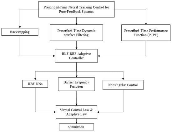
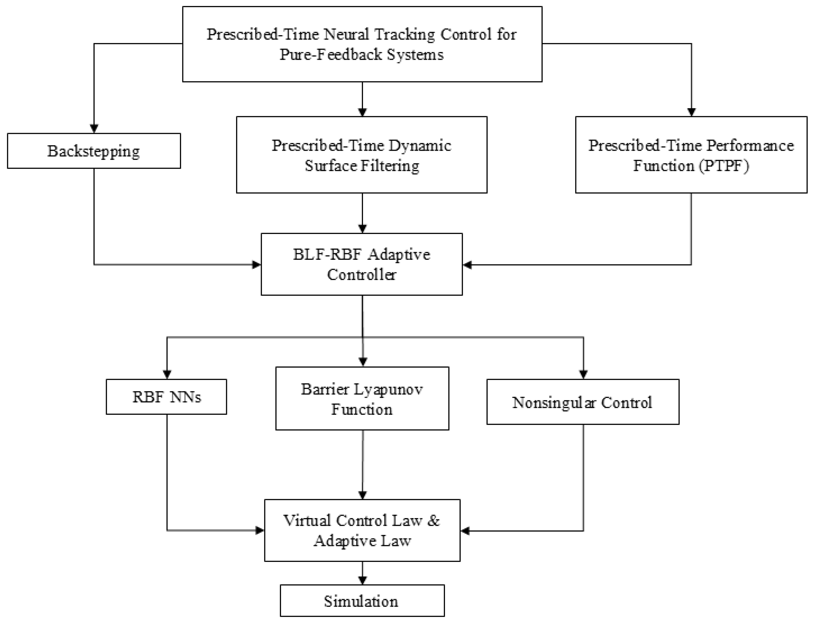
Figure 1 illustrates the overall framework of the proposed predefined-time adaptive neural control scheme. The recursive backstepping technique serves as the core design architecture, where the predefined-time command filter is adopted to overcome the complexity explosion issue of conventional backstepping. An improved barrier Lyapunov function is utilized to confine all state variables within their predefined bounds. Meanwhile, radial basis function neural networks (RBF NNs) are employed to approximate unknown nonlinear dynamics online, with adaptive laws designed to update weight estimates in real time. Finally, stacked Lyapunov functions are constructed to rigorously prove the predefined-time stability of the closed-loop system, and comparative simulation results are provided to further validate the effectiveness of the proposed control strategy. Table 1 compares the proposed scheme with [35] from four aspects: control objective, convergence time, dynamic surface filter, and singularity avoidance.

Figure 1. Research program.

Table 1. Comparison of technical features between the proposed scheme and the closely related work [35].

Technical Feature	Work in [35] (Liu et al., IEEE TNNLS, 2025)	Proposed Scheme
Control Objective	Prescribed performance control: ensures the tracking error evolves strictly within a predefined performance envelope.	Predefined-time stability: ensures the tracking error converges to a prescribed residual set within an arbitrarily user-assigned time $T_c$, independent of initial conditions.
Convergence Time	Depends on design parameters and initial conditions; cannot be explicitly and arbitrarily prescribed by the user a priori.	Explicitly assignable via the single parameter $T_c$ in Lemma 4; the settling time is uniform with respect to initial states.
Dynamic Surface Control	Employs a standard first-order low-pass filter.	Employs a predefined-time-dynamic surface filter, whose convergence is rigorously proven to occur within the same user-defined time $T_c$.
Singularity Avoidance in Control Laws	Uses standard regularization or simple saturation.	Develops a piecewise smooth function ${\delta }_i$, specifically designed to eliminate potential singularities caused by fractional-power terms in the virtual/actual control laws, while fully preserving the required predefined-time convergence.

2. Problem Formulation and Preliminaries

This section presents the system model and the necessary preliminaries and lemmas for controller design. The main symbols used in this paper are summarized in Table 2.

Table 2. Notations.

Symbol	Definition	Symbol	Definition
$x_i$	System state $(i=1,2,\dots ,n)$	$f_i(·)$	Unknown nonlinear function $(i=1,2,\dots ,n)$
${\overline{x}}_i$	Partial state vector $(i=1,2,\dots ,n)$	${\varphi }_i(·)$	Known nonlinear function $(i=1,2,\dots ,n)$
x	Full state vector	${\delta }_i$	Piecewise nonsingular auxiliary function $(i=1,2,\dots ,n)$
y	System output	${\sigma }_r,{\phi }_r$	Tunable parameters of PTPF
u	Actual control input	${\widehat{\theta }}_i$	Estimate of squared NN weight norm $(i=1,2,\dots ,n)$
$y_d$	Desired trajectory	${\tilde{\theta }}_i$	NN weight norm estimation error $(i=1,2,\dots ,n)$
$z_i$	Error variable $(i=1,2,\dots ,n)$	${\theta }_i$	Ideal squared NN weight norm $(i=1,2,\dots ,n)$
${\alpha }_i$	Virtual controller $(i=1,2,\dots ,n)$	${\pi }_{i,1},{\pi }_{i,2}$	Predefined-time convergence gain $(i=1,2,\dots ,n)$
${\xi }_i$	Compensation error $(i=1,2,\dots ,n)$	${\lambda }_i,{\mu }_i$	Dynamic surface filter gain $(i=2,3,\dots ,n)$
$g_i$	Filter output $(i=1,2,\dots ,n)$	$p_{r,f}$	Steady residual bound of PTPF
$d_i\left(t\right)$	External disturbance $(i=1,2,\dots ,n)$	$p_{r,0}$	Initial value of PTPF

Consider a class of nonlinear pure-feedback systems subject to state constraints, whose dynamics are given by [35]

$$\left\{\begin{array}{c}{\dot{x}}_i=f_i({\overline{x}}_i,x_{i+1})+{\varphi }_i\left({\overline{x}}_i\right)x_{i+1}+d_i\left(t\right)\hfill \\ {\dot{x}}_n=f_n\left(x\right)+{\varphi }_n\left(x\right)u+d_n\left(t\right)\hfill \\ y=x_1\hfill \end{array}\right.$$

(1)

In the system described above, $x_i$, u, y denote the state variables, control input, and system output, respectively, with ${\overline{x}}_i={[x_1,x_2,\dots ,x_i]}^T\in {\mathbb{R}}^i$ and $x={[x_1,\dots ,x_n]}^T\in {\mathbb{R}}^n$, whereas the smooth functions $f_i(·)$ are unknown, and $f_i({\overline{x}}_i,x_{i+1})$ exhibits a non-affine dependence on $x_{i+1}$, which preserves the pure-feedback nature of the system. The terms ${\varphi }_i\left({\overline{x}}_i\right)$ are known nonlinear functions satisfying ${\varphi }_i\left({\overline{x}}_i\right)\ne 0$, and ${\varphi }_i\left({\overline{x}}_i\right)x_{i+1}$ are explicitly separated affine terms from the non-affine dynamics. $d_i\left(t\right)$ are unknown external disturbances.

Assumption 1.

To guarantee the controllability of system (1), we assume that for $i=1,2,\dots ,n$ (with $x_{n+1}:=u$), the following inequality holds:

$${\displaystyle \frac{\partial f_i({\overline{x}}_i,x_{i+1})}{\partial x_{i+1}}}+{\varphi }_i\left({\overline{x}}_i\right)\ne 0,\forall ({\overline{x}}_i,x_{i+1})\in \Omega$$

(2)

where Ω is a bounded compact set of interest. This condition ensures that the virtual control variable $x_{i+1}$ (or the actual input u) has a non-vanishing regulating effect on the dynamics of $x_i$. In addition to Assumption 1, for the explicitly separated affine term, we assume that the known function ${\varphi }_i\left({\overline{x}}_i\right)$ is strictly nonzero and bounded away from zero on the compact set Ω, $\left|{\varphi }_i\left({\overline{x}}_i\right)\right|\ge {\varphi }_{i,min}>0$.

Remark 1.

In the special case $f_i({\overline{x}}_i,x_{i+1})=-{\varphi }_i\left({\overline{x}}_i\right)x_{i+1}$, the control term cancels completely and the subsystem reduces to ${\dot{x}}_i=d_i\left(t\right)$, so no controller can influence $x_i$, rendering the system uncontrollable in that channel; Assumption 1 excludes such degenerate cases. However, the condition may still fail locally in practice even when the system is not globally uncontrollable: (i) if $\partial f_i/\partial x_{i+1}=-{\varphi }_i\left({\overline{x}}_i\right)$ at isolated points, the effective gain vanishes and the backstepping control law becomes singular, causing performance degradation near those points; (ii) actuator nonlinearities such as dead-zone, saturation, or stall can drive the incremental gain $\partial f_i/\partial x_{i+1}$ to zero, so the effective gain may vanish even though ${\varphi }_i\left({\overline{x}}_i\right)\ne 0$; (iii) underactuated or singular configurations may temporarily prevent the virtual control $x_{i+1}$ from affecting $x_i$; and (iv) if the strict nonzero condition on ${\varphi }_i\left({\overline{x}}_i\right)$ were relaxed, its zeros could combine with the derivative term to produce zero effective gain. When the assumption fails locally, the designed controller may generate unbounded virtual signals or fail to stabilize the subsystem, so in practice one should restrict the operating region, employ switched or segmented control, or redesign the actuator to avoid such singularities. Thus, Assumption 1 defines the operating range over which the proposed method guarantees stability.

Lemma 1

([35,51]). The predefined-time performance function is a smooth function $\theta \left(t\right)$, such that $\theta \left(t\right)>0$, $\dot{\theta }\left(t\right)<0$, and $\theta \left(t\right)$ converges to ${\theta }_{T_p}>0$ at the prescribed time $T_p$ and remains constant thereafter, $\theta \left(t\right)={\theta }_{T_p},t\ge T_p$. Based on the above definition, the following PTPF $p_r\left(t\right)$ is adopted:

$$p_r\left(t\right)=\left\{\begin{array}{cc}{\left(p_{r,0}^{{\sigma }_r}-{\sigma }_r{\phi }_{r}t\right)}^{{\displaystyle \frac{1}{{\sigma }_r}}}+p_{r,f},\hfill & 0\le t<T_{r,p}\hfill \\ p_{r,f},\hfill & t\ge T_{r,p}\hfill \end{array}\right.$$

(3)

with $p_{r,0},{\sigma }_r,{\phi }_r$ and $p_{r,f}$ being positive constants to be chosen by the designer, and $T_{r,p}=p_{r,0}^{{\sigma }_r}/{\sigma }_r{\phi }_r$ being the prescribed settling time.

Lemma 2

([35]). Consider a system described by $\dot{s}=f\left(s\right)$, defined over an open region F that contains the origin. A barrier Lyapunov function $L\left(s\right)$ is defined as a continuous, scalar-valued, positive definite function on F, possessing continuous first-order partial derivatives throughout F. It must meet two conditions: (i) $L\left(s\right)$ diverges to infinity as s tends toward the boundary of F, and (ii) for every $t\ge 0$, the value of $L\left(s\right)$ along any trajectory of $\dot{s}=f\left(s\right)$ remains bounded above by a fixed constant $\alpha >0$.

Therefore, based on the above theorem, a barrier Lyapunov function incorporating the PTPF is adopted, as given below:

$$L_r=log\left({\displaystyle \frac{p_r^2}{p_r^2-z_r^2}}\right)$$

(4)

where $z_r$ is the error variable, and this function can ensure that $z_r$ is strictly confined within the prescribed bound $p_r$, thereby achieving safety constraints on the system states.

Lemma 3

([52]). In this work, the radial basis function neural network (RBF NN) is adopted to approximate the continuous function $F(\Xi ):{\mathbb{R}}^n\to \mathbb{R}$. There exists an RBF NN satisfying

$$F(\Xi )=h^{*T}S(\Xi )$$

(5)

where $\Xi \in {\Omega }_{\Xi }\subset {\mathbb{R}}^l$, is the input vector, $h={[h_1,\dots ,h_b]}^T\in {\mathbb{R}}^b(b>1)$ is the weight vector, and $S(\Xi )={[S_1(\Xi ),\dots ,S_b(\Xi )]}^T$ denotes the basis function vector; each component $S_i(\Xi )$ is a Gaussian function given by

$$S_i(\Xi )=exp\left[-{\displaystyle \frac{{(\Xi -{\psi }_i)}^T(\Xi -{\psi }_i)}{q_i^2}}\right]$$

(6)

with ${\psi }_i={[{\psi }_{i1},{\psi }_{i2},\dots ,{\psi }_{il}]}^T$ and $q_i$ being the center and width of the receptive field, respectively. As stated in, this RBF NN structure can approximate any continuous function on the compact set ${\Omega }_{\Xi }$, yielding

$$F(\Xi )=h^{*T}S(\Xi )+q(\Xi ),\left|q(\Xi )\right|\le \epsilon$$

(7)

where $q(\Xi )$ is the approximation error, and the ideal weight $h^{*}$ is defined as

$$h^{*}=arg\underset{h\in {\mathbb{R}}^b}{min}\left\{\underset{\Xi \in {\Omega }_{\Xi }}{sup}\left|F(\Xi )-h^{T}S(\Xi )\right|\right\}$$

(8)

The control objectives of this paper are threefold: (i) the output y tracks the desired signal $y_d$; (ii) the tracking error $z_1$ converges to a preset precision within the predefined time $T_c$ and remains within the prescribed bound $|z_1|<p_1$ for all $t>0$; and (iii) all signals in the considered system (1) are guaranteed to be predefined-time bounded.

Remark 2.

The RBF neural network is adopted in this work due to its linearly parameterized structure, which facilitates a rigorous Lyapunov-based stability analysis, an essential requirement for the proposed predefined-time control framework, and due to its low computational cost, as only scalar adaptive parameters need to be updated online. Alternative recurrent architectures, such as echo state networks (ESNs), typically require offline training and lack tractable stability analysis due to their complex reservoir dynamics, making them less suitable for the real-time adaptive control setting considered here. Nevertheless, we acknowledge that the approximation capability of RBF networks depends on the proper selection of centers and widths, and their performance may degrade for highly time-varying nonlinearities. For the class of systems and disturbances studied in this paper, however, the adopted RBF configuration proves sufficient to achieve satisfactory tracking performance.

Definition 1

([53]). Consider a nonlinear system $\dot{x}=f(x,t)$. If for any given positive constants $\tau >0$ and a user-specified time $T_c>0$, the system trajectory satisfies $\parallel x\left(t\right)\parallel \le \tau ,\forall t\ge T_c$, then the system is said to be practically stable within the predefined time $T_c$.

Lemma 4

([53]). It is supposed that there exists a continuous positive definite function $V\left(x\right)$:

$$\dot{V}\le -{\displaystyle \frac{\pi }{r{T}_c}}\left(V^{1+{\displaystyle \frac{r}{2}}}+V^{1-{\displaystyle \frac{r}{2}}}\right)+\eta$$

(9)

where $T_c>0$, $\eta >0$, $r\in (0,1)$ and $\eta >0$ is a constant. Then, the system is practically predefined-time-stable, and the convergence time is bounded by $\sqrt{2}{T}_c$.

Lemma 5

([53]). For any ${\varphi }_1\in \mathbb{R}$, ${\varphi }_2\in \mathbb{R}$, and positive constants $\omega >0$, $\rho >0$ and $\tau >0$, the following inequality holds:

$$|{\varphi }_1{|}^{\omega }|{\varphi }_2{|}^{\rho }\le {\displaystyle \frac{\omega }{\omega +\rho }}\tau |{\varphi }_1{|}^{\omega +\rho }+{\displaystyle \frac{\rho }{\omega +\rho }}{\tau }^{-{\displaystyle \frac{\omega }{\rho }}}{|{\varphi }_2|}^{\omega +\rho }.$$

(10)

In addition, a predefined-time filter will be introduced in the next section to facilitate the backstepping design, whose detailed construction is given in the controller design phase.

Lemma 6

([54]). For any $x_i\in {\mathbb{R}}_{+}$, $i=1,2,\dots ,n$, and any constants $0<p\le 1$ and $q>1$, the following inequalities hold:

$$\begin{array}{c}\hfill {\left({\displaystyle \sum _{i=1}^n}{x}_i\right)}^p\le {\displaystyle \sum _{i=1}^n}{x}_i^p\le n^{1-p}{\left({\displaystyle \sum _{i=1}^n}{x}_i\right)}^p\end{array}$$

(11)

$$\begin{array}{c}\hfill n^{1-q}{\left({\displaystyle \sum _{i=1}^n}{x}_i\right)}^q\le {\displaystyle \sum _{i=1}^n}{x}_i^q\le {\left({\displaystyle \sum _{i=1}^n}{x}_i\right)}^q\end{array}$$

(12)

Assumption 2.

The reference signal $y_d\left(t\right)$ and its derivatives ${\dot{y}}_d\left(t\right)$ and ${\ddot{y}}_d\left(t\right)$ are continuous and bounded.

Assumption 3.

The system states $x_i$ ($i=1,2,\dots ,n$) are required to strictly satisfy the physical constraints $|x_i|<k_i,i=1,2,\dots ,n$, where $k_i>0$ are known constants. In cases where only a subset of states is physically constrained, the corresponding $k_i$ for the unconstrained states can be chosen to be sufficiently large so that the constraints are inactive during operation.

Assumption 4.

The lumped unknown disturbances $d_i\left(t\right)$, $i=1,2,\dots ,n$, are bounded. Specifically, there exist positive constants ${\overline{d}}_i$ such that $|d_i\left(t\right)|\le {\overline{d}}_i$, $i=1,2,\dots ,n$, for all $t\ge 0$.

3. Predefined-Time Controller Design

To facilitate the subsequent controller design, several coordinate transformations are introduced, and an adaptive NN backstepping controller is constructed to achieve tracking performance and signal boundedness. Meanwhile, a predefined-time filter is employed to overcome the complexity explosion. The detailed design is conducted in several steps and is based on the following coordinate transformations:

$$\left\{\begin{array}{c}{z}_1=x_1-y_d\hfill \\ z_i=x_i-g_i\hfill \end{array}\right.$$

(13)

where $z_1$ denotes the tracking error with respect to the reference trajectory $y_d$, and $z_i$ and $g_i$ with $i=2,3,\dots ,n$ stand for the tracking error and output of the filter, respectively.

Remark 3.

It should be noted that the command filter inevitably introduces filtering errors, which makes high-precision tracking more challenging. To compensate for these errors, the filtering error signal ${\xi }_i$ defined in (14) will serve as the compensation signal and will be explicitly incorporated into the virtual control law in the subsequent design steps to cancel out the filtering error effect, thereby improving the tracking accuracy.

Then, the compensated tracking error signals are defined as follows:

$${\xi }_i=g_i-{\alpha }_{i-1}$$

(14)

The signal $g_i$ ($2\le i\le n-1$) generated by the following predefined-time-dynamic surface filter is employed to estimate the virtual control law ${\alpha }_{i-1}$. To this end, an improved predefined-time filter is introduced as follows:

$$\left\{\begin{array}{c}{\dot{g}}_i=-{\lambda }_i{\xi }_i^{r+1}{\displaystyle \frac{1}{r{T}_c}}-{\mu }_i{\xi }_i^{1-r}{\displaystyle \frac{1}{r{T}_c}}-{\xi }_i,\hfill \\ g_i\left(0\right)={\alpha }_{i-1}\left(0\right)\hfill \end{array}\right.$$

(15)

where ${\lambda }_i>0$ and ${\mu }_i>0$ are design parameters, $T_c>0$ and $0<r<1$ are design constants.

3.1. Controller Design Procedure

Step 1: With the aid of (1), (13) and (14), one can obtain

$$\begin{array}{cc}\hfill {\dot{z}}_1& ={\dot{x}}_1-{\dot{y}}_d\hfill \\ \hfill & =f_1+{\varphi }_1{x}_2+d_1-{\dot{y}}_d\hfill \\ \hfill & =f_1+{\varphi }_1{z}_2+{\varphi }_1{\xi }_2+{\varphi }_1{\alpha }_1+d_1-{\dot{y}}_d\hfill \end{array}$$

(16)

Let the parameter estimation error be defined as ${\tilde{\theta }}_1={\theta }_1-{\widehat{\theta }}_1.$ Choose a Lyapunov function candidate as follows:

$$V_1={\displaystyle \frac{1}{2}}log\left({\displaystyle \frac{p_1^2}{p_1^2-z_1^2}}\right)+{\displaystyle \frac{1}{2}}{\tilde{\theta }}_1^2$$

(17)

Taking the time derivative of $V_1$, one can obtain

$$\begin{array}{cc}\hfill {\dot{V}}_1& ={\vartheta }_1{\dot{z}}_1-{\vartheta }_1{\displaystyle \frac{{\dot{p}}_1{z}_1}{p_1}}-{\tilde{\theta }}_1{\dot{\widehat{\theta }}}_1\hfill \\ \hfill & ={\vartheta }_1(f_1+{\varphi }_1{z}_2+{\varphi }_1{\xi }_2+{\varphi }_1{\alpha }_1+d_1-{\dot{y}}_d)-{\vartheta }_1{\displaystyle \frac{{\dot{p}}_1{z}_1}{p_1}}-{\tilde{\theta }}_1{\dot{\widehat{\theta }}}_1\hfill \end{array}$$

(18)

where ${\vartheta }_1={\displaystyle \frac{z_1}{p_1^2-z_1^2}}$, and $F_1\left({\Xi }_1\right)=f_1({\overline{x}}_1,x_2)+d_1\left(t\right)$.

The unknown function $f_1\left(x\right)$ renders the direct construction of the virtual control signal ${\alpha }_1$ impossible. To address this issue, an RBF NN is introduced to approximate $f_1\left(x\right)$. Hence, for any prescribed ${\epsilon }_1>0$,

$$F_1\left({\Xi }_1\right)=h_1^{*T}{S}_1\left({\Xi }_1\right)+q_1\left({\Xi }_1\right),\left|q_1\left({\Xi }_1\right)\right|\le {\epsilon }_1$$

(19)

where ${\Xi }_1={\left[x_1,x_2\right]}^T$, and $q_1\left({\Xi }_1\right)$ denotes the approximation error.

Let ${\theta }_1={∥h_1^{*}∥}^2$, let ${\widehat{\theta }}_1$ be the estimate of ${\theta }_1$, and define the estimation error as ${\tilde{\theta }}_1={\theta }_1-{\widehat{\theta }}_1$. For any constant $a_1>0$, by invoking Young’s inequality, we have

$$\begin{array}{cc}\hfill {\vartheta }_1{F}_1\left({\Xi }_1\right)& ={\vartheta }_1{h}_1^{*T}{S}_1\left({\Xi }_1\right)+{\vartheta }_1{q}_1\left({\Xi }_1\right)\hfill \\ \hfill & \le {\displaystyle \frac{1}{2}}{\theta }_1{S}_1^T{S}_1+{\displaystyle \frac{1}{2}}{\vartheta }_1^2+{\displaystyle \frac{1}{2a_1}}{\vartheta }_1^2+{\displaystyle \frac{a_1}{2}}{\epsilon }_1^2\hfill \end{array}$$

(20)

Substituting (20) into (18) yields

$$\begin{array}{cc}\hfill {\dot{V}}_1& \le {\displaystyle \frac{1}{2}}{\theta }_1{S}_1^T{S}_1+\left({\displaystyle \frac{1}{2}}+{\displaystyle \frac{1}{2a_1}}\right){\vartheta }_1^2+{\displaystyle \frac{a_1}{2}}{\epsilon }_1^2\hfill \\ \hfill & +{\vartheta }_1{\varphi }_1{z}_2+{\vartheta }_1{\varphi }_1{\xi }_2+{\vartheta }_1{\varphi }_1{\alpha }_1-{\vartheta }_1{\dot{y}}_d-{\vartheta }_1{\displaystyle \frac{{\dot{p}}_1{z}_1}{p_1}}-{\tilde{\theta }}_1{\dot{\widehat{\theta }}}_1.\hfill \end{array}$$

(21)

To avoid the division-by-zero singularity caused by the RBF-NN compensation terms, the smooth regularized inverse function ${\mathcal{I}}_{{\rho }_1}\left({\vartheta }_1\right)={\displaystyle \frac{{\vartheta }_1}{{\vartheta }_1^2+{\rho }_1^2}}$ is introduced, where ${\rho }_1>0$ is a sufficiently small design constant. This function is globally continuous and bounded, satisfying ${\mathcal{I}}_{{\rho }_1}\left(0\right)=0$ and $|{\mathcal{I}}_{{\rho }_1}\left({\vartheta }_1\right)|\le 1/\left(2{\rho }_1\right)$. To stabilize the subsystem in predefined-time, we can now design the predefined-time virtual controller ${\alpha }_1$ as

$$\begin{array}{c}\hfill \begin{array}{cc}\hfill {\alpha }_1& ={\displaystyle \frac{1}{{\varphi }_1}}\left[{\displaystyle \frac{{\dot{p}}_1{z}_1}{p_1}}+{\dot{y}}_d-{\varphi }_1{z}_2-{\displaystyle \frac{{\pi }_{1,1}}{r{T}_c}}{\left({\displaystyle \frac{1}{2}}\right)}^{1+{\displaystyle \frac{r}{2}}}{\vartheta }_1^{r+1}\right.\hfill \\ \hfill & -{\displaystyle \frac{{\pi }_{1,2}}{r{T}_c}}{\left({\displaystyle \frac{1}{2}}\right)}^{1-{\displaystyle \frac{r}{2}}}{\delta }_1-{\displaystyle \frac{1}{2}}{\vartheta }_1-{\displaystyle \frac{1}{2}}{a}_1{\epsilon }_1^2{\mathcal{I}}_{{\rho }_1}\left({\vartheta }_1\right)\hfill \\ \hfill & \left.-{\displaystyle \frac{1}{2a_1}}{\vartheta }_1-{\displaystyle \frac{1}{2}}{\widehat{\theta }}_1{S}_1^{\mathrm{T}}{S}_1{\mathcal{I}}_{{\rho }_1}\left({\vartheta }_1\right)\right]\hfill \end{array}\end{array}$$

(22)

Define the residual term induced by regularization as

$$\begin{array}{c}\hfill \begin{array}{cc}\hfill R_{{\rho }_1}& ={\displaystyle \frac{1}{2}}\left({\widehat{\theta }}_1{S}_1^{\mathrm{T}}{S}_1+a_1{\epsilon }_1^2\right)-{\displaystyle \frac{1}{2}}\left({\widehat{\theta }}_1{S}_1^{\mathrm{T}}{S}_1+a_1{\epsilon }_1^2\right){\displaystyle \frac{{\vartheta }_1^2}{{\vartheta }_1^2+{\rho }_1^2}}\hfill \\ \hfill & ={\displaystyle \frac{{\rho }_1^2}{2\left({\vartheta }_1^2+{\rho }_1^2\right)}}\left({\widehat{\theta }}_1{S}_1^{\mathrm{T}}{S}_1+a_1{\epsilon }_1^2\right)\hfill \end{array}\end{array}$$

(23)

where ${\pi }_{1,1}$, ${\pi }_{1,2}$, $T_c$ are positive design constants and $0<r<1$, ${\delta }_1$ can be defined as

$${\delta }_1=\left\{\begin{array}{cc}{\vartheta }_1^{1-r},\hfill & |{\vartheta }_1|\ge {\Omega }_1>0\hfill \\ {\displaystyle {\displaystyle \sum _{j=1}^{n+1}}{\ell }_j{\vartheta }_1^{2j-1}{\left({\Omega }_1^2\right)}^{-j+1-\frac{r}{2}},}\hfill & |{\vartheta }_1|<{\Omega }_1\hfill \end{array}\right.$$

(24)

where ${\Omega }_1>0$ is a small constant, and the coefficients ${\ell }_j$ are determined by the smoothness conditions at the switching point $|{\vartheta }_1|={\Omega }_1$ as described in the following linear system.

$$\begin{array}{cc}\hfill {\ell }_1+{\ell }_2+\dots +{\ell }_n+{\ell }_{n+1}& ={\beta }_1,\hfill \\ \hfill {\ell }_1+3{\ell }_2+\dots +(2n-1){\ell }_n+(2n+1){\ell }_{n+1}& ={\beta }_2,\hfill \\ \hfill 0{\ell }_1+6{\ell }_2+\dots +(2n-1)(2n-2){\ell }_n+(2n+1)\left(2n\right){\ell }_{n+1}& ={\beta }_3,\hfill \\ \hfill & ⋮\hfill \\ \hfill {\displaystyle \prod _{k=0}^{n-1}}(1-k){\ell }_1+\dots +{\displaystyle \prod _{k=0}^{n-1}}(2n+1-k){\ell }_{n+1}& ={\beta }_{n+1},\hfill \end{array}$$

(25)

where ${\beta }_1=1,{\beta }_2=1-r,{\beta }_3=(1-r)(-r),\dots ,{\beta }_{n+1}={\displaystyle \prod _{m=0}^{n-1}}(1-r-m)$.

Remark 4.

For the case $n=2$ considered in this paper, the coefficients obtained from the linear system are ${\ell }_1=1+{\displaystyle \frac{r^2+6r}{8}},{\ell }_2=-{\displaystyle \frac{r^2+4r}{4}},{\ell }_3={\displaystyle \frac{r(r+2)}{8}}.$ We now explicitly verify the continuity and differentiability of ${\delta }_1$ at the switching boundary $|{\vartheta }_1|={\Omega }_1$. In terms of symmetry, it suffices to examine ${\vartheta }_1\ge 0$. As ${\vartheta }_1\to {\Omega }_1^{-}$, the internal polynomial expression gives ${lim}_{{\vartheta }_1\to {\Omega }_1^{-}}{\delta }_1=({\ell }_1+{\ell }_2+{\ell }_3){\Omega }_1^{1-r}={\Omega }_1^{1-r},$ where the last equality follows from the first equation of the linear system, i.e., ${\ell }_1+{\ell }_2+{\ell }_3={\beta }_1=1$. This coincides with the external value ${\delta }_1{|}_{{\vartheta }_1={\Omega }_1^{+}}={\Omega }_1^{1-r}$, so ${\delta }_1$ is continuous at the switching point. Furthermore, differentiating the internal polynomial with respect to ${\vartheta }_1$ and taking the left-hand limit yields ${lim}_{{\vartheta }_1\to {\Omega }_1^{-}}{\displaystyle \frac{\partial {\delta }_1}{\partial {\vartheta }_1}}=({\ell }_1+3{\ell }_2+5{\ell }_3){\Omega }_1^{-r}=(1-r){\Omega }_1^{-r},$ where the second equation of the linear system, ${\ell }_1+3{\ell }_2+5{\ell }_3={\beta }_2=1-r$, has been used. This equals the derivative of the external function ${\vartheta }_1^{1-r}$ evaluated at ${\vartheta }_1={\Omega }_1$, namely $(1-r){\Omega }_1^{-r}$. Therefore, ${\delta }_1$ is $C^1$-smooth at the switching boundary. Higher-order differentiability is not required for the subsequent control design, and imposing it would unnecessarily overconstrain the coefficient selection.

Remark 5.

The constant ${\Omega }_1>0$ defines the boundary of the smoothing region for ${\delta }_1$. Its choice directly affects the control smoothness, convergence rate, and steady-state accuracy. Recall that outside the boundary layer ($|{\vartheta }_1|\ge {\Omega }_1$), the original terminal term ${\vartheta }_1^{1-r}$ is used. This term provides fast convergence near ${\vartheta }_1=0$ because its derivative $(1-r){\vartheta }_1^{-r}$ tends to infinity as ${\vartheta }_1\to 0$. However, this infinite derivative also causes severe control chattering and numerical singularities. Inside the boundary layer ($|{\vartheta }_1|<{\Omega }_1$), the polynomial replaces the terminal term to remove this singularity, at the cost of slowing down the convergence near the origin. Therefore, a larger ${\Omega }_1$ enlarges the smoothing interval, yielding smoother control signals and better numerical robustness, but inevitably enlarges the steady-state tracking error bound and reduces the convergence rate. Conversely, a smaller ${\Omega }_1$ preserves the terminal convergence and achieves higher steady-state precision, but may excite high-frequency oscillations and cause numerical ill-conditioning.

In practice, ${\Omega }_1$ should be chosen according to the following guidelines: (i) It should be small enough to satisfy the desired steady-state error tolerance. (ii) It should be large enough to avoid chattering caused by measurement noise and finite sampling time. As a practical initial guideline, ${\Omega }_1$ can be chosen slightly larger than the amplitude of the steady-state measurement noise (e.g., in normalized systems or with standard sensors, a value of the order ${10}^{-2}\sim {10}^{-3}$ can serve as a starting point). (iii)If both high transient robustness and high steady-state precision are required, a time-varying ${\Omega }_1\left(t\right)$ can be adopted: start with a relatively large value to suppress chattering during the initial transient, then exponentially decrease to a very small final value to recover the terminal convergence near equilibrium.This inherent trade-off is also illustrated in the simulation results, where different fixed values of ${\Omega }_1$ are compared.

When $|{\vartheta }_1|\ge {\Omega }_1$, ${\dot{V}}_1$ is given by

$${\dot{V}}_1\le -{\displaystyle \frac{{\pi }_{1,1}}{r{T}_c}}{\left({\displaystyle \frac{1}{2}}\right)}^{1+{\displaystyle \frac{r}{2}}}{\vartheta }_1^{2+r}-{\displaystyle \frac{{\pi }_{1,2}}{r{T}_c}}{\left({\displaystyle \frac{1}{2}}\right)}^{1-{\displaystyle \frac{r}{2}}}{\vartheta }_1^{2-r}+{\vartheta }_1{\varphi }_1{\xi }_2-{\tilde{\theta }}_1{\dot{\widehat{\theta }}}_1+{\displaystyle \frac{1}{2}}{\tilde{\theta }}_1{S}_1^T{S}_1+R_{{\rho }_1}$$

(26)

and the adaptation law as

$${\dot{\widehat{\theta }}}_1={\displaystyle \frac{1}{2}}{S}_1^T{S}_1-c_{1,1}{\widehat{\theta }}_1$$

(27)

Noticing that $c_{1,1}$ is a positive constant and using the inequality ${\tilde{\theta }}_1{\widehat{\theta }}_1={\tilde{\theta }}_1({\theta }_1-{\tilde{\theta }}_1)\le {\displaystyle \frac{1}{2}}\left({\theta }_1^2-{\tilde{\theta }}_1^2\right)$, we have

$$\begin{array}{cc}\hfill c_{1,1}{\tilde{\theta }}_1{\widehat{\theta }}_1& =c_{1,1}{\tilde{\theta }}_1\left({\theta }_1-{\tilde{\theta }}_1\right)\hfill \\ \hfill & \le {\displaystyle \frac{c_{1,1}}{2}}\left({\theta }_1^2-{\tilde{\theta }}_1^2\right)\hfill \end{array}$$

(28)

Combining (27) and (28) with (26), ${\dot{V}}_1$ can be expressed as

$${\dot{V}}_1\le -{\displaystyle \frac{{\pi }_{1,1}}{r{T}_c}}{\left({\displaystyle \frac{1}{2}}\right)}^{1+{\displaystyle \frac{r}{2}}}{\vartheta }_1^{2+r}-{\displaystyle \frac{{\pi }_{1,2}}{r{T}_c}}{\left({\displaystyle \frac{1}{2}}\right)}^{1-{\displaystyle \frac{r}{2}}}{\vartheta }_1^{2-r}+{\vartheta }_1{\varphi }_1{\xi }_2+{\displaystyle \frac{c_{1,1}}{2}}\left({\theta }_1^2-{\tilde{\theta }}_1^2\right)+R_{{\rho }_1}$$

(29)

When $|{\vartheta }_1|<{\Omega }_1$, ${\dot{V}}_1$ is given by

$$\begin{array}{cc}\hfill {\dot{V}}_1& \le -{\displaystyle \frac{{\pi }_{1,1}}{r{T}_c}}{\left({\displaystyle \frac{1}{2}}\right)}^{1+{\displaystyle \frac{r}{2}}}{\vartheta }_1^{2+r}+{\vartheta }_1{\varphi }_1{\xi }_2-{\displaystyle \frac{{\pi }_{1,2}}{r{T}_c}}{\left({\displaystyle \frac{1}{2}}\right)}^{1-{\displaystyle \frac{r}{2}}}{\displaystyle \sum _{j=1}^{n+1}}{\ell }_j{\left({\vartheta }_1^2\right)}^j{\left({\Omega }_1^2\right)}^{-j+1-{\displaystyle \frac{r}{2}}}\hfill \\ \hfill & -{\tilde{\theta }}_1{\dot{\widehat{\theta }}}_1+{\displaystyle \frac{1}{2}}{\tilde{\theta }}_1{S}_1^T{S}_1+R_{{\rho }_1}\hfill \end{array}$$

(30)

and the adaptation law as

$${\dot{\widehat{\theta }}}_1={\displaystyle \frac{1}{2}}{S}_1^T{S}_1-c_{1,2}{\widehat{\theta }}_1$$

(31)

Noticing that $c_{1,2}$ is a positive constant and using the inequality ${\tilde{\theta }}_1{\widehat{\theta }}_1={\tilde{\theta }}_1({\theta }_1-{\tilde{\theta }}_1)\le {\displaystyle \frac{1}{2}}\left({\theta }_1^2-{\tilde{\theta }}_1^2\right)$, we have

$$\begin{array}{cc}\hfill c_{1,2}{\tilde{\theta }}_1{\widehat{\theta }}_1& =c_{1,2}{\tilde{\theta }}_1\left({\theta }_1-{\tilde{\theta }}_1\right)\hfill \\ \hfill & \le {\displaystyle \frac{c_{1,2}}{2}}\left({\theta }_1^2-{\tilde{\theta }}_1^2\right)\hfill \end{array}$$

(32)

Combining (31) and (32) with (30), ${\dot{V}}_1$ can be expressed as

$$\begin{array}{cc}\hfill {\dot{V}}_1& \le -{\displaystyle \frac{{\pi }_{1,1}}{r{T}_c}}{\left({\displaystyle \frac{1}{2}}\right)}^{1+{\displaystyle \frac{r}{2}}}{\vartheta }_1^{2+r}+{\vartheta }_1{\varphi }_1{\xi }_2\hfill \\ \hfill & +{\displaystyle \frac{c_{1,2}}{2}}\left({\theta }_1^2-{\tilde{\theta }}_1^2\right)-{\displaystyle \frac{{\pi }_{1,2}}{r{T}_c}}{\left({\displaystyle \frac{1}{2}}\right)}^{1-{\displaystyle \frac{r}{2}}}{\displaystyle \sum _{j=1}^{n+1}}{\ell }_j{\left({\vartheta }_1^2\right)}^j{\left({\Omega }_1^2\right)}^{-j+1-{\displaystyle \frac{r}{2}}}+R_{{\rho }_1}\hfill \end{array}$$

(33)

Let $A={\displaystyle \frac{{\pi }_{1,2}}{r{T}_c}}{\left({\displaystyle \frac{1}{2}}\right)}^{1-{\displaystyle \frac{r}{2}}}$, and $x_j={\left({\displaystyle \frac{{\vartheta }_1^2}{{\Omega }_1^2}}\right)}^{j-1+{\displaystyle \frac{r}{2}}}$. Then, the last term is rewritten as

$$\begin{array}{cc}\hfill & -{\displaystyle \frac{{\pi }_{1,2}}{r{T}_c}}{\left({\displaystyle \frac{1}{2}}\right)}^{1-{\displaystyle \frac{r}{2}}}{\displaystyle \sum _{j=1}^{n+1}}{\ell }_j{\left({\vartheta }_1^2\right)}^j{\left({\Omega }_1^2\right)}^{-j+1-{\displaystyle \frac{r}{2}}}\hfill \\ \hfill =& -A{\vartheta }_1^{2-r}{\displaystyle \sum _{j=1}^{n+1}}{\ell }_j{x}_j\hfill \end{array}$$

(34)

Since $|{\vartheta }_1|<{\Omega }_1$, we get $0<x_j<1$. Thus

$$\left|{\displaystyle \sum _{j=1}^{n+1}}{\ell }_j{x}_j\right|\le {\displaystyle \sum _{j=1}^{n+1}}|{\ell }_j|x_j\le {\displaystyle \sum _{j=1}^{n+1}}\left|{\ell }_j\right|$$

(35)

$$-A{\vartheta }_1^{2-r}{\displaystyle \sum _{j=1}^{n+1}}{\ell }_j{x}_j=-A{\vartheta }_1^{2-r}+A{\vartheta }_1^{2-r}\left(1-{\displaystyle \sum _{j=1}^{n+1}}{\ell }_j{x}_j\right)$$

(36)

Since $0<2-r$, we have

$$A{\vartheta }_1^{2-r}\left(1-{\displaystyle \sum _{j=1}^{n+1}}{\ell }_j{x}_j\right)\le A{\Omega }_1^{2-r}\left|1-{\displaystyle \sum _{j=1}^{n+1}}{\ell }_j{x}_j\right|\le A{\Omega }_1^{2-r}\left(1+{\displaystyle \sum _{j=1}^{n+1}}\left|{\ell }_j\right|\right)$$

(37)

Therefore

$$-A{\vartheta }_1^{2-r}{\displaystyle \sum _{j=1}^{n+1}}{\ell }_j{x}_j\le -A{\vartheta }_1^{2-r}+A{\Omega }_1^{2-r}\left(1+{\displaystyle \sum _{j=1}^{n+1}}\left|{\ell }_j\right|\right)$$

(38)

Combining (38) with (33), ${\dot{V}}_1$ can be expressed as

$$\begin{array}{cc}\hfill {\dot{V}}_1\le & -{\displaystyle \frac{{\pi }_{1,1}}{r{T}_c}}{\left({\displaystyle \frac{1}{2}}\right)}^{1+{\displaystyle \frac{r}{2}}}{\vartheta }_1^{2+r}+{\vartheta }_1{\varphi }_1{\xi }_2+{\displaystyle \frac{c_{1,2}}{2}}\left({\theta }_1^2-{\tilde{\theta }}_1^2\right)\hfill \\ \hfill & -A{\vartheta }_1^{2-r}+A{\Omega }_1^{2-r}\left(1+{\displaystyle \sum _{j=1}^{n+1}}\left|{\ell }_j\right|\right)+R_{{\rho }_1}\hfill \end{array}$$

(39)

From the above analysis, it is evident that for the case $|{\vartheta }_1|<{\Omega }_1$, inequality (39) introduces an additional bounded constant term $A{\Omega }_1^{2-r}\left(1+{\sum }_{j=1}^{n+1}\left|{\ell }_j\right|\right)$ compared with (29). In addition, since ${\vartheta }_1^2\ge 0$, we have ${\displaystyle \frac{{\rho }_1^2}{{\vartheta }_1^2+{\rho }_1^2}}\le 1$, and the estimated weight ${\widehat{\theta }}_1$ and tracking error ${\epsilon }_1$ are bounded in the closed-loop system. It can be concluded that the residual term $R_{{\rho }_1}$ is uniformly bounded. Hence, there exists an unknown positive constant ${\overline{R}}_1$ such that $|R_{{\rho }_1}|\le {\overline{R}}_1.$ To facilitate a unified stability analysis and avoid repetitive derivations, we define a positive constant ${\eta }_1={\displaystyle \frac{c_1}{2}}{\theta }_1^2+A{\Omega }_1^{2-r}\left(1+{\sum }_{j=1}^{n+1}\left|{\ell }_j\right|\right)+{\overline{R}}_1$ (where $c_1=c_{1,1}=c_{1,2}$ is selected for notational simplicity). Consequently, both cases can be compactly bounded by the following unified inequality:

$${\dot{V}}_1\le -{\displaystyle \frac{{\pi }_{1,1}}{r{T}_c}}{\left({\displaystyle \frac{1}{2}}\right)}^{1+{\displaystyle \frac{r}{2}}}{\vartheta }_1^{2+r}-{\displaystyle \frac{{\pi }_{1,2}}{r{T}_c}}{\left({\displaystyle \frac{1}{2}}\right)}^{1-{\displaystyle \frac{r}{2}}}{\vartheta }_1^{2-r}+{\vartheta }_1{\varphi }_1{\xi }_2-{\displaystyle \frac{c_1}{2}}{\tilde{\theta }}_1^2+{\eta }_1.$$

(40)

Step i ($2\le i\le n-1$): With the aid of (1), (13) and (14), one can get

$$\begin{array}{cc}\hfill {\dot{z}}_i& ={\dot{x}}_i-{\dot{g}}_i\hfill \\ \hfill & =f_i+{\varphi }_i{x}_{i+1}+d_i-{\dot{g}}_i\hfill \\ \hfill & =f_i+{\varphi }_i{z}_{i+1}+{\varphi }_i{\xi }_{i+1}+{\varphi }_i{\alpha }_i+d_i-{\dot{g}}_i\hfill \end{array}$$

(41)

Combining (15) with (14), ${\dot{\xi }}_i$ can be expressed as

$${\dot{\xi }}_i={\dot{g}}_i-{\dot{\alpha }}_{i-1}=-{\displaystyle \frac{{\lambda }_i{\xi }_i^{r+1}}{r{T}_c}}-{\displaystyle \frac{{\mu }_i{\xi }_i^{1-r}}{r{T}_c}}-{\xi }_i-{\dot{\alpha }}_{i-1}$$

(42)

Choose a Lyapunov function candidate as

$$V_i=V_{i-1}+{\displaystyle \frac{1}{2}}log\left({\displaystyle \frac{p_i^2}{p_i^2-z_i^2}}\right)+{\displaystyle \frac{1}{2}}{\tilde{\theta }}_i^2+{\displaystyle \frac{1}{2}}{\xi }_i^2$$

(43)

Taking the time derivative of $V_i$, one can get

$$\begin{array}{cc}\hfill {\dot{V}}_i& ={\dot{V}}_{i-1}+{\vartheta }_i{\dot{z}}_i-{\vartheta }_i{\displaystyle \frac{{\dot{p}}_i{z}_i}{p_i}}-{\tilde{\theta }}_i{\dot{\widehat{\theta }}}_i+{\xi }_i{\dot{\xi }}_i\hfill \\ \hfill & ={\dot{V}}_{i-1}+{\vartheta }_i\left(f_i+{\varphi }_i{z}_{i+1}+{\varphi }_i{\xi }_{i+1}+{\varphi }_i{\alpha }_i+d_i-{\dot{g}}_i\right)-{\vartheta }_i{\displaystyle \frac{{\dot{p}}_i{z}_i}{p_i}}\hfill \\ \hfill & -{\tilde{\theta }}_i{\dot{\widehat{\theta }}}_i+{\xi }_i\left[-{\displaystyle \frac{{\lambda }_i{\xi }_i^{r+1}}{r{T}_c}}-{\displaystyle \frac{{\mu }_i{\xi }_i^{1-r}}{r{T}_c}}-{\xi }_i-{\dot{\alpha }}_{i-1}\right]\hfill \end{array}$$

(44)

where ${\vartheta }_i={\displaystyle \frac{z_i}{p_i^2-z_i^2}}$, and $F_i\left({\Xi }_i\right)=f_i({\overline{x}}_i,x_{i+1})+d_i\left(t\right)$.

The unknown function $f_i\left(x\right)$ renders the direct construction of the virtual control signal ${\alpha }_i$ impossible. To address this issue, an RBF NN is introduced to approximate $f_i\left(x\right)$. Hence, for any prescribed ${\epsilon }_i>0$,

$$F_i\left({\Xi }_i\right)=h_i^{*T}{S}_i\left({\Xi }_i\right)+q_i\left({\Xi }_i\right),\left|q_i\left({\Xi }_i\right)\right|\le {\epsilon }_i$$

(45)

where ${\Xi }_i={\left[x_1,\dots ,x_{i+1}\right]}^T$, and $q_i\left({\Xi }_i\right)$ denotes the approximation error.

Let ${\theta }_i={∥h_i^{*}∥}^2$, let ${\widehat{\theta }}_i$ be the estimate of ${\theta }_i$, and define the estimation error as ${\tilde{\theta }}_i={\theta }_i-{\widehat{\theta }}_i$. For any constant $a_1>0$, By invoking Young’s inequality, we have

$$\begin{array}{cc}\hfill {\vartheta }_i{F}_i\left({\Xi }_i\right)& ={\vartheta }_i{h}_i^{*T}{S}_i\left({\Xi }_i\right)+{\vartheta }_i{q}_i\left({\Xi }_i\right)\hfill \\ \hfill & \le {\displaystyle \frac{1}{2}}{\theta }_i{S}_i^T{S}_i+{\displaystyle \frac{1}{2}}{\vartheta }_i^2+{\displaystyle \frac{1}{2a_i}}{\vartheta }_i^2+{\displaystyle \frac{1}{2}}{a}_i{\epsilon }_i^2\hfill \end{array}$$

(46)

Substituting (46) into (44) yields

$$\begin{array}{cc}\hfill {\dot{V}}_i& \le {\dot{V}}_{i-1}+{\vartheta }_i\left({\varphi }_i{z}_{i+1}+{\varphi }_i{\xi }_{i+1}+{\varphi }_i{\alpha }_i-{\dot{g}}_i\right)+{\displaystyle \frac{1}{2}}{\theta }_i{S}_i^T{S}_i+{\displaystyle \frac{1}{2}}{\vartheta }_i^2+{\displaystyle \frac{1}{2a_i}}{\vartheta }_i^2+{\displaystyle \frac{1}{2}}{a}_i{\epsilon }_i^2-{\vartheta }_i{\displaystyle \frac{{\dot{p}}_i{z}_i}{p_i}}\hfill \\ \hfill & -{\tilde{\theta }}_i{\dot{\widehat{\theta }}}_i+{\xi }_i\left[-{\displaystyle \frac{{\lambda }_i{\xi }_i^{r+1}}{r{T}_c}}-{\displaystyle \frac{{\mu }_i{\xi }_i^{1-r}}{r{T}_c}}-{\xi }_i-{\dot{\alpha }}_{i-1}\right]\hfill \end{array}$$

(47)

To avoid the division-by-zero singularity caused by the RBF-NN compensation terms, the smooth regularized inverse function ${\mathcal{I}}_{{\rho }_i}\left({\vartheta }_i\right)={\displaystyle \frac{{\vartheta }_i}{{\vartheta }_i^2+{\rho }_i^2}}$ is introduced, where ${\rho }_i>0$ is a sufficiently small design constant. This function is globally continuous and bounded, satisfying ${\mathcal{I}}_{{\rho }_i}\left(0\right)=0$ and $|{\mathcal{I}}_{{\rho }_i}\left({\vartheta }_i\right)|\le 1/\left(2{\rho }_i\right)$. To stabilize the subsystem in predefined-time, we can now design the predefined-time virtual controller ${\alpha }_i$ as

$${\alpha }_i={\displaystyle \frac{1}{{\varphi }_i}}\left[\begin{array}{c}{\displaystyle \frac{{\dot{p}}_i{z}_i}{p_i}}+{\dot{g}}_i-{\varphi }_i{z}_{i+1}-{\varphi }_i{\zeta }_{i+1}-{\displaystyle \frac{1}{2}}{\widehat{\theta }}_i{S}_i^{\top }{S}_i{\mathcal{I}}_{{\rho }_i}\left({\vartheta }_i\right)-{\displaystyle \frac{1}{2}}{\vartheta }_i-{\displaystyle \frac{1}{2a_i}}{\vartheta }_i\\ -{\displaystyle \frac{1}{2}}{a}_i{\epsilon }_i^2{\mathcal{I}}_{{\rho }_i}\left({\vartheta }_i\right)-{\displaystyle \frac{{\pi }_{i,1}}{r{T}_c}}{\left({\displaystyle \frac{1}{2}}\right)}^{1+{\displaystyle \frac{r}{2}}}{\vartheta }_i^{1+r}-{\displaystyle \frac{{\pi }_{i,2}}{r{T}_c}}{\left({\displaystyle \frac{1}{2}}\right)}^{1-{\displaystyle \frac{r}{2}}}{\delta }_i\end{array}\right]$$

(48)

Define the residual term induced by regularization as

$$\begin{array}{c}\hfill \begin{array}{cc}\hfill R_{{\rho }_i}& ={\displaystyle \frac{1}{2}}\left({\widehat{\theta }}_i{S}_i^{\mathrm{T}}{S}_i+a_i{\epsilon }_i^2\right)-{\displaystyle \frac{1}{2}}\left({\widehat{\theta }}_i{S}_i^{\mathrm{T}}{S}_i+a_i{\epsilon }_i^2\right){\displaystyle \frac{{\vartheta }_i^2}{{\vartheta }_i^2+{\rho }_i^2}}\hfill \\ \hfill & ={\displaystyle \frac{{\rho }_i^2}{2\left({\vartheta }_i^2+{\rho }_i^2\right)}}\left({\widehat{\theta }}_i{S}_i^{\mathrm{T}}{S}_i+a_i{\epsilon }_i^2\right)\hfill \end{array}\end{array}$$

(49)

where ${\pi }_{i,1}$, ${\pi }_{i,2}$, $T_c$ are positive design constants and $0<r<1$, ${\delta }_i$ can be defined as

$${\delta }_i=\left\{\begin{array}{cc}{\vartheta }_i^{1-r},\hfill & |{\vartheta }_i|\ge {\Omega }_i>0\hfill \\ {\displaystyle {\displaystyle \sum _{j=1}^{n+1}}{\ell }_j{\vartheta }_i^{2j-1}{\left({\Omega }_i^2\right)}^{-j+1-\frac{r}{2}},}\hfill & |{\vartheta }_i|<{\Omega }_i\hfill \end{array}\right.$$

(50)

where ${\Omega }_i>0$ is a small constant, and the coefficients ${\ell }_j$ are determined by the smoothness conditions at the switching point $|{\vartheta }_i|={\Omega }_i$, as described in the following linear system.

$$\begin{array}{cc}\hfill {\ell }_1+{\ell }_2+\dots +{\ell }_n+{\ell }_{n+1}& ={\beta }_1,\hfill \\ \hfill {\ell }_1+3{\ell }_2+\dots +(2n-1){\ell }_n+(2n+1){\ell }_{n+1}& ={\beta }_2,\hfill \\ \hfill 0{\ell }_1+6{\ell }_2+\dots +(2n-1)(2n-2){\ell }_n+(2n+1)\left(2n\right){\ell }_{n+1}& ={\beta }_3,\hfill \\ \hfill & ⋮\hfill \\ \hfill {\displaystyle \prod _{k=0}^{n-1}}(1-k){\ell }_1+\dots +{\displaystyle \prod _{k=0}^{n-1}}(2n+1-k){\ell }_{n+1}& ={\beta }_{n+1},\hfill \end{array}$$

(51)

where ${\beta }_1=1,{\beta }_2=1-r,{\beta }_3=(1-r)(-r),\dots ,{\beta }_{n+1}={\displaystyle \prod _{m=0}^{n-1}}(1-r-m)$. If $n=2$, the following equalities hold: ${\ell }_1=1+{\displaystyle \frac{r^2+6r}{8}},{\ell }_2=-{\displaystyle \frac{r^2+4r}{4}},{\ell }_3={\displaystyle \frac{r(r+2)}{8}}$.

When $|{\vartheta }_i|\ge {\Omega }_i$, ${\dot{V}}_i$ is given by

$$\begin{array}{cc}\hfill {\dot{V}}_i& \le {\dot{V}}_{i-1}-{\displaystyle \frac{{\pi }_{i,1}}{r{T}_c}}{\left({\displaystyle \frac{1}{2}}\right)}^{1+{\displaystyle \frac{r}{2}}}{\vartheta }_i^{2+r}-{\displaystyle \frac{{\pi }_{i,2}}{r{T}_c}}{\left({\displaystyle \frac{1}{2}}\right)}^{1-{\displaystyle \frac{r}{2}}}{\vartheta }_i^{2-r}+{\displaystyle \frac{1}{2}}{\tilde{\theta }}_i{S}_i^{\top }{S}_i-{\tilde{\theta }}_i{\dot{\widehat{\theta }}}_i\hfill \\ \hfill & +{\xi }_i\left[-{\displaystyle \frac{1}{r{T}_c}}{\lambda }_i{\xi }_i^{1+r}-{\displaystyle \frac{1}{r{T}_c}}{\mu }_i{\xi }_i^{1-r}-{\xi }_i-{\dot{\alpha }}_{i-1}\right]+R_{{\rho }_i}\hfill \end{array}$$

(52)

and the adaptation law is given as

$${\dot{\widehat{\theta }}}_i={\displaystyle \frac{1}{2}}{S}_i^T{S}_i-c_{i,1}{\widehat{\theta }}_i$$

(53)

Noticing that $c_{i,1}$ is a positive constant and using the inequality ${\tilde{\theta }}_i{\widehat{\theta }}_i={\tilde{\theta }}_i({\theta }_i-{\tilde{\theta }}_i)\le {\displaystyle \frac{1}{2}}\left({\theta }_i^2-{\tilde{\theta }}_i^2\right)$, we have

$$\begin{array}{cc}\hfill c_{i,1}{\tilde{\theta }}_i{\widehat{\theta }}_i& =c_{i,1}{\tilde{\theta }}_i\left({\theta }_i-{\tilde{\theta }}_i\right)\hfill \\ \hfill & \le {\displaystyle \frac{c_{i,1}}{2}}\left({\theta }_i^2-{\tilde{\theta }}_i^2\right)\hfill \end{array}$$

(54)

Combining (53) and (54) with (52), ${\dot{V}}_1$ can be expressed as

$$\begin{array}{cc}\hfill {\dot{V}}_i& \le -{\displaystyle \sum _{k=1}^i}{\displaystyle \frac{{\pi }_{k,1}}{r{T}_c}}{\left({\displaystyle \frac{1}{2}}\right)}^{1+{\displaystyle \frac{r}{2}}}{\vartheta }_k^{2+r}-{\displaystyle \sum _{k=1}^i}{\displaystyle \frac{{\pi }_{k,2}}{r{T}_c}}{\left({\displaystyle \frac{1}{2}}\right)}^{1-{\displaystyle \frac{r}{2}}}{\vartheta }_k^{2-r}+{\displaystyle \sum _{k=1}^i}{\displaystyle \frac{c_{k,1}}{2}}\left({\theta }_k^2-{\tilde{\theta }}_k^2\right)\hfill \\ \hfill & -{\displaystyle \sum _{k=2}^i}{\displaystyle \frac{1}{r{T}_c}}{\lambda }_k{\xi }_k^{2+r}-{\displaystyle \sum _{k=2}^i}{\displaystyle \frac{1}{r{T}_c}}{\mu }_k{\xi }_k^{2-r}-{\displaystyle \sum _{k=2}^i}{\xi }_k^2-{\xi }_k{\dot{\alpha }}_{i-1}+R_{{\rho }_i}\hfill \end{array}$$

(55)

When $|{\vartheta }_i|<{\Omega }_i$, ${\dot{V}}_i$ is given by

$$\begin{array}{cc}\hfill {\dot{V}}_i& \le {\dot{V}}_{i-1}-{\displaystyle \frac{{\pi }_{i,1}}{r{T}_c}}{\left({\displaystyle \frac{1}{2}}\right)}^{1+{\displaystyle \frac{r}{2}}}{\vartheta }_i^{2+r}-{\displaystyle \frac{{\pi }_{i,2}}{r{T}_c}}{\left({\displaystyle \frac{1}{2}}\right)}^{1-{\displaystyle \frac{r}{2}}}{\displaystyle \sum _{j=1}^{n+1}}{\ell }_j{\left({\vartheta }_i^2\right)}^j{\left({\Omega }_i^2\right)}^{-j+1-{\displaystyle \frac{r}{2}}}\hfill \\ \hfill & -{\tilde{\theta }}_i{\dot{\widehat{\theta }}}_i+{\displaystyle \frac{1}{2}}{\tilde{\theta }}_i{S}_i^T{S}_i+{\xi }_i\left[-{\displaystyle \frac{1}{r{T}_c}}{\lambda }_i{\xi }_i^{1+r}-{\displaystyle \frac{1}{r{T}_c}}{\mu }_i{\xi }_i^{1-r}-{\xi }_i-{\dot{\alpha }}_{i-1}\right]+R_{{\rho }_i}\hfill \end{array}$$

(56)

and the adaptation law is given as

$${\dot{\widehat{\theta }}}_i={\displaystyle \frac{1}{2}}{S}_i^T{S}_i-c_{i,2}{\widehat{\theta }}_i$$

(57)

Noticing that $c_{i,2}$ is a positive constant and using the inequality ${\tilde{\theta }}_i{\widehat{\theta }}_i={\tilde{\theta }}_i({\theta }_i-{\tilde{\theta }}_i)\le {\displaystyle \frac{1}{2}}\left({\theta }_i^2-{\tilde{\theta }}_i^2\right)$, we have

$$\begin{array}{cc}\hfill c_{i,2}{\tilde{\theta }}_i{\widehat{\theta }}_i& =c_{i,2}{\tilde{\theta }}_i\left({\theta }_i-{\tilde{\theta }}_i\right)\hfill \\ \hfill & \le {\displaystyle \frac{c_{i,2}}{2}}\left({\theta }_i^2-{\tilde{\theta }}_i^2\right)\hfill \end{array}$$

(58)

Combining (57) and (58) with (56), ${\dot{V}}_i$ can be expressed as

$$\begin{array}{cc}\hfill {\dot{V}}_i& \le {\dot{V}}_{i-1}-{\displaystyle \frac{{\pi }_{i,1}}{r{T}_c}}{\left({\displaystyle \frac{1}{2}}\right)}^{1+{\displaystyle \frac{r}{2}}}{\vartheta }_i^{2+r}-{\displaystyle \frac{{\pi }_{i,2}}{r{T}_c}}{\left({\displaystyle \frac{1}{2}}\right)}^{1-{\displaystyle \frac{r}{2}}}{\displaystyle \sum _{j=1}^{n+1}}{\ell }_j{\left({\vartheta }_i^2\right)}^j{\left({\Omega }_i^2\right)}^{-j+1-{\displaystyle \frac{r}{2}}}\hfill \\ \hfill & +{\displaystyle \frac{c_{i,2}}{2}}\left({\theta }_i^2-{\tilde{\theta }}_i^2\right)+{\xi }_i\left[-{\displaystyle \frac{1}{r{T}_c}}{\lambda }_i{\xi }_i^{1+r}-{\displaystyle \frac{1}{r{T}_c}}{\mu }_i{\xi }_i^{1-r}-{\xi }_i-{\dot{\alpha }}_{i-1}\right]+R_{{\rho }_i}\hfill \end{array}$$

(59)

Let $A={\displaystyle \frac{{\pi }_{i,2}}{r{T}_c}}{\left({\displaystyle \frac{1}{2}}\right)}^{1-{\displaystyle \frac{r}{2}}}$, and $x_j={\left({\displaystyle \frac{{\vartheta }_i^2}{{\Omega }_i^2}}\right)}^{j-1+{\displaystyle \frac{r}{2}}}$. Then, the last term is rewritten as

$$\begin{array}{cc}\hfill & -{\displaystyle \frac{{\pi }_{i,2}}{r{T}_c}}{\left({\displaystyle \frac{1}{2}}\right)}^{1-{\displaystyle \frac{r}{2}}}{\displaystyle \sum _{j=1}^{n+1}}{\ell }_j{\left({\vartheta }_i^2\right)}^j{\left({\Omega }_i^2\right)}^{-j+1-{\displaystyle \frac{r}{2}}}\hfill \\ \hfill =& -A{\vartheta }_i^{2-r}{\displaystyle \sum _{j=1}^{n+1}}{\ell }_j{x}_j\hfill \end{array}$$

(60)

Since $|{\vartheta }_i|<{\Omega }_i$, we get $0<x_j<1$. Thus,

$$\left|{\displaystyle \sum _{j=1}^{n+1}}{\ell }_j{x}_j\right|\le {\displaystyle \sum _{j=1}^{n+1}}|{\ell }_j|x_j\le {\displaystyle \sum _{j=1}^{n+1}}\left|{\ell }_j\right|$$

(61)

$$-A{\vartheta }_i^{2-r}{\displaystyle \sum _{j=1}^{n+1}}{\ell }_j{x}_j=-A{\vartheta }_i^{2-r}+A{\vartheta }_i^{2-r}\left(1-{\displaystyle \sum _{j=1}^{n+1}}{\ell }_j{x}_j\right)$$

(62)

Since $0<2-r$, we have

$$A{\vartheta }_i^{2-r}\left(1-{\displaystyle \sum _{j=1}^{n+1}}{\ell }_j{x}_j\right)\le A{\Omega }_i^{2-r}\left|1-{\displaystyle \sum _{j=1}^{n+1}}{\ell }_j{x}_j\right|\le A{\Omega }_i^{2-r}\left(1+{\displaystyle \sum _{j=1}^{n+1}}\left|{\ell }_j\right|\right)$$

(63)

Therefore,

$$-A{\vartheta }_i^{2-r}{\displaystyle \sum _{j=1}^{n+1}}{\ell }_j{x}_j\le -A{\vartheta }_i^{2-r}+A{\Omega }_i^{2-r}\left(1+{\displaystyle \sum _{j=1}^{n+1}}\left|{\ell }_j\right|\right)$$

(64)

Substituting (64) into (59) yields

$$\begin{array}{cc}\hfill {\dot{V}}_i\le & -{\displaystyle \sum _{k=1}^i}{\displaystyle \frac{{\pi }_{k,1}}{r{T}_c}}{\left({\displaystyle \frac{1}{2}}\right)}^{1+{\displaystyle \frac{r}{2}}}{\vartheta }_k^{2+r}-{\displaystyle \sum _{k=1}^i}{\displaystyle \frac{{\pi }_{k,2}}{r{T}_c}}{\left({\displaystyle \frac{1}{2}}\right)}^{1-{\displaystyle \frac{r}{2}}}{\vartheta }_k^{2-r}\hfill \\ \hfill & +{\displaystyle \sum _{k=1}^i}{\displaystyle \frac{{\pi }_{k,2}}{r{T}_c}}{\left({\displaystyle \frac{1}{2}}\right)}^{1-{\displaystyle \frac{r}{2}}}{\Omega }_k^{2-r}\left(1+{\displaystyle \sum _{j=1}^{n+1}}\left|{\ell }_j\right|\right)\hfill \\ \hfill & +{\displaystyle \sum _{k=1}^i}{\displaystyle \frac{c_{k,2}}{2}}\left({\theta }_k^2-{\tilde{\theta }}_k^2\right)+{\displaystyle \sum _{k=2}^i}\left(-{\displaystyle \frac{1}{r{T}_c}}{\lambda }_k{\xi }_k^{2+r}-{\displaystyle \frac{1}{r{T}_c}}{\mu }_k{\xi }_k^{2-r}-{\xi }_k^2-{\xi }_k{\dot{\alpha }}_{k-1}\right)+R_{{\rho }_i}\hfill \end{array}$$

(65)

From the above analysis, it is evident that for the case $|{\vartheta }_i|<{\Omega }_i$, inequality (65) introduces an additional bounded constant term ${\sum }_{k=1}^i{\displaystyle \frac{{\pi }_{k,2}}{r{T}_c}}{\left({\displaystyle \frac{1}{2}}\right)}^{1-{\displaystyle \frac{r}{2}}}{\Omega }_k^{2-r}\left(1+{\sum }_{j=1}^{n+1}\left|{\ell }_j\right|\right)$ compared with (55). In addition, since ${\vartheta }_i^2\ge 0$, we have ${\displaystyle \frac{{\rho }_i^2}{{\vartheta }_i^2+{\rho }_i^2}}\le 1$, and the estimated weight ${\widehat{\theta }}_i$ and tracking error ${\epsilon }_i$ are bounded in the closed-loop system. It can be concluded that the residual term $R_{{\rho }_i}$ is uniformly bounded. Hence, there exists an unknown positive constant ${\overline{R}}_i$ such that $|R_{{\rho }_i}|\le {\overline{R}}_i.$ To facilitate a unified stability analysis and avoid repetitive derivations, we define a positive constant ${\sum }_{k=1}^i{\eta }_k={\sum }_{k=1}^i{\displaystyle \frac{c_k}{2}}{\theta }_k^2+{\sum }_{k=1}^i{\displaystyle \frac{{\pi }_{k,2}}{r{T}_c}}{\left({\displaystyle \frac{1}{2}}\right)}^{1-{\displaystyle \frac{r}{2}}}{\Omega }_k^{2-r}\left(1+{\sum }_{j=1}^{n+1}\left|{\ell }_j\right|\right)+{\sum }_{k=1}^i{\overline{R}}_k$ (where $c_k=c_{k,1}=c_{k,2}$ is selected for notational simplicity). Consequently, both cases can be compactly bounded by the following unified inequality:

$$\begin{array}{cc}\hfill {\dot{V}}_i\le & -{\displaystyle \sum _{k=1}^i}{\displaystyle \frac{{\pi }_{k,1}}{r{T}_c}}{\left({\displaystyle \frac{1}{2}}\right)}^{1+{\displaystyle \frac{r}{2}}}{\vartheta }_k^{2+r}-{\displaystyle \sum _{k=1}^i}{\displaystyle \frac{{\pi }_{k,1}}{r{T}_c}}{\left({\displaystyle \frac{1}{2}}\right)}^{1+{\displaystyle \frac{r}{2}}}{\vartheta }_k^{2-r}-{\displaystyle \sum _{k=1}^i}{\displaystyle \frac{c_{k,2}}{2}}{\tilde{\theta }}_k^2\hfill \\ \hfill & +{\displaystyle \sum _{k=1}^i}{\eta }_k+{\displaystyle \sum _{k=2}^i}\left(-{\displaystyle \frac{1}{r{T}_c}}{\lambda }_k{\xi }_k^{2+r}-{\displaystyle \frac{1}{r{T}_c}}{\mu }_k{\xi }_k^{2-r}-{\xi }_k^2-{\xi }_k{\dot{\alpha }}_{k-1}\right)\hfill \end{array}$$

(66)

Step n: With the aid of (1) and (13), one can obtain

$$\begin{array}{cc}\hfill {\dot{z}}_n& ={\dot{x}}_n-{\dot{g}}_n=f_n+{\varphi }_{n}u+d_n-{\dot{g}}_n\hfill \end{array}$$

(67)

Combining (15) with (14), ${\dot{\xi }}_n$ can be expressed as

$${\dot{\xi }}_n={\dot{g}}_n-{\dot{\alpha }}_{n-1}=-{\displaystyle \frac{{\lambda }_n}{r{T}_c}}{\xi }_n^{r+1}-{\displaystyle \frac{{\mu }_n}{r{T}_c}}{\xi }_n^{1-r}-{\xi }_n-{\dot{\alpha }}_{n-1}$$

(68)

Choose a Lyapunov function candidate to be

$$V_n=V_{n-1}+{\displaystyle \frac{1}{2}}log\left({\displaystyle \frac{p_n^2}{p_n^2-z_n^2}}\right)+{\displaystyle \frac{1}{2}}{\tilde{\theta }}_n^2+{\displaystyle \frac{1}{2}}{\xi }_n^2$$

(69)

Taking the time derivative of $V_n$, one can obtain

$$\begin{array}{cc}\hfill {\dot{V}}_n& ={\dot{V}}_{n-1}+{\vartheta }_n{\dot{z}}_n-{\vartheta }_n{\displaystyle \frac{{\dot{p}}_n{z}_n}{p_n}}-{\tilde{\theta }}_n{\dot{\widehat{\theta }}}_n+{\xi }_n{\dot{\xi }}_n\hfill \\ \hfill & ={\dot{V}}_{n-1}+{\vartheta }_n\left(f_n+{\varphi }_{n}u+d_n-{\dot{g}}_n\right)-{\vartheta }_n{\displaystyle \frac{{\dot{p}}_n{z}_n}{p_n}}-{\tilde{\theta }}_n{\dot{\widehat{\theta }}}_n\hfill \\ \hfill & +{\xi }_n\left[-{\displaystyle \frac{{\lambda }_n}{r{T}_c}}{\xi }_n^{r+1}-{\displaystyle \frac{{\mu }_n}{r{T}_c}}{\xi }_n^{1-r}-{\xi }_n-{\dot{\alpha }}_{n-1}\right]\hfill \end{array}$$

(70)

where ${\vartheta }_n={\displaystyle \frac{z_n}{p_n^2-z_n^2}}$, and $F_n\left({\Xi }_n\right)=f_n({\overline{x}}_n,x_{n+1})+d_n\left(t\right)$.

The unknown function $f_n\left(x\right)$ renders the direct construction of the actual control signal u impossible. To address this issue, an RBF NN is introduced to approximate $f_n\left(x\right)$. Hence, for any prescribed ${\epsilon }_n>0$,

$$F_n\left({\Xi }_n\right)=h_n^{*T}{S}_n\left({\Xi }_n\right)+q_n\left({\Xi }_n\right),\left|q_n\left({\Xi }_n\right)\right|\le {\epsilon }_n$$

(71)

where ${\Xi }_n={\left[x_1,\dots ,x_{n+1}\right]}^T$, and $q_n\left({\Xi }_n\right)$ denotes the approximation error.

Let ${\theta }_n={∥h_n^{*}∥}^2$, let ${\widehat{\theta }}_n$ be the estimate of ${\theta }_n$, and define the estimation error as ${\tilde{\theta }}_n={\theta }_n-{\widehat{\theta }}_n$. For any constant $a_n>0$, by invoking Young’s inequality, we have

$$\begin{array}{cc}\hfill {\vartheta }_n{F}_n\left({\Xi }_n\right)& ={\vartheta }_n{h}_n^{*T}{S}_n\left({\Xi }_n\right)+{\vartheta }_n{q}_n\left({\Xi }_n\right)\hfill \\ \hfill & \le {\displaystyle \frac{1}{2}}{\theta }_n{S}_n^T{S}_n+{\displaystyle \frac{1}{2}}{\vartheta }_n^2+{\displaystyle \frac{1}{2a_n}}{\vartheta }_n^2+{\displaystyle \frac{1}{2}}{a}_n{\epsilon }_n^2\hfill \end{array}$$

(72)

To avoid the division-by-zero singularity caused by the RBF-NN compensation terms, the smooth regularized inverse function ${\mathcal{I}}_{{\rho }_n}\left({\vartheta }_n\right)={\displaystyle \frac{{\vartheta }_n}{{\vartheta }_n^2+{\rho }_n^2}}$ is introduced, where ${\rho }_n>0$ is a sufficiently small design constant. This function is globally continuous and bounded, satisfying ${\mathcal{I}}_{{\rho }_n}\left(0\right)=0$ and $|{\mathcal{I}}_{{\rho }_n}\left({\vartheta }_n\right)|\le 1/\left(2{\rho }_n\right)$. To stabilize the subsystem in predefined-time, we can now design the predefined-time virtual controller u as

$$\begin{array}{cc}\hfill u={\displaystyle \frac{1}{{\varphi }_n}}[& {\displaystyle \frac{{\dot{p}}_n{z}_n}{p_n}}+{\dot{g}}_n-{\displaystyle \frac{1}{2}}{\widehat{\theta }}_n{S}_n^{\top }{S}_n{\mathcal{I}}_{{\rho }_n}\left({\vartheta }_n\right)-{\displaystyle \frac{1}{2}}{\vartheta }_n-{\displaystyle \frac{1}{2a_n}}{\vartheta }_n\hfill \\ \hfill & -{\displaystyle \frac{1}{2}}{a}_n{\epsilon }_n^2{\mathcal{I}}_{{\rho }_n}\left({\vartheta }_n\right)-{\displaystyle \frac{{\pi }_{n,1}}{r{T}_c}}{\left({\displaystyle \frac{1}{2}}\right)}^{1+{\displaystyle \frac{r}{2}}}{\vartheta }_n^{r+1}-{\displaystyle \frac{{\pi }_{n,2}}{r{T}_c}}{\left({\displaystyle \frac{1}{2}}\right)}^{1-{\displaystyle \frac{r}{2}}}{\delta }_n]\hfill \end{array}$$

(73)

Define the residual term induced by regularization as

$$\begin{array}{c}\hfill \begin{array}{cc}\hfill R_{{\rho }_n}& ={\displaystyle \frac{1}{2}}\left({\widehat{\theta }}_n{S}_n^{\mathrm{T}}{S}_n+a_n{\epsilon }_n^2\right)-{\displaystyle \frac{1}{2}}\left({\widehat{\theta }}_n{S}_n^{\mathrm{T}}{S}_n+a_n{\epsilon }_n^2\right){\displaystyle \frac{{\vartheta }_n^2}{{\vartheta }_n^2+{\rho }_n^2}}\hfill \\ \hfill & ={\displaystyle \frac{{\rho }_n^2}{2\left({\vartheta }_n^2+{\rho }_n^2\right)}}\left({\widehat{\theta }}_n{S}_n^{\mathrm{T}}{S}_n+a_n{\epsilon }_n^2\right)\hfill \end{array}\end{array}$$

(74)

where ${\pi }_{n,1}$, ${\pi }_{n,2}$, $T_c$ are positive design constants and $0<r<1$, ${\delta }_n$ can be defined as

$${\delta }_n=\left\{\begin{array}{cc}{\vartheta }_n^{1-r},\hfill & |{\vartheta }_n|\ge {\Omega }_n>0\hfill \\ {\displaystyle {\displaystyle \sum _{j=1}^{n+1}}{\ell }_j{\vartheta }_n^{2j-1}{\left({\Omega }_n^2\right)}^{-j+1-\frac{r}{2}},}\hfill & |{\vartheta }_n|<{\Omega }_n\hfill \end{array}\right.$$

(75)

The function ${\delta }_n$ has the same structure as ${\delta }_i$. The coefficients ${\ell }_j$ are still determined by the same linear system (51), which will not be listed repeatedly here.

The adaptation law is given as

$${\dot{\widehat{\theta }}}_n={\displaystyle \frac{1}{2}}{S}_n^T{S}_n-c_n{\widehat{\theta }}_n$$

(76)

Noticing that ${\tilde{\theta }}_n{\widehat{\theta }}_n={\tilde{\theta }}_n({\theta }_n-{\tilde{\theta }}_n)\le {\displaystyle \frac{1}{2}}\left({\theta }_n^2-{\tilde{\theta }}_n^2\right)$, we have

$$\begin{array}{cc}\hfill c_n{\tilde{\theta }}_n{\widehat{\theta }}_n& =c_n{\tilde{\theta }}_n\left({\theta }_n-{\tilde{\theta }}_n\right)\hfill \\ \hfill & \le {\displaystyle \frac{c_n}{2}}\left({\theta }_n^2-{\tilde{\theta }}_n^2\right)\hfill \end{array}$$

(77)

Furthermore, following the same piecewise analysis for ${\delta }_n$ as in the i-th step, we know that in the small-error region $|{\vartheta }_n|<{\Omega }_n$, the term containing ${\delta }_n$ contributes merely a bounded constant, whereas the original fractional power term is restored within the large-error region. In addition, since ${\vartheta }_n^2\ge 0$, we have ${\displaystyle \frac{{\rho }_n^2}{{\vartheta }_n^2+{\rho }_n^2}}\le 1$, and the estimated weight ${\widehat{\theta }}_n$ and tracking error ${\epsilon }_n$ are bounded in the closed-loop system. It can be concluded that the residual term $R_{{\rho }_n}$ is uniformly bounded. Hence, there exists an unknown positive constant ${\overline{R}}_n$ such that $|R_{{\rho }_n}|\le {\overline{R}}_n.$ Hence, by defining ${\sum }_{k=1}^n{\eta }_k={\sum }_{k=1}^n{\displaystyle \frac{c_k}{2}}{\theta }_n^2+{\sum }_{k=1}^n{\displaystyle \frac{{\pi }_{k,2}}{r{T}_c}}{\left({\displaystyle \frac{1}{2}}\right)}^{1-{\displaystyle \frac{r}{2}}}{\Omega }_k^{2-r}\left(1+{\sum }_{j=1}^{n+1}\left|{\ell }_j\right|\right)+{\sum }_{k=1}^n{\overline{R}}_k$ (where $c_k=c_{k,1}=c_{k,2}$ is selected for notational simplicity), substituting (72)–(77) into (70) yields

$$\begin{array}{cc}\hfill {\dot{V}}_n\le & -{\displaystyle \sum _{k=1}^n}{\displaystyle \frac{{\pi }_{k,1}}{r{T}_c}}{\left({\displaystyle \frac{1}{2}}\right)}^{1+{\displaystyle \frac{r}{2}}}{\vartheta }_k^{r+2}-{\displaystyle \sum _{k=1}^n}{\displaystyle \frac{{\pi }_{k,2}}{r{T}_c}}{\left({\displaystyle \frac{1}{2}}\right)}^{1-{\displaystyle \frac{r}{2}}}{\vartheta }_k^{2-r}-{\displaystyle \sum _{k=1}^n}{\displaystyle \frac{c_k}{2}}{\tilde{\theta }}_k^2+{\displaystyle \sum _{k=1}^n}{\eta }_k\hfill \\ \hfill & -{\displaystyle \sum _{k=2}^n}{\displaystyle \frac{{\lambda }_k}{r{T}_c}}{\xi }_k^{r+2}-{\displaystyle \sum _{k=2}^n}{\displaystyle \frac{{\mu }_k}{r{T}_c}}{\xi }_k^{2-r}-{\displaystyle \sum _{k=2}^n}{\xi }_k^2-{\displaystyle \sum _{k=2}^n}{\xi }_k{\dot{\alpha }}_{k-1}\hfill \end{array}$$

(78)

Consider the recursive closed-loop subsystem generated by the virtual controllers ${\alpha }_k$, $k=1,\dots ,n-1$. Suppose that, at the k-th backstepping step, the Lyapunov function $V_k$ is bounded on the maximal solution interval and the prescribed performance functions satisfy

$$0<p_{i,f}\le p_i\left(t\right)\le p_{i,0},i=1,\dots ,k$$

(79)

Then, for each $i=1,\dots ,k$, there exists a constant $0<{\rho }_i<1$ such that

$$|z_i\left(t\right)|\le {\rho }_i{p}_i\left(t\right)<p_i\left(t\right)$$

(80)

Consequently, the transformed variables

$${\vartheta }_i={\displaystyle \frac{z_i}{p_i^2-z_i^2}}$$

(81)

remain bounded and the barrier denominators $p_i^2-z_i^2$ are uniformly separated from zero. Under Assumptions 1–4, the recursively constructed virtual controllers ${\alpha }_i$ and their time derivatives are bounded on the corresponding compact closed-loop set.

From the definition of the barrier Lyapunov term

$$V_{z_i}={\displaystyle \frac{1}{2}}ln\left({\displaystyle \frac{p_i^2}{p_i^2-z_i^2}}\right)$$

(82)

boundedness of $V_i$ implies the existence of a finite constant $M_i>0$ such that $V_{z_i}\le M_i$. Hence,

$${\displaystyle \frac{p_i^2}{p_i^2-z_i^2}}\le e^{2M_i}$$

(83)

which gives

$${\displaystyle \frac{z_i^2}{p_i^2}}\le 1-e^{-2M_i}$$

(84)

Define

$${\rho }_i=\sqrt{1-e^{-2M_i}}<1$$

(85)

Then

$$|z_i|\le {\rho }_i{p}_i<p_i$$

(86)

and therefore,

$$p_i^2-z_i^2\ge (1-{\rho }_i^2)p_i^2\ge (1-{\rho }_i^2)p_{i,f}^2>0$$

(87)

Thus, the trajectory is uniformly separated from the singular boundary of the barrier function. Moreover,

$$|{\vartheta }_i|=\left|{\displaystyle \frac{z_i}{p_i^2-z_i^2}}\right|\le {\displaystyle \frac{{\rho }_i{p}_{i,0}}{(1-{\rho }_i^2)p_{i,f}^2}}:={\overline{\vartheta }}_i<\infty$$

(88)

We next establish the boundedness of the virtual controllers recursively.

For $i=1$, ${\vartheta }_1$ and $p_1$ are bounded from the above result and the boundedness of $V_1$. According to Assumption 2, $y_d$ and its required derivatives are bounded. Moreover, from the definition of the prescribed performance function, $p_1\left(t\right)$ is bounded. In addition, its required derivatives are bounded, and the Gaussian basis functions satisfy $0<S_{1j}\left({\Xi }_1\right)\le 1$, while ${\varphi }_1\left({\overline{x}}_1\right)$ is bounded away from zero according to Assumption 1. Since the nonsingular auxiliary function ${\delta }_1\left({\vartheta }_1\right)$ is continuously defined in both regions of (24), all the terms appearing in (22) remain bounded. Hence, there exists ${\overline{\alpha }}_1>0$ such that

$$|{\alpha }_1|\le {\overline{\alpha }}_1$$

(89)

Assume now that, for some $i=k-1$, all signals generated in the preceding recursive steps, including ${\alpha }_j$ and ${\dot{\alpha }}_j$, $j=1,\dots ,k-1$, are bounded. The predefined-time filter (14), together with the bounded input ${\alpha }_{k-1}$, ensures the boundedness of $g_k$ and ${\xi }_k=g_k-{\alpha }_{k-1}$. Since $x_k=z_k+g_k$, the state $x_k$ is also bounded. The boundedness of $V_k$ further guarantees that ${\vartheta }_k$ remains in the compact interval $[-{\overline{\vartheta }}_k,{\overline{\vartheta }}_k]$ and, in particular, cannot diverge as $z_k\to p_k$. Therefore, all arguments entering the virtual control law ${\alpha }_k$ evolve in a compact set on which the constituent smooth functions have bounded first derivatives. It follows that ${\alpha }_k$ is bounded.

To rigorously establish the boundedness of ${\dot{\alpha }}_k$, we first note that, according to the induction hypothesis, the closed-loop dynamics of $z_i$ satisfies

$${\dot{z}}_i=f_i\left({\overline{x}}_i\right)+g_i\left({\overline{x}}_i\right)x_{i+1}-{\dot{\alpha }}_{i-1}^{\left(r\right)}$$

(90)

where all terms on the right-hand side depend only on signals that have been proved bounded in the previous inductive step. Hence, ${\dot{z}}_i$ is bounded for each $i=1,\dots ,k-1$.

Next, differentiating ${\vartheta }_i=z_i/(p_i^2-z_i^2)$ yields

$${\dot{\vartheta }}_i={\displaystyle \frac{{\dot{z}}_i(p_i^2-z_i^2)-z_i(2p_i{\dot{p}}_i-2z_i{\dot{z}}_i)}{{(p_i^2-z_i^2)}^2}}$$

(91)

Since $p_i\left(t\right)$ and ${\dot{p}}_i\left(t\right)$ are bounded by the prescribed performance functions, and since we have already established the uniform separation $p_i^2-z_i^2\ge (1-{\rho }_i^2)p_{i,f}^2>0$ from (87), the denominator is strictly bounded away from zero. Together with the boundedness of $z_i$ and ${\dot{z}}_i$, this directly implies that ${\dot{\vartheta }}_i$ is bounded for all $i=1,\dots ,k-1$.

Now, the virtual controller ${\alpha }_k$ is a smooth function of the arguments ${\vartheta }_1,\dots ,{\vartheta }_k$, $y_d$ and its derivatives, $p_i$ and its derivatives, and the Gaussian basis functions. All these arguments, as well as their time derivatives (notably ${\dot{\vartheta }}_i$), have been shown to be bounded on the compact set where the trajectories evolve. Therefore, according to the chain rule,

$${\dot{\alpha }}_k={\displaystyle \sum _{i=1}^k}{\displaystyle \frac{\partial {\alpha }_k}{\partial {\vartheta }_i}}{\dot{\vartheta }}_i+{\displaystyle \frac{\partial {\alpha }_k}{\partial p_k}}{\dot{p}}_k+{\displaystyle \frac{\partial {\alpha }_k}{\partial g_k}}{\dot{g}}_k+{\displaystyle \frac{\partial {\alpha }_k}{\partial {\widehat{\theta }}_k}}{\dot{\widehat{\theta }}}_k+{\displaystyle \frac{\partial {\alpha }_k}{\partial S_k}}{\dot{S}}_k+{\displaystyle \frac{\partial {\alpha }_k}{\partial {\epsilon }_k}}{\dot{\epsilon }}_k+{\displaystyle \frac{\partial {\alpha }_k}{\partial {\delta }_k}}{\dot{\delta }}_k$$

(92)

where each term is bounded because all arguments evolve in a compact set and their time derivatives are bounded as established in the preceding recursive proof. Since the partial derivatives $\partial {\alpha }_k/\partial {\vartheta }_i$ are continuous functions of the bounded arguments, they are bounded on the compact set. Consequently, there exists a finite constant ${\overline{\alpha }}_k>0$ such that

$$|{\dot{\alpha }}_k|\le {\overline{\alpha }}_k$$

(93)

Therefore, by mathematical induction, ${\alpha }_k$ and ${\dot{\alpha }}_k$ remain bounded for all $k=1,\dots ,n-1$. In particular, the barrier mechanism provides the uniform separation

$$p_k^2-z_k^2\ge (1-{\rho }_k^2)p_{k,f}^2>0$$

(94)

which rules out the possible blow-up of either the transformed variable or the recursively constructed virtual controller as $z_k$ approaches its prescribed boundary.

Consequently, from the above recursive proof, for each $k=2,\dots ,n$, there exists a finite constant ${\overline{\alpha }}_{k-1}>0$ such that

$$|{\dot{\alpha }}_{k-1}|\le {\overline{\alpha }}_{k-1}$$

(95)

Then, by Young’s inequality,

$$-{\xi }_k{\dot{\alpha }}_{k-1}\le {\displaystyle \frac{1}{2}}{\xi }_k^2+{\displaystyle \frac{1}{2}}{\dot{\alpha }}_{k-1}^2\le {\displaystyle \frac{1}{2}}{\xi }_k^2+{\displaystyle \frac{1}{2}}{\overline{\alpha }}_{k-1}^2$$

(96)

Substituting (96) into (78), we obtain

$$\begin{array}{cc}\hfill {\dot{V}}_n\le & -{\displaystyle \sum _{k=1}^n}{\displaystyle \frac{{\pi }_{k,1}}{r{T}_c}}{\left({\displaystyle \frac{1}{2}}\right)}^{1+{\displaystyle \frac{r}{2}}}{\vartheta }_k^{2+r}-{\displaystyle \sum _{k=1}^n}{\displaystyle \frac{{\pi }_{k,2}}{r{T}_c}}{\left({\displaystyle \frac{1}{2}}\right)}^{1-{\displaystyle \frac{r}{2}}}{\vartheta }_k^{2-r}\hfill \\ \hfill & -{\displaystyle \sum _{k=1}^n}{\displaystyle \frac{c_k}{2}}{\tilde{\theta }}_k^2+{\displaystyle \sum _{k=1}^n}{\eta }_k-{\displaystyle \sum _{k=2}^n}{\displaystyle \frac{{\lambda }_k}{r{T}_c}}{\xi }_k^{2+r}-{\displaystyle \sum _{k=2}^n}{\displaystyle \frac{{\mu }_k}{r{T}_c}}{\xi }_k^{2-r}-{\displaystyle \frac{1}{2}}{\displaystyle \sum _{k=2}^n}{\xi }_k^2+{\displaystyle \frac{1}{2}}{\displaystyle \sum _{k=2}^n}{\overline{\alpha }}_{k-1}^2\hfill \end{array}$$

(97)

Utilizing the strict inequality

$$-{\displaystyle \frac{1}{2}}{\xi }_k^2\le -{\displaystyle \frac{1}{2}}{\xi }_k^{2-r}+{\displaystyle \frac{1}{2}}$$

(98)

we define

$${\tilde{\mu }}_k={\mu }_k+{\displaystyle \frac{r{T}_c}{2}}$$

(99)

and we then obtain

$$\begin{array}{cc}\hfill {\dot{V}}_n\le & -{\displaystyle \sum _{k=1}^n}{\displaystyle \frac{{\pi }_{k,1}}{r{T}_c}}{\left({\displaystyle \frac{1}{2}}\right)}^{1+{\displaystyle \frac{r}{2}}}{\vartheta }_k^{2+r}-{\displaystyle \sum _{k=1}^n}{\displaystyle \frac{{\pi }_{k,2}}{r{T}_c}}{\left({\displaystyle \frac{1}{2}}\right)}^{1-{\displaystyle \frac{r}{2}}}{\vartheta }_k^{2-r}\hfill \\ \hfill & -{\displaystyle \sum _{k=1}^n}{\displaystyle \frac{c_k}{2}}{\tilde{\theta }}_k^2-{\displaystyle \sum _{k=2}^n}{\displaystyle \frac{{\lambda }_k}{r{T}_c}}{\xi }_k^{2+r}-{\displaystyle \sum _{k=2}^n}{\displaystyle \frac{{\tilde{\mu }}_k}{r{T}_c}}{\xi }_k^{2-r}+{\eta }^{\prime }\hfill \end{array}$$

(100)

where ${\eta }^{\prime }={\sum }_{k=1}^n{\eta }_k+{\displaystyle \frac{n-1}{2}}+{\displaystyle \frac{1}{2}}{\sum }_{k=2}^n{\overline{\alpha }}_{k-1}^2$. Utilizing the strict inequality

$$-{\displaystyle \frac{c_k}{2}}{\tilde{\theta }}_k^2\le -{\displaystyle \frac{c_k}{2}}{\tilde{\theta }}_k^{2-r}+{\displaystyle \frac{c_k}{2}}$$

(101)

$${\tilde{\theta }}_k^{2-r}={\left({\tilde{\theta }}_k^2\right)}^{1-{\displaystyle \frac{r}{2}}}={\left(2V_{{\theta }_k}\right)}^{1-{\displaystyle \frac{r}{2}}}=2^{1-{\displaystyle \frac{r}{2}}}{V}_{{\theta }_k}^{1-{\displaystyle \frac{r}{2}}}$$

(102)

where $V_{{\theta }_k}={\displaystyle \frac{1}{2}}{\tilde{\theta }}_k^2$. Therefore,

$$-{\displaystyle \frac{c_k}{2}}{\tilde{\theta }}_k^2\le -c_k{2}^{-{\displaystyle \frac{r}{2}}}{V}_{{\theta }_k}^{1-{\displaystyle \frac{r}{2}}}+{\displaystyle \frac{c_k}{2}}$$

(103)

Substituting (103) into (100), we obtain

$$\begin{array}{cc}\hfill {\dot{V}}_n\le & -{\displaystyle \sum _{k=1}^n}{\displaystyle \frac{{\pi }_{k,1}}{r{T}_c}}{\left({\displaystyle \frac{1}{2}}\right)}^{1+{\displaystyle \frac{r}{2}}}{\vartheta }_k^{2+r}-{\displaystyle \sum _{k=1}^n}{\displaystyle \frac{{\pi }_{k,2}}{r{T}_c}}{\left({\displaystyle \frac{1}{2}}\right)}^{1-{\displaystyle \frac{r}{2}}}{\vartheta }_k^{2-r}\hfill \\ \hfill & -{\displaystyle \sum _{k=2}^n}{\displaystyle \frac{{\lambda }_k}{r{T}_c}}{\xi }_k^{2+r}-{\displaystyle \sum _{k=2}^n}{\displaystyle \frac{{\tilde{\mu }}_k}{r{T}_c}}{\xi }_k^{2-r}-{\displaystyle \sum _{k=1}^n}{c}_k{2}^{-{\displaystyle \frac{r}{2}}}{V}_{{\theta }_k}^{1-{\displaystyle \frac{r}{2}}}+{\eta }^{″}\hfill \end{array}$$

(104)

where $\eta ={\eta }^{\prime }+{\displaystyle \frac{1}{2}}{\sum }_{k=1}^n{c}_k$. Define $V_{z_k}={\displaystyle \frac{1}{2}}log\left({\displaystyle \frac{p_k^2}{p_k^2-z_k^2}}\right)$, $V_{{\xi }_k}={\displaystyle \frac{1}{2}}{\xi }_k^2$. In the prescribed performance control, the performance function satisfies $0<p_k\left(t\right)\le 1$, which yields $V_{z_k}\le {\displaystyle \frac{1}{2}}{\vartheta }_k^2\Rightarrow {\vartheta }_k^2\ge 2V_{z_k}$; Meanwhile, ${\xi }_k^2=2V_{{\xi }_k}$. Consequently, ${\vartheta }_k^{2+r}\ge 2^{1+{\displaystyle \frac{r}{2}}}{V}_{z_k}^{1+{\displaystyle \frac{r}{2}}}$, ${\vartheta }_k^{2-r}\ge 2^{1-{\displaystyle \frac{r}{2}}}{V}_{z_k}^{1-{\displaystyle \frac{r}{2}}}$, ${\xi }_k^{2+r}=2^{1+{\displaystyle \frac{r}{2}}}{V}_{{\xi }_k}^{1+{\displaystyle \frac{r}{2}}}$, ${\xi }_k^{2-r}=2^{1-{\displaystyle \frac{r}{2}}}{V}_{{\xi }_k}^{1-{\displaystyle \frac{r}{2}}}$. We then obtain

$$\begin{array}{cc}\hfill {\dot{V}}_n\le & -{\displaystyle \sum _{k=1}^n}{\displaystyle \frac{{\pi }_{k,1}}{r{T}_c}}{V}_{z_k}^{1+{\displaystyle \frac{r}{2}}}-{\displaystyle \sum _{k=2}^n}{\displaystyle \frac{{\lambda }_k{2}^{1+\frac{r}{2}}}{r{T}_c}}{V}_{{\xi }_k}^{1+{\displaystyle \frac{r}{2}}}\hfill \\ \hfill & -{\displaystyle \sum _{k=1}^n}{\displaystyle \frac{{\pi }_{k,2}}{r{T}_c}}{V}_{z_k}^{1-{\displaystyle \frac{r}{2}}}-{\displaystyle \sum _{k=2}^n}{\displaystyle \frac{{\tilde{\mu }}_k{2}^{1-\frac{r}{2}}}{r{T}_c}}{V}_{{\xi }_k}^{1-{\displaystyle \frac{r}{2}}}-{\displaystyle \sum _{k=1}^n}{c}_k{2}^{-{\displaystyle \frac{r}{2}}}{V}_{{\theta }_k}^{1-{\displaystyle \frac{r}{2}}}+\eta \hfill \end{array}$$

(105)

Let

$$\begin{array}{cc}\hfill {\pi }_1& =min\left\{\underset{1\le k\le n}{min}{\pi }_{k,1},\underset{2\le k\le n}{min}{\lambda }_k{2}^{1+{\displaystyle \frac{r}{2}}}\right\}\hfill \\ \hfill {\pi }_2& =min\left\{\underset{1\le k\le n}{min}{\pi }_{k,2},\underset{2\le k\le n}{min}{\tilde{\mu }}_k{2}^{1-{\displaystyle \frac{r}{2}}},\underset{1\le k\le n}{min}{c}_k{2}^{-{\displaystyle \frac{r}{2}}}r{T}_c\right\}\hfill \end{array}$$

(106)

Then, inequality (105) can be rewritten as

$${\dot{V}}_n\le -{\displaystyle \frac{{\pi }_1}{r{T}_c}}\left({\displaystyle \sum _{k=1}^n}{V}_{z_k}^{1+{\displaystyle \frac{r}{2}}}+{\displaystyle \sum _{k=2}^n}{V}_{{\xi }_k}^{1+{\displaystyle \frac{r}{2}}}\right)-{\displaystyle \frac{{\pi }_2}{r{T}_c}}\left({\displaystyle \sum _{k=1}^n}{V}_{z_k}^{1-{\displaystyle \frac{r}{2}}}+{\displaystyle \sum _{k=2}^n}{V}_{{\xi }_k}^{1-{\displaystyle \frac{r}{2}}}+{\displaystyle \sum _{k=1}^n}{V}_{{\theta }_k}^{1-{\displaystyle \frac{r}{2}}}\right)+\eta$$

(107)

Before merging each term, we first prove the boundedness of all closed-loop signals based on (107). Discarding the negative higher-order terms on the right-hand side of (107), one obtains

$${\dot{V}}_n\le -{\displaystyle \frac{{\pi }_2}{r{T}_c}}·\left({\displaystyle \sum _{k=1}^n}{V}_{z_k}^b+{\displaystyle \sum _{k=2}^n}{V}_{{\xi }_k}^b+{\displaystyle \sum _{k=1}^n}{V}_{{\theta }_k}^b\right)+\eta$$

(108)

where $b=1-r/2$. Since $0<b<1$, from the property of concave functions, we have ${\left(\sum x_i\right)}^b\le \sum x_i^b$. Therefore, ${\dot{V}}_n\le -{\displaystyle \frac{{\pi }_2}{r{T}_c}}·V_n^b+\eta$. Applying the comparison lemma to the above differential inequality, one can directly conclude that $V_n\left(t\right)$ is uniformly ultimately bounded for all $t\ge 0$. Consequently, all components $V_{z_k}$, $V_{{\xi }_k}$ and $V_{{\theta }_k}$ are bounded. Thus, there exists a positive constant $M_{\theta }$ such that $V_{{\theta }_k}\left(t\right)\le M_{\theta }$ holds for all $k=1,\dots ,n$.

Set $a=1+r/2$, $b=1-r/2$. Then, we have $a-b=r$. With the proven bound $V_{{\theta }_k}\left(t\right)\le M_{\theta }$, we have $V_{{\theta }_k}^a=V_{{\theta }_k}^{b+r}=V_{{\theta }_k}^b{V}_{{\theta }_k}^r$. In addition, $V_{{\theta }_k}^r\le M_{\theta }^r$. Hence, $V_{{\theta }_k}^a\le M_{\theta }^r{V}_{{\theta }_k}^b$. Namely,

$$V_{{\theta }_k}^{1-{\displaystyle \frac{r}{2}}}\ge {\displaystyle \frac{1}{M_{\theta }^r}}{V}_{{\theta }_k}^{1+{\displaystyle \frac{r}{2}}}$$

(109)

Take the expression ${\sum }_{k=1}^n{V}_{{\theta }_k}^{1-{\displaystyle \frac{r}{2}}}$ and split it into two parts. Take an arbitrary parameter satisfying $0<H<1$; then, we have

$${\displaystyle \sum _{k=1}^n}{V}_{{\theta }_k}^{1-{\displaystyle \frac{r}{2}}}=H{\displaystyle \sum _{k=1}^n}{V}_{{\theta }_k}^{1-{\displaystyle \frac{r}{2}}}+(1-H){\displaystyle \sum _{k=1}^n}{V}_{{\theta }_k}^{1-{\displaystyle \frac{r}{2}}}$$

(110)

where

$$(1-H){\displaystyle \sum _{k=1}^n}{V}_{{\theta }_k}^{1-{\displaystyle \frac{r}{2}}}\ge {\displaystyle \frac{1-H}{M_{\theta }^r}}{\displaystyle \sum _{k=1}^n}{V}_{{\theta }_k}^{1+{\displaystyle \frac{r}{2}}}$$

(111)

$$-{\displaystyle \sum _{k=1}^n}{V}_{{\theta }_k}^{1-{\displaystyle \frac{r}{2}}}\le -H{\displaystyle \sum _{k=1}^n}{V}_{{\theta }_k}^{1-{\displaystyle \frac{r}{2}}}-{\displaystyle \frac{1-H}{M_{\theta }^r}}{\displaystyle \sum _{k=1}^n}{V}_{{\theta }_k}^{1+{\displaystyle \frac{r}{2}}}$$

(112)

and we have

$$\begin{array}{cc}\hfill {\dot{V}}_n& \le -{\displaystyle \frac{{\pi }_1}{r{T}_c}}\left({\displaystyle \sum _{k=1}^n}{V}_{z_k}^{1+{\displaystyle \frac{r}{2}}}+{\displaystyle \sum _{k=1}^n}{V}_{{\xi }_k}^{1+{\displaystyle \frac{r}{2}}}\right)\hfill \\ \hfill & -{\displaystyle \frac{(1-H){\pi }_2}{r{T}_c{M}_{\theta }^r}}{\displaystyle \sum _{k=1}^n}{V}_{{\theta }_k}^{1+{\displaystyle \frac{r}{2}}}\hfill \\ \hfill & -{\displaystyle \frac{{\pi }_2}{r{T}_c}}\left({\displaystyle \sum _{k=1}^n}{V}_{z_k}^{1-{\displaystyle \frac{r}{2}}}+{\displaystyle \sum _{k=1}^n}{V}_{{\xi }_k}^{1-{\displaystyle \frac{r}{2}}}\right)\hfill \\ \hfill & -{\displaystyle \frac{H{\pi }_2}{r{T}_c}}{\displaystyle \sum _{k=1}^n}{V}_{{\theta }_k}^{1-{\displaystyle \frac{r}{2}}}+\eta \hfill \end{array}$$

(113)

Definition ${\displaystyle {\pi }_a=min\left\{{\pi }_1,\frac{(1-H){\pi }_2}{M_{\theta }^r}\right\}}$, where: ${\displaystyle {\pi }_b=min\left\{{\pi }_2,H{\pi }_2\right\}}$ Then,

$$\begin{array}{cc}\hfill {\dot{V}}_n& \le -{\displaystyle \frac{{\pi }_a}{r{T}_c}}\left({\displaystyle \sum _{k=1}^n}{V}_{z_k}^{1+{\displaystyle \frac{r}{2}}}+{\displaystyle \sum _{k=1}^n}{V}_{{\xi }_k}^{1+{\displaystyle \frac{r}{2}}}+{\displaystyle \sum _{k=1}^n}{V}_{{\theta }_k}^{1+{\displaystyle \frac{r}{2}}}\right)\hfill \\ \hfill & -{\displaystyle \frac{{\pi }_b}{r{T}_c}}\left({\displaystyle \sum _{k=1}^n}{V}_{z_k}^{1-{\displaystyle \frac{r}{2}}}+{\displaystyle \sum _{k=1}^n}{V}_{{\xi }_k}^{1-{\displaystyle \frac{r}{2}}}+{\displaystyle \sum _{k=1}^n}{V}_{{\theta }_k}^{1-{\displaystyle \frac{r}{2}}}\right)+\eta \hfill \end{array}$$

(114)

We now apply Lemma 6 to aggregate the summation terms on the right-hand side of (114). To this end, observe that there are three groups of positive definite sub-terms involved: $V_{z_k}$ for $k=1,\dots ,n$ (totaling n terms), $V_{{\xi }_k}$ for $k=2,\dots ,n$ (totaling $n-1$ terms), and $V_{{\theta }_k}$ for $k=1,\dots ,n$ (totaling n terms). Hence, the total number of these sub-terms is $N=n+(n-1)+n=3n-1$. Denote them collectively by $x_j$ ($j=1,\dots ,N$), so that the total Lyapunov function satisfies $V_n={\sum }_{j=1}^N{x}_j$. Let $a=1+{\displaystyle \frac{r}{2}}$ and $b=1-{\displaystyle \frac{r}{2}}$. Since $0<r<1$ in the predefined-time control framework, we have $a>1$ and $0<b<1$, which exactly meet the conditions $q>1$ and $0<p\le 1$ required in Lemma 6, respectively. Applying the lower-bound inequality of Lemma 6 to the high-order terms (with $q=a>1$), i.e., ${\sum }_{j=1}^N{x}_j^q\ge N^{1-q}{\left({\sum }_{j=1}^N{x}_j\right)}^q$, yields

$${\displaystyle \sum _{j=1}^N}{x}_j^a\ge N^{1-a}{V}_n^a={(3n-1)}^{-{\displaystyle \frac{r}{2}}}{V}_n^{1+{\displaystyle \frac{r}{2}}}$$

(115)

Similarly, applying the lower-bound inequality of Lemma 6 to the low-order terms (with $p=b\in (0,1)$), i.e., ${\sum }_{j=1}^N{x}_j^p\ge {\left({\sum }_{j=1}^N{x}_j\right)}^p$, yields

$${\displaystyle \sum _{j=1}^N}{x}_j^b\ge V_n^b=V_n^{1-{\displaystyle \frac{r}{2}}}$$

(116)

Substituting these two lower bounds back into (114), we obtain the following aggregated inequality:

$${\dot{V}}_n\le -{\displaystyle \frac{{\pi }_a{(3n-1)}^{-\frac{r}{2}}}{r{T}_c}}{V}_n^{1+{\displaystyle \frac{r}{2}}}-{\displaystyle \frac{{\pi }_b}{r{T}_c}}{V}_n^{1-{\displaystyle \frac{r}{2}}}+\eta$$

(117)

To simplify the subsequent stability analysis, we define the coefficient $\kappa$ as follows:

$$\kappa =min\{{\pi }_a{(3n-1)}^{-{\displaystyle \frac{r}{2}}},{\pi }_b\}$$

(118)

Then, the inequality obtained above can be written as

$${\dot{V}}_n\le -{\displaystyle \frac{\kappa }{r{T}_c}}(V_n^{1+{\displaystyle \frac{r}{2}}}+V_n^{1-{\displaystyle \frac{r}{2}}})+\eta$$

(119)

Since the design parameters can be chosen such that $\kappa \ge \pi$, we obtain

$${\dot{V}}_n\le -{\displaystyle \frac{\pi }{r{T}_c}}(V_n^{1+{\displaystyle \frac{r}{2}}}+V_n^{1-{\displaystyle \frac{r}{2}}})+\eta$$

(120)

where $\eta ={\sum }_{k=1}^n{\eta }_k+{\displaystyle \frac{n-1}{2}}+{\displaystyle \frac{1}{2}}{\sum }_{k=2}^n{\overline{\alpha }}_{k-1}^2+{\displaystyle \frac{1}{2}}{\sum }_{k=1}^n{c}_k$.

3.2. Stability Analysis

Theorem 1.

Consider the closed-loop system composed of the proposed virtual controllers (22), (48), actual controller (73), and adaptive laws (27), (57) and (76). Under Assumptions 1–4, the tracking errors and all closed-loop signals converge to the bounded within the predefined time $\sqrt{2}{T}_c$.

Proof. 

Choose the Lyapunov function as follows:

$$V_n={\displaystyle \frac{1}{2}}{\displaystyle \sum _{i=1}^n}log\left({\displaystyle \frac{p_i^2}{p_i^2-z_i^2}}\right)+{\displaystyle \frac{1}{2}}{\displaystyle \sum _{i=1}^n}{\tilde{\theta }}_i^2+{\displaystyle \frac{1}{2}}{\displaystyle \sum _{i=2}^n}{\zeta }_i^2$$

(121)

Differentiating V along the closed-loop trajectory, using the adaptation law to cancel the cross terms, and applying Young’s inequality to bound the uncertain terms, we obtain

$$\dot{V_n}\le -{\displaystyle \frac{\pi }{r{T}_c}}(V_n^{1+{\displaystyle \frac{r}{2}}}+V_n^{1-{\displaystyle \frac{r}{2}}})+\eta$$

(122)

The resulting inequality shares the same structure as Lemma 4. Therefore, the closed-loop system is practically predefined-time-stable. On the basis of the boundedness of $V_n$, the boundedness of $z_k$, ${\vartheta }_k$, ${\xi }_k$, and ${\tilde{\theta }}_k$ ($k=1,\dots ,n$) can be obtained. Since ${\theta }_k$ is a constant and ${\tilde{\theta }}_k={\theta }_k-{\widehat{\theta }}_k$, we know that ${\widehat{\theta }}_k$ is bounded. Next, according to the boundedness of $z_1$ and $y_d$, the boundedness of state $x_1$ is known. From the coordinate transformations, it is easy to determine that ${\alpha }_1$ is bounded due to the boundedness of ${\widehat{\theta }}_1$, ${\vartheta }_1$, and $z_1$. For $g_2={\alpha }_1+{\xi }_2$, we can know the boundedness of $g_2$. Therefore, $x_2$ is also bounded due to the boundedness of $z_2$ and $g_2$. Repeating this procedure, we know that ${\alpha }_2,\dots ,{\alpha }_{n-1}$, $x_3,\dots ,x_n$ and $g_3,\dots ,g_n$ are bounded. Ultimately, the boundedness of the actual controller u can also be obtained. □

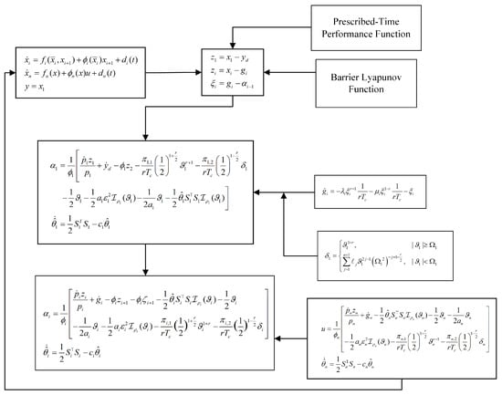
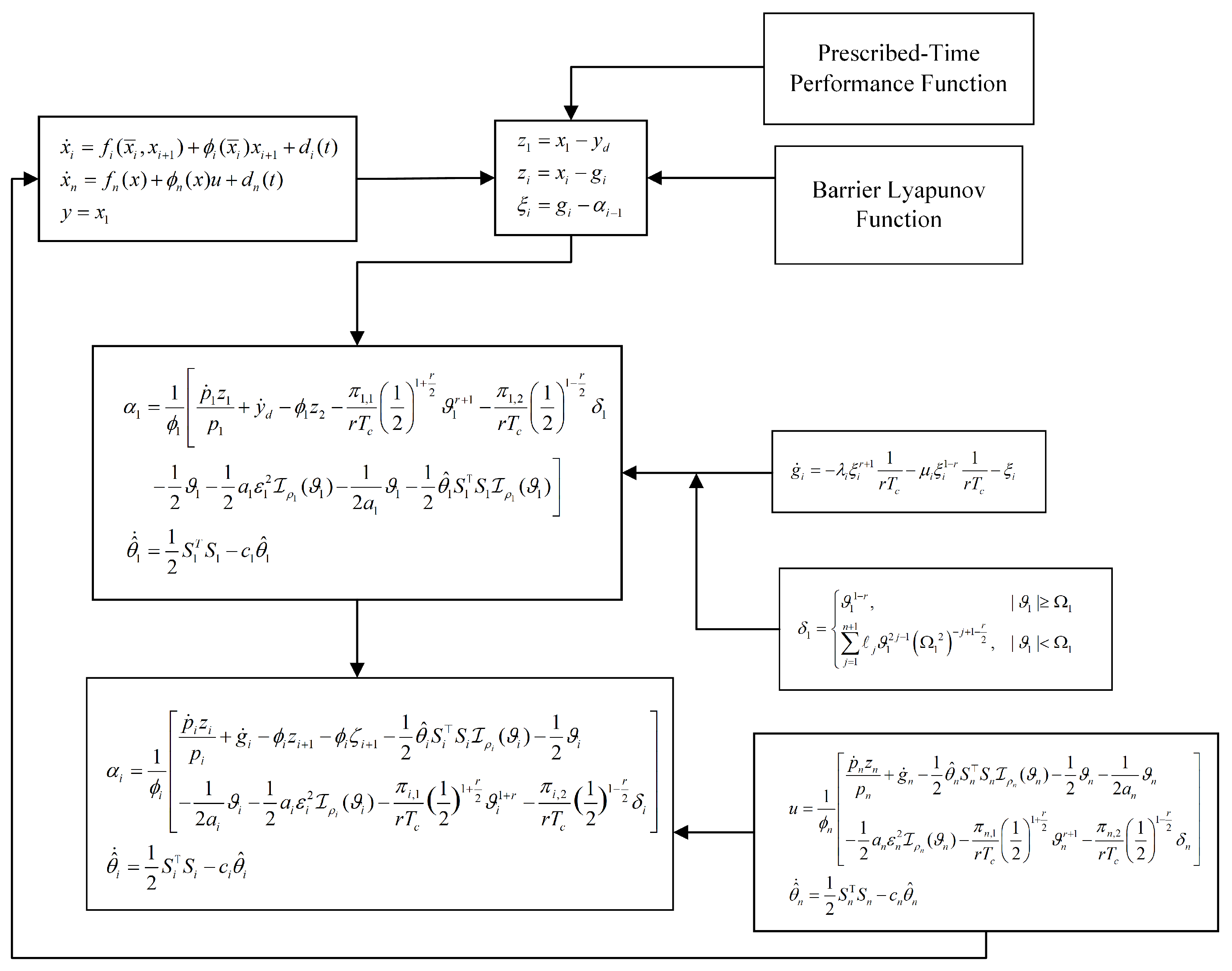
Figure 2 illustrates the overall block diagram of the proposed predefined-time adaptive neural control scheme. It presents the complete recursive design procedure, from error definitions, barrier Lyapunov function, and predefined-time filter to the final virtual and actual control laws.

Figure 2. The block diagram of the control scheme.

4. Simulation

4.1. Simulation Verification on the Brusselator Oscillator

To validate the effectiveness of the proposed predefined-time adaptive neural control scheme, the classic Brusselator oscillator model [35] is employed as the simulation plant.

$$\left\{\begin{array}{c}{\dot{x}}_1=M-(N+1)x_1+x_1^2{x}_2+{\displaystyle \frac{1}{3}}{x}_2^3+x_2+{\overline{d}}_1\left(t\right)\hfill \\ {\dot{x}}_2=N{x}_1-x_1^2{x}_2+\left(2+cos{x}_1\right)u+{\overline{d}}_2\left(t\right)\hfill \\ y=x_1\hfill \end{array}\right.$$

(123)

In this model, the state variables $x_1$ and $x_2$ denote the concentrations of the reaction intermediates and are required to strictly satisfy the practical constraints $|x_1|<3$ and $|x_2|<4$. The external disturbances are selected as ${\overline{d}}_1\left(t\right)=1.2sint$ and ${\overline{d}}_2\left(t\right)=1.2cos\left(1.5t\right)$, and the system constants are set to $M=1$ and $N=3$. The initial conditions are chosen as ${[x_1\left(0\right),x_2\left(0\right)]}^{\mathrm{T}}={[0.1,-0.1]}^{\mathrm{T}}$, and the desired reference trajectory is given by $y_d=0.5sin\left(0.5t\right)$. The design parameters of the controller are tuned according to the proposed scheme as $c_1=1.2$, $c_2=0.25$, and the adaptive gains as $a_1=1.2$, $a_2=0.25$. The parameters of the predefined-time performance function (PTPF) are calibrated to realize the predefined convergence time and set as $p_{1,0}=10$, $p_{1,f}=0.5$, ${\sigma }_1=0.4$, and $p_{2,0}=10$, $p_{2,f}=0.5$, ${\sigma }_2=0.4$, ${\phi }_1={\phi }_2=4.1865$, and the filter parameter is set as $\gamma =0.08$. The numbers of RBF neural network nodes are both set to 11, with centers evenly spaced at $[-0.1,0.1]$ and $[-0.3,0.3]$. The parameters not explicitly listed above are set according to [35].

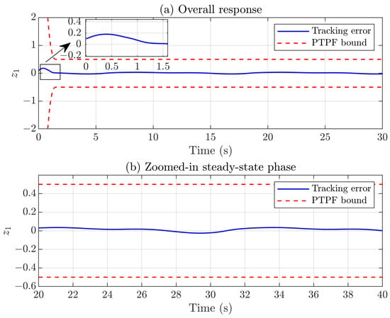
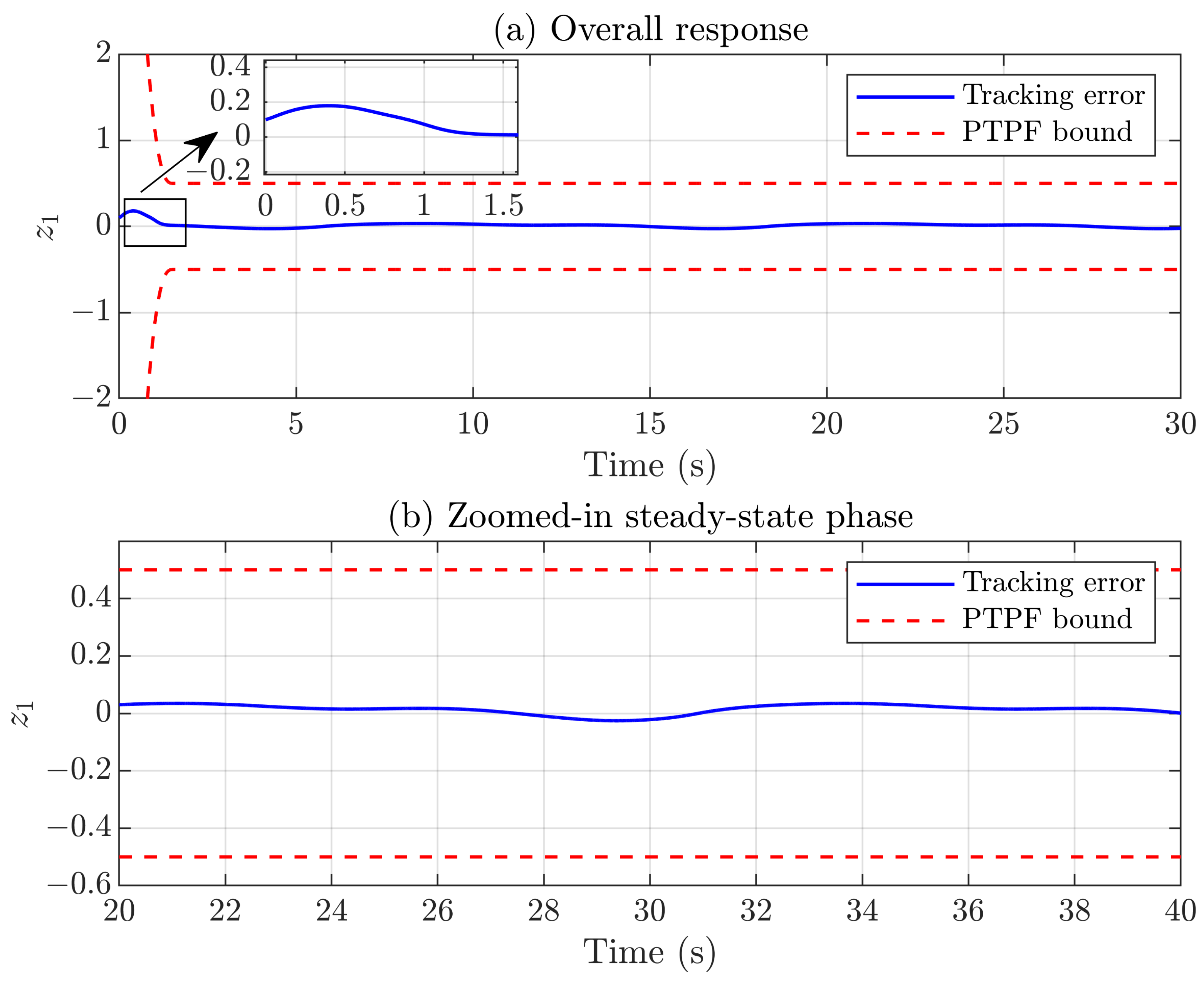
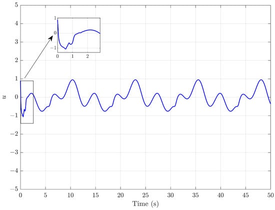
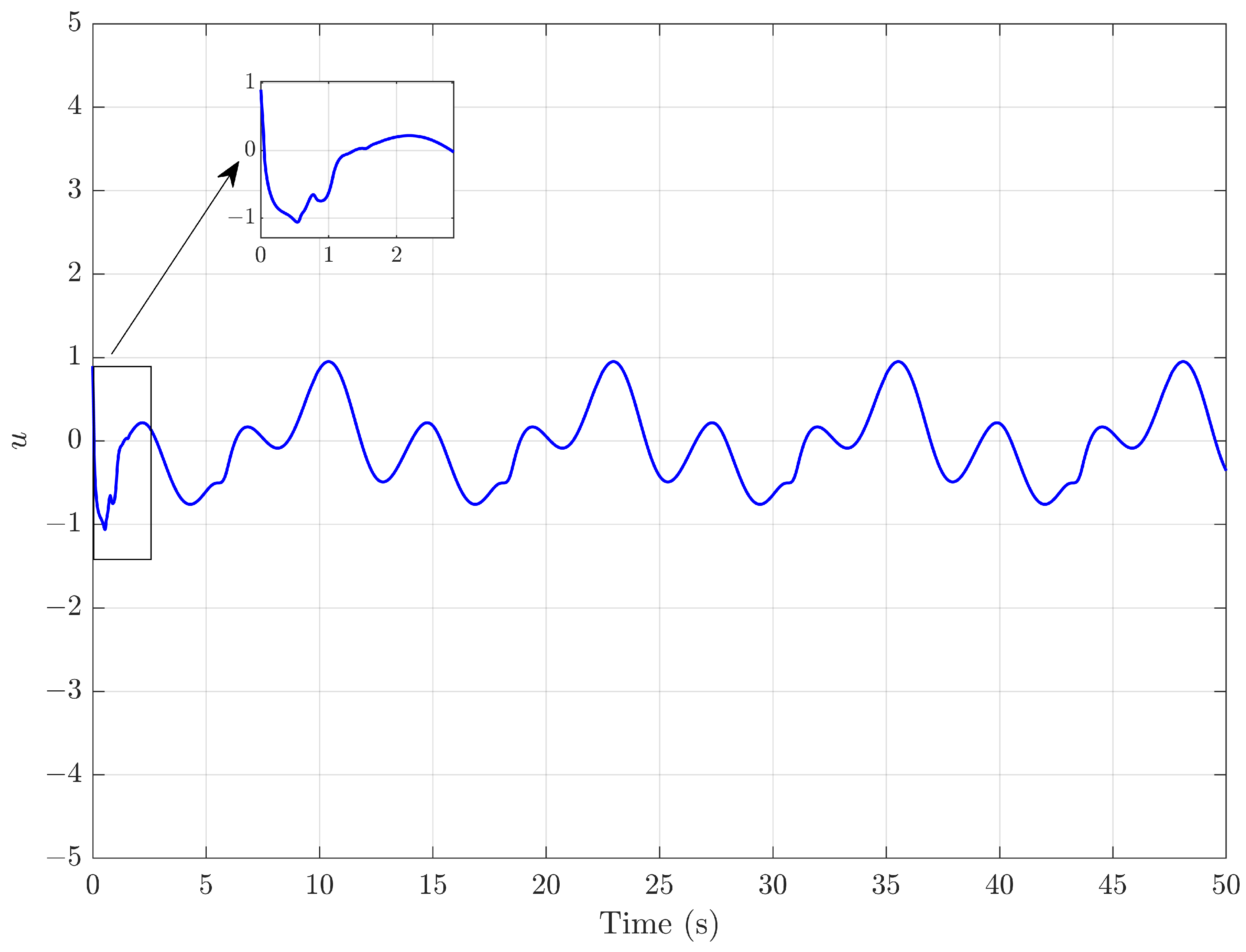
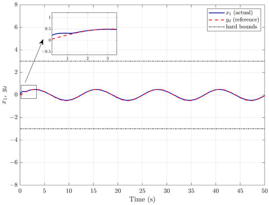
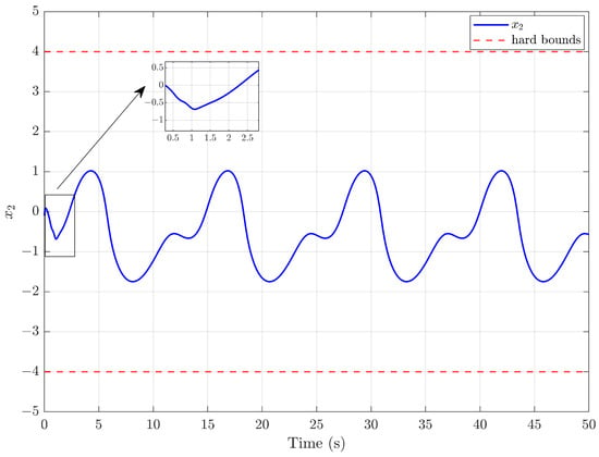
The overall simulation results are demonstrated in Figure 3, Figure 4, Figure 5 and Figure 6. Specifically, Figure 3 depicts the dynamic evolution of tracking error $z_1$, together with predefined-time performance function (PTPF) boundaries, which verifies that the tracking error converges rapidly into the preset steady-state tolerance range within the predefined settling time $T_c=1.5\mathrm{s}$. Figure 4 presents the time-domain variation curve of control input u. Figure 5 and Figure 6 respectively illustrate the trajectory evolution of system state $x_1$ and state $x_2$. It can clearly be observed that both system states are strictly bounded within their respective preset constraint intervals during the whole simulation process, which fully proves the validity of the state-constrained predefined-time tracking control strategy proposed in this work.

Figure 3. Tracking error and PTPF curve.

Figure 4. Control input response.

Figure 5. Response curves of system states $x_1$.

Figure 6. Response curves of system states $x_2$.

Figure 3 shows the tracking error $z_1$ under the proposed scheme. Subfigure (a) displays the overall response, where the tracking error evolves strictly within the PTPF bounds during the entire process. Subfigure (b) zooms into the steady-state phase, clearly demonstrating that the error remains well inside the steady-state bound $\pm p_{1,f}$. These results confirm that the controller fulfills both transient prescribed performance and steady-state accuracy within the predefined time. As shown in Figure 4, the control input exhibits a transient pulse at the initial stage, which quickly eliminates the initial oscillation error. After this brief transient, the control input converges to near zero and remains with negligible fluctuations throughout the remaining simulation period. No sustained oscillation or unbounded surge is observed during the entire process. Such bounded behavior meets the physical constraints of practical actuators, thereby validating the feasibility and reliability of the proposed control law in real engineering applications.

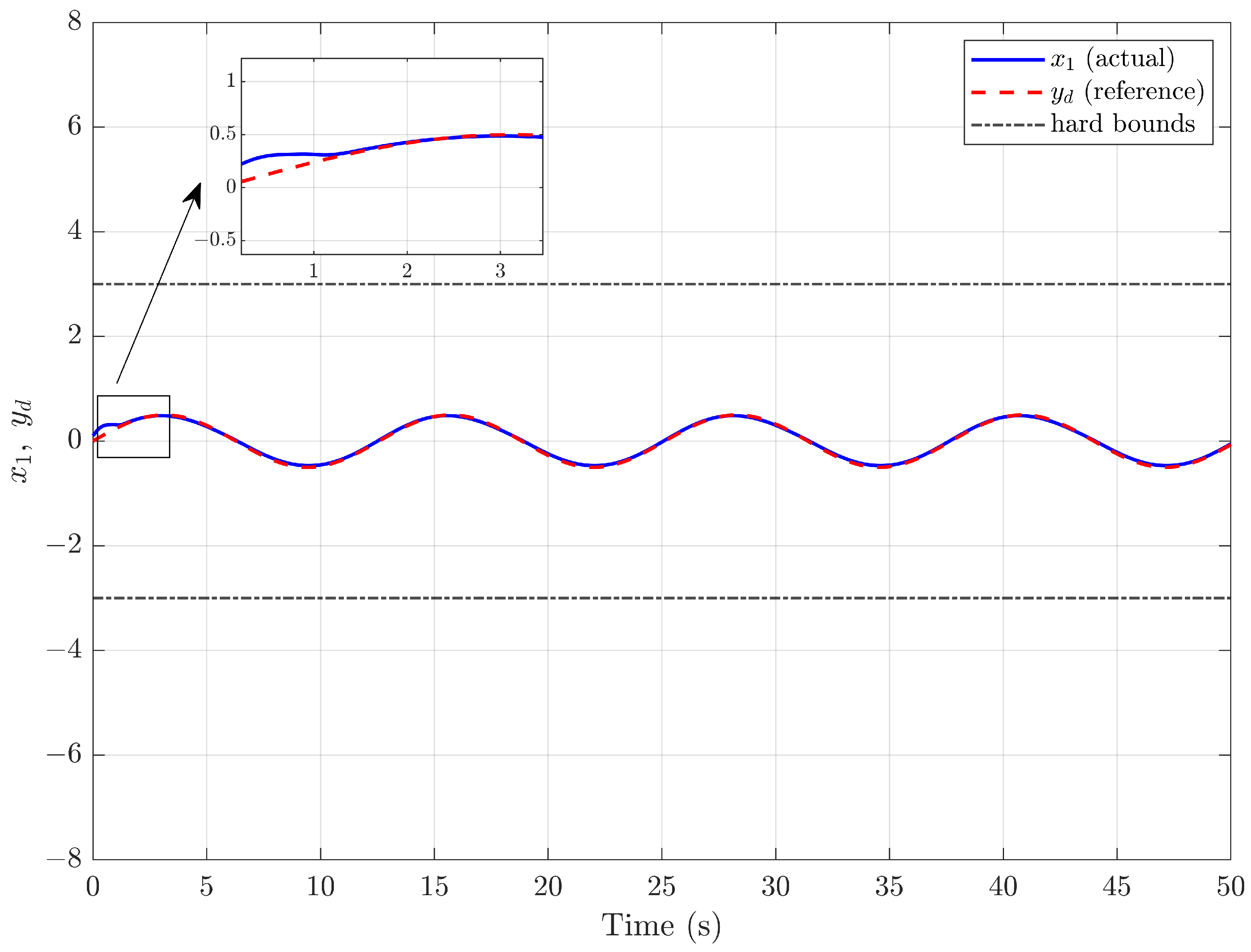
As illustrated in Figure 5, the time response of the system state is presented within 0–$50\mathrm{s}$. The solid blue line represents the actual state $x_1$, the red dashed line denotes the periodic sinusoidal reference trajectory $y_d$, and black dotted lines stand for the hard state constraints. The inset magnifies the initial transient response for clear observation. After a brief transient adjustment, the actual state rapidly tracks the variation tendency of the reference signal. In the steady state, the two curves nearly overlap, with minimal lag, overshoot and steady-state error. This result verifies that the closed-loop system can realize high-precision trajectory tracking for periodic reference commands while complying with full-state constraints.

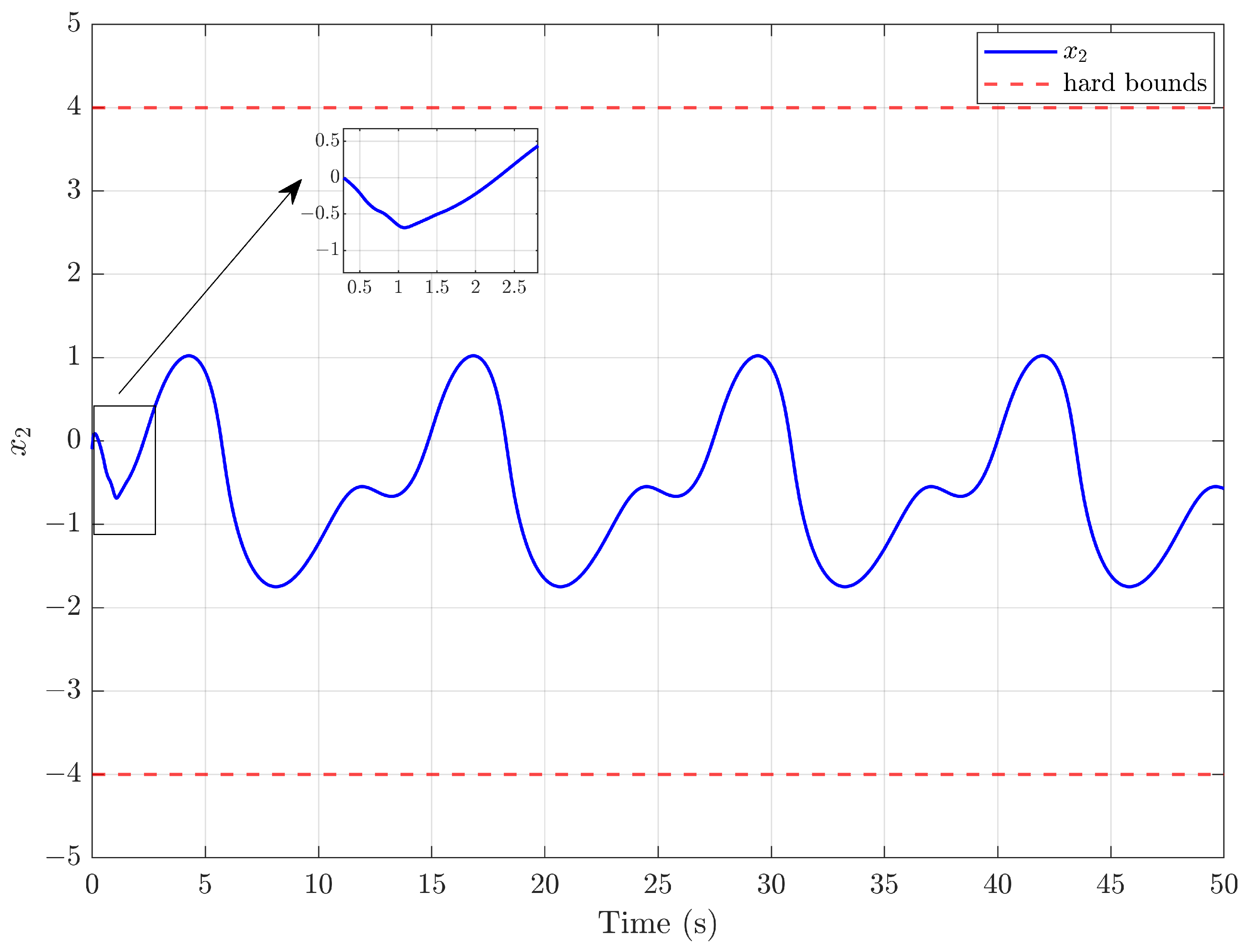
Figure 6 depicts the trajectory evolution of state $x_2$ within 0–50 s. The blue solid curve represents the real-time value of state $x_2$, and two red dashed horizontal lines denote the predefined hard bounds of $+4$ and $-4$. The inset magnifies the initial transient response for clear observation. The state gradually evolves into stable periodic oscillation regulated by the proposed controller. Throughout the whole simulation, $x_2$ never touches or exceeds the preset constraint thresholds, which proves that the designed control scheme can strictly satisfy full-time state constraints and eliminate constraint violation risks.

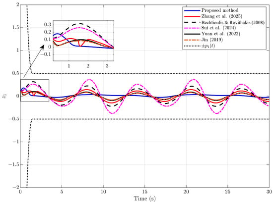
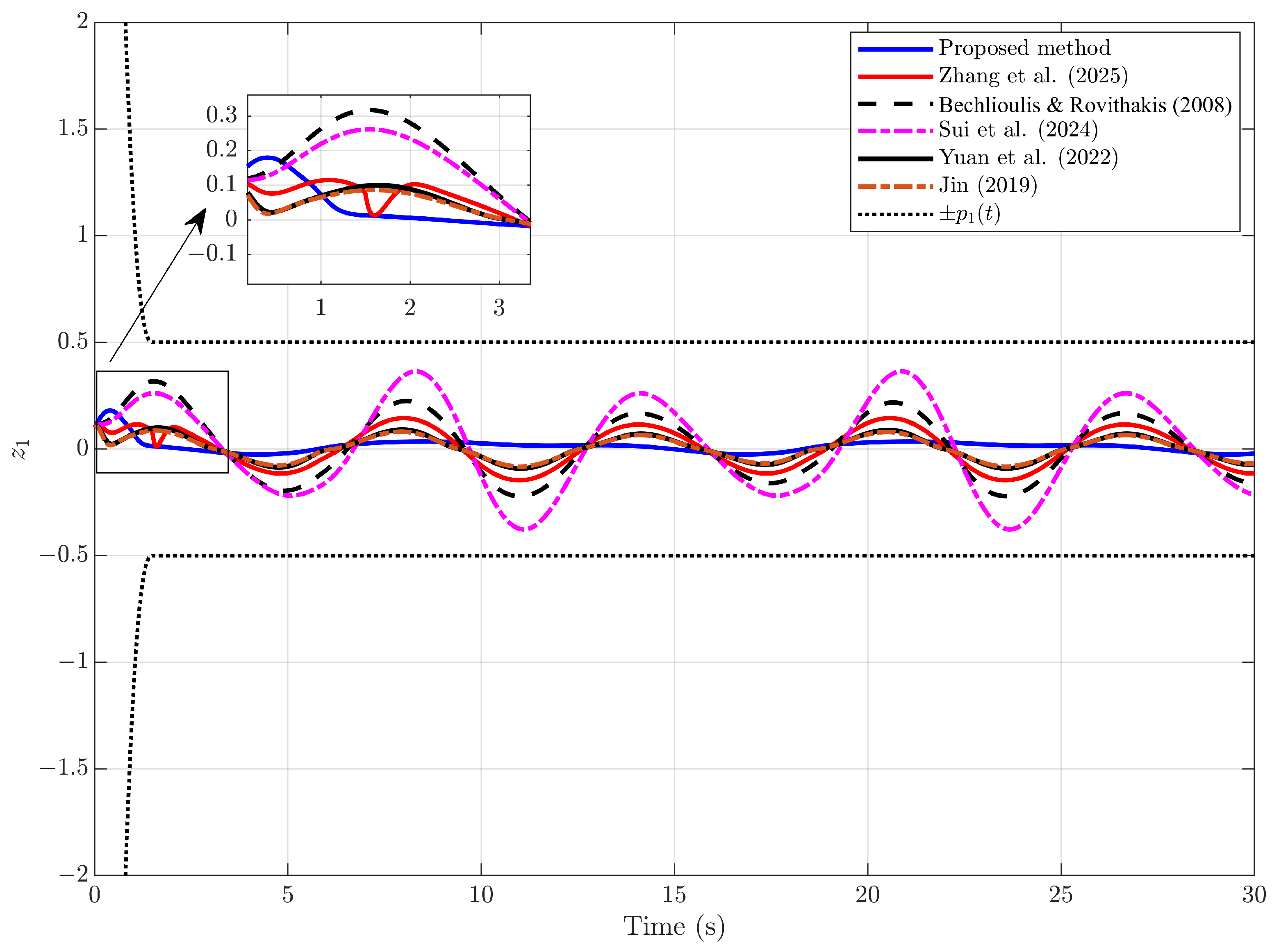
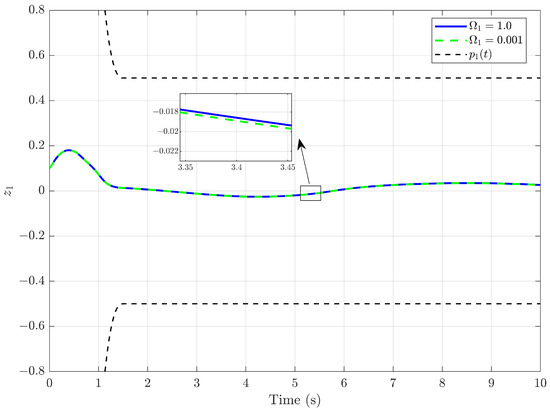
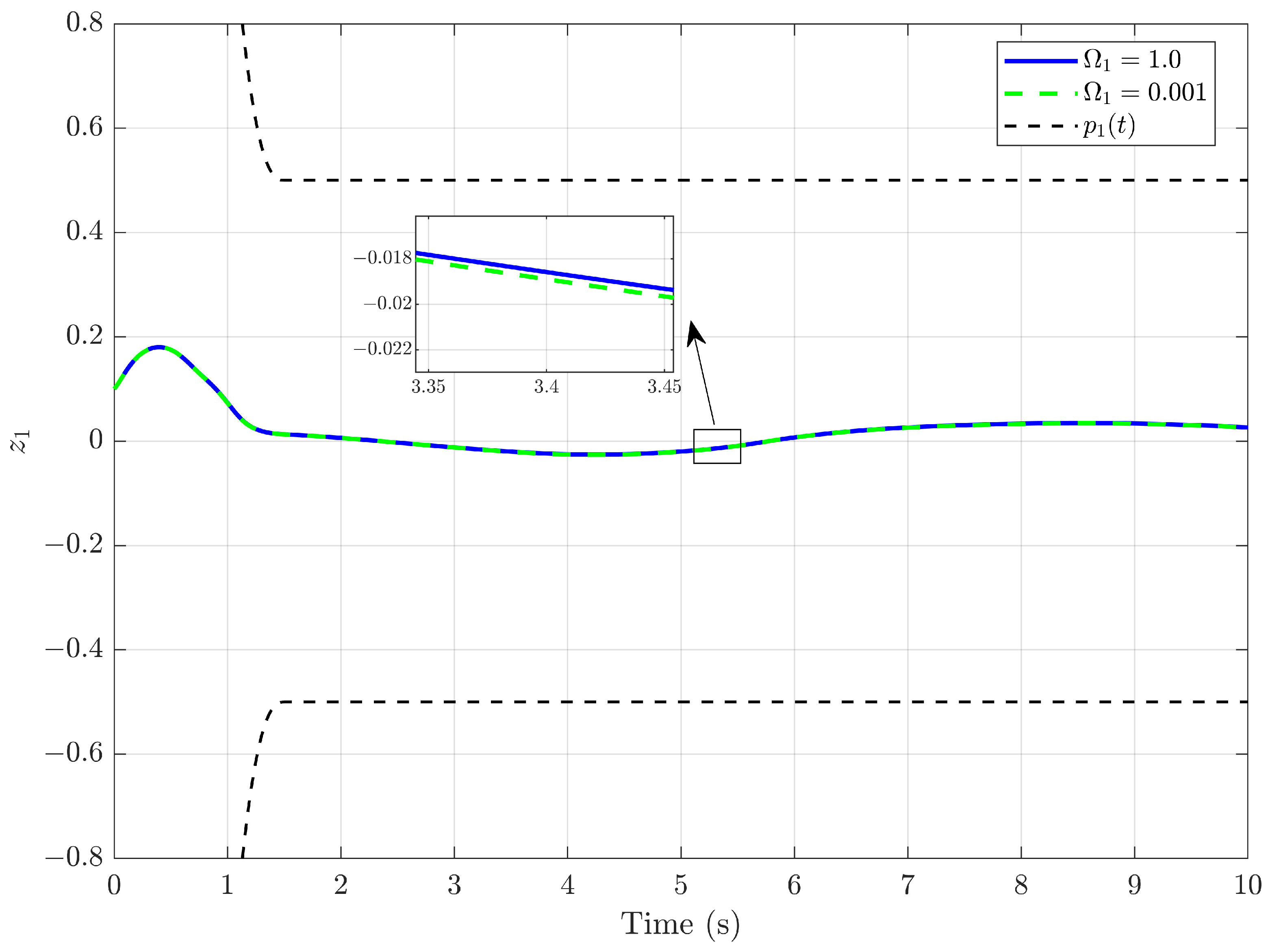
Figure 7 compares the tracking errors of the proposed scheme, the method in [55], the traditional PPC approach [56], the conventional adaptive backstepping method [8], and the finite-time BLF [47] and fixed-time BLF [26] methods. The proposed method achieves the fastest convergence within the prescribed time, the smallest overshoot, and the smoothest steady-state response. In contrast, the conventional backstepping method exhibits the largest overshoot and slowest convergence due to the absence of prescribed performance constraints, while the finite-time and fixed-time BLF methods yield moderate performance. Specifically, although both finite-time and fixed-time BLF methods guarantee finite-time convergence, the convergence time bound of fixed-time BLF is independent of initial errors, whereas that of finite-time BLF depends on them, which may lead to performance variations under different initial conditions. These results clearly demonstrate the superiority of the proposed predefined-time control scheme with PTPF. Figure 8 depicts the tracking error ${\vartheta }_1\left(t\right)$ for different values of ${\Omega }_1$, where ${\Omega }_2$ is kept fixed at $1.0$. Simulation results show that reducing ${\Omega }_1$ contributes to a lower steady-state tracking error. Nevertheless, an excessively small ${\Omega }_1$ is prone to triggering high-frequency oscillations, which demonstrates the inherent trade-off for parameter selection stated in Remark 5. For all comparison methods, the controllers are implemented according to their respective design principles. The parameters of each baseline are carefully tuned to ensure a fair comparison under identical initial conditions and disturbance settings.

Figure 7. Comparison with other existing control methods [8,26,47,55,56].

Figure 8. Comparison Effect of different ${\Omega }_1$ values on tracking performance.

Remark 6.

To ensure impartiality and reproducibility, all comparative simulations among the six schemes evaluated in Figure 7 and Table 3 are conducted under strictly identical plant conditions. Specifically, all methods share the same initial states $x_1\left(0\right)=0.1$, $x_2\left(0\right)=-0.1$, identical external disturbances $d_1\left(t\right)=1.2sint$, $d_2\left(t\right)=1.2cos\left(1.5t\right)$, the same hard constraint bounds $|x_1|<3$, $|x_2|<4$, and the same reference trajectory $y_d=0.5sin\left(0.5t\right)$. The partial experimental data collected under these identical conditions are presented in Table 4. For the method in [55], which was originally designed for strict-feedback systems, we extend it to the pure-feedback model via the mean value theorem in a consistent manner, and tune its parameters strictly according to the original guidelines. The other compared methods (including the conventional PPC [56] and three additional representative controllers from the recent literature) are implemented with their original settings and, where necessary, adapted fairly to the pure-feedback structure without any biased tuning. Therefore, the performance gaps observed in Figure 7 and Table 3 genuinely reflect the inherent advantages of the proposed framework rather than any unfair parameter adjustment.

Table 3. Calculated performance indices.

Index	ISE	ITSE	IAE	IATE
Proposed scheme	0.0453	0.6229	1.1205	25.3838
Zhang, 2025 [55]	0.4312	11.1398	4.1559	105.6633
Finite-time BLF [47]	0.1525	3.6992	2.3630	58.2650
Fixed-time BLF [26]	0.1304	3.1820	2.2109	54.6788
Traditional PPC [56]	1.0808	24.8869	6.5255	157.7004
Traditional Backstepping [8]	2.3685	62.5061	9.5832	246.2958

Table 4. Experimental data (partial).

Time (s)	${\mathbf{x}}_1$	${\mathbf{y}}_{\mathbf{d}}$
6.0	0.078	0.071
6.5	−0.035	−0.054
7.0	−0.149	−0.175
7.5	−0.255	−0.286
8.0	−0.344	−0.378
8.5	−0.413	−0.447
9.0	−0.455	−0.489
9.5	−0.469	−0.500

4.1.1. Robustness Analysis

To further validate the robustness of the proposed control scheme against external disturbances, two groups of disturbances with different amplitudes are tested while keeping all controller parameters unchanged: (i) (baseline): $d_1\left(t\right)=1.2sint$, $d_2\left(t\right)=1.2cos\left(1.5t\right)$ (the same as in the main simulation); (ii) (amplitude doubled): $d_1\left(t\right)=2.4sint$, $d_2\left(t\right)=2.4cos\left(1.5t\right)$. Table 5 summarizes the integral performance indices (ISE, ITSE, IAE, IATE) of the tracking error $z_1$ and the constraint satisfaction status for both disturbance cases. The results show that when the disturbance amplitude is doubled, the ISE index slightly increases from the baseline value of $0.0453$ to $0.0727$. Although all indices increase to some extent, they remain at relatively low levels. Under both cases, the system states strictly satisfy the prescribed constraint bounds $|x_1|<3$, $|x_2|<4$, and the tracking error consistently converges to the predefined residual set without divergence or instability. These results demonstrate that the proposed control scheme possesses favorable robustness against external disturbances with varying amplitudes.

Table 5. Effect of amplitude doubling on the calculated performance indices.

Index	ISE	ITSE	IAE	IATE
Baseline	0.0453	0.6229	1.1205	25.3838
Amplitude doubled	0.0727	0.8102	1.2868	27.1413

In addition to external disturbances, the robustness against internal parameter variations is also evaluated. Table 6 summarizes the results of the parametric sensitivity analysis, where the key design parameters $T_c$ and r are perturbed by $\pm 20\%$ from their nominal values. Specifically, three performance indices are examined: the maximum absolute tracking error $max|z_1|$, the convergence time $t_s$, and the steady-state root-mean-square error (RMSE). It is observed that all three indices remain close to their nominal levels under the tested parameter deviations, and the state constraints are strictly satisfied in all cases. These results confirm that the proposed control scheme exhibits low sensitivity to parameter perturbations and does not require precise parameter tuning for reliable operation in practice.

Table 6. Parameter sensitivity analysis results.

Parameter	Variation	$max|{\mathit{z}}_1|$	${\mathit{t}}_{\mathit{s}}$ (s)	RMSE
$T_c$	1.2 s	0.2384	1.5000	0.0245
	1.5 s	0.2466	1.5000	0.0251
	1.8 s	0.2546	1.5000	0.0256
r	0.32	0.2414	1.5000	0.0238
	0.4	0.2466	1.5000	0.0251
	0.48	0.2507	1.5000	0.0261

4.1.2. Computational Complexity and Real-Time Feasibility

To assess the engineering applicability of the proposed control algorithm, this subsection analyzes its computational cost. Compared with the conventional backstepping method, the additional computational overhead mainly arises from three sources: (i) the predefined-time dynamic surface filter, (ii) the online adaptive update of the RBF neural networks, and (iii) the piecewise smooth function ${\delta }_i$ introduced to eliminate controller singularities. In the simulation environment, the total elapsed time for a 50 s simulation is 2.92 s, corresponding to an average of 0.117 ms per time step. Even with the filter dynamics and RBF updates included simultaneously, the per-step computation remains well below the sub-millisecond level, which is far smaller than the typical sampling period of most physical systems.

From the perspective of algorithmic complexity, the number of RBF nodes is fixed at 11, the piecewise function ${\delta }_i$ involves only elementary algebraic operations, and the filter and adaptive laws are essentially evaluations of right-hand-side functions of ordinary differential equations. Consequently, the overall control law has a computational complexity of $O(n·N_{\mathrm{RBF}})$, where n is the system order and $N_{\mathrm{RBF}}$ is the number of neural network nodes. For the current second-order example, this complexity is of constant order; as the system order increases, it grows only linearly without any exponential explosion. In summary, despite the introduction of the predefined-time mechanism and neural network compensation, the computational burden is well within the affordable range of modern industrial controllers, thereby confirming its real-time deployment feasibility.

4.2. Higher-Order Numerical Example

To further verify the generality of the proposed control scheme for higher-order ($n\ge 3$) pure-feedback systems, this subsection considers a third-order pure-feedback nonlinear system. The system dynamics are given by

$$\left\{\begin{array}{c}{\dot{x}}_1=f_1({\overline{x}}_1,x_2)+{\varphi }_1\left({\overline{x}}_1\right)x_2+d_1\left(t\right)\hfill \\ {\dot{x}}_2=f_2({\overline{x}}_2,x_3)+{\varphi }_2\left({\overline{x}}_2\right)x_3+d_2\left(t\right)\hfill \\ {\dot{x}}_3=f_3\left(x\right)+{\varphi }_3\left(x\right)u+d_3\left(t\right)\hfill \\ y=x_1\hfill \end{array}\right.$$

(124)

where the nonlinear functions are chosen as $f_1=x_1{e}^{-0.5x_1}+0.2x_2^3,$ ${\varphi }_1=1+0.5sin\left(x_1\right),$ $f_2=x_{1}sin\left(x_2\right)+0.3x_3^2,$ ${\varphi }_2=2+cos\left(x_1{x}_2\right),$ $f_3=0.5x_1{x}_2+0.2cos\left(x_3\right),$ ${\varphi }_3=3+sin\left(x_1{x}_2{x}_3\right).$ The state constraints are set as $|x_1|<1.5$, $|x_2|<2$, $|x_3|<2.5$. The reference signal is given by $y_d=0.5sin\left(0.5t\right)$, and the external disturbances are taken as $d_i\left(t\right)=0.2sin\left(t\right)(i=1,2,3)$.

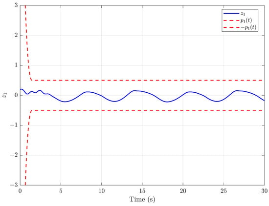
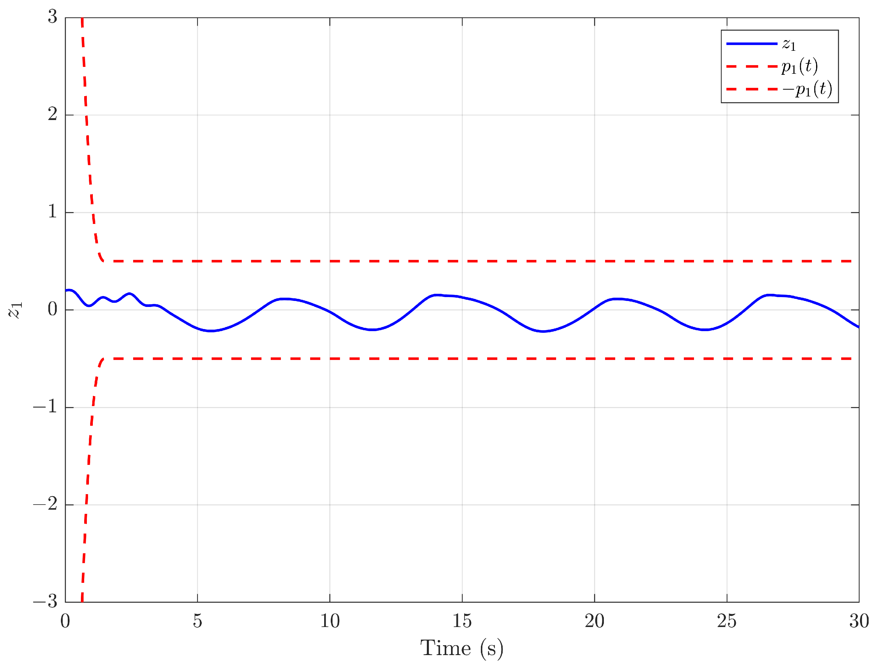
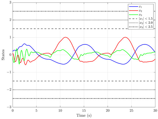
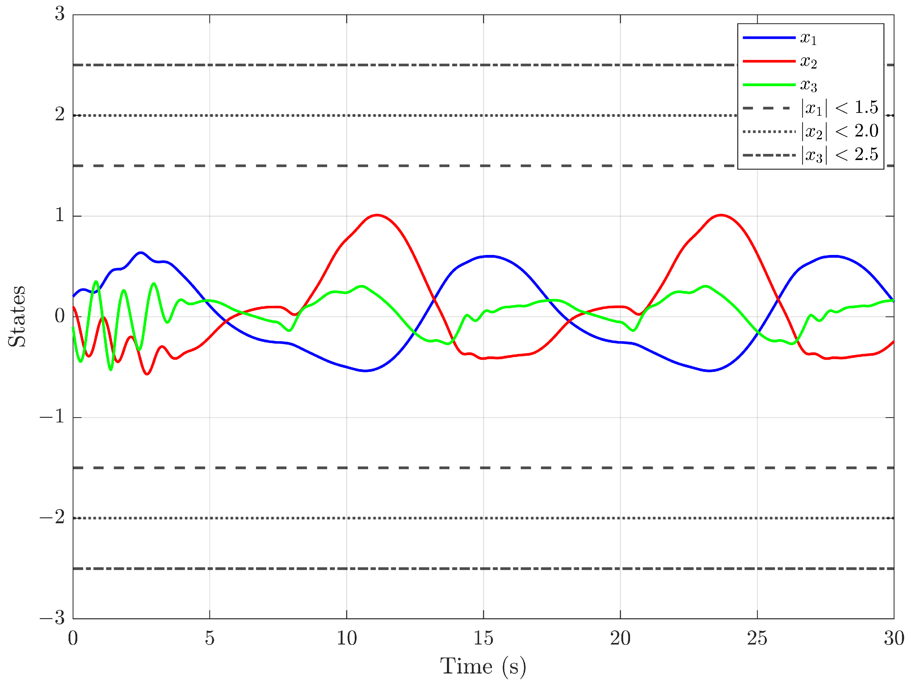
In the simulation, the parameters of the predefined-time performance functions (PTPFs) are uniformly set to $p_{1,0}=p_{2,0}=p_{3,0}=10$, $p_{1,f}=p_{2,f}=p_{3,f}=0.5$, ${\sigma }_1={\sigma }_2={\sigma }_3=0.4$, and ${\varphi }_1={\varphi }_2={\varphi }_3=4.1865$, leading to the prescribed settling times $T_{1,p}\approx T_{2,p}\approx T_{3,p}\approx 1.5$ s. The controller parameters are selected as $T_c=1.5$, $r=0.4$, and the filter time constants are ${\gamma }_2={\gamma }_3=0.5$. The design gains are configured as ${\pi }_{11}={\pi }_{21}={\pi }_{31}=0.4$ and ${\pi }_{12}={\pi }_{22}={\pi }_{32}=0.15$. The initial conditions are $x_1\left(0\right)=0.2$, $x_2\left(0\right)=0.1$, $x_3\left(0\right)=-0.1$, with all initial filter states set to zero. It should be noted that, in this particular higher-order verification, the system nonlinearities $f_1$, $f_2$, and $f_3$ are assumed to be known purely to examine the algebraic scalability and constraint-enforcement capability of the proposed recursive framework. This simplification does not compromise the generality, since the neural-network approximation modules can be directly incorporated to handle fully unknown dynamics without altering the control structure. The simulation results shown in Figure 9 and Figure 10 depict the evolution of the tracking error $z_1=x_1-y_d$, along with its predefined-time performance bounds $\pm p_1\left(t\right)$. It is observed that $z_1$ remains strictly within the prescribed bounds during the convergence phase ($t<T_{1,p}$) and enters the steady-state region smoothly after about 1.5 s, which verifies the predefined-time constraint satisfaction. Figure 10 presents the response trajectories of states $x_1$, $x_2$, and $x_3$, together with their respective hard constraint boundaries (dashed, dotted, and dash-dotted lines denote $|x_1|<1.5$, $|x_2|<2.0$, and $|x_3|<2.5$, respectively). All state variables are maintained strictly within their predefined limits over the entire simulation horizon, exhibiting smooth transients without overshoot. These results clearly demonstrate that the proposed control law can be effectively generalized to third-order systems, ensuring both predefined-time convergence and rigorous satisfaction of multiple hard state constraints, thereby confirming its universality for higher-order, pure-feedback, nonlinear systems.

Figure 9. Tracking error and PTPF bound.

Figure 10. State trajectories with hard constraints.

5. Conclusions

This paper has developed a predefined-time adaptive neural tracking control scheme for a class of nonlinear pure-feedback systems subject to full-state constraints. The core innovation lies in the construction of a novel barrier Lyapunov function that seamlessly integrates a predefined-time performance function, which not only strictly enforces the prescribed bounds on all system states throughout the entire operation but also ensures that the tracking error converges to a prespecified residual set within an arbitrarily user-assigned settling time, independent of initial conditions and design parameters. To circumvent the “complexity explosion” issue inherent in conventional backstepping, a predefined-time dynamic surface filter is introduced, whose stability and convergence time are rigorously proven. Meanwhile, radial basis function neural networks are employed to approximate the unknown system nonlinearities online, with adaptive laws updating the weight estimates in real time, thereby eliminating the requirement for precise mathematical models. Rigorous Lyapunov-based stability analysis has established that all signals in the closed-loop system are predefined-time-bounded. Comprehensive simulations on the benchmark Brusselator oscillator model, under time-varying external disturbances and strict physical concentration constraints, substantiate the theoretical findings. The results vividly demonstrate that: (i) the tracking error rapidly enters and remains within the prescribed steady-state boundary before the predefined time elapses; (ii) both system states strictly adhere to their respective constraint limits without any violation; (iii) the control input remains smooth, bounded, and practically feasible; and (iv) quantitative comparisons with existing schemes reveal significantly lower ISE, ITSE, IAE, and IATE indices, confirming superior transient performance and cumulative error suppression. Overall, the proposed strategy offers a robust, high-precision, and constraint-guaranteed solution for complex nonlinear systems with hard state restrictions. Future research will focus on several concrete open problems arising from the present framework. In particular, it would be meaningful to relax Assumption 1 by allowing the effective control gain ${\displaystyle \frac{\partial f_i}{\partial x_{i+1}}}+{\varphi }_i$ to vanish or change sign at isolated points, which would require singularity-free adaptive designs and may substantially extend the applicability of the proposed method. Another direction is to consider output-feedback scenarios where only the output $x_1$ is measurable and the control directions may be unknown, since the current scheme relies on full-state feedback and known control directions. Additionally, the simultaneous presence of actuator faults and unknown input quantization under the predefined-time performance requirement remains an open and practically relevant problem, as it combines multiplicative actuator uncertainties with discontinuous input characteristics.

It is worth noting that the proposed predefined-time neural control scheme is developed for ODE-based nonlinear systems. However, many practical engineering systems, such as thermal processes, fluid dynamics, and chemical reactions, are inherently spatiotemporal in nature and are more accurately modeled by partial differential equations (PDEs). Extending the proposed predefined-time control framework to such distributed parameter systems presents several nontrivial challenges, including the approximation of spatiotemporal uncertainties and the design of boundary or distributed controllers that guarantee predefined-time convergence in infinite-dimensional spaces. Recent advances in neural-network-based approximation for spatiotemporal systems, such as the congealed neural network (Con NN) approach, provide a promising avenue for addressing the uncertainty approximation issue in PDE systems. The ConNN structure, which decomposes time-varying uncertainties into congealed weights and time-dependent perturbations, aligns well with the adaptive estimation framework required for predefined-time control design. Integrating such spatiotemporal approximation techniques with predefined-time stability theory—for instance, via PDE backstepping or operator-based methods—constitutes an important direction for our future work.

References

- Yang, G.C.; Yao, J.Y. Multilayer neurocontrol of high-order uncertain nonlinear systems with active disturbance rejection. Int. J. Robust Nonlinear Control 2024, 34, 2972–2987. [Google Scholar] [CrossRef] [Scilit]
- Chen, G.J.; Dong, J.X. Approximate Optimal Adaptive Prescribed Performance Control for Uncertain Nonlinear Systems with Feature Information. IEEE Trans. Syst. Man Cybern. Syst. 2024, 54, 2298–2308. [Google Scholar] [CrossRef] [Scilit]
- Arena, P.; Fortuna, L.; Frasca, M.; Sicurella, G. An Adaptive, Self-Organizing Dynamical System for Hierarchical Control of Bio-Inspired Locomotion. IEEE Trans. Syst. Man Cybern. Part B Cybern. 2004, 34, 1823–1837. [Google Scholar] [CrossRef] [Scilit] [PubMed]
- Wang, Y.Z.; Duan, G.R.; Li, P. Event-Triggered Adaptive Sliding Mode Control of Uncertain Nonlinear Systems Based on Fully Actuated System Approach. IEEE Trans. Circuits Syst. II Express Briefs 2024, 71, 2749–2753. [Google Scholar] [CrossRef] [Scilit]
- Liu, J.C.; Liu, J.; Yan, R.D.; Ding, T. Deep Lyapunov Learning: Embedding the Lyapunov Stability Theory in Interpretable Neural Networks for Transient Stability Assessment. IEEE Trans. Power Syst. 2024, 39, 7437–7440. [Google Scholar] [CrossRef] [Scilit]
- Ambe, H.; Nguimfack-Ndongmo, J.D.D.; Alombah, N.H.; Aloyem, C.V.; Kazé; Kuate-Fochie, R.; Asoh, D.A.; Nfah, E.M. Robust nonlinear MPPT controller for PV energy systems using PSO-based integral backstepping and artificial neural network techniques. Int. J. Dyn. Control 2024, 12, 1598–1615. [Google Scholar] [CrossRef] [Scilit]
- Eneyew, G.M.; Asfaw, W.A.; Abdissa, C.M. Optimized Backstepping Fuzzy Sliding Mode Controller for Trajectory Tracking of Mobile Manipulator. Eng. Rep. 2025, 7, e70269. [Google Scholar] [CrossRef] [Scilit]
- Sui, S.; Chen, C.L.P.; Tong, S.C. Command Filter-Based Predefined Time Adaptive Control for Nonlinear Systems. IEEE Trans. Autom. Control 2024, 69, 7863–7870. [Google Scholar] [CrossRef] [Scilit]
- Liu, S.; Ge, S.; Zhang, J. Adaptive output-feedback control for a class of uncertain stochastic non-linear systems with time delays. Int. J. Control 2008, 81, 1210–1220. [Google Scholar] [CrossRef] [Scilit]
- Min, H.; Xu, S.; Zhang, B.; Ma, Q. Output-feedback control for stochastic nonlinear systems subject to input saturation and timevarying delay. IEEE Trans. Autom. Control 2019, 64, 359–364. [Google Scholar] [CrossRef] [Scilit]
- Chen, W.S.; Wu, J.; Jiao, L.C. State-feedback stabilization for a class of stochastic time-delay nonlinear systems. Int. J. Robust Nonlinear Control 2012, 22, 1921–1937. [Google Scholar] [CrossRef] [Scilit]
- Liu, T.; Chen, Y.Y.; Li, S. Adaptive Cooperative Estimation and Guidance Against Unknown Maneuvering Target. IEEE Trans. Aerosp. Electron. Syst. 2025, 61, 9129–9140. [Google Scholar] [CrossRef] [Scilit]
- Zou, W.; Ahn, C.K.; Xiang, Z. Analysis on existence of compact set in neural network control for nonlinear systems. Automatica 2020, 120, 109155. [Google Scholar] [CrossRef] [Scilit]
- Min, H.; Shi, S.; Xu, S.; Guo, J.; Zhang, Z. Fixed-time Lyapunov criteria of stochastic nonlinear systems and its generalization. IEEE Trans. Autom. Control 2023, 68, 5052–5058. [Google Scholar] [CrossRef] [Scilit]
- Song, S.; Zhang, B.; Xia, J.; Zhang, Z. Adaptive backstepping hybrid fuzzy sliding mode control for uncertain fractional-order nonlinear systems based on finite-time scheme. IEEE Trans. Syst. Man Cybern. Syst. 2020, 50, 1559–1569. [Google Scholar] [CrossRef] [Scilit]
- Zhao, X.; Wang, X.; Zhang, S.; Zong, G. Adaptive neural backstepping control design for a class of nonsmooth nonlinear systems. IEEE Trans. Syst. Man Cybern. Syst. 2019, 49, 1820–1831. [Google Scholar] [CrossRef] [Scilit]
- Sui, S.; Chen, C.L.P.; Tong, S. Neural network filtering control design for nontriangular structure switched nonlinear systems in finite time. IEEE Trans. Neural Netw. Learn. Syst. 2019, 30, 2153–2162. [Google Scholar] [CrossRef] [Scilit] [PubMed]
- Liu, Z.; Chen, B.; Lin, C. Adaptive neural backstepping for a class of switched nonlinear system without strict-feedback form. IEEE Trans. Syst. Man Cybern. Syst. 2017, 47, 1315–1320. [Google Scholar] [CrossRef] [Scilit]
- Wang, Q.; Cao, J.; Liu, H. Adaptive Fuzzy Control of Nonlinear Systems with Predefined Time and Accuracy. IEEE Trans. Fuzzy Syst. 2022, 30, 5152–5165. [Google Scholar] [CrossRef] [Scilit]
- Murari, A.; Vagliasindi, G.; Arena, P.; Fortuna, L.; Barana, O.; Johnson, M.; JET-EFDA Contributors. Prototype of an Adaptive Disruption Predictor for JET Based on Fuzzy Logic and Regression Trees. Nucl. Fusion 2008, 48, 035010. [Google Scholar] [CrossRef] [Scilit]
- Lv, Z.Y.; Zhao, Q.; Sun, X.M.; Wu, Y.H. Finite-Time Control Design for a Coaxial Tilt-Rotor UAV. IEEE Trans. Ind. Electron. 2024, 71, 16132–16142. [Google Scholar] [CrossRef] [Scilit]
- Bhat, S.P.; Bernstein, D.S. Finite-time stability of continuous autonomous systems. SIAM J. Control Optim. 2000, 38, 751–766. [Google Scholar] [CrossRef] [Scilit]
- Qiu, J.; Wang, T.; Sun, K.; Rudas, I.J.; Gao, H. Disturbance observerbased adaptive fuzzy control for strict-feedback nonlinear systems with finite-time prescribed performance. IEEE Trans. Fuzzy Syst. 2022, 30, 1175–1184. [Google Scholar] [CrossRef] [Scilit]
- Yan, Z.; Pan, Z.; Hu, G.; Cheng, J.; Qi, W. Annular Finite-Time H2/H∞ Control for Mean-Field Jump-Diffusion Systems. IEEE Trans. Cybern. 2025, 55, 5358–5371. [Google Scholar] [CrossRef] [Scilit] [PubMed]
- Polyakov, A. Nonlinear feedback design for fixed-time stabilization of linear control systems. IEEE Trans. Autom. Control 2012, 57, 2106–2110. [Google Scholar] [CrossRef] [Scilit]
- Jin, X. Adaptive fixed-time control for MIMO nonlinear systems with asymmetric output constraints using universal barrier functions. IEEE Trans. Autom. Control 2019, 64, 3046–3053. [Google Scholar] [CrossRef] [Scilit]
- Sánchez-Torres, J.D.; Gómez-Gutiérrez, D.; López, E.; Loukianov, A.G. A class of predefined-time stable dynamical systems. IMA J. Math. Control Inf. 2018, 35, i1–i29. [Google Scholar] [CrossRef] [Scilit]
- Jiménez-Rodríguez, E.; Muñoz Vázquez, A.J.; Sánchez-Torres, J.D.; Loukianov, A.G. A note on predefined-time stability. IFAC-PapersOnLine 2018, 51, 520–525. [Google Scholar] [CrossRef] [Scilit]
- Sánchez-Torres, J.D.; Muñoz Vázquez, A.J.; Defoort, M.; Jiménez-Rodríguez, E.; Loukianov, A.G. A class of predefined-time controllers for uncertain second-order systems. Eur. J. Control 2020, 53, 52–58. [Google Scholar] [CrossRef] [Scilit]
- Ni, J.; Liu, L.; Tang, Y.; Liu, C. Predefined-time consensus tracking of second-order multiagent systems. IEEE Trans. Syst. Man Cybern. Syst. 2021, 51, 2550–2560. [Google Scholar] [CrossRef] [Scilit]
- Muñoz Vázquez, A.J.; Sánchez-Torres, J.D.; Gutiérrez-Alcalá, S.; Jiménez-Rodríguez, E.; Loukianov, A.G. Predefined-time robust contour tracking of robotic manipulators. J. Frankl. Inst. 2019, 356, 2709–2722. [Google Scholar] [CrossRef] [Scilit]
- Muñoz Vázquez, A.J.; Sánchez-Torres, J.D.; Jiménez-Rodríguez, E.; Loukianov, A.G. Predefined-time robust stabilization of robotic manipulators. IEEE/ASME Trans. Mechatron. 2019, 24, 1033–1040. [Google Scholar] [CrossRef] [Scilit]
- Guo, S.; Pan, Y.; Li, H.; Cao, L. Dynamic Event-Driven ADP for N-Player Nonzero-Sum Games of Constrained Nonlinear Systems. IEEE Trans. Autom. Sci. Eng. 2024, 22, 7657–7669. [Google Scholar] [CrossRef] [Scilit]
- Pan, Y.N.; Chen, Y.L.; Liang, H.J. Event-triggered predefined-time control for full-state constrained nonlinear systems: A novel command filtering error compensation method. Sci. China Technol. Sci. 2024, 67, 2867–2880. [Google Scholar] [CrossRef] [Scilit]
- Liu, W.; Zhao, J.H.; Zhao, H.Y.; Ma, Q.; Xu, S.Y.; Park, J.H. Neural Preassigned Performance Control for State-Constrained Nonlinear Systems Subject to Disturbances. IEEE Trans. Neural Netw. Learn. Syst. 2025, 36, 5032–5043. [Google Scholar] [CrossRef] [Scilit] [PubMed]
- Zhang, T.; Xia, M.; Yi, Y. Adaptive neural dynamic surface control of strict-feedback nonlinear systems with full state constraints and unmodeled dynamics. Automatica 2017, 81, 232–239. [Google Scholar] [CrossRef] [Scilit]
- Li, D.; Tong, S.; Yang, H.; Hu, Q. Time-Synchronized Control for Spacecraft Reorientation with Time-Varying Constraints. IEEE/ASME Trans. Mechatron. 2025, 30, 2073–2083. [Google Scholar] [CrossRef] [Scilit]
- Liu, K.; Jiao, L.; Zhang, Y.; Zhao, P. Adaptive Predefined-Time Prescribed Performance Control with Application to a Quadrotor UAV. IEEE Trans. Aerosp. Electron. Syst. 2026, 62, 4751–4770. [Google Scholar] [CrossRef] [Scilit]
- Zhu, Z.; Zhu, Q. Adaptive Neural Prescribed Performance Control for Non-Triangular Structural Stochastic Highly Nonlinear Systems Under Hybrid Attacks. IEEE Trans. Autom. Sci. Eng. 2024, 22, 6543–6553. [Google Scholar] [CrossRef] [Scilit]
- Gou, M.; Wang, B.; Zhang, X. Development of Multi-Motor Servo Control System Based on Heterogeneous Embedded Platforms. Electronics 2024, 13, 2957. [Google Scholar] [CrossRef] [Scilit]
- Liu, Y.J.; Chen, H. Adaptive sliding mode control for uncertain active suspension systems with prescribed performance. IEEE Trans. Syst. Man Cybern. Syst. 2021, 51, 6414–6422. [Google Scholar] [CrossRef] [Scilit]
- He, W.; Xu, R. Adaptive Neural Predefined-Time Dynamic Surface Control for Nonlinear Multi-Agent Systems with Input Quantisation via Global Prescribed-Time Performance. Int. J. Control 2026, 99, 2853–2874. [Google Scholar] [CrossRef] [Scilit]
- Xu, Z.; Deng, W.; Shen, H.; Yao, J. Extended-state-observer-based adaptive prescribed performance control for hydraulic systems with fullstate constraints. IEEE/ASME Trans. Mechatron. 2022, 27, 5615–5625. [Google Scholar] [CrossRef] [Scilit]
- Liu, T.; Chen, Y.Y.; Ge, X. Congealed Neural Network Design for Uncertain Nonlinear Spatiotemporal Control Systems. Automatica 2026, 183, 112636. [Google Scholar] [CrossRef] [Scilit]
- Liu, W.; Fei, S.; Ma, Q.; Zhao, H.; Xu, S. Prescribed performance dynamic surface control for nonlinear systems subject to partial and full state constraints. Appl. Math. Comput. 2022, 431, 127318. [Google Scholar] [CrossRef] [Scilit]
- Zhu, G.; Zhang, X.; Li, H.; Zhang, X.; Su, C. Finite Time Prescribed Performance Adaptive Consensus Control for Nonlinear Multi-Agent Systems and Its Application. IEEE Trans. Autom. Sci. Eng. 2025, 22, 22484–22496. [Google Scholar] [CrossRef] [Scilit]
- Yuan, X.; Chen, B.; Lin, C. Prescribed finite-time adaptive neural tracking control for nonlinear state-constrained systems: Barrier function approach. IEEE Trans. Neural Netw. Learn. Syst. 2022, 33, 7513–7522. [Google Scholar] [CrossRef] [Scilit] [PubMed]
- Wang, N.; Fu, Z.; Song, S.; Wang, T. Barrier-Lyapunov-based adaptive fuzzy finite-time tracking of pure-feedback nonlinear systems with constraints. IEEE Trans. Fuzzy Syst. 2022, 30, 1139–1148. [Google Scholar] [CrossRef] [Scilit]
- Zhang, J.; Zhao, X.; Zheng, G.; Zhu, F.; Dinh, T.N. On Distributed Prescribed-Time Unknown Input Observers. IEEE Trans. Autom. Control 2025, 70, 4743–4750. [Google Scholar] [CrossRef] [Scilit]
- Zhang, J.; Song, Y.; Zheng, G. Prescribed-time observer for descriptor systems with unknown input. Automatica 2025, 172, 111999. [Google Scholar] [CrossRef] [Scilit]
- Liu, Y.; Liu, X.; Jing, Y.; Zhang, Z. A Novel Finite-Time Adaptive Fuzzy Tracking Control Scheme for Nonstrict Feedback Systems. IEEE Trans. Fuzzy Syst. 2019, 27, 646–658. [Google Scholar] [CrossRef] [Scilit]
- Wang, H.; Yang, C.; Liu, X.; Zhou, L. Neural-Network-Based Adaptive Control of Uncertain MIMO Singularly Perturbed Systems with Full-State Constraints. IEEE Trans. Neural Netw. Learn. Syst. 2023, 34, 3764–3774. [Google Scholar] [CrossRef] [Scilit] [PubMed]
- Ma, J.; Zhang, H.; Zhang, J.; Guo, X. Predefined-Time Control for Multi-Agent Systems with Input Saturation: An Improved Dynamic Surface Control Scheme. IEEE Trans. Autom. Sci. Eng. 2025, 22, 3661–3670. [Google Scholar] [CrossRef] [Scilit]
- Zhang, J.; Li, Y.; Fei, W. Neural network-based nonlinear fixed-time adaptive practical tracking control for quadrotor unmanned aerial vehicles. Complexity 2020, 2020, 1–13. [Google Scholar] [CrossRef] [Scilit]
- Zhang, J.; Yu, Z.; Zhu, Q.; Yu, X. Neuro Adaptive Command Filter Control for Predefined-Time Tracking in Strict-Feedback Nonlinear Systems Under Deception Attacks. Mathematics 2025, 13, 742. [Google Scholar] [CrossRef] [Scilit]
- Bechlioulis, C.P.; Rovithakis, G.A. Robust Adaptive Control of Feedback Linearizable MIMO Nonlinear Systems with Prescribed Performance. IEEE Trans. Autom. Control 2008, 53, 2090–2099. [Google Scholar] [CrossRef] [Scilit]
Disclaimer/Publisher’s Note: The statements, opinions and data contained in all publications are solely those of the individual author(s) and contributor(s) and not of MDPI and/or the editor(s). MDPI and/or the editor(s) disclaim responsibility for any injury to people or property resulting from any ideas, methods, instructions or products referred to in the content. |
© 2026 by the authors. Licensee MDPI, Basel, Switzerland. This article is an open access article distributed under the terms and conditions of the Creative Commons Attribution (CC BY) license.