


Abstract
This study investigates the inverse coefficient problem for a time–space fractional parabolic equation (TSFPE) subject to coupled fractional Robin boundary conditions. By employing a fractional power series expansion, the work provides a constructive framework for analyzing the identification of the time-dependent coefficient associated with the Caputo fractional derivative. The proposed approach offers a methodological contribution within this setting, though the reconstruction of the unknown coefficient is achieved under the assumptions and structural constraints specified in the formulation. The proposed methodology employs a double series expansion in fractional powers of both spatial and temporal variables. This formulation yields a system of recurrence relations for the expansion coefficients, enabling the reconstruction of the unknown coefficient of time in the sense of the Caputo derivative. A distinctive aspect of this work is its comprehensive presentation of detailed mathematical derivations. The principal methodological contribution is the introduction of an alternative analytical approach for identifying unknown coefficients of time in complex TSFPEs. Unlike conventional Taylor-based techniques that fail in the presence of derivative singularities, the proposed method naturally captures non-analytic behaviors and accurately reconstructs the unknown time-dependent coefficients. Numerical example 5, including cases with non-analytic exact solutions, demonstrates the high efficiency, robustness, and superior applicability of the developed approach. A rigorous convergence analysis of the proposed method is provided, substantiating its theoretical validity and accuracy. The effectiveness and high precision of the method are demonstrated through illustrative numerical examples, underscoring its practical applicability and robustness in solving such inverse coefficient problems.
Keywords:
inverse coefficient problem; time-space fractional parabolic equation; coupled fractional Robin condition; systematic fractional power series method MSC:
35R30; 35R11
1. Introduction
Fractional differential equations (FDEs) have gained substantial interest from scientists in various branches of science in recent years. This interest stems from the successful application of models based on fractional differential equations to describe a wide range of systems in various fields such as mechanical engineering, visco-elasticity, high-frequency financial processes, electron transport, and the modeling of heat conduction. The time-fractional parabolic equations, obtained by substituting the standard time derivative in the classical parabolic equations with a time-fractional derivative, have been the subject of extensive study for direct problems. These include well-posedness analyses for initial value and initial-boundary value problems (see, e.g., [1,2,3,4,5]). Furthermore, evolution equations incorporating a regularized fractional time derivative of order and an elliptic spatial operator have been investigated, with fundamental solutions for the associated Cauchy problem constructed and analyzed [6]. Recovery of unknown data in integro-differential equations has been studied for a long time. The literature extensively covers nonlinear inverse problems with diverse overdetermination conditions [7,8,9,10,11], focusing on unique solvability, solution stability, and numerical methodologies. In contrast, inverse problems for fractional differential parabolic equations constitute a less developed field. Existing research predominantly addresses linear source determination and nonlinear coefficient identification for Cauchy problems under various overdetermination conditions [12,13,14,15,16,17,18,19]. Core results typically establish existence, uniqueness theorems, and stability estimates, particularly for reconstructing the unknown coefficient in a time-fractional differential equation.
Recent developments on the identification of unknown coefficients through numerical simulation produce new results. For heat conduction, studies have established the uniqueness of the solution for lower-dimensional inverse problems where space-dependent [20], time-dependent [21,22], the unknown thermal coefficients are constant [23], or temperature-dependent [24,25]. Numerically, finite difference methods have been widely employed [26,27]. The method using power series is a well-established technique for approximating solutions to ordinary and partial differential equations. A primary advantage of this approach lies in the ability to directly evaluate the accuracy of the truncated solution by substituting it into the governing equations and the corresponding initial or boundary conditions. Given its efficacy for problems admitting power series solutions, this approach is particularly well-suited for such applications. Its scope has also been broadened to include fractional power series, facilitating the analysis of fractional-order ordinary and partial differential equations (see, e.g., [28,29,30,31]). While practically useful, the theoretical foundations for the existence and uniqueness of solutions to fractional differential equations are not yet fully established. To address this deficiency, this paper examines initial and boundary value problems within the context of the TSFPE. Utilizing the fractional derivative in the Caputo sense. Although developed within this specific framework, the proposed methodology is also applicable to other types of fractional derivatives and a broader range of fractional differential equations.
The primary goal of this research is to identify time-dependent coefficients in TSFPEs subject to coupled fractional Robin conditions with the help of final time overdetermination condition. Hence, we consider the following inverse problem [32]:
subject to the initial condition
and the Coupled fractional Robin conditions
where , and are given constants. The operators and represents the Caputo fractional derivatives. Moreover, the final time measurement data are given as follows:
provides an over-determination utilized in inverse coefficient problems. Investigating the stability and uniqueness of the reconstruction process under noisy measurement data will be the subject of the next research. The rest of this paper is structured as follows. Section 2 presents the necessary preliminaries and basic definitions. The fractional power series are introduced in Section 3. The detailed convergence analysis is provided in Section 4. Section 5 provides illustrative examples to validate the efficacy and advantages of our approaches. Finally, a summary of the presented method is given in Section 6.
2. Preliminaries
This section is devoted to some fundamental concepts and outcomes.
Definition 1.
The αth order of Riemann-Liouville integral is defined as [33,34]:
Definition 2
([35]). A function on a real interval, , belongs to the class if it has the following form
with some real number and a continuous function where . Furthermore, h belongs to for if it possesses an n-th derivative at every point of I and . The Caputo fractional operator, introduced by M. Caputo in 1967 [36], is presented in Definition 2. Let and set , where denotes the ceiling function, i.e., the smallest integer greater than or equal to its argument. The definition of the βth order of right-sided fractional derivative of a function h in the Caputo sense is given as follows.
Definition 3.
The βth order of right-sided fractional derivative of a function in the Caputo sense belonging to the class , for , and is defined by
The sequential Caputo derivative of order , is denoted by
where . We denote by the set of functions possessing sequential th order of right-sided Caputo derivatives for all , with each being continuous on I.
- Notes:
- (I)
- It is important to remark that, in general [37],
- (II)
- It is clear from Definition 2 that
- (III)
- Clearly, for a function , the fractional partial derivatives and in Caputo sense can be defined analogously. Specifically, for , the temporal Caputo fractional partial derivative of order is defined as follows:Similarly, the spatial Caputo fractional partial derivative of order with respect to the lower bound is defined as follows:
- (IV)
- A series of the formwhere , , and , is called a series expansion at in terms of fractional powers. By a suitable substitution, a series expansion in terms of fractional powers can be rewritten as a power series with integer powers. Consequently, many conclusions about ordinary power series can be extended to the power series with fractional powers. The next result is about essential features of a power series with fractional powers.
Theorem 1
([28,38]). The radius of convergence of the series (6) with fractional powers is given by
where
If , the following hold:
- There exists the Caputo fractional derivative . Furthermore, the series of the Caputo fractional derivatives is established asis uniformly and absolutely converges on for any , and its sum equals for all .
Clearly, a variety of well-established theorems in classical calculus fail to hold in an identical form when transitioning to fractional calculus. A prime example of this divergence appears when one attempts to define an analytic function in the fractional sense; although the definition may mimic classical calculus, the underlying structural properties differ.
Definition 4
([39]). A function , is β, -fractional analytic on open interval I if for every , h has a series expansion with β fractional powers about on the interval for some , i.e.,
with coefficients . In classical calculus, it is a well-known result (see, e.g., [40]) that a convergent power series can be denoted as an analytic function. In the fractional setting, however, the situation is more restrictive: the sum of a series expansion in terms of β fractional powers is β-analytic if and only if for some positive integer n. Finally, to handle functions of two variables expressed as bivariate fractional power series, important aspects of such representations are presented. First, we introduce the following lexicographic-type order relation on . Let = and define . We order the elements of by setting, for distinct pairs and ,
This ordering arranges the elements first by the total degree , and then lexicographically within the same total degree. A series of the form
where , , the symbol ≺ is utilized to represent a series expansion in terms of β fractional powers about . For any , a series expansion in terms of β fractional powers is also a series expansion in terms of fractional powers (with ), so we may assume without loss of generality that . Take with the assumption for . Represent by the rectangle determined by and . If the series (7) is convergent, its sum is regarded as a power series with fractional powers about on the region .
3. Fractional Power Series Expansion Method
The proposed method provides a systematic approach for solving fractional differential equations using fractional power series expansions in both space and time fractional orders. We consider the solution of the inverse problem defined in (1)–(4). Employing the separability assumption, we establish the solution in the form of a double fractional power series. To this end, the algorithm of the proposed method is constructed in the following form:
The methodology generalizes conventional bivariate power series representations–as established in Section 2, Equation (8)—to accommodate functions of two independent variables by introducing fractional exponents for both the spatial () and temporal () coordinates. The prescribed data are also expanded in compatible forms:
For , the Caputo fractional derivative of [37] is given by the following:
Applying this to the series representation of yields
where the index shift has been introduced. For the spatial fractional derivative, with , we have
To avoid singularities at , we take the fractional derivative of order with respect to x:
where . Substituting the series expansions into the governing Equation (1) leads to the following:
Equating coefficients of like terms yields, for , :
Solving for gives the recurrence relation:
Coupled fractional boundary conditions impose further constraints:
The initial condition provides the starting coefficients:
If a final condition is prescribed, it yields
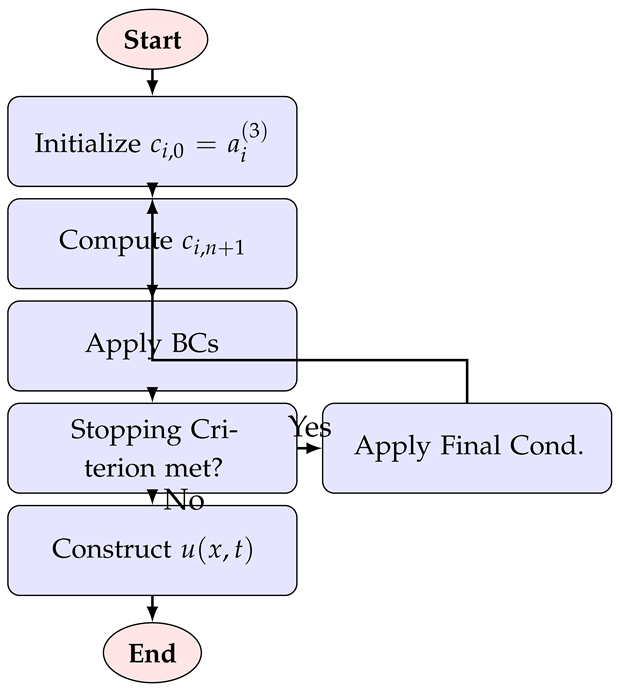
The system of Equations (22)–(26) determines the coefficients recursively, thereby constructing a formal series solution for the fractional differential problem. The algorithm proceeds step by step as follows:
- Step 1
- Initialize the initial coefficients of the series solution using the initial condition : .
- Step 2
- Start the iteration counter with .
- Step 3
- Compute the next coefficients using the recurrence relation derived from the differential equation: .
- Step 4
- Apply the boundary conditions at each iteration level to determine any free parameters in the coefficients.
- Step 5
- Increase the iteration counter: .
- Step 6
- Check the predetermined stopping criterion (specific error tolerance or maximum number of terms N).
- Step 7
- If the stopping criterion is not satisfied, return to Step 3 to continue the process.
- Step 8
- If a final condition is specified, use Equation (26) to determine any remaining coefficients.
- Step 9
- Construct the final solution using all computed coefficients: .
- Step 10
- Terminate the algorithm.
- The flow chart of the algorithm can be demonstrated as follows:
4. Convergence Analysis
This section establishes the convergence of the double fractional power series solution for TSFPEs with variable coefficients and coupled fractional Robin conditions. Using the Banach fixed-point theorem in a weighted Banach space [41], we prove the existence, uniqueness, and local convergence of the formal series, and derive explicit estimates for the convergence radii in , , , and . Applying the Riemann–Liouville integral to (1) and using the initial condition (2) yields the equivalent integral equation
with . Define the solution operator by the right-hand side of (26):
A solution of (1)–(4) corresponds to a fixed point of . Let be fixed. For parameters and define the weighted norm
with . This weighted norm is defined on a coefficient-based space of functions. The growth of the series coefficients () plays a significant role in the convergence analysis of power series. This norm is obtained through gamma functions and geometric weights . If , then the function belongs to the following Banach space:
This norm controls coefficient growth by Gamma-function discounts and geometric weights. From the recurrence relations that guarantee that the distance between successive iterations must strictly shrink, define an iterative scheme with coefficients . The estimate is obtained
where
and C depends on . Note that Equation (31) shows that the absolute difference between the coefficients of two successive iterations is bounded by a contraction factor multiplied by the maximum difference from the preceding iteration. Moreover, it is clear that the factor explicitly depends on the fractional orders (), the boundary parameters (), and the supremum norm of the time-dependent coefficient (). This fundamental inequality implies that the operator acts as a strict contraction mapping. As the indices () grow larger (i.e., moving to higher-order terms in the series), the Gamma functions in the denominator grow significantly faster than those in the numerator.
Theorem 2
(Convergence of the fractional power series). Assume that admit compatible fractional power series expansions. Then there exist constants and such that the operator in (28) is a contraction on equipped with the norm . Consequently,
Proof.
Choose large enough so that
Using the asymptotic behaviour of the Gamma function,
Note that these asymptotic equalities are obtained from the Stirling-type asymptotic formula for the ratio of Gamma functions [42]. We see that for , and sufficiently small, the supremum L becomes less than 1. Hence is a contraction on . The Banach fixed-point theorem then guarantees a unique fixed point ; the convergence of the series and the coefficient bound follow directly from the definition of . From the contraction constant L we obtain the practical estimate
In practice, depend on the fractional orders , the magnitude , the boundary parameters , and the size of the initial and boundary data. The above inequality provides a bound for the convergence radii ( and ) of the spatial and temporal fractional series. This inequality implies that there is an inverse proportion between the domain of convergence and the magnitude of the variable coefficient (), which provides a link between the valid physical domain of the fractional series solution and physical input and initial data. We have thus provided a rigorous convergence foundation for the double fractional power series method applied to the considered class of time-space fractional PDEs. □
5. Illustrative Examples
Example 1.
Consider the time-space fractional PDE with a constant source term:
with the initial condition
and the boundary conditions
where . The operators and denote the Caputo fractional derivatives. Additionally, the final time measurement data
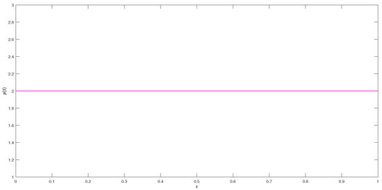
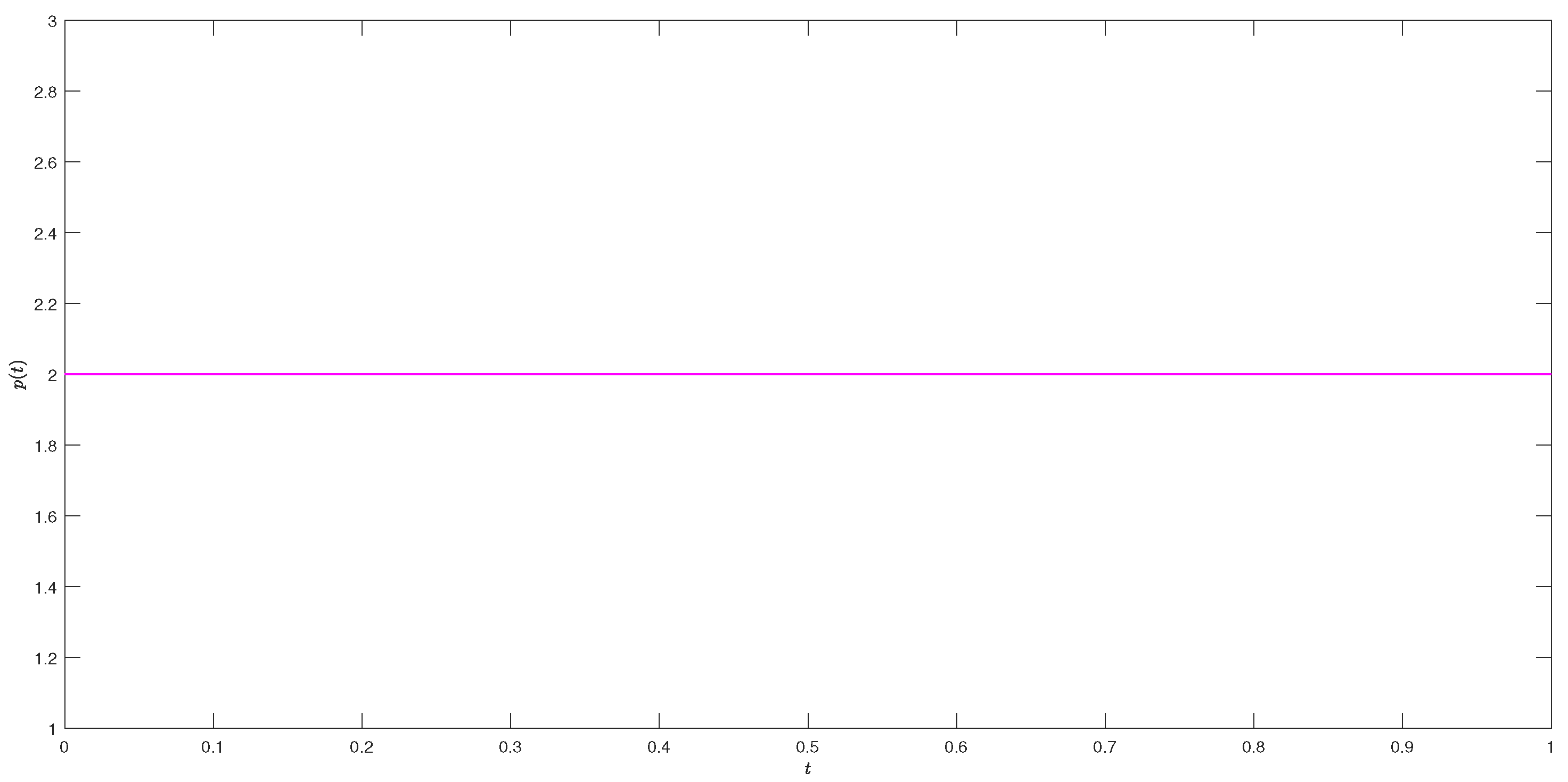
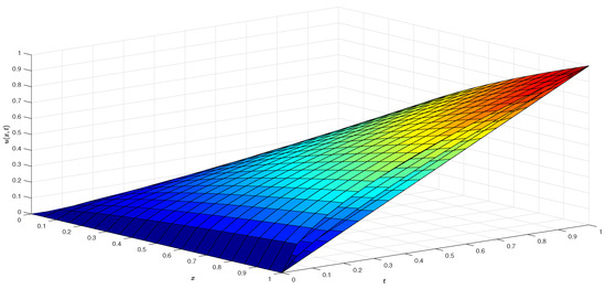
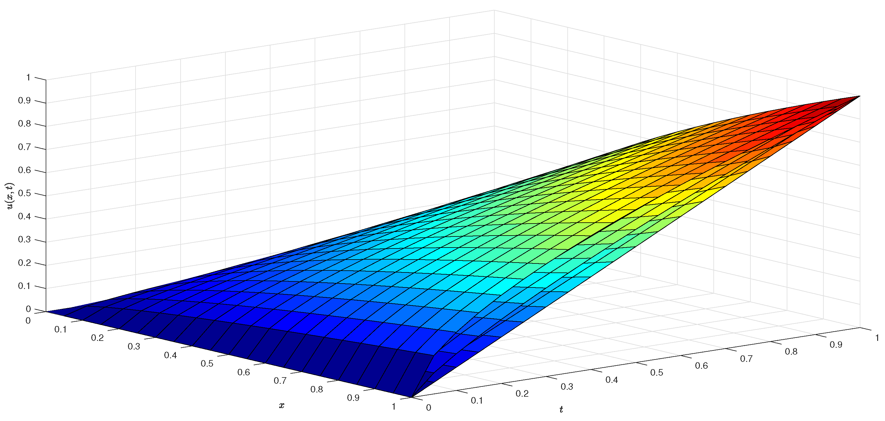
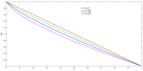
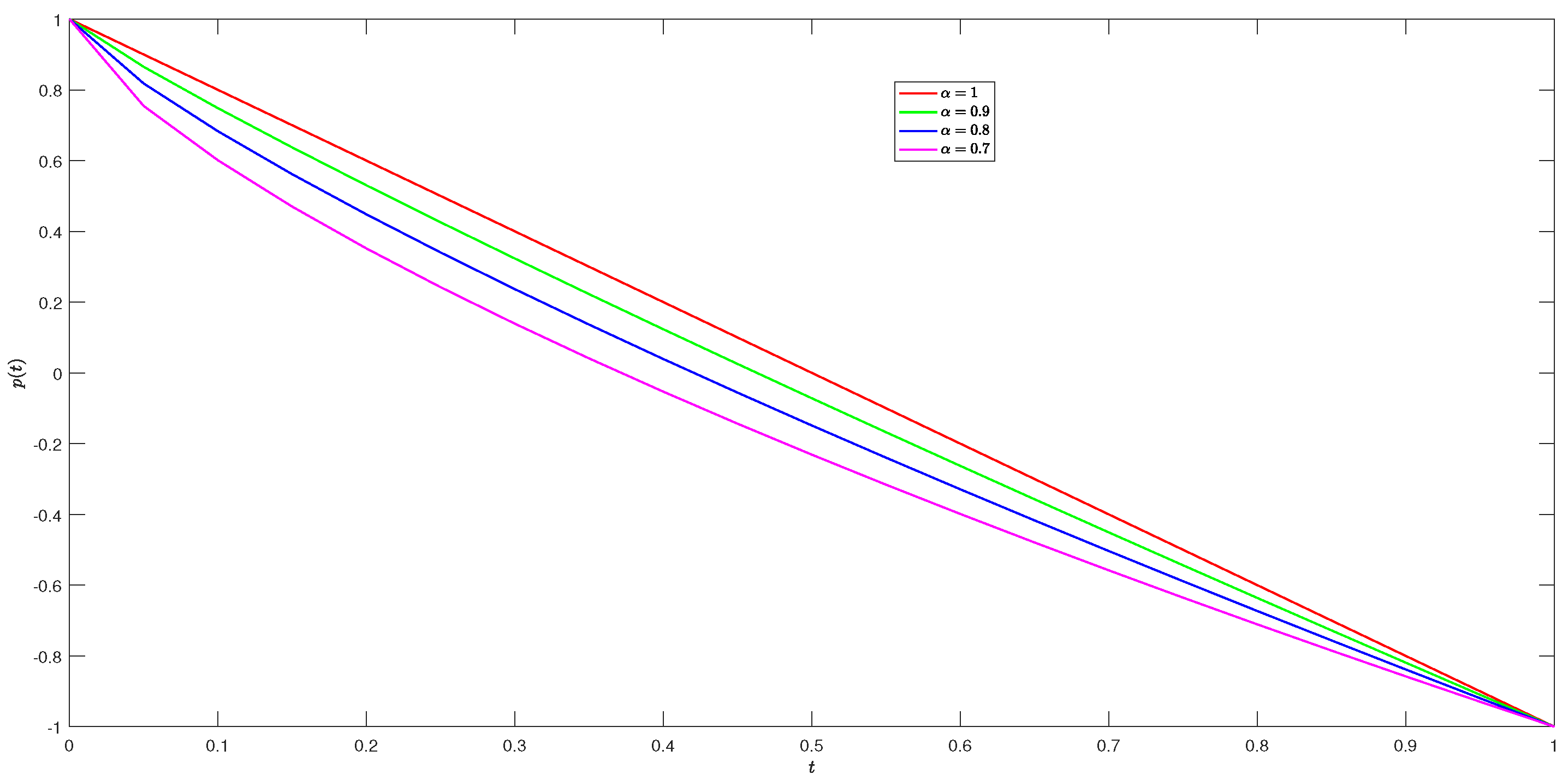
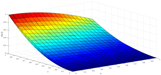
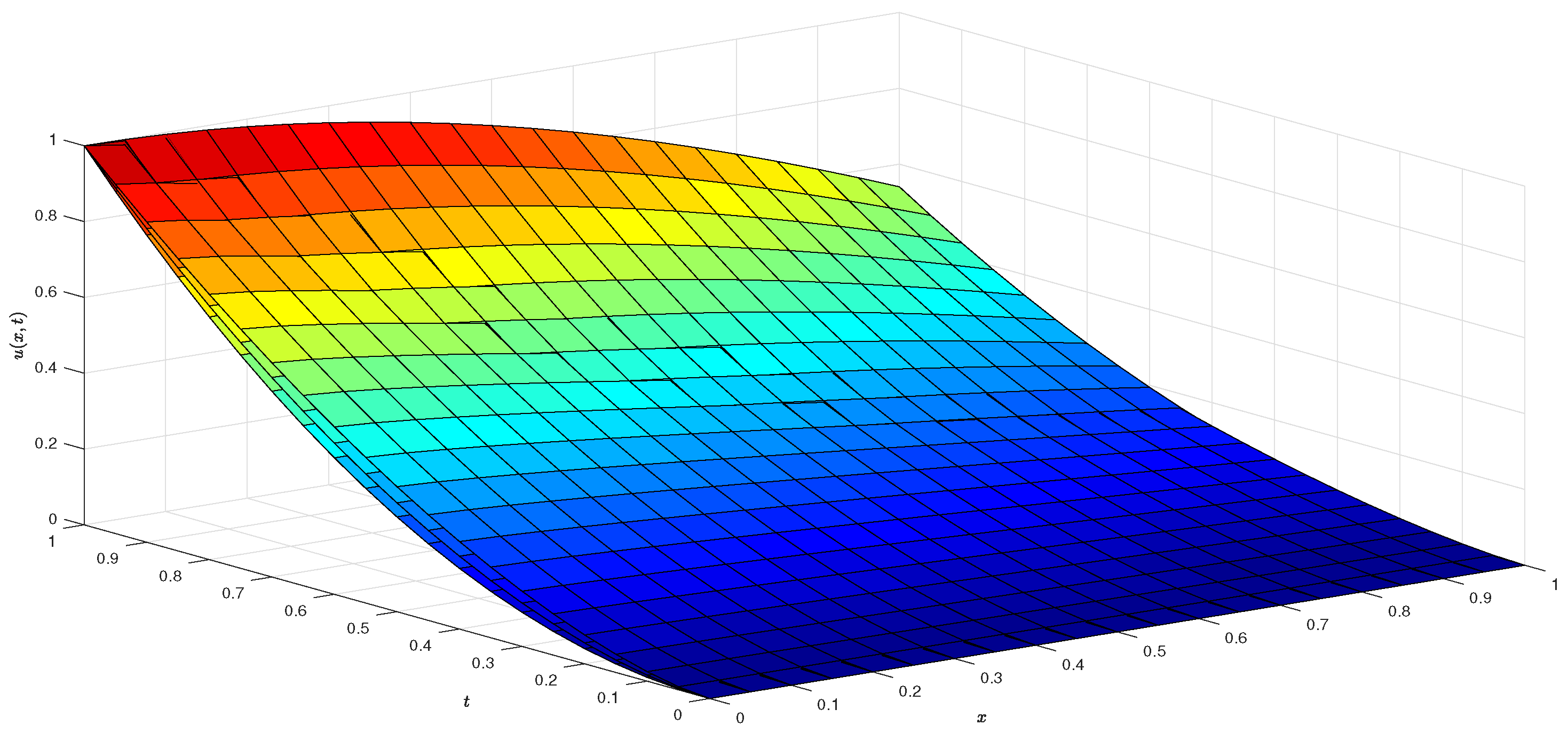
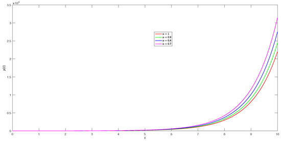
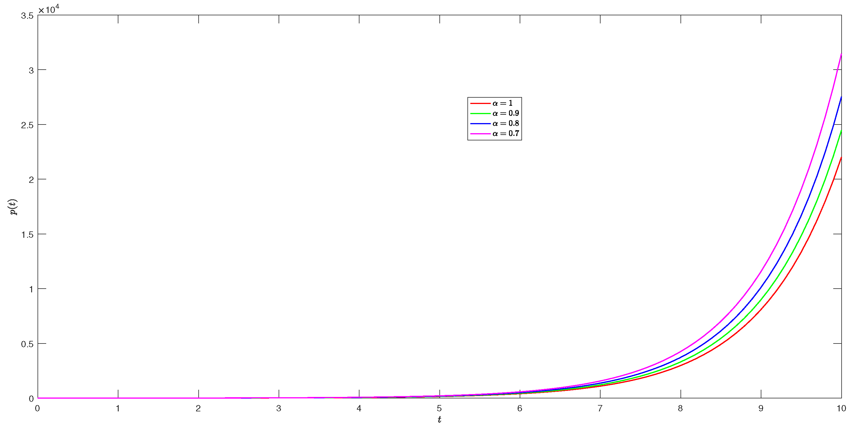
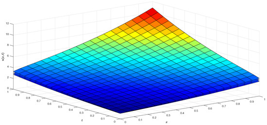
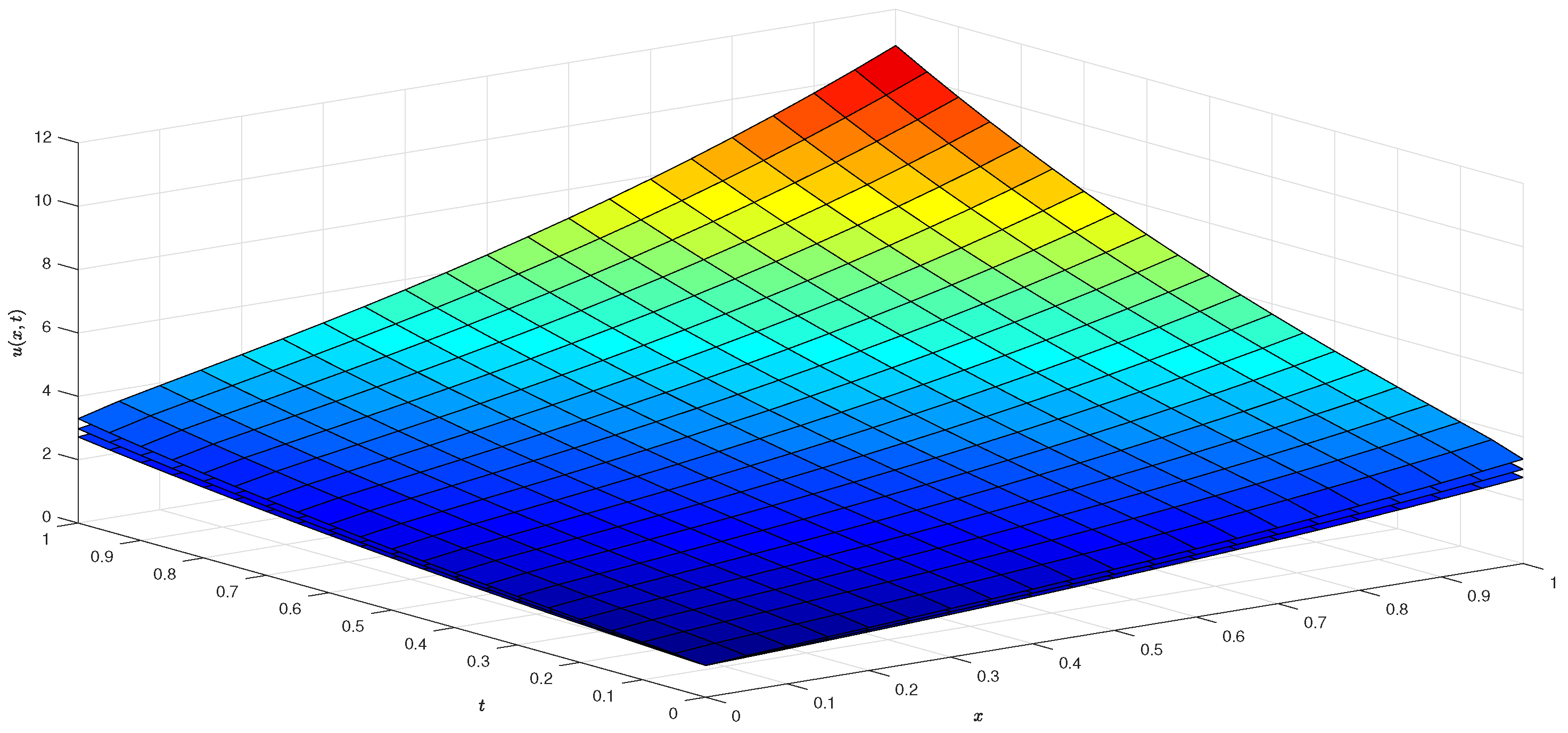
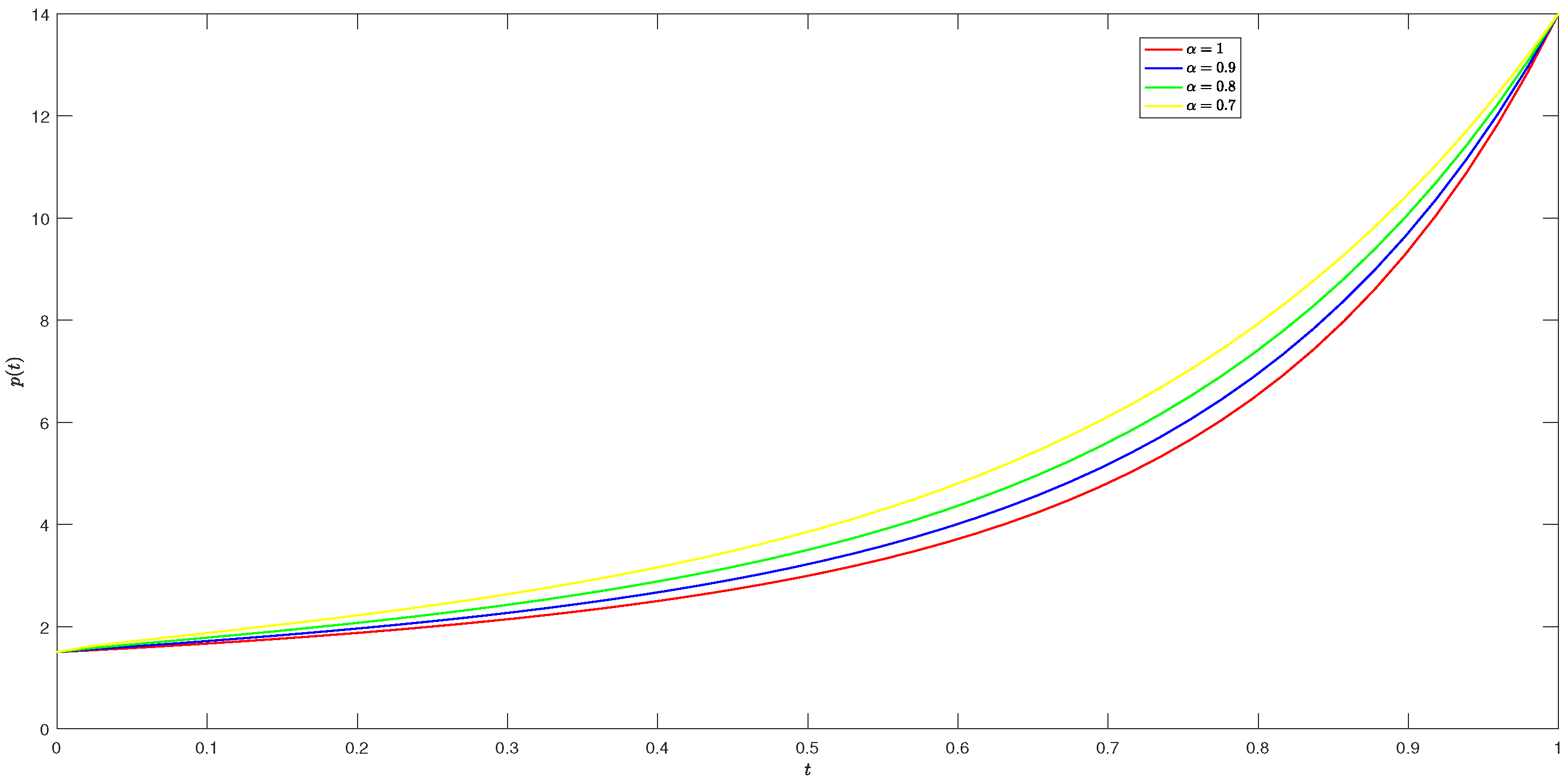
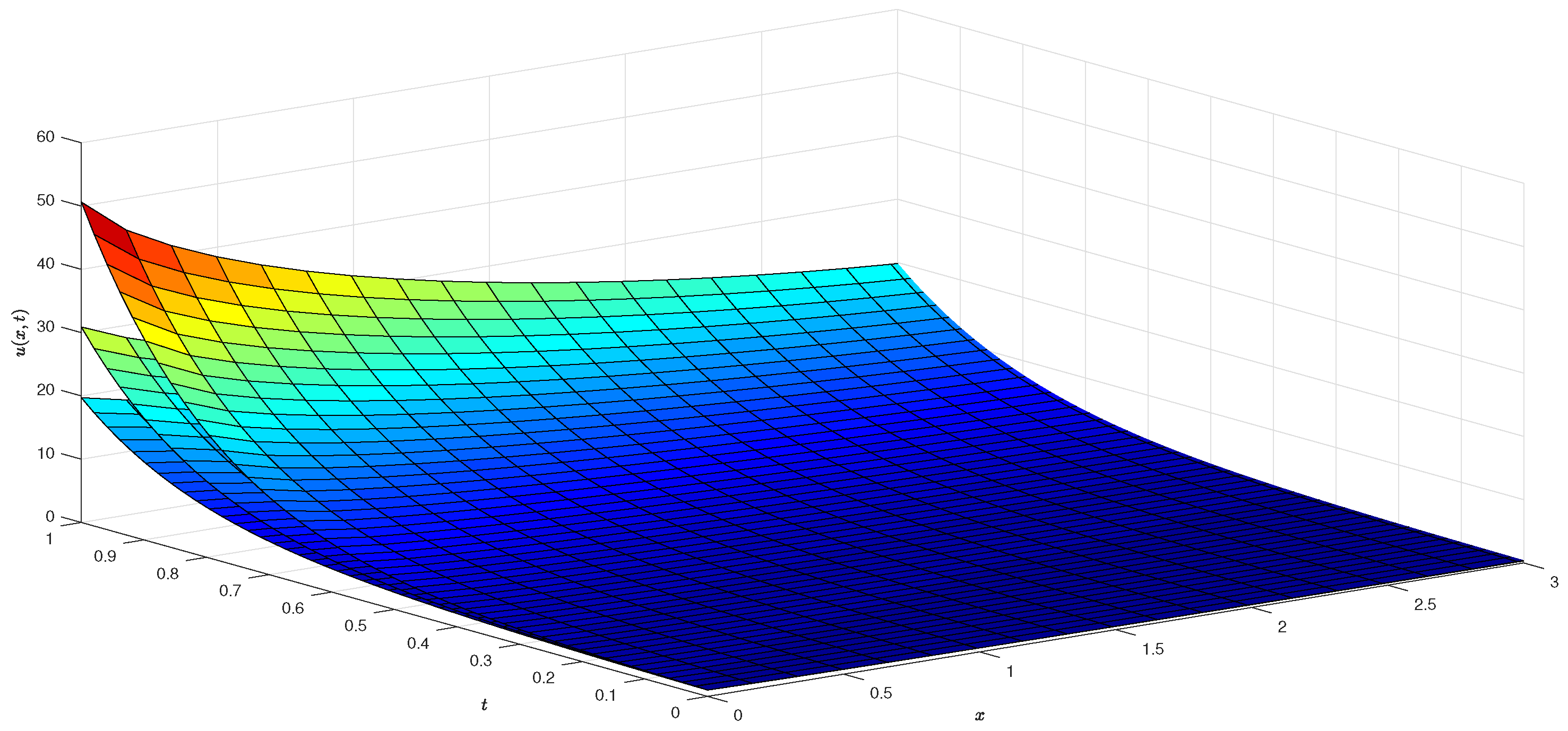
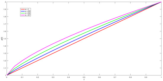
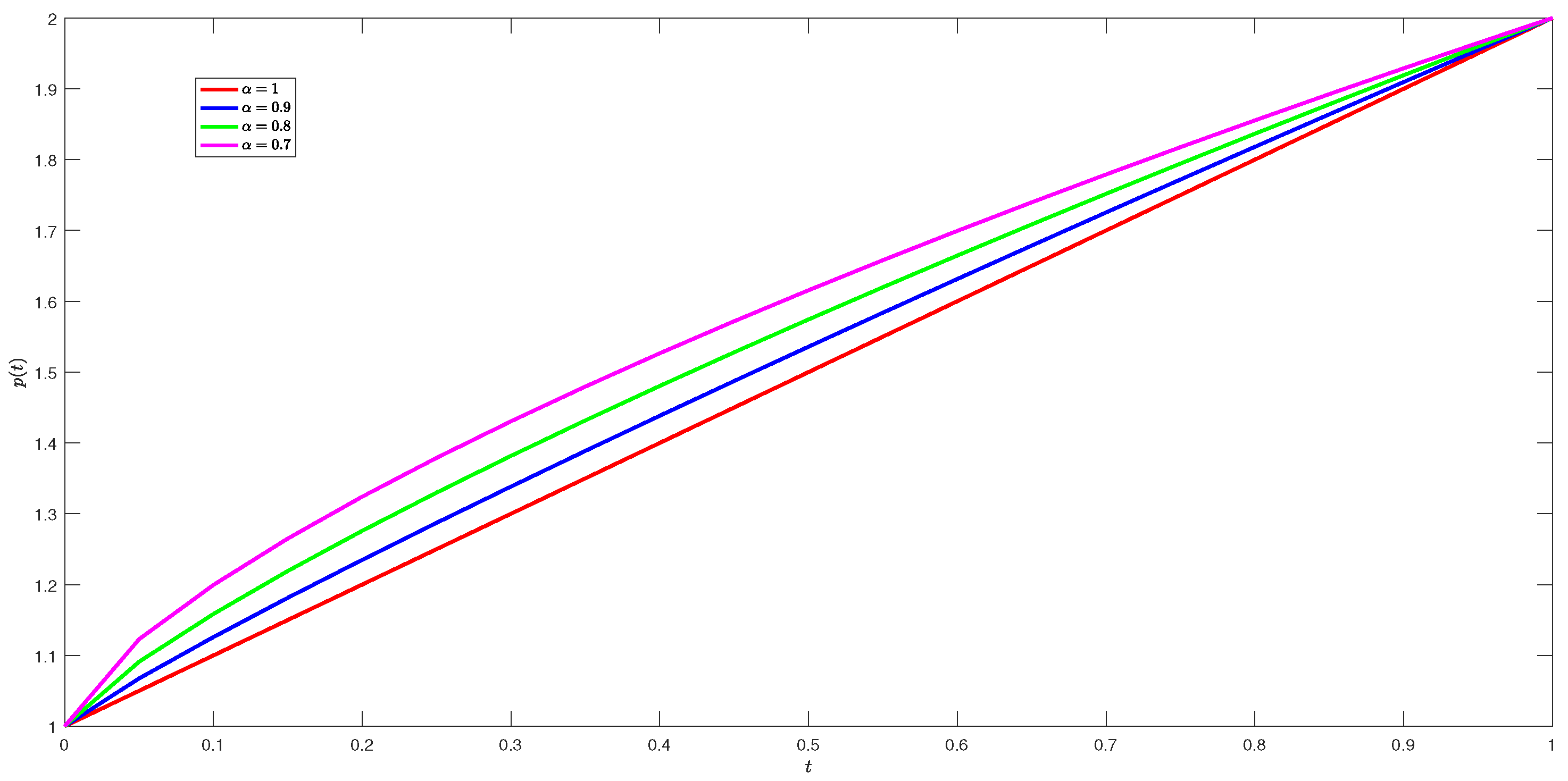
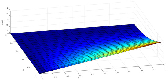
provide an over-specification used in inverse coefficient problems. The exact solutions are and . Figure 1 illustrates the truncated solutions of the time-dependent function in Example 1, highlighting the influence of varying the fractional order α. The visual comparison demonstrates how sub-diffusive memory effects (lower α) alter the temporal evolution compared to the classical case (). Figure 2 presents the truncated solutions for the spatial-temporal field from Example 1, exploring the combined effects of the time-fractional order α and the space-fractional order β. The surface or contour plots reveal how different pairs modify both the diffusion rate and the spatial profile of the solution. Table 1 presents the truncated solutions of Example 1 under equal fractional orders for different spatial positions x and times t.
Figure 1.
Truncated solutions for the function in Example 1 under different values of the fractional order .
Figure 2.
Three-dimensional surface plots for the truncated approach of Example 1, corresponding to the fractional orders equal to .
Table 1.
Truncated solutions for Example 1 with various fractional orders .
Example 2.
Consider the time-space fractional PDE with a constant source term:
with the initial condition
and the boundary conditions
where . The operators and denote the Caputo fractional derivatives. Additionally, the final time measurement data are given as follows:
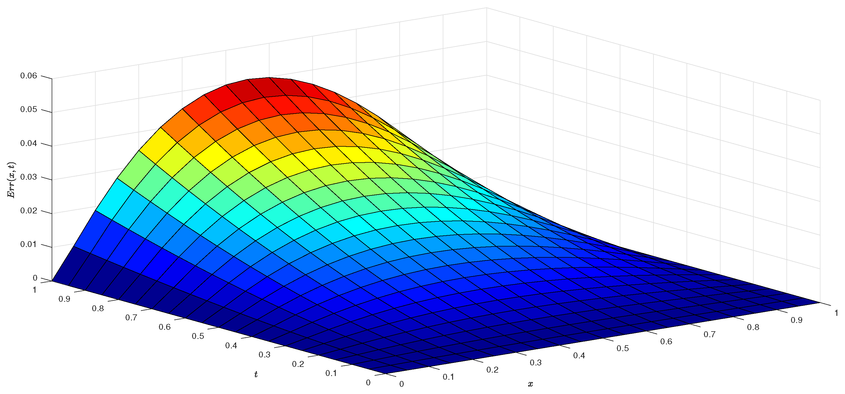
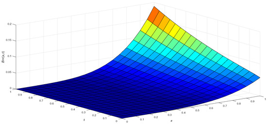
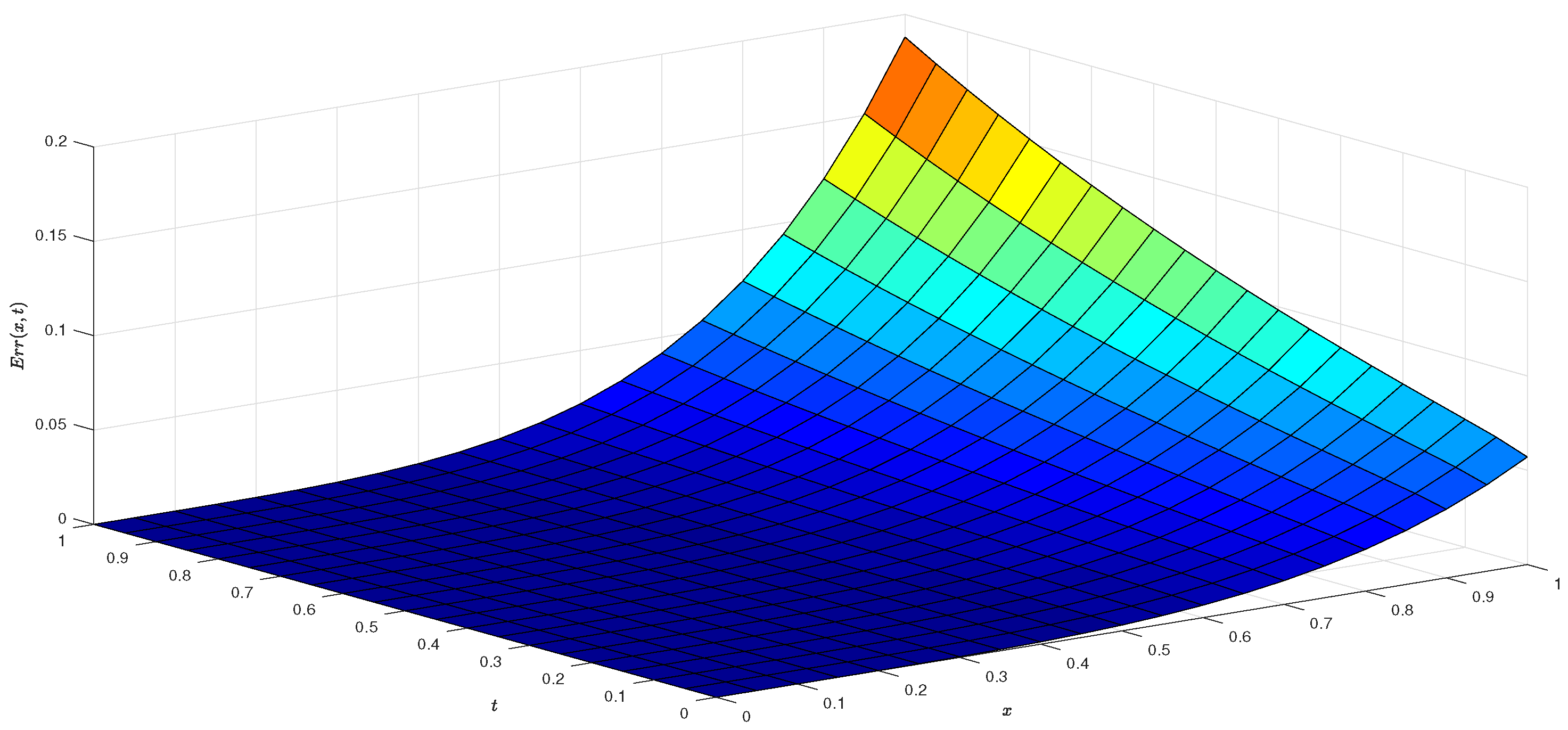
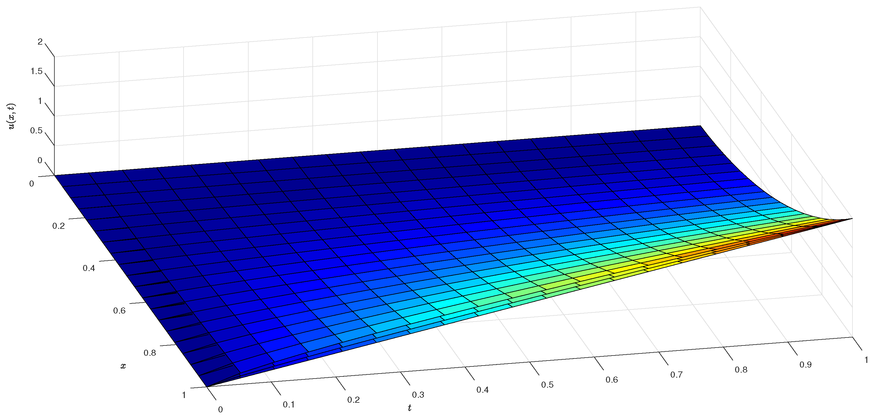
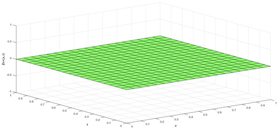
provides an over-specification used in inverse coefficient problems. The exact solutions are and . Figure 3 illustrates the truncated solutions of the time-dependent function in Example 2, highlighting the influence of varying the fractional order α. The visual comparison demonstrates how sub-diffusive memory effects (lower α) alter the temporal evolution compared to the classical case (). Figure 4 presents the truncated solutions for the spatial-temporal field from Example 2, exploring the combined effects of the time-fractional order α and the space-fractional order β. The surface or contour plots reveal how different pairs modify both the diffusion rate and the spatial profile of the solution. Figure 5 presents the 3D distribution of absolute errors between the numerical and exact solutions of Example 2 with , validating the accuracy and consistency of the proposed fractional numerical scheme. The Table 2 presents the truncated solutions of Example 2 under equal fractional orders for different spatial positions x and times t.
Figure 3.
Truncated solutions for the function in Example 2 under various values of .
Figure 4.
Three-dimensional surface plots for the truncated approach of Example 2, corresponding to equal to .
Figure 5.
Three-dimensional visualization of absolute errors for Example 2 with fractional orders .
Table 2.
Truncated solutions for Example 2 with various fractional orders .
Example 3.
Consider the time-space fractional PDE with a constant source term:
with the initial condition
and the boundary conditions
where . The operators and denote the Caputo fractional derivatives. Additionally, final time measurement data
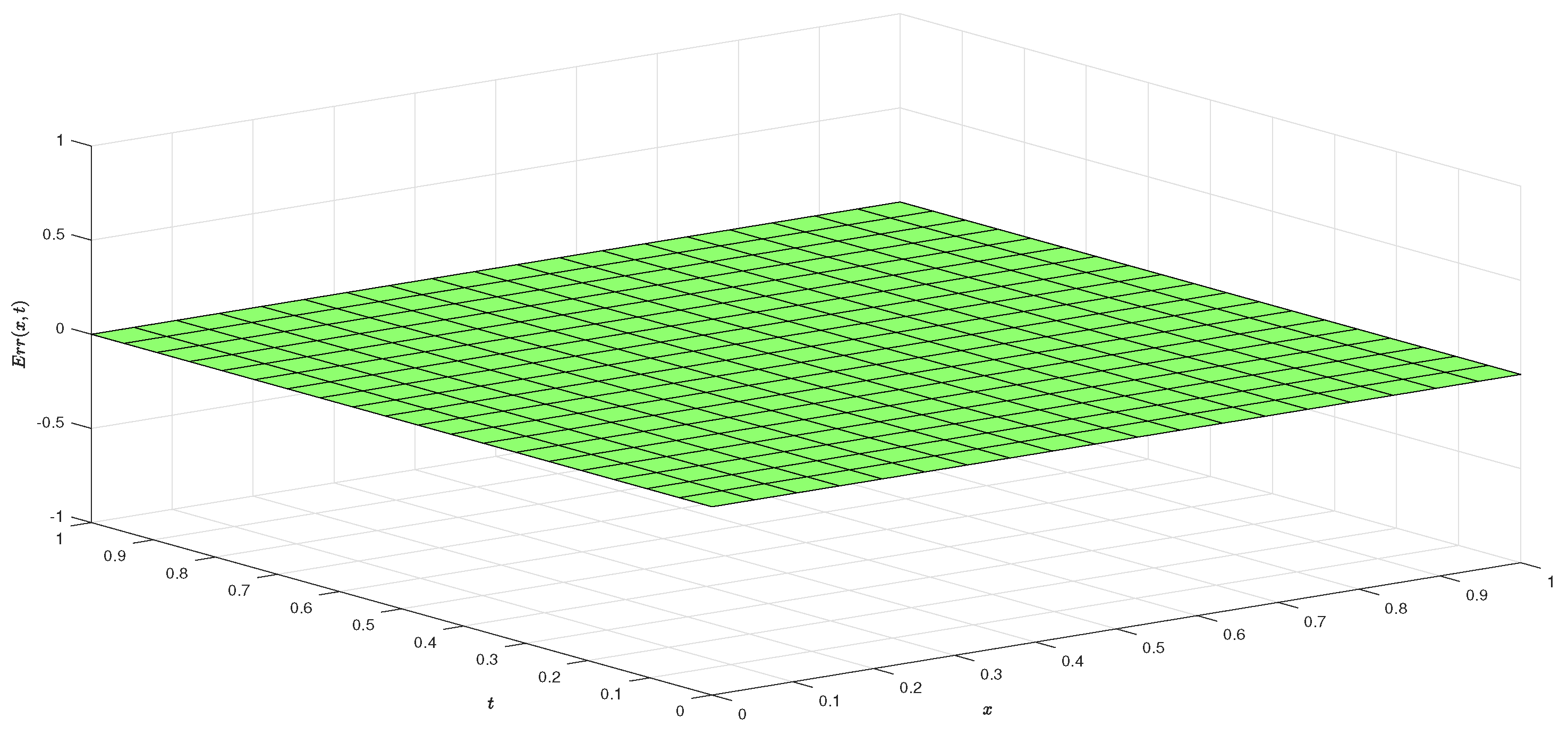
provide an over-specification used in inverse coefficient problems. The exact solutions are and . Figure 6 illustrates the truncated solutions of the time-dependent function in Example 3, highlighting the influence of varying the fractional order α. The visual comparison demonstrates how sub-diffusive memory effects (lower α) alter the temporal evolution compared to the classical case (). Figure 7 presents the truncated solutions for the spatial-temporal field from Example 3, exploring the combined effects of the time-fractional order α and the space-fractional order β. The surface or contour plots reveal how different pairs modify both the diffusion rate and the spatial profile of the solution. Figure 8 presents the 3D distribution of absolute errors between the numerical and exact solutions of Example 3 with , validating the accuracy and consistency of the proposed fractional numerical scheme. Table 3 presents the truncated solutions of Example 3 under equal fractional orders for different spatial positions x and times t.
Figure 6.
Truncated solutions for the function in Example 3 under various values of .
Figure 7.
Three-dimensional surface plots for the truncated approach of Example 3, corresponding to equal to .
Figure 8.
Three-dimensional visualization of absolute errors for Example 3 with fractional parameters .
Table 3.
Truncated solutions for Example 3 with various fractional orders .
Example 4.
Consider the time-space fractional PDE with a constant source term:
with the initial condition
and the boundary conditions
where . The operators and denote the Caputo fractional derivatives. Additionally, the final time measurement data are given as follows:
provides an over-specification used in inverse coefficient problems. The solutions are
and
Figure 9 illustrates the truncated solutions of the time-dependent function in Example 4, highlighting the influence of varying the fractional order α. The visual comparison demonstrates how sub-diffusive memory effects (lower α) alter the temporal evolution compared to the classical case (). Figure 10 presents the truncated solutions for the spatial-temporal field from Example 4, exploring the combined effects of the time-fractional order α and the space-fractional order β. The surface or contour plots reveal how different pairs modify both the diffusion rate and the spatial profile of the solution.
Figure 9.
Truncated solutions for the function in Example 4 under various values of .
Figure 10.
Three-dimensional surface plots for the truncated approach of Example 4, corresponding to equal to .
Example 5.
Consider the time-space fractional PDE with a constant source term:
with the initial condition
and the boundary conditions
where . The operators and denote the Caputo fractional derivatives. Additionally, the final time measurement data are given as follows:
provides an over-specification used in inverse coefficient problems. The exact solutions are and . Figure 11 illustrates the truncated solutions of the time-dependent function in Example 5, highlighting the influence of varying the fractional order α. The visual comparison demonstrates how sub-diffusive memory effects (lower α) alter the temporal evolution compared to the classical case (). Figure 12 presents the truncated solutions for the spatial-temporal field from Example 5, exploring the combined effects of the time-fractional order α and the space-fractional order β. The surface or contour plots reveal how different pairs modify both the diffusion rate and the spatial profile of the solution. Figure 13 presents the 3D distribution of absolute errors between the numerical and exact solutions of Example 5 with , validating the accuracy and consistency of the proposed fractional numerical scheme.
Figure 11.
Truncated solutions for the function in Example 5 under various values of .
Figure 12.
Three-dimensional surface plots for the truncated approach of Example 5, corresponding to equal to .
Figure 13.
Three-dimensional visualization of absolute errors for Example 5 with fractional orders .
6. Conclusions
This study focuses on addressing the inverse coefficient problem for a TSFPE with coupled fractional Robin conditions. By improving and utilizing a fractional power series expansion method, the unknown time-dependent coefficient in the Caputo fractional derivative sense is identified. The primary methodological approach relies on extending the double series expansion framework to fractional powers of both spatial and temporal variables. This study utilizes integer-order double series expansions, which generalize the approach to fractional-order power series. As a result, this extension gives rise to highly accurate results of non-local memory effects. This approach systematically transforms the original inverse problem into a deterministic system of recurrence relations for the expansion coefficients, facilitated by the final time measurement serving as the overdetermination condition. In the finite truncation implementation, the compatibility of multiple constraints is preserved by systematically decoupling the recursive evolution from the boundary and final-time conditions. Specifically, while the initial and boundary conditions govern the local recurrence relations for the series expansion coefficients, the final-time overdetermination condition functions as a global constraint and convergence criterion (Step 6). This ensures that the truncated series solution aligns with the measurement data within the prescribed error tolerance while preventing any over-constraint of the lower-order recurrence scheme.
The work provides a comprehensive and detailed exposition of the mathematical derivations, offering a transparent and replicable analytical pathway for tackling similar non-local problems. A key contribution of this research is the establishment of a rigorous convergence analysis for the proposed series solution. This proof not only substantiates the theoretical validity of the method but also ensures its mathematical consistency and accuracy. Furthermore, the efficacy and practical utility of the methodology were conclusively demonstrated through illustrative numerical examples. These results confirm the method’s high precision, computational stability, and robustness in solving complex inverse coefficient problems involving coupled fractional dynamics and boundary conditions. In summary, this work introduces a viable and effective alternative analytical framework for identifying unknown temporal coefficients in TSFPEs. It advances the analytical toolkit for inverse coefficient problems and provides a solid theoretical foundation with verified practical applicability for future research in fractional calculus and inverse problem analysis. Although the proposed method constructively determines the time-dependent coefficient by means of a uniquely determined system of recurrence relations under overdetermined data, establishing a rigorous analytical uniqueness proof within a broader functional framework remains an open problem. In future research, we will focus on exploring global uniqueness theorems by utilizing generalized spectral methods, Carleman estimates tailored for fractional operators, or energy-estimate techniques adapted to coupled fractional Robin boundary conditions. Moreover, investigating the stability and uniqueness of the reconstruction process under noisy measurement data will be pursued.
Author Contributions
Conceptualization, M.J.H., M.A.B. and A.D.; methodology, M.J.H., M.A.B. and A.D.; software, M.J.H., M.A.B. and A.D.; validation, M.J.H., M.A.B. and A.D.; formal analysis, M.J.H., M.A.B. and A.D.; funding acquisition, M.J.H.; investigation, M.J.H., M.A.B. and A.D.; writing—original draft preparation, M.J.H., M.A.B. and A.D.; writing—review and editing, M.J.H., M.A.B. and A.D.; supervision, M.J.H. All authors have read and agreed to the published version of the manuscript.
Funding
This research received no external funding.
Institutional Review Board Statement
Not applicable.
Informed Consent Statement
Not applicable.
Data Availability Statement
The original contributions presented in this study are included in the article. Further inquiries can be directed to the corresponding authors.
Conflicts of Interest
The authors declare no conflicts of interest.
References
- Eidelman, S.D.; Kochubei, A.N. Cauchy problem for fractional diffusion equations. J. Differ. Equ. 2004, 199, 211–255. [Google Scholar] [CrossRef] [Scilit]
- Kochubei, A.N. Diffusion of fractional order. Differ. Uravn. 1990, 26, 485–492. [Google Scholar]
- Gorenflo, R.; Luchko, Y.F. On solvability of linear fractional differential equations in Banach spaces. Fract. Calc. Appl. Anal. 1999, 2, 163–176. [Google Scholar]
- Kochubei, A.N. The Cauchy problem for fractional-order evolution equations. Differ. Uravn. 1999, 25, 1359–1368. [Google Scholar]
- Hanyga, A. Multidimensional solutions of time-fractional diffusion-wave equations. Proc. R. Soc. Lond. Ser. A Math. Phys. Eng. Sci. 2002, 458, 933–957. [Google Scholar] [CrossRef] [Scilit]
- Pskhu, A.V. Solution of Boundary Value Problems for the Fractional Diffusion Equation by the Green Function Method. Differ. Equ. 2003, 39, 1509–1513. [Google Scholar] [CrossRef] [Scilit]
- Durdiev, D.K.; Nuriddinov, Z.J. Determination of a multidimensional kernel in some parabolic integro-differential equation. J. Sib. Fed. Univ. Math. Phys. 2021, 14, 117–127. [Google Scholar] [CrossRef] [Scilit]
- Durdiev, D.; Durdiev, D. The Fourier spectral method for determining a heat capacity coefficient in a parabolic equation. Turk. J. Math. 2022, 46, 3223–3233. [Google Scholar] [CrossRef] [Scilit]
- Durdiev, D.K. On the uniqueness of kernel determination in the integro-differential equation of parabolic type. J. Samara State Tech. Univ. Ser. Phys. Math. Sci. 2015, 19, 658–666. [Google Scholar]
- Durdiev, D.K.; Zhumaev, Z.Z. Problem of determining a multidimensional thermal memory in a heat conductivity equation. Methods Funct. Anal. Topol. 2019, 25, 219–226. [Google Scholar]
- Durdiev, D.K.; Jumaev, J.J. Memory kernel reconstruction problems in the integro–differential equation of rigid heat conductor. Math. Methods Appl. Sci. 2022, 45, 8374–8388. [Google Scholar] [CrossRef] [Scilit]
- Xiong, T.X.; Hon, C.Y. An inverse problem for fractional diffusion equation in 2-dimensional case: Stability analysis and regularization. J. Math. Anal. Appl. 2012, 393, 185–199. [Google Scholar] [CrossRef] [Scilit]
- Durdiev, D.; Rahmonov, A.A. A multidimensional diffusion coefficient determination problem for the time-fractional equation. Turk. J. Math. 2022, 46, 2250–2263. [Google Scholar] [CrossRef] [Scilit]
- Miller, L.; Yamamoto, M. Coefficient inverse problem for a fractional diffusion equation. Inverse Probl. 2013, 29, 075013. [Google Scholar] [CrossRef] [Scilit]
- Durdiev, D.; Rahmonov, A.A.; Bozorov, Z.R. A two-dimensional diffusion coefficient determination problem for the time-fractional equation. Math. Methods Appl. Sci. 2021, 44, 10753–10761. [Google Scholar] [CrossRef] [Scilit]
- Xiong, X.; Guo, H.; Liu, X. An inverse problem for a fractional diffusion equation. J. Comput. Appl. Math. 2012, 236, 4474–4484. [Google Scholar] [CrossRef] [Scilit]
- Durdiev, D.K. Inverse coefficient problem for the time-fractional diffusion equation. Eurasian J. Math. Comput. Appl. 2022, 9, 44–54. [Google Scholar] [CrossRef] [Scilit]
- Subhonova, Z.A.; Rahmonov, A.A. Problem of determining the time dependent coefficient in the fractional diffusion-wave equation. Lobachevskii J. Math. 2022, 42, 3747–3760. [Google Scholar] [CrossRef] [Scilit]
- Durdiev, U.D. Problem of determining the reaction coefficient in a fractional diffusion equation. Differ. Equ. 2021, 57, 1195–1204. [Google Scholar] [CrossRef] [Scilit]
- Akhundov, A.Y. An inverse problem for linear parabolic equations. Dokl. Akad. Nauk 1983, 39, 3–6. [Google Scholar]
- Ivanchov, N.I.; Pabyrivska, N.V. On determination of two time-dependent coefficients in a parabolic equation. Sib. Math. J. 2002, 43, 323–329. [Google Scholar] [CrossRef] [Scilit]
- Ivanchov, N.I. On the inverse problem of simultaneous determination of thermal conductivity and specific heat capacity. Sib. Math. J. 1994, 35, 547–555. [Google Scholar] [CrossRef] [Scilit]
- Cannon, J.R.; Paul, D.C. Determination of unknown physical properties in heat conduction problems. Int. J. Eng. Sci. 1973, 11, 783–794. [Google Scholar] [CrossRef] [Scilit]
- Huntul, M.J. Uniqueness and CN–Bell Spectral Reconstruction of Three Time-Dependent Coefficients in a Parabolic Inverse Problem with Quadratic Spatial Diffusivity. Mathematics 2026, 14, 1970. [Google Scholar] [CrossRef] [Scilit]
- Nazim, B.K.; Mansur, I.I. An inverse coefficient problem for the heat equation in the case of nonlocal boundary conditions. J. Math. Anal. Appl. 2012, 396, 546–554. [Google Scholar] [CrossRef] [Scilit]
- Changpin, L.; Fanhai, Z. Finite difference methods for fractional differential equations. Int. J. Bifurc. Chaos 2012, 22, 1230014. [Google Scholar] [CrossRef] [Scilit]
- Hussein, M.S.; Lesnic, D. Simultaneous determination of time and space-dependent coefficients in a parabolic equation. Commun. Nonlinear Sci. Numer. Simul. 2016, 33, 194–217. [Google Scholar] [CrossRef] [Scilit]
- El-Ajou, A.; Arqub, O.A.; Zhour, Z.A.; Momani, S. New Results on Fractional Power Series: Theories and Applications. Entropy 2013, 15, 5305–5323. [Google Scholar] [CrossRef] [Scilit]
- Caratelli, D.; Natalini, P.; Ricci, P.E. Fractional differential equations and expansions in fractional powers. Symmetry 2023, 15, 1842. [Google Scholar] [CrossRef] [Scilit]
- Huntul, M.J.; Modanli, M. Numerical approach for solving the inverse problem: A two-dimensional time-fractional boundary value problem. AIMS Math. 2026, 11, 7078–7097. [Google Scholar] [CrossRef] [Scilit]
- Huntul, M.J.; Alagoz, S.; Karaagac, B. Numerical investigation of the time-fractional Fisher equation in physics-based diffusion-reaction systems. AIMS Math. 2026, 11, 15926–15951. [Google Scholar] [CrossRef] [Scilit]
- Derbissaly, B.; Sadybekov, M. Inverse source problem for multi-term time-fractional diffusion equation with nonlocal boundary conditions. AIMS Math. 2024, 9, 9969–9988. [Google Scholar] [CrossRef] [Scilit]
- Podlubny, I. Fractional Differential Equations; Academic Press: New York, NY, USA, 1999. [Google Scholar]
- Kilbas, A.A.; Srivastava, H.M.; Trujillo, J.J. Theory and Applications of Fractional Differential Equations; Elsevier: Amsterdam, The Netherlands, 2006. [Google Scholar]
- Diethelm, K. The Analysis of Fractional Differential Equations an Application-Oriented Exposition Using Differential Operators of Caputo Type; Springer: Berlin/Heidelberg, Germany, 2010. [Google Scholar]
- Caputo, M. Linear models of dissipation whose Q is almost frequency independent—II. Geophys. J. Int. 1967, 13, 529–539. [Google Scholar] [CrossRef] [Scilit]
- Dimache, A.; Groza, G.; Jianu, M.; Iancu, I. Existence and Uniqueness of Solution Represented as Fractional Power Series for the Fractional Advection–Dispersion Equation. Symmetry 2024, 16, 1137. [Google Scholar] [CrossRef] [Scilit]
- Groza, G.; Jianu, M. Functions represented into fractional Taylor series. ITM Web. Conf. 2019, 29, 010117. [Google Scholar] [CrossRef] [Scilit]
- Groza, G.; Jianu, M.; Mierlus-Mazilu, I. Some properties of the functions representable as fractional power series. Mathematics 2024, 12, 961. [Google Scholar] [CrossRef] [Scilit]
- Krantz, S.G.; Parks, H.R. A Primer of Real Analytic Functions; Birkhauser: Boston, MA, USA, 1992. [Google Scholar]
- Kreyszig, E. Introductory Functional Analysis with Applications; Wiley: Hoboken, NJ, USA, 1978. [Google Scholar]
- Olver, F.W.J.; Lozier, D.W.; Boisvert, R.F.; Clark, C.W. NIST Handbook of Mathematical Functions; Cambridge University Press: Cambridge, UK, 2010. [Google Scholar]

Disclaimer/Publisher’s Note: The statements, opinions and data contained in all publications are solely those of the individual author(s) and contributor(s) and not of MDPI and/or the editor(s). MDPI and/or the editor(s) disclaim responsibility for any injury to people or property resulting from any ideas, methods, instructions or products referred to in the content. |
© 2026 by the authors. Licensee MDPI, Basel, Switzerland. This article is an open access article distributed under the terms and conditions of the Creative Commons Attribution (CC BY) license.