Hyperbolic-Tangent Shocks in a Lossy Nonlinear Transmission Line

Abstract

We consider a lossy transmission line with a nonlinear voltage–charge relation. We derive an equation for a traveling front with the charge approaching constant asymptotic values on both sides of the front and solve the inverse problem for this equation exactly. Starting from a prescribed monotonic front profile and a prescribed front speed, we determine the dimensionless squared local sound speed within the front. This quantity is the central object of our analysis and allows us to determine the voltage–charge relation of the transmission line in which the front propagates. The squared sound speed, averaged uniformly over the charge interval spanned by the front, is equal to the squared front speed. We specifically consider fronts with a hyperbolic-tangent profile. All physically admissible fronts of this form are shocks rather than kinks. The voltage–charge relation of the transmission line in which the shock propagates is expressed in terms of the lower incomplete beta function. We also treat a transmission line with a cubic voltage–charge relation and propose an approximate equation that admits the hyperbolic-tangent shock profile as an exact solution. The results of the approximate approach coincide with the broad-shock approximation of the exact inverse solution.

1. Introduction

Nonlinear electrical transmission lines serve both as useful circuit elements and as experimentally accessible models of nonlinear-wave propagation. A voltage-dependent capacitance or current-dependent inductance makes the wave speed depend on the wave amplitude, leading to wave steepening, harmonic generation, solitary waves, and shocks. In an early analysis, Landauer showed that capacitive nonlinearity can transform a periodic signal into an electromagnetic shock and emphasized the role of dissipation in determining the subsequent shock evolution [1]. Electrical networks were later used as controlled lattices for observing soliton propagation and interaction [2]. Soliton-like signals in nonlinear electrical transmission lines have also been constructed, and their linear stability has been analyzed within a modified complex Ginzburg–Landau description [3]. Related multiscale reductions of composite right- and left-handed nonlinear transmission lines predict coupled backward- and forward-propagating vector solitons [4]. Experiments on nonlinear left-handed transmission lines have also demonstrated multistability, period doubling, and the onset of chaotic dynamics at higher input powers [5]. Stationary and traveling localized modes have been observed experimentally and reproduced numerically in driven two-dimensional nonlinear electrical lattices [6]. More generally, the existence, stability, and velocity-dependent dynamics of moving discrete breathers have been investigated in nonlinear $\beta$-Fermi–Pasta–Ulam lattices [7].

Nonlinear transmission lines also have direct technological applications. Varactor-loaded nonlinear transmission lines compress electrical wave fronts and generate very short pulses. Nonlinear $LC$ transmission lines with cubic capacitive nonlinearity have also been proposed as analog-gravity systems, in which a voltage soliton creates an effective event horizon for electromagnetic waves [8]. On the mathematical side, solutions of continuum models with voltage-dependent capacitance, resistance, and leakage conductance have been shown to develop shock discontinuities from sufficiently steep initial data [9]. Thus, nonlinearity supplies the steepening mechanism, while dissipation regularizes the discontinuity into a traveling front of finite width.

Factorization approaches provide an analytical route to solving nonlinear second-order differential equations with polynomial nonlinearities [10]. Related exact-solution and integrability techniques have been applied to the Duffing–van der Pol equation [11]. Kaliappan obtained exact traveling-wave solutions of a nonlinear reaction–diffusion equation [12].

In our previous work, we derived traveling-wave equations for lossy nonlinear transmission lines and obtained an approximate solution for a traveling front with a hyperbolic-tangent profile [13,14]. Here we solve the inverse problem by determining the voltage–charge relation that supports this prescribed profile. The resulting exact relation is expressed in terms of the lower incomplete beta function. In addition, we develop complementary approximate inverse constructions by truncating the large-m expansion of the dimensionless squared local sound speed. We also study the approximate direct problem for a prescribed cubic voltage–charge relation.

2. The Lossy Transmission Line

2.1. The Traveling-Wave Equation

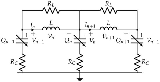
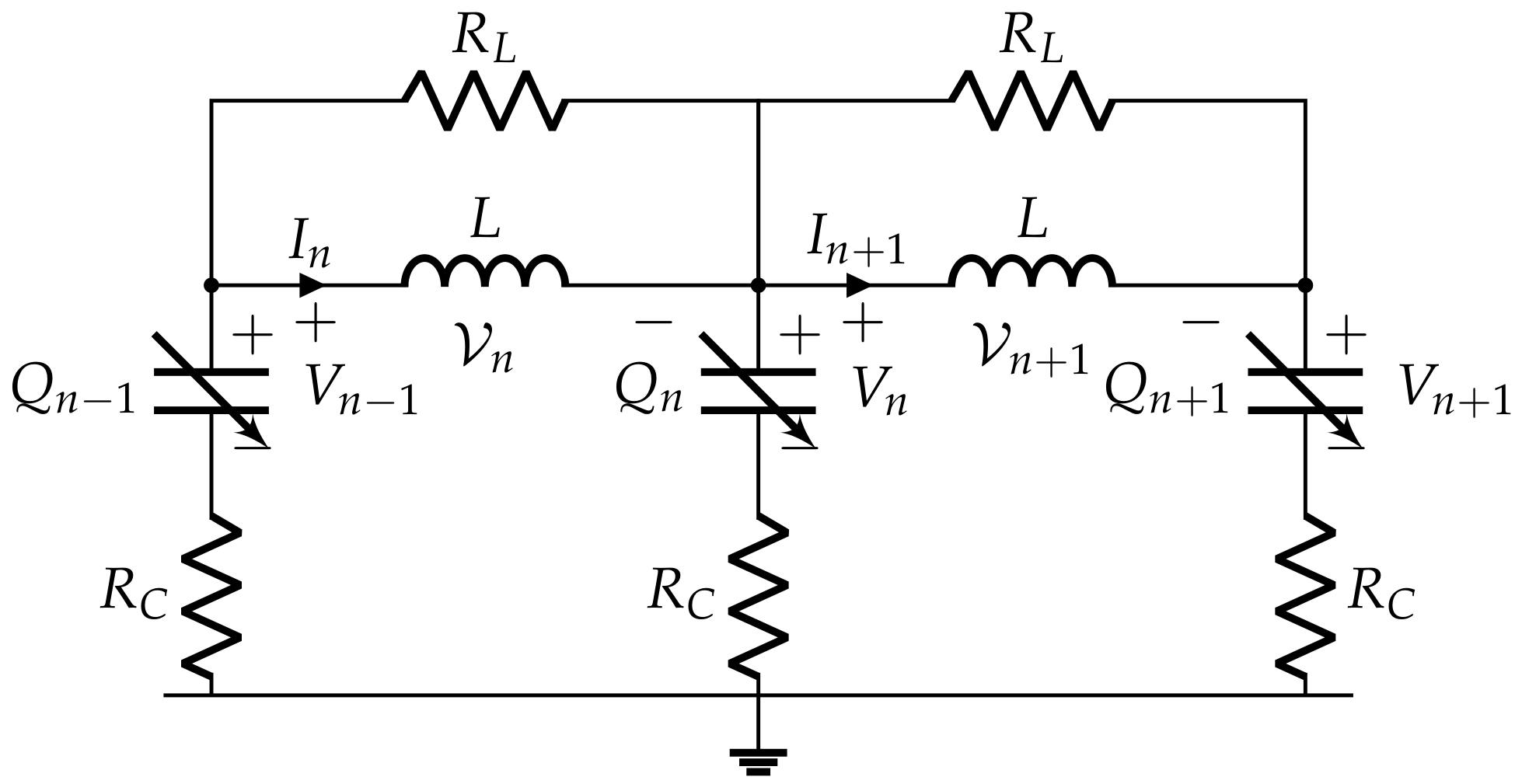
The transmission line studied here, shown in Figure 1, consists of identical inductive branches, each shunted by a resistor $R_L$. Each node is connected to ground through a nonlinear capacitor in series with a resistor $R_C$.

Figure 1. Unit cells of the lossy nonlinear transmission line.

We denote the charge on and the voltage across the nth nonlinear capacitor by $Q_n$ and $V_n$, respectively. The current through the nth inductive branch is denoted by $I_n$, and the voltage across it by ${\mathcal{V}}_n$. Kirchhoff’s laws then give

$$\begin{array}{cc}\hfill {\displaystyle \frac{d{Q}_n}{dt}}& =I_n-I_{n+1}+{\displaystyle \frac{1}{R_L}}\left({\mathcal{V}}_n-{\mathcal{V}}_{n+1}\right),\hfill \\ \hfill {\mathcal{V}}_{n+1}& =V_n-V_{n+1}+R_C{\displaystyle \frac{d}{dt}}\left(Q_n-Q_{n+1}\right).\hfill \end{array}$$

(1)

We restrict the analysis that follows to transmission lines with a linear inductance

$${\mathcal{V}}_n=L{\displaystyle \frac{d{I}_n}{dt}},$$

(2)

where L is a constant, and a nonlinear voltage–charge relation $V_n=V\left(Q_n\right)$.

In the continuum approximation, we replace the discrete index n by the continuous coordinate z, measured in units of the transmission-line period, and approximate the finite differences on the right-hand sides by first derivatives with respect to z. In this approximation, Equation (1) takes the form

$$\begin{array}{cc}\hfill {\mathit{\partial }}_{t}Q& =-{\mathit{\partial }}_{z}I-{\displaystyle \frac{L}{R_L}}{\mathit{\partial }}_{zt}^{2}I,\hfill \end{array}$$

(3)

$$\begin{array}{cc}\hfill L{\mathit{\partial }}_{t}I& =-{\mathit{\partial }}_{z}V-R_C{\mathit{\partial }}_{zt}^{2}Q.\hfill \end{array}$$

(4)

We consider traveling waves for which all quantities depend on the single variable $t-z/U$, where U is the wave speed. We take $U>0$, corresponding to propagation in the positive z direction. For such waves, Equations (3) and (4) reduce to ordinary differential equations. Introducing the dimensionless time

$$\theta ={\displaystyle \frac{R_L}{L}}\left(t-{\displaystyle \frac{z}{U}}\right),$$

(5)

and integrating Equations (3) and (4) once, we obtain

$$\begin{array}{cc}\hfill {\displaystyle \frac{dI}{d\theta }}+I-UQ& =I_A,\hfill \end{array}$$

(6)

$$\begin{array}{cc}\hfill {\displaystyle \frac{1}{C}}{\displaystyle \frac{dQ}{d\theta }}+V\left(Q\right)-ULI& =V_A.\hfill \end{array}$$

(7)

Here $I_A$ and $V_A$ are integration constants, and we introduce the effective capacitance $C=L/\left(R_L{R}_C\right)$, which we treat as prescribed throughout. Solving Equation (7) for I and substituting the result into Equation (6), we obtain a closed equation for Q:

$$\begin{array}{cc}\hfill {\displaystyle \frac{d^{2}Q}{d{\theta }^2}}& +\left[1+w\left(Q\right)\right]{\displaystyle \frac{dQ}{d\theta }}=F\left(Q\right),\hfill \end{array}$$

(8)

$$\begin{array}{cc}\hfill w\left(Q\right)& =C{\displaystyle \frac{dV\left(Q\right)}{dQ}},\hfill \end{array}$$

(9)

$$\begin{array}{cc}\hfill F\left(Q\right)& =WQ-C\left[V\left(Q\right)-V_A\right],\hfill \end{array}$$

(10)

$$\begin{array}{cc}\hfill W& =LC{U}^2.\hfill \end{array}$$

(11)

(We redefined the integration constant $V_A+UL{I}_A\to V_A$.) Note that

$$w\left(Q\right)=LC{u}^2\left(Q\right),$$

(12)

where $u\left(Q\right)$ is the sound speed of small-amplitude, long-wavelength (sound) waves on a homogeneous background with charge Q [13]. The dimensionless squared sound speed w will be the central object of our analysis.

Equation (8) admits a mechanical interpretation as the motion of a unit-mass particle with coordinate Q and time $\theta$ in the effective potential $\Pi \left(Q\right)$ defined by

$$F\left(Q\right)=-{\displaystyle \frac{d\Pi \left(Q\right)}{dQ}},$$

(13)

and subject to viscous damping with the coordinate-dependent coefficient $1+w\left(Q\right)$. The mechanical problem is constrained by the electrodynamics of the transmission line: the same constitutive law $V\left(Q\right)$ determines the effective potential and the damping coefficient.

2.2. Kinks and Shocks

We impose the traveling-front boundary conditions

$$\underset{\theta \to -\infty }{\lim }Q\left(\theta \right)=Q_1,\underset{\theta \to +\infty }{\lim }Q\left(\theta \right)=Q_2.$$

(14)

Thus, $Q_1$ and $Q_2$ characterize the asymptotic states before and after the passage of the front, respectively. The boundary conditions require

$$F\left(Q_1\right)=F\left(Q_2\right)=0.$$

(15)

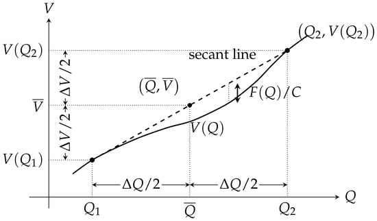
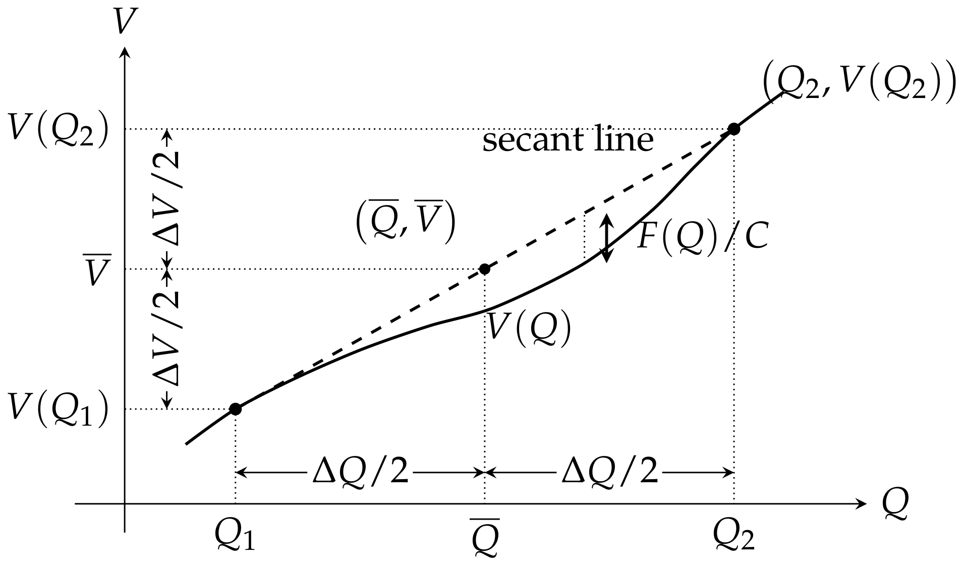
Note that $F\left(Q\right)$ is the signed vertical displacement in the Q–V plane from the voltage–charge curve $V\left(Q\right)$ to the secant line joining $\left(Q_1,V\left(Q_1\right)\right)$ and $\left(Q_2,V\left(Q_2\right)\right)$. Figure 2 illustrates this geometrical interpretation. We introduce

$$\begin{array}{cc}\hfill \Delta Q& =Q_2-Q_1,\hfill \\ \hfill \overline{Q}& ={\displaystyle \frac{Q_2+Q_1}{2}},\hfill \\ \hfill \Delta V& =V\left(Q_2\right)-V\left(Q_1\right),\hfill \\ \hfill \overline{V}& ={\displaystyle \frac{V\left(Q_2\right)+V\left(Q_1\right)}{2}};\hfill \end{array}$$

(16)

in this notation, the horizontal and vertical distances from the midpoint to the endpoints are $\Delta Q/2$ and $\Delta V/2$, respectively.

Figure 2. Geometrical interpretation of the force $F\left(Q\right)$. The dashed line is the secant through the asymptotic states $\left(Q_1,V\left(Q_1\right)\right)$ and $\left(Q_2,V\left(Q_2\right)\right)$. The signed vertical separation between the secant and the nonlinear voltage–charge curve is $F\left(Q\right)/C$. In the present notation the distances from the midpoint $\left(\overline{Q},\overline{V}\right)$ to the endpoints are $\Delta Q/2$ and $\Delta V/2$.

In the mechanical analogy, the fictitious particle moves through the potential landscape from the equilibrium position at $Q=Q_1$ to that at $Q=Q_2$. Hence $Q_1$ must be a local maximum of $\Pi \left(Q\right)$, so that the particle can depart from it. If the trajectory terminates at a local maximum at $Q=Q_2$, the traveling front is a kink; if it terminates at a local minimum, the front is a shock. These maximum and minimum conditions can be conveniently presented in terms of the dimensionless squared sound speed:

$$\begin{array}{cc}\hfill w\left(Q_1\right)& <W,\hfill \end{array}$$

(17)

$$\begin{array}{cc}\hfill w\left(Q_2\right)& >W\left(\mathrm{shock}\right)\hfill \end{array}$$

(18)

$$\begin{array}{cc}\hfill w\left(Q_2\right)& <W\left(\mathrm{kink}\right).\hfill \end{array}$$

(19)

A degenerate case

$$w\left(Q_2\right)=W$$

(20)

demands a more detailed analysis. Thus, the traveling front is supersonic relative to the asymptotic state ahead of it. Relative to the asymptotic state behind it, the front is also supersonic for a kink but subsonic for a shock [13,15]. Further details of this dichotomy are given in Section 6.

From the boundary conditions, we obtain

$$\begin{array}{cc}\hfill W& =C{\displaystyle \frac{\Delta V}{\Delta Q}},\hfill \end{array}$$

(21)

$$\begin{array}{cc}\hfill V_A& =\overline{V}-\overline{Q}{\displaystyle \frac{\Delta V}{\Delta Q}},\hfill \end{array}$$

(22)

and Equation (8) becomes

$${\displaystyle \frac{d^{2}Q}{d{\theta }^2}}+\left[1+w\left(Q\right)\right]{\displaystyle \frac{dQ}{d\theta }}=W\left(Q-\overline{Q}\right)-C\left[V\left(Q\right)-\overline{V}\right].$$

(23)

We introduce the dimensionless charge v by

$$Q-\overline{Q}={\displaystyle \frac{\Delta Q}{2}}v,v\in [-1,1],$$

(24)

and Equation (8) becomes

$${\displaystyle \frac{d^{2}v}{d{\theta }^2}}+\left[1+w\left(v\right)\right]{\displaystyle \frac{dv}{d\theta }}={\displaystyle \frac{2W}{\Delta V}}\left[V^{\mathrm{lin}}\left(v\right)-V\left(v\right)\right],$$

(25)

where

$$V^{\mathrm{lin}}\left(v\right)=\overline{V}+{\displaystyle \frac{\Delta V}{2}}v.$$

(26)

If the slope function

$$S\left(\theta \right)={\displaystyle \frac{dv}{d\theta }}$$

(27)

is strictly positive for $\theta \in (-\infty ,\infty )$, we can invert the function $\theta \left(v\right)$ and regard v as the new independent variable and $\theta$ as the new dependent variable. We also introduce the exponential variable $\Theta$, defined by

$$\Theta =-e^{-\theta }.$$

(28)

In the new variables

$$\begin{array}{cc}\hfill S\left(v\right)& ={\displaystyle \frac{dv}{d\theta }}=-{\displaystyle \frac{\Theta \left(v\right)}{{\Theta }^{{\displaystyle \prime }}\left(v\right)}},\hfill \\ \hfill S^{{\displaystyle \prime }}\left(v\right)& ={\displaystyle \frac{\Theta \left(v\right){\Theta }^{{\displaystyle ″}}\left(v\right)}{{\left[{\Theta }^{{\displaystyle \prime }}\left(v\right)\right]}^2}}-1,\hfill \end{array}$$

(29)

and Equations (25) and (9) can be written as a system of two equations for two unknown functions $\Theta \left(v\right)$ and $w\left(v\right)$:

$$\begin{array}{cc}\hfill & {\left[{\displaystyle \frac{w\left(v\right)+S^{{\displaystyle \prime }}\left(v\right)}{{\Theta }^{{\displaystyle \prime }}\left(v\right)}}\right]}^{{\displaystyle \prime }}=-{\displaystyle \frac{W}{\Theta \left(v\right)}},\hfill \end{array}$$

(30)

$$\begin{array}{cc}\hfill & V\left(v\right)=V^{\mathrm{lin}}\left(v\right)+{\displaystyle \frac{\Delta V}{2W}}{\displaystyle \frac{\Theta \left(v\right)}{{\Theta }^{{\displaystyle \prime }}\left(v\right)}}\left[w\left(v\right)+S^{{\displaystyle \prime }}\left(v\right)+1\right].\hfill \end{array}$$

(31)

Throughout, a prime denotes differentiation with respect to the displayed argument.

3. The Inverse Problem

We now formulate our inverse-design approach. The quantities $\overline{Q}$ and $\Delta Q$ are considered to be prescribed. We prescribe the dimensionless squared front speed W and a monotonic front profile $\Theta \left(v\right)$, satisfying the boundary conditions

$$\underset{v\to -1}{\lim }\Theta \left(v\right)=-\infty ,\Theta \left(1\right)=0.$$

(32)

Equation (30) then becomes a first-order linear differential equation for the dimensionless squared local sound speed $w_W\left(v\right)$, which can be integrated by quadrature, and the solution compatible with a finite value of $w_W(-1)$ is

$$w_W\left(v\right)=-W{\Theta }^{{\displaystyle \prime }}\left(v\right){\int }_{-1}^v{\displaystyle \frac{ds}{\Theta \left(s\right)}}-S^{{\displaystyle \prime }}\left(v\right).$$

(33)

The physical admissibility condition

$$0<w_W\left(v\right)<\infty v\in [-1,1]$$

(34)

is the additional condition to be imposed on the prescribed front profile $\Theta \left(v\right)$.

From Equations (31) and (33) we obtain the voltage–charge relation

$$V\left(v\right)=V^{\mathrm{lin}}\left(v\right)-{\displaystyle \frac{\Delta V}{2}}\Theta \left(v\right)\left[{\int }_{-1}^v{\displaystyle \frac{ds}{\Theta \left(s\right)}}-{\displaystyle \frac{1}{W{\Theta }^{{\displaystyle \prime }}\left(v\right)}}\right],$$

(35)

provided $\overline{V}$ and $\Delta V$ are also prescribed.

It follows from Equation (33) that the dimensionless squared sound speed, averaged uniformly over the charge interval spanned by the front, is equal to the dimensionless squared front speed:

$${\displaystyle \frac{1}{2}}{\int }_{-1}^1{w}_W\left(v\right)dv=W.$$

(36)

In fact, integrating Equation (33) from $-1$ to 1 gives two separate integrals:

$$\begin{array}{cc}\hfill & {\int }_{-1}^1{w}_W\left(v\right)dv=J_1-J_2,\hfill \end{array}$$

(37)

$$\begin{array}{cc}\hfill J_1& =-W{\int }_{-1}^1{\Theta }^{{\displaystyle \prime }}\left(v\right)\left({\int }_{-1}^v{\displaystyle \frac{ds}{\Theta \left(s\right)}}\right)dv=-W{\int }_{-1}^1{\displaystyle \frac{1}{\Theta \left(s\right)}}\left({\int }_s^1{\Theta }^{{\displaystyle \prime }}\left(v\right)dv\right)ds\hfill \\ \hfill & =-W{\int }_{-1}^1{\displaystyle \frac{1}{\Theta \left(s\right)}}{\left.\Theta \left(v\right)\right|}_s^{1}ds=2W.\hfill \end{array}$$

(38)

$$\begin{array}{cc}\hfill J_2& ={\int }_{-1}^1{S}^{{\displaystyle \prime }}\left(v\right)dv=S\left(1\right)-S(-1)=0.\hfill \end{array}$$

(39)

The last equality follows from Equation (27) and the asymptotic boundary conditions for the front.

The Boundary Conditions

Let us write down Equation (33) in terms of $v\left(\theta \right)$ rather than $\Theta \left(v\right)$

$$w_W\left(\theta \right)={\displaystyle \frac{W{e}^{-\theta }}{v^{\prime }\left(\theta \right)}}{\int }_{-\infty }^{\theta }{e}^{\tau }{v}^{\prime }\left(\tau \right)d\tau -{\displaystyle \frac{v^{″}\left(\theta \right)}{v^{\prime }\left(\theta \right)}}.$$

(40)

To obtain limiting behavior of $w_W\left(\theta \right)$ at the leading edge we may use L’Hôpital’s rule, which gives

$$\underset{\theta \to -\infty }{\lim }{w}_W\left(\theta \right)=\underset{\theta \to -\infty }{\lim }\left[{\displaystyle \frac{W}{1+\frac{v^{″}\left(\theta \right)}{v^{\prime }\left(\theta \right)}}}-{\displaystyle \frac{v^{″}\left(\theta \right)}{v^{\prime }\left(\theta \right)}}\right].$$

(41)

Assuming that $v^{\prime }\left(\theta \right)$ monotonically increases with $\theta$ at large negative $\theta$, we have

$$\underset{\theta \to -\infty }{\lim }{\displaystyle \frac{v^{″}\left(\theta \right)}{v^{\prime }\left(\theta \right)}}\ge 0.$$

(42)

Leaving the degenerate case, when the limit in the previous equation is equal to zero for the future analysis, here we consider only the case of the positive limit. In this case the condition (17) is satisfied automatically.

Suppose that when $\theta \to -\infty$

$$1+v\left(\theta \right)\sim A{e}^{\theta /m_{-}},A>0,m_{-}>0.$$

(43)

Then from Equation (41) we obtain

$$\underset{\theta \to -\infty }{\lim }{w}_W\left(\theta \right)={\displaystyle \frac{m_{-}W}{m_{-}+1}}-{\displaystyle \frac{1}{m_{-}}}.$$

(44)

The boundary condition

$$\underset{\theta \to -\infty }{\lim }{w}_W\left(\theta \right)>0$$

(45)

is thus equivalent to

$$W>{\displaystyle \frac{m_{-}+1}{m_{-}^2}}.$$

(46)

Now consider the trailing edge of the front. The limit ${\lim }_{\theta \to \infty }{w}_W\left(\theta \right)$ is finite, when the integral in Equation (40) diverges and

$$\underset{\theta \to \infty }{\lim }{\displaystyle \frac{e^{-\theta }}{v^{\prime }\left(\theta \right)}}=0.$$

(47)

We again may use L’Hôpital’s rule to obtain

$$\underset{\theta \to \infty }{\lim }{w}_W\left(\theta \right)=\underset{\theta \to \infty }{\lim }\left[{\displaystyle \frac{W}{1+\frac{v^{″}\left(\theta \right)}{v^{\prime }\left(\theta \right)}}}-{\displaystyle \frac{v^{″}\left(\theta \right)}{v^{\prime }\left(\theta \right)}}\right].$$

(48)

Assuming that $v^{\prime }\left(\theta \right)$ monotonically decreases with $\theta$ at large positive $\theta$, we have

$$\underset{\theta \to \infty }{\lim }{\displaystyle \frac{v^{″}\left(\theta \right)}{v^{\prime }\left(\theta \right)}}\le 0,$$

(49)

Again leaving the degenerate case, when the limit in the previous equation is equal to zero for the future analysis, here we consider only the case of the negative limit. In this case the condition (18) is satisfied automatically, provided

$$\underset{\theta \to \infty }{\lim }{\displaystyle \frac{v^{″}\left(\theta \right)}{v^{\prime }\left(\theta \right)}}>-1.$$

(50)

Suppose that when $\theta \to \infty$

$$1-v\left(\theta \right)\sim B{e}^{-\theta /m_{+}},B>0,m_{+}>0.$$

(51)

Then from Equation (48) we obtain

$$\underset{\theta \to \infty }{\lim }{w}_W\left(\theta \right)={\displaystyle \frac{m_{+}W}{m_{+}-1}}+{\displaystyle \frac{1}{m_{+}}},m_{+}>1.$$

(52)

The question of which asymptotic relation corresponds to a kink remains open.

4. The Hyperbolic-Tangent Front Profile

We now specialize to the hyperbolic-tangent front profile

$$v\left(\theta \right)=\tanh \left({\displaystyle \frac{\theta }{2m}}\right),$$

(53)

where $m>0$ is the prescribed dimensionless front-width parameter. Simple algebra gives

$$\begin{array}{cc}\hfill v\left(\theta \right)& =\tanh \left({\displaystyle \frac{\theta }{2m}}\right),\hfill \\ \hfill {\Theta }_m\left(v\right)& =-{\left({\displaystyle \frac{1-v}{1+v}}\right)}^m,\hfill \\ \hfill S_m\left(v\right)& ={\displaystyle \frac{1-v^2}{2m}}.\hfill \end{array}$$

(54)

Substituting Equation (54) into Equations (33) and (35), we obtain

$$\begin{array}{cc}\hfill w_{W,m}\left(v\right)& ={\displaystyle \frac{4mW}{1-v^2}}{D}_m\left(v\right)+{\displaystyle \frac{v}{m}},\hfill \end{array}$$

(55)

$$\begin{array}{cc}\hfill V_{W,m}\left(v\right)& =V^{\mathrm{lin}}\left(v\right)-\Delta V\left[D_m\left(v\right)+{\displaystyle \frac{1-v^2}{4mW}}\right],\hfill \end{array}$$

(56)

$$\begin{array}{cc}\hfill D_m\left(v\right)& ={\left({\displaystyle \frac{1-v}{1+v}}\right)}^m{B}_{{\displaystyle \frac{1+v}{2}}}(1+m,1-m),\hfill \end{array}$$

(57)

where B is the unregularized lower incomplete beta function:

$$B_u(a,b)={\int }_0^u{t}^{a-1}{(1-t)}^{b-1}dt,0\le u<1.$$

(58)

Note that the beta function can be expressed in elementary functions for integer or half-integer m.

To impose the positivity condition from Equation (34), it is convenient to use the alternative representation of the beta function [16]:

$$B_{{\displaystyle \frac{1+v}{2}}}(1+m,1-m)=R^{m+1}{\int }_0^1{\displaystyle \frac{y^m}{{(1+Ry)}^2}}dy,$$

(59)

where $R={\displaystyle \frac{1+v}{1-v}}$. Substituting into Equation (55), we obtain in the mixed v–R-representation

$$w_{W,m}\left(v\right)=mW{(R+1)}^2{\int }_0^1{\displaystyle \frac{y^m}{{(1+Ry)}^2}}dy+{\displaystyle \frac{v}{m}}.$$

(60)

Differentiating Equation (60) with respect to R, we obtain

$$w_{W,m}^{{\displaystyle \prime }}\left(R\right)=2mW(R+1){\int }_0^1{\displaystyle \frac{y^m(1-y)}{{(1+Ry)}^3}}dy+{\displaystyle \frac{2}{m{(1+R)}^2}}>0.$$

(61)

Thus, the sound speed increases monotonically across the hyperbolic-tangent shock, from its value ahead of the shock to its value behind it. Consequently, the positivity condition reduces to the leading-edge inequality (46). It is convenient to present also Equation (56) in the mixed v–R-representation

$$V_{W,m}\left(v\right)=V^{\mathrm{lin}}\left(v\right)-\Delta V\left[R{\int }_0^1{\displaystyle \frac{y^m}{{(1+Ry)}^2}}dy+{\displaystyle \frac{1-v^2}{4mW}}\right].$$

(62)

For fixed $v\in (-1,1)$, the large-m asymptotic expansion of the lower incomplete beta function [17] is

$$B_{{\displaystyle \frac{1+v}{2}}}(1+m,1-m)\sim {\left({\displaystyle \frac{1+v}{1-v}}\right)}^m{\displaystyle \frac{1-v^2}{4}}\left[{\displaystyle \frac{1}{m}}+{\displaystyle \frac{v}{m^2}}+{\displaystyle \frac{3v^2-1}{2m^3}}+O\left(m^{-4}\right)\right].$$

(63)

Substitution into Equations (55) and (56) gives, for fixed $v\in (-1,1)$,

$$\begin{array}{cc}\hfill & w_{W,m}\left(v\right)=W+{\displaystyle \frac{(W+1)v}{m}}+{\displaystyle \frac{W(3v^2-1)}{2m^2}}+O\left(m^{-3}\right),\hfill \end{array}$$

(64)

$$\begin{array}{cc}\hfill & V_{W,m}\left(v\right)=V^{\mathrm{lin}}\left(v\right)-{\displaystyle \frac{\Delta V(1-v^2)}{4}}\left[{\displaystyle \frac{W+1}{Wm}}+{\displaystyle \frac{v}{m^2}}+{\displaystyle \frac{3v^2-1}{2m^3}}+O\left(m^{-4}\right)\right].\hfill \end{array}$$

(65)

5. An Approximate Solution of the Direct Problem

Here we consider a transmission line with the prescribed voltage–charge relation $V\left(Q\right)$. While the exact voltage–charge relation obtained in the inverse problem should primarily be regarded as an inverse-design constitutive relation, the approximation, to be described below, provides a connection to realizable nonlinear capacitive elements.

Our method of approximate solution of the problem is influenced by the solution of the inverse problem described in the previous sections. We consider a trial function for $Q\left(\theta \right)$ containing several fitting parameters. We substitute the function into the right-hand side of Equation (23) and calculate the function $w^{\mathrm{app}}\left(Q\right)$ in the left-hand side of the equation. We choose the values of the fitting parameters which, according to the method of least squares, minimize the integral

$$I^{\mathrm{G}}={\displaystyle \frac{1}{\Delta Q}}{\int }_{Q_1}^{Q_2}{\left[w^{\mathrm{app}}\left(Q\right)-w\left(Q\right)\right]}^{2}dQ,$$

(66)

where $w\left(Q\right)$ is given by Equation (9).

5.1. Cubic Voltage–Charge Relation

We take the voltage–charge relation to be

$$V\left(Q\right)=V_0+\alpha Q+\beta Q^2+\gamma Q^3,$$

(67)

where $V_0$, $\alpha$, $\beta$, and $\gamma$ are given constants. Hence

$$w\left(Q\right)=C\left(\alpha +2\beta Q+3\gamma Q^2\right).$$

(68)

Substituting Equation (67) into Equation (21), we obtain

$$W=C\left[\alpha +2\beta \overline{Q}+3\gamma {\overline{Q}}^2+{\displaystyle \frac{\gamma {(\Delta Q)}^2}{4}}\right].$$

(69)

Consequently, Equation (23) has the form

$${\displaystyle \frac{d^{2}Q}{d{\theta }^2}}+\left[1+w\left(Q\right)\right]{\displaystyle \frac{dQ}{d\theta }}={\displaystyle \frac{C{(\Delta Q)}^2}{4}}\left(\beta +3\gamma \overline{Q}+{\displaystyle \frac{\gamma \Delta Q}{2}}v\right)(1-v^2).$$

(70)

Let us return to the hyperbolic-tangent profile given by Equation (53). Simple algebra gives

$$\begin{array}{cc}\hfill {\displaystyle \frac{dQ}{d\theta }}& ={\displaystyle \frac{\Delta Q}{4m}}(1-v^2),\hfill \\ \hfill {\displaystyle \frac{d^{2}Q}{d{\theta }^2}}& =-{\displaystyle \frac{1}{2m^2}}(Q-\overline{Q})(1-v^2).\hfill \end{array}$$

(71)

Substituting Equation (71) into Equation (70), we obtain

$$-{\displaystyle \frac{Q-\overline{Q}}{2m^2}}+\left[1+w^{\mathrm{app}}\left(Q\right)\right]{\displaystyle \frac{\Delta Q}{4m}}={\displaystyle \frac{C{(\Delta Q)}^2}{4}}\left[\beta +2\gamma \overline{Q}+\gamma Q\right].$$

(72)

Hence

$$w^{\mathrm{app}}\left(Q\right)=\left[mC\Delta Q\left(\beta +2\gamma \overline{Q}\right)-1-{\displaystyle \frac{2\overline{Q}}{m\Delta Q}}\right]+\left[mC\gamma \Delta Q+{\displaystyle \frac{2}{m\Delta Q}}\right]Q.$$

(73)

Substituting Equations (68) and (73) into Equation (66) and calculating the integral we obtain

$$\begin{array}{c}\hfill I^{\mathrm{G}}={\left[mC\Delta Q\left(\beta +3\gamma \overline{Q}\right)-1-W\right]}^2+{\displaystyle \frac{1}{3}}{\left[{\displaystyle \frac{mC\gamma {(\Delta Q)}^2}{2}}+{\displaystyle \frac{1}{m}}-C\Delta Q\left(\beta +3\gamma \overline{Q}\right)\right]}^2\\ \hfill +{\displaystyle \frac{C^2{\gamma }^2{(\Delta Q)}^4}{20}}.\end{array}$$

(74)

We consider $\Delta Q$ as being prescribed and m and $\overline{Q}$ as fitting parameters. The minimum of $I^{\mathrm{G}}$ is attained when the first two terms in the right-hand side of Equation (74) vanish. Hence we obtain

$$\begin{array}{cc}\hfill mC\Delta Q\left(\beta +3\gamma \overline{Q}\right)& =1+W,\hfill \\ \hfill {\displaystyle \frac{C\gamma {(\Delta Q)}^2}{2}}& ={\displaystyle \frac{W}{m^2}}.\hfill \end{array}$$

(75)

Equations (69) and (75) give three front parameters W, m and $\overline{Q}$ in terms of $C\alpha$, $C\beta$, $C\gamma$, and $\Delta Q$. However, to connect with the previous sections of the paper, the following analysis will be performed in terms of W and m. Expressing $C\alpha$, $C\beta$, and $C\gamma$ through W and m, we obtain

$$w_{W,m}^{\mathrm{cub}}\left(v\right)=W\left(1-{\displaystyle \frac{1}{2m^2}}\right)+{\displaystyle \frac{W+1}{m}}v+{\displaystyle \frac{3W}{2m^2}}{v}^2.$$

(76)

5.2. The Physical Admissibility Conditions

The asymptotic values of $w_{W,m}^{\mathrm{cub}}$ are

$$\begin{array}{cc}\hfill w_{W,m}^{\mathrm{cub}}(-1)& =\left(1-{\displaystyle \frac{1}{m}}+{\displaystyle \frac{1}{m^2}}\right)W-{\displaystyle \frac{1}{m}},\hfill \end{array}$$

(77)

$$\begin{array}{cc}\hfill w_{W,m}^{\mathrm{cub}}\left(1\right)& =\left(1+{\displaystyle \frac{1}{m}}+{\displaystyle \frac{1}{m^2}}\right)W+{\displaystyle \frac{1}{m}}.\hfill \end{array}$$

(78)

Equation (78) gives $w_{W,m}^{\mathrm{cub}}\left(1\right)>W$. Hence, every physically admissible front considered here is a shock. To remain consistent with the previous section, we consider only the case $m>1$. In this range, the inequality $W>w_{W,m}^{\mathrm{cub}}(-1)$ is automatic. The inequality $w_{W,m}^{\mathrm{cub}}(-1)>0$ gives

$$W>{\displaystyle \frac{m}{m^2-m+1}}.$$

(79)

The unconstrained quadratic has its stationary minimum at

$$v_{\min }=-{\displaystyle \frac{m(W+1)}{3W}},$$

(80)

with the corresponding value

$${\left(w_{W,m}^{\mathrm{cub}}\right)}_{\min }=W\left(1-{\displaystyle \frac{1}{2m^2}}\right)-{\displaystyle \frac{{(W+1)}^2}{6W}}.$$

(81)

In distinction from the exact solution, for $(3-m)W>m$, $v_{\min }\in (-1,1)$. In this case the inequality $w_{W,m}^{\mathrm{cub}}(-1)>0$ should be replaced by the stronger inequality ${\left(w_{W,m}^{\mathrm{cub}}\right)}_{\min }>0$, which gives

$$W>{\displaystyle \frac{m^2+m\sqrt{6m^2-3}}{5m^2-3}}.$$

(82)

5.3. Comparison with the Exact Solution

Equation (76) coincides with Equation (64) truncated after the third term. As $m\to \infty$, the exact and approximate bounds in Equations (46) and (79) satisfy

$${\displaystyle \frac{m}{m^2-m+1}}={\displaystyle \frac{m+1}{m^2}}+O\left(m^{-4}\right).$$

(83)

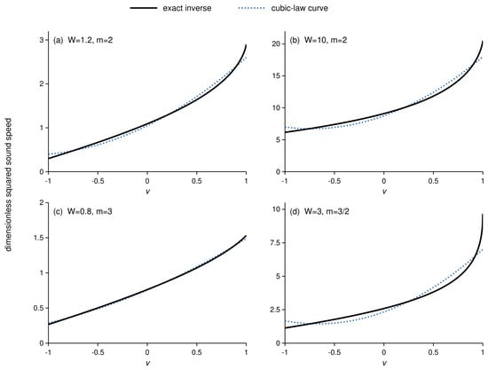
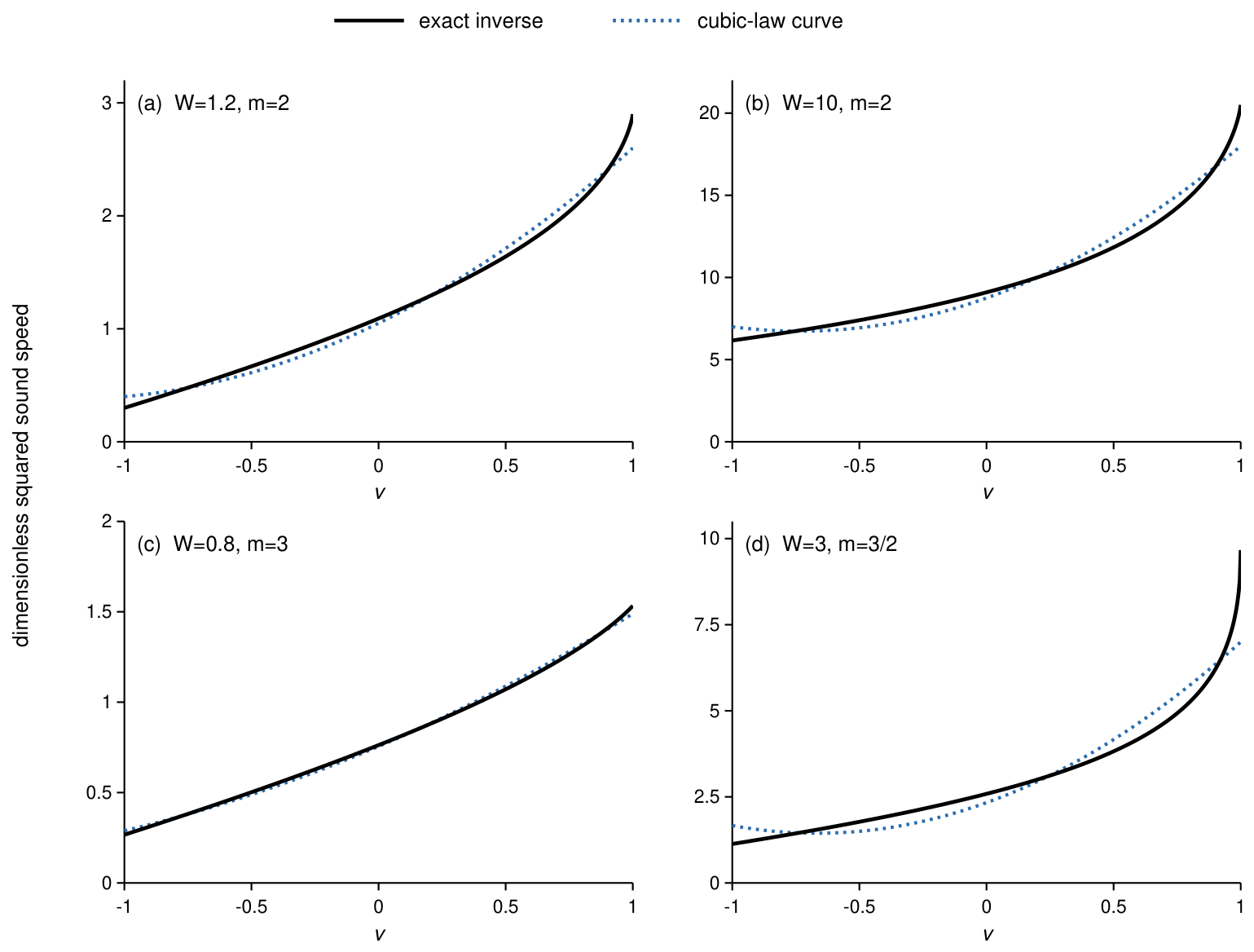
Since the exact and approximate results become asymptotically identical in the broad-shock limit, it is natural to examine how well the approximate construction reproduces the exact squared sound speed for finite values of m, including values outside the strict asymptotic regime. In Figure 3, we plot the exact and approximate dimensionless squared sound speeds $w_{W,m}\left(v\right)$ and $w_{W,m}^{\mathrm{cub}}\left(v\right)$ for several values of m and W. Each parameter pair used in this figure satisfies the physical admissibility conditions for both constructions.

Figure 3. Comparison of the exact dimensionless squared sound speed $w_{W,m}\left(v\right)$ obtained from Equation (55) (solid black line) and the dimensionless squared sound speed $w_{W,m}^{\mathrm{cub}}\left(v\right)$ associated with the cubic voltage–charge relation in Equation (76) (blue dotted line): (a) $W=1.2$, $m=2$; (b) $W=10$, $m=2$; (c) $W=0.8$, $m=3$; and (d) $W=3$, $m=3/2$.

6. Spectral Problem

In this section, we discard the assumptions of a monotonic profile and of a particular asymptotic behavior near the front edges, so the results can be applied both to shocks and to kinks. We next analyze the dispersion relation in the laboratory frame. The dispersion relation in the moving frame [18] is considered in Section 6.2. Stability and the kink–shock dichotomy are discussed in Section 6.3.

6.1. Spectral Problem in the Laboratory Frame

Equations (3) and (4) can be written as

$$\begin{array}{cc}\hfill {\mathit{\partial }}_{t}Q+\left({\displaystyle \frac{L}{R_L}}{\mathit{\partial }}_t+1\right){\mathit{\partial }}_{z}I& =0,\hfill \\ \hfill \left[R_C{\mathit{\partial }}_t+L{u}^2\left(Q(z,t)\right)\right]{\mathit{\partial }}_{z}Q+L{\mathit{\partial }}_{t}I& =0.\hfill \end{array}$$

(84)

We use a local frozen-background, or WKB-type, approximation appropriate to wavelengths short compared with the front width. Specifically, we neglect derivatives of the slowly varying coefficient $u_{\mathrm{fr}}^2=u^2\left(Q_{\mathrm{fr}}(z,t)\right)$ and treat it as locally constant. Its dependence on $(z,t)$ then enters only parametrically through its local value.

We consider small perturbations of the front solution

$$\begin{array}{cc}\hfill Q(z,t)& =Q_{\mathrm{fr}}(z,t)+ϵe^{\lambda t}\varphi \left(z\right),\left|ϵ\right|\ll 1,\hfill \\ \hfill I(z,t)& =I_{\mathrm{fr}}(z,t)+ϵe^{\lambda t}\psi \left(z\right).\hfill \end{array}$$

(85)

Substituting Equation (85) into Equation (84) and linearizing, we obtain the local eigenvalue problem

$$\begin{array}{cc}\hfill \lambda \varphi +\left({\displaystyle \frac{L}{R_L}}\lambda +1\right){\mathit{\partial }}_z\psi & =0,\hfill \\ \hfill \left(R_C\lambda +L{u}_{\mathrm{fr}}^2\right){\mathit{\partial }}_z\varphi +L\lambda \psi & =0.\hfill \end{array}$$

(86)

We seek normal-mode solutions of the form

$$\varphi \left(z\right)=\widehat{\varphi }{e}^{ikz},\psi \left(z\right)=\widehat{\psi }{e}^{ikz},k\in \mathbb{R},$$

(87)

where $\widehat{\varphi }$ and $\widehat{\psi }$ are constants. The resulting dispersion relation is

$$L\left(R_L+R_C{k}^2\right){\lambda }^2+\left(R_L{R}_C+L^2{u}_{\mathrm{fr}}^2\right)k^2\lambda +R_{L}L{u}_{\mathrm{fr}}^2{k}^2=0.$$

(88)

Hence, the two spectral branches are

$${\lambda }_{\pm }\left(k\right)={\displaystyle \frac{-\left(R_L{R}_C+L^2{u}_{\mathrm{fr}}^2\right)k^2\pm \sqrt{{\left(R_L{R}_C+L^2{u}_{\mathrm{fr}}^2\right)}^2{k}^4-4L^2{R}_L\left(R_L+R_C{k}^2\right)u_{\mathrm{fr}}^2{k}^2}}{2L\left(R_L+R_C{k}^2\right)}}.$$

(89)

6.2. Spectral Problem in the Moving Frame

We introduce the comoving coordinate

$$\xi =z-Ut.$$

(90)

In the coordinates $(\xi ,t)$, Equation (84) becomes

$$\begin{array}{cc}\hfill \mathcal{D}Q+{\mathcal{D}}_{\xi }\left({\displaystyle \frac{L}{R_L}}\mathcal{D}+1\right)I& =0,\hfill \\ \hfill \left[R_C\mathcal{D}+L{u}^2\left(Q(\xi ,t)\right)\right]{\mathcal{D}}_{\xi }Q+L\mathcal{D}I& =0,\hfill \end{array}$$

(91)

where

$$\begin{array}{cc}\hfill {\mathcal{D}}_{\xi }& \equiv {\left({\mathit{\partial }}_{\xi }\right)}_t={\left({\mathit{\partial }}_z\right)}_t,\hfill \\ \hfill {\mathcal{D}}_t& \equiv {\left({\mathit{\partial }}_t\right)}_{\xi }={\left({\mathit{\partial }}_t\right)}_z+U{\left({\mathit{\partial }}_z\right)}_t,\hfill \\ \hfill \mathcal{D}& \equiv {\left({\mathit{\partial }}_t\right)}_z={\mathcal{D}}_t-U{\mathcal{D}}_{\xi }.\hfill \end{array}$$

(92)

We consider a small perturbation of the front solution

$$\left\{\begin{array}{cc}Q(\xi ,t)\hfill & =Q_{\mathrm{fr}}\left(\xi \right)+ϵe^{\tilde{\lambda }t}\varphi \left(\xi \right),\hfill \\ I(\xi ,t)\hfill & =I_{\mathrm{fr}}\left(\xi \right)+ϵe^{\tilde{\lambda }t}\psi \left(\xi \right),\hfill \end{array}\right.\left|ϵ\right|\ll 1.$$

(93)

This ansatz should be compared with Equation (85). Substituting Equation (93) into Equation (91) and linearizing, we obtain a variable-coefficient eigenvalue problem [19]:

$$\begin{array}{c}\hfill U{\varphi }^{{\displaystyle \prime }}\left(\xi \right)+{\displaystyle \frac{d}{d\xi }}\left[{\displaystyle \frac{UL}{R_L}}{\psi }^{{\displaystyle \prime }}\left(\xi \right)-\psi \left(\xi \right)\right]=\tilde{\lambda }\left[\varphi \left(\xi \right)+{\displaystyle \frac{L}{R_L}}{\psi }^{{\displaystyle \prime }}\left(\xi \right)\right],\\ \hfill {\displaystyle \frac{d}{d\xi }}\left[U{R}_C{\varphi }^{{\displaystyle \prime }}\left(\xi \right)-L{u}_{\mathrm{fr}}^2\left(\xi \right)\varphi \left(\xi \right)\right]+UL{\psi }^{{\displaystyle \prime }}\left(\xi \right)=\tilde{\lambda }\left[R_C{\varphi }^{{\displaystyle \prime }}\left(\xi \right)+L\psi \left(\xi \right)\right].\end{array}$$

(94)

Here $u_{\mathrm{fr}}^2\left(\xi \right)=u^2\left(Q_{\mathrm{fr}}\left(\xi \right)\right)$. For the point spectrum, we seek localized eigenfunctions satisfying the boundary conditions

$$\left\{\begin{array}{cc}\varphi \left(\xi \right)\hfill & ⟶0,\hfill \\ \psi \left(\xi \right)\hfill & ⟶0,\hfill \end{array}\right.\xi ⟶\pm \infty .$$

(95)

Note that translational invariance implies the neutral eigenvalue $\tilde{\lambda }=0$, with eigenfunctions

$$\left\{\begin{array}{c}\varphi \left(\xi \right)=Q_{\mathrm{fr}}^{{\displaystyle \prime }}\left(\xi \right),\hfill \\ \psi \left(\xi \right)=I_{\mathrm{fr}}^{{\displaystyle \prime }}\left(\xi \right).\hfill \end{array}\right.$$

(96)

Indeed, a t-independent solution of Equation (91) satisfies the equations

$$\begin{array}{cc}\hfill U{Q}_{\mathrm{fr}}^{{\displaystyle \prime }}\left(\xi \right)+{\displaystyle \frac{d}{d\xi }}\left[{\displaystyle \frac{UL}{R_L}}{I}_{\mathrm{fr}}^{{\displaystyle \prime }}\left(\xi \right)-I_{\mathrm{fr}}\left(\xi \right)\right]& =0,\hfill \\ \hfill U{R}_C{Q}_{\mathrm{fr}}^{{\displaystyle ″}}\left(\xi \right)-L{u}_{\mathrm{fr}}^2\left(\xi \right)Q_{\mathrm{fr}}^{{\displaystyle \prime }}\left(\xi \right)+UL{I}_{\mathrm{fr}}^{{\displaystyle \prime }}\left(\xi \right)& =0.\hfill \end{array}$$

(97)

Differentiating Equation (97) with respect to $\xi$, we obtain

$$\begin{array}{cc}\hfill U{Q}_{\mathrm{fr}}^{{\displaystyle ″}}\left(\xi \right)+{\displaystyle \frac{d}{d\xi }}\left[{\displaystyle \frac{UL}{R_L}}{I}_{\mathrm{fr}}^{{\displaystyle ″}}\left(\xi \right)-I_{\mathrm{fr}}^{{\displaystyle \prime }}\left(\xi \right)\right]& =0,\hfill \\ \hfill {\displaystyle \frac{d}{d\xi }}\left[U{R}_C{Q}_{\mathrm{fr}}^{{\displaystyle ″}}\left(\xi \right)-L{u}_{\mathrm{fr}}^2\left(\xi \right)Q_{\mathrm{fr}}^{{\displaystyle \prime }}\left(\xi \right)\right]+UL{I}_{\mathrm{fr}}^{{\displaystyle ″}}\left(\xi \right)& =0.\hfill \end{array}$$

(98)

Equation (98) is Equation (94) evaluated at $\tilde{\lambda }=0$ with $(\varphi \left(\xi \right),\psi \left(\xi \right))=(Q_{\mathrm{fr}}^{{\displaystyle \prime }}\left(\xi \right),I_{\mathrm{fr}}^{{\displaystyle \prime }}\left(\xi \right))$, confirming the neutral translational mode. Spectral stability in the moving frame requires that, apart from the translational eigenvalue at $\tilde{\lambda }=0$, the spectrum contain no points with $\mathrm{Re}\tilde{\lambda }>0$.

In a local frozen-background approximation, using $\varphi \left(\xi \right)=\widehat{\varphi }{e}^{ik\xi }$ and $\psi \left(\xi \right)=\widehat{\psi }{e}^{ik\xi }$, with $k\in \mathbb{R}$, we recover Equations (88) and (89), as expected, with

$$\tilde{\lambda }=\lambda +iUk.$$

(99)

6.3. Stability and the Kink–Shock Dichotomy

For physically admissible states, $u_{\mathrm{fr}}^2>0$, and both spectral branches ${\tilde{\lambda }}_{\pm }$ (equivalently, ${\lambda }_{\pm }$) have negative real parts for $k\ne 0$. Thus, within the range of validity of the short-wavelength approximation, all nonzero real-wavenumber modes of the local frozen-coefficient problem are damped.

In either asymptotic state, where $Q_{\mathrm{fr}}=Q_i$, $u_{\mathrm{fr}}$ is constant. Hence Equations (88) and (89) are exact and valid for arbitrary real k, without invoking the short-wavelength approximation. We now consider long-wavelength perturbation modes in these states. Expanding Equation (89) for small k and retaining the leading term, we obtain

$${\tilde{\lambda }}_{i,\pm }\left(k\right)=i\left(U\pm u_i\right)k+O\left(k^2\right).$$

(100)

Focusing on the right-propagating branch makes the distinction between kinks and shocks transparent. In the case

$$u_1<U<u_2,$$

(101)

the front overtakes right-propagating long-wavelength disturbances in the state ahead of it, whereas such disturbances in the state behind it overtake the shock. By contrast, for

$$U>\max \{u_1,u_2\},$$

(102)

the front overtakes right-propagating disturbances in both asymptotic states and is therefore noncompressive. The mechanical analogy is therefore not essential for distinguishing kinks from shocks: the same classification follows directly from the long-wavelength characteristic structure of the original partial differential equations.

7. Conclusions

We considered a lossy transmission line with a nonlinear voltage–charge relation $V\left(Q\right)$ and derived an equation for a traveling front with the charge approaching constant asymptotic values on both sides of the front

$${\displaystyle \frac{d^{2}Q}{d{\theta }^2}}+\left[1+w\left(Q\right)\right]{\displaystyle \frac{dQ}{d\theta }}=W\left[Q-\overline{Q}\right]-C\left[V\left(Q\right)-\overline{V}\right],$$

(103)

where $\theta$ is the dimensionless time. Within the inverse-design approach, we prescribed the traveling-wave profile $v\left(\theta \right)$, where v is the dimensionless charge, and the dimensionless squared front speed W, and determined the dimensionless squared local sound speed w within the front, which was the central object of our analysis. We obtained

$$w_W\left(v\right)=-W{\Theta }^{{\displaystyle \prime }}\left(v\right){\int }_{-1}^v{\displaystyle \frac{ds}{\Theta \left(s\right)}}-S^{{\displaystyle \prime }}\left(v\right),$$

(104)

where $S\left(v\right)=dv/d\theta$ is the local slope of the scaled front profile $v\left(\theta \right)$, and $\Theta =-e^{-\theta }$ is the exponential variable. The squared sound speed, averaged uniformly over the charge interval spanned by the front, is equal to the squared front speed. The voltage–charge relation for the transmission line that supports the front was determined as

$$V_W\left(v\right)=V^{\mathrm{lin}}\left(v\right)-{\displaystyle \frac{\Delta V}{2}}\Theta \left(v\right)\left[{\int }_{-1}^v{\displaystyle \frac{ds}{\Theta \left(s\right)}}-{\displaystyle \frac{1}{W{\Theta }^{{\displaystyle \prime }}\left(v\right)}}\right].$$

(105)

We explicitly considered a hyperbolic-tangent front profile characterized by the dimensionless width parameter m. All physically admissible fronts of this form are shocks rather than kinks. The sound speed increases monotonically across the shock, from the state ahead of the front to the state behind it. Equations (104) and (105) in this case take the form

$$\begin{array}{cc}\hfill w_{W,m}\left(v\right)& =mW{(R+1)}^2{\int }_0^1{\displaystyle \frac{y^m}{{(1+Ry)}^2}}dy+{\displaystyle \frac{v}{m}},\hfill \end{array}$$

(106)

$$\begin{array}{cc}\hfill V_{W,m}\left(v\right)& =V^{\mathrm{lin}}\left(v\right)-\Delta V\left[R{\int }_0^1{\displaystyle \frac{y^m}{{(1+Ry)}^2}}dy+{\displaystyle \frac{1-v^2}{4mW}}\right],\hfill \end{array}$$

(107)

where $R={\displaystyle \frac{1+v}{1-v}}$.

We also treated a transmission line with a cubic voltage–charge relation and derived an approximate traveling-wave equation. The hyperbolic-tangent shock profile is an exact solution of this equation. In this formulation, after one shock parameter is prescribed, the remaining three are determined by that choice and by the coefficients of the voltage–charge relation. The results obtained within this approximate approach coincide with the broad-shock approximation of the exact inverse solution.

We examined stability of the front in terms of the original partial differential equations. The short-wavelength perturbation modes turned out to be damped.

The kink–shock distinction obtained from the mechanical analogy was independently confirmed through the long-wavelength characteristic analysis. The shock overtakes right-propagating long-wavelength disturbances in the state ahead of it, whereas such disturbances in the state behind it overtake the shock. By contrast, a kink overtakes right-propagating long-wavelength disturbances in both asymptotic states and is therefore noncompressive.

References

- Landauer, R. Shock Waves in Nonlinear Transmission Lines and Their Effect on Parametric Amplification. IBM J. Res. Dev. 1960, 4, 391–401. [Google Scholar] [CrossRef] [Scilit]
- Hirota, R.; Suzuki, K. Studies on Lattice Solitons by Using Electrical Networks. J. Phys. Soc. Jpn. 1970, 28, 1366–1367. [Google Scholar] [CrossRef] [Scilit]
- Kengne, E.; Malomed, B.A.; Chui, S.T.; Liu, W.M. Solitary Signals in Electrical Nonlinear Transmission Line. J. Math. Phys. 2007, 48, 013508. [Google Scholar] [CrossRef] [Scilit]
- Veldes, G.P.; Cuevas, J.; Kevrekidis, P.G.; Frantzeskakis, D.J. Coupled Backward- and Forward-Propagating Solitons in a Composite Right- and Left-Handed Transmission Line. Phys. Rev. E 2013, 88, 013203. [Google Scholar] [CrossRef] [Scilit] [PubMed]
- Powell, D.A.; Shadrivov, I.V.; Kivshar, Y.S. Multistability in Nonlinear Left-Handed Transmission Lines. Appl. Phys. Lett. 2008, 92, 264104. [Google Scholar] [CrossRef] [Scilit]
- English, L.Q.; Palmero, F.; Stormes, J.F.; Cuevas, J.; Carretero-González, R.; Kevrekidis, P.G. Nonlinear Localized Modes in Two-Dimensional Electrical Lattices. Phys. Rev. E 2013, 88, 022912. [Google Scholar] [CrossRef] [Scilit] [PubMed]
- Duran, H.; Cuevas-Maraver, J.; Kevrekidis, P.G.; Vainchtein, A. Moving Discrete Breathers in a β-FPU Lattice Revisited. Commun. Nonlinear Sci. Numer. Simul. 2022, 111, 106435. [Google Scholar] [CrossRef] [Scilit]
- Katayama, H.; Hatakenaka, N.; Matsuda, K.-I. Analogue Hawking Radiation in Nonlinear LC Transmission Lines. Universe 2021, 7, 334. [Google Scholar] [CrossRef] [Scilit]
- Bloom, F. Formation of Shock Discontinuities for a Class of Nonlinear Transmission Lines. Comput. Math. Appl. 1988, 15, 459–472. [Google Scholar] [CrossRef] [Scilit][Green Version]
- González, G.; Rosu, H.C.; Cornejo-Pérez, O.; Mancas, S.C. Factorization Conditions for Nonlinear Second-Order Differential Equations. In Nonlinear and Modern Mathematical Physics; Manukure, S., Ma, W.-X., Eds.; Springer International Publishing: Cham, Switzerland, 2024; pp. 81–99. [Google Scholar]
- Kudryashov, N.A. Exact Solutions and Integrability of the Duffing–Van der Pol Equation. Regul. Chaotic Dyn. 2018, 23, 471–479. [Google Scholar] [CrossRef] [Scilit]
- Kaliappan, P. An Exact Solution for Travelling Waves of ut = Duxx + u − uk. Phys. D. 1984, 11, 368–374. [Google Scholar] [CrossRef] [Scilit]
- Kogan, E. Shock Waves in Nonlinear Transmission Lines. Phys. Status Solidi B 2025, 262, 2400335. [Google Scholar] [CrossRef] [Scilit]
- Kogan, E. Nonlinear Transmission Line: Shock Waves and the Simple Wave Approximation. Mathematics 2025, 13, 3215. [Google Scholar] [CrossRef] [Scilit]
- Whitham, G.B. Linear and Nonlinear Waves; John Wiley & Sons: New York, NY, USA, 1999. [Google Scholar]
- Temme, N.M. Special Functions: An Introduction to the Classical Functions of Mathematical Physics; Wiley: New York, NY, USA, 1996. [Google Scholar]
- Wong, R. Asymptotic Approximations of Integrals; Academic Press: New York, NY, USA, 1989. [Google Scholar]
- Lifshitz, E.M.; Pitaevskii, L.P. Physical Kinetics; Course of Theoretical Physics; Chapter VI; Pergamon Press: Oxford, UK, 1981; Volume 10. [Google Scholar]
- Reed, M.; Simon, B. Methods of Modern Mathematical Physics, Vol. IV: Analysis of Operators; Academic Press: New York, NY, USA, 1978. [Google Scholar]
Disclaimer/Publisher’s Note: The statements, opinions and data contained in all publications are solely those of the individual author(s) and contributor(s) and not of MDPI and/or the editor(s). MDPI and/or the editor(s) disclaim responsibility for any injury to people or property resulting from any ideas, methods, instructions or products referred to in the content. |
© 2026 by the author. Licensee MDPI, Basel, Switzerland. This article is an open access article distributed under the terms and conditions of the Creative Commons Attribution (CC BY) license.