A Bisection Eigenvalue Algorithm for Symmetric Quasiseparable Matrices

Abstract

In this paper we design a fast bisection algorithm for computing a prescribed eigenvalue of a symmetric quasiseparable matrix represented by its Cholesky-like factorization $A_0=L_0{\Omega }_0{L}_0^T$, where $L_0$ is a lower triangular quasiseparable matrix and ${\Omega }_0$ is a signature matrix. The workhorse of the algorithm is an efficient linear-time scheme for updating the factorization under shifting. Numerical experiments illustrate the effectiveness and the robustness of the proposed method.

1. Introduction

Symmetric eigenvalue problems arise, directly or indirectly, in many areas of science and engineering. Bisection is one of the standard tools for computing all the eigenvalues of a matrix, or only a selected few, and it remains attractive because it lends itself to parallel and concurrent implementation. We do not deal here with the computation of eigenvectors; this can be carried out by any preferred technique, for instance inverse iteration with shift. There is currently a growing interest in the design of efficient eigenvalue algorithms for quasiseparable and, more generally, rank-structured matrices (see, for instance, [1,2]). Such matrices arise naturally in applications, for example, in structural mechanics and fluid dynamics, through the spatial discretization of partial differential equations and integral equations. They are often very large, but they are structured, in the sense that their off-diagonal blocks have low rank relative to the size of the matrix. The class of quasiseparable matrices contains the banded matrices as a subclass.

Fast adaptations of the bisection method for the eigenvalue computation of Hermitian quasiseparable matrices have been proposed in [3,4]. These methods rely on efficient schemes for evaluating the Sturm sequence of polynomials associated with a Hermitian quasiseparable matrix by means of short-term recurrence relations. For quasiseparable matrices of order one, such a scheme was first presented in [5]. Polynomials and recurrences lead to elegant and theoretically fast algorithms, but they also cause serious numerical stability problems in floating-point arithmetic. To mitigate these issues, scaling procedures are introduced in [3,4] in order to keep the growth of the intermediate coefficients under control. Even so, these techniques may lose accuracy on matrices with clustered eigenvalues or with entries of widely varying magnitude.

Symmetric $LU$ factorizations provide an alternative to Sturm sequences for counting the positive and the negative eigenvalues of a symmetric matrix A [6]. Let $A_{\alpha }=A-\alpha I=L_{\alpha }{\Omega }_{\alpha }{L}_{\alpha }^T$, where $\alpha \in \mathbb{R}$, $L_{\alpha }$ is lower triangular and ${\Omega }_{\alpha }$ is a signature matrix, be a Cholesky-like factorization of the shifted matrix $A_{\alpha }$. If $\alpha$ does not belong to the spectrum of A, then Sylvester’s law of inertia (Theorem 4.5.8 in [7]) shows that the number of eigenvalues of A smaller than $\alpha$ equals the number of negative diagonal entries of ${\Omega }_{\alpha }$.

In this paper we present a fast bisection-type method for the eigenvalue computation of Hermitian quasiseparable matrices of arbitrary order. The method is based on an efficient algorithm for updating the triangular factorization of $A_0$ under shifting, that is, for carrying out the transformations $L_0\to L_{\alpha }$ and ${\Omega }_0\to {\Omega }_{\alpha }$. If all the eigenvalues of $A=A_0$ lie in the interval $(a,b)$, then the initial factorization of $A_0$ can be obtained by updating the Cholesky factorization of the definite matrix $A_a$ or $A_b$. Efficient linear-complexity algorithms for computing the Cholesky factorization of a definite quasiseparable matrix are available in the literature [2].

The updating procedure makes use of (generalized) orthogonal and hyperbolic transformations [8]. Non-unitary variants of standard algorithms for computing all the eigenvalues of structured matrices have already appeared in the literature (see, for instance, [9,10]). Because the transformations are not unitary, stability is not guaranteed, and such algorithms can occasionally terminate prematurely or lose accuracy through the growth of the coefficients. These occurrences are nevertheless very rare, they can be monitored dynamically, and they can be dealt with by restarting or by shifting.

Whenever our factorization scheme runs to completion, it returns the updated triangular factor $L_{\alpha }$, represented via generators, together with the updated signature matrix ${\Omega }_{\alpha }$. Computing the initial Cholesky factorization of a symmetric quasiseparable matrix of size n and quasiseparability order $\kappa$ given by its generators costs $O\left(n{\kappa }^3\right)$ flops [11], and it returns the generators of the lower and upper triangular factors with quasiseparability order at most $\kappa$. Starting from these generators, the updating procedure computes a representation of $L_{\alpha }$ in the out-of-band quasiseparable form of [12], in which most of the generators of $L_{\alpha }$ coincide with those of $L_0$. The approach therefore saves a substantial amount of work in terms of the leading constants. Moreover, if $L_0$ is semiseparable of order $\kappa$, then the modified factorization can be computed in $O\left(n{\kappa }^2\right)$ flops, so that our bisection method needs $O(n{\kappa }^3+\ell n{\kappa }^2)$ flops to perform ℓ bisection steps. Numerical results are reported to confirm the effectiveness and the robustness of the resulting algorithm.

The paper is organized as follows. In Section 2 we fix the notation and recall some preliminary results, whereas in Section 3 we review the updating procedure for symmetric triangular factorizations. Section 4 develops our bisection eigenvalue algorithm for symmetric quasiseparable matrices of arbitrary order. Section 5 is devoted to the numerical experiments, which confirm the efficiency and the robustness of the proposed method. Conclusions and directions for future work are given in Section 6.

2. Preliminaries

This paper is concerned with the eigenvalue computation of rank-structured matrices specified in terms of generators. We first recall the following definition [11].

Definition 1. 

A matrix $A=\left(a_{i,j}\right)\in {\mathbb{R}}^{n\times n}$ is quasiseparable of order κ if there exist lower generators ${\mathit{p}}_i\in {\mathbb{R}}^{\kappa }$, $2\le i\le n$, ${\mathit{q}}_j\in {\mathbb{R}}^{\kappa }$, $1\le j\le n-1$, $A_{\ell }\in {\mathbb{R}}^{\kappa \times \kappa }$, $2\le \ell \le n-1$ and upper generators ${\mathit{g}}_i\in {\mathbb{R}}^{\kappa }$, $1\le i\le n-1$, ${\mathit{h}}_j\in {\mathbb{R}}^{\kappa }$, $2\le j\le n$, $B_{\ell }\in {\mathbb{R}}^{\kappa \times \kappa }$, $2\le \ell \le n-1$, such that

$$a_{i,j}=\left\{\begin{array}{c}{\mathit{p}}_i^T\overleftarrow{A_{i,j}}{\mathit{q}}_j\mathrm{if}i>j,\hfill \\ {\mathit{g}}_i^T\overrightarrow{B_{i,j}}{\mathit{h}}_j\mathrm{if}i<j,\hfill \end{array}\right.$$

where we denote

$$\overleftarrow{A_{i,j}}=\left\{\begin{array}{c}{A}_{i-1}\cdots A_{j+1}\mathrm{if}i>j+1,\hfill \\ I_{\kappa }\mathrm{if}i=j+1,\hfill \end{array}\right.\overrightarrow{B_{i,j}}=\left\{\begin{array}{c}{B}_{i+1}\cdots B_{j-1}\mathrm{if}j>i+1,\hfill \\ I_{\kappa }\mathrm{if}j=i+1.\hfill \end{array}\right.$$

When $A_i=B_i=I_{\kappa }$, the identity matrix of order κ, $2\le i\le n-1$, the matrix A is called semiseparable of order κ.

The triangular factors of a quasiseparable matrix inherit the rank structure of the matrix itself [2].

Definition 2. 

Let $A\in {\mathbb{R}}^{n\times n}$ be a symmetric possibly indefinite matrix. A Cholesky-like factorization of A has the form $A=L\Omega L^T$ where $L\in {\mathbb{R}}^{n\times n}$ is lower triangular and $\Omega =diag\left[\pm 1\right]$ is some diagonal signature matrix.

A strongly nonsingular symmetric matrix admits an essentially unique Cholesky-like factorization. If A is quasiseparable of order $\kappa$ and admits a Cholesky-like factorization $A=L\Omega L^T$ with L invertible, then L is quasiseparable of order at most $\kappa$. In addition, by Sylvester’s law of inertia (see Theorem 4.5.8 in [7]), A and $\Omega$ have the same numbers of positive, negative and zero eigenvalues.

In this paper we consider the problem of computing a modified Cholesky-like factorization of a quasiseparable matrix under shifting.

Definition 3. 

Given the Cholesky-like factorization of the symmetric matrix $A\in {\mathbb{R}}^{n\times n}$, that is, $A=A_0=L_0{\Omega }_0{L}_0^T$ where $L_0\in {\mathbb{R}}^{n\times n}$ is lower triangular and ${\Omega }_0$ is some diagonal signature matrix, the modified Cholesky-like factorization problem consists of computing a Cholesky-like factorization of $A_{\alpha }=A_0+\alpha I_n=L_{\alpha }{\Omega }_{\alpha }{L}_{\alpha }^T$.

Efficient numerical algorithms for solving the modified Cholesky-like factorization problem for matrices of low displacement rank, based on generalized unitary and hyperbolic transformations, are already available (see [8] and the references therein). The following definition generalizes the notion of a unitary matrix to vector spaces equipped with an indefinite scalar product [13].

Definition 4. 

For a given diagonal signature matrix $D=diag[\pm 1]\in {\mathbb{R}}^{n\times n}$ a matrix $Q\in {\mathbb{C}}^{n\times n}$ is called D-orthogonal if $Q^{T}DQ=D$.

A vector $\mathit{x}\in {\mathbb{R}}^n$ can be reduced to a scalar multiple of the last column of $I_n$ by a D-orthogonal matrix Q, annihilating one entry of x at a time in a process akin to the use of orthogonal Givens rotations. We may therefore restrict ourselves to the case $n=2$. For stability reasons it is also important to avoid the growth of the intermediate entries.  If $D=\pm I_2$ and $\mathit{x}={[x_1,x_2]}^T$ satisfies ${\mathit{x}}^T\mathit{x}\ne 0$ with $|x_1|\ge |x_2|$, then the Givens plane rotation matrix

$${\displaystyle \mathcal{G}=giv(x_1,x_2):=\frac{1}{\sqrt{1+{\rho }^2}}\left[\begin{array}{cc}-\rho & 1\\ 1& \rho \end{array}\right],\rho =\frac{x_2}{x_1},}$$

(1)

is such that   

$$\mathcal{G}\left[\begin{array}{c}{x}_1\\ x_2\end{array}\right]=\left[\begin{array}{c}0\\ y_1\end{array}\right],y_1={\displaystyle \frac{|x_1|}{x_1}}{\Vert x\Vert }_2,{\mathcal{G}}^T{I}_2\mathcal{G}=I_2.$$

If $D=\pm diag[1,-1]$ and ${\mathit{x}}^{T}D\mathit{x}\ne 0$ with $|x_1| > |x_2|$, then the hyperbolic rotation matrix $\mathcal{H}$

$${\displaystyle \mathcal{H}=hypf(x_1,x_2):=\frac{1}{\sqrt{1-{\rho }^2}}\left[\begin{array}{cc}-\rho & 1\\ 1& -\rho \end{array}\right],\rho =\frac{x_2}{x_1},}$$

(2)

maps x as required

$$\mathcal{H}\left[\begin{array}{c}{x}_1\\ x_2\end{array}\right]=\left[\begin{array}{c}0\\ y_1\end{array}\right],y_1={\displaystyle \frac{|x_1|}{x_1}}\sqrt{|{\mathit{x}}^{T}D\mathit{x}|},$$

and, moreover, it satisfies   

$${\mathcal{H}}^{T}D\mathcal{H}=-D={\mathcal{J}}_{2}D{\mathcal{J}}_2,$$

where   

$${\mathcal{J}}_2=\left[\begin{array}{cc}0& 1\\ 1& 0\end{array}\right].$$

Therefore, $H{\mathcal{J}}_2$ is D-orthogonal.

Givens and hyperbolic plane rotation matrices are extended to the complementary case $|x_1| < |x_2|$ by setting

$$giv(x_1,x_2)\leftarrow giv(x_2,x_1){\mathcal{J}}_2,hypf(x_1,x_2)\leftarrow hypf(x_2,x_1){\mathcal{J}}_2.$$

If $|x_1| = |x_2| \ne 0$, then the hyperbolic transformation $hypf(x_1,x_2)$ is not defined. If $\mathcal{U}\in \{\mathcal{G},\mathcal{G}{\mathcal{J}}_2,\mathcal{H}{\mathcal{J}}_2\}$, then $\mathcal{U}D{\mathcal{U}}^T = D_1 = D$, whereas for $\mathcal{U} = \mathcal{H}$ we find $\mathcal{U}D{\mathcal{U}}^T=D_1={\mathcal{J}}_{2}D{\mathcal{J}}_2$. We denote by $[\mathit{y},D_1,\mathcal{U}]=\mathrm{ZEROING}(\mathit{x},D)$ the procedure that, given as input $\mathit{x}\in {\mathbb{R}}^2$ and a $2\times 2$ signature matrix D, first determines $\mathcal{U}$ and then applies it to x and to D in order to compute $\mathcal{U}\mathit{x}=\mathit{y}={\left[0,y_1\right]}^T$ and $D_1$. We set $[\mathbf{0},D,I_2]=\mathrm{ZEROING}(\mathbf{0},D)$. A sequence of generalized plane rotations can then be used to annihilate the entries of a vector one after the other.

Remark 1. 

Some clarifications about the applicability of Procedure ELIMINATE stated in Algorithm 1 are in order. An annihilation scheme based on generalized plane rotations applied in a prescribed order can clearly break down prematurely. The order used here is dictated by our application to the modified Cholesky-like factorization problem for quasiseparable matrices. As with hyperbolic rotations, hyperbolic and unified Householder reflections [8,14] can be introduced as generalizations of the classical orthogonal Householder elementary matrices. If ${\mathit{v}}^T\Omega \mathit{v}\ne 0$, then a generalized Householder matrix Q can be determined so that $Q\mathit{v}=\theta {\mathit{e}}_n$ and $Q^T\Omega Q={\Omega }_1$. Generalizations of the schemes proposed here that use generalized Householder matrices will be treated elsewhere.

Algorithm 1 Procedure ELIMINATE. Given a vector $\mathit{v}\in {\mathbb{R}}^n$ and a signature matrix $\Omega \in {\mathbb{R}}^{n\times n}$, this algorithm attempts to compute a sequence of generalized plane rotations ${\mathcal{U}}_1,\dots ,{\mathcal{U}}_{n-1}$ such that the cumulative product $Q={\mathcal{U}}_{n-1}\cdots {\mathcal{U}}_1$ satisfies $Q\mathit{v}=\theta {\mathit{e}}_n$ and $Q^T\Omega Q={\Omega }_1$, with ${\Omega }_1$ a suitable signature matrix. A Boolean flag is also returned, indicating whether the zeroing scheme has run to completion.

1: $success=true$; 2: for $j=1:n-1$ do; 3:     $\mathit{x}=\mathit{v}\left(\right[j,n\left]\right)$; $D=\Omega \left(\right[j,n],[j,n\left]\right)$; 4:     if ${\mathit{x}}^{T}D\mathit{x}\ne 0\vee \mathit{x}==\mathbf{0}$  then 5:         $[\mathit{v}\left([j,n]\right),\Omega ([j,n],[j,n]),{\mathcal{U}}_j]=\mathrm{ZEROING}(\mathit{v}\left([j,n]\right),D)$; 6:     else 7:         $success=false$; 8:         break; 9:     end if 10: end for 11: ${\Omega }_1=\Omega$, $\theta ={\mathit{v}}_n$.

3. An Updating Procedure for Symmetric Triangular Factorizations of Shifted Quasiseparable Matrices

In this section we present the algorithm developed in [15] for the efficient solution of the modified Cholesky-like factorization problem for symmetric quasiseparable matrices. This algorithm is the fundamental building block of the bisection method proposed here.

Let $A\in {\mathbb{R}}^{n\times n}$ be a symmetric, possibly indefinite, matrix and let $A=A_0=L_0{\Omega }_0{L}_0^T$ be its Cholesky-like triangular factorization, where $L_0$ is lower triangular and ${\Omega }_0$ is a signature matrix. We are interested in computing a Cholesky-like triangular factorization of the shifted matrix $A_{\alpha }=A+\alpha I_n=L_{\alpha }{\Omega }_{\alpha }{L}_{\alpha }^T$, $\alpha \in \mathbb{R}$. Following [8], we first describe the general strategy for the modified Cholesky problem and then show how to adapt it to quasiseparable matrices.

Let us start by observing that

$$A_{\alpha }=\left[\begin{array}{ccc}{L}_0& |& \sqrt{\left|\alpha \right|}\end{array}\right]\left[\begin{array}{cc}{\Omega }_0& \\ & \pm I\end{array}\right]\left[\begin{array}{c}{L}_0^T\\ \sqrt{\left|\alpha \right|}\end{array}\right]=\left[\begin{array}{ccc}{L}_0& |& \sqrt{\left|\alpha \right|}\end{array}\right]{\widehat{\Omega }}_0\left[\begin{array}{c}{L}_0^T\\ \sqrt{\left|\alpha \right|}\end{array}\right].$$

The matrix ${\widehat{\Omega }}_0$ is again a signature matrix, which makes it possible to devise an orthogonalization-like process that annihilates the entries of $L_0$ and $L_0^T$ incrementally. Specifically, define $R_0={\left[\begin{array}{ccc}{L}_0& |& \sqrt{\left|\alpha \right|}\end{array}\right]}^T$ such that

$$A_{\alpha }=A+\alpha I_n=R_0^T{\widehat{\Omega }}_0{R}_0.$$

(3)

When A is quasiseparable, a fast algorithm for computing the updated triangular factorization of $A_{\alpha }=A+\alpha I$ can be obtained by interlacing band reduction stages with a bulge chasing scheme. The reduction to banded form is accomplished by a process similar to the modification of the Dewilde-van der Veen method described in [16]. Some of the computations in the band reduction stages can be performed offline and stored, which saves work in the updating procedure.

To convey the idea, and for the sake of simplicity, we begin with quasiseparable matrices of quasiseparability rank $\kappa =1$. Let $R=R_0$ be as in (3), where $L_0^T$ is quasiseparable with upper quasiseparability rank $\kappa =1$. We first apply a plane rotation in the plane of the coordinates $(1,2)$ in order to zero some entries in the first row of $L_0^T$. Because of the rank structure, this reduces R to the form

$$R=\left[\frac{\begin{array}{cccc}x& x& 0& 0\\ x& x& x& x\\ & & x& x\\ & & & x\end{array}}{\begin{array}{cccc}x& & & \\ & x& & \\ & & x& \\ & & & x\end{array}}\right].$$

The annihilation in the first row generates a bulge in the top-left corner of the matrix R. We then nullify the first column of this bulge by applying two plane rotations in the planes $(1,n+1)$ and $(2,n+1)$ to annihilate $R(1,1)$ and $R(2,1)$, respectively. Notice that the newly generated row in the bottom part of R is a linear combination of the first two rows and therefore it exhibits an out-of-band quasiseparable structure. Moreover, after this zeroing, the second row of R also has an out-of-band quasiseparable representation. At the end of the first step the matrix R has the following profile:

$$R=\left[\frac{\begin{array}{cccc}0& x& 0& 0\\ 0& x& x& x\\ & & x& x\\ & & & x\end{array}}{\begin{array}{cccc}x& x& x& x\\ & x& & \\ & & x& \\ & & & x\end{array}}\right].$$

The out-of-band quasiseparable structure is preserved throughout the zeroing process, so that, if the algorithm terminates successfully, at the very end the matrix R has the form

$$R=\left[\frac{\begin{array}{cccc}0& 0& 0& 0\\ 0& 0& 0& 0\\ 0& 0& 0& 0\\ 0& 0& 0& 0\end{array}}{\begin{array}{cccc}x& x& x& x\\ & x& x& x\\ & & x& x\\ & & & x\end{array}}\right],$$

where the triangular factor in the lower part of R has an out-of-band quasiseparable parametrization with quasiseparability rank at most 1.

The generalization of this approach to quasiseparable matrices of arbitrary order is considered below in more detail. Let $L_0^T\in {\mathbb{R}}^{n\times n}$ be an upper quasiseparable matrix of order $\kappa$ with upper generators ${\mathit{g}}_i\in {\mathbb{R}}^{\kappa }$, $1\le i\le n-1$, ${\mathit{h}}_j\in {\mathbb{R}}^{\kappa }$, $2\le j\le n$, $B_{\ell }\in {\mathbb{R}}^{\kappa \times \kappa }$, $2\le \ell \le n-1$. Set $R_0={\left[\begin{array}{ccc}{L}_0& |& \sqrt{\left|\alpha \right|}\end{array}\right]}^T$ and ${\Omega }_0$ such that $A=L_0{\Omega }_0{L}_0^T$. Recall that

$$A_{\alpha }=A+\alpha I_n=R_0^T{\widehat{\Omega }}_0{R}_0,{\widehat{\Omega }}_0=diag[{\Omega }_0,\pm I].$$

The updating of $L_0$ and ${\Omega }_0$ to $L_{\alpha }$ and ${\Omega }_{\alpha }$ proceeds in $n-1$ steps:

$$R_0\to R_1\to \dots \to R_{n-1}={\left[\begin{array}{ccc}0& |& {\widehat{S}}_{n-1}\end{array}\right]}^T,{\widehat{\Omega }}_0\to {\widehat{\Omega }}_1\to \dots \to {\widehat{\Omega }}_{n-1},$$

where ${{\widehat{S}}_{n-1}}^T$ is upper triangular, the matrices ${\widehat{\Omega }}_i$ are signature matrices and $R_0^T{\widehat{\Omega }}_0{R}_0=R_i^T{\widehat{\Omega }}_i{R}_i$ for $1\le i\le n-1$. The algorithm makes repeated calls to Procedure ELIMINATE, which is always assumed to terminate successfully. The first and the last $\kappa$ steps of the algorithm are special, because of boundary constraints and initializations, whereas the ℓ-th step, $\kappa +1\le \ell \le n-\kappa -1$, is generic. For the sake of illustration, we describe the initial step and a generic step below.

At the first step we consider the matrices

$$G_1=\left[\begin{array}{c}{\widehat{X}}_1{B}_{\kappa +1}\\ {\mathit{g}}_{\kappa +1}^T\end{array}\right]\in {\mathbb{R}}^{(\kappa +1)\times \kappa },{\widehat{X}}_1=\left[\begin{array}{c}{\mathit{g}}_1^T{B}_2\cdots B_{\kappa }\\ ⋮\\ {\mathit{g}}_{\kappa }^T\end{array}\right].$$

Then, by means of Procedure ELIMINATE we find a generalized QL factorization of $G_1$ of the form   

$$H_1{G}_1=\left[\begin{array}{c}{\mathbf{0}}^T\\ X_1\end{array}\right],X_1\in {\mathbb{R}}^{\kappa \times \kappa }\mathrm{lower}\mathrm{triangular},$$

with   

$$H_1{\widehat{\Omega }}_0(1:\kappa +1,1:\kappa +1)H_1^T={\Omega }_{1/2},$$

for a suitable diagonal signature matrix ${\Omega }_{1/2}$. The computation of $X_1$, $G_1$, $H_1$ and ${\widehat{X}}_1$ does not depend on the shift $\alpha$ and can therefore be carried out offline and stored. It follows that

$$R_0^T{\widehat{\Omega }}_0{R}_0=R_{1/2}^T{\widehat{\Omega }}_{1/2}{R}_{1/2},$$

with   

$${\widehat{\Omega }}_{1/2}=diag[{\Omega }_{1/2},{\widehat{\Omega }}_0(\kappa +2:n,\kappa +2:n)],$$

and   

$$R_{1/2}={\left[\begin{array}{ccc}{\widehat{L}}_{1/2}& |& \sqrt{\left|\alpha \right|}\end{array}\right]}^T,$$

where ${\widehat{L}}_{1/2}^T$ is generated from ${L_0}^T$ by modifying its first $\kappa +1$ rows so that

$${\widehat{L}}_{1/2}^T(1:\kappa +1,:)=H_1{R}_0(1:\kappa +1,:),$$

and   

$${\widehat{L}}_{1/2}^T(1:\kappa +1,:)=\left[\begin{array}{ccc}{F}_{1/2}& |& \frac{\begin{array}{c}{\mathbf{0}}^T\end{array}}{\begin{array}{c}\begin{array}{ccc}{X}_1{\mathit{h}}_{\kappa +2}& X_1{B}_{\kappa +2}{\mathit{h}}_{\kappa +3}& \dots \end{array}\end{array}}\end{array}\right].$$

The matrix $F_{1/2}\in {\mathbb{R}}^{(\kappa +1)\times (\kappa +1)}$ contains the bulge. Depending on the signatures involved, we now apply Givens or hyperbolic plane rotations in the planes of the coordinates $(1,n+1)$, $(2,n+1),\dots ,(\kappa +1,n+1)$ in order to annihilate the first column of $F_{1/2}$. Notice that $M=R_{1/2}([1:\kappa +1,n+1],:)$ is such that

$$M=\left[\begin{array}{ccc}\begin{array}{cc}{F}_{1/2}& \\ \sqrt{\left|\alpha \right|}& {\mathbf{0}}^T\end{array}& |& \frac{\begin{array}{c}{\mathbf{0}}^T\end{array}}{\begin{array}{c}\left[\begin{array}{c}{X}_1\\ {\mathbf{0}}^T\end{array}\right]\left[\begin{array}{ccc}{\mathit{h}}_{\kappa +2}& B_{\kappa +2}{\mathit{h}}_{\kappa +3}& \dots \end{array}\right]\end{array}}\end{array}\right].$$

The application of Procedure ELIMINATE to the first column of $R_{1/2}([1:\kappa +1,n+1],:)$ converts $R_{1/2}$ into $R_1$ with $M=R_1([1:\kappa +1,n+1],:)$ given by

$$M=\left[\begin{array}{ccc}\begin{array}{c}\begin{array}{cc}\mathbf{0}& F_1\end{array}\\ \\ {\mathit{s}}_1^T\end{array}& |& \frac{\begin{array}{c}{\mathbf{0}}^T\end{array}}{\begin{array}{c}\\ \left[\begin{array}{c}{\widehat{X}}_2\\ {\mathit{z}}_1^T\end{array}\right]\left[\begin{array}{ccc}{\mathit{h}}_{\kappa +2}& B_{\kappa +2}{\mathit{h}}_{\kappa +3}& \dots \end{array}\right]\end{array}}\end{array}\right],$$

where ${\widehat{X}}_2\in {\mathbb{R}}^{\kappa \times \kappa }$ is lower triangular. At the end of the first step we therefore find $R_1$ and a diagonal signature matrix ${\widehat{\Omega }}_1$ such that

$$R_1={\left[\begin{array}{ccc}{\widehat{L}}_1& |& {\widehat{S}}_1\end{array}\right]}^T,$$

with

$$\begin{array}{cc}\hfill {\widehat{L}}_1^T(1:\kappa +1,:)& =\left[\begin{array}{ccc}\begin{array}{ccc}\mathbf{0}& |& F_1\end{array}& |& \frac{\begin{array}{c}{\mathbf{0}}^T\end{array}}{\begin{array}{c}\\ \begin{array}{ccc}{\widehat{X}}_2{\mathit{h}}_{\kappa +2}& {\widehat{X}}_2{B}_{\kappa +2}{\mathit{h}}_{\kappa +3}& \dots \end{array}\end{array}}\end{array}\right],\hfill \\ \hfill {\widehat{S}}_1^T(1,:)& =\left[{\mathit{s}}_1^T,{\mathit{z}}_1^T{\mathit{h}}_{\kappa +2},{\mathit{z}}_1^T{B}_{\kappa +2}{\mathit{h}}_{\kappa +3},\dots ,{\mathit{z}}_1^T{B}_{\kappa +2}\dots B_{n-1}{\mathit{h}}_n\right],\hfill \\ \hfill {\widehat{S}}_1^T(\ell ,:)& =\sqrt{\left|\alpha \right|}{\mathit{e}}_{\ell }^T,2\le \ell \le n,\hfill \end{array}$$

and   

$$R_0^T{\widehat{\Omega }}_0{R}_0=R_1^T{\widehat{\Omega }}_1{R}_1.$$

At the second step the reduction is continued by first factoring the matrix

$$G_2=\left[\begin{array}{c}{\widehat{X}}_2{B}_{\kappa +2}\\ {\mathit{g}}_{\kappa +2}^T\end{array}\right]$$

as   

$$H_2{G}_2=\left[\begin{array}{c}{\mathbf{0}}^T\\ X_2\end{array}\right],X_2\in {\mathbb{R}}^{\kappa \times \kappa }\mathrm{lower}\mathrm{triangular}.$$

We then annihilate the first column of the bulge matrix $F_{3/2}$, which is determined so that

$$\begin{array}{cc}\hfill {\widehat{L}}_{3/2}^T(1:\kappa +2,2:n)& =\left[\begin{array}{ccc}{F}_{3/2}& |& \frac{\begin{array}{c}{\mathbf{0}}^T\\ {\mathbf{0}}^T\end{array}}{\begin{array}{c}\\ \begin{array}{ccc}{X}_2{\mathit{h}}_{\kappa +3}& X_2{B}_{\kappa +3}{\mathit{h}}_{\kappa +4}& \dots \end{array}\end{array}}\end{array}\right]\hfill \\ \hfill L_{3/2}^T& =(1\oplus H_2\oplus I_{n-\kappa -2})L_1^T.\hfill \end{array}$$

Here and hereafter ⊕ denotes the direct sum of matrices. Note that $F_{3/2}\in {\mathbb{R}}^{(\kappa +2)\times (\kappa +1)}$ has a zero entry in position $(1,\kappa +1)$. During the first $\kappa +1$ steps the matrix $F_{\ell -1/2}$ keeps growing by one row at a time, with zero entries entering from the right. After that, its first row becomes zero and can be discarded, so that the matrix moves down along the main diagonal with the constant size $(2\kappa +1)\times (\kappa +1)$.

At the generic step ℓ the zeroing scheme first computes the generalized QL decomposition of $G_{\ell }=\left[\begin{array}{c}{\widehat{X}}_{\ell }{B}_{\kappa +\ell }\\ {\mathit{g}}_{\kappa +\ell }^T\end{array}\right]$ as $H_{\ell }{G}_{\ell }=\left[\begin{array}{c}{\mathit{0}}^T\\ X_{\ell }\end{array}\right]$, with $X_{\ell }\in {\mathbb{R}}^{\kappa \times \kappa }$, and ${\widehat{H}}_{\ell }{\widehat{\Omega }}_{\ell -1}{\widehat{H}}_{\ell }^T={\widehat{\Omega }}_{\ell -1/2}$, ${\widehat{H}}_{\ell }=I_{\ell -1}\oplus H_{\ell }\oplus I_{2n-\ell -\kappa }$. It then computes $R_{\ell -1/2}={\widehat{H}}_{\ell }{R}_{\ell -1}$ and acts on the submatrix $M=R_{\ell -1/2}([\ell -\kappa :\ell +\kappa ,n+\ell ],:)$ given by

$$M=\left[\begin{array}{ccc}\begin{array}{cc}{F}_{\ell -1/2}& \\ \sqrt{\left|\alpha \right|}& {\mathbf{0}}^T\end{array}& |& \frac{\begin{array}{c}{0}_{\kappa +1,n-\kappa -\ell +1}\end{array}}{\begin{array}{c}\\ \left[\begin{array}{c}{X}_{\ell }\\ {\mathbf{0}}^T\end{array}\right]\left[\begin{array}{ccc}{\mathit{h}}_{\kappa +\ell +1}& B_{\kappa +\ell +1}{\mathit{h}}_{\kappa +\ell +2}& \dots \end{array}\right]\end{array}}\end{array}\right],$$

where $X_{\ell }\in {\mathbb{R}}^{\kappa \times \kappa }$ is lower triangular and, moreover, $F_{\ell -1/2}\in {\mathbb{R}}^{(2\kappa +1)\times (\kappa +1)}$ is a trapezoidal matrix such that   

$$F_{\ell -1/2}=\left[\begin{array}{ccc}*& & \\ ⋮& \ddots & \\ *& \dots & *\\ ⋮& ⋮& ⋮\end{array}\right].$$

The application of Procedure ELIMINATE to the first column of $R_{\ell -1/2}([\ell -\kappa :\ell +\kappa ,n+\ell ],:)$ modifies this submatrix so that $M=R_{\ell }([\ell -\kappa :\ell +\kappa ,n+\ell ],:)$ becomes

$$M=\left[\begin{array}{ccc}\begin{array}{c}\begin{array}{cc}\mathbf{0}& F_{\ell }\end{array}\\ \\ {\mathbf{s}}_{\ell }^T\end{array}& |& \frac{\begin{array}{c}{0}_{\kappa +1,n-\kappa -\ell +1}\end{array}}{\begin{array}{c}\\ \left[\begin{array}{c}{\widehat{X}}_{\ell +1}\\ {\mathbf{z}}_{\ell }^T\end{array}\right]\left[\begin{array}{ccc}{\mathit{h}}_{\kappa +\ell +1}& B_{\kappa +\ell +1}{\mathit{h}}_{\kappa +\ell +2}& \dots \end{array}\right]\end{array}}\end{array}\right],$$

where ${\widehat{X}}_{\ell +1}$ is lower triangular. In this way, after $n-1$ steps, at the very end of the zeroing scheme we obtain a matrix $R_{n-1}$ and a signature matrix ${\widehat{\Omega }}_{n-1}$ such that

$$A_{\alpha }=A+\alpha I_n=R_0^T{\widehat{\Omega }}_0{R}_0=R_{n-1}^T{\widehat{\Omega }}_{n-1}{R}_{n-1},$$

where   

$$R_{n-1}={\left[\begin{array}{ccc}0& |& {\widehat{S}}_{n-1}\end{array}\right]}^T,$$

and ${\widehat{S}}_{n-1}=L_{\alpha }$ is lower triangular with a suitable rank structure. Specifically, we obtain that

$${\left(L_{\alpha }^T\right)}_{i,j}=\left\{\begin{array}{c}0\mathrm{if}i>j;\hfill \\ {\left({\mathit{s}}_i\right)}_{j-i+1}\mathrm{if}i\le j\le i+\kappa ;\hfill \\ {\mathit{z}}_i^T{B}_{\kappa +i+1}\dots B_{j-1}{\mathit{h}}_j\mathrm{if}i+\kappa <j\le n.\hfill \end{array}\right.$$

(4)

A formal proof of (4) follows by induction on the structure of the matrices $R_{\ell }$, using the relations given above. Only the vectors $z_i$ and $s_i$ have to be computed in order to obtain the structured representation of the matrix $L_{\alpha }$. Therefore, $L_{\alpha }^T$ can be represented by a band profile of bandwidth $\kappa$ and a quasiseparable structure of order $\kappa$ above the band. Such matrices are called out-of-band quasiseparable matrices in [12]. The resulting updating procedure is denoted by $[L_{\alpha },{\Omega }_{\alpha },success]=\mathrm{FACTORIZE}(L_0,{\Omega }_0,\alpha )$. It takes as input the lower triangular matrix $L_0$ represented via generators, the signature matrix ${\Omega }_0$ and the shift $\alpha$, and whenever $success$ is true it returns the generators of $L_{\alpha }$ together with the signature matrix ${\Omega }_{\alpha }$ such that $L_0{\Omega }_0{L}_0^T+\alpha I=L_{\alpha }{\Omega }_{\alpha }{L}_{\alpha }^T$. The computational cost of FACTORIZE can be estimated as $O\left(n({\kappa }^2+\theta \left(\kappa \right)+\vartheta \left(\kappa \right))\right)$, where $\theta \left(\kappa \right)=O\left({\kappa }^3\right)$ and $\vartheta \left(\kappa \right)=O\left({\kappa }^3\right)$ denote the cost of performing the matrix multiplication ${\widehat{X}}_{\ell }{B}_{\kappa +\ell }$ and the cost of factoring the matrix $G_{\ell }=\left[\begin{array}{c}{\widehat{X}}_{\ell }{B}_{\kappa +\ell }\\ {\mathit{g}}_{\kappa +\ell }^T\end{array}\right]$ in its QL decomposition, respectively. The worst-case complexity is thus $O\left(n{\kappa }^3\right)$. Recall, however, that ${\widehat{X}}_{\ell }$ is lower triangular of size $\kappa$. Hence, if according to Definition 1 $L_0$ belongs to the subclass of semiseparable matrices of order $\kappa$ with $B_{\ell }=I_{\kappa }$, $2\le \ell \le n-1$, the overall cost is $O\left(n{\kappa }^2\right)$ flops, which is optimal both with respect to the size n and with respect to the quasiseparability order $\kappa$. The same asymptotic cost is obtained for the updating of the Cholesky-like factorization of banded matrices.

4. A Bisection Eigenvalue Algorithm for Symmetric Quasiseparable Matrices

The first step of the bisection method is to choose a starting interval large enough to contain all the eigenvalues of the matrix A. Let the eigenvalues of A be labeled ${\lambda }_1\le \dots \le {\lambda }_n$. Assume that ${\lambda }_i\in (a,b)$, $1\le i\le n$, and that we want to compute an approximation of ${\lambda }_m$. The endpoints a and b can be determined by means of Gerschgorin’s theorem or of the Bendixson-Hirsch theorem [17]. The first shift ${\alpha }_0$ is the midpoint of a and b, so that the original interval is split into two subintervals. Whenever tighter bounds are available for the eigenvalue of interest, say ${\lambda }_m\in [a_0,b_0]$, the first shift ${\alpha }_0$ is taken as the midpoint of $a_0$ and $b_0$. The triangular factorization $L_{{\alpha }_0}{\Omega }_{{\alpha }_0}{L}_{{\alpha }_0}^T=A-{\alpha }_{0}I$ is computed and then the number $\eta \left({\alpha }_0\right)$ of eigenvalues of A less than ${\alpha }_0$ is determined. Observe that, in view of Sylvester’s law of inertia,

$$\eta \left({\alpha }_0\right)=\{\#\mathrm{eigenvalues}\mathrm{of}A:{\lambda }_i<{\alpha }_0\}=\{\#{\left({\Omega }_{{\alpha }_0}\right)}_{i,i}<0\}.$$

The factors $L_{{\alpha }_0}$ and ${\Omega }_{{\alpha }_0}$ are obtained from the initial Cholesky factorization $L_a{L}_a^T=A-aI$ by means of the updating procedure described in the previous section. The value of $\eta \left({\alpha }_0\right)$ is then used to update the lower and the upper bound of ${\lambda }_m$, and the procedure is iterated until the difference between these two bounds is smaller than the desired accuracy. The following algorithm outlines the resulting scheme. Without loss of generality we assume $a=0$.

In the next section we present numerical results that confirm the robustness of Algorithm 2.

Algorithm 2 Procedure BISECTION. Given $L_0\in {\mathbb{R}}^{n\times n}$, an integer $m\in [1,n]$, a lower bound $a_0$ and an upper bound $b_0$ with ${\lambda }_m\in [a_0,b_0]$ and the accuracy threshold $tol\in {\mathbb{R}}^{+}$, this procedure attempts to return the approximation ${\widehat{\lambda }}_m$ of the m-th eigenvalue ${\lambda }_m$ of $A=L_0{L}_0^T$.

1: $success=true$; $\mathtt{err}=b_0-a_0$; ${\Omega }_0=I$; 2: while $\mathtt{err}\ge tol$ ∧ $success==true$ do 3:     ${\alpha }_0=(a_0+b_0)/2$; 4:     $[L_{{\alpha }_0},{\Omega }_{{\alpha }_0},success]=\mathrm{FACTORIZE}(L_0,{\Omega }_0,-{\alpha }_0)$ 5:     if $success==true$ then 6:         Compute $\eta \left({\alpha }_0\right)=\{\#{\left({\Omega }_{{\alpha }_0}\right)}_{i,i}<0\}$; 7:         if $\eta \left({\alpha }_0\right)<m$ then 8:            $a_0={\alpha }_0$; 9:         else 10:            $b_0={\alpha }_0$; 11:        end if 12:        $\mathtt{err}=b_0-a_0$; 13:     end if 14: end while 15: ${\widehat{\lambda }}_m=(a_0+b_0)/2$

5. Numerical Results

We have implemented Procedure BISECTION in MATLAB R2025b and then carried out numerical experiments in two different scenarios. The matrices of the first scenario are generated by the discretization of the linear operator

$$\mathcal{L}w\left(x\right)=g\left(x\right):=2f\left(x\right)w\left(x\right)+{\int }_0^{1}B(x,s)w\left(s\right)\mathrm{d}s,$$

where $B(x,s)$ is semiseparable, that is,

$$B(x,s)=\left\{\begin{array}{c}{\displaystyle {\sum }_{i=1}^{\kappa }}{\varphi }_i\left(x\right){\psi }_i\left(s\right)\mathrm{if}x\le s;\hfill \\ \\ {\displaystyle {\sum }_{i=1}^{\kappa }}{\varphi }_i\left(s\right){\psi }_i\left(x\right)\mathrm{if}x\ge s.\hfill \end{array}\right.$$

The operator is discretized over a grid of equispaced points $x_i=(i-1)h$, $1\le i\le n$, $h=1/(n-1)$, and the integral is approximated by the trapezoidal rule. Setting $\mathit{g}={\left[g\left(x_1\right),\dots ,g\left(x_n\right)\right]}^T$ and $\mathit{w}={\left[w\left(x_1\right),\dots ,w\left(x_n\right)\right]}^T$ we obtain $\mathit{g}=AD\mathit{w}$, where $D=diag[1/2,1,\dots ,1,1/2]$ and $A=\left(a_{i,j}\right)$ with $a_{i,j}=hB(x_i,x_j)$ for $i\ne j$. Hence A is symmetric with quasiseparability order $\kappa$. The coefficient matrix can be symmetrized further by noticing that

$$D^{1/2}\mathit{g}=\left(D^{1/2}A{D}^{1/2}\right)D^{1/2}\mathit{w}=B{D}^{1/2}\mathit{w}.$$

In our numerical tests we apply Procedure BISECTION to compute selected eigenvalues of the positive definite matrix $B^2$ for different choices of the functions $\left\{{\varphi }_i\right\}$ and $\left\{{\psi }_i\right\}$. The eigendecomposition of the matrix $B^2$ can be exploited by the methods proposed in [18,19] in order to solve certain evolution equations for the operator $\mathcal{L}$. The Cholesky factorization of the matrix $B^2$ is generated by the algorithm of [16] applied to the QR decomposition of B. This algorithm returns a lower triangular factor $L_0$ represented in quasiseparable form by generators of length at most $2\kappa$.

In the first experiment we consider $\kappa =3$ and

$${\varphi }_k\left(x\right)=sin\left(2\pi kx\right),{\psi }_k\left(x\right)=cos\left((7-2k)\pi x\right),k=1,2,3;f\left(x\right)=1.$$

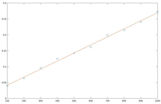
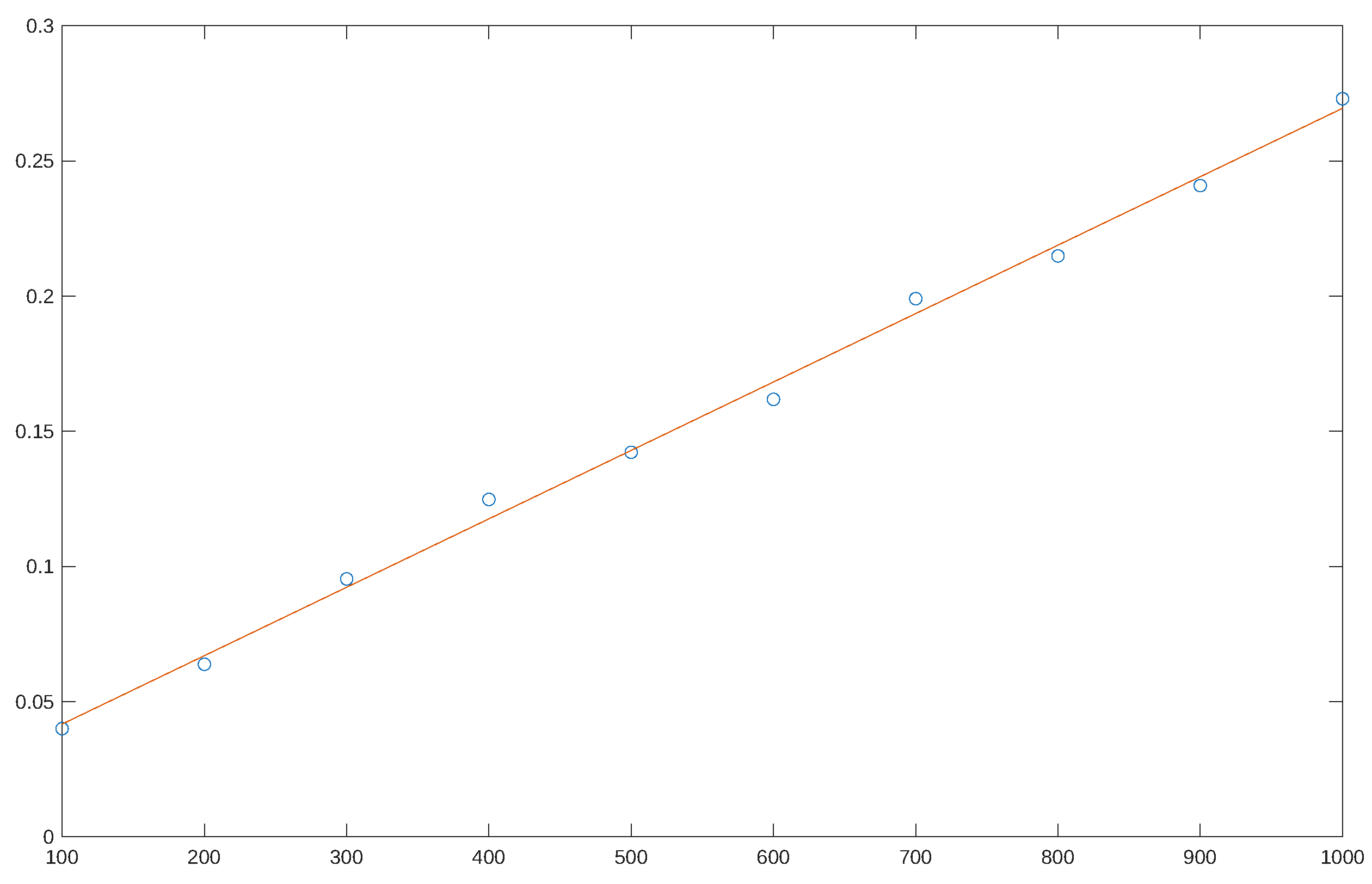
Figure 1 shows the execution times of our updating procedure when it is used to compute the triangular factorization of $B^2-0.5I$ for $n=100:100:1000$, starting from the triangular factor of $B^2$ represented via generators in quasiseparable form. The running times grow linearly with n, in agreement with the theoretical complexity estimates.

Figure 1. Runtime versus matrix size for the factorization updating algorithm. The linear fit is a good approximation of the measured data; its equation is $y=2.53\times {10}^{-4}x+0.0164$.

Procedure BISECTION is used to compute the eigenvalues of the matrix of size $n=1024$. It follows from the symmetry of the matrix that the eigenvalue problem is well conditioned. Therefore the MATLAB function eig, which implements a backward-stable algorithm, yields the most accurate numerical results. The input parameters are set to $a_0=0$, $b_0$ = $\Vert B^2{\Vert }_{\infty }$, $tol=b_0\mathtt{u}$, where $\mathtt{u}$ is the machine precision. The matrix $B^2$ has clustered eigenvalues located in the interval $[2.2,6.3]$. In (5) we show on the left the “exact” eigenvalues ${\lambda }_m$, $507\le m\le 513$, computed by the eig function of MATLAB, and on the right their approximations returned by Procedure BISECTION, together with the corresponding absolute errors. Since the eigenvalues of the leading principal submatrices interlace, by Cauchy’s theorem, the shifted matrices have several nearly singular leading principal submatrices close to convergence. Our method nevertheless behaves robustly. Only for the last two eigenvalues (marked with ★), and only at the last iteration, does the algorithm report a breakdown of the updating procedure. This premature termination does not affect the accuracy of the computed approximations.

$$\left[\begin{array}{c}3.999999999163282\\ 3.999999999571646\\ 3.999999999819462\\ 3.999999999946716\\ 3.999999999993500\\ 3.999999999999999\\ 4.000000000000000\end{array}\right]\left[\begin{array}{cc}3.999999999163284& 0.000000000000001\\ 3.999999999571647& 0.000000000000001\\ 3.999999999819471& 0.000000000000008\\ 3.999999999946712& 0.000000000000004\\ 3.999999999993499& 0.000000000000002\\ {4.000000000000000}_{★}& 0.000000000000001\\ {4.000000000000000}_{★}& 0.000000000000000\end{array}\right]$$

(5)

In the second experiment we set

$${\varphi }_k\left(x\right)=sin\left(2\pi kx\right),{\psi }_k\left(x\right)=2^{{\displaystyle 20(0.1+0.4(k-1)-x)}},k=1,2,3,$$

whereas the remaining parameters are as in the first experiment. The matrix $B^2$ now has entries of widely varying magnitude. Its eigenvalues lie in the interval $[0.5\times {10}^{-7},6\times {10}^7]$. In (6) and (7) we illustrate the convergence of our method when it approximates the three smallest and the three largest eigenvalues of $B^2$, respectively. Note that the Bauer-Fike theorem [17] predicts an absolute error of order $1.0\times {10}^{-8}$ for the computed eigenvalues. The measured errors agree with these conditioning estimates, which confirms the robustness of the method.

$$\left[\begin{array}{c}0.000000051827294\\ 0.038803790666506\\ 0.053418473649156\end{array}\right]\left[\begin{array}{cc}0.000000045516351& 0.000000006310943\\ 0.038803790515159& 0.000000000151347\\ 0.053418471720533& 0.000000001928623\end{array}\right]$$

(6)

$$\left[\begin{array}{c}888348.6868171052\\ 2074826.290225015\\ 54961816.03387247\end{array}\right]\left[\begin{array}{cc}888348.6868170921& 0.000000013038516\\ 2074826.290224833& 0.000000181840733\\ 54961816.03387250& 0.000000029802322\end{array}\right]$$

(7)

In the last experiment we consider

$${\varphi }_k\left(x\right)={\psi }_k\left(x\right)=sin\left(2\pi x\right),k=1,2,3;f\left(x\right)=x.$$

with the remaining parameters as above. Here $B^2$ is a singular diagonal-plus-rank-two matrix. Our implementation nevertheless makes use of a non-minimal quasiseparable representation of order 6. In (8) we report the results obtained by Procedure BISECTION for the five smallest eigenvalues of $B^2$. The approximations are as accurate as one can expect.

$$\left[\begin{array}{c}0.000000000000000\\ 0.000003822287905\\ 0.000015289663700\\ 0.000034402885181\\ 0.000061162695952\end{array}\right],\left[\begin{array}{cc}0.000000000000001& 0.000000000000001\\ 0.000003822287902& 0.000000000000003\\ 0.000015289663700& 0.000000000000001\\ 0.000034402885180& 0.000000000000001\\ 0.000061162695952& 0.000000000000000\end{array}\right]$$

(8)

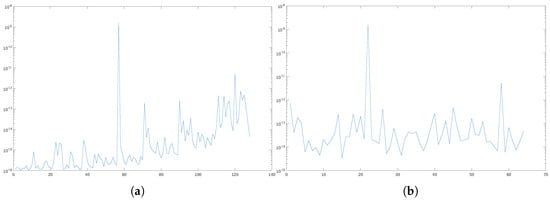
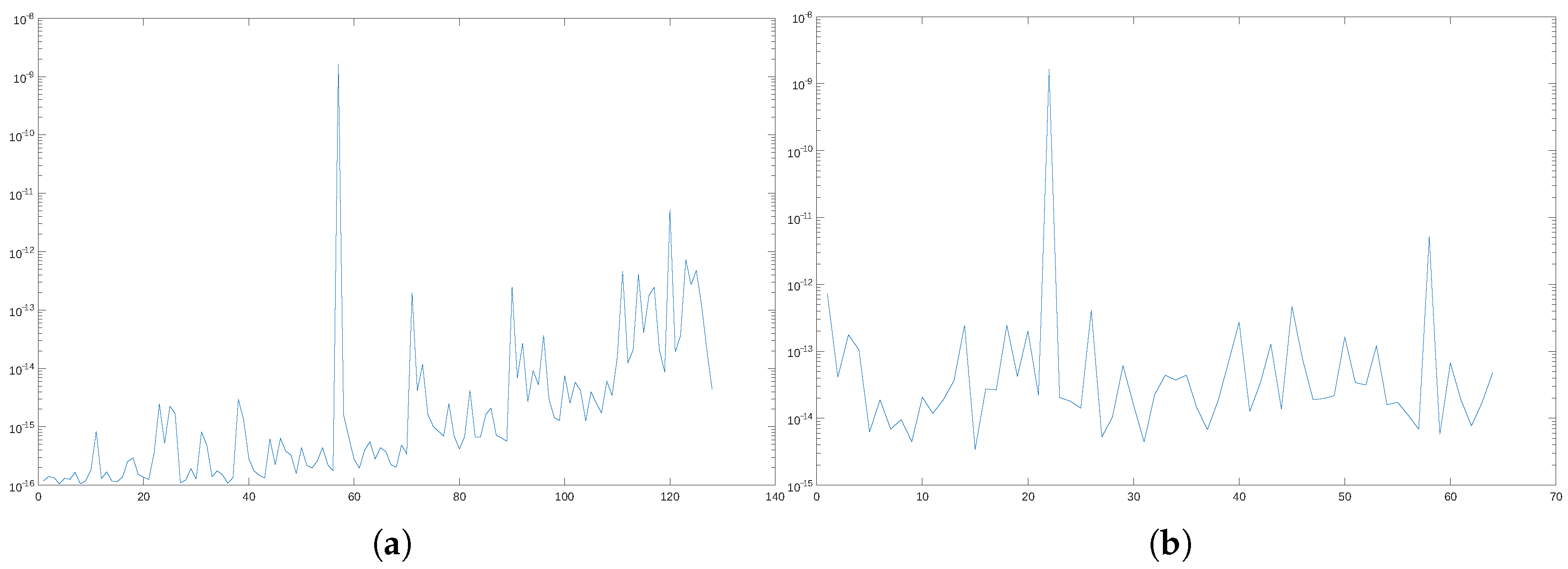
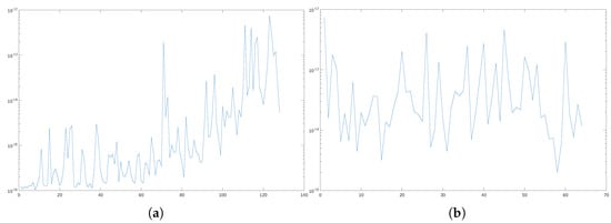
In the second scenario we have considered symmetric semiseparable matrices of size $n=128$ with generators of order $\kappa =3$ generated at random by means of the MATLAB function rand. Our bisection algorithm is used to compute all the eigenvalues of the input matrix. In Figure 2 we show the results obtained in the first $m=64$ cases (at the beginning of the experimental session the random number generator was initialized using the default generator algorithm and seed). In each experiment the “exact” eigenvalues of the input matrix are computed by the MATLAB function eig, and the absolute errors between these eigenvalues and the approximations $\widehat{\lambda }$ returned by our method are then evaluated. In $128\times 64=8192$ runs of Procedure BISECTION we observe only 3 (≃0.04%) premature breakdowns, all of them occurring where the matrix entries grow in magnitude to the order of $1.0\times {10}^7$. Only one of these, at iteration 22 in the computation of the 59-th eigenvalue of the input matrix, produces a significant deterioration of the measured absolute error.

Figure 2. Maximum measured absolute error per eigenvalue (a) and per iteration (b).

To avoid these accuracy problems, we propose the following modification. While the algorithm is running, we monitor the growth in magnitude of the entries of the generalized Givens matrices. If a prescribed threshold $maxgrowth$ is exceeded, the algorithm is restarted from a different starting point. In our implementation we set $maxgrowth=1.0\times {10}^5$ and, at the very beginning only, we take ${\alpha }_0=(2a_0+b_0)/3$. Figure 3 shows the results of this modified algorithm on the same test problems as in Figure 2. The results are now consistently accurate.

Figure 3. Maximum measured absolute error per eigenvalue (a) and per iteration (b) for the modified algorithm with the growth threshold.

6. Conclusions and Future Work

In this work we have designed a fast adaptation of the bisection method for computing the eigenvalues of symmetric matrices with quasiseparable structure. Numerical experiments are reported to confirm the robustness of the proposed algorithm when it is combined with a restarting technique. Our current research is mainly concerned with the design of a parallel algorithm for computing the eigenvalues of large symmetric quasiseparable matrices on concurrent processors while minimizing the communication between them. The parallel scheme retains the main structure of the sequential algorithm, and it exploits the multiprocessor environment by carrying out the required matrix factorizations concurrently. This approach has already proved to be very efficient for tridiagonal matrices [20]. It would also be of interest to compare the performance of implementations of parallel algorithms based on generalized Givens rotations and on Householder reflections for the updating of the triangular factorization of quasiseparable matrices.

References

- Vandebril, R.; Van Barel, M.; Mastronardi, N. Matrix Computations and Semiseparable Matrices. Volume II Eigenvalue and Singular Value Methods; Johns Hopkins University Press: Baltimore, MD, USA, 2008; pp. xvi+498. [Google Scholar]
- Eidelman, Y.; Gohberg, I.; Haimovici, I. Separable Type Representations of Matrices and Fast Algorithms. Volume 2 Eigenvalue Method; Operator Theory: Advances and Applications; Birkhäuser/Springer Basel AG: Basel, Switzerland, 2014; Volume 235, pp. xii+359. [Google Scholar]
- Eidelman, Y.; Haimovici, I. The bisection eigenvalue method for unitary Hessenberg matrices via their quasiseparable structure. Electron. Trans. Numer. Anal. 2023, 59, 60–88. [Google Scholar] [CrossRef] [Scilit]
- Eidelman, Y.; Haimovici, I. Bisection eigenvalue method for Hermitian matrices with quasiseparable representation and a related inverse problem. In Operator Theory, Analysis and the State Space Approach: In Honor of Rien Kaashoek; Springer International Publishing: Cham, Switzerland, 2018; pp. 181–200. [Google Scholar] [CrossRef] [Scilit]
- Fasino, D.; Gemignani, L. Direct and Inverse Eigenvalue Problems for Diagonal-Plus-Semiseparable Matrices. Numer. Algorithms 2003, 34, 313–324. [Google Scholar] [CrossRef] [Scilit]
- Utku, S. Sturm sequences or law of inertia of quadratic forms? Comput. Struct. 1973, 3, 419–420. [Google Scholar] [CrossRef] [Scilit]
- Horn, R.A.; Johnson, C.R. Matrix Analysis; Cambridge University Press: Cambridge, UK, 1985; pp. xiii+561. [Google Scholar] [CrossRef] [Scilit]
- Bojanczyk, A.; Qiao, S.; Steinhardt, A.O. Unifying unitary and hyperbolic transformations. Linear Algebra Appl. 2000, 316, 183–197. [Google Scholar] [CrossRef] [Scilit]
- Aurentz, J.L.; Vandebril, R.; Watkins, D.S. Fast Computation of the Zeros of a Polynomial via Factorization of the Companion Matrix. SIAM J. Sci. Comput. 2013, 35, A255–A269. [Google Scholar] [CrossRef] [Scilit]
- Uhlig, F. The DQR algorithm, basic theory, convergence, and conditional stability. Numer. Math. 1997, 76, 515–553. [Google Scholar] [CrossRef] [Scilit]
- Eidelman, Y.; Gohberg, I.; Haimovici, I. Separable Type Representations of Matrices and Fast Algorithms. Volume 1 Basics. Completion Problems. Multiplication and Inversion Algorithms; Operator Theory: Advances and Applications; Birkhäuser/Springer Basel AG: Basel, Switzerland, 2014; Volume 234, pp. xv+399. [Google Scholar]
- Eidelman, Y.; Gohberg, I. Out-of-band quasiseparable matrices. Linear Algebra Appl. 2008, 429, 266–289. [Google Scholar] [CrossRef] [Scilit][Green Version]
- Gohberg, I.; Lancaster, P.; Rodman, L. Matrices and Indefinite Scalar Products; Birkhäuser Verlag: Basel, Switzerland, 1983. [Google Scholar]
- Alexander, S.; Pan, C.T.; Plemmons, R. Analysis of a recursive least squares hyperbolic rotation algorithm for signal processing. Linear Algebra Appl. 1988, 98, 3–40. [Google Scholar] [CrossRef] [Scilit][Green Version]
- Gemignani, L. Solving Shifted Systems for Quasiseparable Matrices. arXiv 2026, arXiv:2606.26952. [Google Scholar]
- Eidelman, Y.; Gohberg, I. A modification of the Dewilde–van der Veen method for inversion of finite structured matrices. Linear Algebra Appl. 2002, 343–344, 419–450. [Google Scholar] [CrossRef] [Scilit]
- Golub, G.; Van Loan, C. Matrix Computations, 4th ed.; Johns Hopkins Studies in the Mathematical Sciences; Johns Hopkins University Press: Baltimore, MD, USA, 2013; pp. xiv+756. [Google Scholar]
- Boito, P.; Eidelman, Y.; Gemignani, L. Numerical solution of nonclassical boundary value problems. Numer. Algorithms 2025, 100, 745–768. [Google Scholar] [CrossRef] [Scilit]
- Aceto, L.; Gemignani, L. Computing the action of the matrix generating function of Bernoulli polynomials on a vector with an application to non-local boundary value problems. Adv. Comput. Math. 2025, 51, 19. [Google Scholar] [CrossRef] [Scilit]
- Chang, H.; Utku, S.; Salama, M. Eigenvalue computation of large symmetric tridiagonal matrices on concurrent processors. Comput. Struct. 1988, 29, 323–329. [Google Scholar] [CrossRef] [Scilit]
Disclaimer/Publisher’s Note: The statements, opinions and data contained in all publications are solely those of the individual author(s) and contributor(s) and not of MDPI and/or the editor(s). MDPI and/or the editor(s) disclaim responsibility for any injury to people or property resulting from any ideas, methods, instructions or products referred to in the content. |
© 2026 by the author. Licensee MDPI, Basel, Switzerland. This article is an open access article distributed under the terms and conditions of the Creative Commons Attribution (CC BY) license.