An Intelligent Distributed Adaptive Control Method for Multi-Channel Thermal Regulation in Fire-Resistance Testing Equipment

Abstract

Accurate regulation of combustion temperature is critical for objectively evaluating the fire-resistance performance of cables. However, existing temperature control strategies mainly rely on centralized regulation methods, which struggle to simultaneously address the nonlinear coupling among multiple heat sources, spatial thermal non-uniformity, and dynamic temperature fluctuations. To address these challenges, a multi-channel self-adaptive temperature control method based on distributed optimization and computational modeling is proposed in this study. First, a data-driven computational model based on an attention-enhanced multi-channel convolutional neural network is developed to characterize the complex nonlinear relationship between distributed heat inputs and the resulting temperature field, enabling accurate thermal state perception and prediction. Subsequently, a data-driven NSGA-III optimization algorithm is introduced to achieve dynamic allocation and coordinated optimization of heat flux among multiple independent heating channels. Furthermore, a deep reinforcement learning-based adaptive decision framework is established to realize autonomous adjustment of heating strategies under varying testing conditions. The proposed framework integrates thermal modeling, distributed optimization, and intelligent decision-making to achieve real-time adaptive control of multi-source heating systems. Experimental validation on practical fire-resistance testing equipment demonstrates that the proposed framework achieves an R² of 0.9745 with an MAE of 19.90 °C in the closed-loop control evaluation and provides improved spatial thermal uniformity compared with conventional control strategies.

1. Introduction

Ensuring the applicability of cables under fire scenarios is of great importance in modern society, as reliable cable operation can significantly reduce potential casualties and economic losses [1]. Various experimental approaches have been developed to evaluate the fire-resistance performance of cables. According to ISO 834, fire-resistance tests should be conducted using specialized testing equipment, where cables are exposed to standardized thermal conditions under controlled combustion temperatures [2,3]. However, maintaining a stable and uniform thermal environment remains challenging due to the coupled influence of multiple heat sources, nonlinear heat transfer behaviors, and dynamic testing conditions [4,5]. Therefore, developing an intelligent computational framework for modeling and adaptive regulation of multi-source thermal systems is essential for improving the reliability of cable fire-resistance evaluation.

Combustion temperature regulation has been extensively investigated by researchers and engineers [6,7,8]. In early studies, proportional-integral-derivative (PID)-based control strategies were widely applied owing to their simple structure and reliable performance [9,10]. Yao et al. coupled a computational fluid dynamics model with a PID controller to automatically regulate fire-induced smoke, investigating the influence of control distance on system robustness [11]. Feliu-Batlle and Rivas-Perez compared different PI-based and fractional-order control strategies for regulating the temperature of the combustion zone in industrial cement rotary kilns [12]. Zheng et al. integrated control theory, expert knowledge, fuzzy logic, and neural networks with PID control for furnace temperature regulation [13]. These studies demonstrate the effectiveness of PID-based approaches in conventional thermal systems. However, such methods generally rely on simplified input–output relationships and are insufficient for complex thermal systems involving multiple interacting heat sources [14,15,16,17].

In fire-resistance testing equipment, the temperature distribution is generated by the combined effects of multiple heating channels, where each heat source possesses independent operating parameters and contributes differently to the overall thermal field. Consequently, the temperature regulation problem can be regarded as a multi-variable thermal optimization problem involving coupled interactions among distributed heat inputs and spatial temperature responses. This characteristic significantly increases the complexity of conventional centralized control strategies.

With the rapid development of artificial intelligence and data-driven computing technologies, intelligent methods have been increasingly applied to thermal system regulation [18,19,20]. Among these approaches, reinforcement learning-based methods have attracted considerable attention owing to their adaptive decision-making capability under complex and dynamic environments. Brandi et al. employed deep reinforcement learning (DRL) to optimize supply water temperature control in heating systems through continuous interaction with the environment [21]. Taboga et al. developed an adaptive reinforcement learning framework to achieve temperature regulation across different building environments without repeated model training [22]. Wei et al. proposed a data-driven DRL-based strategy for intelligent operation of building heating and cooling systems [23].

Although reinforcement learning has demonstrated promising performance in various thermal control applications, its direct application to cable fire-resistance testing remains challenging. Two major issues should be considered.

(1)

Multi-point temperature regulation. Unlike conventional temperature-control problems with a single target, fire-resistance testing requires the temperatures measured by 32 spatially distributed thermocouples to simultaneously track the ISO 834 curve while maintaining spatial uniformity. Therefore, the control objective must account for both the overall tracking error and the temperature differences among multiple measurement locations.

(2)

Coupling among multiple heating sources. The furnace is heated by eight independently controlled heating channels. Although each channel has its own operating command, its thermal effect is not confined to a single measurement location because heat transfer, radiation, and thermal diffusion cause each source to influence multiple thermocouples. Therefore, coordinated regulation requires modeling the many-to-many coupling between the eight heating inputs and the resulting spatial temperature field.

To address these challenges, a multi-channel self-adaptive thermal control framework is proposed in this study. The proposed framework integrates computational modeling, multi-objective optimization, and adaptive control strategies. First, an attention-based multi-channel convolutional neural network is developed to establish the nonlinear mapping relationship between distributed heating inputs and temperature responses, providing a computational model for thermal state prediction. Subsequently, a data-driven NSGA-III optimization strategy is employed to achieve real-time multi-objective optimization of multiple heating channels, enabling coordinated adjustment of different heat sources. Finally, a deep reinforcement learning-based PID controller is developed to achieve adaptive regulation of individual heating sources under dynamic testing conditions. The main contributions of this study are summarized as follows:

(1)

An attention-based multi-channel thermal-field prediction model is developed to capture the many-to-many nonlinear relationship between eight heating-channel inputs and 32 spatial temperature responses. The model combines Bi-LSTM, scalar and vectorial attention, and multi-channel convolution to extract temporal dependencies and spatial coupling characteristics.

(2)

A hierarchical thermal-regulation method integrating NSGA-III, TOPSIS, and DQN is proposed. NSGA-III and TOPSIS determine the coordinated heat allocation among multiple heating channels, while DQN adjusts the actuator commands, enabling simultaneous ISO 834 curve tracking and spatial temperature-uniformity regulation.

(3)

A fully local multi-channel thermal-control system is implemented and validated on practical cable fire-resistance testing equipment. The proposed system achieves an MAE of 19.90 °C, an RMSE of 24.70 °C, and an $R^2$ of 0.9745 in closed-loop evaluation, demonstrating its feasibility for practical online thermal regulation.

The main novelty of this work lies in developing a surrogate-assisted hierarchical control mechanism that explicitly separates spatial heat allocation from actuator-level adaptive regulation and closes the loop between thermal-field prediction, multi-objective optimization, and physical control.

The remainder of this paper is organized as follows. Section 2 introduces the general framework, including control principles. A detailed introduction to the proposed method is presented in Section 3, and case studies are presented in Section 4. Finally, the conclusions of this study are presented in Section 5.

2. General Framework of Proposed Method

2.1. Problem Definition

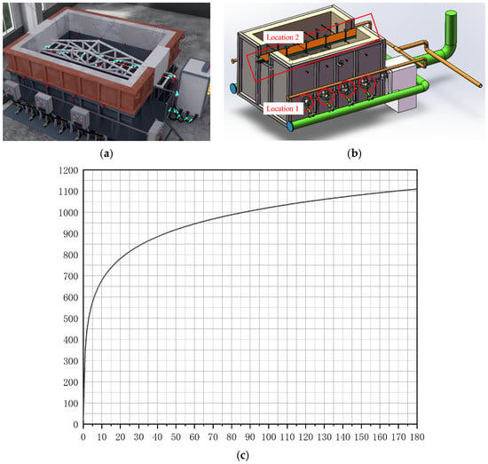
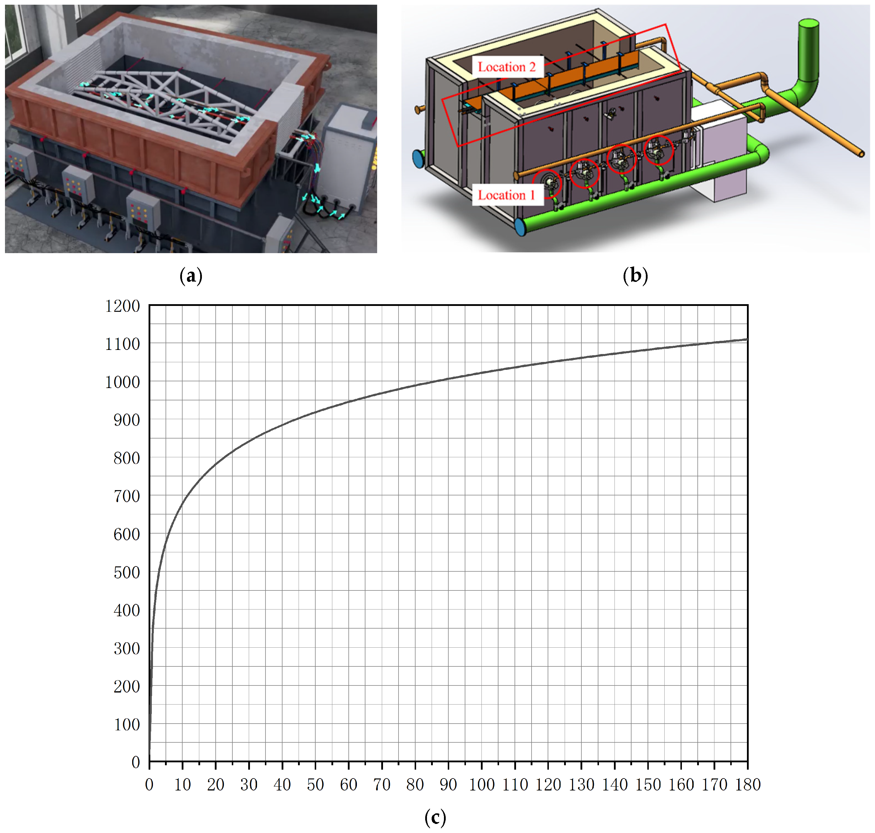
To clarify the motivation of this study, the general configuration of the cable fire-resistance testing equipment is illustrated in Figure 1. Figure 1a shows a three-dimensional view of the testing apparatus, which operates in a fully enclosed configuration during fire-resistance testing. The internal layout of the equipment is presented in Figure 1b. As indicated by the red area, i.e., location 2, the cable specimen is fixed at the central region of the furnace, where it is directly exposed to the thermal environment generated by the heating system. In particular, the test temperature for the cable is controlled by the eight combustion control ports, i.e., location 1. These eight control ports must work collectively to ensure that the temperature at location 2 remains constant and follows the standard heating curve shown in Figure 1c. Moreover, not only must the overall temperature at location 1 conform to the curve, but each individual point must also comply, thereby ensuring both overall temperature consistency and uniformity within the region. A detailed problem formulation is given below.

Figure 1. General structure of the cable fire-resistance testing equipment. (a) The 3D view of the general cable fire-resistance testing equipment. (b) The internal structure of the fire-resistance-testing equipment. (c) The ISO 834 standard temperature-rise curve [2].

During the testing process, the cable is subjected to thermal loading produced by multiple heating sources distributed symmetrically at the bottom of both sides of the furnace. Consequently, the temperature experienced by the cable is not governed by a single heat source but is instead the superposition of thermal effects from multiple burners. Under this multi-source heating condition, two fundamental challenges arise.

First, according to the fire-resistance testing standard ISO 834, the temperature near the cable must follow a prescribed standard temperature-rise curve, as shown in Figure 1c. However, in practical operation, the measured temperature is the result of the coupled effects of all heating sources, whose heat outputs are determined by a set of process variables. Any deviation in these variables may lead to a mismatch between the actual temperature evolution and the target ISO 834 curve. Therefore, the process variables must be continuously and coordinately adjusted to ensure that the resulting combustion temperature accurately tracks the standard temperature-rise law throughout the entire test duration.

Second, as illustrated in Figure 1b, the heating sources are spatially distributed on different sides of the furnace. This asymmetric spatial configuration inevitably introduces thermal non-uniformity in the vicinity of the cable. As a result, the local temperature around the cable fluctuates significantly around the standard temperature-rise curve. Statistical analysis of experimental data indicates that the temperature difference between the hottest and coldest regions near the cable can exceed 95 °C. Such severe thermal non-uniformity undermines the repeatability and reliability of the fire-resistance test, ultimately compromising the credibility of the testing results. Hence, maintaining thermal uniformity within an acceptable range is a critical yet unresolved issue in conventional cable fire-resistance testing systems.

In summary, effective temperature regulation requires addressing two distinct aspects: (i) modeling the dynamic relationship between the overall heating input and the spatially averaged furnace temperature to ensure accurate tracking of the ISO 834 temperature-rise curve; and (ii) characterizing the source-location-specific coupling between individual heating channels and multi-point temperature responses to coordinate heat allocation and maintain spatial thermal uniformity around the cable.

2.2. Detailed Workflow of Proposed Method

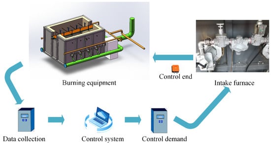
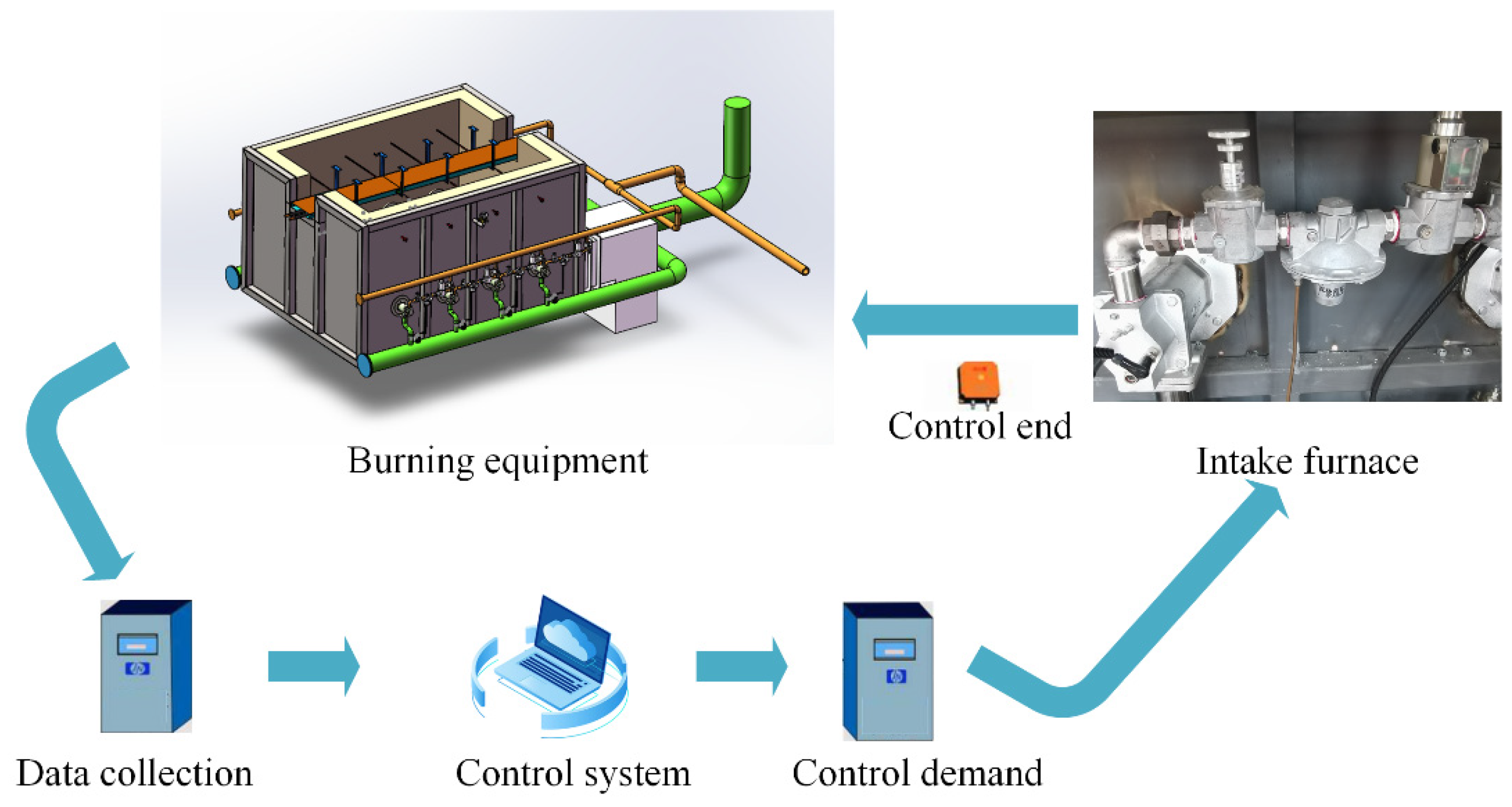
The flowchart of the proposed method is depicted in the Figure 2. It can be seen that the intake furnace provides the physical control action for the combustion equipment. During the combustion process, data are continuously collected to reflect the combustion temperature. Accordingly, the control system can be employed to provide parameter regulation, and gives demand orders to the physical intake furnace. By using this closed-loop reaction, the combustion temperature can be controlled in real-time.

Figure 2. Flowchart of the proposed method.

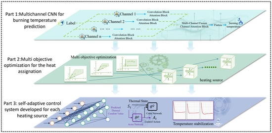
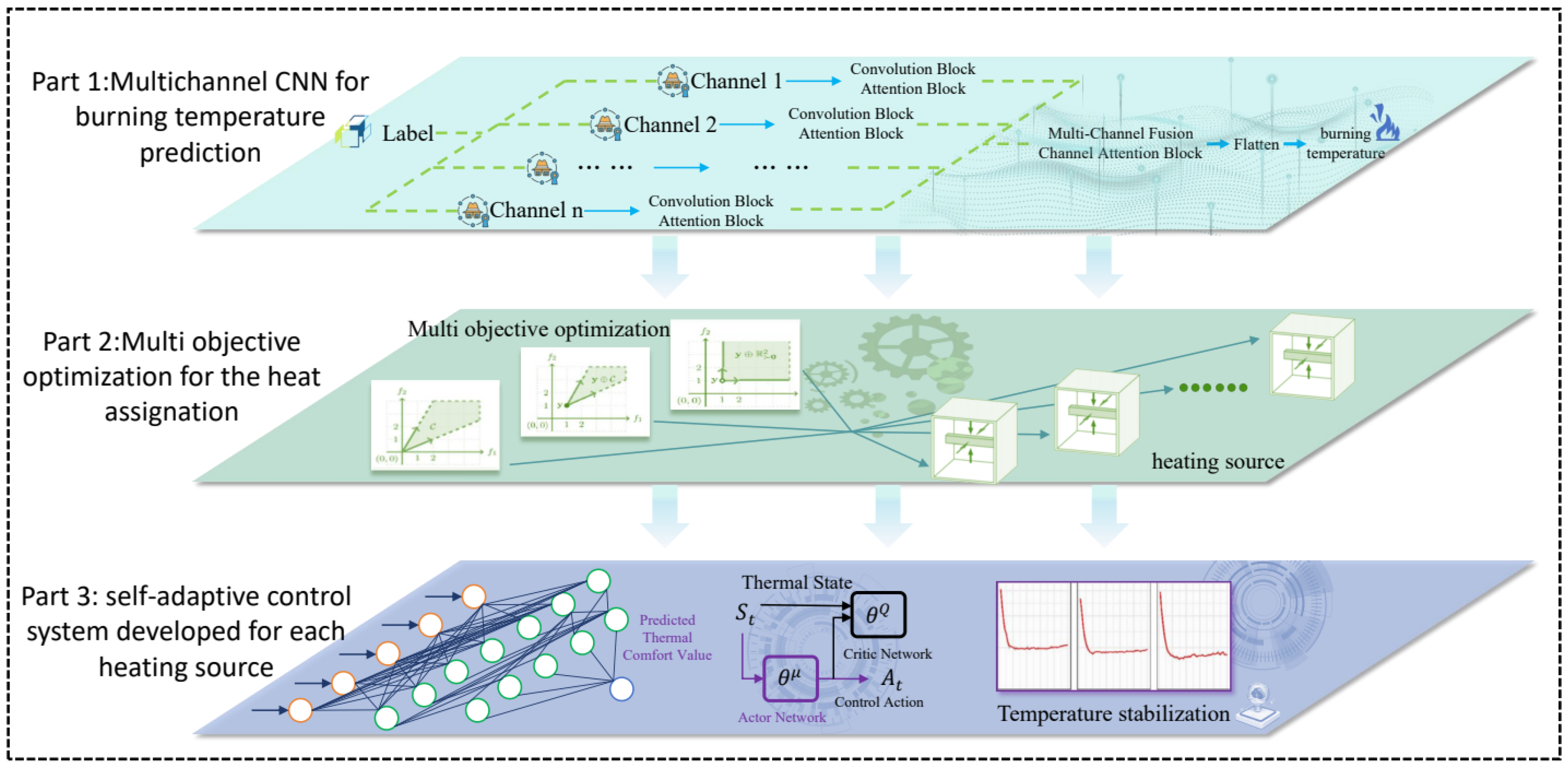
The general framework of the proposed method is shown in Figure 3. A multi-channel self-adaptive control method for the combustion temperature is proposed in this study, and it can be observed from the figure that there are three parts in the proposed method. The first part is a combustion-temperature prediction model that uses heating as the input. Subsequently, a multi-objective optimization algorithm is employed to assign a control target for each heating source. Finally, a self-adaptive control system developed for each heating source is employed to tune the variables in the heating source. Using these methods, the combustion temperature can be readily controlled.

Figure 3. The general framework of the proposed method.

As mentioned above, the first step in developing a multi-channel self-adaptive control system is the development of a combustion-temperature prediction model. In this study, a deep-learning technique called the multi-channel convolutional neural network is employed. The proposed attention-based multi-channel convolutional neural network is a type of convolutional neural network (CNN) variant that enhances the feature extraction ability from a time-scale perspective [24,25]. Using this neural network, the spatial and temporal features hidden in the heating source and combustion temperature can be extracted. Thus, a relationship between different heat sources and combustion temperatures can be developed.

Next, NSGA-III is employed to determine the heat allocation among the eight heating channels. A candidate solution is represented by

$$U^k\left(t\right)=[u_1^t\left(t\right),u_2^t\left(t\right),\dots ,u_8^t(t)]$$

where $u_k^t\left(t\right)$ denotes the candidate heat-input setpoint of the i-th heating channel. Each candidate must satisfy the actuator operating-range and command-variation constraints. For each candidate allocation, the AMCNN serves as a surrogate of the physical furnace. The candidate vector $U^k\left(t\right)$, together with the current temperature field and historical thermal state $X\left(t\right)$, is provided to the AMCNN to predict the temperature field at the 32 thermocouple locations. The predicted temperature field is then used to calculate two optimization objectives. The first objective minimizes the average tracking error relative to the ISO 834 target. The second objective minimizes spatial temperature non-uniformity.

Using the previous steps, the control target for each heat source can be readily obtained. The gap between the current output heat and the control target can then be realized. Using this information, improved deep reinforcement can be combined to adjust the process variables in the heating source in a self-adaptive manner. In contrast to conventional methods, improved deep reinforcement learning can tune process variables in a more efficient manner, which is more suitable for real-time control of the heating source.

3. Multi-Channel Self-Adaptive Control Method for Combustion Temperature

3.1. Attention-Based Multi-Channel CNN

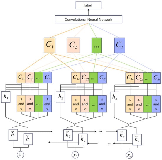
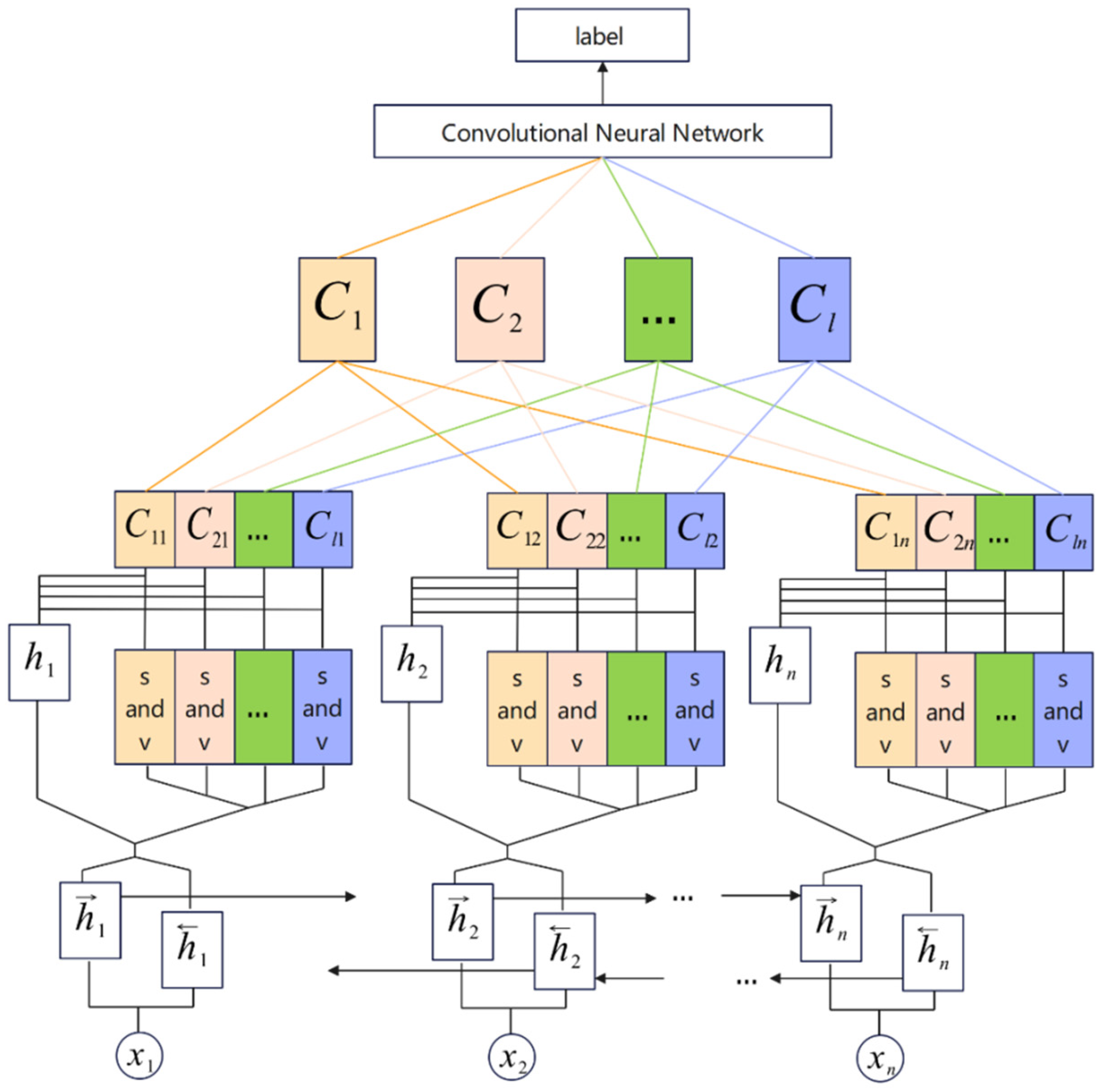
An attention-based multi-channel CNN (AMCNN) is employed in this study to construct a combustion-temperature prediction model. The proposed AMCNN is presented in Figure 4, and it can be observed from the figure that the AMCNN is composed of three parts, i.e., bi-directional long short-term memory (Bi-LSTM), an attention layer, and a CNN [26,27]. The raw input data are input into the Bi-LSTM first, and the Bi-LSTM is employed to generate scalar attention and vectoral attention. Finally, a multi-channel CNN can be developed using this type of attention. Using this AMCNN, the final developed model can be employed to represent long-term combustion temperature variations. Details regarding the construction of the AMCNN are introduced in the following subsections.

Figure 4. AMCNN structure.

Bi-LSTM is a variant of LSTM. Bi-LSTM is employed in this study to obtain annotations of the input vectors by extracting hidden features from both directions [28,29]. Generally, a Bi-LSTM contains backward and forward LSTM, denoted as $\overleftarrow{LSTM}$ and $\overrightarrow{LSTM}$. $\overleftarrow{LSTM}$ denotes the reading of the vectors from $x_n$ to $x_i$, and $\overrightarrow{LSTM}$ denotes the reverse operations. The mathematical formations of these two operations are as follows:

$$x_i=W_e{w}_i,i\in [1,n],$$

$$\overrightarrow{h_i}=\overrightarrow{LSTM}(x_i),i\in [1,n],$$

$$\overleftarrow{h_i}=\overleftarrow{LSTM}(x_i),i\in [1,n].$$

where $\overrightarrow{h_i}$ denotes the forward hidden state, which stores previous information, and $\overleftarrow{h_i}$ denotes the backward hidden state, which encodes information from later positions within the completed historical window. $x_i$ denotes the i-th input vector during the monitoring process; and $i$ denotes the time step.

The input and output definitions of the AMCNN are specified as follows. All heating-source operating variables and temperature measurements were synchronously acquired at a frequency of 10 Hz, corresponding to a sampling interval of $\Delta \mathrm{t}=0.1 \mathrm{s}$. At time step $i$, the input vector is defined as

$$x_i={\left[u_{1,i},u_{2,i},\dots ,u_{8,i},T_{1,i},T_{2,i},\dots ,T_{32,i},\right]}^T$$

where $u_{k,i}$ denotes the normalized heat-input command of the k-th heating channel and T_j,i denotes the temperature measured by the j-th thermocouple. Thus, both the eight heating-channel signals and the 32 thermocouple signals are used as model inputs. The heating signals characterize the thermal excitation applied to the furnace, while the historical thermocouple measurements characterize the current thermal state and thermal inertia of the furnace.

In Figure 4, the term “label” denotes the measured 32-dimensional temperature vector at t + 10, which is used only as the supervised prediction target during training. After the feature extraction performed using the Bi-LSTM, the attention mechanism is used to reflect the importance weight of the input element such that the relevant element contributes significantly to the merged output. In this study, two different attention mechanisms were jointly employed, i.e., the scalar attention mechanism and vectoral attention. These two attention mechanisms are jointly employed in the hidden states of the Bi-LSTM and are spliced into a matrix. In this manner, several matrices can be obtained, which can be considered as the multi-channel inputs of the CNN.

• Scalar Attention Mechanism

A scalar attention mechanism is employed to calculate the importance weights of the input data. To illustrate the scalar attention mechanism more clearly, the mathematical symbols are first unified. Here, M denotes the association matrix representing the association between the input data. The elements in the i-th row and j-th column denote the degree of association between the i-th and j-th data. We then assume that $L$ channels are required, and the L channel mask matrices are set as $V$. Therefore, $M_{l_{i,j}}$ can be obtained using the following formula:

$$M_{l_{i,j}}=\mathrm{t}\mathrm{a}\mathrm{n}\mathrm{h}([h_i,W_l·h_j]+b_l),$$

where l denotes the $l$-th channel, and the $i$-th channel mask matrix can be obtained as follows:

$$V_{l_{i,j}}\sim B(1,p_l),i\in [1,n],j\in [1,n],$$

where each element of $V_l$ follows the binomial distribution. Under the circumstance of $M_{l_{i,j}}$ and $V_{l_{i,j}}$, the $i$-th channel can be obtained using the following formula:

$$A_l=M_l\otimes V_l,$$

$$s_{lk}=\sum _x{A}_{l_{xk}},$$

$$p_k=\left\{\begin{array}{cc}-\mathrm{99,999},& if x_k is from pad\\ 0,& otherwise\end{array}\right.$$

$$scor{e}_{lk}=p_k+s_{lk},$$

$$a_{lk}={\displaystyle \frac{\mathrm{e}\mathrm{x}\mathrm{p}\left(scor{e}_{lk}\right)}{{\sum }_{i=1}^n\mathrm{e}\mathrm{x}\mathrm{p}\left(scor{e}_{li}\right)}},$$

$$c_{li}=a_{li}·h_i,$$

$$C_l=\left[c_{l1},c_{l2},c_{l3},\cdots \cdots ,c_{ln}\right].$$

where $c_{li}$ is the new representation of $h_i$ in the $l$-th channel; $\otimes$ indicates the element-wise product operation; and the symbol $pad$ indicates the little information recorded using Bi-LSTM.

The scalar attention mechanism operates along the temporal dimension. For the $l$-th attention channel, it generates one scalar weight $a_{l,i}^s$ for each time step $i$. The scalar weight is applied uniformly to all dh components of the corresponding hidden state. Therefore, scalar attention identifies the relative importance of the 100 historical time steps but does not distinguish among the hidden-feature components within the same time step.

• Vectorial Attention Mechanism

For vectorial attention, the input is the Bi-LSTM hidden-state sequence rather than the raw heating-source vector. Each hidden component is assigned its own temporal attention distribution. Based on these definitions, the vectorial importance weight of each heat source in the input element can be calculated as follows: ${\left(v_1,v_2,v_3,\dots ,v_n\right)}^T$

$$\begin{array}{c}\overrightarrow{scor{e}_{li}}={W_{l1}}^T\sigma \left(W_{l2}·h_i+b_l\right),\hfill \\ \overrightarrow{a_{li}}={\displaystyle \frac{\exp \left(\overrightarrow{scor{e}_{li}}\right)}{{\sum }_i\mathrm{e}\mathrm{x}\mathrm{p}\left(\overrightarrow{scor{e}_{li}}\right)}},\hfill \\ c_{li}=\overrightarrow{a_{li}}\odot h_i,\hfill \\ C_l=\left[c_{l1},c_{l2},c_{l3},\cdots ,c_{ln}\right].\hfill \end{array}$$

where $c_{li}$ is the final presentation of $h_i$ in the $l$-th channel. By concatenating all $c_{li}$, where $i\in [1,n]$, the $l$-th channel can be obtained, which is denoted as $C_l$.

Using a combination of scalar and vectorial attention, the multi-channel is obtained as follows:

$$\begin{array}{c}{c}_{li}=a_{li}·(\overrightarrow{a_{li}}\odot h_i),\hfill \\ C_l=[c_{l1},c_{l2},c_{l3},\cdots ,c_{ln}]\hfill \end{array}$$

In summary, scalar attention assigns one temporal importance weight to each historical step, whereas vectorial attention assigns component-specific temporal weights to the latent features. Their fusion enables the AMCNN to retain complementary temporal and latent-feature information for temperature-field prediction.

In the next step, the multi-channel CNN is introduced. It is assumed that one channel is represented as

$$C=[c_1,c_2,c_3,\dots ,c_n]$$

where n denotes the length of the input element; in terms of the multi-channel, it is denoted as the multiple input for the obtained data. In the CNN modeling phase, a max-pooling operation is employed.

Although the AMCNN contains a bidirectional recurrent structure, it does not require future measurements during real-time operation. At the current decision time t, the model receives a completed historical window containing the observations from t − 99 to t. The forward LSTM reads the window chronologically, whereas the backward LSTM reads the same historical window in reverse order. Accordingly, the latest measurement accessible to both recurrent directions is $x_t$. Measurements after time t, including $x_{t+1}$, are not accessible to the model.

It should be emphasized that “bidirectional” refers to the processing directions within the available historical window rather than access to observations occurring after the control decision. The backward LSTM can use $x_t$ when encoding an earlier position such as $x_{t-20}$; however, $x_t$ has already been measured when the prediction is made. Therefore, this operation does not violate real-time causality. The online prediction process is expressed as

$${\widehat{Y}}_{t+10}=f_{AMCNN}(x_{t-99},\dots ,x_t),$$

where ${\widehat{Y}}_{t+10}$ is the predicted temperature field 1 s ahead. A first-in-first-out rolling buffer is used to store the latest 100 observations. Following the initial 10 s buffer-filling period, the buffer is updated every 0.1 s by removing the oldest observation and appending the latest heating-channel and thermocouple measurements. The AMCNN subsequently generates a new prediction at each sampling instant without introducing an additional 10 s waiting period. During the initial buffer-filling period, the equipment follows the predefined safe heating trajectory under conventional feedback control. AMCNN-based predictive control is enabled only after 100 valid observations have been collected.

Unlike scalar attention, the vectorial attention mechanism generates a $d_h-dimensional$ attention vector for each time step. For each hidden-feature component q, the attention weights are normalized over the n historical time steps:

$$c_{l,i}^v=a_{l,i}^v\odot h_i$$

where ⨀ denotes element-wise multiplication. Thus, vectorial attention provides a component-specific temporal weight for each latent feature, allowing different hidden-feature components to emphasize different portions of the historical window.

3.2. Surrogate-Assisted NSGA-III for Heat Allocation

The heat-assignment problem is formulated as a constrained bi-objective optimization problem. A candidate solution is an eight-dimensional heat-allocation scheme, in which each decision variable represents the heat-input setpoint assigned to one of the eight independently controlled heating channels. The search space consists of all heat-allocation schemes that satisfy the allowable operating range of each actuator and the maximum permitted variation between consecutive control commands. For each candidate solution, the AMCNN serves as a surrogate of the physical furnace and predicts the resulting temperatures at the 32 thermocouple locations. The first objective is to minimize the average deviation between the predicted temperatures and the ISO 834 target temperature. The second objective is to minimize spatial temperature non-uniformity among the 32 thermocouple locations. NSGA-III therefore searches for Pareto-optimal heat-allocation schemes that simultaneously improve temperature tracking accuracy and spatial thermal uniformity.

At this stage, a previously developed combustion-temperature prediction model is employed as a surrogate model for the optimization stage. Multiple genetic algorithms exist for the optimization process. Among these genetic algorithms, the NSGA-III is considered to be the most suitable and advanced algorithm employed in this study [30,31]. NSGA-III was proposed by Deb and Jain and demonstrated excellent performance in terms of computation cost [32]. Using this advantage, NSGA-III can be employed for the online optimization of variables in different application scenarios. Using NSGA-III, the distributed Pareto-optimal solutions of the heating source can be obtained owing to its high computational efficiency. Using NSGA-III, the heat assigned to each source can be obtained online.

The pseudocode for the NSGA-III is presented in Algorithm 1. The code for the Pareto fronts are required to be generated first, and all populations are ranked using these Pareto fronts. The first front comprises all non-dominated individuals within the current population, while the second front encompasses individuals dominated by those belonging to the first front. This distribution plays a role in selecting the solutions until the number of individuals required to form the next generation is attained. If the last front to be added contains more individuals than required, a selection must be made within this front using a reference line. The reference line originates from the center and passes through the reference point. Solutions with a minimum perpendicular distance to the reference line are prioritized during selection. Finally, the selected population contains feasible heat-allocation vectors evaluated according to ISO 834 tracking error and spatial temperature non-uniformity.

In general, during the application phase, a set of Pareto front solutions is generated. However, in these Pareto front solutions, it can be difficult for operators or machines to select the types of parameters that need to be considered on the machine. To make this method more convenient, TOPSIS is employed in this study. Typically, multiple Pareto optimal solutions exist. Considering the computational efficiency and variety of calculated objectives, a technique for order performance by similarity to an ideal solution is employed in this study. This technique is a multi-criteria decision-making method that determines alternatives and criteria to make an approximate decision from the potential solutions. TOPSIS was first proposed by Hwang and Yoon in 1981; its main pseudocode is presented in Algorithm 2 [33].

Algorithm 1 Pseudo code of NSGA-III

Input      $P_0$ (Initial Population)      $N_{\mathrm{pop}}$ (size of population)      $t$ (iteration = 0)      ${It}_{\max }$ (Maximum iteration)   While $t<{It}_{\max }$ do      Create Offspring $Q_{\mathrm{t}}$      Mutation on $Q_{\mathrm{t}}$      Set $R_{\mathrm{t}} = P_{\mathrm{t}} \cup Q_{\mathrm{t}}$      Apply non-dominated sorting on $R_{\mathrm{t}}$ and find $F_1,F_2,\dots$      $S_{\mathrm{t}} = \left\{\right\}, i = 1;$      WHILE $\mid S_{\mathrm{t}}\mid \le N_{\mathrm{pop}}$ DO      $S_{\mathrm{t}} = S_{\mathrm{t}} \cup F_{\mathrm{i}}$      $i = i + 1$     End     ELIF $\mid S_{\mathrm{t}}\mid = N_{\mathrm{pop}}$ DO          $P_{\mathrm{t}+1} = S_{\mathrm{t}};$ break     ELSE       $P_{\mathrm{t}+1}=U_{j=1}^{l-1}{F}_{\mathrm{j}}$       Normalize $S_{\mathrm{t}}$ using min and intercept points of each objective       Associate each member of $S_{\mathrm{t}}$ to a reference point       Choose $N_{\mathrm{pop}}-\mid P_{\mathrm{t}+1}\mid$ members from $F_{\mathrm{i}}$ by niche-preserving operator      END      $t = t + 1$  END  Report $P_{\mathrm{t}}$ (Pareto Solution sets)

Algorithm 2 demonstrates that the distance between the positive and negative solutions is calculated initially. In this study, the positive and negative ideal solutions are defined from the normalized best and worst values of the two objectives: ISO 834 tracking error and spatial temperature non-uniformity. TOPSIS essentially involves the identification of the solution that is closest to the positive and farthest from the negative in terms of relative distance. It is necessary to assign weights, denoted as $w_j$, to each criterion. These weights are typically determined based on operator preferences and can be adjusted to align with different operational requirements.

In this section, a data-driven surrogate, the NSGA-III, is proposed. In general, the proposed method first employs a previously developed combustion-temperature prediction model as a surrogate model for the optimization process. In the multi-objective optimization stage, NSGA-III is employed to generate Pareto solutions according to the actual working conditions. In particular, considering that there would be a set of Pareto solutions during the optimization phase, TOPSIS is used to find the best solution from these answers. Thus, the heat assigned to each heating source can be obtained in a highly efficient manner, which can be applied to control the combustion temperature.

Algorithm 2 Pseudo code of TOPSIS

1. Construction of normalized decision matrix $r_{ij}={\displaystyle \frac{x_{ij}}{\sqrt{{\sum }_{i=1}^m{x}_{ij}^2}}}\forall j$ where $r_{ij}$ denotes the elements of normalized decision matrix 2. Construction of weighted normalized decision matrix $v_{ij}=r_{ij}\ast {\omega }_j\forall i,j$ where ${\omega }_j$ denotes the assigned weight to attribute $j$ 3. Determination of ideal $\left({\mathcal{A}}^{+}\right)$ and negative-idea $\left({\mathcal{A}}^{-}\right)$ solutions ${\mathcal{A}}^{+}=\left\{\left(\underset{j}{\max } v_{ij}|i\in I\right),\left(\underset{j}{\min } v_{ij}|i\in I^{\prime }\right);\forall j\right\}=\left\{v_1^{+},v_2^{+},\dots \right\}$ ${\mathcal{A}}^{-}=\left\{\left(\underset{j}{\min } v_{ij}|i\in I\right),\left(\underset{j}{\max } v_{ij}|i\in I^{\prime }\right);\forall j\right\}=\left\{v_1^{-},v_2^{-},\dots \right\}$ where I and $I^{\prime }$ are associated with benefit and cost attributes respectively. 4. Calculation of separation measure $S_i^{+}=\sqrt{{\displaystyle \sum _{i=1}^n}{\left(v_{ij}-v^{+}\right)}^2}\hspace{1em}\forall j$ $S_i^{-}=\sqrt{{\displaystyle \sum _{i=1}^n}{\left(v_{ij}-v^{-}\right)}^2}\hspace{1em}\forall j$ 5. Calculation of relative closeness to the ideal solutions $C_j^{+}={\displaystyle \frac{s_j^{+}}{s_j^{+}+s_j^{-}}}$ Ranking of alternatives based on $C_j^{+}$ values

In the proposed two-stage decision process, NSGA-III first generates a set of Pareto-optimal heat-allocation solutions, and TOPSIS subsequently selects one preferred solution for implementation. NSGA-III searches for diverse trade-offs between ISO 834 temperature tracking and spatial temperature uniformity without combining the two objectives into a single weighted objective during the optimization process. This prevents the search from being prematurely restricted by predefined weights and preserves alternative solutions, particularly when the objectives are conflicting or the Pareto front is nonlinear or non-convex.

TOPSIS is applied only after the Pareto set has been obtained. Its criterion weights are used to rank the non-dominated solutions according to their relative closeness to the ideal operating condition, rather than to guide the generation of candidate solutions. Therefore, NSGA-III provides a representative set of feasible trade-offs, while TOPSIS converts this set into a single executable heat-allocation command. Compared with direct scalarization, this separation improves the transparency and flexibility of the decision process because operational preferences can be adjusted at the final selection stage without changing the underlying multi-objective search.

The multi-channel thermal regulation problem is formulated as a hierarchical optimization-control problem involving multiple heating sources and spatially distributed temperature responses. In the investigated fire-resistance testing equipment, eight independent heating channels are employed to regulate the temperature field around the cable. The input vector of the heating system is defined as $U\left(t\right)=[u_{1\left(t\right)},u_{2\left(t\right)},\dots ,u_{8\left(t\right)}]$, where $u_{i\left(t\right)}$ represents the heat input of the $i$-th heating channel determined by the actuator operating conditions.

The corresponding thermal response is represented by the spatial temperature field $Y\left(t\right)=[T_{1\left(t\right)},T_{2\left(t\right)},\dots ,T_{32\left(t\right)}]$, where $T_{j\left(t\right)}$ denotes the temperature measured by the j-th thermocouple. Due to heat transfer interaction, radiation coupling, and spatial thermal diffusion, the relationship between heating inputs and temperature responses is highly nonlinear and can be expressed as $Y\left(t\right)=F\left(U\right(t),X(t\left)\right)$, where X(t) represents the thermal state information including current temperature distribution, temperature deviation, previous control actions, and thermal evolution history.

Two objectives are considered in the NSGA-III-based heat allocation process. The first objective is thermal consistency with the ISO 834 standard temperature-rise curve, which minimizes the temperature tracking error:

$$f_1=({\displaystyle \frac{1}{N}})\sum \mid Tj(t)-TISO(t)\mid$$

The second objective is spatial thermal uniformity, which minimizes the temperature difference among different measurement locations:

$$f_2=max\left(Tj\right(t\left)\right)-min\left(Tj\right(t\left)\right)$$

Therefore, the multi-objective optimization problem is formulated as minimizing F = [f1, f2]. Additionally, physical constraints are imposed to guarantee safe operation:

$$u_{i\left(min\right)}\le u_{i\left(t\right)}\le u_{i\left(max\right)}$$

$$\mid ∆u_{i\left(t\right)}\mid \le ∆u_{i\left(max\right)}$$

where $u_{i\left(min\right)}$ and $u_{i\left(max\right)}$ represent the allowable operating range of each heating actuator, and ∆ui(max) limits the maximum variation in actuator commands.

The coupling relationship among multiple heating channels is considered through the AMCNN surrogate model. Instead of independently optimizing each heating source, NSGA-III searches the optimal heat allocation vector by considering the combined influence of all heating channels on the predicted spatial temperature field. Consequently, the Pareto solutions obtained simultaneously satisfy ISO 834 temperature tracking requirements and spatial thermal uniformity requirements.

In the reported implementation, NSGA-III used a population size of 100 and 200 generations to optimize two objectives over eight decision variables. Each candidate was evaluated by the AMCNN surrogate and was rejected if it violated the actuator operating range or maximum command-variation constraint.

3.3. Improved Deep-Reinforcement-Learning-Based Tuning Skill

In this section, improved DRL is employed to control the output heat to realize self-adaptive control of the combustion temperature. The proposed method takes into consideration Q-learning, which can help control the combustion temperature from an end-to-end perspective. In contrast to conventional methods that comprise a control application using a predefined parameter set by operators, the control agent in the proposed method directly learns the optimal policy or control principle from its interactions with the environment through a delayed reward mechanism [34,35]. Using DRL, a control agent can be applied to complex control problems that are difficult to solve using conventional methods. In addition, DRL can be applied automatically, which is helpful for operators who have little experience. Owing to these advantages, the DRL is employed to control the process variables in the heating source of the fire-resistance testing equipment.

When the DRL is applied to the heat control, an agent (e.g., a control module linked to the heating source of the fire-resistance testing equipment and running locally on the control workstation performs an action (e.g., tuning the process variables) when the environment (e.g., the assigned heat in the previous step) is in a stage (e.g., the output heat differs from the desired setpoint) and obtains a reward that denotes how well the agent performs by using that action in that state related to control objectives. The main purpose of the agent is to learn the optimal $policy \left(\pi \right)$, which maps the stage and the probability of each action being selected. The stage value function, which denotes the expected return (e.g., the cumulative sum of future rewards) of the agent when starting from state s and following policy $\pi$, and it can be obtained as follows:

$$v_{\pi }\left(s\right)=E[r_{t+1}+\gamma v_{\pi }(s^{\prime })\mid S_t=s,S_{t+1}=s^{\prime }]$$

where $\gamma$ denotes the discount factor for future rewards. Additionally, the action-value function, which is marked as the expected return of the agent when selecting an action starting from state s and following policy $\pi$, is as follows:

$$q_{\pi }(s,a)=E[r_{t+1}+\gamma q_{\pi }(s^{\prime },a^{\prime })\mid S_t=s,A_t=a]$$

Typically, the $v_{\pi }$ and $q_{\pi }$ are learned directly from experience. The DRL can be constructed by defining the above terms. In this study, a model-free DRL method called Q-learning is employed. In the Q-learning application phase, state-action values called Q-values are first estimated using existing experience. These values were calculated using the following formula:

$$Q(s_t,a_t)\leftarrow Q(s_t,a_t)+\alpha \left[r_t+\gamma ma{x}_{a}Q(s_{t+1},a)-Q(s_t,a_t)\right]$$

where $\alpha$ denotes the learning rate, and it is employed to determine the extension of new knowledge overrides old knowledge.

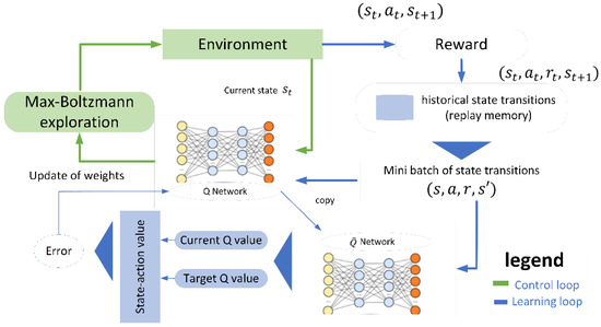
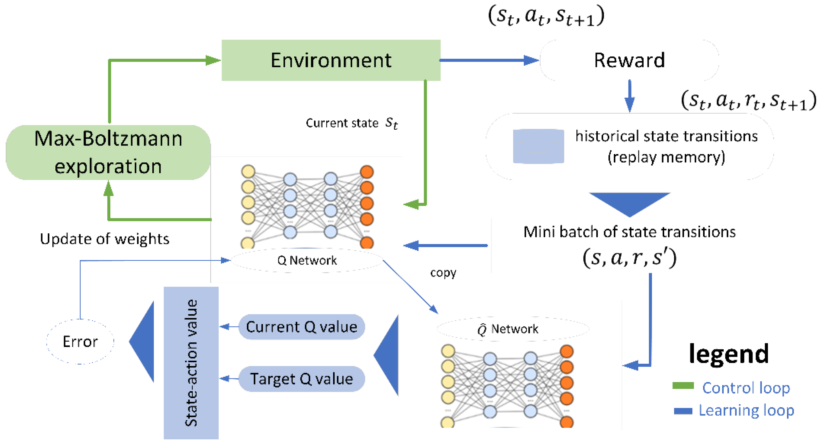
The entire Deep Q-learning framework is presented in Figure 5. As shown in the figure, the proposed Deep Q-learning method comprises two loops, i.e., a control loop and a learning loop. During offline training, the Max–Boltzmann rule is used for exploration; exploration is disabled during physical deployment, where the greedy action is applied after safety filtering. The system operates in a nearly deterministic manner when the estimations of the Q-values are unambiguous; however, they facilitate more extensive exploration in state-action space areas where the Q-value estimations are ambiguous. According to the Max–Boltzmann rule, the agent with probability ε selects actions with probabilities related to their Q-values and can be obtained as follows:

$$Pr\left(a\mid s\right)={\displaystyle \frac{e^{\frac{Q(s,a)}{\tau }}}{\Sigma e^{\frac{Q(s,a)}{\tau }}}}$$

where $\mathsf{\tau }$ denotes the Boltzmann temperature constant. As shown in Figure 5, a network is also involved in this structure, which is employed to develop an effective representation of the problem through its hidden layer. In the proposed deep Q networks, the Q-value function is parameterized by ϑ, which denotes the weights of the network. The neurons in the input layer were employed to represent the number of heating source variables. The output layer is employed to represent the possible actions that the agent may take in each control behavior. By using these deep Q networks, the proposed method can adaptively learn the relationship between the states and the Q-value for each action.

Figure 5. The structure of deep reinforcement learning with a Q-learning part.

Accounting for the learning process, it is initialized with high values of $\mathsf{\epsilon }$, and it would be gradually reduced to exploit obtained knowledge. To clarify the proposed method, its training process is introduced in this study. In general, many hyperparameters exist in reinforcement learning agents, and the fine-tuning of these parameters is often required. Hence, a sensitivity analysis was performed on the important hyperparameters through training based on different configurations to determine the variations in the obtained results. The training process is conducted from an offline perspective, and a training episode, which denotes the time period representative of controlling the process variables in the heating source, was employed multiple times to refine the agent’s control strategy. The sensitivity analysis is performed on the implemented agents for variable sets.

The DQN is trained offline using historical operating data and simulated/recorded state transitions rather than through unconstrained exploration on the real furnace. Each training episode corresponds to a complete control trajectory or a fixed-length segment of the heating process. Mini-batches sampled from replay memory are used for network updating. Training is terminated when the moving-average episode reward and the heat-target tracking error remain stable over successive validation episodes. The final network parameters are selected using the validation data and are fixed before physical deployment. The exact number of training episodes and convergence window used in the implementation are reported in Table 1.

Table 1. DQN training and implementation settings.

Item	Setting/Implementation Definition
State space	Assigned heat target; current heat output; target-tracking error; representative temperature state; ISO 834 temperature deviation; previous actuator command
Discrete action space	Three actions: decrease/maintain/increase
Action-to-command mapping	u(t + 1) = clip[u(t) + a · Δu]; a ∈ {−1, 0, +1}; Δu = 2% of actuator full scale per decision step
Reward	All error terms are normalized. r = −(0.40 · heat-target error2 + 0.35 · ISO 834 temperature error2 + 0.15 · spatial non-uniformity + 0.10 · actuator-change2); safety violation penalty = −10
Exploration strategy	Max–Boltzmann during offline training; ε starts at 1.0, decays by 0.997 per episode to a minimum of 0.05; Boltzmann temperature τ = 1.0; exploration disabled during physical deployment
Q-network hidden layers	Two fully connected hidden layers: 128 and 64 neurons
Activation function	ReLU in hidden layers; linear Q-value outputs
Learning rate/discount factor	Adam optimizer; learning rate = 1 × 10−4; discount factor γ = 0.98
Replay memory	Capacity = 100,000 transitions; mini-batch size = 128
Target-network update	Hard update every 500 gradient steps
Training episodes	2000 offline training episodes
Safety constraints	Actuator command limited to 0–100% of allowable range; command variation limited to ±2% full scale per decision step; commands violating actuator or furnace thermal-safety limits are clipped/rejected before execution
Convergence criterion	Training stops after 2000 episodes or earlier when the 100-episode moving-average reward changes by <1% and validation heat-tracking error changes by <1% for three consecutive evaluation windows; zero safety violations required on validation runs

The heat allocation selected by TOPSIS is used as the target heat-input setpoint for each channel and is included in the DQN state together with the current heat output and target-tracking error. Because the target and its error are state variables, the same offline-trained policy can accommodate each newly generated feasible allocation without retraining or fine-tuning. For each channel, the network outputs three Q-values corresponding to decrease, maintain, and increase actions; the selected increment is converted to a continuous actuator command and checked by the safety layer before execution.

In conclusion, through the existing interaction behavior in the proposed deep Q-learning, the proposed method can automatically learn the control rules for process variables in an automatic manner. Execution safety is enforced by the actuator-range, command-rate, and furnace thermal constraints summarized in Table 1; unsafe actions are rejected or projected onto the feasible command range before transmission.

4. Case Study

This section provides the details concerning the implementation of the proposed method and describes the experimental setup. In particular, actual equipment is employed. To comprehensively test the proposed method, its prediction accuracy is discussed in this section. Finally, a comparison between the proposed and conventional methods is presented in Section 4.3.

4.1. Experiment Settings

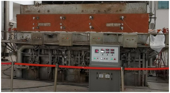
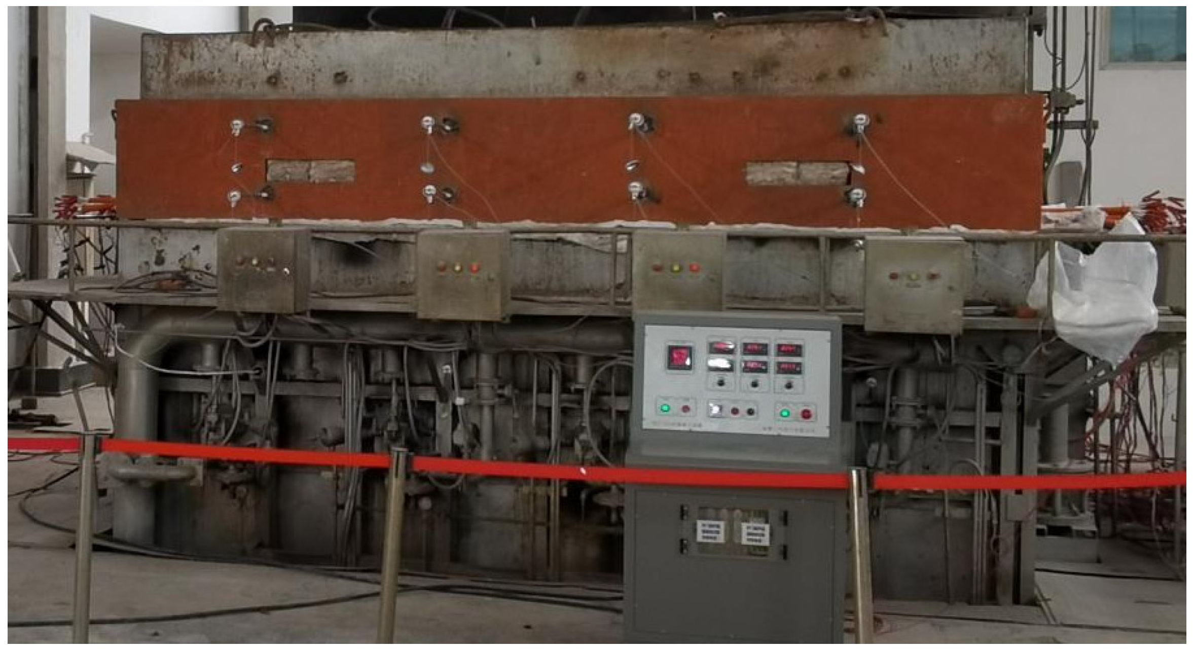
The general experimental illustration of the case is presented in Figure 6; it can be determined that a total of 32 thermocouples is fixed in the equipment, and those 32 thermocouples employed provide the detailed temperature value during the testing stage. Approximately 420 GB of raw experimental data were collected over three years, including heating-source operating variables and the corresponding multi-point temperature measurements.

Figure 6. Photograph of the experimental fire-resistance testing setup.

During the three-year period, 286 independent fire-resistance test runs were retained after data-quality screening. The data acquisition frequency was 10 Hz for both the heating-source operating variables and temperature measurements. Among these experiments, 240 runs corresponded to normal operating conditions, while 46 runs contained identifiable interruption or abnormal thermal disturbances, such as transient deviations of the measured temperature from the expected heating trajectory.

The 32 thermocouples were maintained at fixed locations throughout the experiments to ensure consistency of the spatial thermal measurements. Their measurements, together with the corresponding heating-source operating variables, were used to construct the input–output time-series samples for the AMCNN model. The same sensor configuration was maintained across the training, validation, and testing datasets. Before model training, the raw data were subjected to a unified preprocessing procedure. First, the temperature and process-variable signals were aligned according to their acquisition timestamps. Invalid records caused by communication errors or obviously unavailable sensor outputs were removed. Short isolated missing segments were reconstructed using interpolation between adjacent valid measurements, whereas records containing long periods of missing data were discarded. Extreme isolated measurement spikes inconsistent with the neighboring temporal trend were also removed. The cleaned continuous signals were subsequently segmented into fixed-length time windows for AMCNN training and prediction.

To eliminate differences in numerical scale among the input variables, Z-score normalization was applied to each variable. Importantly, the mean and standard deviation used for normalization were calculated only from the training dataset. The same normalization parameters were then directly applied to the validation, normal-test, and abnormal-test datasets without recalculation.

To avoid information leakage caused by the strong temporal correlation of thermal data, dataset partitioning was performed at the independent experimental-run level rather than at the individual sample level. The 240 normal-condition experiments were divided into 168 training runs, 36 validation runs, and 36 independent test runs, corresponding to a 70%/15%/15% split. All time-series windows generated from a given experimental run were assigned to the same subset. Therefore, temporally adjacent samples from the same physical experiment could not simultaneously appear in the training and testing datasets. The training set was used to optimize the AMCNN parameters, while the validation set was used for model selection and hyperparameter tuning. The independent normal-condition test set was used only for the final prediction-performance evaluation and did not participate in model fitting, normalization-parameter calculation, or hyperparameter selection. In addition, the 46 abnormal/interruption experimental runs were completely excluded from AMCNN training and validation and were retained as an independent robustness-test dataset. This design allows the abnormal-condition evaluation to assess whether the proposed model can generalize to thermal disturbances that were not explicitly represented during model training. Accordingly, the normal and interruption cases compared in Section 4.2 represent two different testing scenarios rather than two subsets used jointly for model fitting.

Both the PID and proposed systems used the same furnace, 32 thermocouples, multi-channel data-acquisition modules, PLC safety controller, and eight burner actuators. The main additional hardware required by the proposed method was a local workstation equipped with an Intel Core i9-14900KS CPU, 32 GB RAM, and an NVIDIA RTX A4000 8-GB GPU. All AMCNN, NSGA-III, TOPSIS, and DQN computations were performed locally without cloud dependence.

Sensor and burner faults are detected using range, rate-of-change, spatial-consistency, and command-response checks. A failed thermocouple is excluded and temporarily replaced by an estimate from neighboring measurements. A failed burner is isolated and its assigned heat is redistributed among the remaining channels. Multiple faults or the loss of a feasible allocation triggers transfer to the conventional safety controller or an emergency shutdown. The trained controller remains fixed during deployment; routine sensor and actuator recalibration follows the equipment maintenance procedure and does not require retraining for each TOPSIS allocation.

To demonstrate the effectiveness of the proposed method, the metrics employed in this study for comparison purposes are illustrated. In terms of metrics for evaluating the prediction accuracy, the mean absolute error (MAE), root mean square error (RMSE), and coefficient of determination (R²) are employed. The mathematical formulation is as follows.

The AMCNN was trained using the mean squared error between the predicted and measured 32-point temperature vectors. The Adam optimizer was employed with an initial learning rate of 1 × 10⁻³, a mini-batch size of 128, and a maximum of 200 epochs. Gradient clipping with a maximum norm of 1.0 was applied to stabilize the Bi-LSTM training. The learning rate was reduced by a factor of 0.5 if the validation loss did not decrease for eight consecutive epochs, with a minimum learning rate of 1 × 10⁻⁶. Early stopping with a patience of 20 epochs was used, and the parameters corresponding to the minimum validation loss were retained. All hyperparameters were selected using only the validation dataset. The random seed was fixed at 42 for data-window generation and model initialization. The layer-wise configuration of the final trained model is summarized in Table 2.

Table 2. Layer-wise configuration of the AMCNN.

Module	Layer	Units/Filters	Kernel/Size	Activation	Pooling/Dropout
Input	–	40	100	–	–
Bi-LSTM	1	64 × 2	–	Tanh/sigmoid gates	Dropout = 0.20
	2	64 × 2	–	Tanh/sigmoid gates	Dropout = 0.20
Attention	Scalar attention	8 channels	64	Tanh + softmax	–
	Vectorial attention	8 channels	128	Softmax	–
	Attention fusion	8 channels	–	Element-wise	Concatenation
CNN	Conv1D 1	128 filters	5	ReLU	–
	Max pooling 1	–	2	–	Stride = 2
	Conv1D 2	128	3	ReLU	–
	Max pooling 2	–	2	–	Stride = 2
	Conv1D 3	64	3	ReLU	–
Feature aggregation	Global average pooling	–	25 time steps	Average	–
Regression	Fully connect	128	–	ReLU	Dropout = 0.30
Output	–	32	–	Linear	–

At each input time step, the model contains 40 features: eight normalized heat-input commands corresponding to the eight independently controlled heating channels and 32 temperature measurements corresponding to the 32 thermocouple locations. Therefore, an input sample containing 100 historical time steps has a dimension of 100 × 40.

The model output contains 32 features, each representing the predicted temperature at one of the 32 thermocouple locations at t + 10, corresponding to a prediction horizon of 1 s at the sampling frequency of 10 Hz. Thus, the output is a single 32-dimensional spatial temperature vector rather than an entire output sequence.

The layer-wise tensor flow is B × 100 × 40 at the input, B × 100 × 128 after each Bi-LSTM layer, eight scalar-weight sequences of B × 100 × 1 and eight vector-weight maps of B × 100 × 128 at the attention stage, B × 100 × 1024 after channel fusion, sequence lengths of 100, 50, and 25 through the convolution-pooling blocks, a 64-dimensional globally pooled feature, a 128-dimensional fully connected feature, and B × 32 at the output.

4.2. Comparison of Prediction Accuracy

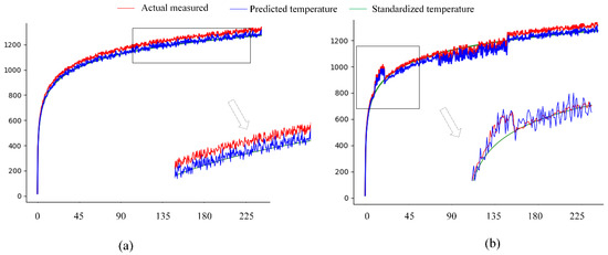
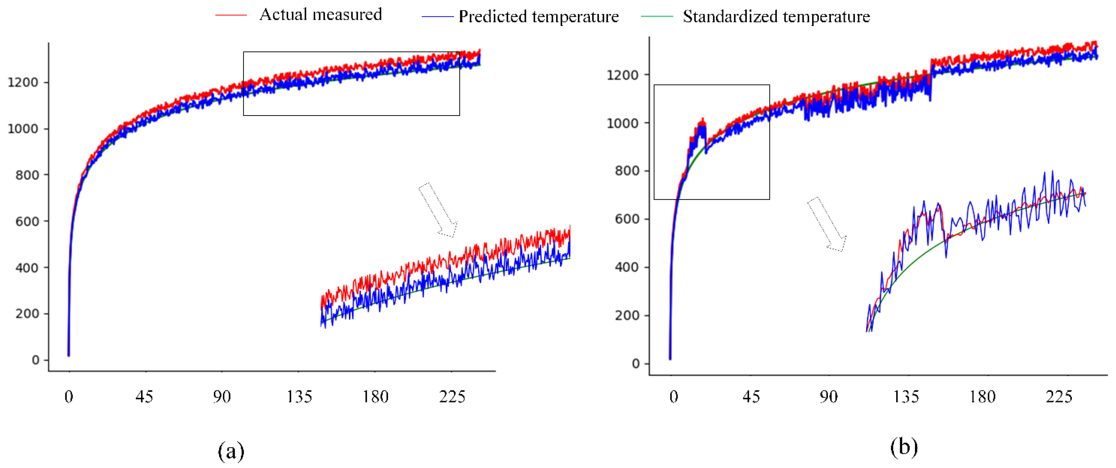
It is widely recognized that a high-accuracy prediction model for a target generally serves as a prerequisite for the control process. To this end, the prediction accuracy of the temperature prediction model is compared and evaluated in this section. In general, this comparison is conducted in two different forms in a normal process with little abnormal interruptions. To further demonstrate the effectiveness and robustness of the proposed method, temperature variations with interruptions are compared. The temperature variation curves for these two application scenarios are presented in Figure 7.

Figure 7. Measured and predicted temperature responses under normal and interruption conditions.

The figure is composed of two parts, and Figure 7a,b present the normal and abnormal situations with interruptions, respectively. In this figure, the red and blue lines denote the actual measured temperature variation and the predicted line, respectively. The green line in this figure denotes the standardized temperature variation line given by ISO 834. As shown in the figure, the red and blue temperature lines have the same variation trend, indicating that the proposed method can keep pace with the actual temperature. The same trend variation indicates that the effectiveness of the proposed method can be employed in the actual prediction stage. By comparing the blue or red temperature line with the green line, it can be observed that there is a slight difference, indicating that the actual temperature line is not accompanied by the desired one. The variation in these two lines further indicates the necessity of conducting an adaptive temperature control process. In particular, the difference between the blue, red, and green lines is shown in Figure 7, which further indicates that the temperature was interrupted owing to accidents. This variation further implies the necessity of employing an adaptive control method to modify the temperature line to the desired value.

To further demonstrate the effectiveness of the proposed method, a statistical analysis of the proposed method is presented in this section. Table 3 lists the corresponding statistical results and summarizes the prediction performance of the AMCNN model under normal and interruption conditions. Under normal operating conditions, the model achieves an MAE of 32.24 °C, an RMSE of 33.52 °C, and an R² of 0.953. Under interruption conditions, the MAE and RMSE increase to 41.03 °C and 47.50 °C, respectively, while R² decreases to 0.919. These results indicate that unexpected thermal disturbances increase the prediction error, although the model still preserves a relatively strong correlation with the measured temperature response.

Table 3. Prediction performance under normal and interruption conditions (MAE and RMSE in °C; R² dimensionless).

Metrics	MAE	RMSE	R2
Normal situation	32.24	33.52	0.953
With interruptions	41.03	47.50	0.919

This section verifies the effectiveness of the proposed method in terms of prediction accuracy. The results presented in the previous sections indicate that the proposed method can be employed to predict the combustion temperature, which provides evidence for controlling the process.

4.3. Comparison of Closed-Loop Control Performance

A further study was conducted to demonstrate the advantages of the proposed method in the control stage. Considering that the investigated furnace is a multi-channel coupled thermal system, additional baseline methods were introduced, including multi-variable PID, fuzzy PID, model predictive control (MPC), NSGA-II-based heat allocation, DRL without NSGA-III heat assignment, and the proposed method without the attention module. These methods cover conventional feedback control, adaptive control, optimization-based allocation, and learning-based control strategies. All controllers were tuned using the same training and validation datasets, and their parameters were optimized according to minimum temperature tracking error and thermal non-uniformity.

The parameter settings of the comparative methods are summarized as follows. PID used Kp = 0.85, Ki = 0.012, and Kd = 0.18 based on Ziegler–Nichols initialization and validation adjustment. Multi-variable PID adopted an 8 × 8 decoupling matrix with the proportional gain matrix adjusted to 0.72 and integral time of 85 s. Fuzzy PID used seven fuzzy subsets for error and error variation, with adaptive gain scaling factors of 0.8 and 1.2. MPC employed a prediction horizon of 20 steps, control horizon of 5 steps, and quadratic weighting factors of Q = 10 and R = 0.1. NSGA-II allocation used population size 100 and 200 generations to optimize heat distribution among channels. DRL without NSGA-III used the same DQN structure as the proposed controller but directly generated actuator commands without heat assignment. The proposed method without attention removed the attention module from the AMCNN while keeping other components unchanged. To provide a quantitative evaluation of various adaptive control methods, a statistical analysis using the MAE, R², and RMSE is presented in this report. The corresponding statistical results are shown in Table 4.

Table 4. Closed-loop control performance of different thermal regulation strategies (MAE and RMSE in °C; R² dimensionless).

Methods	MAE (°C)	RMSE (°C)	R2
Proposed method	19.90	24.70	0.9745
PID	32.86	40.28	0.9350
Multivariable PID	28.74	35.61	0.9472
Fuzzy PID	26.93	33.85	0.9521
MPC	24.85	31.20	0.9584
NSGA-II allocation + PID	23.71	29.96	0.9627
DRL without NSGA-III	25.42	32.14	0.9563
Proposed w/o attention	22.36	27.91	0.9681
No control	78.52	92.36	0.8125

As presented in Table 4, the proposed method achieves the lowest MAE and RMSE and the highest R² among all compared strategies. The comparison with multi-variable PID, fuzzy PID, MPC, and NSGA-II-based allocation demonstrates that the proposed hierarchical framework can better handle nonlinear coupling among multiple heating channels. The comparison with DRL without NSGA-III confirms the importance of the heat assignment layer, while the comparison with the proposed method without the attention module verifies the contribution of attention-based thermal feature extraction.

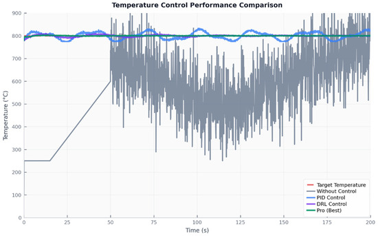
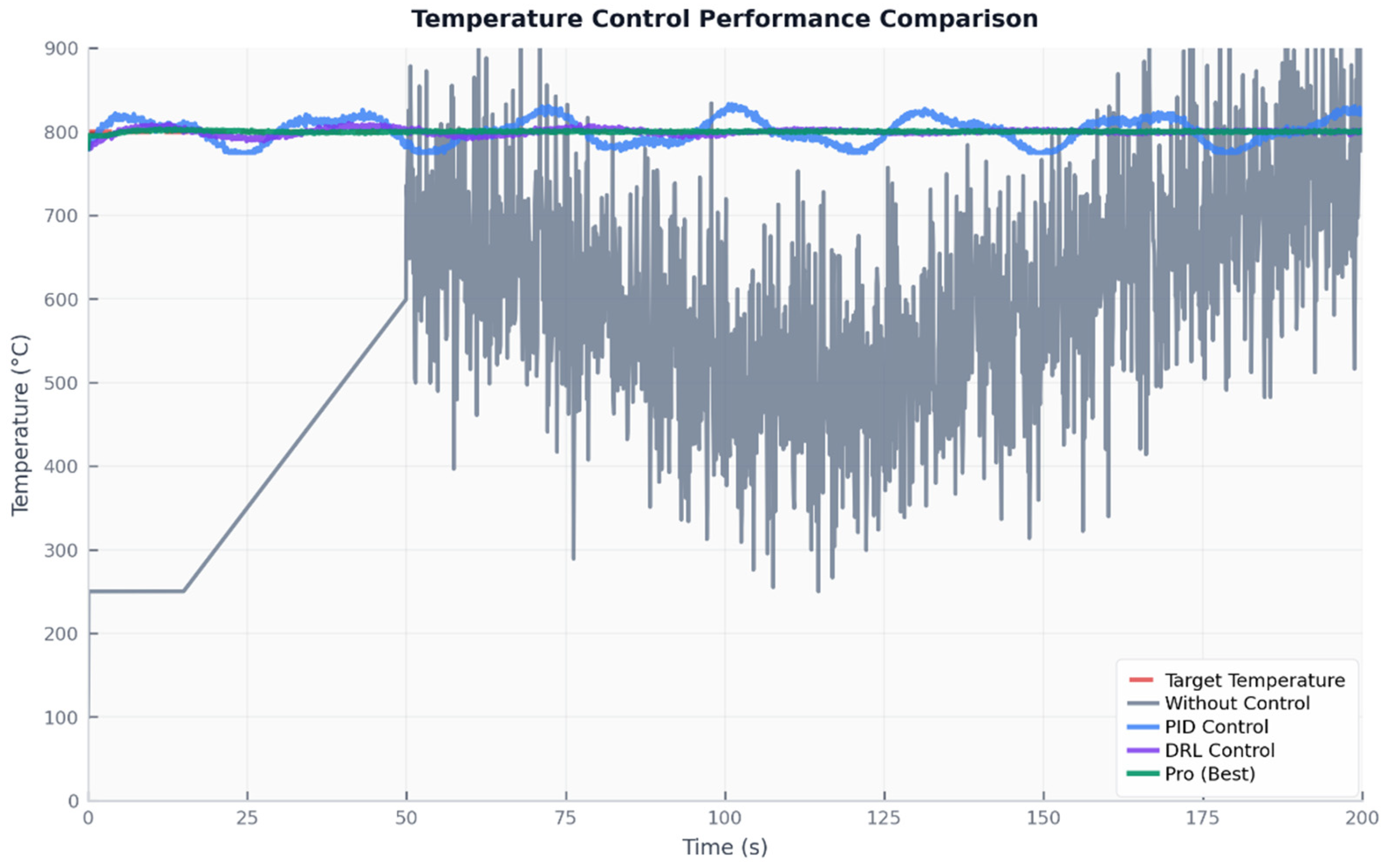
A further study has been employed to depict the effectiveness of the proposed method. The target temperature is set as 800 degrees, and multiple different methods have been employed and compared to depict the effectiveness. Results are given in Figure 8, which presents a comparative analysis of different control strategies for regulating combustion temperature in a dynamic system. The motivation for this comparison is to objectively evaluate the effectiveness of advanced control methods against traditional approaches and uncontrolled scenarios, which is crucial for ensuring safety, efficiency, and stability in industrial combustion processes. The plot displays the temperature response over time for four cases:

Figure 8. Closed-loop temperature responses of the compared control strategies.

• Without Control (gray): The system exhibits slow response and large fluctuations, failing to reach and maintain the target temperature reliably.
• PID Control (blue): The classic proportional-integral-derivative controller accelerates the response but introduces oscillations around the setpoint, indicating limited stability.
• DRL Control (purple): Deep reinforcement learning achieves faster convergence and improved stability compared to PID, with reduced oscillations and quicker attainment of the target.
• Proposed method (green): The proposed method demonstrates the fastest and most stable regulation, with minimal overshoot and the smallest fluctuations, closely tracking the target temperature throughout the process.

As mentioned in the previous sections, the second key point for controlling the combustion temperature is to help realize high thermal uniformity. Therefore, the performance of the proposed method and methods used to control thermal uniformity are discussed in this section. For this evaluation, all 32 fixed thermocouples were used to calculate the spatial thermal-uniformity metric, and the method for evaluating this parameter follows:

$$\mathrm{T}\mathrm{U}={\displaystyle \frac{{\sum }_{i=1}^{32}\mid y_{mea}^i-y_{average}\mid }{y_{average}\ast 32}}\ast 100\%$$

where $y_{average}$ denotes the average value of the measured combustion temperature, and $y_{mea}^i$ denotes the measured combustion temperature value of the $i$-th thermocouple. Because the combustion temperature varies with time, ten predefined, equally spaced evaluation stages covering the complete test duration are reported in Table 5 for a compact comparison. The metric at each stage is calculated from all 32 thermocouples and is expressed as a percentage. Additional summary statistics are calculated from all valid 10 Hz measurements rather than only these ten stages. Table 5 shows that the proposed method has a maximum normalized spatial deviation of 8.44%, compared with 18.20% for PID and 15.33% for DRL. The value 6.77% corresponds only to the fourth evaluation stage and is not the maximum deviation of the proposed method.

Table 5. Normalized spatial temperature deviation at ten predefined evaluation stages (%).

Time_Stage	1	2	3	4	5
Pro	3.94	2.22	3.11	6.77	1.80
PID	9.11	18.20	14.13	17.77	16.55
DRL	8.74	15.33	4.99	5.22	14.12
Time_stage	6	7	8	9	10
Pro	8.44	4.22	8.23	4.90	5.67
PID	14.33	13.44	11.20	15.36	10.43
DRL	10.41	12.22	10.10	5.78	9.11

In conclusion, the proposed method achieved significant success in controlling the combustion temperature. The proposed method not only improves thermal consistency but also the thermal uniformity, which can help control the combustion temperature in a more scientific manner. Compared with conventional methods, the proposed method is more applicable for controlling the combustion temperature in actual fire-resistance testing equipment, and offers a more scientific approach to improving the temperature variation during the actual test.

4.4. System Implementation and Online Computational Efficiency

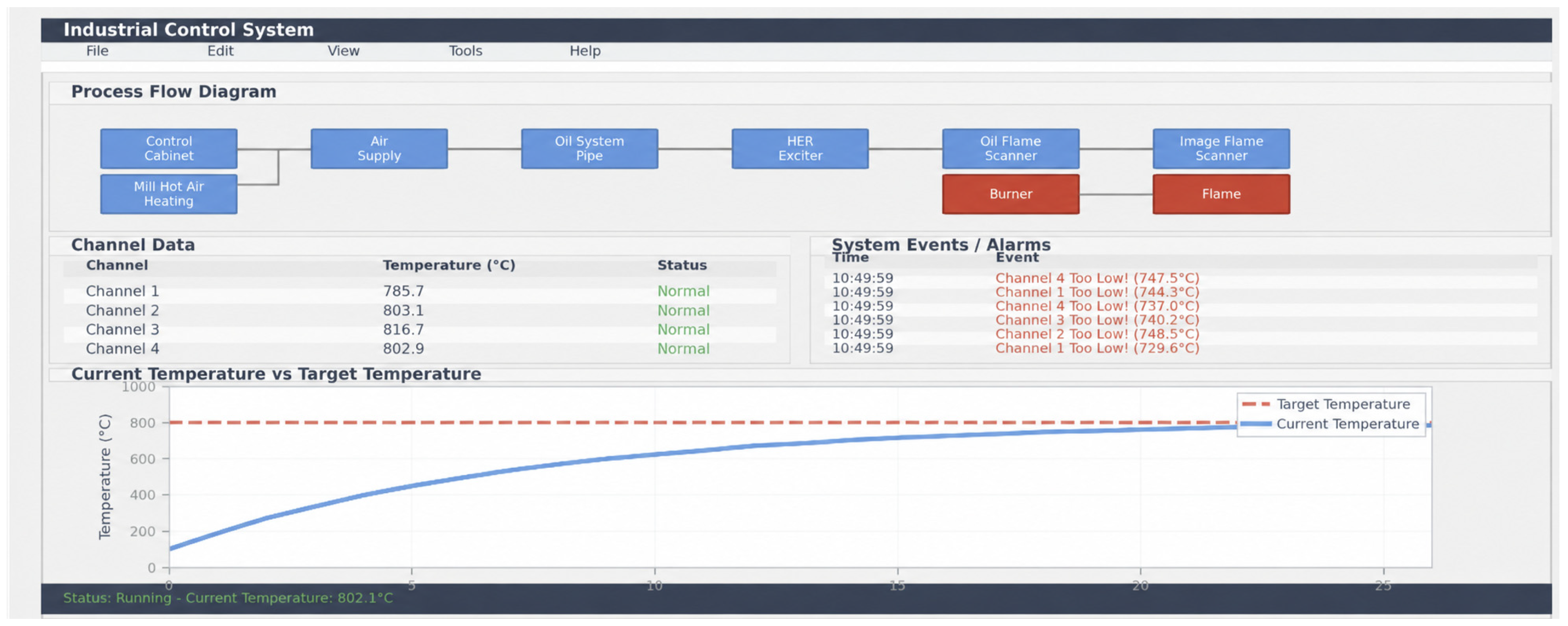
To demonstrate the effectiveness and practicality of the proposed method, this study developed a dedicated control system that has been successfully implemented in actual production lines. As shown in Figure 9, the system interface provides real-time visualization of dynamic changes in process parameters. The system employs an eight-channel collaborative control architecture for precise temperature monitoring and coordinated temperature adjustment across multiple channels during combustion.

Figure 9. Temperature control system.

The system provides two complementary feedback interfaces: a numerical view displays the temperature and command of each heating channel, while a graphical view presents the mean measured temperature, the AMCNN prediction, and the ISO 834 target curve. The complete NSGA-III–TOPSIS–DQN supervisory cycle is executed every 5 s, consistent with the slow thermal dynamics of the furnace.

The earlier ±1.5 °C statement described only short-term interface fluctuations and is not used as a full-process performance claim. Closed-loop performance is therefore reported consistently using MAE, RMSE, R², and the spatial thermal-uniformity metric.

To further illustrate the computational efficiency of the proposed method, ten independent end-to-end timing tests were conducted using the reported hardware and software platform. The recorded time covered data preprocessing, AMCNN inference, NSGA-III optimization, TOPSIS selection, DQN inference, command transmission, and actuator command update. Because the deployed system recorded only the total control-cycle time, the individual components were not timed separately. The furnace thermal settling time was not included in the reported computational latency. Although the sensor and process signals are acquired at 10 Hz, the supervisory optimization-control procedure is triggered at 5 s intervals. The timing measurement covers preprocessing, AMCNN inference, NSGA-III optimization, TOPSIS selection, DQN inference, command transmission, and actuator-command update; furnace thermal settling time is excluded.

As shown in Table 6, the end-to-end control-cycle time ranged from 3.68 to 4.47 s, with an average of 4.02 s and a standard deviation of 0.26 s. All ten tests were completed within the predefined 5 s supervisory control interval. These results demonstrate that the proposed method can satisfy the online decision-making requirement of the investigated furnace thermal-regulation process.

Table 6. End-to-end control-cycle timing results.

Test No.	Control-Cycle Time (s)	Control Deadline (s)	Satisfied
1	3.83	5	Yes
2	4.02	5	Yes
3	3.68	5	Yes
4	4.21	5	Yes
5	3.95	5	Yes
6	4.38	5	Yes
7	3.76	5	Yes
8	4.09	5	Yes
9	4.47	5	Yes
10	3.87	5	Yes
Average	4.02	5	Yes
Minimum	3.68	5	Yes
Maximum	4.47	5	Yes
Standard deviation	0.26	–	–

5. Conclusions

Ensuring the reliable operation of cables under fire scenarios is of great importance in modern society, as it can significantly reduce potential casualties and economic losses. Therefore, objective evaluation of cable fire-resistance performance is essential. Various testing methods and specialized equipment have been developed to assess fire-resistance capability. However, during conventional combustion tests, insufficient attention has been focused on thermal uniformity, although it directly influences the reliability and accuracy of evaluation results. Therefore, an intelligent adaptive thermal regulation method for fire-resistance testing equipment is proposed in this study.

The proposed method consists of three main steps, including thermal computational modeling, multi-channel optimization, and adaptive control. First, a nonlinear mapping relationship between heating flow inputs and combustion temperature responses is established using an attention-based multi-channel convolutional neural network, providing an effective computational model for predicting thermal responses under different operating conditions. Subsequently, a data-driven NSGA-III optimization strategy is employed to achieve real-time multi-objective optimization of multiple heating sources. Through this process, the optimal adjustment values of different heating channels can be obtained, and the coupling effects among multiple heat sources can be coordinated. Finally, a deep reinforcement learning-based adaptive controller is developed to achieve dynamic regulation of individual heating sources and maintain stable thermal conditions during the testing process.

Experiments were conducted using practical fire-resistance testing equipment to evaluate both the thermal prediction model and the closed-loop control framework. For thermal prediction, the AMCNN achieved an R² of 0.953 under normal operating conditions and an R² of 0.919 under interruption conditions, demonstrating its capability to capture the thermal response under different operating scenarios. For closed-loop thermal regulation, the proposed framework achieved an MAE of 19.90 °C, an RMSE of 24.70 °C, and an R² of 0.9745, outperforming the comparison control strategies. In addition, the proposed method provided improved spatial thermal uniformity, demonstrating its capability to simultaneously regulate temperature consistency and spatial temperature distribution.

Although the proposed method achieves significant improvements in thermal uniformity and consistency, the computational burden remains relatively high during practical implementation. Future studies will focus on developing lightweight computational models and efficient optimization strategies to accelerate real-time thermal regulation and improve deployment efficiency in fire-resistance testing systems.

References

- Kotsovinos, P.; Judge, R.; Walker, G.; Woodburn, P. Fire performance of structural cables: Current understanding, knowledge gaps, and proposed research agenda. J. Struct. Eng. 2020, 146, 03120002. [Google Scholar] [CrossRef] [Scilit]
- Han, L.-H.; Yang, Y.-F.; Yang, H.; Huo, J.-S. Residual strength of concrete-filled RHS columns after exposure to the ISO-834 standard fire. Thin-Walled Struct. 2002, 40, 991–1012. [Google Scholar] [CrossRef] [Scilit]
- Yang, D.; Liu, F.; Huang, S.-S.; Yang, H. ISO 834 standard fire test and mechanism analysis of square tubed-reinforced-concrete columns. J. Constr. Steel Res. 2020, 175, 106316. [Google Scholar] [CrossRef] [Scilit]
- Chaturvedi, S.; Vedrtnam, A.; Youssef, M.A.; Palou, M.T.; Barluenga, G.; Kalauni, K. Fire-resistance testing procedures for construction elements—A Review. Fire 2022, 6, 5. [Google Scholar] [CrossRef] [Scilit]
- Law, A.; Bisby, L. The rise and rise of fire resistance. Fire Saf. J. 2020, 116, 103188. [Google Scholar] [CrossRef] [Scilit]
- Kerekes, Z.; Restás, Á.; Lublóy, É. The effects causing the burning of plastic coatings of fire-resistant cables and its consequences. J. Therm. Anal. Calorim. 2020, 139, 775–787. [Google Scholar] [CrossRef] [Scilit]
- Madyaratri, E.W.; Ridho, M.R.; Aristri, M.A.; Lubis, M.A.R.; Iswanto, A.H.; Nawawi, D.S.; Antov, P.; Kristak, L.; Majlingová, A.; Fatriasari, W. Recent Advances in the Development of Fire-Resistant Biocomposites—A Review. Polymers 2022, 14, 362. [Google Scholar] [CrossRef] [Scilit]
- Liu, H.; Wang, W.; Yan, L.; Xu, Z. Combustion characteristic evolution and degradation mechanism of finished fire-resistant cables exposed to different ageing conditions. Process Saf. Environ. Prot. 2025, 197, 107011. [Google Scholar] [CrossRef] [Scilit]
- Yang, H.; Zhu, M.; Meng, F. Behavior of hot-cast anchor sockets for prestressed cable structures under fire. Structures 2023, 50, 1–9. [Google Scholar] [CrossRef] [Scilit]
- Zhou, C.; Cao, Z.; Wei, G.; Wu, K. Research on pyrolysis characteristics of pe outer sheath of high-voltage cables based on the principle of oxygen consumption. J. Electr. Eng. Technol. 2023, 18, 679–685. [Google Scholar] [CrossRef] [Scilit]
- Hong, Y.; Kang, J.; Fu, C. Tunnel fire smoke control based on the PID method: A numerical study. Tunn. Undergr. Space Technol. 2022, 124, 104450. [Google Scholar] [CrossRef] [Scilit]
- Feliu-Batlle, V.; Rivas-Perez, R. Design of a robust fractional order controller for burning zone temperature control in an industrial cement rotary kiln. IFAC-PapersOnLine 2020, 53, 3657–3662. [Google Scholar] [CrossRef] [Scilit]
- Zheng, F.; Lu, Y.; Fu, S. Research on temperature control of heating furnace with intelligent proportional integral derivate control algorithm. Therm. Sci. 2020, 24, 3069–3077. [Google Scholar] [CrossRef] [Scilit]
- Jamil, A.A.; Tu, W.F.; Ali, S.W.; Terriche, Y.; Guerrero, J.M. Fractional-order PID controllers for temperature control: A review. Energies 2022, 15, 3800. [Google Scholar] [CrossRef] [Scilit]
- Borase, R.P.; Maghade, D.K.; Sondkar, S.Y.; Pawar, S.N. A review of PID control, tuning methods and applications. Int. J. Dyn. Control 2021, 9, 818–827. [Google Scholar] [CrossRef] [Scilit]
- Li, Z. Review of PID control design and tuning methods. J. Phys. Conf. Ser. 2023, 2649, 012009. [Google Scholar] [CrossRef] [Scilit]
- Gao, L.; Yang, Y.; Ren, X.; Gu, H.; Han, Q.; Yu, J. College of Electrical Engineering, Nantong University, Jiangsu Nantong Research on Temperature Control System Based on IPSO Optimized Fuzzy PID. In Proceedings of the 2020 39th Chinese Control Conference (CCC), Shenyang, China, 27–29 July 2020. [Google Scholar]
- Lissa, P.; Deane, C.; Schukat, M.; Seri, F.; Keane, M.; Barrett, E. Deep reinforcement learning for home energy management system control. Energy AI 2021, 3, 100043. [Google Scholar] [CrossRef] [Scilit]
- Yu, L.; Sun, Y.; Xu, Z.; Shen, C.; Yue, D.; Jiang, T.; Guan, X. Multi-agent deep reinforcement learning for HVAC control in commercial buildings. IEEE Trans. Smart Grid 2020, 12, 407–419. [Google Scholar] [CrossRef] [Scilit]
- Yu, L.; Qin, S.; Zhang, M.; Shen, C.; Jiang, T.; Guan, X. A review of deep reinforcement learning for smart building energy management. IEEE Internet Things J. 2021, 8, 12046–12063. [Google Scholar] [CrossRef] [Scilit]
- Brandi, S.; Piscitelli, M.S.; Martellacci, M.; Capozzoli, A. Deep reinforcement learning to optimise indoor temperature control and heating energy consumption in buildings. Energy Build. 2020, 224, 110225. [Google Scholar] [CrossRef] [Scilit]
- Taboga, V.; Bellahsen, A.; Dagdougui, H. An enhanced adaptivity of reinforcement learning-based temperature control in Buildings using generalized training. IEEE Trans. Emerg. Top. Comput. Intell. 2021, 6, 255–266. [Google Scholar] [CrossRef] [Scilit]
- Wei, T.; Wang, Y.; Zhu, Q. Deep reinforcement learning for building HVAC control. In Proceedings of the DAC ‘17: The 54th Annual Design Automation Conference 2017, Austin, TX, USA, 18–22 June 2017. [Google Scholar]
- Liu, S.; Liu, Z. Multi-channel CNN-based object detection for enhanced situation awareness. arXiv 2017, arXiv:1712.00075. [Google Scholar]
- Wu, P.; He, Y.; Li, Y.; He, J.; Liu, X.; Wang, Y. Multi-objective optimisation of machining process parameters using deep learning-based data-driven genetic algorithm and TOPSIS. J. Manuf. Syst. 2022, 64, 40–52. [Google Scholar] [CrossRef] [Scilit]
- Liu, Z.; Huang, H.; Lu, C.; Lyu, S. Multichannel cnn with attention for text classification. arXiv 2020, arXiv:2006.16174. [Google Scholar]
- Wei, X.; Zhou, L.; Chen, Z.; Zhang, L.; Zhou, Y. Automatic seizure detection using three-dimensional CNN based on multi-channel EEG. BMC Med. Inform. Decis. Mak. 2018, 18, 71–80. [Google Scholar] [CrossRef] [Scilit]
- Wang, Y.; Huang, M.; Zhu, X.; Zhao, L. Attention-based LSTM for aspect-level sentiment classification. In Proceedings of the 2016 Conference on Empirical Methods in Natural Language Processing, Austin, TX, USA, 1–5 November 2016. [Google Scholar]
- Zhang, X.; Liang, X.; Zhiyuli, A.; Zhang, S.; Xu, R.; Wu, B. At-lstm: An attention-based lstm model for financial time series prediction. IOP Conf. Ser. Mater. Sci. Eng. 2019, 569, 052037. [Google Scholar] [CrossRef] [Scilit]
- Ishibuchi, H.; Imada, R.; Setoguchi, Y.; Nojima, Y. Performance comparison of NSGA-II and NSGA-III on various many-objective test problems. In Proceedings of the 2016 IEEE Congress on Evolutionary Computation (CEC), Vancouver, BC, Canada, 24–29 July 2016. [Google Scholar]
- Ciro, G.C.; Dugardin, F.; Yalaoui, F.; Kelly, R. A NSGA-II and NSGA-III comparison for solving an open shop scheduling problem with resource constraints. IFAC-PapersOnLine 2016, 49, 1272–1277. [Google Scholar] [CrossRef] [Scilit]
- Deb, K.; Jain, H. An evolutionary many-objective optimization algorithm using reference-point-based nondominated sorting approach, part I: Solving problems with box constraints. IEEE Trans. Evol. Comput. 2013, 18, 577–601. [Google Scholar] [CrossRef] [Scilit]
- Behzadian, M.; Otaghsara, S.K.; Yazdani, M.; Ignatius, J. A state-of the-art survey of TOPSIS applications. Expert Syst. Appl. 2012, 39, 13051–13069. [Google Scholar] [CrossRef] [Scilit]
- Li, Y. Deep reinforcement learning: An overview. arXiv 2017, arXiv:1701.07274. [Google Scholar]
- Vincent, F.L.; Peter, H.; Riashat, I.; Marc, G.B.; Joelle, P. An introduction to deep reinforcement learning. Found. Trends Mach. Learn. 2018, 11, 219–354. [Google Scholar] [CrossRef] [Scilit]
Disclaimer/Publisher’s Note: The statements, opinions and data contained in all publications are solely those of the individual author(s) and contributor(s) and not of MDPI and/or the editor(s). MDPI and/or the editor(s) disclaim responsibility for any injury to people or property resulting from any ideas, methods, instructions or products referred to in the content. |
© 2026 by the authors. Licensee MDPI, Basel, Switzerland. This article is an open access article distributed under the terms and conditions of the Creative Commons Attribution (CC BY) license.