


Abstract
Climate change poses several challenges for the economic system. The financial and insurance industries are called on to play a pivotal role, in particular in coming up with innovative solutions such as sustainable products. According to the EU’s Sustainable Finance Disclosure Regulation, sustainable products have to meet the requirement of pursuing a sustainable investment objective. Furthermore, they need to have measurable goals in place aligned with the investment objective, which can be reported to clients, in order to achieve an advanced understanding of the potential performance to obtain more effective stress scenario analysis. Accordingly, the design of insurance products requires suitable risk and profitability analytics. In our paper, we provide an innovative risk analytical tool for the design of sustainable insurance products environmentally linked, that is, a Climate Conditional Value at Risk (CCVaR), based on Random Forests with a Canonical Correlation Analysis algorithm, building a VaR of climate-related portfolio volatility that is obtained by assessing how the relationships between volatilities of portfolio assets modify according to the bioclimatic indicators. In particular, we propose a splitting rule for the Random Forest algorithm based on OVERALS, a generalisation of Canonical Correlation Analysis based on similarities and not on correlations, considering a more general perspective of non-linear relationships.
MSC:
91G15; 62R20; 68T05
1. Introduction
Sustainability has declined in the Environmental, Social, and Governance dimensions, coining the ESG term that has grown from a corporate social responsibility initiative launched by the United Nations (UN) into a global phenomenon. Accordingly, there is a broad consensus that businesses will have to pay more attention to the expectations of key stakeholders such as investors, regulators, policyholders, and employees towards the development of more sustainable versions of products and services offered by the market.
Sustainability represents a broad concept. Assessing product sustainability is a complex task. The actuaries and financial analysts are working to make positive contributions to sustainability, also by supporting the development of sustainable insurance products.
Particularly, “insurers are exploring the scope for generating additional social benefits from explicitly adopting ESG considerations in their core business activities” [1]. In this context, sustainable insurance products require not only the identification of their environmental and social objectives but also the assessment of the risks arising from climate change and their potential financial consequences [2]. Under the principle of double materiality [3], insurance companies should consider both the impact of their activities on ESG factors (inside-out perspective) and the effects of climate-related risks on their own financial and operational resilience (outside-in perspective). The latter perspective requires quantitative tools capable of measuring how climate conditions affect insurance and financial risks over time. The measurement of climate risk could grade the sustainability level of a financial or insurance product, such as, for instance, light green or dark green, already in the product design phase [4]. According to the Financial Stability Board, “a systemic event is a disruption to the flow of financial services that is caused by an impairment of all or parts of the financial system and has the potential to have serious negative consequences on the real economy” [5]. Climate-related risk can therefore be considered a systemic risk, as climate shocks may affect multiple sectors simultaneously and alter both insurance liabilities and financial market conditions.
In this paper, we propose a methodological framework to calculate a Climate Conditional Value at Risk (CCVaR), based on quantifying how climate-related factors affect the financial risk profile of portfolios and insurance products. The proposed approach does not only evaluate the potential losses associated with adverse climate conditions, but also accounts for the fact that climate variables may modify the dependence structure among financial and economic risk factors over time. By modelling the conditional evolution of portfolio risk as a function of climate and macroeconomic variables, CCVaR provides a dynamic measure that can support portfolio allocation, insurance product design, and climate stress testing.
Unlike traditional Climate VaR approaches, which are generally based on predefined climate scenarios and long-term projections, the proposed framework is data-driven and estimates how observed climate conditions influence the risk distribution of financial variables. This feature is particularly relevant for risk management purposes, since climate-related shocks may generate nonlinear effects and changes in dependence patterns that cannot be adequately captured by static correlation measures or scenario-based assessments alone. The Climate Value at Risk has already been implemented by several institutions. A report of Ninety One points out that 43% of surveyed asset owners already implement Climate Value at Risk, rising to 54% among Asia-Pacific firms [6]. Nevertheless, there exists no one way to build Climate Value at Risk. The robustness of a given measure of climatic risks has to be intrinsically related to their main characteristics: forward-looking nature, deep uncertainty, non-linearity, and endogeneity [7]. These characteristics imply that climate risk cannot be fully represented through static indicators or predefined scenarios only, since climate-related shocks may generate nonlinear effects and modify the dependence relationships among financial variables. Climate risks could lead to material risks for financial and insurance companies, which need to redefine the prudential risk conditions to take into account [8]. Limiting the analysis to physical risk only, an increase in the frequency and severity of weather events and natural catastrophes determines a higher number of claims for climate-related insurance contracts such as crop products, damaged property products, non-damage business interruption products, and so on. Furthermore, extreme events would impact the creditworthiness of firms and individuals, resulting in higher credit insurance claims. Climate risks also could lead to negative effects on the capital market, with higher credit spreads on government bonds of countries highly susceptible to physical risks, and also affect the financial system, depressing interest rates and asset values. Greater uncertainty in the capital market determines the need for more sources of hedging, with higher reinsurance and capital costs. From a practical perspective, CCVaR can support different categories of users in climate risk management. For portfolio managers, the proposed measure provides information on how climate conditions affect portfolio risk over time and can be used to compare alternative asset allocations under adverse climate scenarios. In particular, CCVaR allows identifying whether diversification benefits remain effective when climate-related shocks modify the dependence structure among assets.
For insurance companies, CCVaR can support several phases of the insurance product life cycle, including product design, pricing, underwriting, and capital management. For example, in climate-related insurance products, such as agricultural or property insurance, CCVaR can help evaluate how changes in physical risk indicators affect the volatility of underlying assets and the dependence between different risk components. This information can contribute to the definition of pricing assumptions, reinsurance strategies, and solvency assessments.
Furthermore, CCVaR can be used as a climate stress-testing framework. Under extreme climate scenarios, such as an increase in the frequency of heat waves, droughts, or catastrophic events, the model allows evaluating how portfolio risk changes when climate variables alter both volatility and dependence patterns. Broadly speaking, the definition of an environmentally sustainable product requires defining not only the prudential risks common for all insurance or financial products but also the potential impact of the climate risks on them. The assessment of climate financial risk requires modelling how climate variables influence both the volatility distribution of financial assets and the dependence structure among different risk factors. In this sense, we consider a tree-based algorithm that allows making short-term predictions on the distribution of returns to a series of covariates related to physical risk. The basic idea is that climate risks, physical or transitional, are strongly related to financial risks; we could measure them with climate-related asset volatility and then estimate a reliable model for financial climate risk. It is necessary to consider the relations between the covariates that define the climate risk. Several approaches in the field of tree-based algorithms with dependence among covariates are proposed. We focus our attention on the approaches based on canonical correlation analysis since we can consider climate risk as a series of multivariate blocks of risks, defined by a series of covariates. We develop a Random Forest (RF) based on the splitting rule that considers the non-linear canonical correlation projections using the OVERALS algorithm.
In particular, in the designing of predictive modelling of a climate-related insurance product, it is necessary to consider all the possible covariates that can affect it. For example, to make an accurate risk assessment for crop insurance, it is not enough to limit the analysis of the yield levels; it is necessary to assess the causes, such as weather events, land type, and energy supply. In addition, climate change changed the distribution and nature of adverse events, resulting in greater uncertainty in the assessment of risks related to weather events. On the basis of these considerations, the Random Forest with Canonical Correlation Analysis algorithm [9], which allows assessing how the relationships between blocks of variables change as a function of a series of covariates, is suitable for the risk evaluation of climate-related sectors in the function of bioclimatic indicators. However, both for the complexity of the relationships and for the nature of the variables considered, not necessarily continuous, the hypothesis of linearity of the relations subject to the Canonical Correlation Analysis is inadequate. Therefore, we propose a splitting rule based on the OVERALS algorithm [10] and a generalisation of Canonical Correlation Analysis based on similarities and not on correlations, considering a more general perspective of non-linear relationships.
It is also worth noting that many of the existing climate VaR measures are long-term projections, while VaR is a tool designed for short-term assessments. This leads to a distortion of the actual assessment of climate risk in finance, as the measures mainly refer to climate change over time horizons of decades or a century, when the effects of climate risk in financial markets are already present. In our approach, we address this limit by using a dynamic Climate VaR whose portfolio variance is modeled conditionally with respect to climate and economic variables. It is a short-term and data-driven projection.
The layout of the paper is the following. Section 2 provides an overview of the literature on climate risk management, climate-related metrics and the actuarial application of climate VaR; Section 3 presents the methodology, starting from the Climate CVaR, and then introducing the Dependent Forest Non-Linear Canonical Correlation DF-NLCC as an extension of the Random Forest with Canonical Correlation Analysis and its use for the estimation of the conditional dependence of a portfolio composed of blocks of climate-related sectors; Section 4 shows numerical results, comparing the use of RFCCA with economic-only conditioning variables or adding climate variables and comparing RFCCA with DF-NLCC, through the use of categorical variables representing the portfolio block regimes; finally, Section 5 concludes.
2. Literature Review
2.1. Climate Risk Management
Due to the incontrovertible systemic nature of the climate-related risk underlines the need for operational stress testing models. In response to this need the analytics, in particular in the asset management sector, has developed climate stress testing considerably in recent years, especially in the banking sector. Several stress testing models have been proposed by central bankers and academics, beyond the pioneering work [11], for instance this approach has been extended to investment funds [12] and widely recognised [13,14,15]. The main typical stress testing tools to address sustainable finance risk management, connecting climate change with financial risks focus on the tails of a distribution of losses based on Value-at-Risk (VaR) models [16]. The earliest approaches to assess the impact of climate change on the value of financial assets has been developed [17]. Another interesting climate risk management tool has been introduced by the Federal Reserve Bank of New York, exclusively related to the impact of transition risks: the so called CRISK stress-testing procedure, which detects the expected capital shortfall of a financial institution by analysing the climate-related risk exposure of large banks. This is called climate-beta [18]. Nevertheless, as suggested [19] Conditional-VaR represents a measure of alternative risk that is preferred to the common VaR concept, since it tends to satisfy the four properties of a coherent risk measure, i.e., translation invariance, monotonicity, subadditivity and positive homogeneity [20] and it is an estimate of the size of the tail loss, which gives a more accurate estimate of the associated risk [21].
2.2. Measuring Climate-Related Financial Risk
The relationship between climate and financial risks is a topic of great interest in the academic literature [11,12,22,23,24,25], in the financial community [26,27], and among practitioners [28].
The exposure of companies to the negative effects of greenhouse gas emissions affects not only the economic sector but also the financial system and destabilises it. For this reason, it is necessary to define measures to determine the dependency between financial risks and climate risks. In particular, the value of an undertaking or sector exposed to climate risk is susceptible to revaluation in the financial market, and these revaluations depend on both transition risks and physical risks. The instability of the sustainability market is mainly caused by the huge number of transactions in the field of green finance and ESG, given the increasing interest in the issue. As a consequence, firm and sector exposures are susceptible to potentially large financial market repricing [29].
The effects on financial markets of climate risks should be considered as any other financial risk and accurately assessed, monitored, and controlled [30]. It is also important to define a regulatory framework to operate [29]. As well as ESG investments presenting heterogeneity to be modelled [31], it is possible to define climate-related risk metrics that combine all the possible risks in terms of evaluation. Part of the observed heterogeneity in risk assessments is associated with differences in the methodologies used by the different providers. The heterogeneity in risk assessments reflects the significant complexity and uncertainty in the analysis of climate risks.
Based on the methodology, we can distinguish among score metrics, which give a score to undertakings that may be related either to the impact of emissions in the exercise of firms’ economic activity, e.g., Carbone4 Overall rating [32], or to the effects on the economic activity of emissions, e.g., ClimateWise Transition risk score [33]; climate-related metrics, carrying out a risk assessment based on scenario analysis considering the achievement of particular emission targets or time horizons, e.g., MSCI Climate VaR [34]; management metrics, that assess the sensitivity and ability of companies to adapt to a climate-friendly vision, e.g., S&P Global ESG Scores [35]. In particular, among the main climate-related metrics, we can find the following shown in Table 1.
Table 1.
Climate-related metrics.
Ref. [36] proposes a comparison of 12 financial climate-risk-based metrics considering 287 firms from 10 sectors. The comparison is performed in two ways: across-metrics and within-metrics analysis. The across-metrics analysis investigates if the metrics determine different results in terms of the sensitivity of a firm or a sector to climate risk, while the within-metrics analysis assesses the differences in results produced by the same metric considering different transition scenarios in terms of temperature targets and time horizons.
Metrics show heterogeneity in terms of scores and sensitivity to climate scenarios and time horizons. It reflects the fact that risk metrics differ in terms of the methodology adopted and the assumptions made, as well as the data inputs used. However, most and least exposed companies to climate risks show similar results for all the metrics, and the results are more similar if the metrics are based on the same methodologies.
2.3. Actuarial Application of Climate Conditional VaR
This paper proposes a comprehensive climate stress testing approach to measure the impact of the climate risk in the modelling of a climate-related insurance product related to Product Development and Innovation and also in the context of their own risk and solvency assessment (ORSA) or the development of their capital and their risk management policies for micro-prudential objectives. The other stakeholders (rating agencies and other institutions) also might implement CCVaR for analytical purposes. In other words, the stress testing based on Climate Conditional VaR we propose relies on the assessment of the resilience of the individual insurers to adverse scenarios, providing supervisors with information on whether these insurers are able to withstand severe shocks and take remedial action if necessary. In the macroprudential perspective, the adapted CCVaR tool we provide can contribute to detecting the resilience of the insurance industry as a whole, by addressing the systemic climate risk and potential spillovers to the real-economy. After all, the Conditional Value-at-Risk is included in a suite of popular and statistically robust tools applied in the financial sector based on the well-established statistical theories.
3. Methodology
3.1. Climate Conditional Value at Risk
Climate VaR is a methodology proposed by [17]. It consists of a new measure to assess the potential financial losses due to climate change for a company or an asset portfolio. While following the logic of VaR, it specifically analyses risks and opportunities arising from climate change. Climate VaR is an important tool to address companies making investment choices that reduce their exposure to climate risks.
Ref. [34] proposed a version of Climate VaR allowing the determination of the climate financial risks, considering a series of theoretical scenarios about policy, transition, and physical risks. The policy risk measure is based on the country’s greenhouse gas (GHG) emission reduction targets defined in the Paris Agreement, based on the economic sector, and the future carbon prices, to calculate the cost of the emissions reduction targets by sector. The transition risk measure assesses the impact of green revenue market shares and the use of low-carbon technologies based on patents, evaluated according to patent citations, geographic area, and sector coverage. The physical risk measure assesses the possible scenarios resulting from increased levels of GHG emissions and their costs on business activities. The three risk profiles are calculated as a percentage of the market value of the equity’s market values, considering different level thresholds for various degrees of severity. The VaR is calculated on the sum of the three risk profiles.
This Climate Value-at-Risk [34] provides a forward-looking and return-based valuation assessment to measure climate-related risks and opportunities in an investment portfolio. However, it has some limitations to be filled. The first limit is linked to the definition of Value at Risk (VaR). As noted in literature [37], value at risk fails as a consistent measure of risk. The axioms of consistency are indispensable mathematical tools for an unbiased assessment of risk, so it is important to refer to a measure that respects all of them. In particular, a risk measure is a function , where V is a set of real-valued random variables, that satisfies the following conditions: In particular, a risk measure is a function , where V is a set of real-valued random variables, that satisfies the following conditions.
VaR does not satisfy the condition of sub-additivity. As pointed out by [38], the condition of sub-additivity is the basis of the risk diversification strategy; that is, the possible sources of risk do not have the same effect on all components of the portfolio, leading to a total risk at most equal to the sum of the individual risks. A measure that does not respect the condition of sub-additivity may lead to the paradox of a total risk greater than the sum of the individual risks. This result is unrealistic not only in the area of portfolio optimisation but also in the field of capital adequacy requirements.
The recent literature has further investigated the statistical properties of Expected Shortfall and the problem of its empirical validation. In particular, ref. [39] analysed the elicitability properties of risk measures, showing the importance of considering joint estimation and backtesting procedures for Value-at-Risk and Expected Shortfall. Moreover, ref. [40] proposed backtesting approaches specifically designed for Expected Shortfall, highlighting the need for statistically consistent validation procedures when this measure is adopted in financial risk management. In regulatory applications, Expected Shortfall has also replaced Value-at-Risk as the reference market risk measure within the Basel III/FRTB framework [41]. Furthermore, concerning the Climate VaR proposed by [34], it should be noted that it refers to long-term projections based on scenario analysis relating to temperature rise on temporal horizons of about a century, while the VaR is generally used for short-term forecasts and uses stochastic modelling.
This distinction is particularly relevant because financial risk measures require models capable of adapting to changing market conditions and incorporating nonlinear interactions among risk drivers. Recent developments in financial econometrics have shown the potential of machine learning (ML) approaches for forecasting, as they can capture complex patterns and nonlinear relationships that may not be adequately represented by traditional parametric models [42,43]. For these reasons, we propose a risk measure based on Conditional VaR (CVaR), obtained from out-of-sample forecasts of climate-related portfolio conditional dependence based on a RF algorithm with a specific splitting rule based on non-linear canonical correlations. It is shown that CVaR is a sub-additive measure, and it is usable in cases of high dimensionality [44].
The assessment of climate financial risk concerns the estimation of the distribution of asset as a function of climatic adverse events. In this sense, we consider a tree-based ML algorithm that allows making short-term predictions on the distribution of returns to a series of covariates related to physical risk. The basic idea is that climate risks, physical or transitional, affect financial risks, and we can estimate a model that measures the climate-related assets volatilities to obtain a reliable model to estimate climate-related financial risk.
Therefore, the proposed framework combines recent developments in ML-based forecasting with climate risk modelling, allowing the conditional distribution of portfolio losses to evolve according to observed climate and economic conditions.
3.2. Dependent Forest Non-Linear Canonical Correlation (DF-NLCC)
Several approaches in the field of tree-based algorithms with dependence among covariates are proposed. RF algorithms introduced by [45] are designed to construct recursive partitions of the predictor space according to the heterogeneity of a response variable. However, in multivariate risk applications, the objective may be not only the prediction of a response but also the identification of changes in dependence structures among groups of variables. The Random Forest with Canonical Correlation Analysis (RFCCA) framework proposed by [9] extends this idea by partitioning the conditioning variable space according to variations in the canonical dependence between two multivariate blocks. It is worth noting that modelling the dependence structure among financial variables has been extensively studied in financial econometrics. In particular, Dynamic Conditional Correlation (DCC) models [46] represent one of the most widely adopted approaches for describing time-varying dependence through parametric multivariate volatility models. More recently, ML approaches have also been proposed to model volatility and dependence in a more flexible and data-driven framework [47]. However, these approaches are generally aimed at modelling the temporal evolution of covariance or volatility processes rather than identifying regions of the covariate space characterised by heterogeneous dependence structures.
Formally, let a sample of N observational units and two multivariate blocks and . Canonical Correlation Analysis (CCA), introduced by [48], determines linear combinations of and that have a maximum correlation with each other. In particular, CCA finds the vectors and that maximise the correlation between and .
Following [9], the vector denotes a set of static conditioning variables associated with the i-th observational unit. Therefore,
The objective is to identify regions of the conditioning variable space where the dependence structure between the two multivariate processes changes. Following the conditional canonical correlation framework, a recursive partitioning algorithm is used to construct nodes according to the conditioning variables . For a generic node , the RFCCA conditional canonical correlation is defined as
where and denote the observations assigned to node . A candidate split divides node into two child nodes and , and the RFCCA splitting criterion is defined as
This criterion identifies partitions of the conditioning space characterised by heterogeneous linear dependence structures. Specifically, for a generic node ,
denotes the set of observational units assigned to that node. The dependence between and is evaluated locally within each node, and candidate splits are selected according to the heterogeneity of the resulting dependence measures. We develop a Dependent Forest based on Non-Linear Canonical Correlation estimation with random forests (DF-NLCC), as an extension of RFCCA. This method allows estimating the non-linear canonical correlations, based on similarity measures, between two sets of variables, depending on a set of subject-related covariates.
The RFCCA approach considers only linear relationships that, in the perspective of the implementation of ML algorithms, appear limited for the data complexity considered. The splitting rule we propose considers the non-linear canonical correlations projections using the OVERALS algorithm [10], preserving the main difference between RFCCA and the RF, that is, the splitting rule is determined through the selection of the latent variables obtained in the projected canonical space, obtained by performing the analysis of the canonical correlations on all the covariates considered.
For each node , let denote the two multivariate blocks of limited dependent variables assigned to the node. The objective of OVERALS is to identify the common structure between the two sets by estimating latent object scores and weights that make the weighted combinations of the sets as similar as possible. The classical multi-set canonical correlation formulation can be expressed as
where represents the j-th block of variables, u denotes the vector of object scores and represents the weights associated with the variables of the j-th set. The nonlinear extension introduced by OVERALS is obtained through optimal scaling. Specifically, the original data blocks are replaced by optimally transformed blocks , whose columns satisfy the measurement restrictions associated with the observed variables. Therefore, the OVERALS model is formulated as
subject to the orthogonality constraints among extracted dimensions and , where denotes the matrix of latent object scores and defines the admissible class of transformations for variable t. (e.g., numerical, ordinal, or nominal). The optimal transformations and provide a nonlinear representation of the original blocks while preserving the common dependence structure between them. The node-specific nonlinear canonical dependence measure is then defined as
Therefore, the DF-NLCC splitting criterion is obtained by replacing the linear canonical correlation of RFCCA with the optimal-scaling-based dependence measure
The optimal split is selected as the partition maximising among all candidate variables and split points. Hence, DF-NLCC preserves the original RFCCA interpretation of conditional dependence estimation while allowing nonlinear dependence structures between and to be identified according to the conditioning block .
It is worthy to note that RFCCA and DF-NLCC coincide when all variables included in the and blocks are continuous. In this case, OVERALS reduces to a linear transformation of the original variables. Since CCA is invariant to nonsingular linear transformations of the variables within each block, the canonical correlations obtained from OVERALS coincide with those obtained from standard CCA. Consequently, the dependence measure used by DF-NLCC is equivalent to that used by RFCCA, and the two procedures yield the same results when and contain only continuous variables.
In the DF-NLCC algorithm, purity is not defined in terms of the homogeneity of a response variable, as in standard RF, but in terms of the homogeneity of the conditional dependence structure. A terminal node is therefore considered homogeneous when the nonlinear canonical dependence measure estimated within the node is approximately constant across the observations assigned to that region.
The splitting criterion aims to identify intermediate nodes where the dependence structure changes significantly After recursive partitioning, the terminal nodes represent regions of the conditioning space where the dependence structure between the two multivariate blocks is expected to be more stable Thus, the proposed splitting criterion provides a dependence-based analogue of impurity reduction in classical RF methods. The criterion does not imply a global optimisation of the dependence structure, since the tree construction remains a greedy recursive procedure, but it provides a theoretically motivated local criterion for detecting heterogeneous dependence regimes.
Furthermore, DF-NLCC present a main additional computational cost with respect to RFCCA due to the estimation of the nonlinear canonical dependence through the iterative OVERALS optimal scaling procedure. For each candidate split, the algorithm requires the construction of the two child nodes; the optimal scaling transformation of the variables; the estimation of the nonlinear canonical dependence measure.
Let denote the number of observations in node , the total number of variables in the two multivariate blocks, d the number of extracted dimensions, and s the number of iterations required by the ALS optimisation. The computational cost of the OVERALS step is approximately
for each candidate split. Therefore, the overall complexity of DF-NLCC is higher than RFCCA because the standard CCA estimation is replaced by an iterative nonlinear optimisation procedure.
Regarding convergence properties, the OVERALS optimisation is based on an ALS procedure. At each iteration, the optimisation updates one set of parameters conditional on the remaining ones, leading to a non-increasing value of the loss function
Since the loss function is bounded below by zero, the optimisation sequence converges to a local optimum of the OVERALS objective function.
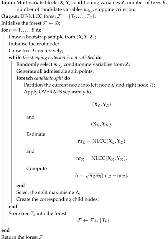
The tree-growing procedure follows the standard RF recursive partitioning mechanism. At each node, the candidate splits are evaluated according to , and the split producing the largest dependence heterogeneity is selected. The recursive procedure terminates according to standard stopping criteria, such as maximum tree depth or minimum node size.
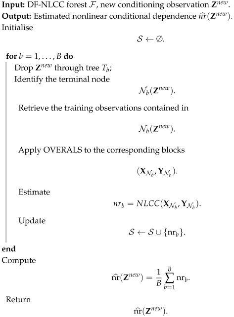
Algorithm 1 define the pseudo-code of the DF-NLCC estimation procedure and Algorithm 2 the non-linear dependence structure prediction using DF-NLCC.
| Algorithm 1: Estimation of the DF-NLCC. |
 |
| Algorithm 2: Prediction of DF-NLCC. |
 |
3.3. CCVaR Estimation Using DF-NLCC
Using the proposed framework, we define a time-varying Climate CVaR based on the conditional dependence structure estimated by DF-NLCC and on the resulting climate-dependent portfolio risk distribution. The considered portfolio is composed of climate-sensitive commodities belonging to different sectors, such as energy and agri-food, which exhibit significant co-movements in prices and volatility (e.g., [49,50,51]). Unlike traditional Climate VaR approaches, which generally rely on predefined climate scenarios and sectorial exposure assumptions [17,34], the proposed framework introduces a data-driven conditional dependence modelling layer. The objective of DF-NLCC is not to directly forecast portfolio volatility, but to estimate how climate and macroeconomic variables modify the dependence structure between different groups of climate-sensitive assets.
Formally, let denote a portfolio divided into two multivariate blocks and representing two groups of climate-related assets, and let denote a vector of climate physical risk indicators and economic variables affecting the conditional dependence structure and risk dynamics. Let and denote the corresponding vectors of portfolio weights. The conditional portfolio variance can be expressed as
Specifically, DF-NLCC estimates a conditional nonlinear dependence measure between and as a function of the conditioning variables . This information can be used to characterise the evolution of the conditional dependence structure and, consequently, the cross-covariance component entering the portfolio variance
where and denote the matrices of conditional standard deviations, and represents the conditional dependence structure between the two blocks. Therefore, the output of DF-NLCC is used as an additional information layer for constructing the conditional portfolio risk distribution. Let denote the portfolio return at time t. The corresponding loss variable is defined as
so that positive values of represent portfolio losses. Given the conditioning variables , the conditional loss distribution is denoted by , with conditional density The conditional Value-at-Risk at confidence level is defined as
Starting from the Expected Shortfall formulation [38,44], the proposed CCVaR is defined as
Equivalently, assuming the existence of the conditional density,
This formulation explicitly considers the magnitude of losses beyond the VaR threshold and therefore corresponds to the Expected Shortfall definition rather than to a probability mass calculation.
The conditional density is obtained from the conditional risk distribution implied by the model, where the time-varying dependence structure estimated by DF-NLCC contributes to the evolution of the portfolio covariance structure.
Consequently, the resulting CCVaR is a climate-dependent risk measure whose value changes according to the observed climate and macroeconomic conditions.
4. Numerical Results
To perform the DF-NLCC, we use three sources of data. The first consists of daily time series data of commodity prices, obtained from Investing.com. The second is represented by satellite data about temperature and precipitation, obtained from the NASA MERRA-2 database. The third is the macroeconomic time series from the FRED Economic Data Warehouse. Economic variables are selected on the basis of some recent literature about commodity dependence determinant factors (e.g., [52,53,54]). In particular, industrial production, 10-year real interest rate, consumer price index, and M2 are selected. Additionally, for volatility, we used a commodity-specific index, that is, S&P GSCI, instead of the VIX, which instead concerns the S&P500. On the other hand, we have identified climate indicators based on the literature relating to climate risk hedging, e.g., weather derivatives or weather insurance. Heating Degree Days and Cooling Degree Days are the most widely used temperature indices, measuring the magnitude of risk in terms of degree exceedance of temperature for a threshold of 18 °C. These indices are the basis of the temperature derivatives traded in the Chicago Mercantile Exchange (CME) (Weather products. Chicago Mercantile Exchange https://www.cmegroup.com/markets/weather.html Accessed on 25 February 2025). For precipitation, the Consecutive Dry Days index is used, measuring the largest number of consecutive days with less than 1 mm of rain up. The choice to consider the US as a geographical area is linked to the use of future prices of raw materials traded in the US market. Accordingly, the climate variables are constructed over the mainland US and aggregated from the MERRA-2 grid into monthly, area-weighted national indicators. The detailed preprocessing, construction, and spatial aggregation procedure is described in the following subsection. The time horizon is from May 1992 to May 2022.
Table 2 shows the base and derived variables used to define the economic and climate conditioning blocks and the commodity portfolio blocks.
Table 2.
Base and derived variables used in the analysis and their sources.
While FRED data have monthly granularity, the commodity price data are available at a daily frequency. To ensure consistency across the different data sources and to obtain the variables required by the RFCCA and DF-NLCC frameworks, we transform the daily commodity price series into monthly measures of commodity-market conditions. Specifically, we construct monthly returns for the individual commodities and, at the block level, continuous measures of volatility, performance, and drawdown. The latter are subsequently transformed into ordered regimes for the DF-NLCC analysis, while the continuous measures are retained for the RFCCA analysis. The detailed construction of these variables is described below.
4.1. NASA MERRA-2 Data Preprocessing and Construction of Bioclimatic Indicators
To characterise climate conditions, we use meteorological data from the NASA Modern-Era Retrospective Analysis for Research and Applications, Version 2 (MERRA-2). Specifically, we employ the Single-Level Diagnostics dataset (M2SDNXSLV, version 5.12.4), which provides gridded meteorological variables on a regular latitude-longitude grid.
The raw MERRA-2 data are provided in NetCDF format and are processed at the grid-cell level. For each grid cell and day, we extract mean 2-m air temperature, together with precipitation-related variable. Temperature observations are converted from Kelvin to degrees Celsius, while precipitation variables are converted from rates to daily amounts. The 29th February is excluded in order to obtain a homogeneous 365-day calendar throughout the sample.
Three bioclimatic indicators are constructed from the daily observations: Heating Degree Days (HDD), Cooling Degree Days (CDD), and Consecutive Dry Days (Cdry). HDD and CDD are widely used indicators of temperature-related climate conditions and are particularly established in the US context, including applications related to energy demand and weather-related economic exposure. Cdry complements temperature-based measures by capturing the persistence of precipitation deficits.
For each grid cell i and day d, the daily HDD and CDD contributions are defined, respectively, as
where is the daily mean temperature in degrees Celsius and 18 °C is the reference temperature. The corresponding monthly indicators for month t are obtained by summing the daily contributions
To capture precipitation persistence, a dry day is defined as a day for which daily precipitation is below 1 mm. Let
where denotes daily precipitation for grid cell i. The monthly Cdry indicator is then defined as
After the construction of the monthly indicators for each grid cell, the spatial dimension is aggregated to obtain a single monthly measure for US mainland. Because the MERRA-2 grid is regular in latitude and longitude, grid cells do not represent the same geographical area at different latitudes. We therefore assign each grid cell i a geographical weight proportional to the cosine of its latitude, , where denotes the latitude of the grid cell. For a generic climate indicator I, the aggregate US indicator in month t is calculated as
where G is the number of grid cells included in the domain. This procedure provides an area-weighted aggregation of the MERRA-2 grid and accounts for the variation in the geographical area represented by individual cells across latitudes.
4.2. Commodity Data Preprocessing and Construction of Market Variables
Missing observations arise only in the commodity price series due to differences in trading days across contracts. For this reason, daily price data for commodity price series are aligned by date and missing observations are imputed using the Kalman filter. In this way, the imputation occurs through the past observed commodity, avoiding the influence of others. Daily returns are then calculated, and no additional transformation is applied to the return series to enforce stationarity. Moreover, no additional normalisation or standardisation is applied to the variables prior to the dependence analysis, as the canonical dependence procedures internally account for the scale of the variables through their respective dependence construction. In particular, CCA and OVERALS incorporate the appropriate standardisation within the estimation of canonical dependence. No observations are removed or winsorised as outliers. Instead, the analysis is conducted using monthly aggregates, which reduces the influence of isolated high-frequency fluctuations while preserving the relevant information on market conditions.
The commodities are organised into two blocks. The first block, , consists of energy commodities, while the second block, , consists of agri-food commodities. For each block, an equally weighted daily portfolio return is used to calculate block indicators. At the block level, three complementary continuous measures are considered: volatility, performance, and drawdown. Monthly volatility is measured as the standard deviation of daily portfolio returns, monthly performance is measured through the compounded portfolio return, finally, drawdown is calculated from the cumulative wealth index of each portfolio, to use in the RFCCA analysis. For the DF-NLCC analysis, the same block-level measures are additionally transformed into ordered categorical regimes in order to allow the nonlinear dependence structure linked to regime change to be evaluated across distinct market conditions.
For volatility, regimes are determined recursively using only information available before the corresponding month, thereby avoiding look-ahead bias. The historical median and 75th percentile are used as thresholds
Performance regimes are defined using a threshold of
Finally, drawdown regimes distinguish normal, moderate, and severe market deterioration according to thresholds of and
The resulting continuous variables and ordered regimes provide complementary representations of commodity-market conditions. This way, it is possible to appreciate the differences between RFCCA and DF-NLCC by including the same information background in the blocks.
Table 3 summarises the combinations of the , , and blocks considered to assess the contribution of bioclimatic indicators to the dependence structure among commodities, using a macroeconomic-only specification as the baseline, and to compare the RFCCA and DF-NLCC approaches. As noticed, the distinction between RFCCA and DF-NLCC arises only when the blocks contain variables requiring nonlinear optimal scaling, such as ordinal or categorical variables. Therefore, to compare the baseline case for the evaluation of block indicators in case of returns-only portfolio, only RFCCA is estimated.
Table 3.
Composition of the , , and blocks under the different model specifications.
4.3. Empirical Design and Parameters Tuning
To evaluate out-of-sample portfolio tail risk dynamics, we implement an expanding-origin rolling window framework with an initial estimation window of months. The estimation origin rolls forward at an annual step size of 12 months, generating 20 distinct rolling origins. At each rolling origin t, model parameters and non-linear optimal transformations are re-estimated to generate out-of-sample forecasts across 12 monthly forecast horizons. Table 4 shows defined the rolling origin scheme.
Table 4.
Rolling origin scheme, training estimation windows, and out-of-sample validation horizons.
As previously noticed, empirical evaluation is structured into two complementary experimental setups designed to isolate information set contributions and methodological capabilities, respectively. The conditioning set comparison vs. , ensures a controlled experimental setting where observed divergences in trajectories stem strictly from the incremental risk information embedded in physical climate metrics, holding the underlying estimation architecture constant.
In the methodological comparison of RFCCA vs. DF-NLCC, we evaluate the added value of capturing non-linear threshold dynamics and discrete market regimes. Here, DF-NLCC incorporates the derived regime variables by applying optimal scaling via OVERALS to handle categorical and mixed-measurement dynamics. To ensure informational parity and a fair methodological benchmark, RFCCA is supplied with the corresponding continuous derived portfolio counterparts across all rolling origins. This design guarantees that any performance gain or tail risk adjustment identified by DF-NLCC is attributable specifically to its capacity to process non-linear regime-switching structures, rather than an asymmetrical information set.
To ensure robust model estimation and eliminate data leakage, hyperparameters were calibrated via a grid-search procedure using an initial sequential 70/30 training-validation split. The search grid evaluated combinations across trees, conditioning covariates sampled per split, maximum tree depths , and minimum terminal node sizes .
The calibration of incorporates both a theoretical degrees-of-freedom lower bound and an empirical regularisation criterion. Formally, to prevent numerical ill-conditioning and singularity in estimating the block-covariance matrices within terminal leaves, is constrained by the reference dimension , where and represent the number of variables in blocks and , respectively. Below this threshold, canonical correlation estimations exhibit high sampling variance and degenerate eigenvalue solutions.
Crucially, balancing prevents the degeneracy of variability, a structural failure mode where the root node prematurely becomes a terminal leaf, collapsing the forest into generating uniform, uninformative predictions across all observations. Beyond this theoretical constraint, the optimal hyperparameter combination was selected by minimising out-of-sample MAE and RMSE on the validation set while simultaneously controlling split variability. Evaluating the variance of conditional dependence predictions across candidate splits penalised overly complex or erratic tree structures while ensuring active, non-trivial partitioning along the conditioning space . This regularised grid search selected , , , and . The choice of strictly abides by , providing optimal empirical regularisation, stabilising matrix inversion in CCA step calculations, preventing prediction flattening, improving MAE and RMSE, and suppressing split volatility while retaining sufficient structural depth to capture localised regime shifts.
4.4. Descriptive Statistics
Table 5 shows the correlation matrix of the commodity returns, representing the basis to build and blocks of the baseline case.
Table 5.
Correlation matrix of commodity returns.
Table 5 shows that the correlations among the five commodity returns are generally weak, with the notable exception of the correlation between corn and soy. Cross-block correlations between energy and agri-food commodities are uniformly low, ranging from −0.012 to 0.104. This suggests that the two commodity groups exhibit relatively limited unconditional linear dependence, providing a useful setting for assessing whether the conditional block correlations can identify dependence structures that are not apparent from pairwise correlations alone.
Table 6 extends the descriptive analysis by augmenting the commodity returns with the continuous portfolio characteristics used in the RFCCA specification.
Table 6.
Correlation matrix of commodity returns and derived portfolio characteristics.
Table 6 shows that derived portfolio variables display substantially stronger associations with the underlying commodity returns than those observed across the two commodity groups. In particular, gas shows an almost negligible correlation with oil and with the characteristics of the energy portfolio, with the exception of a relatively strong positive correlation with portfolio performance. Correlations with the agri-food portfolio variables are weak. Oil exhibits a similar pattern with respect to the agri-food portfolio. Conversely, oil is strongly positively correlated with energy performance and strongly negatively correlated with energy volatility. This indicates that the performance of the energy portfolio is closely associated with oil returns, while aggregate portfolio volatility is inversely related to oil performance. The correlation with energy drawdown is instead weak. Energy volatility exhibits a moderate negative correlation with performance, suggesting that periods of higher volatility tend to be associated with less favorable portfolio performance. Its correlation with drawdown is also relatively weak. Correlations with the agricultural portfolio variables are all weak. Energy performance is weakly correlated to energy drawdown. Correlations with agricultural commodities and their aggregate characteristics remain weak. Energy drawdown exhibits generally weak correlations. For agri-food block, corn, soy, and wheat show positive but moderate pairwise correlations. Agri-food volatility exhibits very weak correlations with the individual commodities. This suggests that aggregate agri-food portfolio volatility captures information that is not directly reflected in contemporaneous commodity returns. Agri-food performance displays the strongest relationships within the block. In particular, the strong associations with soy and wheat indicate that aggregate agricultural portfolio performance is closely related to the movements of these commodities. The correlation with volatility is instead negligible, while correlations with the energy portfolio remain weak. Finally, agri-food drawdown exhibits generally weak correlations with the individual agricultural commodities. Its correlation with volatility is also modest, as is its correlation with performance and with energy indicators.
Overall, the correlation matrix highlights two main features. First, portfolio performance and volatility are more closely related to the commodities belonging to their respective portfolios, whereas cross-portfolio correlations are generally weak. Second, the regime variables, particularly volatility and drawdown, are not simply redundant with commodity returns: their correlations with individual commodities and with each other are often low. Their inclusion in the and blocks can therefore provide additional information on portfolio conditions rather than merely duplicating the information contained in commodity returns.
Table 7 shows the Kendall correlation of commodity returns and derived portfolio regimes.
Table 7.
Kendall correlation matrix of commodity returns and derived portfolio regimes.
Table 7 shows that derived portfolio variables display substantially stronger associations with the underlying commodity returns than those observed across the two commodity groups. In particular, gas shows a weak positive association with oil. Its association with the energy portfolio regimes is generally limited, except for performance. This indicates that higher gas returns tend to be associated with more favorable states of the energy portfolio performance regime. The associations between gas and the agri-food commodities and regimes are all weak.
Oil exhibits moderate positive association with performance, indicating that higher oil returns tend to coincide with more favorable performance regimes of the energy portfolio. In contrast, oil has negligible negative associations with volatility and drawdown states of the energy portfolio. Its associations with the agri-food variables and regimes are also weak.
Energy volatility shows very weak associations with both gas and oil, as well as with performance and drawdown. This is an important result because it indicates that the volatility regime is not simply determined by the contemporaneous ranking of commodity returns or by the other energy portfolio regimes. Its associations with the agricultural commodities and their regimes are likewise negligible. Energy performance displays the strongest association within the energy block, confirming that the performance regime of the energy portfolio is closely related to the ordering of the returns of its constituent commodities. At the same time, its association with and drawdown are weakly negative. Cross-portfolio associations remain limited, although a moderate association emerges with performance. This suggests that favorable or unfavorable performance states in the two portfolios exhibit some degree of concordance, but the relationship is substantially weaker than the within-portfolio associations. Energy drawdown presents generally weak associations with the other energy variables, exihibiting negative association with returns and performance, and positive negligible association with volatility.
Within the agri-food block, corn, soy, and wheat exhibit relatively weak Kendall associations. The strongest pairwise association among the three commodities is between soy and wheat. Corn has a positive association with performance, whereas its associations with volatility and drawdown are negative but relatively limited. Its associations with the energy variables remain very small. Soy shows strong association with performance, negligible with volatility, and its association with drawdown is moderately negative.
Wheat displays the strongest association with performance, positively low with volatility and negatively low with drawdown. Agri-food volatility exhibits very weak associations with all the variables. This suggests that the agricultural volatility regime captures a dimension of portfolio conditions that is largely independent of the contemporaneous ranking of commodity returns and of the other portfolio regimes. Its association with Agri-food performance is also weak, reinforcing the distinction between performance and volatility states.
Agri-food performance is the most strongly connected regime variable in the block. The increasing magnitude across these three commodities suggests that wheat and soy contribute more strongly to the ordering of the aggregate agricultural performance regime than corn. At the same time, the association with volatility is positively weak and with drawdown is negatively week. Thus, the performance regime is strongly related to the underlying commodity returns but remains largely distinct from the volatility and drawdown regimes.
Finally, agri-food drawdown shows generally weak associations with the remaining variables. The negative signs with returns are consistent with the interpretation of drawdown states. However, the relatively small magnitudes indicate that the drawdown regime is not simply a reclassification of commodity returns. Its association with volatility and performance is negative and modest. And a similar association is observed with energy drawdown.
Overall, as observed for derived portfolio characteristics, the regime variables contain information that is not simply redundant with the commodity returns.
4.5. Permutation Importance
To assess the relative contribution and temporal stability of the conditioning variables in the block within the RFCCA and DF-NLCC frameworks, we compute Permutation IMPortance (PIMP) over the 20 rolling-origin windows. For each rolling estimation window , PIMP measures the change in model performance induced by randomly permuting the values of a given predictor, thereby quantifying its contribution to the estimated dependence structure while preserving the remaining predictors unchanged. To assess whether the observed importance is distinguishable from random variation, we generate an empirical null distribution of PIMP scores based on 50 target permutations.
Statistical significance is assessed directly from the empirical distribution of the permutation-based importance scores. Let denote the empirical bounds of the resulting distribution for predictor f at rolling origin t. A predictor is considered significant when the corresponding interval does not contain zero .
Thus, the analysis allows us to distinguish periods in which a predictor exhibits a systematic contribution to the estimated dependence structure from those in which its measured importance is compatible with permutation-induced variation.
Figure 1 and Figure 2 report the PIMP results using comparative heatmaps. The horizontal axis represents the sequential rolling-origin windows, allowing the temporal evolution of permutation importance to be assessed. The vertical axis groups the predictors into climatic variables and macroeconomic variables. The colour scale is symmetric and centred at zero, with blue indicating negative importance, white values close to zero, and red indicating positive importance. Black dots identify cells for which the empirical importance interval excludes zero, and therefore indicate statistically significant PIMP values.
Figure 1.
Rolling-origin permutation importance for RFCCA, using only economical and both economical and climate conditioning variables. Black dots indicate variables and origins whose permutation intervals do not include zero.
Figure 2.
Rolling-origin permutation importance for RFCCA and DF-NLCC. Black dots indicate variables and origins whose permutation intervals do not include zero.
Figure 1 provides evidence on how the composition of the conditioning block affects the variables contributing to the dependence structure identified by RFCCA. In the economic-only specification, the contribution is relatively limited in the early rolling windows, while from approximately rolling window 6 onward several economic variables display statistically significant importance. In particular, m2, ipi, int_rate, and gsci_vol frequently exhibit significant importance in the later windows, with their importance generally becoming increasingly negative. This indicates that the economic variables play a substantial role in determining the dependence structure identified by RFCCA, although their contribution is not constant over time.
When the climate variables are added to , the pattern of variable importance becomes more heterogeneous. The bioclimatic indicators occasionally shows statistically significant importance, with their relevance varying considerably across rolling windows. In particular, Cdy, HDD and CDD are significant in different windows and changing from negative to positive importance. This suggests that climate-related information contributes to the dependence structure in a time-varying manner rather than uniformly across the sample.
At the same time, the inclusion of climate variables modifies the importance attributed to the economic variables. In several later windows, variables such as ipi, m2, int_rate, and gsci_vol remain statistically significant, but their magnitude and sign differ from those observed in the economic-only specification. This is particularly evident in rolling windows 14–20, where the economic-only model tends to assign large negative importance to several economic variables, whereas the specification including climate variables redistributes part of the importance across both economic and climate indicators.
Overall, the results suggest that the addition of climate variables does not simply increase or decrease the importance of the economic block. Rather, it changes the internal allocation of importance across conditioning variables. Climate indicators become relevant in specific periods, while economic variables continue to contribute substantially to the dependence structure. This finding is consistent with the interpretation of the RFCCA framework as identifying the variables that are most relevant for the dependence structure conditional on the information contained in , rather than providing a conventional measure of incremental predictive performance.
Importantly, the PIMP results should therefore not be interpreted as evidence that the inclusion of climate variables necessarily improves or deteriorates the model. Instead, they show that the information set used to characterise the dependence structure changes when climate variables are introduced, and that the variables driving this structure are themselves time-varying.
Figure 2 compares the permutation importance results obtained from RFCCA with those from DF-NLCC, alongside a third panel displaying their pointwise differences. This comparison highlights how distinct methodological frameworks evaluate the relative contribution of conditioning variables when modeling the underlying dependence structure.
In the RFCCA panel, permutation importance within the economic block is predominantly positive and concentrated in the middle-to-late rolling origins. In particular, int_rate and m2 display strong and statistically significant positive importance across this period, complemented by notable positive contributions from gsci and ipi. Climate indicators in RFCCA exhibit intermittent significance, with sporadic statistically significant cells across Cdry, CDD, and HDD.
In contrast, the DF-NLCC panel reveals a substantially different importance profile. Economic predictors frequently display negative importance, as indicated by the blue shading and widespread statistical significance. For instance, gsci_vol shows persistent negative importance across most windows, while gsci and m2 display negative values in several middle and late windows. Additionally, among climate variables, Cdry acquires consistent positive importance in the final rolling origins, suggesting that drought-related climate signals play a more prominent role under DF-NLCC in the later sample period.
The Difference panel formalises these disparities across methodologies. The pronounced blue regions for key macroeconomic variables, most notably int_rate, m2, and gsci, reflect the fact that RFCCA assigns a substantially higher positive permutation importance to these predictors relative to DF-NLCC. Differences among climate indicators, on the other hand, remain more modest and localised.
Overall, these results show that the identification of key driver variables depends on the underlying model architecture. While RFCCA relies more on positive contributions from central macroeconomic indicators to characterise the conditional dependence structure, DF-NLCC captures a different pattern of reliance, shifting importance toward negative values for economic series and placing greater weight on specific climate indicators over time. This underscores that PIMP reflects model-specific representations of information usage rather than an absolute, method-invariant metric of variable relevance.
The structural differences between the two frameworks offer key insights into how variable information is processed. While RFCCA relies on continuous variables within a standard linear CCA kernel framework, DF-NLCC leverages optimal scaling, incorporating categorical regime-switching indicators for volatility states, performance phases, and drawdown events. This methodological distinction directly explains the divergent PIMP patterns observed in Figure 2. Under RFCCA, the importance of economic variables is expressed predominantly through smooth, positive linear alignments. Conversely, under DF-NLCC, the widespread negative and highly dynamic PIMP values for variables such as gsci_vol, gsci, and m2 reflect the non-linear re-encoding performed by OVERALS. By explicitly accounting for threshold-based regime shifts and tail dynamics, DF-NLCC absorbs non-monotonic relationships that linear continuous specifications naturally omit. Crucially, the non-linear framework enhances the sensitivity of the model to climate signals. In DF-NLCC, climate indicators exhibit sustained, statistically significant positive importance during the later rolling windows. This highlights a major advantage of the proposed DF-NLCC approach; since physical climate impacts and macroeconomic responses frequently operate through non-linear thresholds rather than continuous linear behaviour, DF-NLCC successfully isolates the regime-dependent coupling between climatic distress and economic states.
In summary, the results suggest that DF-NLCC does not merely replicate RFCCA with a different numerical scaling; rather, by integrating categorical regime transformations, it reveals a richer, threshold-sensitive dependence structure where non-linear climate risks and extreme market conditions interact more explicitly.
4.6. Model Evaluation
To assess the out-of-sample predictive performance of the proposed DF-NLCC framework, we compare it with the original RFCCA approach in the proposed rolling-origin forecasting design. Both methods are evaluated using the same conditioning information set , forecast horizon, and sequence of forecast origins, so that differences in predictive accuracy can be attributed to the alternative dependence structures adopted by the two methods rather than to differences in the information set. For each rolling origin, forecasts are evaluated over the subsequent 12 months using MAE and RMSE. The corresponding paired loss differentials are further assessed using one-sided Diebold–Mariano tests adjusted across rolling origins using the Benjamini–Hochberg procedure to control the false discovery rate. Standardised effect sizes d is also reported to complement the statistical significance analysis. Table 8 shows the results.
Table 8.
Rolling-origin forecast comparison between RFCCA and DF-NLCC.
Table 8 indicates an evidence of a stronger predictive performance of DF-NLCC, particularly in the later rolling windows. While the relative performance is not uniform across all forecast origins, DF-NLCC achieves lower MAE and RMSE in most of the later periods, with the differences becoming particularly pronounced from rolling origin 8 onwards.
The Diebold–Mariano results provide statistical support for these differences. In the later rolling origins, the one-sided tests based on absolute forecast losses generally reject the null hypothesis of no predictive advantage in favour of DF-NLCC. The results based on absolute losses provide a similar pattern, although the relative performance is less homogeneous in the early rolling windows. This suggests that the advantage of DF-NLCC is not confined to isolated forecast origins but becomes increasingly evident over the later part of the evaluation period.
The standardised effect sizes provide an additional indication of the magnitude of the differences. In the later rolling windows, the effect sizes based on absolute losses are predominantly positive and relatively large, indicating that the lower forecast losses of DF-NLCC are economically and statistically non-negligible rather than being driven solely by the large number of forecast observations.
4.7. Climate Conditional VaR
To estimate the rolling without parametric distributional assumptions, we implement a filtered historical bootstrap framework. This approach preserves the non-Gaussian empirical properties of commodity returns, while embedding the dynamic conditional dependence structure estimated by the models. In particular, we consider an equal-weighted portfolio for the commodity of and blocks. For each rolling origin t and estimation window W, let for the matrix of observed asset returns. The observed unconditional covariance matrix over the window is computed as , with Cholesky factorisation . The centered observed returns are standardised to extract the matrix of empirical innovations
where represents a set of centered empirical residuals with zero mean and identity covariance matrix, retaining the realised data-driven non-Gaussian tail characteristics.
To evaluate the conditional tail risk at forecast horizon h, the model-implied conditional covariance matrix , whose cross-block component captures the conditional dependence structure estimated by RFCCA or DF-NLCC, is decomposed through the Cholesky factorisation . A bootstrap sample of innovation vectors is resampled with replacement from , and the simulated conditional return vectors are generated as
The corresponding portfolio return realisations are obtained as , yielding simulated portfolio losses . The Climate is extracted as the empirical -quantile of the simulated loss distribution, and the Climate is evaluated as
This filtered non-parametric formulation enables a direct, consistent comparison with the unconditional empirical bootstrap baseline, isolating the net contribution of the climate- and macro-conditioned cross-covariance structure to portfolio tail risk.
Figure 3 and Figure 4 show the results for the different blocks and the RFCCA and DF-NLCC comparison of estimation.
Figure 3.
Climate Conditional Value at risk calculated on 12 months forecasting horizon for each rolling origin, through 10,000 simulations of a filtered historical bootstrap distribution, comparing the conditioning blocks and .
Figure 4.
Climate Conditional Value at risk calculated on 12 months forecasting horizon for each rolling origin, through 10,000 simulations of a filtered historical bootstrap distribution, comparing RFCCA and DF-NLCC models.
Figure 3 shows that across the early and intermediate rolling origins, representing regimes of moderate market volatility, the empirical baseline fluctuates around lower risk levels. In contrast, both the and blocks establish a higher, conservative risk floor. This pattern highlights the ability of conditioned cross-covariance models to counteract risk underestimation; even when recent historical returns exhibit low realised dispersion, embedding the conditional interdependence between energy and agri-food sectors imposes a baseline risk buffer reflecting latent systemic vulnerabilities.
As the analysis advances into high-stress regimes, all trajectories undergo a substantial upward shift, with estimates scaling beyond the last two origins. Crucially, the model-conditioned trajectories scale dynamically alongside the empirical benchmark during these turbulent periods, confirming that the filtered bootstrap successfully integrates historical return shocks while adjusting cross-asset coupling in real time.
Comparing the and information blocks reveals critical structural divergences, particularly in origins 16 through 20. In these high-stress windows, the inclusion of physical climate variables induces horizon-specific spikes and local adjustments, most notably in origins 18 and 19 at longer forecast horizons, that diverge noticeably from the purely macroeconomic specification. This divergence demonstrates that physical climate indicators carry distinct, non-redundant predictive information regarding joint tail exposures, altering the conditional cross-block correlation matrix beyond standard macroeconomic shocks.
Figure 4 presents the comparative CCVaR dynamics for the unconditional empirical benchmark, RFCCA, and DF-NLCC model. Across the first 15 rolling origins, both RFCCA and DF-NLCC maintain a higher, protective conditional risk floor compared to the empirical benchmark. In the final origins, both model-conditioned specifications track the sharp upward shift of the empirical tail risk, reaching peaks above . This result suggests that both frameworks successfully absorb realised return heavy-tailedness while dynamically re-weighting cross-sector dependence.
The key methodological divergence lies in the dynamic flexibility exhibited by DF-NLCC relative to RFCCA. Since RFCCA relies on continuous linear canonical alignments, it produces smoother, more rigid conditional covariance adjustments across forecast horizons. In contrast, DF-NLCC allows it to capture horizon-specific regime shifts, threshold effects, and non-monotonic cross-covariance structures. This feature is particularly evident in origins 16 through 20, where DF-NLCC displays distinct local spikes and adjustments, where RFCCA follows a flatter trajectory. Consequently, DF-NLCC provides a more adaptive risk assessment framework capable of capturing non-linear shock transmission channels between energy and agri-food markets. Overall, the proposed methodology should not be interpreted solely as a ML algorithm, but as a decision-support framework for climate risk management. By modelling the conditional dependence structure underlying portfolio risk, DF-NLCC extends existing Climate VaR methodologies beyond scenario-based valuation approaches and provides a data-driven tool for dynamic portfolio monitoring, sustainable insurance product development, capital planning, and regulatory climate stress testing. Future research will extend the framework to transition risk modelling and broader classes of climate-sensitive assets. In addition, testing the generalisability and robustness of DF-NLCC across alternative commodity portfolios, financial markets, climate-risk specifications, and forecast horizons represents a natural extension of the present study. Such analyses would provide further evidence on the stability of the estimated conditional dependence structure and on the applicability of the proposed CCVaR framework across different risk settings.
To assess the out-of-sample performance of the estimated risk measures, we conduct a descriptive backtesting analysis over the rolling-origin forecasts. For each origin t and forecast horizon h, the realised equally-weighted portfolio loss is defined as . A VaR violation is recorded whenever the realised loss exceeds the corresponding forecasted . Since the analysis considers a 95% VaR, the expected violation rate is . The backtesting exercise covers the 20 rolling origins and 12-month forecast horizons, resulting in 240 out-of-sample observations. In addition to the frequency of VaR violations, we assess the severity of tail losses by comparing the average realised loss among VaR exceedances with the corresponding forecasted . In this case, denotes the 95th percentile of the forecasted portfolio loss distribution, whereas denotes the corresponding average loss conditional on exceeding this threshold. Thus, VaR is used to assess the frequency of tail events, while CCVaR is used to assess their severity. We report the ratio between realised tail loss and forecasted CCVaR, with values closer to one indicating a closer alignment between predicted and realised tail-loss severity. The analysis is intended as a descriptive assessment of risk calibration rather than a formal statistical backtest.
Table 9.
Descriptive backtesting of conditiong variables.
Table 10.
Descriptive backtesting of RFCCA and DF-NLCC.
Table 9 shows that the empirical benchmark records 11 VaR violations out of 240 observations, corresponding to a violation rate of , close to the nominal level. Both RFCCA specifications record 9 violations, corresponding to a rate of . Thus, the conditional models provide a more conservative risk assessment while maintaining a violation frequency reasonably close to the expected rate. The average forecasted CCVaR is higher for than , and both higher than benchmark. The corresponding ES ratios decrease from 1.674 to 1.632 and 1.619, respectively, indicating a closer alignment between predicted and realised tail losses. The inclusion of climate information therefore has a limited effect on the frequency of VaR violations, but slightly increases the estimated tail risk and improves the alignment with realised tail losses.
Table 10 shows that both RFCCA and DF-NLCC record 7 violations out of 240 observations, corresponding to a violation rate of . Hence, the two conditional dependence models provide a more conservative risk assessment than the empirical benchmark, while exhibiting the same frequency of exceedances. Since RFCCA and DF-NLCC identify the same seven violations, the realised tail loss is identical for the two models. The difference arises from the estimated tail risk: DF-NLCC produces a slightly higher average CCVaR than RFCCA, resulting in a marginally lower ES ratio. This indicates a slightly closer alignment between the nonlinear conditional risk estimate and the realised tail losses. Overall, the backtesting results suggest that both conditional dependence approaches provide conservative and reasonably well-calibrated VaR estimates, while the main distinction between RFCCA and DF-NLCC lies in the magnitude of the estimated tail risk rather than in the frequency of VaR violations.
5. Concluding Remarks
Understanding performance, profitability, and outlook is important for all stakeholders, as investors, policyholders, and regulators have a vested interest in the financial stability of an insurance company [2]. Nevertheless, the design of sustainable insurance products involves different stages of product development, such as concept development, pricing, and managing new insurance and financial products. This comprises exploring data, assessing risks, and forecasting the performances. In the context of the designing of innovative sustainable solutions, innovative tools for performing the risk assessment are required. In particular, the proposed CCVaR framework provides an operational tool for estimating short-term climate-related portfolio risk under changing environmental and economic conditions. Rather than producing a static climate risk indicator, the methodology estimates how the dependence structure among climate-sensitive assets evolves conditionally with respect to bioclimatic and economic variables through the proposed DF-NLCC algorithm.
From a practical perspective, this information can directly support portfolio managers in identifying periods in which diversification benefits deteriorate because climate conditions increase the dependence among asset classes. In such situations, the estimated CCVaR can be incorporated into portfolio rebalancing strategies, capital allocation decisions, and climate stress testing exercises.
Similarly, insurance companies may employ the proposed framework during product design, underwriting, and Own Risk and Solvency Assessment (ORSA) activities. By anticipating changes in the dependence structure induced by climate variables, insurers can revise premium levels, optimise reinsurance programmes, evaluate capital requirements, and assess the resilience of climate-related insurance products before adverse events materialise. Actually climate risk management can include proactive and reactive plans including mitigation and adaptation to the transition risk and physical one. In particular, “the intersection of transition and physical risks may lead to consequential spillovers that spread across different countries and sectors and subtly infiltrate areas of the economy previously thought to be unaffected” [55]. In our approach, one critical aspect is that we focus on physical risk, the transition risk being more complex to address. Another significant limitation of the all analytics, included the tool we propose, is represented by compiling climate-relevant data for carrying out climate risk stress testing. In particular forward-looking data is subject to uncertainty. The lack or limited data can affect the accuracy of quantitative results, in particular for the long-term projections. Overall, banks and insurance companies are in a better position to incorporate the short-term scenarios into their models and projections than the long-term ones and the CCVaR we provide correspond to a short-term instrument. Furthermore, we acknowledge the transition risk complexity and we aim at developing transition risk metric robustness tests, which are not yet commonly used in the literature.
Overall, the proposed methodology should not be interpreted solely as a ML algorithm, but as a decision-support framework for climate risk management. By modelling the conditional dependence structure underlying portfolio risk, DF-NLCC extends existing Climate VaR methodologies beyond scenario-based valuation approaches and provides a data-driven tool for dynamic portfolio monitoring, sustainable insurance product development, capital planning, and regulatory climate stress testing. Future research will extend the framework to transition risk modelling and broader classes of climate-sensitive assets. In addition, testing the generalisability and robustness of DF-NLCC across alternative commodity portfolios, financial markets, climate-risk specifications, and forecast horizons represents a natural extension of the present study. Such analyses would provide further evidence on the stability of the estimated conditional dependence structure and on the applicability of the proposed CCVaR framework across different risk settings.
Author Contributions
Conceptualization, V.D.; methodology, M.C.; software, M.C.; validation, V.D. and M.C.; formal analysis, V.D. and M.C.; investigation, V.D.; data curation, M.C.; writing—original draft preparation, V.D. and M.C.; writing—review and editing, V.D. and M.C.; visualization, V.D. and M.C.; supervision, V.D. All authors have read and agreed to the published version of the manuscript.
Funding
This research received no external funding.
Institutional Review Board Statement
Not applicable.
Informed Consent Statement
Not applicable.
Data Availability Statement
Restrictions apply to the availability of these data. Data relating to commodities were obtained from Investing.com and are available (https://www.investing.com/) with the permission of Investing.com; Economic Data were obtained from Federal Reserve Economic Data and are available (https://fred.stlouisfed.org/) with the permission of Federal Reserve Economic Data; Climate Data were obtained from NASA MERRA-2 and are available (https://gmao.gsfc.nasa.gov/) with the permission of NASA MERRA-2.
Acknowledgments
Maria Carannante is member of the INdAM Research group GNCS.
Conflicts of Interest
The authors declare no conflicts of interest.
Abbreviations
The following abbreviations are used in this manuscript:
| CARIMA | Carbon Risk Management |
| CCA | Canonical Correlation Analysis |
| CCVaR | Climate Conditional Value-at-Risk |
| CISL | Cambridge Institute for Sustainability Leadership |
| CME | Chigago Mercantile Exchange |
| CVaR | Conditional Value-at-Risk |
| DAA | Dynamic Adaptive Asset |
| DCC | Dynamic Conditional Correlation |
| DF-NLCC | Dependent Forest with Nonlinear Canonical Correlations |
| ESG | Environmental, Social and Governance |
| EU | European Union |
| GHG | Greenhouse Gas |
| ISS | Institutional Shareholder Services |
| ML | Machine Learning |
| MSCI | Morgan Stanley Capital International |
| ORSA | Own Risk and Solvency Assessment |
| OVERALS | Nonlinear Canonical Correlation Analysis by Optimal Scaling |
| PwC | PricewaterhouseCoopers |
| RF | Random Forest |
| RFCCA | Random Forest with Canonical Correlation Analysis |
| SSQ | Sum of Squares |
| VaR | Value-at-Risk |
References
- Schanz, K.-U. The Role of Insurance in Promoting Social Sustainability; Technical Report; The Geneva Association: Zurich, Switzerland, 2022. [Google Scholar]
- Actuarial Association of Europe. Sustainability Issues and Reputational Risk for Insurance Companies and Pension Funds; Technical Report; AAE Discussion Papers; Actuarial Association of Europe: Brussels, Belgium, 2022. [Google Scholar]
- World Economic Forum. Measuring Stakeholder Capitalism Towards Common Metrics and Consistent Reporting of Sustainable Value Creation; Technical Report; World Economic Forum: Geneva, Switzerland, 2020. [Google Scholar]
- European Parliament and Council of the European Union. Regulation (EU) 2019/2088 on Sustainability-Related Disclosures in the Financial Services Sector; European Parliament and Council of the European Union: Brussels, Belgium, 2019. [Google Scholar]
- Financial Stability Board. Guidance to Assess the Systemic Importance of Financial Institutions, Markets and Instruments: Initial Considerations; Technical Report, Report to the G-20 Finance Ministers and Central Bank Governors; Financial Stability Board: Basel, Switzerland, 2009. [Google Scholar]
- Ninety One. Climate-Focused Targets: Moving to a Granular Approach; Technical Report; Ninety One: Sydney, Australia, 2023. [Google Scholar]
- Monasterolo, I. Climate change and the financial system. Annu. Rev. Resour. Econ. 2020, 12, 299–320. [Google Scholar] [CrossRef] [Scilit]
- EIOPA. Opinion on the Supervision of the Use of Climate Change Risk Scenarios in ORSA; Technical Report; EIOPA: Frankfurt am Main, Germany, 2021. [Google Scholar]
- Alakuş, C.; Larocque, D.; Jacquemont, S.; Barlaam, F.; Martin, C.O.; Agbogba, K.; Lippé, S.; Labbe, A. Conditional canonical correlation estimation based on covariates with random forests. Bioinformatics 2021, 37, 2714–2721. [Google Scholar] [CrossRef] [Scilit]
- van der Burg, E.; de Leeuw, J.; Dijksterhuis, G. OVERALS: Nonlinear canonical correlation with k sets of variables. Comput. Stat. Data Anal. 1994, 18, 141–163. [Google Scholar]
- Battiston, S.; Mandel, A.; Monasterolo, I.; Schütze, F.; Visentin, G. A climate stress-test of the financial system. Nat. Clim. Change 2017, 7, 283–288. [Google Scholar] [CrossRef]
- Roncoroni, A.; Battiston, S.; Escobar-Farfán, L.O.; Martinez-Jaramillo, S. Climate risk and financial stability in the network of banks and investment funds. J. Financ. Stab. 2021, 54, 100870. [Google Scholar] [CrossRef] [Scilit]
- Allen, T.; Dées, S.; Boissinot, J.; Caicedo Graciano, C.M.; Chouard, V.; Clerc, L.; de Gaye, A.; Devulder, A.; Diot, S.; Lisack, N.; et al. Climate-Related Scenarios for Financial Stability Assessment: An Application to France; Working Paper Series No. 774; Banque de France: Paris, France, 2020. [Google Scholar]
- Network for Greening the Financial System. Guide to Climate Scenario Analysis for Central Banks and Supervisors; Technical Report; NGFS: Paris, France, 2020. [Google Scholar]
- Weber, O. Climate stress testing in the financial industry. Curr. Opin. Environ. Sustain. 2024, 66, 101401. [Google Scholar] [CrossRef] [Scilit]
- Alexander, C.; Sheedy, E. Developing a stress testing framework based on market risk models. J. Bank. Financ. 2008, 32, 2220–2236. [Google Scholar] [CrossRef] [Scilit]
- Dietz, S.; Bowen, A.; Dixon, C.; Gradwell, P. ‘Climate value at risk’ of global financial assets. Nat. Clim. Change 2016, 6, 676–679. [Google Scholar] [CrossRef] [Scilit]
- Jung, H.; Engle, R.F.; Berner, R. Climate Stress Testing; Staff Report No. 977; Federal Reserve Bank of New York: New York, NY, USA, 2021. [Google Scholar]
- Rockafellar, R.T.; Uryasev, S. Optimization of conditional value-at-risk. J. Risk 2000, 2, 21–41. [Google Scholar] [CrossRef] [Scilit]
- Pflug, G.C. Some Remarks on the Value-at-Risk and the Conditional Value-at-Risk. In Probabilistic Constrained Optimization; Springer: New York, NY, USA, 2000; pp. 272–281. [Google Scholar]
- Nguyen-Huy, T.; Deo, R.C.; Mushtaq, S.; Kath, J.; Khan, S. Copula-based agricultural conditional value-at-risk modelling for geographical diversifications in wheat farming portfolio management. Weather Clim. Extrem. 2018, 21, 76–89. [Google Scholar] [CrossRef] [Scilit]
- Bretschger, L.; Karydas, C. Economics of climate change: Introducing the basic climate economic (BCE) model. Environ. Dev. Econ. 2019, 24, 560–582. [Google Scholar] [CrossRef] [Scilit]
- Caldecott, B.; Harnett, E.; Cojoianu, T.; Kok, I.; Pfeiffer, A. Stranded Assets: A Climate Risk Challenge; Technical Report; Inter-American Development Bank: Washington, DC, USA, 2016. [Google Scholar]
- ESRB Advisory Scientific Committee. Too Late, Too Sudden: Transition to a Low-Carbon Economy and Systemic Risk; Technical Report; European Systemic Risk Board: Frankfurt am Main, Germany, 2016. [Google Scholar]
- Stolbova, V.; Monasterolo, I.; Battiston, S. A financial macro-network approach to climate policy evaluation. Ecol. Econ. 2018, 149, 239–253. [Google Scholar] [CrossRef] [Scilit]
- Basel Committee on Banking Supervision. Climate-Related Financial Risks: A Survey on Current Initiatives; Technical Report; Bank for International Settlements: Basel, Switzerland, 2020. [Google Scholar]
- NGFS. First Progress Report, Network for Greening the Financial System Report; Technical Report; NGFS: Paris, France, 2018. [Google Scholar]
- Novick, B. A Fundamental Reshaping of Finance; Technical Report; BlackRock: Chiyoda, Tokyo, 2020. [Google Scholar]
- ECB/ESRB Project Team on Climate Risk Monitoring. Climate-Related Risk and Financial Stability; Technical Report; European Central Bank: Frankfurt, Germany, 2021. [Google Scholar]
- Monnin, P. Shifting Gears: Integrating Climate Risks in Monetary Policy Operations; Technical Report, Policy Brief 2020/1; Council on Economic Policies (CEP): Zurich, Switzerland, 2020. [Google Scholar]
- Berg, F.; Kölbel, J.; Rigobon, R. Aggregate Confusion: The Divergence of ESG Ratings. Rev. Financ. 2022, 26, 1315–1344. [Google Scholar] [CrossRef] [Scilit]
- Carbone4. Carbon Impact Analytics. How to Measure the Contribution of a Portfolio to the Energy and Climate Transition; Technical Report; Carbone4: Paris, France, 2016. [Google Scholar]
- ClimateWise. Transition Risk Framework. Managing the Impacts of the Low Carbon Transition on Infrastructure Investments; Technical Report; University of Cambridge, Institute for Sustainability Leadership: Cambridge, UK, 2019. [Google Scholar]
- MSCI. Climate Value-at-Risk; Technical Report; MSCI: New York, NY, USA, 2020. [Google Scholar]
- S&P. S&P Global ESG Scores Methodology; Technical Report; S&P: New York, NY, USA, 2022. [Google Scholar]
- Bingler, J.A.; Colesanti Senni, C.; Monnin, P. Climate Financial Risks: Assessing Convergence, Exploring Diversity; Discussion Note 2020/6; Council on Economic Policies: Zurich, Switzerland, 2020. [Google Scholar]
- Artzner, P.; Delbaen, F.; Eber, J.M.; Heath, D. Coherent measures of risk. Math. Financ. 1999, 9, 203–228. [Google Scholar] [CrossRef] [Scilit]
- Acerbi, C.; Tasche, D. Expected shortfall: A natural coherent alternative to value at risk. Econ. Notes 2002, 31, 379–388. [Google Scholar] [CrossRef] [Scilit]
- Fissler, T.; Ziegel, J.F. Higher order elicitability and Osband’s principle. Ann. Stat. 2016, 44, 1680–1707. [Google Scholar] [CrossRef] [Scilit]
- Nolde, N.; Ziegel, J.F. Elicitability and backtesting: Perspectives for banking regulation. Ann. Appl. Stat. 2017, 11, 1833–1874. [Google Scholar] [CrossRef] [Scilit]
- Basel Committee on Banking Supervision. Minimum Capital Requirements for Market Risk; Technical Report; Bank for International Settlements: Basel, Switzerland, 2019. [Google Scholar]
- Fischer, T.; Krauss, C. Deep learning with long short-term memory networks for financial market predictions. Eur. J. Oper. Res. 2018, 270, 654–669. [Google Scholar] [CrossRef] [Scilit]
- Bucci, A. Realized Volatility Forecasting with Neural Networks. J. Financ. Econom. 2020, 18, 502–531. [Google Scholar] [CrossRef] [Scilit]
- Rockafellar, R.; Uryasev, S. Conditional value-at-risk for general loss distributions. J. Bank. Financ. 2002, 26, 1443–1471. [Google Scholar] [CrossRef] [Scilit]
- Breiman, L. Random Forests. Mach. Learn. 2001, 45, 5–32. [Google Scholar] [CrossRef] [Scilit]
- Engle, R. Dynamic conditional correlation: A simple class of multivariate generalized autoregressive conditional heteroskedasticity models. J. Bus. Econ. Stat. 2002, 20, 339–350. [Google Scholar]
- Christensen, K.; Siggaard, M.V.; Veliyev, B. A Machine Learning Approach to Volatility Forecasting. J. Financ. Econom. 2023, 21, 1680–1727. [Google Scholar] [CrossRef] [Scilit]
- Hotelling, H. Relations between two sets of variates. Biometrika 1936, 28, 321. [Google Scholar] [CrossRef] [Scilit]
- Huchet-Bourdon, M. Agricultural Commodity Price Volatility; Technical Report, OECD Food, Agriculture and Fisheries Working Papers 52; OECD: Paris, France, 2011. [Google Scholar]
- Kirikkaleli, D.; Güngör, H. Co-movement of commodity price indexes and energy price index: A wavelet coherence approach. Financ. Innov. 2021, 7, 15. [Google Scholar] [CrossRef] [Scilit]
- Koirala, K.H.; Mishra, A.K.; D’Antoni, J.M.; Mehlhorn, J.E. Energy prices and agricultural commodity prices: Testing correlation using copulas method. Energy 2015, 81, 430–436. [Google Scholar] [CrossRef] [Scilit]
- Karali, B.; Power, G.J. Short and long-run determinants of commodity price volatility. Am. J. Agric. Econ. 2013, 95, 724–738. [Google Scholar] [CrossRef] [Scilit]
- Prokopczuk, M.; Stancu, A.; Symeonidis, L. The economic drivers of commodity market volatility. J. Int. Money Financ. 2019, 98, 102063. [Google Scholar] [CrossRef] [Scilit]
- Sreenu, N.; Rao, K.S.; D., K. The macroeconomic variables impact on commodity futures volatility: A study on Indian markets. Cogent Bus. Manag. 2021, 8, 1939929. [Google Scholar] [CrossRef] [Scilit]
- Desnos, B.; Le Guenedal, T.; Morais, P.; Roncalli, T. From Climate Stress Testing to Climate Value-at-Risk: A Stochastic Approach; Working Paper No. 146; Amundi: Paris, France, 2023. [Google Scholar]
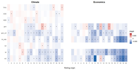
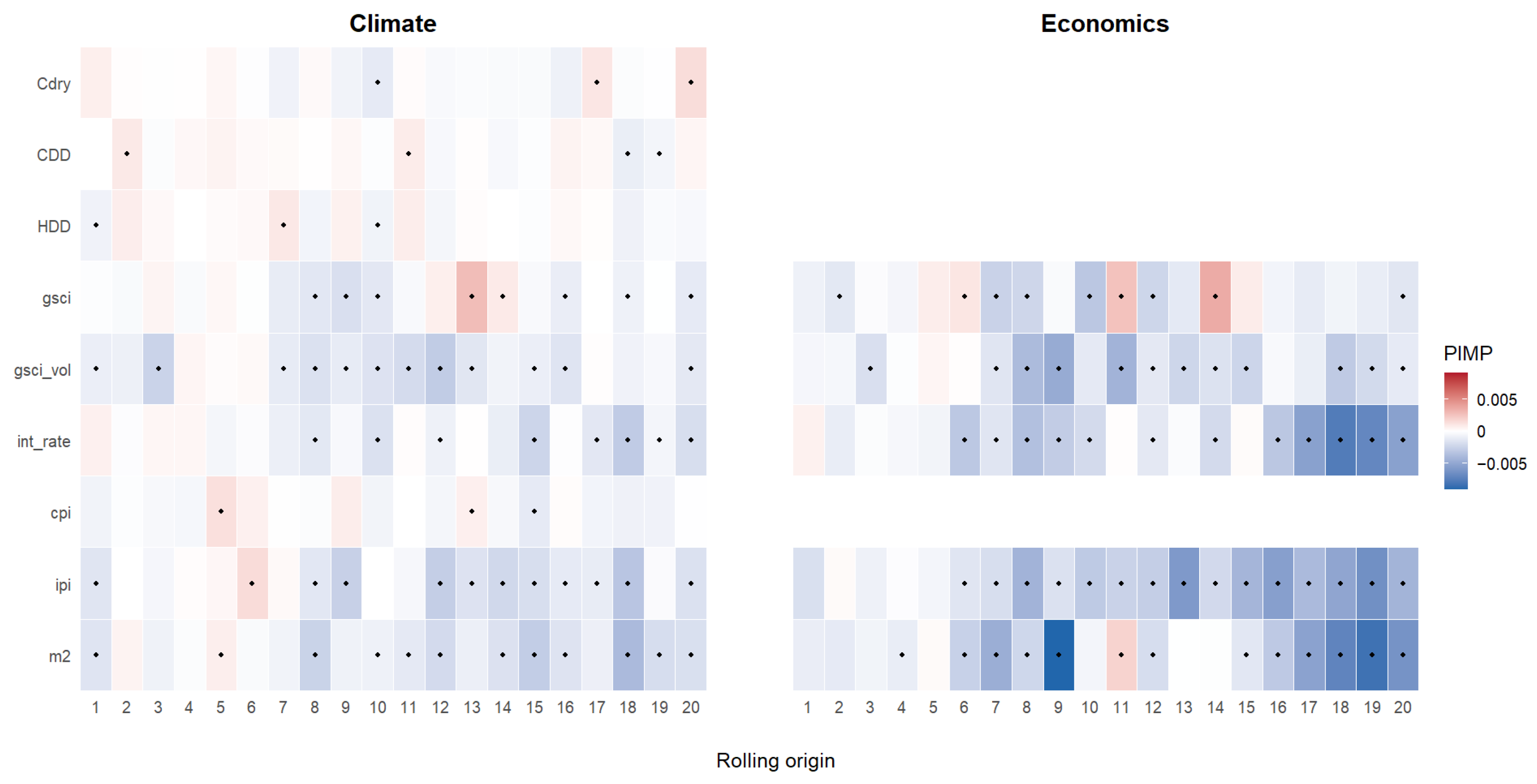
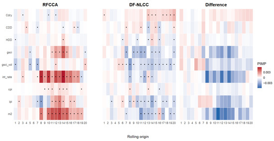
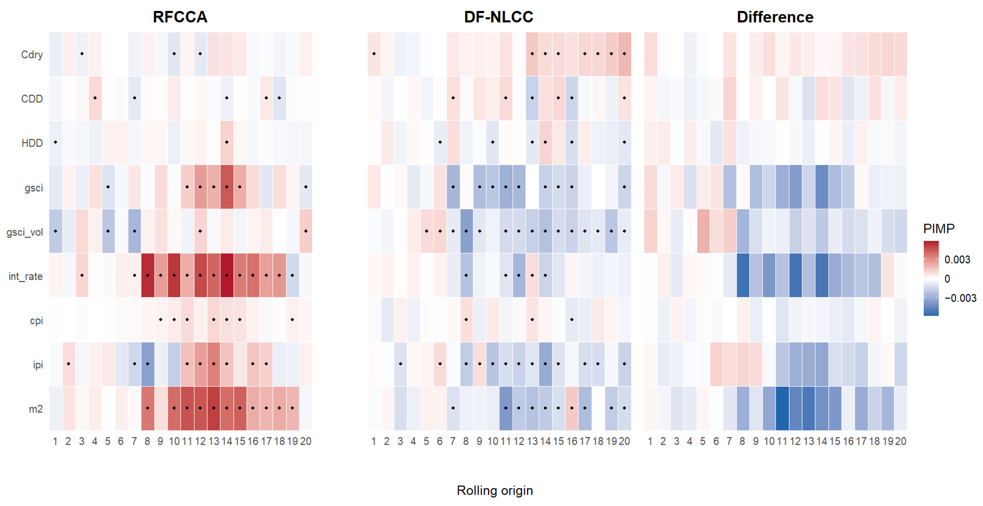
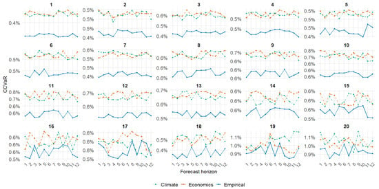
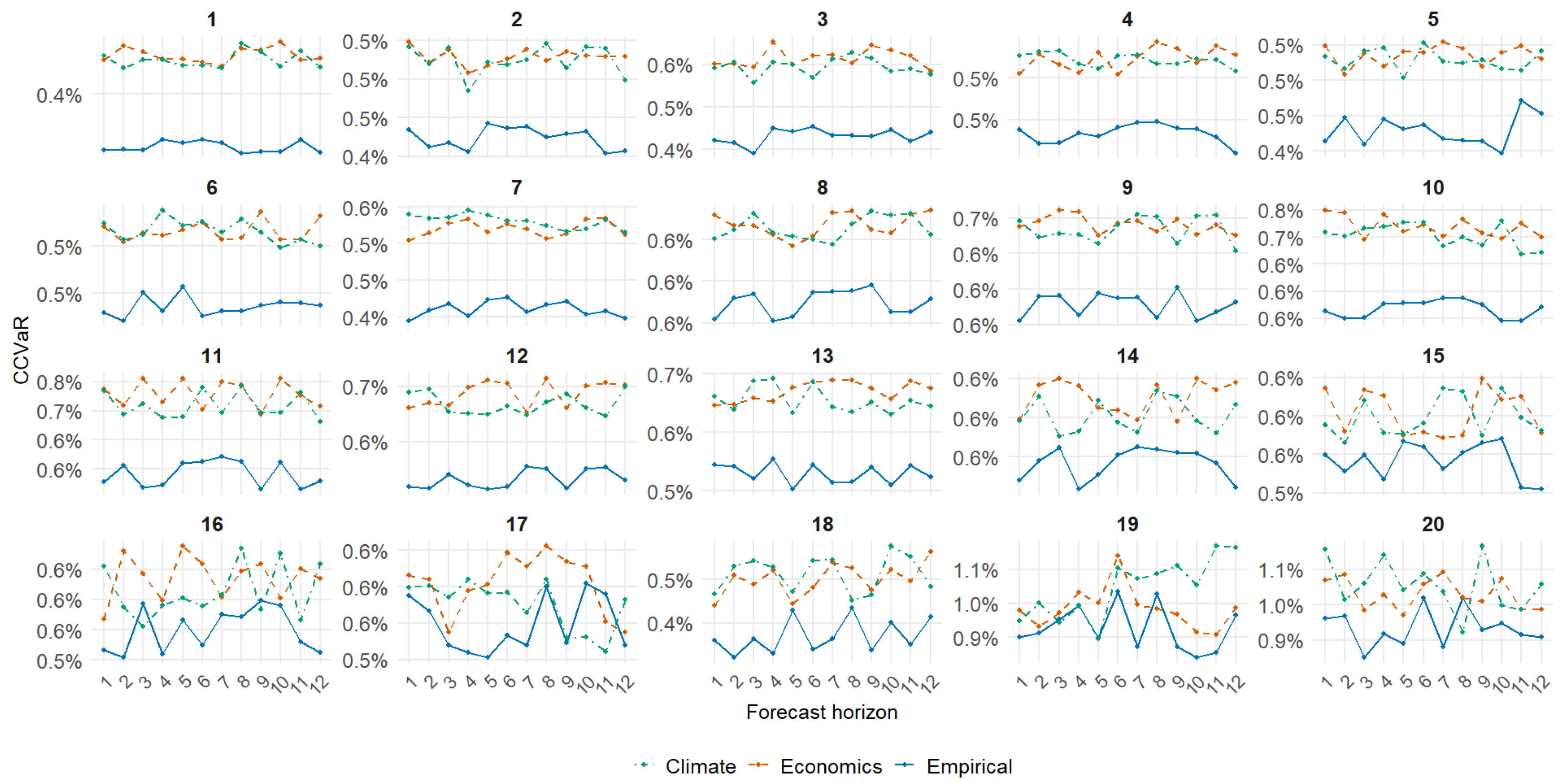
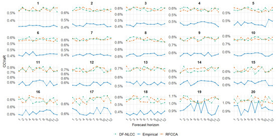
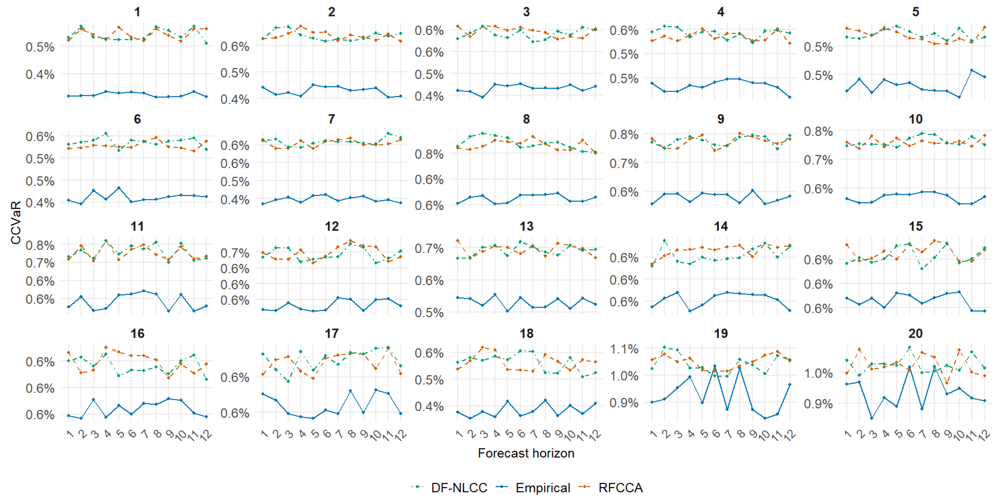

Disclaimer/Publisher’s Note: The statements, opinions and data contained in all publications are solely those of the individual author(s) and contributor(s) and not of MDPI and/or the editor(s). MDPI and/or the editor(s) disclaim responsibility for any injury to people or property resulting from any ideas, methods, instructions or products referred to in the content. |
© 2026 by the authors. Licensee MDPI, Basel, Switzerland. This article is an open access article distributed under the terms and conditions of the Creative Commons Attribution (CC BY) license.