


Abstract
Embedding an evolutionary algorithm (EA) into control structures offers an effective solution for specific control problems. Often, it predicts the best control values using a process model (PM). The primary limitation is its high computational time. Our work addresses optimal control problems (OCPs) with a final cost, using receding horizon control (RHC) with an EA as a predictor. This work is a continuation of a previous article, in which the EA predictor was replaced with a multilinear regression-based predictor. Our objective is to propose a predictor based on regression neural networks (RNNs) that emulates the behavior of the (EA, PM) couple. A number of closed-loop simulations using the existing EA controller produce sequences of optimal control values and corresponding state values, which are stored in a data structure. Datasets for each sampling period are derived from these data and are used to train RNN objects employing a unique RNN model. The model, which is an “optimizable” RNN plus the list of hyperparameters preset before optimization, is determined after a thorough analysis of possible candidates using a MATLAB R2025b application. The presented method of constructing an RNN predictor is the main contribution. Algorithms for (a) constructing the sequence of RNN objects and (b) simulating the closed loop are also proposed. A case study illustrates our method. The RNN predictor successfully emulated the (EA, PM) couple: (a) the control-loop dynamics were nearly identical; (b) the performance indices were essentially the same; and (c) the execution time of the controller significantly decreased from 38 to 0.054 s, demonstrating that RHC can be applied more broadly.
Keywords:
optimal control; evolutionary algorithms; machine learning; regression neural networks; simulation MSC:
68T05; 68T20; 68W50
1. Introduction
Many industrial processes, including biochemical ones, are repetitive and similar to batch processes. To control them, we first formulate optimal control problems (OCPs) and solve them using optimal controllers. A class of these controllers typically forecasts optimal control values within a prediction horizon using a process model (PM) as in [1], the continuation of which is presented in this article.
A control structure for implementing closed–loop optimal solutions is receding horizon control (RHC). The primary features of this structure include:
- a predictor that forecasts the best control values;
- a process model used to make the predictions.
The predictor employs a particular method to address the OCP, making metaheuristic algorithms, such as EA or particle swarm optimization, practical options [2,3,4]. Numerous articles emphasize how metaheuristic algorithms can tackle complex problems in dynamic optimization [5,6,7,8]. A systematic method for applying metaheuristics to solve OCPs is outlined in [9].
When implemented with an EA, the predictor has the following known traits:
- It can address complex optimization problems; this is the primary advantage, even when the knowledge is imprecise, incomplete, or uncertain, or when the problems involve nonlinearities or distributed-parameter systems [10].
- Its main disadvantage is its substantial computational complexity. During each sampling period, the predictor is called to generate a partial solution, which requires multiple numerical integrations.
- The execution time is significant and may occasionally be slightly less than the sampling period. Therefore, the EA predictor is usually employed to control slow processes.
- Several methods can decrease its execution time [11,12], but these methods tend to reduce the solutions’ accuracy.
Machine learning is a powerful tool used in a wide range of applications [13,14,15,16]. It provides an alternative solution to the primary potential weakness of the EA predictor.
When an exact solution does not exist, solving an OCP using RHC requires a metaheuristic to search for the optimal solution. The latter is equivalent to the optimal control profile (CP), namely the sequence of optimal control values. At each sampling period, the EA predictor solves a new optimization problem with the current process state as its initial state. It calculates the sequence of optimal control values over the remaining control horizon and sets its prediction to the first value in this sequence. Once the EA controller is achieved, we can write a simulation program for the closed-loop evolution over the control horizon that also records the optimal CP and state trajectory. By repeatedly executing this program M times (M being sufficiently large), we can generate data for an ML task (in particular, training data for RNNs).
The concept behind using an ML predictor is to employ a regression algorithm that mimics the behavior of the (EA, PM) couple. This means reproducing the EA’s mapping from the state vector (as the input) to the control value (as the output). In this way, we achieve an ML predictor that cannot construct the optimal solution but instead provides the optimal control value after training on data generated by the (EA, PM) couple. In real-time operation, the ML predictor would “read” (receive as input) the state vector from the actual controlled process.
In a previous study [1], the ML regression algorithm was represented by a set of multilinear regression functions, one for each sampling period. The authors investigated whether an ML algorithm could model the behavior of the (EA, PM) couple. They trained multilinear regression models [17,18,19] and designed an ML controller, which led to a significant reduction in execution time.
This work builds on the paper [1] by suggesting replacing regression functions with regression neural networks. Regression functions are limited in their ability to model the PM’s nonlinearities. RNNs are more elaborate regression models and can better capture (EA, PM) couples. However, this advantage will require more analysis work to find appropriate RNN models.
Our work is completely focused on a control structure called RHC [9,20,21,22], a kind of model predictive control [23,24]. RHC is devoted to implementing closed-loop control. The latter aligns with our desideratum of applying the proposed method to real-time implementations in which controllers must respond quickly and reject perturbations.
Given its importance, we shall present the new RHC structure in Section 2. In our case, its prediction module uses a version of the EA. For each sampling period, based on the PM, it predicts the new optimal CP up to the end of the control horizon. Then, the initial control value of the new CP is sent to the process, and the rest are neglected. At the next sampling time, the controller “reads” the state of the process and repeats its control cycle. In addition to the PM, other computations, including numerical integration, are used.
In this context, two predictors will be examined: (a) employing an EA and (b) using RNNs. Both structures manage the same process, address the same task, and employ the same PM. The controller obtained in case (b) will be referred to as the RNN controller. It will be implemented after the EA controller has been implemented. This last constraint ensures that a simulation program for the control-loop evolution can be written; it will be based on the EA controller.
More precisely, what does it mean to emulate the (EA, PM) couple? When a process state vector is presented to the EA predictor, the predictor sets its prediction, which will be the next optimal control value (the EA controller will send it to the process). That means the RNN predictor has to reproduce the EA’s mapping from the PM’s state vector to the control value as accurately as possible.
Simulations of the closed–loop evolution are performed using the EA controller, providing data to train the RNNs. The training data are split into datasets specific to each sampling period. The predictors are RNN objects (ready to predict), one for each sampling period. Each RNN is derived from a unique RNN model trained on the dataset corresponding to its sampling period.
In this work, the RNN model is an “optimizable RNN”, along with a list of hyperparameters preset before optimization; the remaining hyperparameters are established simultaneously during optimization.
The main objective of our work is to develop an RNN predictor that emulates the behavior of the (EA, PM) couple. In other words, the RNN controller would optimize the actual process in a manner similar to the EA controller. Section 2 will show more specifically the general objectives of our work and the practical targets.
To illustrate our presentation, we selected a well-known OCP, the Park–Ramirez problem (PRP), which is described in Appendix A. This is a benchmark problem exemplifying an OCP with final costs [25,26]. We emphasize the following points:
- This study does not directly focus on solving this issue;
- Addressing PRP allows for a comparison between the earlier approach with regression functions and the proposed approach employing RNNs;
- The PRP features a straightforward structure that keeps the presentation clear and uncomplicated.
Section 2 details the objectives of this paper and connects it to our previous work. To make the presentation self-contained, this section also presents a minimal set of theoretical elements concerning OCPs with final costs and their discrete-time solutions using an EA, while returning to the notation.
Section 3.1 goes over the materials used in this work. MATLAB and one of its applications were employed to develop the programs and to train and analyze the RNNs. In addition, some data, algorithms, and programs are taken from the previous work [1] and are considered materials for use in this research. Details on these materials are given in Appendix B, Appendix C and Appendix D.
The selection of the appropriate RNN architecture for the predictor that emulates the (EA, PM) couple is addressed in Section 3.2. The latter presents two stages of the research carried out: Stage I and Stage II; each involves a different approach and solution. The approach and solution proposed in this paper correspond to Stage II. The outcomes of Stage I are crucial because they lay the groundwork for Stage II’s approach. Stage I determines, for each sampling period, an RNN model; the latter is trained using its own training dataset. The result is an RNN object (ready to predict) devoted only to its sampling period. To conduct this stage, which involved analyzing a great number of models (over 200 for our case study), we used the Regression Learner application to select and train the RNN models. Moreover, Stage I’s solution is feasible only when the number of sampling periods is moderate. We need to analyze Stage I’s results to understand how to select the models in Stage II.
Stage II’s approach proposes using only one RNN model for all sampling periods. Only a few RNN models are analyzed before a single one is selected. This unique model is trained, for each sampling period, on the corresponding dataset, resulting in an RNN object. This solution is implemented by Algorithm 1 (in Section 3.2.2) and effectively builds the sequence of RNNs. Algorithm 2 (in Section 3.2.3) determines the closed-loop evolution using the proposed RNN controller, which includes the new predictor.
The two approaches are applied to our case study, and the results are presented in Section 4. Considering the number of models analyzed, the complexity of Stage I is incomparably greater than that of Stage II, even in our case study, where the number of sampling periods is moderate. For the Stage II approach, two RNN models are selected to serve as the unique model. In total, we present three situations, where the RNN controller is developed using the Stage I approach, Stage II—the first model, and Stage II—the second unique model. The RNN controller is built in the three cases, yielding very similar results. Algorithm 2 is used to obtain the optimal evolution of the closed loop over the control horizon. In all three cases, the CPs and the state trajectory are similar to those obtained with the EA controller.
The outcomes of this work, along with the related discussion, are presented in Section 5. The results produced by the Stage II approach convinced us that the main objectives were achieved:
- The control loop’s dynamics were essentially identical to those produced by the EA predictor, covering the optimal control profile and the state trajectory;
- The performance indices were essentially identical;
- The controller’s execution time diminished significantly, becoming even shorter than that of the controller achieved through regression functions. During a sampling period, thousands of PM’s numerical integrations are replaced with an RNN predictor call, resulting in significantly reduced execution times compared to the EA predictor.
The RNN predictor succeeded in emulating the (EA, PM) couple in a shorter execution time, demonstrating that RHC can be applied more broadly, even for fast processes.
The reader can reproduce the results presented in this paper using the scripts, functions, and workspaces included in the Supplementary Materials folder (see Appendix E).
2. General Objectives of This Work
To lay out the main goal of this work, we need to briefly present the scientific context of this research, which stems from the study of optimal control problems with a final cost. A realistic approach, developed by the authors, involves using receding horizon control with predictions generated by an evolutionary algorithm. Figure 1 presents the partial objectives related to this approach, numbered from #1 to #5. Behind each partial objective is an activity—called the same way—that leads to its achievement. The blue blocks represent the structures generated by these activities.
Figure 1.
Solving optimal control problems using the RHC strategy and EA prediction—using an RNN to emulate the (EA, PM) couple.
The authors have already addressed activities #1 and #2 in other papers [1,10,11,12,27]. In some cases, the simulation results show that the EA controller’s execution time is too long relative to the sampling period (even when the EA controller’s execution time is shorter than the sampling period). In these cases, an efficient approach is to implement the EA predictor using an ML algorithm that emulates the (EA, PM) couple. This is achieved through activities #3, #4, and #5 in Figure 1. To this end, the authors proposed a set of multiple linear regression functions in [1]. In this work, for the reasons already mentioned, the proposed ML algorithm is a regression neural network. Paper [1] also explains how to collect and use the dataset for training a machine learning model.
Remark 1.
The objectives of this work are to achieve the partial objectives #3–#5, namely:
- to find a suitable RNN that accurately emulates the (EA, PM) couple, that is, a new RNN predictor;
- to implement the new controller, called the RNN controller, using the RNN predictor;
- to implement a program that simulates the evolution of the control loop over the control horizon using the new RNN controller.
Instead, this work builds on the results of activities #1 and #2 reported in [1], as well as the generated structures (the EA controller and the datasets used to train the ML algorithm).
For example, in paper [1], Section 3.2, titled “Dataset generation for machine learning model”, describes how the training dataset is constructed. All results from that section are carried over and considered in this work. The ControlLoop_EA program, which performs closed-loop simulations and generates a quasi-optimal trajectory, is also used in this work.
Figure 2 more succinctly expresses the general objectives of this work. Briefly, the general objective is to go from (a) to (b) using a regression neural network when implementing the optimal controller. Although these variables are common in this context, their definitions are provided in the following subsections.
Figure 2.
The controller implementation using (a) an EA and (b) RNNs.
2.1. Optimal Control Problems with a Final Cost
We assume that the reader is familiar with an OCP’s structure. Therefore, below, we reference only the elements pertinent to the example in Appendix A (the PRP). To keep the presentation simple, rigorous mathematical details will be omitted.
The elements provided here recall the notation and ensure that the presentation remains self-contained.
2.1.1. Process Model
Since the RHC strategy is employed, the controller includes a PM made up of algebraic and ordinary differential equations. There are many types of PM, but we have chosen the one appropriate for our OCP.
—a vector containing n state variables;
—a vector containing m control variables;
W—a vector with parameters of the process.
The set of Equation (A1) in Appendix A is an example of a PM.
2.1.2. Constraints
We mention only the constraint types used in the Park–Ramirez problem, although there are many others.
The values represent the technological limits for .
The optimal control system’s sampling period is T. The control horizon is segmented into H sampling periods:
2.1.3. Cost Function
The OCP’s solution is the control function that optimizes (min or max) a specific cost function J, with the general form below:
The L function figures out the integral part (Lagrange term) of the J function, while (Mayer term) penalizes (or rewards) the final state.
Remark 2.
If the final cost appears in (5), regardless of the integral term, the endpoint of the prediction horizon must be the final time, which is the most computationally complex case.
Because of Remark 2, we consider that J reflects only the final cost, which aligns with our OCP (see PRP).
The OCP’s solution is the control function that yields the optimal value of the cost function. This value, denoted as J0, is also called the performance index:
2.2. A Discrete-Time Solution of an OCP Using an EA
The PRP was presented as originally formulated, that is, as a continuous-time problem. To align the elements of this OCP with the solution format obtained using an EA, the PRP was implicitly reformulated as a discrete-time problem. This reformulation involved some important aspects:
- the introduction of the state feedback (from );
- the time variable takes only the discrete values ;
- In the sequel, all operations performed within the RHC structure are discrete-time actions, including numerical integration. Any reference to time points within a sampling period is made to explain how the RHC structure and the real process are connected. For example, the control values, which are calculated only for k , are held at the input of the real process during the entire sampling period because it needs to be controlled at all times. This task is handled by a device (sample-and-hold) in the closed loop, interposed between the controller and the process being controlled. The task is characterized by the following equation:
Therefore, for the real process, the control variables are step functions. To keep things simple, the moment kT will now be called just k. For example, during the sampling period , it holds
A control sequence spanning the control horizon is called a “control profile” (CP). A CP will generate the diagram shown in Figure 3, where X(H) is the final state.
Figure 3.
A control profile generates a state trajectory with H + 1 states.
For each sampling period [k, k + 1), the EA produces candidate predictions covering the prediction horizon and their cost function values. A candidate prediction at step k is a sequence of control values, as follows:
If X(k) represents the process’s current state, it also serves as the starting point for candidate predictions. It is from here that the name “receding horizon control” stems. For each prediction candidate, the EA also generates its state sequence (with H − k + 1 states):
When the algorithm converges, it returns the optimal candidate prediction:
In our case, the candidate prediction that maximizes the cost function is chosen.Following the RHC strategy, the controller’s optimal output, denoted as U*, is taken to be V(k).
Its value will control the process. The leftover values in V(k) are neglected. Then, the controller will wait for the next sampling period [k + 1, k + 2) to compute its control value.
In the sequel, we refer to the optimal control value as U*(k) for simplicity, noting that it also depends on the current state.
Appendix B recalls a possible version of the predictor, Predictor_EA, structured as a function, that is used to calculate the optimal predictor at step k for the current process state X0. This predictor was also used to solve OCPs using the EA version developed in previous papers [19,21].
3. Materials and Methods
With the help of Figure 1, we specified the objectives of this paper. Because activities #1 and #2 are described in [1], we focus on activities #3, #4, and #5 to simplify the structure and presentation of this article.
3.1. Materials
This work builds on the results of activities #1 and #2 reported in [1]. Thus, we can use the algorithms and programs already developed. These programs accomplish two things:
- they implement the EA controller;
- they determine the dataset used to train the ML model.
Consequently, the algorithms and programs already available, along with the MATLAB system and its applications, are considered the materials used in this work.
In the following paragraphs, we provide a brief overview of these materials (a) to connect all the activities in this work logically and (b) to make the article easy to follow.
The list of materials carried over from the previous research [1] is given in Table 1.
Table 1.
List of materials used in this work.
To clarify which data are carried over from previous work, we recall some notation. The EA controller generates the best CP for the initial state X0 = X(0) by combining the optimal control values. Owing to this CP, the process passes through a series of “optimal states” that define the state trajectory :
These two sequences fully describe the optimal evolution of the closed loop over the control horizon. If the process and PM are identical, theoretically, the optimal cost function equals J0. In reality, the two values will be very close, so Ω(X0) is a quasi-optimal solution to our OCP.
Details concerning the use of the scripts, functions, and workspace files, which are materials carried over from [1], are provided in Appendix E. They can be skipped at the first analysis of this paper.
The MATLAB scripts, functions, and workspaces are included in the ART_Math folder, which is available to the reader as Supplementary Materials.
3.2. Methods
The structure of this section aligns with objectives #3–#5 in Figure 1 and their associated activities that guided our research. Before we tackle activity #3, let us recall how to generate the datasets for each sampling period, since we will need them when analyzing which RNN to choose.
3.2.1. Extraction of Datasets Characterizing Each Sampling Period
As in previous work, datasets are needed to train the ML model for each sampling period. Therefore, we recall the method used to generate these datasets, starting from the workspace (WS_data400.mat) that stores the optimal trajectories and CPs. For each sampling period k, a dataset is extracted from the STATE and UstarRHC data structures.
Given k, , we generate a matrix , which aggregates the states and optimal control sequences for step k across all M experiences.
Line i, , concatenates data from experience i:
Using the previously defined data structures, it holds that:
STATEi denotes the ith component of the cell array STATE. For our OCP, the content of SOCSK is explicitly given in Appendix D.
Algorithm A1 (Appendix D) presents the pseudocode for the data processing used to obtain the training and testing datasets for the RNN at each time step k. To save these datasets for each k, we will use the cell arrays DATAKTrain() and DATAKTest (). These will be used to train and test the RNN model later (Algorithm 1).
3.2.2. Determination of the Suitable RNN Structure
In this subsection, we analyze which RNN structure is suitable for the OCP at hand.
- N.B.:
- We aim to find an RNN that maps any PM’s state to the optimal control value. Moreover, the RNN does so in such a way that the control value is very close to what the EA predictor outputs under the same conditions. This requirement means that the RNN emulates the (EA, PM) couple.
- Stages of the research carried out:
- Stage I
We started our analysis with the hypothesis that each sampling period (denoted generically by k) has its own RNN that emulates the (EA, PM) couple. To determine this RNN, we used the Regression Learner application in MATLAB and conducted multiple construction sessions.
When selecting the suitable RNN for each k, we follow two interconnected objectives:
- (1)
- Determining the dataset size for each k = 0,…, H − 1. A subset that enables efficient training for the current RNN is selected from the data points in DATAKTrain{k};
- (2)
- Determining the best RNN for the selected dataset.
To avoid training inefficiency and overfitting to noise, we considered 2 or 3 subsets (denoted as ns(k)) of DATAKTrain{k} as datasets for the k-th sampling period. Let us denote them as Sk(i), i = 1, …, ns(k). For each k and i, we consider a number of RNN models (denoted as nmk(i)) to be trained on Sk(i).
We define a construction session as one in which the same training set Sk(i) and the same test set (DATAKTest{k}) are used to train all selected RNN models. Therefore, for each k, we have ns(k) construction sessions, in which we train a total of Ntrain(k) models.
For each k, we identify the best (most accurate) RNN across all its construction sessions. The best is the one with the lowest RMSE on the validation and test sets. Other statistical parameters, such as mean absolute error (MAE), mean absolute percentage error (MAPE), and R-squared, can also be used alongside RMSE to determine which is best. Objective (2) means recording the best RNN. We also record the set Sk(i0) used to train this RNN; this is objective (1).
This trained RNN is saved to implement the predictor for the k-th sampling period. Together with the best RNNs for all k values, it can implement the predictor over the control horizon, as we will see in the sequel.
- Stage II
At the end of Stage I, the examination of the RNNs across different values of k shows that a specific RNN model produced trained RNNs that ranked among the best. This is not an objective fact but rather a subjective one. Because of the high complexity of the construction sessions, we tested models that simultaneously cover many RNN parameters, that is, “optimizable” RNNs.
We observed and verified that the “optimizable” RNN was the best RNN model for each k, achieving the highest accuracy. We have also tested other architectures: Narrow, Medium, Wide, Bilayered, and Trilayered RNNs. The accuracy of the trained RNNs is better because the optimization process searches for the best combination of hyperparameters. At the beginning, we are tempted to let the Regression Learner application optimize all the hyperparameters at once, which leads to very long search times. Moreover, we are interested in having a unique model for all k. That is why we split the list of hyperparameters into two sub-lists: one containing those preset before training and the other containing those set during optimization. In this way, there are a few degrees of freedom for adjusting the unique model to each sampling period. For example,
| The list of preset parameters: | The list of hyperparameters set during optimization: |
| Number of layers | Activation function |
| Normalization of data | LayerSizes |
| Optimization type | Lambda |
Therefore, to have a unique model, we can consider, in addition to the RNN type, a list of preset hyperparameters. This implicitly determines the list of hyperparameters set during optimization.
There is a hard question: Does the unique model impose a hard constraint that might not be satisfiable, taking into account that each sampling period has its own training and testing datasets? There are two reasons for answering no to this question:
- -
- The system has state values at each sampling period that come from the same process. We can expect the datasets to keep a “trace” of this process;
- -
- The practical results justify this hypothesis of a unique model’s existence.
Therefore, in Stage II, we can use this RNN model along with the same list of preset hyperparameters. During training, the remaining hyperparameters are optimized for each k. Using a single RNN model for all k values greatly simplifies our preliminary analysis. In contrast, the datasets can differ and be adapted to the value of k.
Remark 3.
Stage II is a more realistic, feasible, and ultimately simpler approach proposed in this work. The RNN predictor will use a single RNN model with the same preset hyperparameters across all sampling periods. In contrast, the training and test sets will use the DATATrain{k} and DATATest{k} datasets, respectively.
Hereafter, we provide a sketch of how to select the unique model and generalize it for all sampling periods:
- We train a few models for 2–3 sampling periods (we already have the training sets). We identify 2–3 models (each will later serve as a unique model) to test and select the most suitable one. This research work is similar to Stage I but covers only 2–3 sampling periods.
- We select one of these candidate models, denoted as RNN0. This is also the model adopted for all sampling periods.
- Let k0 denote the sampling period that initially generates the model, which is considered a unique model, RNN0. Let i0 be the value such that the Sk0(i0) dataset yields the best-trained RNN derived from RNN0.
- For all , RNN0 is trained on the S(k) dataset. The latter meets the following constraints: (a) , and (b) S(k) has the same number of elements as the Sk0(i0) dataset.
- The H trained RNNs are used to implement the RNN controller and simulate the closed-loop behavior.
Repeating steps 2–5, we can select the most suitable RNN model. In addition, the implementation of the predictor and the controller is already achieved.
The constraint (b) from step 4 is optional; it is not mandatory. It was our choice to avoid a large number of data points (to avoid overfitting to noise), and it yielded good results.
- Construction sessions in Stage I
In Stage I, the research work is conducted by the designer of the RNN predictor (it is not automated); the designer is only assisted by the Regression Learner application (or a similar application) when choosing, training, and testing the RNN models. This is true for Stage II as well.
A construction session for k involves training multiple RNN models on datasets of varying sizes belonging to DATAKTrain{k}. Each RNN model is characterized by a set of hyperparameters and is subjected to the following:
- training, which yields an RNN object ready for prediction;
- testing using DATAKTest{k}.
In our case study, the total number of trained RNNs exceeded 200 in Stage I. After analyzing the results of the construction sessions for a specific k, the best RNN was identified, and its training function was saved. In total, H training functions for the best RNNs were saved.
The corresponding sizes of the training datasets were also stored in a vector named dimdata(1 × H). The training functions and the dimdata were stored in the DataStageI workspace for further utilization.
Algorithm 1 is designed to store the best results from Stage I. It creates, trains, and tests the “best” RNN for each k. We use this algorithm to compare the closed-loop behaviors with predictors developed by the Stage I and Stage II approaches. With very few modifications, Algorithm 1 can be used to implement Models-StageII (see Section 4.2).
| Algorithm 1: Models-StageI | |
| /* This pseudocode outlines the training and testing of the RNNs in Stage I, aiming to create the sequence of best models and the workspace file.*/ Input: workspace DataStageI./*It contains DATAKTest, DATAKTrain, and dimdata*/ Output: cell arrays: MODELNN{H × 1}, DATAKTest, and DATAKTrain (modified) store objects that are RNNs and tables, respectively, for each sampling period | |
| begin | |
| 1 | #load dimdata from DataStageI /* dimdata: vector (1 × H) with the datasets’ sizes determined in Stage I. */ |
| 2 | #load DATAKTrain{k} from DataStageI; |
| 3 | #load DATAKTest{k} from DataStageI |
| 4 | for k = 0…H − 1 |
| 5 | dataTest DATAKTest{k} |
| 6 | dataTrain lines 1—dimdata(k + 1) of DATAKTrain{k} |
| 7 | [mdlRNN, vrmse] trainRNN(k, dataTrain); |
| 8 | MODELNN{k + 1} mdlRNN |
| 9 | #compute the Root Mean Squared Error for the testing phase (RMSE). |
| 10 | #display vrmse (RMSE for the validation phase) and RMSE |
| 11 | end |
| 12 | #Save MODELNN, DATAKTest, DATAKTrain in the Models&Data workspace. |
| end | |
The DATAKTrain{k} table contains M–60 data points after download (340 in our case).
The best RNN models are stored in a cell array {H × 1}, MODELNN, similar to the training and testing data. The trainRNN function in instruction #7 takes k as an input argument and selects one of the H training functions determined in Stage I for the best RNNs.
RMSEtest and vrmse represent the root mean squared error for the test and validation phases. Finally, instruction #12 stores the models and data in a workspace file for future use.
Of course, we can obtain a general solution to our problem by providing an RNN model for each sampling period (k). Each model will be trained on datasets from the corresponding DATATrain{k}. In [27], the authors proposed only this approach, which yielded good results. The RNN predictor accurately emulated the (EA, PM) couple. For H = 15, this situation is acceptable even though more than 200 RNNs were analyzed during the construction session. This method becomes impractical when the number of sampling periods grows substantially, for example, to 100, due to the huge complexity of Stage I, which comprises too many construction sessions with the Regression Learner.
3.2.3. Simulation of the Closed Loop with RNN Predictor
If the RNN predictor is developed, we need a simulation program to study the closed-loop evolution and analyze its performance. This subsection introduces the ControlLoop_RNN algorithm, which employs RHC using an RNN predictor to emulate the (EA, PM) couple. The simulation over the control horizon is executed by a program unit, as detailed in Algorithm 2. Calling this function multiple times enables the generation of statistics.
| Algorithm 2: ControlLoop_RNN | |
| /* This pseudocode simulates the RHC functioning equipped with a controller that predicts using RNNs */ function [uRNN, FinalState, Jf]ControlLoop_RNN(MODELNN, X00) Input: cell array MODELNN{H × 1}; it contains a number of H trained RNN models; Outputs: uRNN—the sequence of the optimal control values; FinalState—the final state at the moment k = H; Jf—the value of the performance index. | |
| begin | |
| 1. | #Initializations: H, umin, umax, |
| 2. | #Allocate memory space for two arrays: uRNN(1, H) and state(H + 1, n);/*n = 5*/. |
| 3. | X0X00;/* X0 is the current state of the process during the simulation, X00 is the initial state at the start of the control horizon. */ |
| 4. | state(1, ~)X0;/*Store the initial state*/ |
| 5. | for k1 = 1…H;/* k = 0,…,H − 1; k1 = k + 1*/ |
| 6. | mdlRNNMODELNN{k1}; /* mdlRNN stores objects of type RNN, which are trained for the current sampling period*/ |
| 7. | uRNN(k1)The value predicted by the mdlRNN for the state X0. /* the optimal control value */ |
| 8. | #The value of uRNN(k1) is constrained within the established limits: umin and umax. |
| 9. | X0step_PP_RH(uRNN(k1),X0); |
| 10. | state(k1 + 1, ~)X0; |
| 11. | end |
| 12. | FinalStatestate(H + 1, ~); |
| 13. | Jfstate(H + 1,1) × state(H + 1,5); |
| 14. | #Display uRNN, FinalState, Jf |
| return | |
The vector uRNN(1, H) is gradually filled as the program runs, with the optimal control values being calculated and transmitted to the process. Finally, this vector represents a quasi-optimal CP. The “state” matrix records the process’s states, ultimately yielding a quasi-optimal trajectory.
Primarily, the simulation occurs through an interaction between the PM and the RNN Controller. The latter is implemented using instructions #6–#8; the mdlRNN model loads according to k1 and predicts the quasi-optimal control value for the current state, X0. Using the step_PP_RH function, instruction #9 calculates the process’s next state. The latter is computed via numerical integration using the current state and control input. The performance index, which characterizes the PRP, is calculated through instruction #13.
4. Results
4.1. Construction of RNNs for Each Sampling Period—Stage I
The results of Stage I are important to us because they form the basis for Stage II’s approach. A solution that uses a single RNN model is preferable to one that uses an RNN model for each k. However, we need to analyze the Stage I results; this analysis will allow us to consider and test the solution before concluding whether it is achievable.
The search for the best RNNs was conducted according to the method described in Section 3.2.2. The most important decisions were the selection of subsets Sk(i) because each one determines the dataset for a construction session. The choice of RNN models was made later, during each construction session.
Remark 4.
The selections of the subsets Sk(i) and the RNN models for different k values are not entirely independent. The experience gained in the first construction sessions helped the following selections because they refer to the same (EA, PM) couple. We repeated some choices that have proven to be effective.
Table 2 summarizes the quantitative aspects of our selections and presents some parameters characterizing the best RNNs.
Table 2.
The summary of the results of the research conducted in Stage I.
A few details need to be specified to clarify the activities performed to generate the best RNNs in Stage I:
- All selected RNN models were of the optimizable neural network type. The RNN models differ by the so-called “model hyperparameters”, that is, the list of parameters that are set before the optimal search for the other hyperparameters begins;
- The optimizer used in training all models is based on Bayesian optimization;
- The models can differ only by the so-called “hyperparameter search range” when only the ranges of variation differ;
- Each dataset involves carrying out a construction session;
- Each construction session involves (a) selecting a few RNN models and (b) training and testing these models;
- The best RNN is selected from all models trained across all construction sessions for the sampling period k. Its training function is generated and saved using the Regression Learner application.
Each line in Table 2 summarizes the results of dataset selection and training activities for each sampling period (k). To make the content of Table 2 easier to follow, we describe a few lines in correspondence with the sequence of actions that yield the data. For example, the following applies to line 1.
For the second sampling period, k = 1, we have selected five subsets S1(i), i = 1,…,5, from the training set DATATrain{1}. These subsets have the following sizes: 170(4), 190(9), 195(12), 200(4), and 250(3). The number of proposed RNN models for each dataset is shown in parentheses. The five construction sessions were completed, and all 32 models—column “Number of RNN models”—have been trained. The dataset with 190 data points yielded the best RNN model among all trained models, so it has been bolded.
A group of eight columns provides parameters for the best-trained and tested RNN. When the optimal training suggests two layers, the “Layer sizes” column shows two values separated by a comma. The “Stand. data” column indicates whether the training data are standardized (normalized). The RMSE parameter, a key metric for selecting the best model, is reported for both phases: validation (during training) and test (on unseen data points).
The case k = 0 is special because the initial state, which is known and reproduced in practice for technological reasons, has x1 = 0 and x2 = 0. Therefore, only three predictors require a smaller dataset than the other k values.
After the first two values of k, the number of datasets selected for the remaining k values was reduced to two or three. Understanding the learning process confirms Remark 4.
If we want to develop an RNN controller using the “best” RNNs identified in Stage I, as we did in [27], we must use Algorithm 1 to organize the RNN objects (ready to predict) into a workspace. In turn, Algorithm 1 needs some input data:
- the dimdata vector containing the dataset sizes;
- the training functions for all the best RNNs.
Table 3 taken from article [27], shows the elements of the dimdata vector saved in the dataStageI workspace.
Table 3.
The size of the training data for the best RNN at each k (taken from [27]).
After several construction sessions, we identified the key features of the models we can use. Table 4, taken from article [27], summarizes these characteristics.
Table 4.
Characteristics of the construction sessions (taken from [27]).
For example, for k = 10, the RNN that achieves the best accuracy is the “optimizable” neural network trained on 190 data points and tested on 60 unseen data points. The chosen optimizer was Bayesian optimization. The resulting optimizable hyperparameters and the training results are given in Table 5, taken from article [27].
Table 5.
The optimized hyperparameters and the training results for k = 10, taken from [27].
4.2. Determining a Single RNN for All Sampling Periods—Stage II
For a large H, training many RNNs during construction sessions is tiring and possibly infeasible. In fact, the whole point of this work is to skip Stage I and provide a simpler, more practical solution.
Remark 5.
The method presented in Stage I can be used for a control loop with a moderate H value.
After the analysis produced in Stage I, we have noticed that a single RNN model can be used for all k values. This single RNN model must be trained and tested on datasets that can differ and be adapted to the value of k. Finally, we always obtain H regression neural networks that are ready to predict, one for each sampling period, and these are determined and stored automatically.
The procedure for the determination of RNNs has the following steps:
- Select only a few k values for which we develop construction sessions. For example, k = 8 and k = 10 were selected. An RNN0 model, along with its training function F0 and dataset size n0, is selected from the best models generated during the construction sessions.
- For each k, an RNN object is trained using the F0 function, DATAKTrain{k}, and DATAKTest{k}. This is performed by the Models-StageII algorithm, which is not provided in this article because it is practically identical to Models-StageI except for instruction #7. The training does not depend on k because the training function F0 is used for all k. This time, all elements of the dimdata vector equal n0. All resulting RNNs are saved in a workspace for future use.
- The ControlLoop_RNN program implements the RNN controller and simulates the closed-loop evolution. The optimal CP and trajectory are shown, along with the final state and the performance index.
Because we conducted many construction sessions in Stage I, this time we took, for example, the best RNN constructed for k = 10. The regression model will be denoted by RNN10, and its training function by F10. To demonstrate that the method is robust to the choice of RNN model, we also implemented a case in which the controller uses RNN8. The optimized hyperparameters and the training results for k = 8 are given in Table 2.
To compare the impact of different controller implementations on the control loop’s evolution, we present the CP and the state trajectory for each variant.
Figure 4 presents the two curves that characterize the quasi-optimal regime of the control loop: the CP and the state trajectory, when the controller is implemented with the EA predictor in its initial variant. We present Figure 4 as a reference for comparison with the other graphical results developed in this work. The solution presented here is the optimum found in our previous work, which uses an EA directly. The optimal CP and state trajectory had already been saved in a workspace file.
Figure 4.
Quasi-optimal evolution of the closed loop when the controller uses the EA predictor.
The research conducted in Stage I and Stage II involves two implementation methods for the RNN controller. The closed-loop evolution is presented below for both methods.
Figure 5 presents this evolution when the RNN controller uses a distinct RNN for each sampling period, that is, for each k. The best RNNs are described in Table 2.
Figure 5.
Quasi-optimal evolution of the closed loop when the controller uses an RNN model for each k (Stage I).
Figure 6 highlights a key finding of this paper. It presents the evolution of the control loop when a single RNN model is used. Datasets for each sampling period are used to train the single model, yielding RNNs that are ready to predict. The truth value of this result is determined by comparing it with Figure 5.
Figure 6.
Optimal evolution of the closed loop when the controller is generated using RNN10 as a single model.
The RNN model that generates Figure 6 is RNN10, as described earlier. Figure 7 presents the two curves when RNN8 is the sole model.
Figure 7.
Optimal evolution of the closed loop when the controller is generated using RNN8 as a single model.
Because the performance index Jf is essential for an OCP, Table 6 presents its values for all implemented variants.
Table 6.
Performance index for each implementation.
Along with the performance index, the execution time of the controller implementing the RHC structure is an important result, being an initial objective of our research. Table 7 provides the execution times of the controllers proposed in this work.
Table 7.
Execution time for the developed controllers.
For the RNN controllers proposed in this work, execution time is a random variable due to the stochastic nature of RNNs that emulate an EA metaheuristic. The statistics shown in Table 7 are based on 50 runs of the ControlLoop_RNN program.
5. Discussion
All the general objectives stated in Remark 1 are addressed by the methods and results presented earlier.
5.1. Differences Between the Approaches Generated by Stages I and II
Partial objective #3 is primarily addressed in Section 3.2.2. The Nota Bene clearly explains what it means to emulate the (EA, PM) couple. The predictor of the RHC structure depends not only on the EA (its version) but also on the PM that interacts with the EA.
There are two approaches presented in Section 3.2.2, each described as a stage of the same research work: Stage I and Stage II. The novelty of this paper lies in the approach presented in Stage II, which enables simpler implementation of an RNN controller, even when H is quite large. Both stages were presented to better explain Stage II by comparison. The simplification of the construction sessions introduced in Stage II can be observed only after analyzing Stage I’s results. In [27], an initial version of the Stage I approach is described, and the RNN controller is implemented. We took the results and present them here in a more detailed, implementation-oriented manner.
In Stage I, determining the “best” RNN for step k is a complex task that involves several construction sessions. Moreover, the two objectives, determining the best RNN model and its dataset size, depend on each other.
Remark 6.
Given the complexity of this task, the preferred RNN type for each model was the “optimizable RNN”. The RNN model is the RNN type plus the list of hyperparameters set before optimization; the remaining hyperparameters are learned simultaneously during optimization.
The designer conducting Stage I uses the Regression Learner application and manually creates the DataStageI workspace. Algorithm 1 automatically takes over the data from DataStageI, creates the best RNNs, and saves them in the Models&Data workspace for future use (for implementing RNN controllers and control-loop simulation).
We can better understand Stage II by highlighting its differences from Stage I:
- Stage II is a shortened version of Stage I. Stage I yields H “best” RNN models, one for each sampling period. Stage II proposes a single “best” RNN model for a specific k, which is then extrapolated to all the sampling periods.
- Stage II is a necessity when H has high values. In these cases, Stage I may be infeasible due to the very large number of construction sessions that are performed manually.
- When H is moderate, the Stage I results can be used directly to implement the RNN controller; in this case, the Stage II results can also be used to implement the RNN controller, with a single RNN model for all sampling periods.
- The controller implemented using the Stage I approach uses RNNs that, by construction, are adapted to their sampling period. In contrast, in the Stage II approach, the controller uses a single model that is adjusted for each sampling period by training and testing it on its own dataset.
Because a single RNN model is extrapolated to all sampling periods, one can ask whether this approach is effective. The response is positive for two reasons:
- ➢
- The single RNN model is “adjusted” for each sampling period by training and testing it on its own dataset.
- ➢
The second argument must be verified when solving other OCPs; in these cases, prediction accuracy must also be carefully analyzed.
The main quality of Stage II’s approach is that it is always feasible, as it involves only a small number of construction sessions with the Regression Learner application (or a similar one).
5.2. Implementation of the RNN Controller and Simulation of the Closed-Loop Evolution
Partial objectives #4 and #5 from Figure 1, namely the controller implementation and the simulation of the closed-loop evolution, are addressed simultaneously by Algorithm 2 (the ControlLoop_RNN function) in Section 3.2.3. Some details must be emphasized.
This function uses the collection of RNN objects, one for each sampling period, regardless of the approach (Stage I or II). This collection is named MODELNN and is composed of RNNs trained, tested, and ready for prediction, stored in a cell array.
Before calling the Algorithm 2 function, the Models-StageI script or the Models-StageII script (not provided in this paper) generates the MODELNN collection. The Models-StageII script has only two particularities that are worth emphasizing:
- -
- The training function F0 is used for all k;
- -
- All elements of the input dimdata vector equal n0. In this way, all the datasets have the same size but belong to different sets of DATAKTrain{k}.
5.3. Comparison of Optimal Control Profiles, State Trajectories, Performance Indices, and Execution Times
The novelty proposed in this paper is an approach (Stage II) in which the following occur:
- an RNN model addresses the objective shown in Figure 2;
- the RNN controller is effectively implemented and simulated.
We have executed the ControlLoop_RNN simulation program multiple times to observe the new RNN controller in action. The control profile and state trajectory shapes, as well as the final performance index, were the main interest for us.
A comparison was made between four evolutions of the closed-loop system, using four controllers:
- the EA controller: RHC with predictions made by the EA (Figure 4);
- an RNN controller conceived within the Stage I framework: each trained RNN is associated with a specific sampling period of the control horizon and predicts the optimal control values for that period (Figure 5);
- an RNN controller using the Stage II approach: a single RNN model (RNN10) is associated with all sampling periods, but it is trained on the dataset specific to each sampling period (Figure 6);
- an RNN controller using the Stage II approach but using RNN8 as the single RNN model (Figure 7).
Analyzing the four figures, the following conclusions can be drawn:
- ▪
- The quasi-optimal CPs are very similar, which explains why the two performance indices are almost equal (Table 6);
- ▪
- The three RNN controllers successfully emulated the optimal behavior of the (EA, PM) couple, which was our goal.
Due to its importance, we evaluated the controllers’ execution times during the closed-loop evolution over the control horizon. We executed the ControlLoop_RNN simulation program 50 times under the same initial conditions because of its stochastic nature. Table 7 shows an outstanding decrease in execution time relative to the EAcontroller’s time. This extends the use of RHC to include not just slow processes but also fast ones with small time constants.
5.4. Aspects of Designing the RNN Controller
To better understand the novelty of the RNN controller proposed in this work (the Stage II approach), we highlight a few aspects in the sequel. In this subsection, we consider the design procedure for developing an RNN controller for real-time use.
The design procedure for the RNN controller can be described in the following steps:
Design procedure
- (1)
- The script LOOP_M runs the already existing function for closed-loop simulation using EA (ControlLoop_EA, Appendix C) M times. It generates M optimal trajectories and CPs and stores them in a workspace.
- (2)
- Extraction of datasets characterizing each sampling period (Section 3.2.1).
- (3)
- Determination of the suitable RNN structure using the Stage II approach (Section 3.2.2).
- (4)
- Run Models-StageII (Algorithm 1, lightly modified, Section 3.2.2) and produce a collection of RNN-trained objects ready for prediction, one for each sampling period.
- (5)
- Carry out ControlLoop_RNN (Algorithm 2, Section 3.2.3) to implement the controller and simulate the closed-loop evolution.
The RNN controller design procedure is carried out offline. Let us note the following aspects:
- ▪
- Within the RHC framework, the EA predictor relies solely on the PM and does not consider other information from the actual process.
- ▪
- A key part of the design procedure is gathering training data offline by repeatedly simulating the closed loop over the control horizon. We want to clarify that gathering training data offline through simulations is not required simply because the work described here is a simulated study, but because we need to characterize the (EA, PM) couple.
Remark 7.
Although the RNN controller sends control values to the actual process, the training data are gathered via simulations. This is accomplished using a program such as ControlLoop_EA.
In other words, the RNNs must “learn” the dynamics of the (EA, PM) couple. Data from the real process are not needed in this phase. Usually, these data are considered during PM development.
The construction sessions, RNN model training (for each sampling period), and closed-loop simulations are also conducted offline.
5.5. Predictions Map the Actual Process States
We keep the perspective of an RNN controller designed for real-time applications. Its control action involves predicting the control output based on the actual process state.
Remark 8.
The state vectors sent to the RNNs for prediction differ from those used during training. Specifically, the PM does not perfectly model the actual process. They differ somewhat. Therefore, the “read” states from the actual process differ from those in the training data.
To what extent does the difference between the PM and the actual process influence the solution’s quasi-optimality? We have proposed a possible response to this question in [27] (Section 4.3.3). We characterized the actual process symbolically at the level of the state variables with the following expression:
actual process = PM + an additive perturbation.
Using a practical approach (a simulated study of the PRP), we showed how to estimate the extent to which the control loop deviates from quasi-optimal behavior.
5.6. Broader Applicability of the Proposed Method—Distributed Parameter Systems
RNNs are complex regression models and can better capture nonlinearities and other types of dynamics. For this reason, we have chosen RNNs to replace multilinear regression functions. The PRP features a dynamic model characterized by significant nonlinearities, and the use of RNNs yields strong, convincing results. This case study is sufficient to understand the methodology we proposed, which shows how to systematically obtain an RNN predictor. However, to better demonstrate RNNs’ ability to capture complex dynamics, we show below how the Stage II approach can solve an OCP involving a distributed-parameter system. Our goal is to show that the proposed method for obtaining the RNN predictor and controller is also applicable to these processes.
Paper [10] addresses controlling microalgae growth in a specific, artificially lit photobioreactor (PBR) that was physically constructed. A continuously stirred flat-plate PBR, illuminated on one side and operating in batch mode, is described. We are interested in producing biomass (microalgae) using light energy. Controllers can adjust the incident light intensity to control variables such as the light-to-microalgae ratio and biomass yield per unit of light energy. The PBR has a depth, L, through which light passes among microalgae. Therefore, the microalgae are irradiated according to their depth z (z ∈ [0, L]). The irradiance is related to the biomass concentration (x), the depth of the culture (z), and a few coefficients: the mass absorption (), the mass scattering (), and the backward scattering fraction (b).
q0 is the incident light intensity. Because the irradiance, specific growth rate, and other parameters depend not only on time but also on the physical position (z), we are dealing with a distributed-parameter process.
To formulate a control problem, we replace q0 with the control input q(t), which varies according to the control objectives. We stated an OCP involving this PBR in the general context of this work. In this case, the PM corresponds to a distributed-parameter process. A common method for dealing with this kind of process is to convert it, through discretization, into a lumped-parameter process.
The three components that define this OCP are listed below.
- 1.
- Process model (PM):
We converted the PBR’s process into a lumped-parameter model. Its depth, L = 0.04 m, is discretized into kL () equally spaced points . Once discretization is complete, the PM is represented as follows:
where
The PM constants are given in Table 8. The control input u(t) represents the intensity of the incident light.
u(t) = q(t).
Table 8.
The PM constants (taken from the authors’ article [10]).
The state variables are listed below:
: the biomass concentration (in g/L);
: the amount of light that has illuminated the PBR up to moment t (in µmol/m2/s). This state variable will be included in the process model solely when PBR productivity needs to be assessed.
The biomass m(t), calculated using Equation (15), serves as the product of the PBR.
- 2.
- Constraints
The PM has to meet the following constraints:
control horizon: t0 ≤ t ≤ tf;
initial conditions: x(t0) = x0
bound constraints: qm ≤ q(t) ≤ qM, with t0 ≤ t ≤ tf.
t0 and tf are the initial and final times of the control horizon; qm and qM are the minimum and maximum values of the admissible light intensity.
Productivity constraint:
where is the newly produced biomass at the final time.
- 3.
- Cost function
The cost function (21) represents the amount of light used for the current batch, subject to constraint (20). The two weight factors ( and ) are established through simulation.
Reducing the first term results in less light, whereas a small terminal penalty indicates that the goal m0 has been reached. Therefore, the PBR must produce m0 biomass with a minimum amount of light. The solutions for which are rejected by the EA, so when J is calculated. It is obvious that for the optimal solution, because the PBR would use less light, which aligns with the optimization objectives. In practice, we shall obtain a very good quasi-optimal solution.
To implement the RNN predictor and controller, we applied the design procedure presented in the previous section.
Applying the Stage II methodology, we selected the RNN as the sole model for all 120 sampling periods. Drawing on our experience solving this OCP, including work with other metaheuristics on the same OCP, we have set the following parameters:
Number of Layers: 3
Activation functions: relu| tanh| sigmoid| none—determined through optimization;
Lambda: determined through optimization;
IterationLimit for optimization: 500;
Standardize: true;
The remaining parameters are determined for each sampling period using specific training data. Finally, we have 120 trained and tested RNNs.
By running the ControlLoop_RNN program, we simulated the evolution over the control horizon using the RNN controller. We recall that the latter uses all 120 RNNs, one for each sampling period. The evolution is shown in Figure 8a,b, using data from a previous study on the same OCP.
Figure 8.
(a) Optimal CP for the photobioreactor OCP; (b) state evolution and the produced biomass.
The curve for x2 is not a perfectly straight line. It is close to a straight line because it is the result of the integral term, with q(t) having moderate variations. The program displays some useful information at the end:
Elapsed time is 1.091915 s.
final state:
x1 = 2.4459 x2 = 9.3116
&&& x00 = 0.3600 yield mass = 3.0245 Light = 9.3116 J = 9.5567
The time displayed corresponds only to the control action. The target m0 (we have a bilocal optimization problem) is reached with 0.81% precision. The amount of light used for the current batch is 9.3116 µmol, and the performance index is J = 9.5567 (w1 = 1, w2 = 10). Using the definitions, we calculated the penalty term of J:
Verification: = 9.3116 + 0.245 = 9.5566
The 120 RNNs, which serve as predictors for all sampling periods, were trained and tested using data collected from a simulation of 200 evolutions over the control horizon. The dataset for the accuracy test contains 60 values for each sampling period. The RMSE values for both the validation test (during training) and the test phase (using values not used in training) were recorded. Figure 9 displays these values for each RNN, corresponding to each sampling period.
Figure 9.
RMSE for the RNNs corresponding to all sampling periods.
The RMSE refers to the light intensity, which is the control input of the PBR. It ranges over the interval [85, 170], which is not excessive given the large range of light intensity, [50, 2000] . By comparing the average values of both RMSE sequences, the situation becomes clearer:
Average(RMSE training) = 125.5; Average(RMSE test) = 124;
The test confirms the validity of RNN training and the generalization capability of the RNN predictors.
5.7. Are the RNN Controllers Generally Replacing the EA Controllers?
This question is asked in the context of RHC and has the following meaning: Could the EA metaheuristic be replaced with a proper RNN from the outset of the controller design process?
For a quick answer, let us imagine that we should make a small modification to the PM. In this case, we need to restart the design procedure, including M simulations of the closed loop to create new training data. This occurs despite the EA remaining unchanged. Therefore, it could not.
Let us note two aspects that are part of a more elaborate answer:
- To solve an OCP using RHC, the controller needs a metaheuristic that searches for the optimal solution, that is, the optimal CP. At each step, the EA predictor first solves the OCP and then predicts the optimal control value as being the first value of CP. The RNN predictor only mimics the behavior of the (EA, PM) couple, that is, the mapping between the state vector (as input) and the control output. The RNN predictor cannot find the optimal solution; it only emulates the behavior of the (EA, PM) couple and predicts the optimal control value, leveraging its generalization power.
- Our goal was stated from the beginning: that we look for RNNs that emulate the (EA, PM) couple, which is possible.
Remark 9.
If the RHC solves an OCP using an EA, it would begin with constructing the EA predictor. The RNN predictor will be developed only after designing and simulating the EA controller to generate training data. In this context, the RNN controller serves as a faster version of the EA controller.
Therefore, the EA remains a metaheuristic that is worth considering in the context of RHC for difficult OCPs.
6. Conclusions
Within the RHC context, this work demonstrated that a set of regression neural networks can emulate the optimal behavior of the (EA, PM) couple. As a result, the RNNs can now implement the predictor of the optimal controller. Each sampling period has its own RNN object ready to predict. The RNN is the result of training a unique RNN model—one model for all sampling periods—using the dataset specific to each sampling period.
RNNs can model more complex systems than the multilinear regression functions addressed in the previous paper [1]. The price of this greater capacity to model complex processes is the analysis required to find the single RNN model used for all sampling periods. This unique model is an “optimizable” RNN along with a list of hyperparameters preset before the optimization process begins. The Regression Learner application in MATLAB, or a similar application, can help identify this model. We have also solved other OCPs with essential nonlinearities using RNNs, achieving good results, as in this work.
The solution presented in this work (the Stage II approach) is an improvement over another (the Stage I approach), in which each sampling period has a distinct RNN model. Regardless of the number of sampling periods, only the newly proposed solution is always applicable because the analysis required to identify the unique RNN model is much less complex.
The simulated RNN control loop outperformed the EA control loop, demonstrating very good performance:
- Comparable optimal control profile and state trajectory;
- A quasi-equal performance index, indicating that the solution’s optimality is maintained;
- The execution time of the RNN controller is even shorter than that of the regression-based controller; it decreased remarkably from 38 to 0.054 s.
In addition to the quantitative features mentioned earlier, there are other characteristics of the proposed approach to constructing the RNN controller that are worth noting:
- The training data are generated by simulating the control loop using the EA controller, along with an actual process identical to the PM;
- No actual process data are necessary since only the (EA, PM) couple determines the optimal control value for each sampling period;
- In real time, the RNNs make predictions using the state vector, which is “read” (received) from the actual process, not from the PM.
The RNN predictor and controller are simply more efficient versions of the EA predictor and controller, respectively, so EAs will remain relevant for certain optimal control tasks.
Supplementary Materials
The following supporting information can be downloaded at: https://www.mdpi.com/article/10.3390/math14173239/s1, The archive “ART_Math.zip” contains the files mentioned in Appendix A, Appendix B, Appendix C, Appendix D and Appendix E.
Author Contributions
Conceptualization, V.M.; methodology, I.A. and V.M.; software, V.M.; validation, V.M. and I.A.; formal analysis, V.M.; investigation, I.A.; resources, I.A.; data curation, I.A.; writing—original draft preparation, V.M.; writing—review and editing, V.M. and I.A.; visualization, I.A.; supervision, I.A.; project administration, I.A.; funding acquisition, I.A. All authors have read and agreed to the published version of the manuscript.
Funding
This research received no external funding.
Data Availability Statement
The original contributions presented in this study are included in the article. Further inquiries can be directed to the corresponding author.
Acknowledgments
This work benefited from the administrative support of the Doctoral School of “Dunarea de Jos” University of Galati, Romania.
Conflicts of Interest
The authors declare no conflicts of interest.
Abbreviations
The following abbreviations are used in this manuscript:
| RHC | Receding Horizon Control |
| OCP | Optimal Control Problem |
| PM | Process Model |
| EA | Evolutionary Algorithm |
| CP | Control Profile |
| RNN | Regression Neural Network |
| ML | Machine Learning |
| PRP | Park–Ramirez Problem |
Appendix A
An OCP with a Final Cost
The Park–Ramirez problem is a benchmark illustrating a final-cost optimal control problem. The nonlinear model illustrates a fed-batch reactor that is used to produce secreted proteins. It has been widely studied, particularly regarding integration methods:
The meanings of the state variables are as follows: —concentration of secreted protein, —concentration of total protein, —density of culture cells, —concentration of substrate, and —holdup volume.
It holds n = 5; m = 1; .
Constraints:
Performance index:
An open-loop solution cannot be implemented in real time due to the differing dynamics between the actual process and the process model, even if the differences are minor; this can result in inconsistent performance or instability. Our aim is to create a controlled, optimal process (a closed-loop solution) starting from a specified X0, using the previously defined performance index.
Appendix B
Predictor for Step k and Initial State X0 Using a Version of an EA
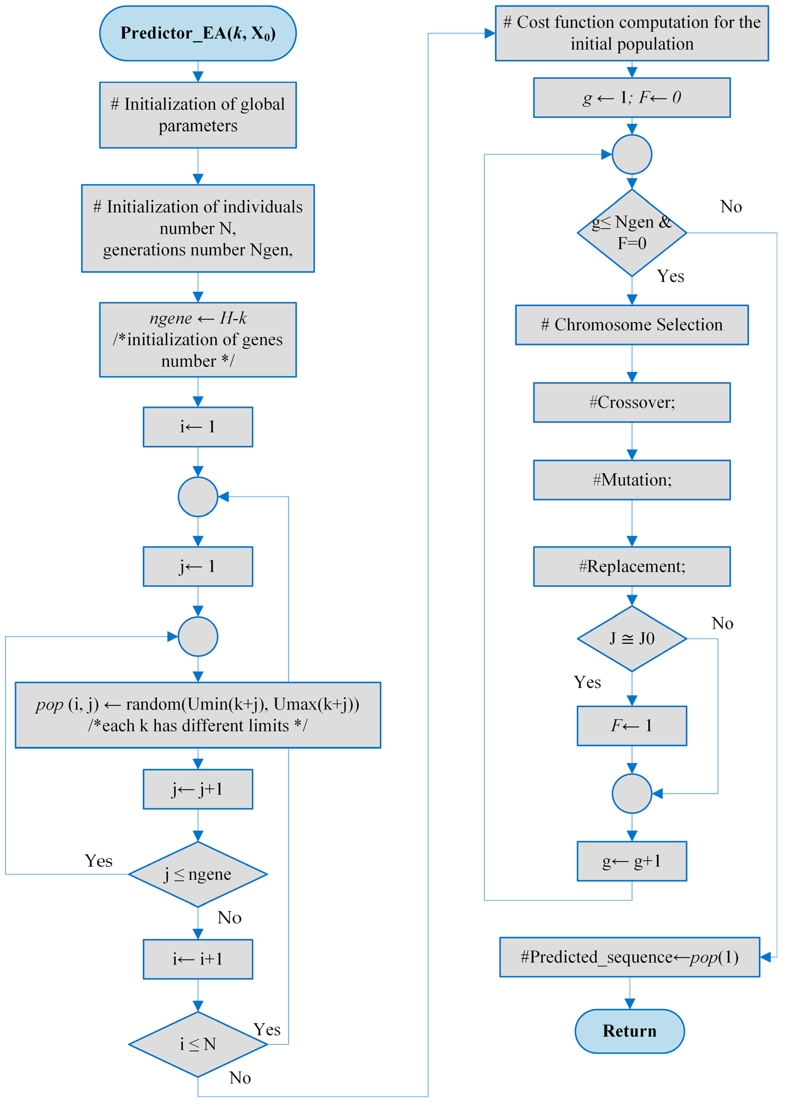
The offspring’s cost values are determined by the EA’s operators. Variable F is used to terminate the iterative process when the algorithm converges. When the performance index approaches J0, the EA terminates, indicating that a highly satisfactory solution has been identified. The predicted control sequence is the best solution identified by the EA.
Figure A1.
The flowchart for the EA predictor.
Appendix C
Simulation of Closed-Loop Evolution over the Control Horizon Using RHC
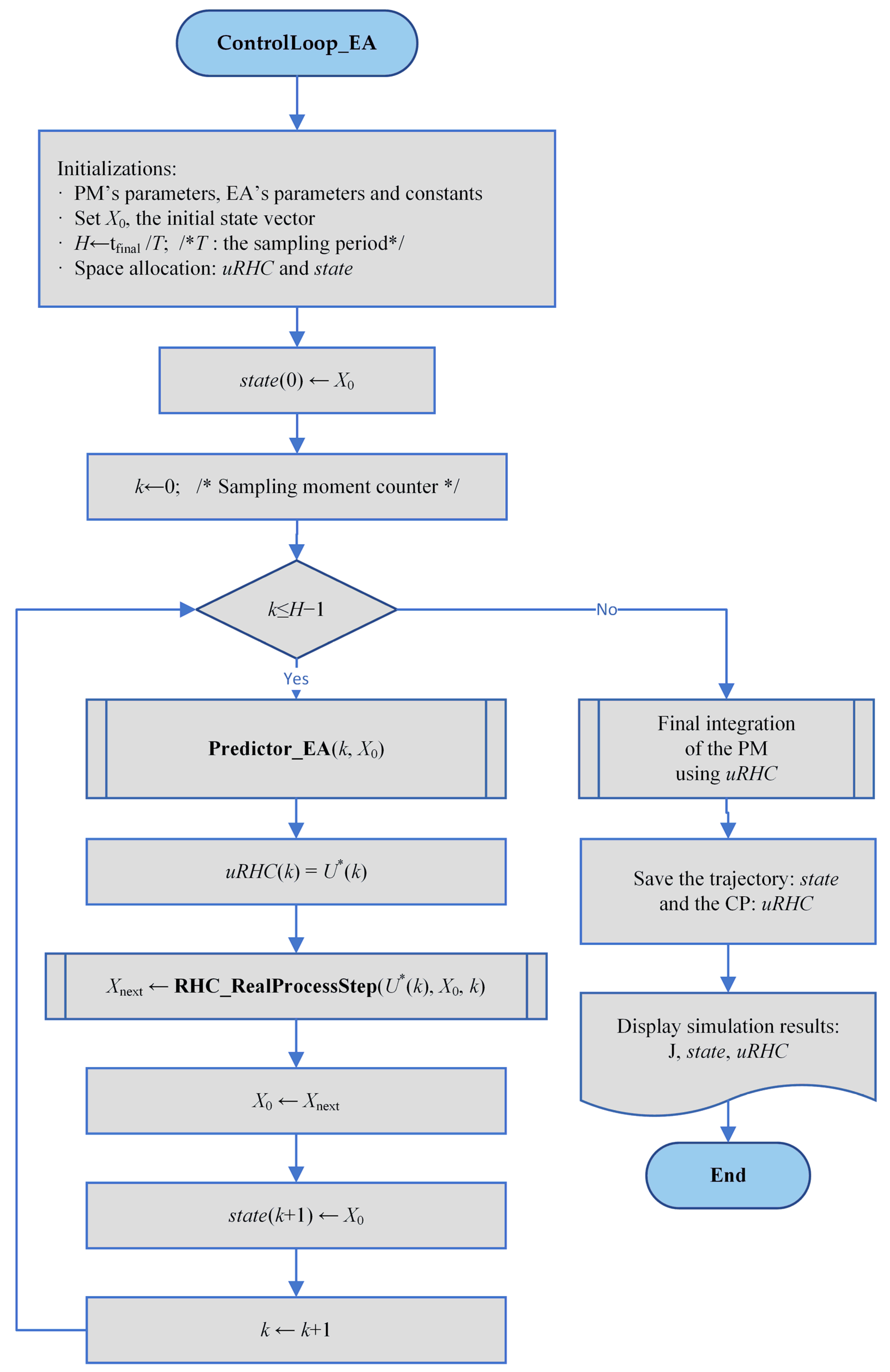
The LOOP_M program calls the ControlLoop_EA program M times to generate training data for the RNN.
Figure A2.
An EA-based algorithm that generates an optimal control profile along with the associated state trajectory.
Appendix D
Data structures representing the optimal trajectories and control profiles yielded by the M executions of the closed-loop simulation program.
Figure A3.
Data structures generated by LOOP_M.m.
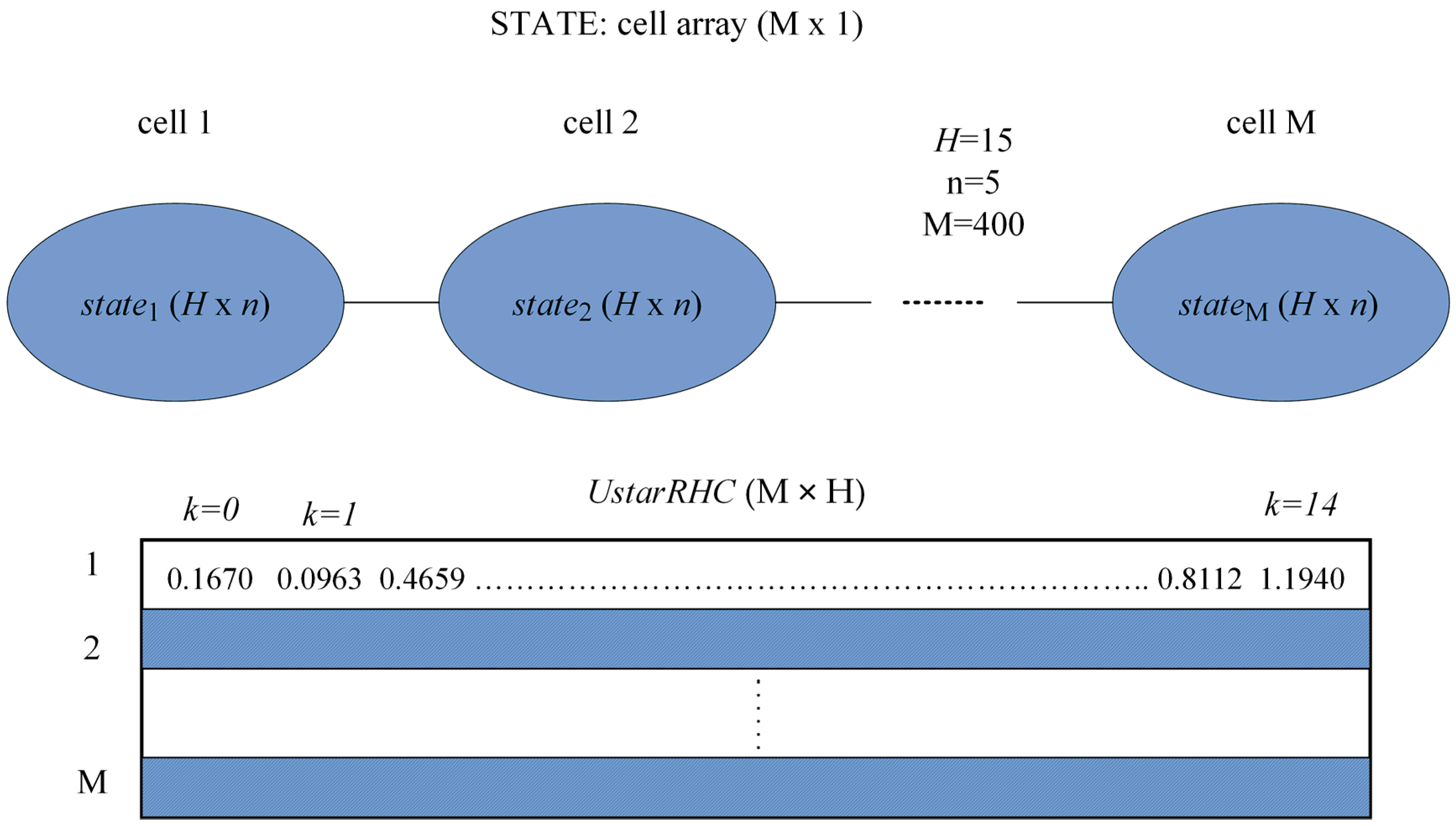
These data structures are used to extract the dataset for each sampling period to train the RNN model. This is a matrix . For example, in the PRP case, for the kth sampling period, it holds:
| Algorithm A1. The training and testing datasets for RNNs at each sampling period | |
| /*This pseudocode prepares the training and testing datasets for each sampling period.*/ Input: STATE cell array (M × 1); UstarRHC matrix (M × H) Output: cell arrays DATAKTrain (H × 1), DATAKTest (H × 1) begin | |
| 1 | for k = 0…H − 1. |
| 2 | for i = 1…M. |
| 3 | |
| 4 | end |
| 5 | #Convert the SOCSK matrix into the datak table. |
| 6 | datakTest60 lines of the datak table |
| 7 | datakTrainThe rest of (M—60) lines of the datak table |
| 8 | DATAKTrain{k}datakTrain |
| 9 | DATAKTest{k}datakTest |
| 10 | end |
| 11 | Save DATAKTrain and DATAKTest in a workspace. |
| end | |
The tables datakTrain and datakTest are extracted from SOCSK.
As a general rule, for each k, 60 random values from column k of the SOCSK matrix were used for the test set, and the remaining values were assigned to the training set. To store these datasets for each k, the cell arrays DATAKTrain and DATAKTest () are used.
Appendix E
Details concerning the use of the scripts, functions, and workspace files, which are materials carried over from [1].
ControlLoop_EA is called M times in LOOP_M.m to generate the training data for the RNN. The LOOP_M script generates the STATE cell array and the UstarRHC matrix, then stores them in the WS_data400.mat workspace. These data encode the M optimal state trajectories and control profiles. The data are described in Appendix D.
The “Cost” and “Next state” functions are important for defining the OCP at hand. The “Next state” functions also achieve the step-by-step numerical integration of the PM. The latter is implemented by the PRProdStep.m function (the PRP’s process in our case).
Most of the OCP’s constraints are implemented in the EA, that is, the script devoted to the predictor.
Appendix E.1. Figure Generation
The closed-loop simulations are performed by the NEW_SIM1, NEW_SIM1_10, and NEW_SIM1_8 scripts. The scripts generate Figure 5, Figure 6 and Figure 7, respectively. After loading the RNN models, these scripts call the NEW_ControlLoop_RNN function. Finally, the NEWDRAW_RNN script draws the two curves.
Figure 4 is generated by the NEW_SIM_EA script, which retrieves the optimal CP and state trajectory from the WS_OPTIMORUM workspace and calls the NEWDRAW_EA script.
Appendix E.2. Execution Time
The processor used for simulations is Intel(R) Core(TM) i7-6700HQ CPU @ 2.60 GHz.
The execution time is a stochastic variable. The statistics for the 6 controllers in Table 7 are generated by the NEW_SIM1_TIME, NEW_SIM1_TIME8, and NEW_SIM1_TIME10 scripts, respectively. The execution time for the controller with multilinear regression functions is taken from [1].
All the above-mentioned scripts, functions, and workspaces are included in the ART_Math folder provided as Supplementary Materials. The folder also includes the “READ ME.pdf” file, which serves as a guide for using the programs.
References
- Minzu, V.; Arama, I. A Machine Learning Algorithm That Experiences the Evolutionary Algorithm’s Predictions—An Application to Optimal Control. Mathematics 2024, 12, 187. [Google Scholar] [CrossRef] [Scilit]
- Siarry, P. Metaheuristics; Springer: Berlin/Heidelberg, Germany, 2016; ISBN 978-3-319-45403-0. [Google Scholar]
- Talbi, E.G. Metaheuristics—From Design to Implementation; Wiley: Hoboken, NJ, USA, 2009; ISBN 978-0-470-27858-1. [Google Scholar]
- Kruse, R.; Borgelt, C.; Braune, C.; Mostaghim, S.; Steinbrecher, M. Computational Intelligence—A Methodological Introduction, 3rd ed.; Springer: Berlin/Heidelberg, Germany, 2022. [Google Scholar] [CrossRef] [Scilit]
- Faber, R.; Jockenhövelb, T.; Tsatsaronis, G. Dynamic optimization with simulated annealing. Comput. Chem. Eng. 2005, 29, 273–290. [Google Scholar] [CrossRef] [Scilit]
- Onwubolu, G.; Babu, B.V. New Optimization Techniques in Engineering; Springer: Berlin/Heidelberg, Germany, 2004. [Google Scholar]
- Valadi, J.; Siarry, P. Applications of Metaheuristics in Process Engineering; Springer: Berlin/Heidelberg, Germany, 2014; pp. 1–39. [Google Scholar] [CrossRef] [Scilit]
- Abraham, A.; Jain, L.; Goldberg, R. Evolutionary Multiobjective Optimization—Theoretical Advances and Applications; Springer: Berlin/Heidelberg, Germany, 2005; ISBN 1-85233-787-7. [Google Scholar]
- Minzu, V.; Serbencu, A. Systematic procedure for optimal controller implementation using metaheuristic algorithms. Intell. Autom. Soft Comput. 2020, 26, 663–677. [Google Scholar] [CrossRef] [Scilit]
- Minzu, V.; Ifrim, G.; Arama, I. Control of Microalgae Growth in Artificially Lighted Photobioreactors Using Metaheuristic-Based Predictions. Sensors 2021, 21, 8065. [Google Scholar] [CrossRef] [Scilit] [PubMed]
- Minzu, V.; Arama, I. Optimal Control Systems Using Evolutionary Algorithm-Control Input Range Estimation. Automation 2022, 3, 95–115. [Google Scholar] [CrossRef] [Scilit]
- Minzu, V.; Georgescu, L.; Rusu, E. Predictions Based on Evolutionary Algorithms Using Predefined Control Profiles. Electronics 2022, 11, 1682. [Google Scholar] [CrossRef] [Scilit]
- Goodfellow, I.; Bengio, Y.; Courville, A. Machine Learning Basics. In Deep Learning; The MIT Press: Cambridge, MA, USA, 2016; pp. 95–161. ISBN 978-0262035613. [Google Scholar]
- Zou, S.; Chu, C.; Shen, N.; Ren, J. Healthcare Cost Prediction Based on Hybrid Machine Learning Algorithms. Mathematics 2023, 11, 4778. [Google Scholar] [CrossRef] [Scilit]
- Cuadrado, D.; Valls, A.; Riaño, D. Predicting Intensive Care Unit Patients’ Discharge Date with a Hybrid Machine Learning Model That Combines Length of Stay and Days to Discharge. Mathematics 2023, 11, 4773. [Google Scholar] [CrossRef] [Scilit]
- Albahli, S.; Irtaza, A.; Nazir, T.; Mehmood, A.; Alkhalifah, A.; Albattah, W. A Machine Learning Method for Prediction of the Stock Market Using Real-Time Twitter Data. Electronics 2022, 11, 3414. [Google Scholar] [CrossRef] [Scilit]
- Newbold, P.; Carlson, W.L.; Thorne, B. Multiple Regression. In Statistics for Business and Economics, 6th ed.; Pfaltzgraff, M., Bradley, A., Eds.; Pearson Education, Inc.: Upper Saddle River, NJ, USA, 2007; pp. 454–537. [Google Scholar]
- Shi, H.; Zhang, X.; Gao, Y.; Wang, S.; Ning, Y. Robust Total Least Squares Estimation Method for Uncertain Linear Regression Model. Mathematics 2023, 11, 4354. [Google Scholar] [CrossRef] [Scilit]
- Goodfellow, I.; Bengio, Y.; Courville, A. Example: Linear Regression. In Deep Learning; The MIT Press: Cambridge, MA, USA, 2016; pp. 104–113. ISBN 978-0262035613. [Google Scholar]
- Hu, X.B.; Chen, W.H. Genetic algorithm based on receding horizon control for arrival sequencing and scheduling. Eng. Appl. Artif. Intell. 2005, 18, 633–642. [Google Scholar] [CrossRef] [Scilit]
- Hu, X.B.; Chen, W.H. Genetic algorithm based on receding horizon control for real-time implementations in dynamic environments. In Proceedings of the 16th Triennial World Congress, Prague, Czech Republic, 4–8 July 2005; Elsevier IFAC Publications: Amsterdam, The Netherlands, 2005. [Google Scholar]
- Mayne, D.Q.; Michalska, H. Receding Horizon Control of Nonlinear Systems. IEEE Trans. Autom. Control. 1990, 35, 814–824. [Google Scholar] [CrossRef] [Scilit]
- Goggos, V.; King, R.E. Evolutionary predictive control. Comput. Chem. Eng. 1996, 20, S817–S822. [Google Scholar] [CrossRef] [Scilit]
- Chiang, P.-K.; Willems, P. Combine Evolutionary Optimization with Model Predictive Control in Real-Time Flood Control of a River System. Water Resour. Manag. 2015, 29, 2527–2542. [Google Scholar] [CrossRef] [Scilit]
- Banga, J.R.; Balsa-Canto, E.; Moles, C.G.; Alonso, A. Dynamic optimization of bioprocesses: Efficient and robust numerical strategies. J. Biotechnol. 2005, 117, 407–419. [Google Scholar] [CrossRef] [Scilit] [PubMed]
- Balsa-Canto, E.; Banga, J.R.; Aloso, A.; Vassiliadis, V. Dynamic optimization of chemical and biochemical processes using restricted second-order information. Comput. Chem. Eng. 2001, 25, 539–546. [Google Scholar] [CrossRef] [Scilit]
- Arama, I.; Mînzu, V. Regression Neural Networks for Emulating Evolutionary Algorithm Predictions in Optimal Control. Open J. Optim. 2026, 15, 23–49. [Google Scholar] [CrossRef]
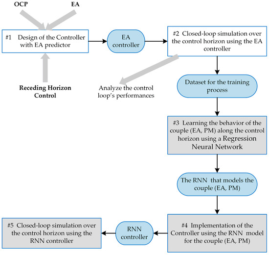
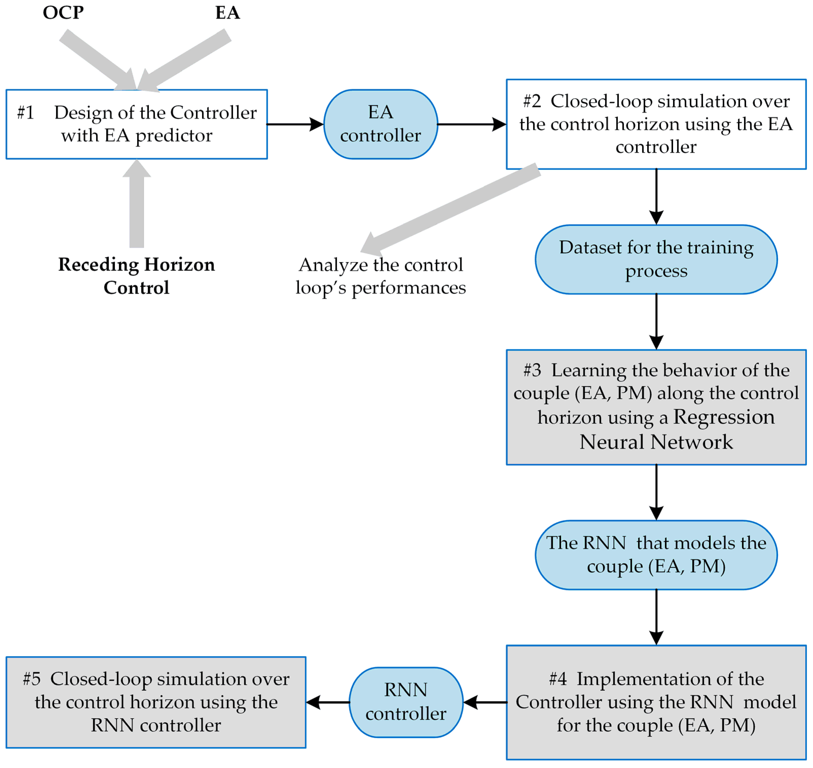
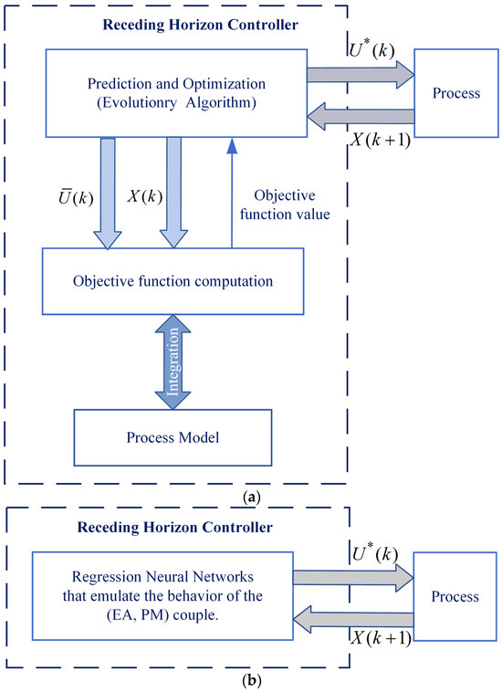
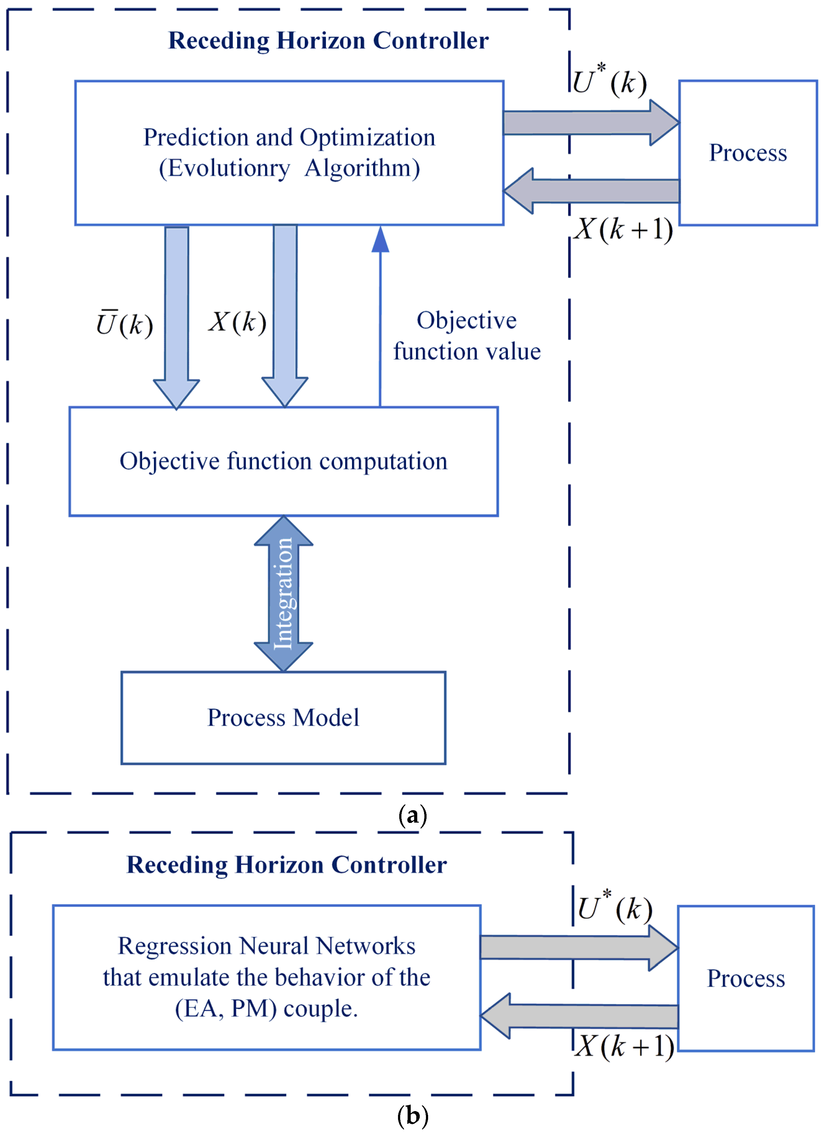


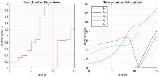
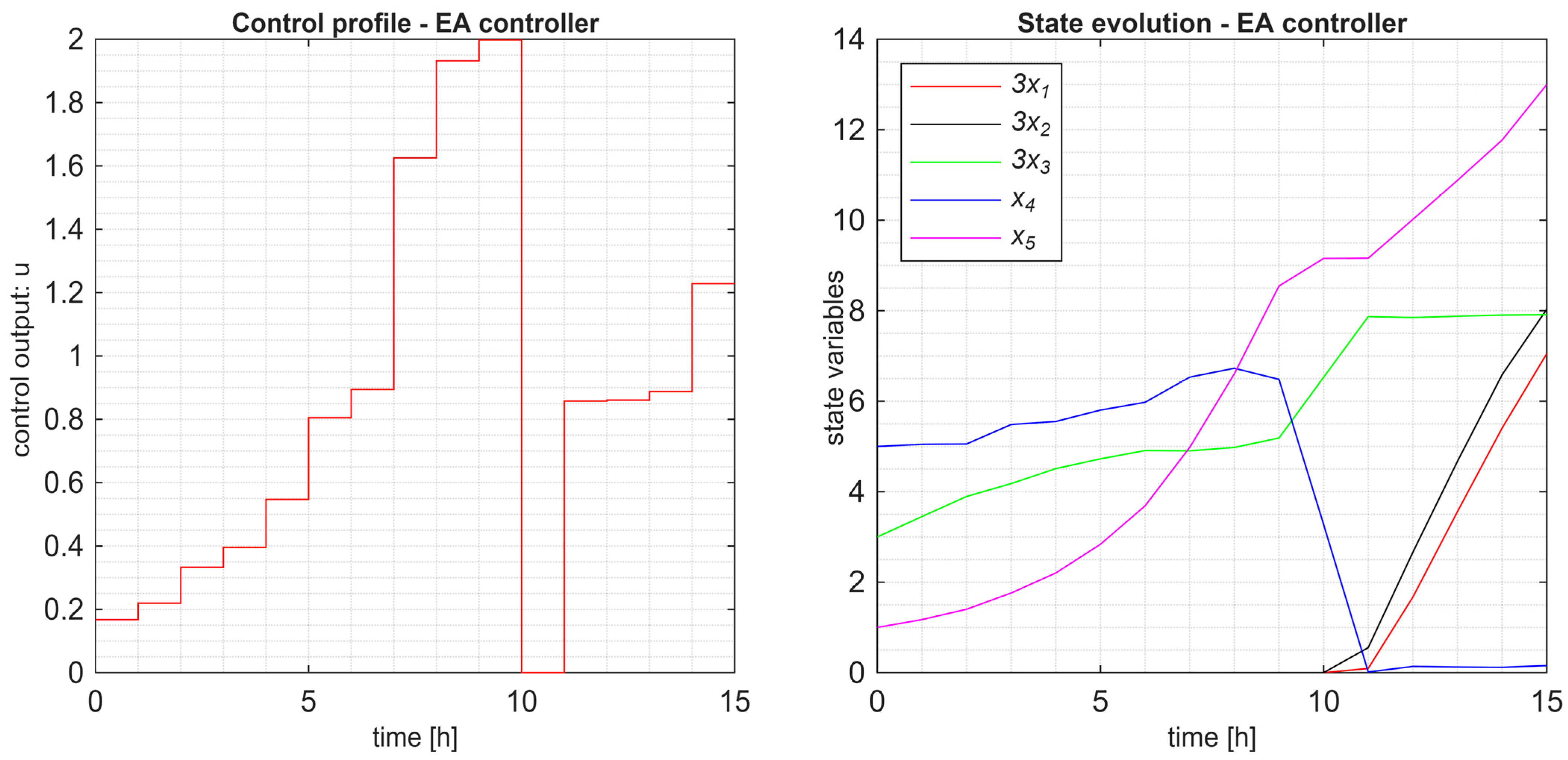
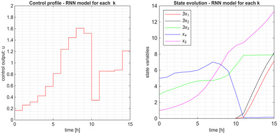
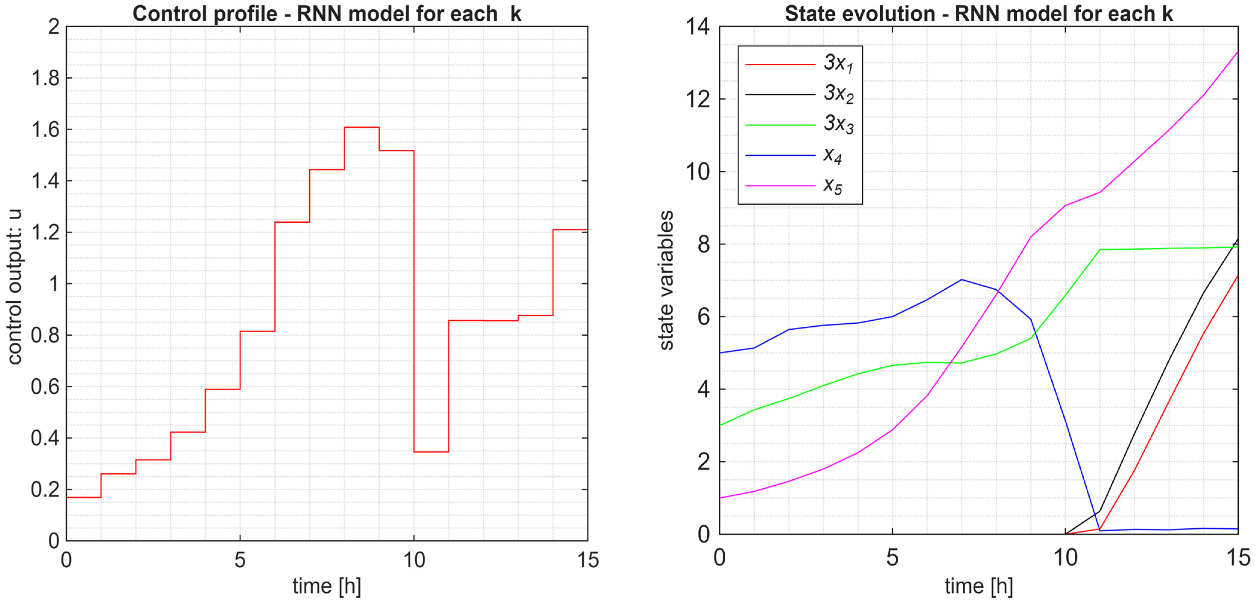
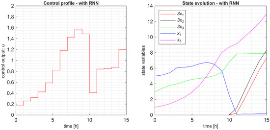
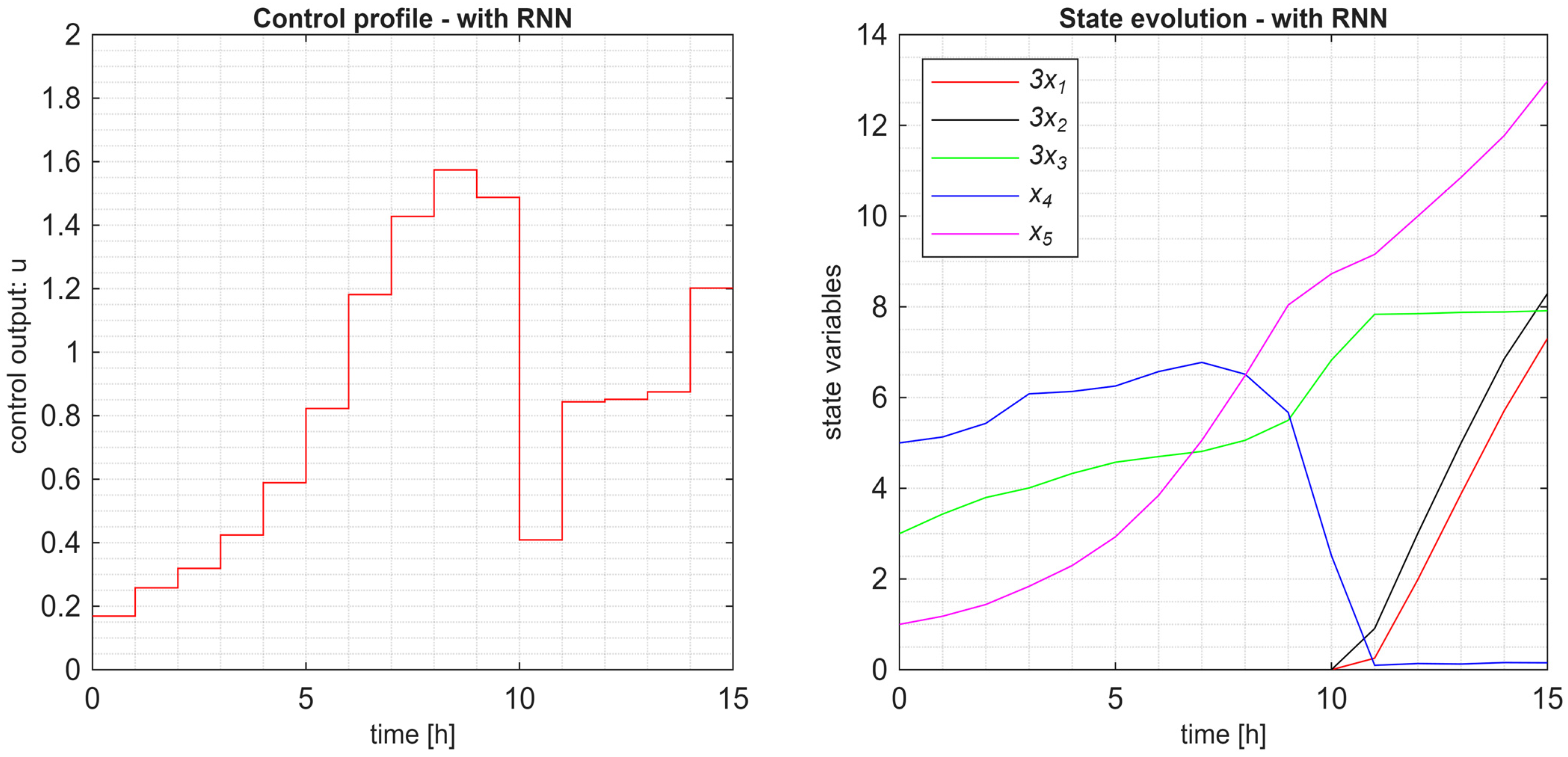
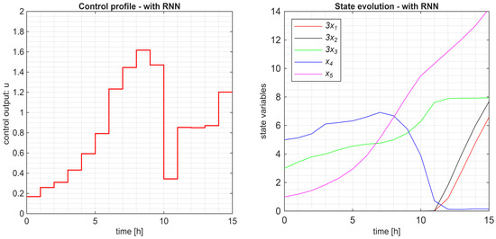
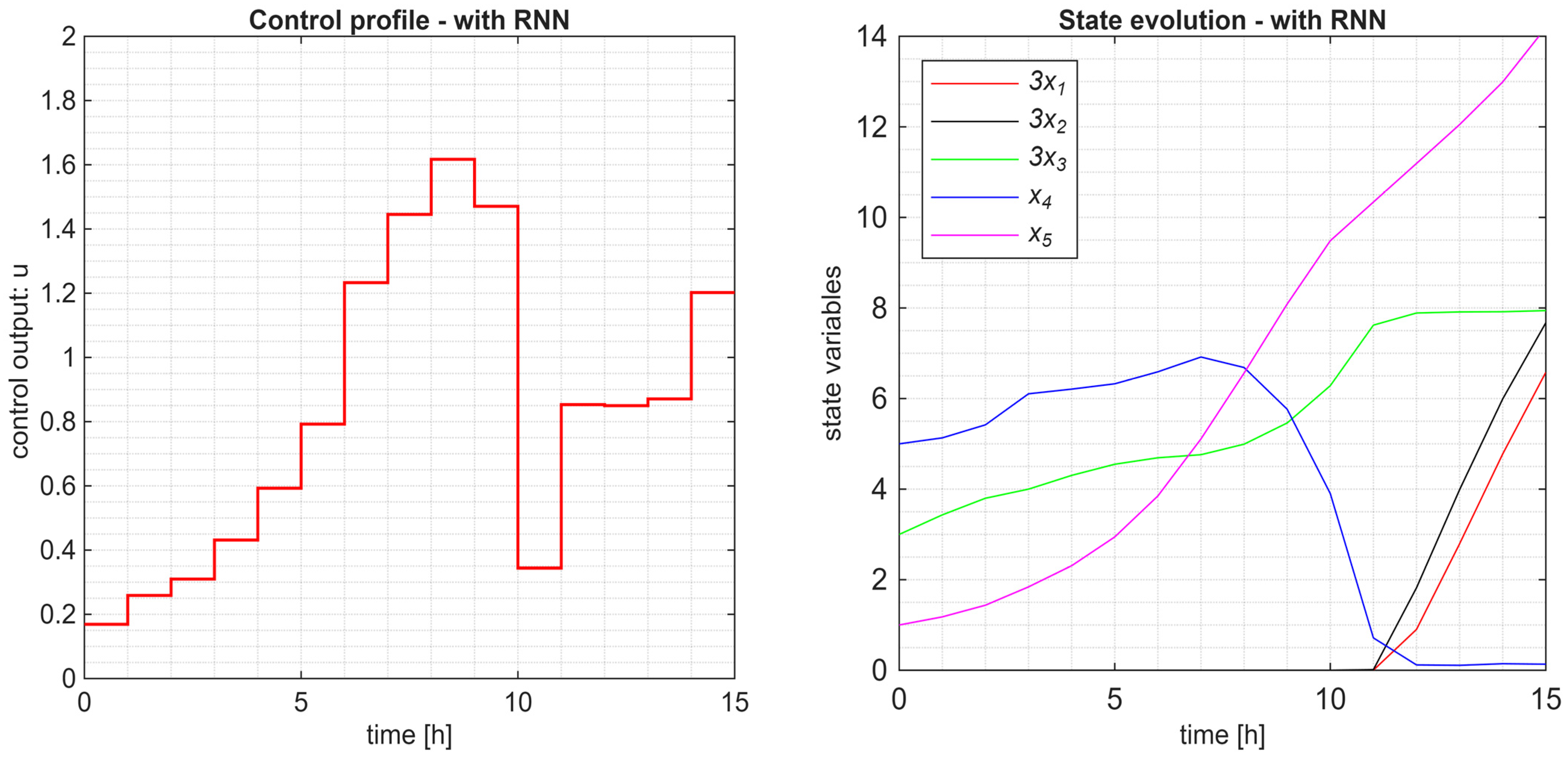
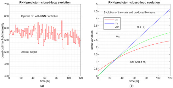
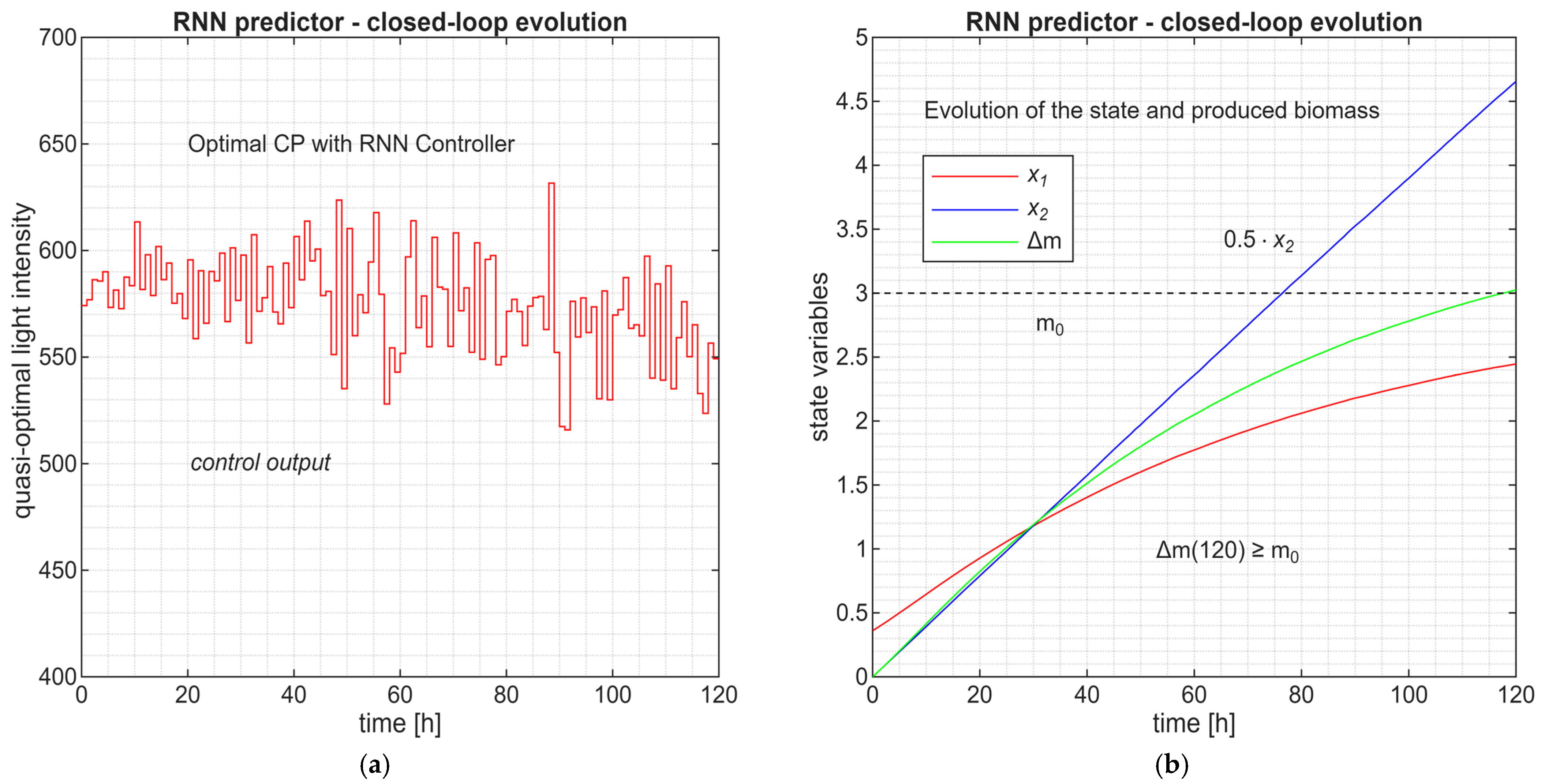
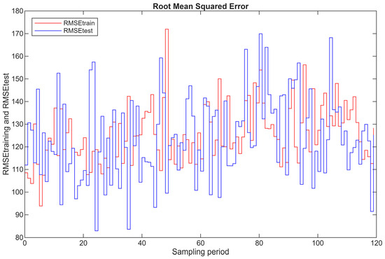
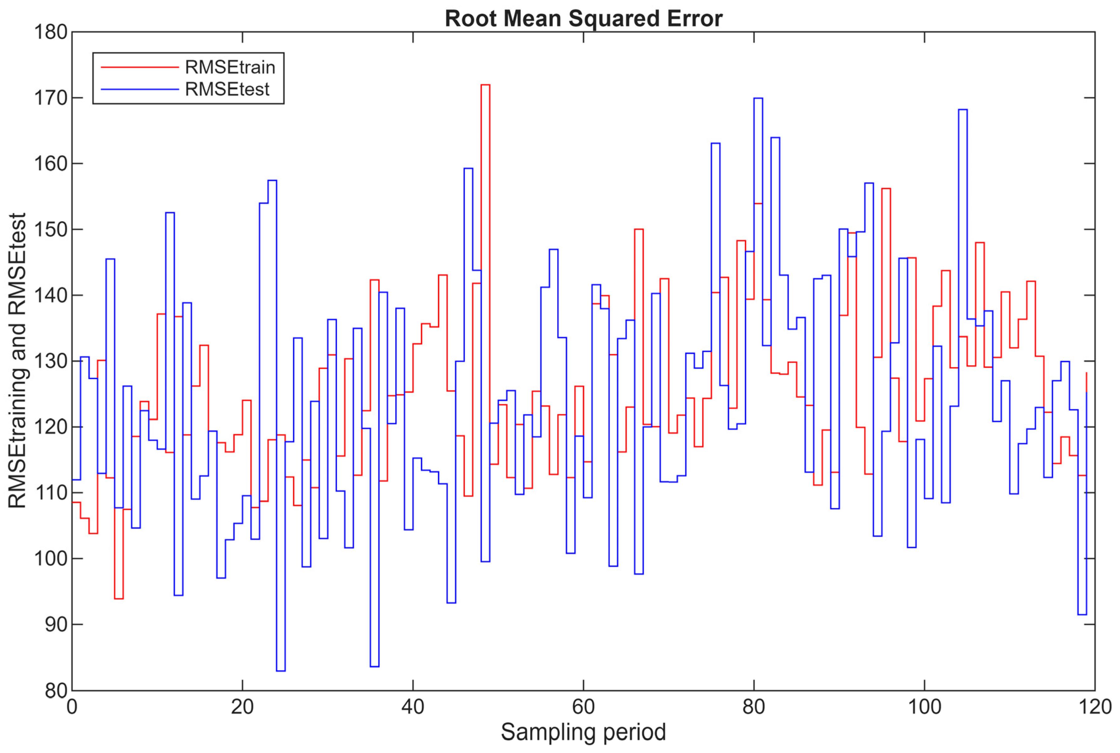

Disclaimer/Publisher’s Note: The statements, opinions and data contained in all publications are solely those of the individual author(s) and contributor(s) and not of MDPI and/or the editor(s). MDPI and/or the editor(s) disclaim responsibility for any injury to people or property resulting from any ideas, methods, instructions or products referred to in the content. |
© 2026 by the authors. Licensee MDPI, Basel, Switzerland. This article is an open access article distributed under the terms and conditions of the Creative Commons Attribution (CC BY) license.