Time-Adaptive Simulated Annealing with Exact-Window Optimization for the Single-Row Facility Layout Problem

Abstract

The single-row facility layout problem (SRFLP) orders unequal-length facilities on a line to minimize flow-weighted center distances. We present a time-adaptive multi-start simulated annealing (AMSA) framework that coordinates one spectral start, randomized restarts, incremental insertion and interchange moves, variable-neighborhood descent (VND), and exact fixed-exterior window optimization under a shared deadline. The primary experiment comprised 137 public instances with 8–1000 facilities and ten fixed seeds per instance, giving 1370 successful runs. Among 133 instances with traceable historical reference values, the best of ten runs reached or improved the study reference on 91 instances. The mean run-level relative gap was 0.00470%, and 57 instances produced the same objective for every seed. New controlled experiments compare six variants on 21 representative instances, nine parameter groups on six instances, serial and concurrent execution on nine instances, and four exclusive runtime stages on nine instances. Full AMSA had the best aggregate rank; only removal of adaptive time allocation differed significantly from the full method after Holm correction. All tested non-default parameter levels had paired Wilcoxon $p>0.05$. Profiling showed that annealing consumed 70.29%, 88.52%, and 96.69% of solver time in the small–medium, medium, and large groups, respectively. Two stored layouts below the archived reference snapshot were independently recomputed by two objective identities with zero discrepancy. These results support AMSA as a reproducible deadline-aware baseline; they do not establish superiority over recent methods evaluated on different platforms or budgets.

1. Introduction

The single-row facility layout problem (SRFLP) is a classical permutation-optimization problem in which facilities of prescribed lengths are arranged without gaps along a line. Its objective is to minimize the sum of pairwise flow coefficients multiplied by the center-to-center distances between facilities. This model captures machine sequencing, storage and service layouts, office allocation, and other one-dimensional material-flow systems [1,2,3]. Although a permutation uniquely determines the resulting geometry, the search space contains $n!$ layouts, making exact optimization rapidly intractable as the number of facilities increases.

Exact approaches based on mixed-integer, semidefinite, cutting-plane, and polyhedral formulations have produced strong bounds and certified solutions for small and medium-sized instances [4,5,6]. As the problem size grows, however, SRFLPs are more commonly tackled with fast local-search procedures and metaheuristics. Representative methods include insertion-based Lin–Kernighan search, tabu and scatter search, GRASP, variable-neighborhood search, genetic algorithms, and simulated annealing [7,8,9]. In particular, Palubeckis [10] developed a multi-start simulated-annealing (MSA) algorithm with linear-time insertion and interchange-gain evaluation and reported results for instances with up to 1000 facilities.

Recent studies have raised the quality standard considerably. Tang et al. [11] introduced the K-medoids memetic permutation-group (KMPG) algorithm, which combines permutation-group symmetry breaking, clustering-guided crossover, simulated-annealing improvement, and population management. Chen et al. [12] proposed an oscillation-based simulated-annealing method that alternates between two search regimes and reported improved upper bounds on a broad test set. Pammer and Sinnl [13] incorporated exact-window optimization with a fixed exterior into a matheuristic and likewise obtained new bounds. Together, these results indicate that high-quality SRFLP algorithms must balance global structural diversification with strong local intensification. They also underscore the need for disciplined comparisons: reaching an older best-known value on a different machine or under a different time budget is not, by itself, evidence of state-of-the-art performance.

This study addresses a complementary question: how can a compact, single-threaded MSA implementation use a user-specified wall-clock budget effectively across a wide range of instance sizes? In a time-limited annealing run, the temperature scale, trials per level, stagnation detection, restart duration, and final intensification all compete for the same finite budget. If the initial temperature is estimated from an extreme sampled gain, short runs may spend too long in an unproductive high-temperature phase. Conversely, devoting nearly the entire budget to a single locally converged trajectory limits global coverage. Exact-window optimization is beneficial only when time is explicitly reserved for it and when it is applied to a sufficiently strong incumbent.

We address these interactions with a time- and size-adaptive search portfolio. The first restart is initialized by a flow-graph spectral ordering, whereas subsequent restarts preserve stochastic diversity. Simulated annealing calibrates its temperature from sampled uphill gains and a target acceptance probability; insertion–interchange variable-neighborhood descent (VND) then provides deterministic intensification. Exact-window optimization uses subset dynamic programming while fixing the external order. All stages obey a shared hard deadline, and every global-incumbent update is checked by full objective recomputation.

The contributions of this study are as follows:

• A deadline-aware coordination policy that protects a final-intensification reserve and allocates size- and time-dependent restart budgets across otherwise established search modules.
• An incremental, cut-based implementation for insertion and interchange moves, supported by randomized differential tests against full objective recomputation.
• A scale-adaptive parameterization in which neighborhood radii, temperature levels, stagnation limits, restart budgets, and the final reserve depend on n and the requested time budget.
• A reproducible 137-instance study accompanied by a same-platform conventional MSA baseline and controlled six-variant ablation on representative instances.
• Paired parameter-sensitivity, concurrency, runtime-decomposition, and independent candidate-permutation audits, with complete run-level evidence.

We interpret the computational evidence conservatively. Matching a published reference value means that the target was reached; it does not establish global optimality unless that target is certified. Two values improve the 2023-era reference table used in our analysis, but we present them as candidate improvements pending comparison with the newer 2025–2026 result repositories. Without runs conducted on matched hardware and under equal stopping budgets, we make no superiority claim over KMPG, oscillation-based simulated annealing, or the recent matheuristic.

The remainder of this paper is organized as follows. Section 2 reviews exact, heuristic, and recent hybrid approaches. Section 3 formulates the SRFLP. Section 4 describes the algorithm, implementation checks, and experimental protocol. Section 5 presents the results, Section 6 discusses their interpretation and limitations, and Section 7 concludes the study.

2. Related Work

2.1. Exact Models and Bounds

Early mathematical treatments represented one-dimensional allocation through integer or ordering formulations [2,3]. Subsequent studies strengthened exact solution through semidefinite relaxations, cutting planes, lower bounds, and polyhedral analysis [4,5,6,14,15]. Computational reviews show that these methods can certify or tightly bound increasingly large instances, although their computational requirements grow rapidly [16,17].

2.2. Heuristics and Metaheuristics

Heuristic SRFLP research has explored complementary search paradigms. Simulated-annealing studies examined temperature and neighborhood choices for single-row layouts [18]. Later work developed tabu search, permutation-based genetic search, insertion-based Lin–Kernighan improvement, hybrid genetic algorithms, and combined variable-neighborhood and ant-colony search [7,8,19,20,21]. Palubeckis [10] combined multi-start simulated annealing with fast move evaluation for instances containing up to 1000 facilities, while Cravo and Amaral [9] proposed a GRASP method for large-scale cases.

2.3. Recent Hybrid Methods and Research Positioning

Recent methods place greater emphasis on coordinating global diversity with strong local improvement. Wang and Xu [22] proposed a compact functionalized memetic algorithm. Tang et al. [11] combined permutation-group symmetry handling, clustering-guided crossover, simulated-annealing improvement, and population management. Chen et al. [12] developed an oscillation-based simulated annealer, whereas Pammer and Sinnl [13] embedded exact-window optimization with a fixed exterior within a matheuristic. Because these studies used different hardware and stopping conditions, the present work reports reference attainment and distributional behavior rather than claiming an unmatched algorithm ranking.

Spectral seriation, multi-start simulated annealing, incremental move evaluation, VND, and fixed-exterior exact-window optimization all have clear precedents. We therefore do not claim any of these modules individually as a new algorithm. The specific methodological contribution is their deadline-aware coordination: a common steady-clock deadline, a size- and budget-dependent restart horizon, and a protected final reserve that earlier trajectories cannot consume. The experimental contribution is a reproducible multi-seed evaluation that explicitly tests this coordination against module-removal variants and a conventional MSA baseline.

3. Problem Formulation

Let $\mathcal{N}=\{1,\dots ,n\}$ be the facility set. Facility i has length $l_i>0$, and $w_{ij}\ge 0$ denotes the interaction coefficient between facilities i and j. A solution is a permutation $\pi =\left(\pi \right(1),\dots ,\pi (n\left)\right)$. Under contiguous placement, the center coordinate of the facility at position k is

$$x_{\pi \left(k\right)}={\displaystyle \sum _{h=1}^{k-1}}{l}_{\pi \left(h\right)}+{\displaystyle \frac{l_{\pi \left(k\right)}}{2}}$$

(1)

The objective is

$$F\left(\pi \right)=\sum _{1\le k<q\le n}{w}_{\pi \left(k\right),\pi \left(q\right)}\left|x_{\pi \left(k\right)}-x_{\pi \left(q\right)}\right|$$

(2)

For directed-flow files, distance symmetry permits aggregation into an undirected coefficient $w_{ij}^{\prime }=w_{ij}+w_{ji}$. Files that already contain a symmetric pair coefficient are retained unchanged. Diagonal terms make no contribution. Internally, lengths and center distances are doubled so that intermediate geometric quantities remain integral; the final objective is divided by two. Hence, half-integral objective values are valid.

4. Materials and Methods

4.1. Conventional Multi-Start Simulated Annealing Baseline

The conventional baseline uses the same instance parser, objective function, insertion and interchange move evaluators, pseudo-random generator, seeds, wall-clock limits, and output validation as AMSA. Each trajectory begins from a uniformly shuffled permutation. At every temperature, it samples insertion or interchange moves, accepts improving moves unconditionally, and accepts a worsening move of cost increase $\Delta >0$ with probability $\exp (-\Delta /T)$. The temperature follows the same geometric cooling rule, and the best solution observed across trajectories is returned at interruption. The baseline excludes spectral initialization, VND, exact-window optimization, and the adaptive restart/final-reserve policy.

Simulated annealing was selected as the host metaheuristic because its Metropolis rule permits controlled escape from local optima in permutation space, its incumbent is available at any interruption point, and its trajectory naturally fits a wall-clock stopping condition. It also provides a direct conventional comparator for the proposed coordination policy. This choice does not imply that SA dominates genetic, tabu, ant-colony, or other metaheuristics; recent methods from those families remain relevant reference comparators when matched implementations and budgets are available.

4.2. Search Architecture

The algorithm maintains a global incumbent and launches successive trajectories until a shared hard deadline; this multi-start structure separates restart-based diversification from local intensification [23]. The first trajectory is initialized by spectral seriation and immediately improved by variable-neighborhood descent (VND). Later trajectories start from uniformly random permutations to avoid excessive dependence on one constructive rule. Each trajectory applies simulated annealing with insertion and interchange moves, restores its best encountered state, and invokes local search and exact-window optimization when time remains. A final intensification pass applies VND and overlapping exact-window optimization to the global incumbent. Algorithm 1 summarizes the framework.

Algorithm 1 Adaptive Multi-Start Simulated Annealing (AMSA)
1:	Input: interaction matrix W, facility lengths l, and deadline d
2:	Output: best permutation ${\pi }^{*}$ and objective value $F^{*}$
3:	$F^{*}\leftarrow +\infty$; $r\leftarrow 0$;
4:	while time remains before d do
5:	if $r=0$ then
6:	$\pi \leftarrow \mathrm{SpectralOrder}\left(W\right)$; $\pi \leftarrow \mathrm{VND}\left(\pi \right)$;
7:	else
8:	draw a uniformly random permutation $\pi$;
9:	end if
10:	initialize incremental cut data and estimate $T_0$ from sampled uphill gains;
11:	$\pi \leftarrow \mathrm{SimulatedAnnealing}(\pi ,T_0,d)$; $\pi \leftarrow \mathrm{VND}\left(\pi \right)$;
12:	if $F\left(\pi \right)\le 1.00010F^{*}$ then
13:	$\pi \leftarrow \mathrm{ExactWindowDP}\left(\pi \right)$;
14:	end if
15:	update $({\pi }^{*},F^{*})$ if $\pi$ improves the global incumbent;
16:	$r\leftarrow r+1$;
17:	end while
18:	apply VND and two overlapping exact-window optimization passes to ${\pi }^{*}$;
19:	return$({\pi }^{*},F^{*})$

4.3. Spectral Initialization

Let $d_i={\sum }_{j=1}^n{w}_{ij}$, $D=\mathrm{diag}(d_1,\dots ,d_n)$, and $L=D-W$ be the weighted graph Laplacian. Motivated by Fiedler-vector ordering and spectral seriation [24,25], the implementation uses a projected power iteration as a structure-aware initialization heuristic. Projected iteration was chosen instead of forming a dense eigendecomposition because it requires only repeated matrix–vector products, has deterministic memory use, and can be truncated after a small prescribed iteration count under short deadlines. A direct sparse eigensolver could be more accurate, but would introduce library-, tolerance-, and convergence-dependent overhead that is disproportionate for the single seeded trajectory. Define $d_{\max }=\max (1,{\max }_i{d}_i)$, $\alpha =0.9/d_{\max }$, and $I_s=\mathrm{clamp}(60+\lfloor n/2\rfloor ,80,250)$. The initial entries $x_i^{\left(0\right)}$ are drawn from $[-0.5,0.5)$ by the study’s seeded pseudo-random generator. At iteration r, the update is

$$y^{(r+1)}=(I-\alpha L)x^{\left(r\right)},{\tilde{y}}^{(r+1)}=y^{(r+1)}-{\displaystyle \frac{{\mathbf{1}}^{\mathsf{T}}{y}^{(r+1)}}{n}}\mathbf{1}$$

(3)

followed by

$$x^{(r+1)}={\displaystyle \frac{{\tilde{y}}^{(r+1)}}{\sqrt{\max (\parallel {\tilde{y}}^{(r+1)}{\parallel }_2^2,{10}^{-30})}}}$$

(4)

After $I_s$ iterations, facilities are stably sorted by increasing $x_i^{\left(I_s\right)}$; equal values retain increasing facility index. The sign ambiguity of a spectral vector only reverses the order, which leaves the SRFLP objective unchanged. Exactly one trajectory per run uses this spectral ordering; every later restart is a uniformly shuffled permutation. For a graph containing two disconnected components, the zero eigenvalue is repeated and the relative component placement is not uniquely determined. The seeded starting vector and stable facility-index tie rule then select one reproducible component ordering, after which VND may rearrange it. The same interpretation applies when symmetric components create a repeated Fiedler eigenvalue: the result is a seeded seriation heuristic, not a unique eigenvector or an optimality certificate. Algorithm 2 gives the implemented steps.

Algorithm 2 Projected spectral initialization
1:	Input: symmetric interaction matrix W and pseudo-random seed z
2:	Output: spectral starting permutation ${\pi }^{\mathrm{sp}}$
3:	compute $d_i\leftarrow {\sum }_j{w}_{ij}$, $d_{\max }\leftarrow \max (1,{\max }_i{d}_i)$, and $\alpha \leftarrow 0.9/d_{\max }$;
4:	set $I_s\leftarrow \mathrm{clamp}(60+\lfloor n/2\rfloor ,80,250)$ and draw $x_i\sim U[-0.5,0.5)$ using z;
5:	for  $r=0,\dots ,I_s-1$  do
6:	$y\leftarrow x-\alpha (D-W)x$;
7:	$y\leftarrow y-({\mathbf{1}}^{\mathsf{T}}y/n)\mathbf{1}$;
8:	$x\leftarrow y/\sqrt{\max (\parallel y{\parallel }_2^2,{10}^{-30})}$;
9:	end for
10:	stably sort facility indices by increasing $x_i$ to obtain ${\pi }^{\mathrm{sp}}$;
11:	return  ${\pi }^{\mathrm{sp}}$

4.4. Incremental Move Evaluation

The implementation uses a cut representation. After directed flows have been aggregated into the symmetric coefficients described in Section 3, the interaction crossing the boundary between positions t and $t+1$ is

$$c_t\left(\pi \right)={\displaystyle \sum _{p=1}^t}{\displaystyle \sum _{q=t+1}^n}{w}_{\pi \left(p\right),\pi \left(q\right)}$$

(5)

The distance between two facility centers equals one half of the sum of the adjacent facility-length pairs across the intervening boundaries. Interchanging the order of summation therefore gives

$$2F\left(\pi \right)={\displaystyle \sum _{t=1}^{n-1}}{c}_t\left(l_{\pi \left(t\right)}+l_{\pi (t+1)}\right)$$

(6)

An insertion or interchange with endpoints i and j changes only the facility order and cut values on the boundaries spanned by those endpoints. The implementation subtracts the old terms and adds the new terms from Equation (6) using 64-bit integer arithmetic. Evaluating and applying either move consequently requires $O\left(\right|i-j\left|\right)$ time and $O\left(1\right)$ auxiliary storage, rather than an $O\left(n^2\right)$ complete objective recomputation. The inverse position map and affected cut values are updated after every accepted move; randomized differential tests then compare the accumulated gain with a complete evaluation of Equation (2).

4.5. Temperature and Acceptance

Following the standard acceptance-based formulation of simulated annealing [26,27], let ${\overline{\Delta }}^{+}$ denote the mean positive interchange cost increase in a preliminary sample. The implementation uses $m_T=\min (5000,\max (100,10n))$ sampled moves and target acceptance probability $P_0=0.8$. If the sample contains at least one positive gain, the initial temperature is

$$T_0=\max \left(1,{\displaystyle \frac{{\overline{\Delta }}^{+}}{-\ln P_0}}\right)$$

(7)

and $T_0=1$ if no sampled gain is positive. At temperature T, a move with gain $\Delta$ is accepted when $\Delta \le 0$; otherwise, it is accepted with probability $\exp (-\Delta /T)$. Let $L_T=\mathrm{clamp}(35+\lfloor n/8\rfloor ,45,120)$ be the target cooling horizon and $T_{\min }={10}^{-4}$. The geometric factor used by the code is

$$\rho =\mathrm{clamp}({\rho }_0,0.82,0.96),{\rho }_0={\left({\displaystyle \frac{\max (T_{\min },1)}{\max (T_0,1)}}\right)}^{1/L_T}$$

(8)

The value $L_T$ parameterizes the cooling rate; it is not an additional stopping limit. Each level samples $M=\max (200,20n)$ moves unless the user supplies an override. Interchanges are selected with probability 0.35 and insertions otherwise. A trajectory stops when $T\le T_{\min }$, when $S=\mathrm{clamp}(12+\lfloor n/40\rfloor ,12,30)$ consecutive levels fail to improve the trajectory best, or when its deadline is reached.

Algorithm 3 makes explicit the control flow implemented for one annealing trajectory. In particular, the incumbent of a trajectory is stored separately from its current state, so accepted uphill moves cannot overwrite the best solution found by that restart.

Algorithm 3 One adaptive simulated-annealing trajectory
1:	Input: permutation $\pi$, deadline d, and target acceptance probability $P_0$
2:	Output: best state ${\pi }^b$ found by the trajectory
3:	${\pi }^b\leftarrow \pi$; initialize the cut array;
4:	sample $m_T$ interchange gains and compute $T_0$, $L_T$, $\rho$, and stagnation limit S;
5:	$T\leftarrow T_0$; $s\leftarrow 0$;
6:	while $T>T_{\min }$, $s<S$, and time is before d do
7:	$improved\leftarrow \mathbf{false}$;
8:	for $m=1,\dots ,M$ while time is before d do
9:	select interchange with probability $0.35$ and insertion otherwise; evaluate $\Delta$;
10:	if $\Delta \le 0$ or $U(0,1)<\exp (-\Delta /T)$ then
11:	apply the move and update the inverse positions and affected cuts;
12:	if $F\left(\pi \right)<F\left({\pi }^b\right)$ then
13:	${\pi }^b\leftarrow \pi$; $improved\leftarrow \mathbf{true}$;
14:	end if
15:	end if
16:	end for
17:	if $improved$ then $s\leftarrow 0$; else $s\leftarrow s+1$; end if
18:	$T\leftarrow \rho T$;
19:	end while
20:	$\pi \leftarrow {\pi }^b$;
21:	return  ${\pi }^b$

4.6. Variable-Neighborhood Descent

Following the neighborhood-change principle of variable-neighborhood search [28], the VND alternates best-improvement insertion and interchange scans. For $n\le 250$, complete neighborhoods are scanned. For larger instances, the radius is $\mathrm{clamp}(n/10,5,50)$. The search first descends to an insertion local optimum; it then applies the best improving interchange and returns to insertion search. This cycle terminates when neither neighborhood improves the current layout, the move limit is reached, or the deadline expires.

4.7. Exact-Window Optimization

A contiguous window of at most 14 facilities is optimized exactly while the order outside the window is fixed. In the spirit of subset dynamic programming and dynamically searched large neighborhoods [29,30,31], the implementation avoids factorial enumeration. Consider positions $[s,e]$, let $Q=\left\{\pi \right(s),\dots ,\pi (e\left)\right\}$ and $w=\left|Q\right|$, and define $a(u,v)=l_u+l_v$. The facilities in positions smaller than s form the fixed-left set $L_s$. For each $u\in Q$, let

$$g_u={\displaystyle \sum _{v=1}^n}{w}_{uv},b_u=\sum _{v\in L_s}{w}_{uv}$$

(9)

and set $C(⌀)=c_{s-1}$ when $s>1$, with $C(⌀)=0$ when $s=1$. If $S\subseteq Q$ is the set already placed from left to right inside the window, the cut immediately after those facilities is

$$C\left(S\right)=C(⌀)+\sum _{u\in S}(g_u-2b_u)-2\sum _{\begin{array}{c}u,v\in S\\ u<v\end{array}}{w}_{uv}$$

(10)

Equivalently, when $u\notin S$ is appended, $C(S\cup \left\{u\right\})=C\left(S\right)+g_u-2(b_u+{\sum }_{v\in S}{w}_{uv})$. This recurrence is independent of the order used to construct S and incorporates interactions with both fixed sides through the boundary cut.

Let $DP[S,j]$ be the minimum contribution to the doubled objective in Equation (6) among partial window orders containing exactly S and ending at $j\in S$. If $q_L=\pi (s-1)$ exists, the boundary condition is

$$DP[\left\{j\right\},j]=C(⌀)a(q_L,j);$$

(11)

otherwise it is zero. For $k\in Q\setminus S$, the transition is

$$DP[S\cup \left\{k\right\},k]=\underset{j\in S}{\min }\left\{DP[S,j]+C\left(S\right)a(j,k)\right\}$$

(12)

If the fixed-right neighbor $q_R=\pi (e+1)$ exists, the terminal value is

$$G^{*}=\underset{j\in Q}{\min }\left\{DP[Q,j]+C\left(Q\right)a(j,q_R)\right\};$$

(13)

otherwise the terminal boundary term is omitted. The current affected contribution is

$$G_{\mathrm{old}}={\displaystyle \sum _{t=\max (1,s-1)}^{\min (n-1,e)}}{c}_t\left(\pi \right)a(\pi \left(t\right),\pi (t+1))$$

(14)

All terms outside this boundary range are invariant because the external order and the set Q are fixed. Hence, $G^{*}<G_{\mathrm{old}}$ is a sufficient and exact test for strict improvement of the complete SRFLP objective. Predecessor records reconstruct the minimizing window order. The implementation then rebuilds the cut data and recomputes the complete objective before updating the global incumbent. The dynamic program uses $O\left(2^w{w}^2\right)$ time and $O\left(2^{w}w\right)$ memory.

During each restart, one window of length $\min (14,n)$ is placed at a uniformly sampled feasible start only when $F\left(\pi \right)\le 1.00010F^{*}$. Final intensification uses two overlapping passes with stride $\max (1,\lfloor w/2\rfloor )$; the second pass is offset by $\lfloor \mathrm{stride}/2\rfloor$, and a terminal window may be shorter. All passes stop at the shared deadline. This procedure is termed exact-window optimization throughout the paper; “exact” refers only to the fixed-exterior window subproblem, not to global solution of the SRFLP. Algorithm 4 summarizes the fixed-exterior exact-window procedure.

Algorithm 4 Exact-window optimization with a fixed exterior
1:	Input: incumbent $\pi$ and window $[s,e]$ of length $w\le 14$
2:	Output: permutation ${\pi }^{\prime }$ with $F\left({\pi }^{\prime }\right)\le F\left(\pi \right)$
3:	form Q and compute $g_u$, $b_u$, and $C\left(S\right)$ using Equations (9) and (10);
4:	initialize $DP\left[\right\{j\},j]$ by Equation (11) and store predecessor records;
5:	for every nonempty proper subset $S\subset Q$ do
6:	for each $j\in S$ and $k\in Q\setminus S$ do
7:	relax $DP[S\cup \{k\},k]$ by Equation (12);
8:	end for
9:	end for
10:	compute $G^{*}$ and reconstruct the minimizing order; compute $G_{\mathrm{old}}$;
11:	if  $G^{*}<G_{\mathrm{old}}$  then
12:	splice the reconstructed order into $\pi$, rebuild cuts, and recompute $F\left(\pi \right)$;
13:	else
14:	leave $\pi$ unchanged;
15:	end if
16:	return  $\pi$

4.8. Adaptive Controls and Stopping

Let $d_0$ be the steady-clock start and $d=d_0+\tau$ the common hard deadline. The protected final reserve is $R_f=\min (8,\max (0.35,0.20\tau ))$ seconds, so new restarts may begin only before $d_r=d-R_f$. A restart started at time t receives the local endpoint $\min (d_r,t+R_r)$, where $R_r=\min (10,\max (0.35,0.12\tau ))$ seconds. Annealing, within-restart VND, and the triggered window call all obey that endpoint. When $d_r$ is reached, the algorithm restores the global incumbent and spends the still-protected interval on final VND and two overlapping exact-window passes, all bounded by d. Thus, earlier trajectories cannot consume the final reserve. The no-adaptive ablation removes this protection and uses a fixed restart budget.

The scale-adaptive controls are summarized in Table 1.

Table 1. Scale-adaptive controls used in the implementation.

Component	Rule
Neighborhood radius	complete neighborhood for $n\le 250$; otherwise $\mathrm{clamp}(\lfloor n/10\rfloor ,5,50)$
Spectral iterations	$\mathrm{clamp}(60+\lfloor n/2\rfloor ,80,250)$
Temperature sample	$\min (5000,\max (100,10n\left)\right)$ interchange gains
Initial acceptance	$P_0=0.8$; $T_0=1$ if no sampled gain is positive
Minimum temperature	$T_{\min }={10}^{-4}$
Target cooling horizon	$\mathrm{clamp}(35+\lfloor n/8\rfloor ,45,120)$
Trials per level	$\max (200,20n)$ unless overridden
Stagnant levels	$\mathrm{clamp}(12+\lfloor n/40\rfloor ,12,30)$
Restart budget	$\max (0.35,0.12\tau )$, capped at 10 s
Final reserve	$\max (0.35,0.20\tau )$, capped at 8 s
Exact-window length	$\min (14,n)$, with two overlapping final passes

The trigger $F\left(\pi \right)\le 1.00010F^{*}$ is a computational gate, not a theoretical constant: exact-window dynamic programming is reserved for trajectories already within 0.01% of the incumbent. The sensitivity study tests triggers 1.00000, 1.00010, and 1.00050 as well as window lengths 10, 12, and 14.

4.9. Correctness and Reproducibility

All matrices used by the search are symmetric after preprocessing. If any off-diagonal pair differs, the file is treated as directed and the coefficient for unordered pair $\{i,j\}$ is set to $w_{ij}^{\prime }=w_{ij}+w_{ji}$; if the matrix is already symmetric, its pair coefficient is retained once rather than doubled. Diagonal entries are set to zero. A validator checks that every facility appears exactly once and that the inverse position map agrees with the permutation.

For an accepted instance, let $L={\sum }_i{l}_i$ and $W={\sum }_{i<j}{w}_{ij}^{\prime }$. Since every center distance is at most L, the doubled internal objective satisfies $2F\left(\pi \right)\le 2LW$ for every permutation. The revised reader checks doubled lengths, pair aggregation, and doubled pair weights before storing them in 32-bit arrays; it accumulates L and W with checked unsigned arithmetic and compares L with the division-based limit $\lfloor (\mathrm{LLONG}\_\mathrm{MAX}/8)/\left(2W\right)\rfloor$ before any multiplication. This makes the signed 64-bit safety margin used by incremental gains and exact-window dynamic programming an input invariant rather than an assumption based on observed solutions.

The executable self-test alternates random insertion and interchange moves. Before each move, it stores the full objective, computes the incremental gain, applies the move, recomputes the full objective, and validates the permutation. In addition to the original p110 and Sko 8_1 checks, the revised build passed 2000 moves on Anjos 60_1, Amaral 110_1, Palubeckis p310, and Sko-large 400_2 and 500_2. The stored logs cover small, medium, and large cases from four benchmark groups. This verifies implementation consistency but does not prove global optimality.

The implementation is written in C++20 and was compiled in x64 Release mode with the Microsoft Visual C++ v143 toolset. The interface is solver instance.txt time_seconds seed moves_per_temperature; zero for the last argument selects the adaptive default. The command solver –self-test instance.txt executes differential tests. All stochastic choices use the Park–Miller “minimal standard” linear congruential generator $z_{k+1}=16807z_k\mathrm{mod}(2^{31}-1)$. The command-line seed is reduced to $1,\dots ,2^{31}-2$ and the single generator state is advanced in a fixed call order. Consequently, identical code, instance, seed, configuration, and execution path reproduce the same pseudo-random stream; wall-clock interruption can still change how many calls are reached.

4.10. Benchmark Sets and Experimental Protocol

The test corpus contains 137 files from seven groups: Amaral (3), Anjos (21), Anjos-large (20), Sko (23), Sko-large (20), Palubeckis p110–p300 (20), and Palubeckis p310–p1000 (30). Facility counts range from 8 to 1000. The four very small files Anjos 8, Sko 8_1, Sko 22_1, and Sko 23_1 were executed and included in completion and variability statistics, but no reference value was assigned because the reference snapshot used in this study did not identify them unambiguously.

Ten independent runs were made for every instance with seeds 20250301–20250310. The limit was increased with problem size as summarized in Table 2. This schedule was fixed before analyzing the results. It is intended to keep the study computationally feasible while allowing larger instances enough time for several intensification cycles; it is not a claim that these limits are theoretically equivalent across sizes. Reporting fixed seeds, stopping rules, hardware, and distributional summaries follows established recommendations for reproducible computational optimization studies [32,33].

Table 2. Experimental schedule. “Process-hours” is the sum of the measured single-process wall times over all runs.

Limit (s)	${\mathit{n}}_{\min }$	${\mathit{n}}_{\max }$	Instances	Runs	Process-Hours
10	8	23	4	40	0.09
30	60	60	5	50	0.34
60	64	200	58	580	8.43
120	210	300	20	200	6.27
300	310	500	40	400	32.58
600	550	750	5	50	8.25
900	800	1000	5	50	12.43
Total	8	1000	137	1370	68.37

Experiments were run under 64-bit Windows 11 on an AMD Ryzen 7 6800H processor (8 cores, 16 logical processors) with 14.7 GB of physical memory visible to the operating system. Each solver process is single-threaded. The batch controller executed at most 14 independent runs concurrently; each process enforced its own steady-clock deadline. Parallel execution improves throughput but introduces shared-resource noise, so the recorded times should not be compared directly with serial timings reported for another machine.

The controlled revision experiments were run under Ubuntu 22.04.1 on an Intel Xeon Platinum 8474C host with 15 allocated CPU cores and 80 GB memory; the solver remained single-threaded. The ablation used 21 representative instances, six variants, and the same ten seeds (1260 runs). The one-factor sensitivity study used six instances, 27 configurations, and three seeds (486 runs); defaults were fixed before inspecting these outcomes. The concurrency audit used nine instances and ten seeds in both isolated serial and concurrent modes (90 matched pairs). Exclusive timing instrumentation was then applied to the same nine-instance, ten-seed design, with 12 concurrent workers, to measure spectral initialization, annealing, VND, and exact-window optimization without changing the random-number calls or acceptance logic.

The reference audit contains one row for every instance. The 133 values inherited from the KMPG-era tables and the archived benchmark workbook are classified as historical references; the four unresolved small instances are classified as unavailable. No row is labeled a certified optimum without proof and no row is labeled a current best-known upper bound without a completed audit of the latest public repository. These study references normalize outcomes but never construct, tune, or terminate a run.

4.11. Performance Measures and Data Audit

For run r of instance i, with objective $z_{ir}$ and reference $z_i^{\mathrm{ref}}$, the percentage gap is

$$g_{ir}=100{\displaystyle \frac{z_{ir}-z_i^{\mathrm{ref}}}{z_i^{\mathrm{ref}}}}$$

(15)

We report the best-of-ten gap, the gap of the ten-run mean, the number of exact reference matches, and the relative standard deviation

$${\mathrm{RSD}}_i=100{\displaystyle \frac{\mathrm{SD}(z_{i1},\dots ,z_{i,10})}{\mathrm{mean}(z_{i1},\dots ,z_{i,10})}}$$

(16)

Reporting both best and distributional summaries avoids reducing a stochastic algorithm to one favorable run [34]. Time to best is reported both in seconds and as a fraction of the requested limit. All descriptive means over families give equal weight to each instance unless stated otherwise. We do not apply a significance test to the difference from a fixed reference value because the reference is not a paired sample of equal-budget runs.

For representative cases we also report the absolute gap $a_{ir}=z_{ir}-z_i^{\mathrm{ref}}$ alongside $g_{ir}$. Controlled variants use identical instance–seed pairs. Two-sided Wilcoxon signed-rank tests are applied to nonzero paired differences, Holm correction controls the five ablation comparisons with full AMSA, and mean ranks are computed within each matched instance–seed block.

Before analysis, an automated audit checked that all 1370 statuses were OK; each instance had exactly the ten planned seeds; each reported alignment contained every integer from 1 to n exactly once; objectives and times were present; time to best did not exceed solver time; and solver time did not exceed the requested limit by more than logging tolerance. Best, mean, and worst objectives were independently recomputed from the run-level file and reconciled with the supplied summary. The analysis script exports the enriched run table, instance summary, family summary, and all figures from the raw CSV files.

5. Results

5.1. Completion, Reference Attainment, and Robustness

All 1370 planned runs completed successfully. The aggregate measured time was 68.37 process-hours, and no invalid permutation or inconsistent summary record was detected. Of the 137 instances, 133 had a traceable reference. The best of ten runs was no greater than the reference on 91 instances (68.42%): 89 exact matches and two values below the reference snapshot. Across all 1330 comparable runs, 665 matched the reference, giving a run-level match rate of exactly 50.0%. The mean run-level gap was 0.004700%, the median was 0, the 95th percentile was 0.024881%, and the maximum observed gap was 0.046241%.

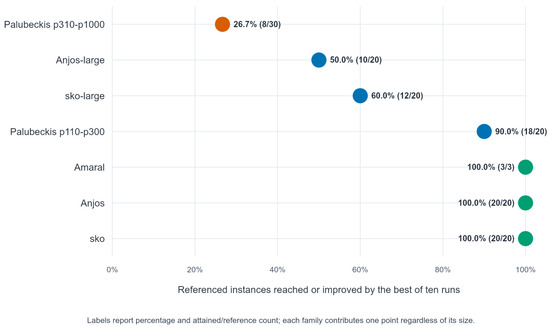
Table 3 separates best-of-ten target attainment from run-level reliability. Every comparable run in the Amaral, Anjos, and traditional Sko families matched its reference. The p110–p300 set also performed strongly: 18 of 20 instances reached the reference in at least one run and 146 of 200 runs matched it. The three more difficult large-scale groups retained small average gaps, but exact matches were less frequent.

Table 3. Results by benchmark family. “Best ≤ ref.” counts instances whose best of ten runs reached or improved the study reference. Mean gaps are unweighted across referenced instances. RSD is the median instance-level relative standard deviation.

Family	Files	Ref.	Best ≤ Ref.	Run Hits	Hit Rate	Mean Best Gap	Mean-Average Gap	Median RSD
Amaral	3	3	3	30/30	100.0%	0.000000%	0.000000%	0.000000%
Anjos	21	20	20	200/200	100.0%	0.000000%	0.000000%	0.000000%
Anjos-large	20	20	10	30/200	15.0%	0.001416%	0.007742%	0.003738%
Sko	23	20	20	200/200	100.0%	0.000000%	0.000000%	0.000000%
Sko-large	20	20	12	42/200	21.0%	0.000925%	0.005564%	0.003594%
p110–p300	20	20	18	146/200	73.0%	0.000041%	0.000916%	0.000046%
p310–p1000	30	30	8	17/300	5.67%	0.004507%	0.011356%	0.004310%
All	137	133	91	665/1330	50.0%	0.001375%	0.004700%	0.000551%

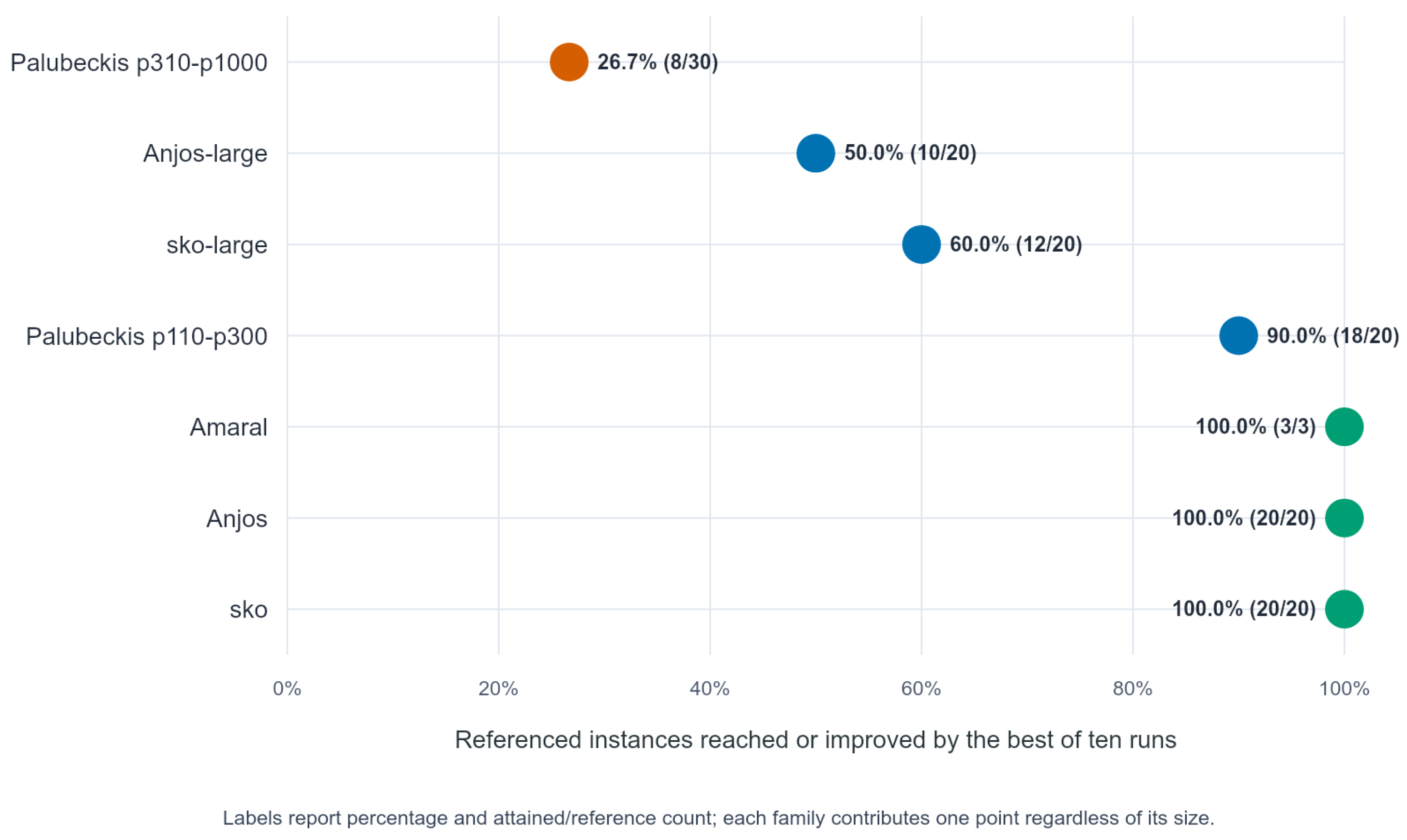
Figure 1 reports the best-of-ten attainment rate as one percentage point per benchmark family. The attained/reference counts remain printed beside every point, while the common 0–100% scale avoids giving visually greater weight to families merely because they contain more instances.

Figure 1. Best-of-ten reference attainment normalized within each benchmark family. Point positions encode percentages; labels give both percentages and attained/reference counts. Orange denotes 40% attainment, blue denotes 80–90% attainment, and green denotes 100% attainment.

5.2. Distribution of Gaps and Scaling Behavior

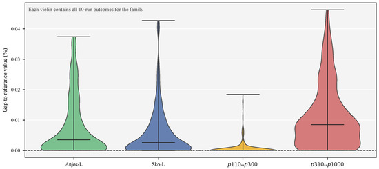
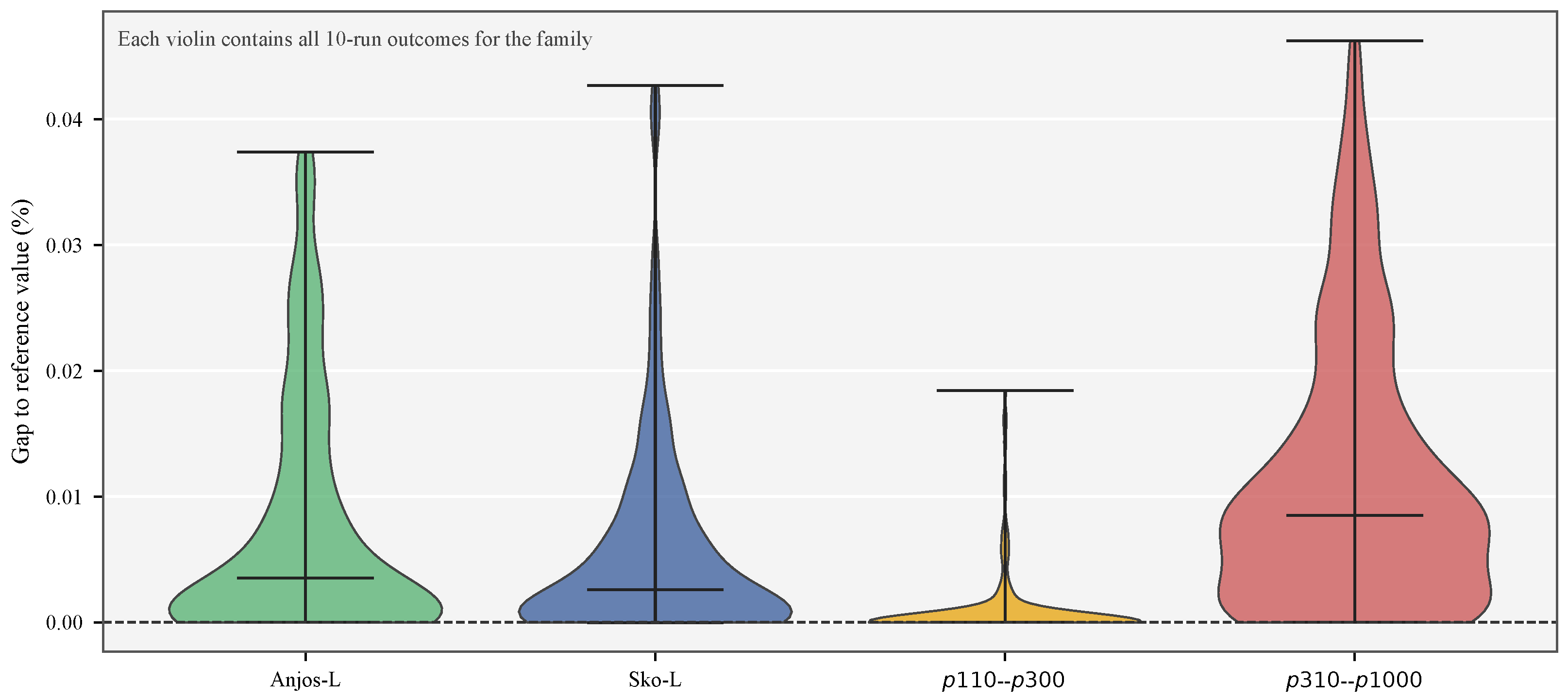
The violin plots in Figure 2 use all run-level outcomes in the four families where nonzero gaps occur regularly. The distributions are concentrated close to zero. The p110–p300 family is especially narrow, while p310–p1000 has the largest median and upper tail. The shapes also show why best-only reporting is insufficient: a family can reach its reference on selected seeds while still having a visibly positive distribution of ordinary-run gaps.

Figure 2. Run-level gap distributions for the four nontrivial benchmark families. Each violin pools the ten-run outcomes of every referenced instance in that family; horizontal internal bars mark the median and extrema. Negative values are possible when a run improves the reference snapshot.

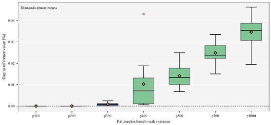
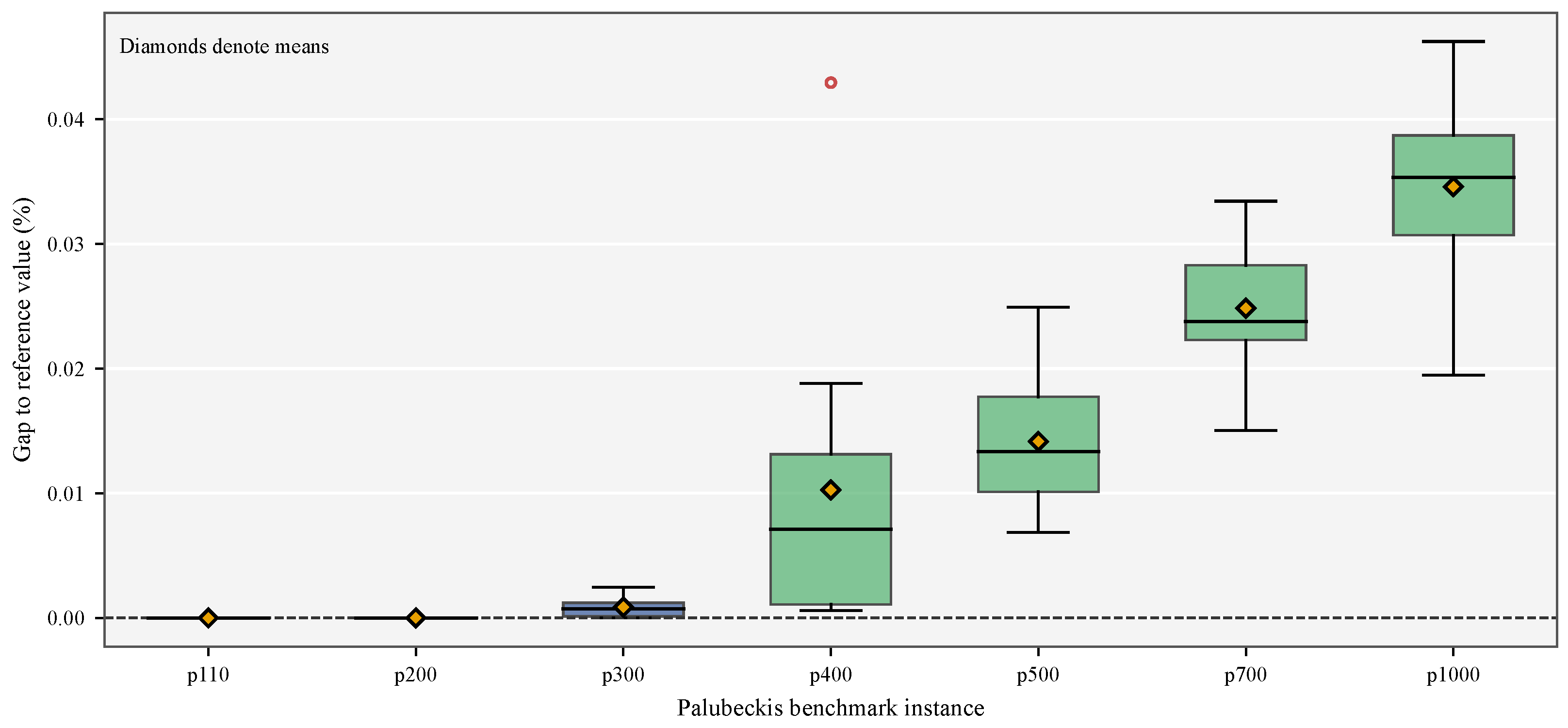
Figure 3 gives a complementary instance-level view for seven Palubeckis instances. The reference is matched by every run on p110 and p200. Dispersion becomes visible at p300 and grows gradually from p400 to p1000. Even at p1000, however, all ten outcomes remain within 0.05% of the reference.

Figure 3. Ten-run box plots of percentage gaps for representative Palubeckis instances. Diamonds denote means. Open circles denote observations beyond 1.5 times the interquartile range. Blue boxes denote p110–p300 instances, and green boxes denote p400–p1000 instances. The sequence illustrates the transition from deterministic reference matching on smaller cases to small but persistent positive gaps at larger scales.

Table 4 provides the objective values behind the selected distributions. The best and mean gaps remain small in absolute percentage terms, but the separation between them grows with n. At p1000, for example, the best gap is 0.019483% and the mean gap is 0.034592%. Such differences are small relative to the objective magnitude but meaningful when comparing mature SRFLP heuristics.

Table 4. Representative Palubeckis results. SD is the population standard deviation over ten runs and ${\overline{T}}_b$ is mean time to the best solution found in a run.

Inst.	Limit	Reference	Best	Mean	SD	Best Gap	Mean Gap	${\overline{\mathit{T}}}_{\mathit{b}}$ (s)
p110	60	4,435,868	4,435,868	4,435,868.0	0.0	0.000000%	0.000000%	1.04
p200	60	27,482,649.5	27,482,649.5	27,482,649.5	0.0	0.000000%	0.000000%	41.20
p300	120	95,937,735	95,937,735	95,938,573.2	770.8	0.000000%	0.000874%	102.82
p400	300	213,768,810.5	213,770,035.5	213,790,755.9	26,475.0	0.000573%	0.010266%	269.58
p500	300	465,570,835.5	465,602,770.5	465,636,714.9	23,956.2	0.006859%	0.014150%	292.50
p600	600	801,567,648.5	801,610,262.5	801,640,155.0	27,972.3	0.005316%	0.009046%	592.89
p700	600	1,158,462,254	1,158,636,466	1,158,750,034.0	58,919.5	0.015038%	0.024842%	592.85
p800	900	1,861,593,391	1,861,811,175	1,861,957,772.3	98,718.3	0.011699%	0.019574%	893.12
p900	900	2,600,003,561	2,600,590,090	2,600,797,437.2	136,753.0	0.022559%	0.030534%	893.44
p1000	900	3,426,646,969	3,427,314,593	3,427,832,326.9	242,442.1	0.019483%	0.034592%	895.09

5.3. Large-Instance Quality, Variability, and Time to Best

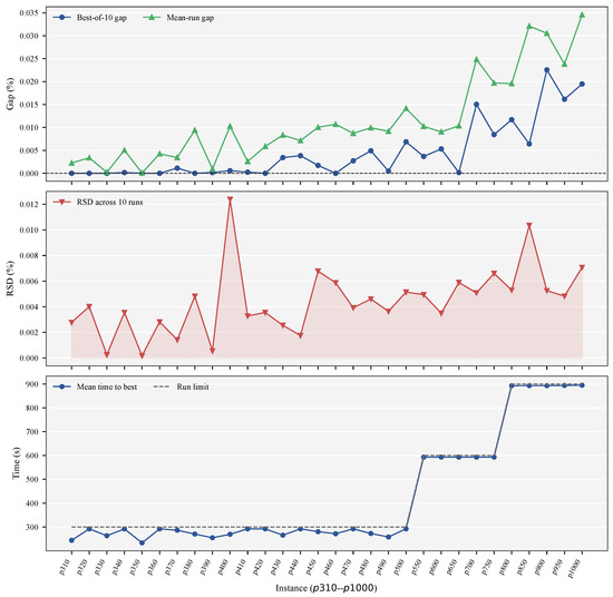
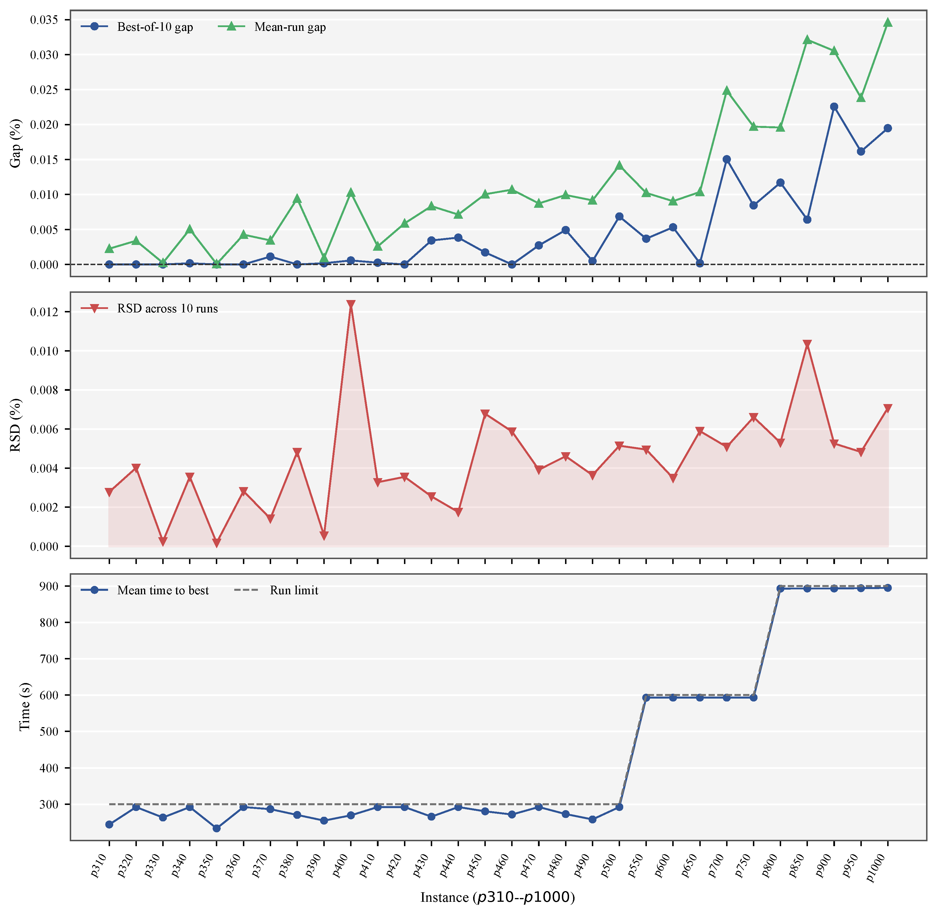
Figure 4 follows the three-indicator trend format of the KMPG study [11]. The upper panel shows best-of-ten and mean-run gaps for p310–p1000, the middle panel shows ten-run RSD, and the lower panel compares mean time to best with the run limit. Best-of-ten gaps are zero or nearly zero through much of the 310–650 range and generally increase thereafter, although difficulty is not monotone in n. The RSD stays below 0.013% for all 30 instances, demonstrating narrow seed-to-seed variation even when the reference is not reached.

Figure 4. Quality and timing trends on the 30 Palubeckis p310–p1000 instances: (top) best-of-ten and mean-run gaps; (middle) relative standard deviation over ten runs; and (bottom) mean time to best together with the run limit. The step changes in the lower panel are induced by the predetermined budget schedule.

The timing panel shows a different phenomenon. Mean time to best tracks the deadline closely for most large instances. Over the complete 1370-run corpus, the median normalized time to best is 0.870. In 631 runs (46.1%), the final improvement occurred during the last 10% of the budget. For p310–p1000, the family median is 0.975. The search therefore remains productive near the deadline; the nonzero large-instance gaps cannot be attributed simply to early stagnation followed by idle time.

5.4. Candidate Improvements Relative to the Reference Snapshot

Table 5 lists the two best-of-ten values that fall below the study reference snapshot. Both differences are small, integer-valued, and accompanied by feasible permutations in the run-level archive. For Sko-large 400_2, seven runs improve the reference, including five runs at 67,950,476 and two at 67,950,483. For Sko-large 500_2, the value 127,362,132 occurs once.

Table 5. Values below the 2023-era reference snapshot. These are candidate reference-table improvements, not claims of current best-known status.

Instance	Reference	Best	Difference	Runs Below Ref.	Best Seed
Sko-large 400_2	67,950,486	67,950,476	$-10$	7	20250301
Sko-large 500_2	127,362,138	127,362,132	$-6$	1	20250309

Both stored permutations were independently checked without calling the AMSA solver or its incremental-gain routines. One verifier summed every unordered flow-weighted center distance directly; a second used adjacent center gaps multiplied by the crossing flow. For 400_2 both formulas returned 67,950,476 and for 500_2 both returned 127,362,132, giving absolute and relative discrepancies of zero. The instance files, SHA-256 hashes, permutations, verifier, and reports are supplied. This establishes feasibility and objective correctness relative to the archived snapshot, but not current best-known status.

5.5. Seed Stability

Fifty-seven of the 137 instances returned exactly the same objective for all ten seeds. Across all instances, the median relative best-to-worst range was 0.001264%, and the maximum was 0.042680%. The median RSD was 0.000551%. Stability is strongest in the three traditional families, where every comparable run reaches the reference, and weakest—though still numerically tight—in the larger synthetic families. This pattern is consistent with a structure-informed first trajectory followed by random restarts: small and medium instances often converge to the same basin, while larger instances retain a modest stochastic spread.

5.6. Controlled Ablation and Conventional MSA Baseline

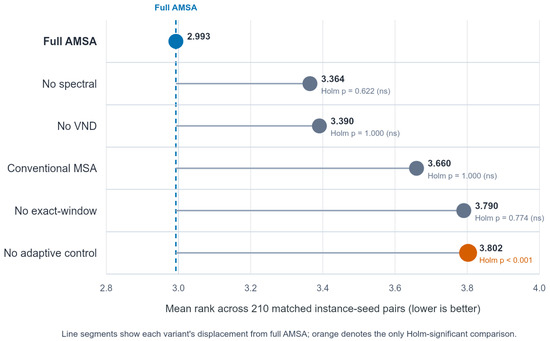
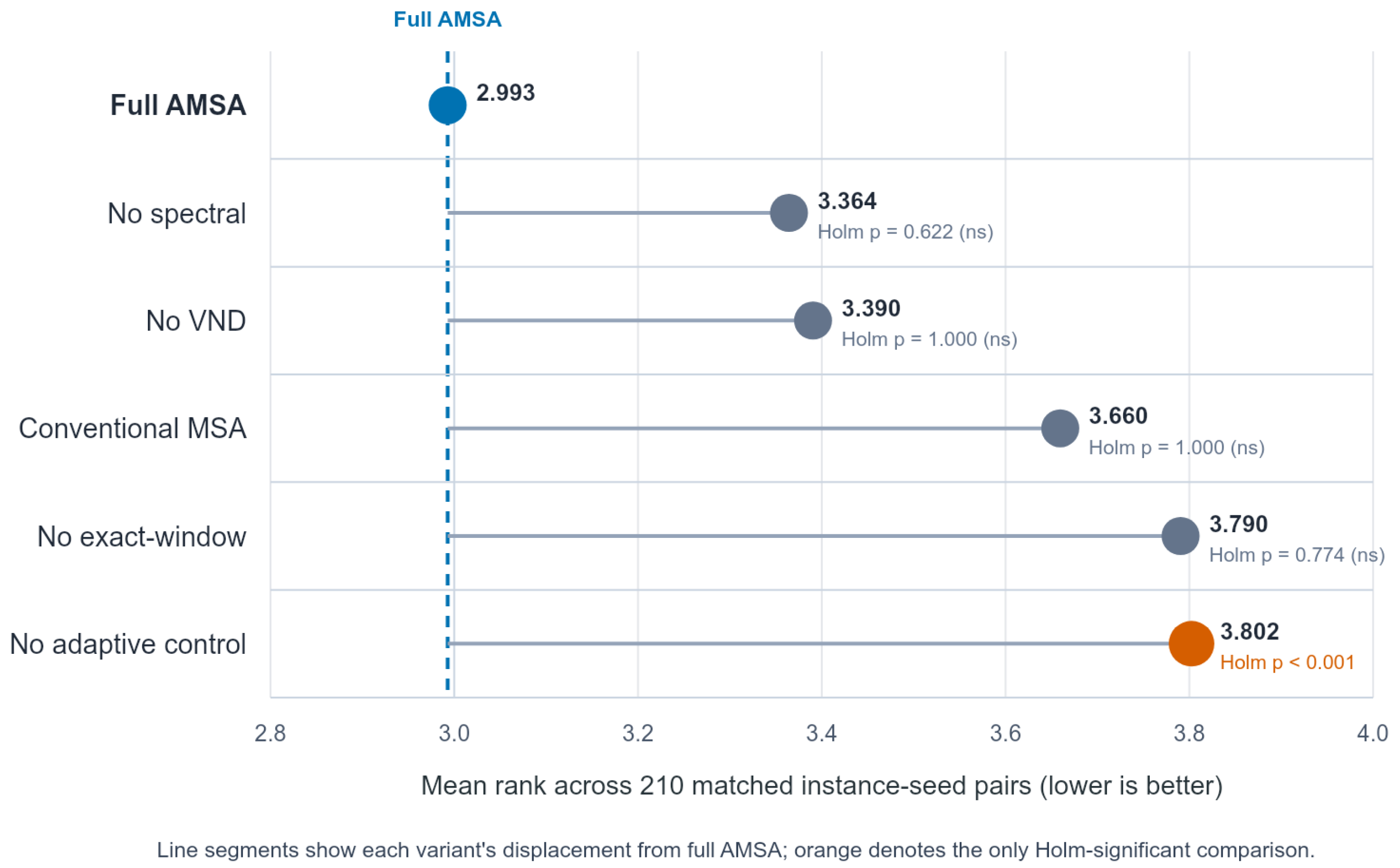
The six-variant experiment contains 210 matched instance–seed blocks per variant. Full AMSA had the smallest aggregate mean rank (2.993). Removing adaptive allocation gave the largest and clearest deterioration: full AMSA was better in 59.5% of pairs, no-adaptive was better in 3.3%, and 37.1% were ties; the paired Wilcoxon result remained significant after Holm correction ($p_{\mathrm{Holm}}=2.59\times {10}^{-15}$, effect $r=0.707$). The conventional MSA baseline and the no-spectral, no-VND, and no-exact-window variants did not differ significantly from full AMSA after correction. Consequently, the experiment supports the adaptive coordination mechanism but does not establish a statistically separable benefit for every individual module. Figure 5 visualizes the aggregate ranks, and Table 6 reports the paired comparisons.

Figure 5. Aggregate paired ranks for full AMSA, four component removals, and the conventional multi-start SA baseline. The figure summarizes ordering, whereas Table 6 provides the paired inference.

Table 6. Paired ablation results across 21 instances and ten seeds. Lower rank is better. Fractions compare each variant with full AMSA; Holm-adjusted p values cover the five comparisons.

Variant	Mean Rank	Full Better	Variant Better	Ties	${\mathit{p}}_{\mathbf{Holm}}$
Full AMSA	2.993	–	–	–	–
No spectral	3.364	30.0%	21.0%	49.0%	0.622
No VND	3.390	33.8%	28.6%	37.6%	1.000
Conventional MSA	3.660	41.0%	27.1%	31.9%	1.000
No exact-window	3.790	42.4%	25.2%	32.4%	0.774
No adaptive allocation	3.802	59.5%	3.3%	37.1%	$2.59\times {10}^{-15}$

5.7. Parameter Sensitivity

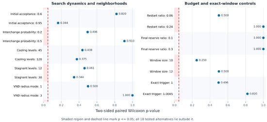
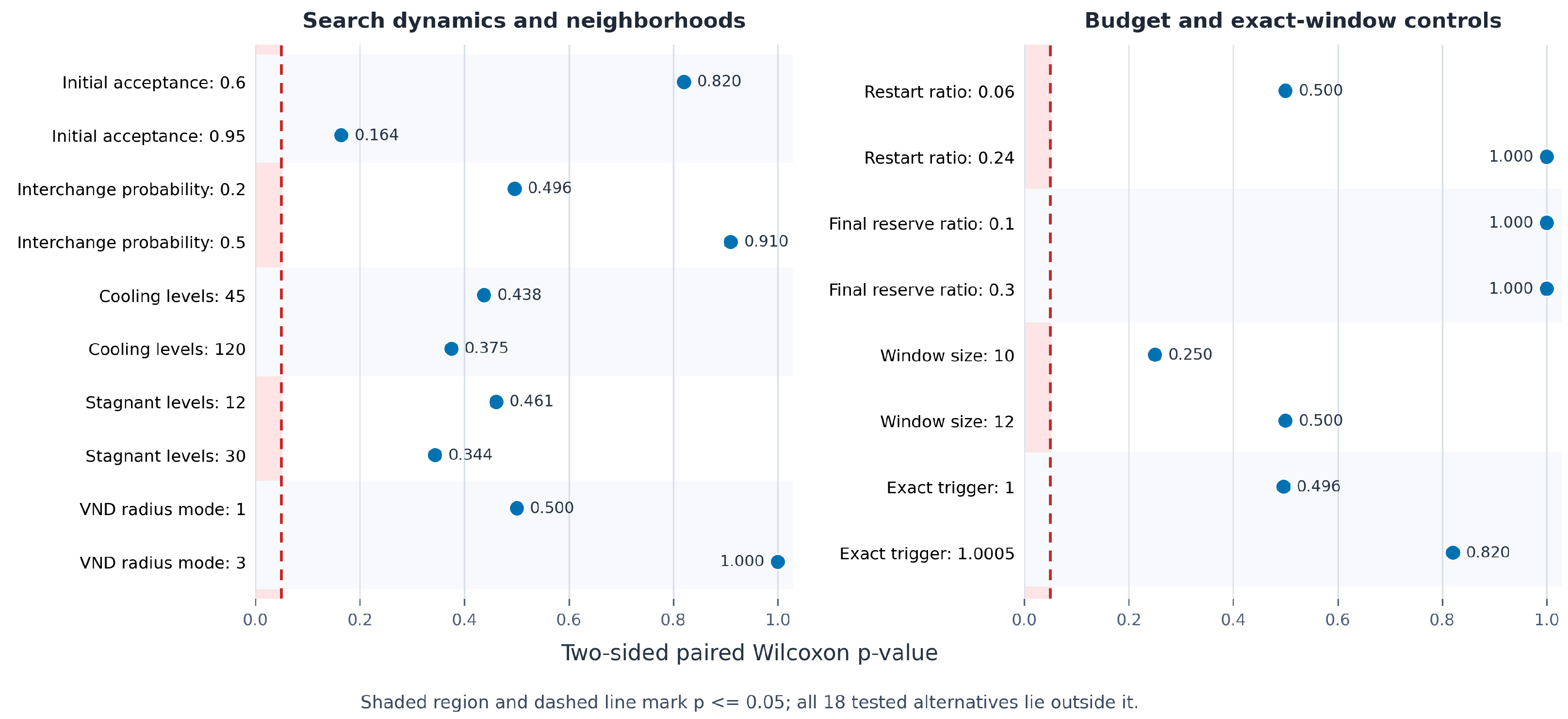
Nine control groups were varied one at a time over three levels: initial acceptance probability, interchange probability, cooling horizon, stagnation limit, VND radius mode, restart-budget ratio, final-reserve ratio, exact-window length, and exact-window trigger. Every level had 18 matched runs (six instances and three seeds). All 18 non-default levels gave two-sided paired Wilcoxon $p>0.05$ (range 0.164–1.000). The tested ranges therefore produced statistically indistinguishable objective values. We retain the pre-specified defaults as stable and reproducible operating points, not as theoretically or empirically proven optima. Figure 6 displays the paired p values for all non-default levels.

Figure 6. Paired Wilcoxon p values for every non-default sensitivity level versus its default, grouped into search-dynamics and budget/exact-window controls. The shaded region and dashed boundary mark $p\le 0.05$; all tested alternatives lie to the right.

5.8. Serial–Concurrent Execution Audit

Across 90 matched runs, serial execution required 30,600 s (8.50 h) of elapsed machine time, whereas concurrent execution required 8961 s (2.49 h), a 3.41-fold throughput improvement. The mean concurrent-minus-serial objective difference was $+198.51$ and was not significant (paired Wilcoxon $p=0.4328$). Mean time to best and solver time increased by only 0.0437 and 0.0060 s, respectively. Mean restarts decreased from 837.74 to 793.96 (5.23%), showing that CPU competition reduced the number of completed search trajectories within the same per-process wall-clock budget even though it did not significantly change objective quality in this subset. Table 7 summarizes these matched execution results.

Table 7. Serial and concurrent results for 90 matched runs on nine representative instances.

Metric	Serial	Concurrent	Concurrent − Serial
Elapsed machine time (h)	8.50	2.49	$-6.01$
Mean objective	936,999,116.43	936,999,314.94	$+198.51$
Mean time to best (s)	321.5399	321.5837	$+0.0437$
Mean solver time (s)	339.9867	339.9928	$+0.0060$
Mean restarts	837.74	793.96	$-43.79$

5.9. Exclusive Runtime Decomposition

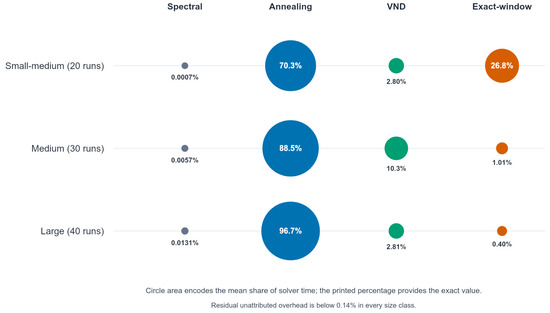
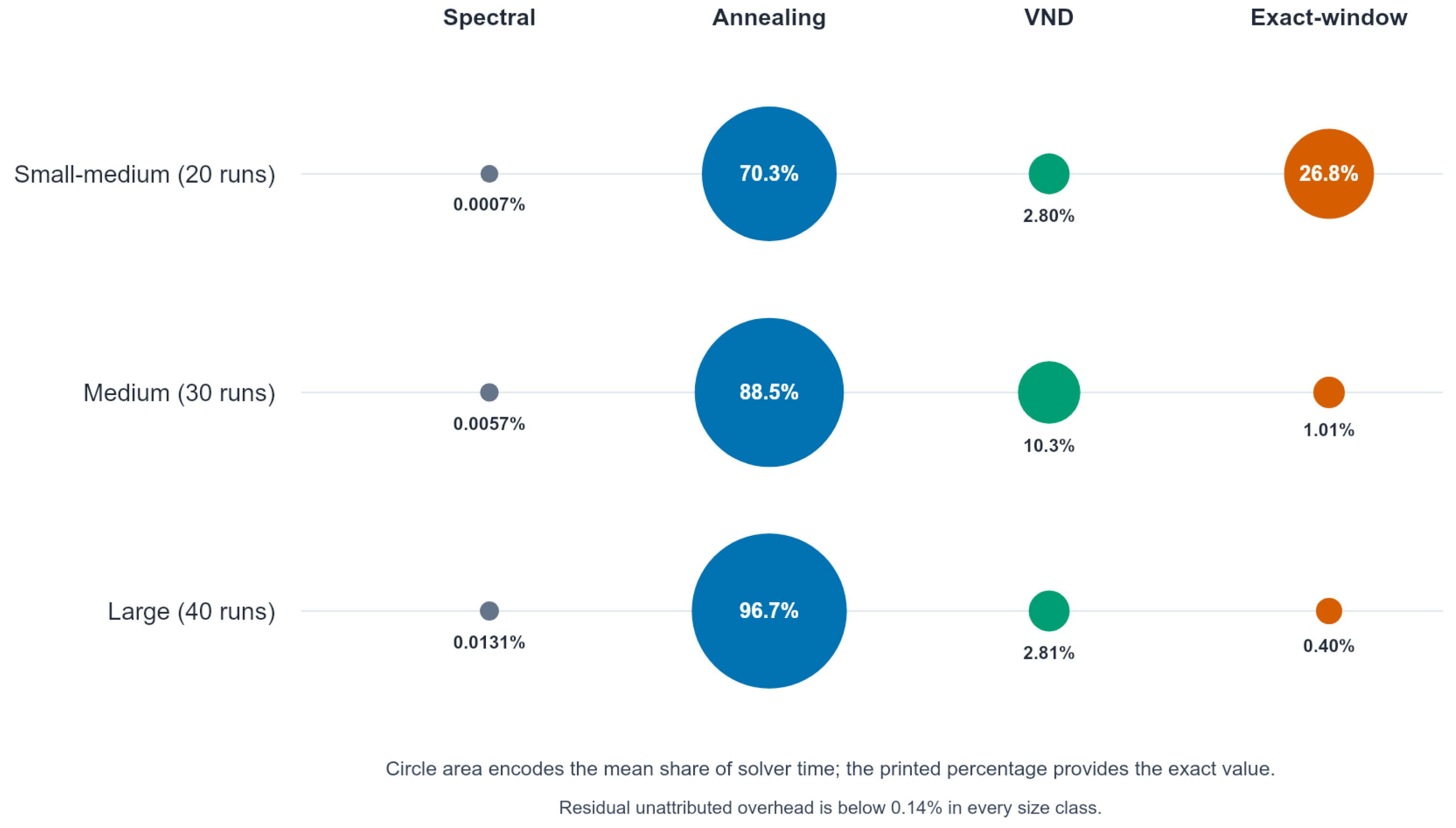
The timing experiment records exclusive stage totals rather than overlapping caller time. Annealing dominates increasingly with size: its mean share rises from 70.29% to 96.69%. Exact-window optimization accounts for 26.78% in the small–medium group but only 0.40% in the large group; VND accounts for 2.80–10.32%; spectral initialization remains below 0.014% in every size class. The unassigned share (deadline checks, bookkeeping, output, and other glue code) is below 0.14%. Thus, the exponential window module is visible chiefly on the smaller profiled cases, whereas large-instance runtime is overwhelmingly annealing. Table 8 reports the numerical shares, and Figure 7 visualizes their change across size classes.

Table 8. Mean exclusive runtime shares from 90 profiled runs.

Size Class	Runs	Spectral	Annealing	VND	Exact-Window
Small–medium	20	0.0007%	70.2858%	2.8023%	26.7810%
Medium	30	0.0057%	88.5238%	10.3223%	1.0137%
Large	40	0.0131%	96.6866%	2.8092%	0.3953%

Figure 7. Mean exclusive runtime shares by size class. Small residual differences to 100% are unattributed solver overhead.

6. Discussion

6.1. What the Computational Study Establishes

The computational study supports three principal conclusions. First, the implementation is reliable at the software and data-processing levels: all 1370 jobs completed, every reported layout was feasible, and independently regenerated summaries agreed with the archived results. Second, reference attainment is fully repeatable on the traditional Amaral, Anjos, and Sko sets and remains strong on p110–p300. Third, outcome distributions remain narrow on the large instances: the largest observed run-level reference gap is below 0.05%, and every family-level median RSD is below 0.005%.

The controlled results sharpen the causal boundary. Removing adaptive time allocation caused the only statistically clear deterioration after multiplicity correction, supporting the value of the deadline-aware coordination. Full AMSA nevertheless had the best aggregate rank. Differences for spectral initialization, VND, exact-window optimization, and the conventional baseline were not significant after Holm correction; their intended roles—structure-aware seeding, local intensification, coordinated fixed-exterior reorderings, and diversification—should therefore be read as design rationales rather than individually proven causes of improvement.

The existing production logs do not attribute every global-incumbent update to the stage that produced it. We therefore cannot give a defensible frequency with which exact-window calls strictly improved the incumbent without rerunning the instrumented search. Instead, we report its no-exact ablation and exclusive runtime share and preserve this missing counter as an explicit limitation. In particular, the nonsignificant no-exact comparison does not prove that the module is ineffective; it shows only that a separable quality effect was not detected under this design.

6.2. Interpretation of Reference Comparisons

Reference-target experiments are useful but easy to overstate. A zero gap means equality to the selected table, not necessarily a proven optimum. Conversely, a positive gap does not demonstrate that the algorithm is inferior to the method named as the reference source, because the original runs used different hardware, stopping rules, and often longer limits. The KMPG large-instance study used approximately one-hour cutoffs [11]; the present limits are at most 900 s. The newer OSA and matheuristic papers with exact-window optimization also use their own experimental platforms [12,13]. Accordingly, this paper reports target attainment and distributional quality, not a formal algorithm ranking.

The two candidate layouts illustrate a related distinction. Independent pairwise and cut-based recomputation has now verified both permutations and objective values exactly. However, verification of a candidate objective is different from verification of its rank in a changing best-known table. Because the latest public result repositories have not been exhaustively reconciled instance by instance, both values remain “verified improvements relative to the archived historical reference,” not claimed current upper bounds.

6.3. Time Allocation and Scalability

The timing data confirm that the deadline is active rather than nominal. Mean runtime utilization rises from approximately 80% for 10–30 s limits to more than 99% at 900 s, primarily because final intensification can end early on small instances, but large instances continue searching. Almost half of all runs improve in the final tenth of the budget. At p1000, the mean time to best is 895.09 s under a 900 s limit, and the p310–p1000 family median normalized time to best is 0.975. Late improvement is therefore common rather than an isolated p1000 anomaly. It also means that a 900 s cutoff does not demonstrate convergence; longer cutoffs could still improve these cases.

The exact-window optimization module has exponential dependence on the window length and is consequently capped at 14 facilities. Spectral initialization costs $O\left(I_s{n}^2\right)$ on dense data. The bounded VND radius controls cost for $n>250$ but may miss long-range restructuring. The profiling data show that large-instance cost is not dominated by spectral or exact-window processing: annealing consumes 96.69% of measured solver time in the large class. The declining best-of-ten attainment from 90.0% on p110–p300 to 26.7% on p310–p1000, including only 8 of 30 large p-instances reaching the historical reference, is therefore more plausibly associated with the restricted search trajectory and finite budget than with profiling overhead. Because time limits vary by size, conclusions are reported by family and size class rather than treating every run as an equal-budget contest. Potential extensions include adaptive window placement based on cut tension, occasional long-distance ejection chains, parallel restarts, and symmetry reduction.

6.4. Transferability

The coordination framework can transfer to another permutation problem when four ingredients are available: an interruptible stochastic trajectory, a valid incumbent at every interruption point, an incremental or otherwise fast neighborhood evaluator, and a bounded exact or strongly intensifying subproblem that can use a protected reserve. Examples may include sequencing or ordering problems with decomposable local windows. The SRFLP-specific cut identity, spectral flow graph, and fixed-exterior dynamic program would not transfer unchanged; each target problem would require its own move gains, structural seed, and exact subproblem. Transferability is therefore a research hypothesis, not established by the present SRFLP experiments.

7. Conclusions

This study presented a deadline-aware multi-start simulated annealing framework for the SRFLP. A 137-instance, ten-seed experiment produced 1370 successful runs; the best of ten reached or improved the historical study reference on 91 of 133 comparable instances, and the mean run-level relative gap was 0.004700%. Controlled evidence adds a six-variant ablation, a conventional MSA baseline, nine parameter groups, a serial–concurrent audit, exclusive stage profiling, and independent verification of two candidate layouts. Full AMSA obtained the best aggregate rank, while only removal of adaptive allocation differed significantly after Holm correction. The tested parameter ranges were statistically indistinguishable, and concurrent execution preserved objective quality in the representative audit while reducing restart throughput.

The evidence supports deadline-aware coordination, not a claim that every integrated module independently causes improvement. Reference attainment deteriorates on the largest p-instances, improvements often occur near the deadline, and recent literature comparisons remain unmatched in hardware and stopping budget. The two objective-verified candidate layouts improve only the archived snapshot until their current status is established. AMSA should therefore be viewed as a reproducible adaptive baseline and an experimental platform rather than as a demonstrated universal state-of-the-art method.

References

- Simmons, D.M. One-dimensional space allocation: An ordering algorithm. Oper. Res. 1969, 17, 812–826. [Google Scholar] [CrossRef] [Scilit]
- Love, R.F.; Wong, J.Y. On solving a one-dimensional space allocation problem with integer programming. INFOR Inf. Syst. Oper. Res. 1976, 14, 139–143. [Google Scholar] [CrossRef] [Scilit]
- Picard, J.C.; Queyranne, M. On the one-dimensional space allocation problem. Oper. Res. 1981, 29, 371–391. [Google Scholar] [CrossRef] [Scilit]
- Anjos, M.F.; Kennings, A.; Vannelli, A. A semidefinite optimization approach for the single-row layout problem with unequal dimensions. Discret. Optim. 2005, 2, 113–122. [Google Scholar] [CrossRef] [Scilit]
- Anjos, M.F.; Vannelli, A. Computing globally optimal solutions for single-row layout problems using semidefinite programming and cutting planes. INFORMS J. Comput. 2008, 20, 611–617. [Google Scholar] [CrossRef] [Scilit]
- Amaral, A.R.S.; Letchford, A.N. A polyhedral approach to the single row facility layout problem. Math. Program. 2013, 141, 453–477. [Google Scholar] [CrossRef] [Scilit]
- Kothari, R.; Ghosh, D. Insertion based Lin–Kernighan heuristic for single row facility layout. Comput. Oper. Res. 2013, 40, 129–136. [Google Scholar] [CrossRef] [Scilit]
- Kothari, R.; Ghosh, D. An efficient genetic algorithm for single row facility layout. Optim. Lett. 2014, 8, 679–690. [Google Scholar] [CrossRef] [Scilit]
- Cravo, G.L.; Amaral, A.R.S. A GRASP algorithm for solving large-scale single row facility layout problems. Comput. Oper. Res. 2019, 106, 49–61. [Google Scholar] [CrossRef] [Scilit]
- Palubeckis, G. Single row facility layout using multi-start simulated annealing. Comput. Ind. Eng. 2017, 103, 1–16. [Google Scholar] [CrossRef] [Scilit]
- Tang, L.; Li, Z.; Hao, J.K. Solving the single-row facility layout problem by K-medoids memetic permutation group. IEEE Trans. Evol. Comput. 2023, 27, 251–265. [Google Scholar] [CrossRef] [Scilit]
- Chen, B.; Lü, Z.; Su, Z.; Ding, J. An oscillation based simulated annealing algorithm for the single row facility layout problem. Eng. Appl. Artif. Intell. 2025, 159, 111551. [Google Scholar] [CrossRef] [Scilit]
- Pammer, T.; Sinnl, M. A matheuristic for solving the single row facility layout problem. Comput. Oper. Res. 2026, 189, 107397. [Google Scholar] [CrossRef] [Scilit]
- Amaral, A.R.S. A new lower bound for the single row facility layout problem. Discret. Appl. Math. 2009, 157, 183–190. [Google Scholar] [CrossRef] [Scilit]
- Anjos, M.F.; Yen, G. Provably near-optimal solutions for very large single-row facility layout problems. Optim. Methods Softw. 2009, 24, 805–817. [Google Scholar] [CrossRef] [Scilit]
- Hungerländer, P.; Rendl, F. A computational study and survey of methods for the single-row facility layout problem. Comput. Optim. Appl. 2013, 55, 1–20. [Google Scholar] [CrossRef] [Scilit]
- Keller, B.; Buscher, U. Single row layout models. Eur. J. Oper. Res. 2015, 245, 629–644. [Google Scholar] [CrossRef] [Scilit]
- Heragu, S.S.; Alfa, A.S. Experimental analysis of simulated annealing based algorithms for the layout problem. Eur. J. Oper. Res. 1992, 57, 190–202. [Google Scholar] [CrossRef] [Scilit]
- Samarghandi, H.; Eshghi, K. An efficient tabu algorithm for the single row facility layout problem. Eur. J. Oper. Res. 2010, 205, 98–105. [Google Scholar] [CrossRef] [Scilit]
- Datta, D.; Amaral, A.R.S.; Figueira, J.R. Single row facility layout problem using a permutation-based genetic algorithm. Eur. J. Oper. Res. 2011, 213, 388–394. [Google Scholar] [CrossRef] [Scilit]
- Guan, J.; Lin, G. Hybridizing variable neighborhood search with ant colony optimization for solving the single row facility layout problem. Eur. J. Oper. Res. 2016, 248, 899–909. [Google Scholar] [CrossRef] [Scilit]
- Wang, Z.; Xu, C. A thin-provisioned and functionalized memetic algorithm for the single row facility layout problem. Appl. Soft Comput. 2023, 146, 110716. [Google Scholar] [CrossRef] [Scilit]
- Martí, R.; Resende, M.G.C.; Ribeiro, C.C. Multi-start methods for combinatorial optimization. Eur. J. Oper. Res. 2013, 226, 1–8. [Google Scholar] [CrossRef] [Scilit]
- Fiedler, M. Algebraic connectivity of graphs. Czechoslov. Math. J. 1973, 23, 298–305. [Google Scholar] [CrossRef] [Scilit]
- Atkins, J.E.; Boman, E.G.; Hendrickson, B. A spectral algorithm for seriation and the consecutive ones problem. SIAM J. Comput. 1998, 28, 297–310. [Google Scholar] [CrossRef] [Scilit]
- Kirkpatrick, S.; Gelatt, C.D., Jr.; Vecchi, M.P. Optimization by simulated annealing. Science 1983, 220, 671–680. [Google Scholar] [CrossRef] [Scilit] [PubMed]
- Hajek, B. Cooling schedules for optimal annealing. Math. Oper. Res. 1988, 13, 311–329. [Google Scholar] [CrossRef] [Scilit]
- Mladenović, N.; Hansen, P. Variable neighborhood search. Comput. Oper. Res. 1997, 24, 1097–1100. [Google Scholar] [CrossRef] [Scilit]
- Held, M.; Karp, R.M. A dynamic programming approach to sequencing problems. J. Soc. Ind. Appl. Math. 1962, 10, 196–210. [Google Scholar] [CrossRef] [Scilit]
- Congram, R.K.; Potts, C.N.; van de Velde, S.L. An iterated dynasearch algorithm for the single-machine total weighted tardiness scheduling problem. INFORMS J. Comput. 2002, 14, 52–67. [Google Scholar] [CrossRef] [Scilit]
- Ergun, Ö.; Orlin, J.B. A dynamic programming methodology in very large scale neighborhood search applied to the traveling salesman problem. Discret. Optim. 2006, 3, 78–85. [Google Scholar] [CrossRef] [Scilit]
- McGeoch, C.C. Toward an experimental method for algorithm simulation. INFORMS J. Comput. 1996, 8, 1–15. [Google Scholar] [CrossRef] [Scilit]
- Kendall, G.; Bai, R.; Błażewicz, J.; De Causmaecker, P.; Gendreau, M.; John, R.; Li, J.; McCollum, B.; Pesch, E.; Qu, R.; et al. Good laboratory practice for optimization research. J. Oper. Res. Soc. 2016, 67, 676–689. [Google Scholar] [CrossRef] [Scilit]
- Birattari, M.; Dorigo, M. How to assess and report the performance of a stochastic algorithm on a benchmark problem: Mean or best result on a number of runs? Optim. Lett. 2007, 1, 309–311. [Google Scholar] [CrossRef] [Scilit]
Disclaimer/Publisher’s Note: The statements, opinions and data contained in all publications are solely those of the individual author(s) and contributor(s) and not of MDPI and/or the editor(s). MDPI and/or the editor(s) disclaim responsibility for any injury to people or property resulting from any ideas, methods, instructions or products referred to in the content. |
© 2026 by the authors. Licensee MDPI, Basel, Switzerland. This article is an open access article distributed under the terms and conditions of the Creative Commons Attribution (CC BY) license.