Stability and Local Bifurcations of a Discrete Predator–Prey System with Allee Effect and Holling-IV Functional Response

Abstract

This paper investigates the local dynamics of a discrete predator–prey system incorporating an Allee effect and a Holling-IV functional response. After nondimensionalization, a positivity-preserving discrete model is obtained by the semi-discretization method. The non-negative fixed points are classified and their local stability is established. The center manifold theorem and local bifurcation theory are then used to prove two transcritical bifurcations at the boundary fixed points $E_1$ and $E_2$ and a saddle-node bifurcation at the positive critical fixed point $E^{*}$. Numerical equilibrium branch diagrams and phase portraits illustrate these local results. The possible Neimark–Sacker bifurcation at $E_3$ and flip bifurcation at $E_4$ are beyond the present scope of this study.

1. Introduction and Preliminaries

Predator–prey models provide a basic framework for studying coexistence, extinction, stability, oscillations, and bifurcations [1,2]. Classical models often assume logistic prey growth, whereas a population at low density may exhibit reduced per capita growth or decline because of a strong Allee effect [2,3,4,5]. This mechanism may alter the number and stability of biologically meaningful equilibria and create threshold-dependent outcomes.

Holling type-I models may exhibit limit cycles, Hopf and cyclic-fold bifurcations, and bistability [3,6]; Holling type-II saturation may cause stability loss, Hopf bifurcations, and multiple limit cycles [1,7]; and Holling type-III responses can produce stability changes, Bogdanov–Takens, flip, and Neimark–Sacker bifurcations, and chaos [4,5,8,9]. Unlike these monotone responses, the simplified Holling-IV response is nonmonotone and represents inhibition at high prey density [10,11]. The closest studies differ from the present paper. References [12,13] investigate discrete predator–prey models with nonmonotone functional responses and derive stability and bifurcation results. Reference [11] also uses semi-discretization, but for a Leslie-type, ratio-dependent model with logistic prey growth, and analyzes one positive fixed point together with flip and Neimark–Sacker bifurcations. Reference [14] combines an Allee effect with Holling type-I predation and shows that changing the discretization can remove a reported flip bifurcation while yielding Neimark–Sacker and transcritical conditions. In contrast, the present map couples a strong Allee threshold with inhibitory Holling-IV predation, classifies zero, one, or two positive fixed points, and proves a saddle-node bifurcation at the collision of the two positive branches. Thus, the contribution lies in this interaction and the resulting equilibrium multiplicity, rather than in the standard boundary transcritical calculations alone.

Accordingly, the corresponding continuous predator–prey model takes the form [11]

$$\left\{\begin{array}{c}{\displaystyle \frac{dx}{dt}}=rx\left(1-{\displaystyle \frac{x}{K}}\right)(x-m)-{\displaystyle \frac{px}{x^2+a}}y,\hfill \\ {\displaystyle \frac{dy}{dt}}={\displaystyle \frac{epx}{x^2+a}}y-dy.\hfill \end{array}\right.$$

(1)

A strong Allee effect is characterized by a negative per capita growth rate below a positive population threshold and a positive rate immediately above it. In the absence of predators ($y=0$), the prey per capita growth rate is $G\left(x\right)=r(1-x/K)(x-m)$. Since $0<m<K$, $G\left(x\right)<0$ for $0<x<m$ and $G\left(x\right)>0$ for $m<x<K$. Thus, m is a positive strong Allee threshold. The variables and parameters are listed in Table 1.

Table 1. Biological meanings of variables and parameters in system (1).

Symbol	Biological Meaning
$x\left(t\right)$	Density of the prey population at time t
$y\left(t\right)$	Density of the predator population at time t
r	Growth coefficient of the prey (density-dependent)
K	Environmental carrying capacity of the prey
m	Allee threshold of the prey population
p	Scaling parameter of the predation rate
a	Inhibition parameter of the functional response
e	Conversion efficiency of the predator
d	Death rate of the predator

For the simplified Holling-IV functional response

$$H\left(x\right)={\displaystyle \frac{px}{x^2+a}},$$

direct differentiation gives

$$H^{\prime }\left(x\right)={\displaystyle \frac{p(a-x^2)}{{(x^2+a)}^2}}.$$

Hence, $H\left(x\right)$ increases for $0<x<\sqrt{a}$, decreases for $x>\sqrt{a}$, and attains its maximum

$$H\left(\sqrt{a}\right)={\displaystyle \frac{p}{2\sqrt{a}}}$$

at $x=\sqrt{a}$. Thus, p linearly scales the overall magnitude of the predation response without changing the location of its maximum, whereas a determines the prey-density level at which the response changes from increasing to decreasing and also influences the maximum response value. Since a is added to $x^2$, it has the dimensions of prey density squared and is not a conventional half-saturation constant. The decreasing response for $x>\sqrt{a}$ represents inhibition of predation at sufficiently high prey density, which is the ecological mechanism described by the simplified Holling-IV form.

For mathematical convenience, we first nondimensionalize system (1). Let

$$u={\displaystyle \frac{x}{K}},v={\displaystyle \frac{p}{r{K}^3}}y,\tau =rKt.$$

Furthermore, define the dimensionless parameters

$$\mu ={\displaystyle \frac{m}{K}},\alpha ={\displaystyle \frac{a}{K^2}},\beta ={\displaystyle \frac{ep}{r{K}^2}},\gamma ={\displaystyle \frac{d}{rK}}.$$

Since $0<m<K$, we have $0<\mu <1$.

Substituting these transformations into system (1), we derive the following nondimensional system:

$$\left\{\begin{array}{c}{\displaystyle \frac{du}{d\tau }}=u(1-u)(u-\mu )-{\displaystyle \frac{uv}{u^2+\alpha }},\hfill \\ {\displaystyle \frac{dv}{d\tau }}=v\left({\displaystyle \frac{\beta u}{u^2+\alpha }}-\gamma \right),\hfill \end{array}\right.$$

(2)

where

$$0<\mu <1,\alpha >0,\beta >0,\gamma >0.$$

In many ecological systems, population densities are observed at discrete time intervals. Moreover, discrete models may exhibit richer dynamics than their continuous counterparts, such as bifurcation, periodic oscillation, and chaos [9,12,13]. Therefore, it is natural to study the discrete version of system (2).

Now, we use a semi-discretization method to discretize system (2). Let $\left[\tau \right]$ denote the greatest integer not exceeding $\tau$. Consider the average rates of change of system (2) at integer times, namely, the following model [14]:

$$\left\{\begin{array}{c}{\displaystyle \frac{1}{u\left(\tau \right)}}{\displaystyle \frac{du}{d\tau }}=\left(1-u\left(\right[\tau \left]\right)\right)\left(u\left(\right[\tau \left]\right)-\mu \right)-{\displaystyle \frac{v\left(\right[\tau \left]\right)}{u^2\left(\left[\tau \right]\right)+\alpha }},\hfill \\ {\displaystyle \frac{1}{v\left(\tau \right)}}{\displaystyle \frac{dv}{d\tau }}={\displaystyle \frac{\beta u\left(\right[\tau \left]\right)}{u^2\left(\left[\tau \right]\right)+\alpha }}-\gamma .\hfill \end{array}\right.$$

(3)

One can see that a solution $\left(u\right(\tau ),v(\tau \left)\right)$ of system (3) for $\tau \in [0,+\infty )$ has the following properties:

• On the interval $[0,+\infty )$, $u\left(\tau \right)$ and $v\left(\tau \right)$ are continuous.
• ${\displaystyle \frac{du}{d\tau }}$ and ${\displaystyle \frac{dv}{d\tau }}$ exist everywhere when $\tau \in [0,+\infty )$, except possibly at the points $\{0,1,2,\dots \}$.
• System (3) holds on any interval $[n,n+1)$ with $n=0,1,2,\dots$.

The following system can be obtained by integrating system (3) over the interval $[n,\tau ]$ for any $\tau \in [n,n+1)$ and $n=0,1,2,\dots$:

$$\left\{\begin{array}{c}\ln {\displaystyle \frac{u\left(\tau \right)}{u\left(n\right)}}=\left[(1-u_n)(u_n-\mu )-{\displaystyle \frac{v_n}{u_n^2+\alpha }}\right](\tau -n),\hfill \\ \ln {\displaystyle \frac{v\left(\tau \right)}{v\left(n\right)}}=\left[{\displaystyle \frac{\beta u_n}{u_n^2+\alpha }}-\gamma \right](\tau -n).\hfill \end{array}\right.$$

(4)

where $u_n=u\left(n\right)$ and $v_n=v\left(n\right)$.

Exponentiating both equations in system (4), we obtain

$$\left\{\begin{array}{c}u\left(\tau \right)=u_n\exp \left\{\left[(1-u_n)(u_n-\mu )-{\displaystyle \frac{v_n}{u_n^2+\alpha }}\right](\tau -n)\right\},\hfill \\ v\left(\tau \right)=v_n\exp \left\{\left[{\displaystyle \frac{\beta u_n}{u_n^2+\alpha }}-\gamma \right](\tau -n)\right\}.\hfill \end{array}\right.$$

(5)

Letting $\tau \to {(n+1)}^{-}$ in system (5) produces

$$\left\{\begin{array}{c}{u}_{n+1}=u_n\exp \left[(1-u_n)(u_n-\mu )-{\displaystyle \frac{v_n}{u_n^2+\alpha }}\right],\hfill \\ v_{n+1}=v_n\exp \left[{\displaystyle \frac{\beta u_n}{u_n^2+\alpha }}-\gamma \right].\hfill \end{array}\right.$$

(6)

where

$$0<\mu <1,\alpha >0,\beta >0,\gamma >0.$$

and the parameters are the same as in system (2). System (6) will be considered in the sequel. It is easy to see that if $u_0>0$ and $v_0>0$, then $u_n>0$ and $v_n>0$ for all $n\ge 0$. Hence, the positive quadrant is positively invariant under system (6), which is consistent with the biological meaning of prey and predator populations.

Scope Limitation. The positivity argument above establishes only forward invariance of the positive quadrant; it does not prove boundedness, dissipativity, the existence of a compact absorbing region, uniform persistence, or a global basin structure. Accordingly, all stability and bifurcation conclusions below are local and do not imply global predator persistence or coexistence for arbitrary initial conditions. Section 2, Section 3, Section 4 and Section 5 present the fixed-point analysis, local bifurcations, numerical illustrations, and conclusions.

In the semi-discretization above, unit intervals $[n,n+1)$ are used in the dimensionless time $\tau$, so system (6) has the fixed step $h=1$. Since $\tau =rKt$, one iteration corresponds to ${\displaystyle \frac{1}{rK}}$ units of the original time. This is a modeling convention rather than a consequence forced by nondimensionalization. For a general $h>0$, both exponents in (6) would be multiplied by h. The fixed points and the critical values ${\beta }_0$, ${\beta }_1$, and ${\beta }_2$ remain unchanged, whereas the Jacobian multipliers and stability may depend on h. Therefore, all results in this paper concern $h=1$; a systematic analysis for general h is left for future work.

2. Existence and Stability of Fixed Points

2.1. Existence of Fixed Points

In this subsection, we discuss the existence of non-negative fixed points of the discrete system (6).

Let $E=(u,v)$ be a fixed point of system (6). Then, its coordinates satisfy

$$\left\{\begin{array}{c}u=u\exp \left[(1-u)(u-\mu )-{\displaystyle \frac{v}{u^2+\alpha }}\right],\hfill \\ v=v\exp \left[{\displaystyle \frac{\beta u}{u^2+\alpha }}-\gamma \right].\hfill \end{array}\right.$$

(7)

It is easy to see that system (6) always has the following three boundary fixed points:

$$E_0=(0,0),E_1=(1,0),E_2=(\mu ,0).$$

We now consider positive fixed points. Suppose that $u>0$ and $v>0$. Then, from (7), we have

$$(1-u)(u-\mu )-{\displaystyle \frac{v}{u^2+\alpha }}=0,$$

(8)

and

$${\displaystyle \frac{\beta u}{u^2+\alpha }}-\gamma =0.$$

(9)

By (8), we obtain

$$v=(u^2+\alpha )(1-u)(u-\mu ).$$

(10)

Since $v>0$, it follows directly from (10) that

$$\mu <u<1.$$

(11)

Equation (9) is equivalent to

$$\beta =\gamma {\displaystyle \frac{u^2+\alpha }{u}}=\gamma \left(u+{\displaystyle \frac{\alpha }{u}}\right).$$

(12)

Therefore, the existence of positive fixed points is equivalent to the existence of roots of

$$\varphi \left(u\right)=\gamma \left(u+{\displaystyle \frac{\alpha }{u}}\right)-\beta =0$$

(13)

in the interval $(\mu ,1)$.

For later use, define

$${\beta }_0:=2\gamma \sqrt{\alpha },{\beta }_1:=\gamma (1+\alpha ),{\beta }_2:=\gamma {\displaystyle \frac{{\mu }^2+\alpha }{\mu }}.$$

(14)

By direct calculation,

$${\varphi }^{\prime }\left(u\right)=\gamma \left(1-{\displaystyle \frac{\alpha }{u^2}}\right).$$

By the arithmetic-geometric mean inequality,

$${\beta }_1=\gamma (1+\alpha )\ge 2\gamma \sqrt{\alpha }={\beta }_0,{\beta }_2=\gamma \left(\mu +{\displaystyle \frac{\alpha }{\mu }}\right)\ge 2\gamma \sqrt{\alpha }={\beta }_0,$$

where equality holds if and only if $\alpha =1$ and $\alpha ={\mu }^2$, respectively. Moreover,

$${\beta }_1-{\beta }_2={\displaystyle \frac{\gamma (1-\mu )(\mu -\alpha )}{\mu }}.$$

Since $\gamma >0$ and $0<\mu <1$, it follows that ${\beta }_1>{\beta }_2$, ${\beta }_1={\beta }_2$, or ${\beta }_1<{\beta }_2$ according as $\alpha <\mu$, $\alpha =\mu$, or $\alpha >\mu$. Combining these comparisons gives all the orderings used in Table 2.

Table 2. Classification of positive fixed points.

Range of $\mathit{\alpha }$	Range of $\mathit{\beta }$	Number	Positive Fixed Point (s)
$0<\alpha \le {\mu }^2$	${\beta }_2<\beta <{\beta }_1$	1	$E_4=(u_2,v_2)$
${\mu }^2<\alpha <\mu$	$\beta ={\beta }_0$	1	$E^{*}=(\sqrt{\alpha },2\alpha (1-\sqrt{\alpha })(\sqrt{\alpha }-\mu ))$
	${\beta }_0<\beta <{\beta }_2$	2	$E_3=(u_1,v_1),E_4=(u_2,v_2)$
	${\beta }_2\le \beta <{\beta }_1$	1	$E_4=(u_2,v_2)$
$\alpha =\mu$	$\beta ={\beta }_0$	1	$E^{*}=(\sqrt{\alpha },2\alpha (1-\sqrt{\alpha })(\sqrt{\alpha }-\mu ))$
	${\beta }_0<\beta <{\beta }_1$	2	$E_3=(u_1,v_1),E_4=(u_2,v_2)$
$\mu <\alpha <1$	$\beta ={\beta }_0$	1	$E^{*}=(\sqrt{\alpha },2\alpha (1-\sqrt{\alpha })(\sqrt{\alpha }-\mu ))$
	${\beta }_0<\beta <{\beta }_1$	2	$E_3=(u_1,v_1),E_4=(u_2,v_2)$
	${\beta }_1\le \beta <{\beta }_2$	1	$E_3=(u_1,v_1)$
$\alpha \ge 1$	${\beta }_1<\beta <{\beta }_2$	1	$E_3=(u_1,v_1)$
In all other parameter regions, system (6) has no positive fixed point.

Finally, $\varphi \left(\mu \right)={\beta }_2-\beta$, $\varphi \left(1\right)={\beta }_1-\beta$, and, when $\mu <\sqrt{\alpha }<1$, $\varphi \left(\sqrt{\alpha }\right)={\beta }_0-\beta$. Since ${\varphi }^{\prime }$ changes sign only at $\sqrt{\alpha }$, $\varphi$ is increasing on $(\mu ,1)$ for $\alpha \le {\mu }^2$, decreasing there for $\alpha \ge 1$, and decreases and then increases for ${\mu }^2<\alpha <1$. Comparing these values with zero yields exactly the classification in Table 2.

Here, throughout the table,

$$u_1={\displaystyle \frac{\beta -\sqrt{{\beta }^2-4{\gamma }^2\alpha }}{2\gamma }},u_2={\displaystyle \frac{\beta +\sqrt{{\beta }^2-4{\gamma }^2\alpha }}{2\gamma }},$$

and

$$v_i=(u_i^2+\alpha )(1-u_i)(u_i-\mu ),i=1,2.$$

(15)

When two positive fixed points exist,

$$E_3=(u_1,v_1),E_4=(u_2,v_2),$$

and, in particular,

$$\mu <u_1<\sqrt{\alpha }<u_2<1.$$

2.2. Local Stability of Fixed Points

Before analyzing the local stability of fixed points, we first introduce the following definition and lemma.

Definition 1.

Let $E(x,y)$ be a fixed point of a two-dimensional discrete system with multipliers ${\lambda }_1$ and ${\lambda }_2$:

(i) 

If $|{\lambda }_1| <1$ and $|{\lambda }_2| <1$, then $E(x,y)$ is called a sink, and a sink is locally asymptotically stable.

(ii) 

If $|{\lambda }_1| >1$ and $|{\lambda }_2| >1$, then $E(x,y)$ is called a source, and a source is locally asymptotically unstable.

(iii) 

If $|{\lambda }_1| <1$ and $|{\lambda }_2| >1$, or $|{\lambda }_1| >1$ and $|{\lambda }_2| <1$, then $E(x,y)$ is called a saddle.

(iv) 

If either $|{\lambda }_1| =1$ or $|{\lambda }_2| =1$, then $E(x,y)$ is called non-hyperbolic.

Lemma 1.

Let

$$F\left(\lambda \right)={\lambda }^2+B\lambda +C,$$

where B and C are two real constants. Suppose that ${\lambda }_1$ and ${\lambda }_2$ are two roots of $F\left(\lambda \right)=0$. Then, the following statements hold:

(i) 

If $F\left(1\right)>0$, then

(i.1) 

$|{\lambda }_1| <1$ and $|{\lambda }_2| <1$ if and only if $F(-1)>0$ and $C<1$;

(i.2) 

${\lambda }_1=-1$ and ${\lambda }_2\ne -1$ if and only if $F(-1)=0$ and $B\ne 2$;

(i.3) 

$|{\lambda }_1| <1$ and $|{\lambda }_2| >1$ if and only if $F(-1)<0$;

(i.4) 

$|{\lambda }_1| >1$ and $|{\lambda }_2| >1$ if and only if $F(-1)>0$ and $C>1$;

(i.5) 

${\lambda }_1$ and ${\lambda }_2$ are a pair of conjugate complex roots and $|{\lambda }_1| = |{\lambda }_2| =1$ if and only if $-2<B<2$ and $C=1$;

(i.6) 

${\lambda }_1={\lambda }_2=-1$ if and only if $F(-1)=0$ and $B=2$.

(ii) 

If $F\left(1\right)=0$, namely, 1 is one root of $F\left(\lambda \right)=0$, then the other root λ satisfies $\left|\lambda \right|<(=,>)1$ according to $\left|C\right|<(=,>)1$.

(iii) 

If $F\left(1\right)<0$, then $F\left(\lambda \right)=0$ has one root lying in $(1,+\infty )$. Moreover, we have the following:

(iii.1) 

The other root λ satisfies $\lambda <-1$ if and only if $F(-1)<0$ and satisfies $\lambda =-1$ if and only if $F(-1)=0$;

(iii.2) 

The other root satisfies $-1<\lambda <1$ if and only if $F(-1)>0$.

A direct calculation for system (6) gives

$$J(u,v)=\left(\begin{array}{cc}\left[1+u(1+\mu -2u)+{\displaystyle \frac{2u^{2}v}{{(u^2+\alpha )}^2}}\right]e^{(1-u)(u-\mu )-{\displaystyle \frac{v}{u^2+\alpha }}}& -{\displaystyle \frac{u}{u^2+\alpha }}{e}^{(1-u)(u-\mu )-{\displaystyle \frac{v}{u^2+\alpha }}}\\ \beta v{\displaystyle \frac{\alpha -u^2}{{(u^2+\alpha )}^2}}{e}^{{\displaystyle \frac{\beta u}{u^2+\alpha }}-\gamma }& e^{{\displaystyle \frac{\beta u}{u^2+\alpha }}-\gamma }\end{array}\right).$$

2.2.1. Local Stability of Boundary Fixed Points

At $E_0=(0,0)$, the Jacobian matrix is

$$J\left(E_0\right)=\left(\begin{array}{cc}{e}^{-\mu }& 0\\ 0& e^{-\gamma }\end{array}\right).$$

Since $0<e^{-\mu }<1$ and $0<e^{-\gamma }<1$, $E_0$ is a sink and hence is locally asymptotically stable.

In what follows, we analyze the local stability of the two nonzero boundary fixed points

$$E_1=(1,0),E_2=(\mu ,0).$$

By applying Definition 1 to the eigenvalues of the Jacobian matrix, we obtain the following local stability results for the boundary fixed points $E_1=(1,0)$ and $E_2=(\mu ,0)$, respectively.

Theorem 1.

For the boundary fixed point $E_1=(1,0)$ of system (6), the following statements are true:

(1) 

If $0<\beta <{\beta }_1$, then $E_1$ is a sink;

(2) 

If $\beta ={\beta }_1$, then $E_1$ is non-hyperbolic;

(3) 

If $\beta >{\beta }_1$, then $E_1$ is a saddle.

Proof. 

At $E_1=(1,0)$, the Jacobian matrix is

$$J\left(E_1\right)=\left(\begin{array}{cc}\mu & -{\displaystyle \frac{1}{1+\alpha }}\\ 0& \exp \left({\displaystyle \frac{\beta }{1+\alpha }}-\gamma \right)\end{array}\right).$$

Since $J\left(E_1\right)$ is an upper triangular matrix, its eigenvalues are

$${\lambda }_1=\mu ,{\lambda }_2=\exp \left({\displaystyle \frac{\beta }{1+\alpha }}-\gamma \right).$$

Since $0<\mu <1$, $|{\lambda }_1|<1$. Hence the local stability of $E_1$ is determined by ${\lambda }_2$. Moreover, since ${\lambda }_2>0$, one has ${\lambda }_2<1$, ${\lambda }_2=1$, or ${\lambda }_2>1$ when $\beta <{\beta }_1$, $\beta ={\beta }_1$, or $\beta >{\beta }_1$, respectively. □

Remark 1.

Theorem 1 describes the ecological state where the prey population persists at its carrying capacity while the predator is absent, corresponding to $E_1=(1,0)$. When β is small, the energy gain from predation is insufficient to sustain predator growth, and a predator population introduced at sufficiently low density eventually dies out, leading the system to remain in a prey-only state. When β exceeds the critical value ${\beta }_1$, this state loses stability, indicating that predators are able to invade and alter the ecosystem structure.

Theorem 2.

The local stability of the boundary fixed point $E_2=(\mu ,0)$ of system (6) is classified as follows:

(1) 

If $0<\beta <{\beta }_2$, then $E_2$ is a saddle;

(2) 

If $\beta ={\beta }_2$, then $E_2$ is non-hyperbolic;

(3) 

If $\beta >{\beta }_2$, then $E_2$ is a source.

Proof. 

At $E_2=(\mu ,0)$, the Jacobian matrix is

$$J\left(E_2\right)=\left(\begin{array}{cc}1+\mu -{\mu }^2& -{\displaystyle \frac{\mu }{{\mu }^2+\alpha }}\\ 0& \exp \left({\displaystyle \frac{\beta \mu }{{\mu }^2+\alpha }}-\gamma \right)\end{array}\right).$$

Since $J\left(E_2\right)$ is an upper triangular matrix, its eigenvalues are

$${\lambda }_1=1+\mu -{\mu }^2,{\lambda }_2=\exp \left({\displaystyle \frac{\beta \mu }{{\mu }^2+\alpha }}-\gamma \right).$$

Since $0<\mu <1$, we have

$${\lambda }_1=1+\mu -{\mu }^2=1+\mu (1-\mu )>1.$$

Thus,

$$|{\lambda }_1| >1.$$

Since ${\lambda }_2>0$, we have ${\lambda }_2<1$, ${\lambda }_2=1$, or ${\lambda }_2>1$ when $\beta <{\beta }_2$, $\beta ={\beta }_2$, or $\beta >{\beta }_2$, respectively. □

From the above theorems, the boundary fixed point $E_1$ changes from a sink to a saddle as $\beta$ passes through the critical value ${\beta }_1$, while $E_2$ changes from a saddle to a source as $\beta$ passes through the critical value ${\beta }_2$. In both critical cases, the Jacobian matrix has an eigenvalue $\lambda =1$, which will be considered in the subsequent bifurcation analysis.

Remark 2.

Theorem 2 corresponds to the state $E_2=(\mu ,0)$, where the prey population is at the Allee threshold and the predator is absent. This state represents a critical low-density survival boundary for the prey population under the Allee effect. The result shows that this equilibrium is not robust to perturbations or predation pressure, and the system tends to move away from this threshold state, leading to alternative population dynamics.

2.2.2. Local Stability of Positive Fixed Points

In this subsubsection, we discuss the local stability of positive fixed points of system (6). Let $E=(u,v)$ be a positive fixed point of system (6). Then,

$$\mu <u<1,$$

and

$$v=(u^2+\alpha )(1-u)(u-\mu ),$$

$${\displaystyle \frac{\beta u}{u^2+\alpha }}=\gamma .$$

At a positive fixed point, the two exponential terms in the Jacobian matrix are equal to 1. Thus, the Jacobian matrix at $E=(u,v)$ becomes

$$J\left(E\right)=\left(\begin{array}{cc}1+u(1+\mu -2u)+{\displaystyle \frac{2u^2(1-u)(u-\mu )}{u^2+\alpha }}& -{\displaystyle \frac{u}{u^2+\alpha }}\\ {\displaystyle \frac{\beta v(\alpha -u^2)}{{(u^2+\alpha )}^2}}& 1\end{array}\right),$$

The characteristic equation of $J\left(E\right)$ can be written as

$$F\left(\lambda \right)={\lambda }^2+B\left(u\right)\lambda +C\left(u\right),$$

where

$$B\left(u\right)=-\left[2+u(1+\mu -2u)+{\displaystyle \frac{2u^2(1-u)(u-\mu )}{u^2+\alpha }}\right],$$

and

$$C\left(u\right)=1+u(1+\mu -2u)+{\displaystyle \frac{2u^2(1-u)(u-\mu )}{u^2+\alpha }}+\gamma {\displaystyle \frac{(1-u)(u-\mu )(\alpha -u^2)}{u^2+\alpha }}.$$

Therefore,

$$F\left(1\right)=\gamma {\displaystyle \frac{(1-u)(u-\mu )(\alpha -u^2)}{u^2+\alpha }},$$

and

$$F(-1)=4+2u(1+\mu -2u)+{\displaystyle \frac{4u^2(1-u)(u-\mu )}{u^2+\alpha }}+\gamma {\displaystyle \frac{(1-u)(u-\mu )(\alpha -u^2)}{u^2+\alpha }}.$$

Based on the characteristic equation obtained above and in Lemma 1, we now summarize the local stability of the positive fixed points.

For convenience, define

$$\begin{array}{cc}\hfill \delta & ={\displaystyle \frac{[4+2u_2(1+\mu -2u_2)](u_2^2+\alpha )+4u_2^2(1-u_2)(u_2-\mu )}{(1-u_2)(u_2-\mu )(u_2^2-\alpha )}},\hfill \\ \hfill {\Gamma }_{u_1}& =u_1(1+\mu -2u_1)+{\displaystyle \frac{2u_1^2(1-u_1)(u_1-\mu )}{u_1^2+\alpha }}+\gamma {\displaystyle \frac{(1-u_1)(u_1-\mu )(\alpha -u_1^2)}{u_1^2+\alpha }}.\hfill \end{array}$$

Here $\delta$ is an equilibrium-dependent threshold evaluated at $E_4=(u_2,v_2)$. Since $u_2$ depends on the model parameters through (15), conditions expressed in terms of $\delta$ are implicit. For notational simplicity, we retain $\delta$ below; ${\Gamma }_{u_1}$ is used for $E_3=(u_1,v_1)$.

Then, the local stability of positive fixed points can be classified as follows. For any positive fixed point $E=(u,v)$, we have $\mu <u<1$. Hence, from the expression of $F\left(1\right)$, the sign of $F\left(1\right)$ is determined by the sign of $\alpha -u^2$. Therefore, the stability of positive fixed points can be discussed according to the relative position of u and $\sqrt{\alpha }$.

First, consider the right-branch positive fixed point $E_4=(u_2,v_2)$. Since $u_2>\sqrt{\alpha }$, one has $F\left(1\right)<0$. By Lemma 1, $E_4$ has an eigenvalue greater than 1. Its remaining stability is determined by the sign of $F(-1)$. Solving $F(-1)=0$ gives the critical value $\delta$. Therefore, $E_4$ is a saddle if $0<\gamma <\delta$, non-hyperbolic if $\gamma =\delta$, and a source if $\gamma >\delta$.

Second, consider the critical positive fixed point $E^{*}$, where $u^{*}=\sqrt{\alpha }$. Here, $J\left(E^{*}\right)$ is upper triangular, and its two multipliers are

$${\lambda }_1=1,{\lambda }_2={\Lambda }_{*}=1+2\sqrt{\alpha }+2\mu \sqrt{\alpha }-\mu -3\alpha >0.$$

Hence, $E^{*}$ is non-hyperbolic.

Finally, for the left-branch positive fixed point $E_3=(u_1,v_1)$, $\mu <u_1<1$ and $u_1<\sqrt{\alpha }$; hence, $F\left(1\right)>0$. Moreover,

$$\begin{array}{cc}\hfill F(-1)=& 4(1-u_1^2)+2u_1(1+\mu )+{\displaystyle \frac{4u_1^2(1-u_1)(u_1-\mu )}{u_1^2+\alpha }}\hfill \\ & +\gamma {\displaystyle \frac{(1-u_1)(u_1-\mu )(\alpha -u_1^2)}{u_1^2+\alpha }}>0.\hfill \end{array}$$

Every term is positive since $\gamma >0$, $1-u_1>0$, $u_1-\mu >0$, and $\alpha -u_1^2>0$. Thus, by Lemma 1, $E_3$ is a sink, non-hyperbolic, or a source according as ${\Gamma }_{u_1}<0$, ${\Gamma }_{u_1}=0$, or ${\Gamma }_{u_1}>0$, respectively.

Combining the above three cases with the existence classification of positive fixed points in Section 2.1, we obtain the classifications summarized in Table 3, Table 4 and Table 5.

Table 3. Type of fixed point $E^{*}$.

Conditions		Eigenvalues	Properties
${\mu }^2<\alpha \le \mu$	$\beta ={\beta }_0$	$\left|{\lambda }_1\right|=1,\left|{\lambda }_2\right|>1$	non-hyperbolic
$\mu <\alpha <1$	$\beta ={\beta }_0$	$\left|{\lambda }_1\right|=1,\left|{\lambda }_2\right|>1\mathrm{or}\left|{\lambda }_2\right|<1$	non-hyperbolic

Table 4. Type of fixed point $E_3$.

Conditions			Eigenvalues	Properties
${\mu }^2<\alpha <\mu$	${\beta }_0<\beta <{\beta }_2$		$\left|{\lambda }_1\right|>1,\left|{\lambda }_2\right|>1$	source
$\alpha =\mu$	${\beta }_0<\beta <{\beta }_1$		$\left|{\lambda }_1\right|>1,\left|{\lambda }_2\right|>1$	source
$\mu <\alpha <1$	${\beta }_0<\beta <{\beta }_1$	${\Gamma }_{u_1}>0$	$\left|{\lambda }_1\right|>1,\left|{\lambda }_2\right|>1$	source
		${\Gamma }_{u_1}=0$	$\left|{\lambda }_1\right|=\left|{\lambda }_2\right|=1$	non-hyperbolic
		${\Gamma }_{u_1}<0$	$\left|{\lambda }_1\right|<1,\left|{\lambda }_2\right|<1$	sink
$\alpha \ge 1$	${\beta }_1<\beta <{\beta }_2$	${\Gamma }_{u_1}>0$	$\left|{\lambda }_1\right|>1,\left|{\lambda }_2\right|>1$	source
		${\Gamma }_{u_1}=0$	$\left|{\lambda }_1\right|=\left|{\lambda }_2\right|=1$	non-hyperbolic
		${\Gamma }_{u_1}<0$	$\left|{\lambda }_1\right|<1,\left|{\lambda }_2\right|<1$	sink

Table 5. Type of fixed point $E_4$.

Conditions			Eigenvalues	Properties
$0<\alpha \le {\mu }^2$	${\beta }_2<\beta <{\beta }_1$	$0<\gamma <\delta$	$\left|{\lambda }_1\right|>1,\left|{\lambda }_2\right|<1$	saddle
		$\gamma =\delta$	$\left|{\lambda }_1\right|>1,\left|{\lambda }_2\right|=1$	non-hyperbolic
		$\gamma >\delta$	$\left|{\lambda }_1\right|>1,\left|{\lambda }_2\right|>1$	source
${\mu }^2<\alpha <\mu$	${\beta }_0<\beta <{\beta }_1$	$0<\gamma <\delta$	$\left|{\lambda }_1\right|>1,\left|{\lambda }_2\right|<1$	saddle
		$\gamma =\delta$	$\left|{\lambda }_1\right|>1,\left|{\lambda }_2\right|=1$	non-hyperbolic
		$\gamma >\delta$	$\left|{\lambda }_1\right|>1,\left|{\lambda }_2\right|>1$	source
$\alpha =\mu$	${\beta }_0<\beta <{\beta }_1$	$0<\gamma <\delta$	$\left|{\lambda }_1\right|>1,\left|{\lambda }_2\right|<1$	saddle
		$\gamma =\delta$	$\left|{\lambda }_1\right|>1,\left|{\lambda }_2\right|=1$	non-hyperbolic
		$\gamma >\delta$	$\left|{\lambda }_1\right|>1,\left|{\lambda }_2\right|>1$	source
$\mu <\alpha <1$	${\beta }_0<\beta <{\beta }_1$	$0<\gamma <\delta$	$\left|{\lambda }_1\right|>1,\left|{\lambda }_2\right|<1$	saddle
		$\gamma =\delta$	$\left|{\lambda }_1\right|>1,\left|{\lambda }_2\right|=1$	non-hyperbolic
		$\gamma >\delta$	$\left|{\lambda }_1\right|>1,\left|{\lambda }_2\right|>1$	source

3. Bifurcation Analysis

In this section, we employ the center manifold theorem and local bifurcation theory to establish the transcritical bifurcations at $E_1$ and $E_2$ and the saddle-node bifurcation at $E^{*}$. The potential Neimark–Sacker case at $E_3$ and flip case at $E_4$ can be studied within the same center-manifold and normal-form framework. However, their distinct higher-order transversality, nonresonance, and nondegeneracy calculations are substantially more involved; they are therefore omitted here and left for future work [15,16,17,18].

3.1. Main Results

From Theorem 1, $E_1=(1,0)$ is non-hyperbolic when $\beta ={\beta }_1$. Thus, a local bifurcation may occur near $E_1$ as $\beta$ passes through the critical value ${\beta }_1$. The following result is obtained.

Theorem 3.

Assume that $\alpha \ne 1$. If β varies in a small neighborhood of ${\beta }_1$, then system (6) undergoes a transcritical bifurcation at $E_1=(1,0)$. Moreover, if $\alpha >1$, the positive branch $E_3$ exists for $\beta >{\beta }_1$ and is locally asymptotically stable; if $0<\alpha <1$, the positive branch $E_4$ exists for $\beta <{\beta }_1$ and is a saddle.

Remark 3.

Theorem 3 is a local result. Only when $\alpha >1$ may nearby solutions approach the locally stable coexistence equilibrium. When $0<\alpha <1$, crossing ${\beta }_1$ does not imply successful predator establishment or stable coexistence.

From Theorem 2, $E_2=(\mu ,0)$ is non-hyperbolic when $\beta ={\beta }_2$. Similarly, a local bifurcation may occur near $E_2$ as $\beta$ passes through the critical value ${\beta }_2$. We have the following result.

Theorem 4.

Assume that $\alpha \ne {\mu }^2$. System (6) undergoes a transcritical bifurcation at $E_2=(\mu ,0)$ as β crosses ${\beta }_2$. Moreover, if $0<\alpha <{\mu }^2$, the positive branch $E_4$ exists for $\beta >{\beta }_2$ and is a saddle; if $\alpha >{\mu }^2$, the positive branch $E_3$ exists for $\beta <{\beta }_2$ and is a source.

Remark 4.

This result is also local. The point $E_2$ is a predator-free state with the prey exactly at the Allee threshold, not a prey-extinction state. Since the nearby positive branch is unstable in both cases, this bifurcation alone does not demonstrate predator persistence or stable coexistence.

Remark 5.

The excluded cases $\alpha =1$ in Theorem 3 and $\alpha ={\mu }^2$ in Theorem 4 are degenerate because the quadratic coefficient of the corresponding reduced map vanishes. Hence, the standard transcritical nondegeneracy condition fails, and higher-order terms or a higher-codimension unfolding must be considered. These cases are not investigated here.

At the critical value $\beta ={\beta }_0$, the two positive fixed points coalesce at $E^{*}$. Hence, $E^{*}$ is non-hyperbolic, and a local bifurcation may occur as $\beta$ passes through ${\beta }_0$. We have the following result.

Theorem 5.

Assume that ${\mu }^2<\alpha <1$ and

$$\alpha \ne {\left({\displaystyle \frac{1+\mu +\sqrt{{\mu }^2-\mu +1}}{3}}\right)}^2.$$

If the parameter β varies in a small neighborhood of ${\beta }_0$, then system (6) undergoes a saddle-node bifurcation at

$$E^{*}=\left(\sqrt{\alpha },2\alpha (1-\sqrt{\alpha })(\sqrt{\alpha }-\mu )\right).$$

Remark 6.

Theorem 5 shows that the two positive fixed points are created or annihilated when β crosses ${\beta }_0$. Thus, the saddle-node bifurcation produces an abrupt change in the number of locally available coexistence equilibria.

3.2. Proofs of the Main Results

Proof of Theorem 3.

From the stability analysis of boundary fixed points, the eigenvalues of the Jacobian matrix of system (6) at $E_1=(1,0)$ are

$${\lambda }_1=\mu ,{\lambda }_2=\exp \left({\displaystyle \frac{\beta }{1+\alpha }}-\gamma \right).$$

Since $0<\mu <1$, one has

$$|{\lambda }_1| <1.$$

When $\beta ={\beta }_1$, we have ${\lambda }_2=1$. Thus, $E_1$ is a non-hyperbolic fixed point and a bifurcation may occur at $E_1$.

To study the bifurcation at $E_1$, let $x_n=u_n-1$ and $y_n=v_n$, and introduce a small perturbation parameter ${\eta }_n^{*}=\beta -{\beta }_1$ with $0< |{\eta }_n^{*}| \ll 1$. Then, $u_n=1+x_n$, $v_n=y_n$, and $\beta ={\beta }_1+{\eta }_n^{*}$. Furthermore, let ${\eta }_{n+1}^{*}={\eta }_n^{*}$. Then, system (6) can be transformed into the following extended system:

$$\left\{\begin{array}{c}{x}_{n+1}=(1+x_n)\exp \left[-x_n(1-\mu +x_n)-{\displaystyle \frac{y_n}{1+\alpha +2x_n+x_n^2}}\right]-1,\hfill \\ y_{n+1}=y_n\exp \left[\left({\beta }_1+{\eta }_n^{*}\right){\displaystyle \frac{1+x_n}{1+\alpha +2x_n+x_n^2}}-\gamma \right],\hfill \\ {\eta }_{n+1}^{*}={\eta }_n^{*}.\hfill \end{array}\right.$$

(16)

Taking the Taylor expansion of system (16) at $(x_n,y_n,{\eta }_n^{*})=(0,0,0)$, we obtain

$$\left\{\begin{array}{c}\begin{array}{cc}\hfill x_{n+1}=& a_{100}{x}_n+a_{010}{y}_n+a_{200}{x}_n^2+a_{110}{x}_n{y}_n+a_{020}{y}_n^2+o\left({\rho }_1^2\right),\hfill \\ \hfill y_{n+1}=& b_{010}{y}_n+b_{110}{x}_n{y}_n+b_{011}{y}_n{\eta }_n^{*}+o\left({\rho }_1^2\right),\hfill \\ \hfill {\eta }_{n+1}^{*}=& {\eta }_n^{*},\hfill \end{array}\hfill \end{array}\right.$$

(17)

where ${\rho }_1=\sqrt{x_n^2+y_n^2+{\left({\eta }_n^{*}\right)}^2}$, and the coefficients are given by

$$\begin{array}{cccccc}\hfill a_{100}& =\mu ,\hfill & \hfill a_{010}& =-{\displaystyle \frac{1}{1+\alpha }},\hfill & \hfill a_{200}& ={\displaystyle \frac{{\mu }^2-3}{2}},\hfill \\ \hfill a_{110}& ={\displaystyle \frac{2}{{(1+\alpha )}^2}}-{\displaystyle \frac{\mu }{1+\alpha }},\hfill & \hfill a_{020}& ={\displaystyle \frac{1}{2{(1+\alpha )}^2}},\hfill & \hfill b_{010}& =1,\hfill \\ \hfill b_{110}& ={\displaystyle \frac{\gamma (\alpha -1)}{1+\alpha }},\hfill & \hfill b_{011}& ={\displaystyle \frac{1}{1+\alpha }}.\hfill & & \end{array}$$

The linear part of system (17) is

$$\left(\begin{array}{c}{x}_{n+1}\\ y_{n+1}\\ {\eta }_{n+1}^{*}\end{array}\right)=\left(\begin{array}{ccc}\mu & -{\displaystyle \frac{1}{1+\alpha }}& 0\\ 0& 1& 0\\ 0& 0& 1\end{array}\right)\left(\begin{array}{c}{x}_n\\ y_n\\ {\eta }_n^{*}\end{array}\right).$$

The eigenvalues of the above matrix are

$${\lambda }_1=\mu ,{\lambda }_2=1,{\lambda }_3=1.$$

The corresponding eigenvectors can be chosen as

$${(1,0,0)}^T,{\left({\displaystyle \frac{1}{(1+\alpha )(\mu -1)}},1,0\right)}^T,{(0,0,1)}^T.$$

Thus, we take the transformation matrix

$$P=\left(\begin{array}{ccc}1& {\displaystyle \frac{1}{(1+\alpha )(\mu -1)}}& 0\\ 0& 1& 0\\ 0& 0& 1\end{array}\right).$$

Let

$$\left(\begin{array}{c}{x}_n\\ y_n\\ {\eta }_n^{*}\end{array}\right)=P\left(\begin{array}{c}{X}_n\\ Y_n\\ {\eta }_n\end{array}\right).$$

That is,

$$x_n=X_n+{\displaystyle \frac{1}{(1+\alpha )(\mu -1)}}{Y}_n,y_n=Y_n,{\eta }_n^{*}={\eta }_n.$$

Under this transformation, system (17) becomes

$$\left\{\begin{array}{c}\begin{array}{cc}\hfill X_{n+1}=& A_{100}{X}_n+A_{200}{X}_n^2+A_{110}{X}_n{Y}_n+A_{020}{Y}_n^2+A_{011}{Y}_n{\eta }_n+o\left({\tilde{\rho }}_2^2\right),\hfill \\ \hfill Y_{n+1}=& B_{010}{Y}_n+B_{110}{X}_n{Y}_n+B_{020}{Y}_n^2+B_{011}{Y}_n{\eta }_n+o\left({\tilde{\rho }}_2^2\right),\hfill \\ \hfill {\eta }_{n+1}=& {\eta }_n,\hfill \end{array}\hfill \end{array}\right.$$

(18)

where ${\tilde{\rho }}_2=\sqrt{X_n^2+Y_n^2+{\eta }_n^2}$, and the coefficients are

$$\begin{array}{cccccc}\hfill A_{100}& =\mu ,\hfill & \hfill A_{200}& ={\displaystyle \frac{{\mu }^2-3}{2}},\hfill & \hfill A_{110}& ={\displaystyle \frac{5+3\alpha -3\mu -\alpha \mu +\gamma (\alpha -1)}{{(1+\alpha )}^2(1-\mu )}},\hfill \\ \hfill A_{020}& =-{\displaystyle \frac{\alpha \gamma +\alpha -\gamma -2\mu +3}{{(1+\alpha )}^3{(1-\mu )}^2}},\hfill & \hfill A_{011}& ={\displaystyle \frac{1}{{(1+\alpha )}^2(1-\mu )}},\hfill & \hfill B_{010}& =1,\hfill \\ \hfill B_{110}& ={\displaystyle \frac{\gamma (\alpha -1)}{1+\alpha }},\hfill & \hfill B_{020}& ={\displaystyle \frac{\gamma (1-\alpha )}{{(1+\alpha )}^2(1-\mu )}},\hfill & \hfill B_{011}& ={\displaystyle \frac{1}{1+\alpha }}.\hfill \end{array}$$

Now, we consider the center manifold. Let

$$X=h(Y,\eta ),$$

where

$$h(0,0)=0,Dh(0,0)=0.$$

Assume that

$$h(Y,\eta )=c_{20}{Y}^2+c_{11}Y\eta +c_{02}{\eta }^2+o\left({\rho }_2^2\right),$$

where ${\rho }_2=\sqrt{Y^2+{\eta }^2}$. Using the center manifold invariance equation

$$h(Y_{n+1},{\eta }_{n+1})=X_{n+1},$$

and comparing the coefficients of the second-order terms, we obtain

$$c_{20}=-{\displaystyle \frac{\alpha \gamma +\alpha -\gamma -2\mu +3}{{(1+\alpha )}^3{(1-\mu )}^3}},c_{11}={\displaystyle \frac{1}{{(1+\alpha )}^2{(1-\mu )}^2}},c_{02}=0.$$

Therefore, the center manifold is given by

$$X=h(Y,\eta )=-{\displaystyle \frac{\alpha \gamma +\alpha -\gamma -2\mu +3}{{(1+\alpha )}^3{(1-\mu )}^3}}{Y}^2+{\displaystyle \frac{1}{{(1+\alpha )}^2{(1-\mu )}^2}}Y\eta +o\left({\rho }_2^2\right).$$

(19)

Restricting system (18) to the center manifold, we obtain the following reduced equation:

$$Y_{n+1}=g(Y_n,{\eta }_n),$$

where

$$g(Y,\eta )=Y+{\displaystyle \frac{1}{1+\alpha }}Y\eta +{\displaystyle \frac{\gamma (1-\alpha )}{{(1+\alpha )}^2(1-\mu )}}{Y}^2+o\left({\rho }_2^2\right).$$

(20)

From (20), we have

$$g(0,0)=0,g_Y(0,0)=1,g_{\eta }(0,0)=0,g_{Y\eta }(0,0)={\displaystyle \frac{1}{1+\alpha }}\ne 0.$$

Moreover,

$$g_{YY}(0,0)={\displaystyle \frac{2\gamma (1-\alpha )}{{(1+\alpha )}^2(1-\mu )}}.$$

Since

$$\gamma >0,0<\mu <1,$$

we have

$$g_{YY}(0,0)\ne 0$$

if and only if

$$\alpha \ne 1.$$

Therefore, if $\alpha \ne 1$, then all the conditions for a transcritical bifurcation are satisfied. Hence, system (6) undergoes a transcritical bifurcation at $E_1=(1,0)$ when $\beta ={\beta }_1$. This proves Theorem 3. □

Proof of Theorem 4.

By the stability analysis of boundary fixed points, the eigenvalues of the Jacobian matrix of system (6) at $E_2=(\mu ,0)$ are

$${\lambda }_1=1+\mu -{\mu }^2,{\lambda }_2=\exp \left({\displaystyle \frac{\beta \mu }{{\mu }^2+\alpha }}-\gamma \right).$$

Because $0<\mu <1$, we have

$${\lambda }_1=1+\mu -{\mu }^2=1+\mu (1-\mu )>1.$$

At $\beta ={\beta }_2$, we have ${\lambda }_2=1$. Consequently, $E_2$ is a non-hyperbolic fixed point and a bifurcation may occur at $E_2$.

For the bifurcation analysis at $E_2$, let $x_n=u_n-\mu$ and $y_n=v_n$ and introduce a small perturbation parameter ${\eta }_n^{*}=\beta -{\beta }_2$ with $0< |{\eta }_n^{*}| \ll 1$. Thus, $u_n=\mu +x_n$, $v_n=y_n$, and $\beta ={\beta }_2+{\eta }_n^{*}$. In addition, let ${\eta }_{n+1}^{*}={\eta }_n^{*}$. With these substitutions, system (6) can be transformed into the following extended system:

$$\left\{\begin{array}{c}{x}_{n+1}=(\mu +x_n)\exp \left[(1-\mu -x_n)x_n-{\displaystyle \frac{y_n}{{\mu }^2+\alpha +2\mu x_n+x_n^2}}\right]-\mu ,\hfill \\ y_{n+1}=y_n\exp \left[\left({\beta }_2+{\eta }_n^{*}\right){\displaystyle \frac{\mu +x_n}{{\mu }^2+\alpha +2\mu x_n+x_n^2}}-\gamma \right],\hfill \\ {\eta }_{n+1}^{*}={\eta }_n^{*}.\hfill \end{array}\right.$$

(21)

Expanding system (21) at $(x_n,y_n,{\eta }_n^{*})=(0,0,0)$, we obtain

$$\left\{\begin{array}{c}\begin{array}{cc}\hfill x_{n+1}=& {\overline{a}}_{100}{x}_n+{\overline{a}}_{010}{y}_n+{\overline{a}}_{200}{x}_n^2+{\overline{a}}_{110}{x}_n{y}_n+{\overline{a}}_{020}{y}_n^2+o\left({\rho }_3^2\right),\hfill \end{array}\hfill \\ \begin{array}{cc}\hfill y_{n+1}=& {\overline{b}}_{010}{y}_n+{\overline{b}}_{110}{x}_n{y}_n+{\overline{b}}_{011}{y}_n{\eta }_n^{*}+o\left({\rho }_3^2\right),\hfill \end{array}\hfill \\ {\eta }_{n+1}^{*}={\eta }_n^{*},\hfill \end{array}\right.$$

(22)

where ${\rho }_3=\sqrt{x_n^2+y_n^2+{\left({\eta }_n^{*}\right)}^2}$, and the coefficients are

$$\begin{array}{cccccc}\hfill {\overline{a}}_{100}& =1+\mu -{\mu }^2,\hfill & \hfill {\overline{a}}_{010}& =-{\displaystyle \frac{\mu }{{\mu }^2+\alpha }},\hfill & \hfill {\overline{a}}_{200}& =1-{\displaystyle \frac{3}{2}}\mu -{\mu }^2+{\displaystyle \frac{1}{2}}{\mu }^3,\hfill \\ \hfill {\overline{a}}_{110}& ={\displaystyle \frac{2{\mu }^2}{{({\mu }^2+\alpha )}^2}}-{\displaystyle \frac{1+\mu -{\mu }^2}{{\mu }^2+\alpha }},\hfill & \hfill {\overline{a}}_{020}& ={\displaystyle \frac{\mu }{2{({\mu }^2+\alpha )}^2}},\hfill & \hfill {\overline{b}}_{010}& =1,\hfill \\ \hfill {\overline{b}}_{110}& ={\displaystyle \frac{\gamma (\alpha -{\mu }^2)}{\mu ({\mu }^2+\alpha )}},\hfill & \hfill {\overline{b}}_{011}& ={\displaystyle \frac{\mu }{{\mu }^2+\alpha }}.\hfill & & \end{array}$$

The linear part of system (22) is

$$\left(\begin{array}{c}{x}_{n+1}\\ y_{n+1}\\ {\eta }_{n+1}^{*}\end{array}\right)=\left(\begin{array}{ccc}1+\mu -{\mu }^2& -{\displaystyle \frac{\mu }{{\mu }^2+\alpha }}& 0\\ 0& 1& 0\\ 0& 0& 1\end{array}\right)\left(\begin{array}{c}{x}_n\\ y_n\\ {\eta }_n^{*}\end{array}\right).$$

The eigenvalues of the above matrix are

$${\lambda }_1=1+\mu -{\mu }^2,{\lambda }_2=1,{\lambda }_3=1.$$

The corresponding eigenvectors can be chosen as

$${(1,0,0)}^T,{\left({\displaystyle \frac{1}{({\mu }^2+\alpha )(1-\mu )}},1,0\right)}^T,{(0,0,1)}^T.$$

Accordingly, we take the transformation matrix

$$P=\left(\begin{array}{ccc}1& {\displaystyle \frac{1}{({\mu }^2+\alpha )(1-\mu )}}& 0\\ 0& 1& 0\\ 0& 0& 1\end{array}\right).$$

Let

$$\left(\begin{array}{c}{x}_n\\ y_n\\ {\eta }_n^{*}\end{array}\right)=P\left(\begin{array}{c}{X}_n\\ Y_n\\ {\eta }_n\end{array}\right).$$

Equivalently,

$$x_n=X_n+{\displaystyle \frac{1}{({\mu }^2+\alpha )(1-\mu )}}{Y}_n,y_n=Y_n,{\eta }_n^{*}={\eta }_n.$$

With this transformation, system (22) becomes

$$\left\{\begin{array}{c}\begin{array}{cc}\hfill X_{n+1}=& {\overline{A}}_{100}{X}_n+{\overline{A}}_{200}{X}_n^2+{\overline{A}}_{110}{X}_n{Y}_n+{\overline{A}}_{020}{Y}_n^2+{\overline{A}}_{011}{Y}_n{\eta }_n+o\left({\tilde{\rho }}_4^2\right),\hfill \\ \hfill Y_{n+1}=& {\overline{B}}_{010}{Y}_n+{\overline{B}}_{110}{X}_n{Y}_n+{\overline{B}}_{020}{Y}_n^2+{\overline{B}}_{011}{Y}_n{\eta }_n+o\left({\tilde{\rho }}_4^2\right),\hfill \\ \hfill {\eta }_{n+1}=& {\eta }_n,\hfill \end{array}\hfill \end{array}\right.$$

(23)

where ${\tilde{\rho }}_4=\sqrt{X_n^2+Y_n^2+{{\eta }_n}^2}$, and the coefficients are

$$\begin{array}{cccc}\hfill {\overline{A}}_{100}& =1+\mu -{\mu }^2,\hfill & \hfill {\overline{A}}_{200}& =1-{\displaystyle \frac{3}{2}}\mu -{\mu }^2+{\displaystyle \frac{1}{2}}{\mu }^3,\hfill \\ \hfill {\overline{A}}_{110}& ={\displaystyle \frac{\mu ({\mu }^2+\alpha )(1-3\mu )+2{\mu }^3(1-\mu )-\gamma (\alpha -{\mu }^2)}{\mu {({\mu }^2+\alpha )}^2(1-\mu )}},\hfill & & \\ \hfill {\overline{A}}_{020}& =-{\displaystyle \frac{\alpha \gamma +\alpha {\mu }^2-\gamma {\mu }^2+3{\mu }^4-2{\mu }^3}{\mu {({\mu }^2+\alpha )}^3{(1-\mu )}^2}},\hfill & \hfill {\overline{A}}_{011}& =-{\displaystyle \frac{\mu }{{({\mu }^2+\alpha )}^2(1-\mu )}},\hfill \\ \hfill {\overline{B}}_{010}& =1,\hfill & \hfill {\overline{B}}_{110}& ={\displaystyle \frac{\gamma (\alpha -{\mu }^2)}{\mu ({\mu }^2+\alpha )}},\hfill \\ \hfill {\overline{B}}_{020}& ={\displaystyle \frac{\gamma (\alpha -{\mu }^2)}{\mu {({\mu }^2+\alpha )}^2(1-\mu )}},\hfill & \hfill {\overline{B}}_{011}& ={\displaystyle \frac{\mu }{{\mu }^2+\alpha }}.\hfill \end{array}$$

We next consider the center manifold. Let

$$X=h(Y,\eta ),$$

where

$$h(0,0)=0,Dh(0,0)=0.$$

Assume that

$$h(Y,\eta )=c_{20}{Y}^2+c_{11}Y\eta +c_{02}{\eta }^2+o\left({\rho }_4^2\right),$$

where ${\rho }_4=\sqrt{Y^2+{\eta }^2}$. Applying the center manifold invariance equation

$$h(Y_{n+1},{\eta }_{n+1})=X_{n+1},$$

and comparing the coefficients of the second-order terms, we obtain

$$c_{20}={\displaystyle \frac{\alpha \gamma +\alpha {\mu }^2-\gamma {\mu }^2+3{\mu }^4-2{\mu }^3}{{\mu }^2{({\mu }^2+\alpha )}^3{(1-\mu )}^3}},c_{11}={\displaystyle \frac{1}{{({\mu }^2+\alpha )}^2{(1-\mu )}^2}},c_{02}=0.$$

Hence, the center manifold is given by

$$X=h(Y,\eta )={\displaystyle \frac{\alpha \gamma +\alpha {\mu }^2-\gamma {\mu }^2+3{\mu }^4-2{\mu }^3}{{\mu }^2{({\mu }^2+\alpha )}^3{(1-\mu )}^3}}{Y}^2+{\displaystyle \frac{1}{{({\mu }^2+\alpha )}^2{(1-\mu )}^2}}Y\eta +o\left({\rho }_4^2\right).$$

(24)

After restricting system (23) to the center manifold, we obtain the following reduced equation:

$$Y_{n+1}=g(Y_n,{\eta }_n),$$

where

$$g(Y,\eta )=Y+{\displaystyle \frac{\mu }{{\mu }^2+\alpha }}Y\eta +{\displaystyle \frac{\gamma (\alpha -{\mu }^2)}{\mu {({\mu }^2+\alpha )}^2(1-\mu )}}{Y}^2+o\left({\rho }_4^2\right).$$

(25)

It follows from (25) that

$$g(0,0)=0,g_Y(0,0)=1,g_{\eta }(0,0)=0,g_{Y\eta }(0,0)={\displaystyle \frac{\mu }{{\mu }^2+\alpha }}\ne 0.$$

In addition,

$$g_{YY}(0,0)={\displaystyle \frac{2\gamma (\alpha -{\mu }^2)}{\mu {({\mu }^2+\alpha )}^2(1-\mu )}}.$$

In view of

$$\gamma >0,0<\mu <1,{\mu }^2+\alpha >0,$$

we have

$$g_{YY}(0,0)\ne 0$$

if and only if

$$\alpha \ne {\mu }^2.$$

Consequently, if $\alpha \ne {\mu }^2$, then all the conditions for a transcritical bifurcation are satisfied. It follows that system (6) undergoes a transcritical bifurcation at $E_2=(\mu ,0)$ when $\beta ={\beta }_2$. This proves Theorem 4. □

Proof of Theorem 5.

At $\beta ={\beta }_0=2\gamma \sqrt{\alpha }$, the Jacobian matrix of system (6) at $E^{*}$ has the eigenvalues

$${\lambda }_1=1+2\sqrt{\alpha }+2\mu \sqrt{\alpha }-\mu -3\alpha ,{\lambda }_2=1.$$

Since $\mu <\sqrt{\alpha }<1$, one has ${\lambda }_1>0$. Moreover,

$${\lambda }_1=1⟺\alpha ={\left({\displaystyle \frac{1+\mu +\sqrt{{\mu }^2-\mu +1}}{3}}\right)}^2.$$

Thus, under the assumptions of the theorem, $|{\lambda }_1|\ne 1$.

Let

$$x_n=u_n-\sqrt{\alpha },y_n=v_n-2\alpha (1-\sqrt{\alpha })(\sqrt{\alpha }-\mu ),$$

and introduce

$${\eta }_n^{*}=\beta -{\beta }_0,{\eta }_{n+1}^{*}={\eta }_n^{*}.$$

Then, the critical fixed point is transformed to $(0,0,0)$. Expanding the extended system at $(0,0,0)$, we obtain

$$\left\{\begin{array}{c}{x}_{n+1}=a_{100}{x}_n+a_{010}{y}_n+a_{200}{x}_n^2+a_{110}{x}_n{y}_n+a_{020}{y}_n^2+o\left({\rho }_1^2\right),\hfill \\ y_{n+1}=y_n+b_{001}{\eta }_n^{*}+b_{200}{x}_n^2+b_{011}{y}_n{\eta }_n^{*}+b_{002}{\left({\eta }_n^{*}\right)}^2+o\left({\rho }_1^2\right),\hfill \\ {\eta }_{n+1}^{*}={\eta }_n^{*},\hfill \end{array}\right.$$

(26)

where

$${\rho }_1=\sqrt{x_n^2+y_n^2+{\left({\eta }_n^{*}\right)}^2},$$

and

$$\begin{array}{cccc}\hfill a_{100}& =1+2\sqrt{\alpha }+2\mu \sqrt{\alpha }-\mu -3\alpha ,\hfill & \hfill a_{010}& =-{\displaystyle \frac{1}{2\sqrt{\alpha }}},\hfill \\ \hfill a_{110}& =-{\displaystyle \frac{a_{100}-1}{2\alpha }},\hfill & \hfill a_{020}& ={\displaystyle \frac{1}{8{\alpha }^{3/2}}},\hfill \\ \hfill a_{200}& ={\displaystyle \frac{a_{100}^2-1-\mu \sqrt{\alpha }+\mu -\alpha -\sqrt{\alpha }}{2\sqrt{\alpha }}},\hfill & & \end{array}$$

and

$$\begin{array}{cccc}\hfill b_{001}& =\sqrt{\alpha }(1-\sqrt{\alpha })(\sqrt{\alpha }-\mu ),\hfill & & \\ \hfill b_{200}& =-\gamma (1-\sqrt{\alpha })(\sqrt{\alpha }-\mu ),\hfill & \hfill b_{011}& ={\displaystyle \frac{1}{2\sqrt{\alpha }}},\hfill \\ \hfill b_{002}& ={\displaystyle \frac{(1-\sqrt{\alpha })(\sqrt{\alpha }-\mu )}{4}}.\hfill & & \end{array}$$

The linear part of system (26) has the eigenvalues

$$a_{100},1,1.$$

An eigenvector corresponding to $a_{100}$ is ${(1,0,0)}^T$, while an eigenvector and a generalized eigenvector associated with 1 can be chosen as

$${\left({\displaystyle \frac{1}{2\sqrt{\alpha }(a_{100}-1)}},1,0\right)}^T,{\left({\displaystyle \frac{(1-\sqrt{\alpha })(\sqrt{\alpha }-\mu )}{2{(a_{100}-1)}^2}},0,1\right)}^T,$$

respectively. Thus, take

$$\left(\begin{array}{c}{x}_n\\ y_n\\ {\eta }_n^{*}\end{array}\right)=P\left(\begin{array}{c}{X}_n\\ Y_n\\ {\eta }_n\end{array}\right),P=\left(\begin{array}{ccc}1& {\displaystyle \frac{1}{2\sqrt{\alpha }(a_{100}-1)}}& {\displaystyle \frac{(1-\sqrt{\alpha })(\sqrt{\alpha }-\mu )}{2{(a_{100}-1)}^2}}\\ 0& 1& 0\\ 0& 0& 1\end{array}\right).$$

(27)

For convenience, set

$$q={\displaystyle \frac{1}{2\sqrt{\alpha }(a_{100}-1)}},z={\displaystyle \frac{(1-\sqrt{\alpha })(\sqrt{\alpha }-\mu )}{2{(a_{100}-1)}^2}}.$$

The center manifold can be written as

$$X=h(Y,\eta ),h(0,0)=0,Dh(0,0)=0.$$

Since

$$X=h(Y,\eta )=O\left({\rho }_2^2\right),{\rho }_2=\sqrt{Y^2+{\eta }^2},$$

it follows from the transformation (27) that

$$x=qY+z\eta +O\left({\rho }_2^2\right).$$

Therefore,

$$x^2=q^2{Y}^2+2qzY\eta +z^2{\eta }^2+o\left({\rho }_2^2\right).$$

Restricting the transformed system to the center manifold gives

$$Y_{n+1}=g(Y_n,{\eta }_n),$$

where

$$\begin{array}{cc}\hfill g(Y,\eta )=& Y+b_{001}\eta +b_{200}{q}^2{Y}^2\hfill \\ \hfill & +(b_{011}+2b_{200}qz)Y\eta +(b_{002}+b_{200}{z}^2){\eta }^2+o\left({\rho }_2^2\right).\hfill \end{array}$$

(28)

Hence,

$$g(0,0)=0,g_Y(0,0)=1,$$

$$g_{\eta }(0,0)=\sqrt{\alpha }(1-\sqrt{\alpha })(\sqrt{\alpha }-\mu )\ne 0,$$

and

$$g_{YY}(0,0)=-{\displaystyle \frac{\gamma (1-\sqrt{\alpha })(\sqrt{\alpha }-\mu )}{2\alpha {(a_{100}-1)}^2}}\ne 0.$$

The retained $Y\eta$ and ${\eta }^2$ terms do not alter these two nondegeneracy quantities. Therefore, all conditions for a saddle-node bifurcation are satisfied. Hence, system (6) undergoes a saddle-node bifurcation at $E^{*}$ when $\beta ={\beta }_0$. This proves Theorem 5. □

4. Numerical Simulations

Consistent with the unit-step formulation specified in Section 1, all computations were performed with $h=1$ in MATLAB R2024b, without using an external continuation or bifurcation package. The equilibrium branches were generated directly from the analytical fixed-point formulas. At every sampled branch point, stability was assigned from the moduli of the two eigenvalues of the Jacobian matrix, using a numerical tolerance of ${10}^{-8}$. Sink, saddle, and source branches are represented by blue solid, orange dashed, and red dash-dotted curves, respectively.

For every representative orbit in the phase portraits, 2000 iterations were computed, and the complete orbit was displayed; no transient iterates were discarded. The arrows indicate the forward iteration direction.

These trajectories are numerical illustrations for the explicitly reported parameter ranges and initial conditions only. They do not constitute a proof of boundedness, dissipativity, uniform persistence, or a complete basin-of-attraction analysis, and no conclusions about arbitrary non-negative initial data are drawn from them.

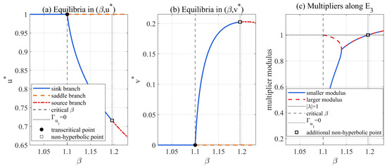
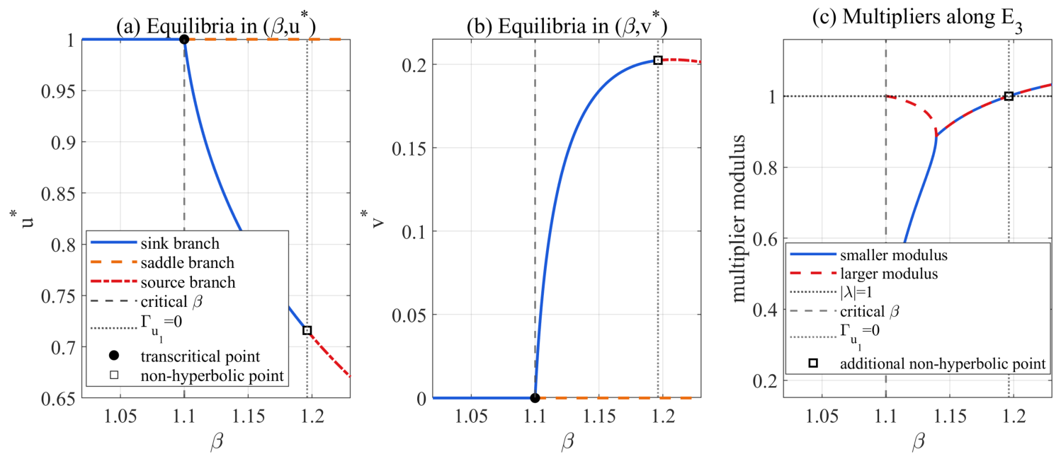
For the transcritical bifurcation at $E_1=(1,0)$, take $\mu =0.30$, $\alpha =1.20$, and $\gamma =0.50$. Then, ${\beta }_1=\gamma (1+\alpha )=1.10$. The boundary branch was sampled at 2101 values on $1.02\le \beta \le 1.23$ ($\Delta \beta ={10}^{-4}$), and the positive branch $E_3$ was sampled at 1600 parameter values on $1.1000001\le \beta \le 1.23$. Figure 1 shows the equilibrium branches, pointwise stability, and multiplier moduli. At $\beta =1.14$, $E_3=(0.824405,0.173083)$ is a sink, in agreement with the Jacobian multipliers.

Figure 1. Equilibrium branches and multiplier moduli associated with the transcritical bifurcation at $E_1$. Colors and line styles identify stability as shown in the legends. The gray dashed and dotted vertical lines mark $\beta ={\beta }_1$ and ${\Gamma }_{u_1}=0$, respectively; the horizontal dotted line in panel (c) marks $\left|\lambda \right|=1$. Filled circles mark the transcritical point, and the open squares in all panels mark the same additional non-hyperbolic point at $\beta \approx 1.19602046$. Overlapping segments have identical coordinates.

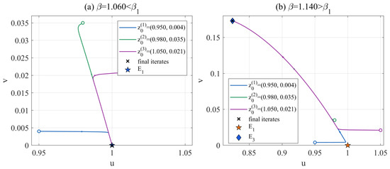
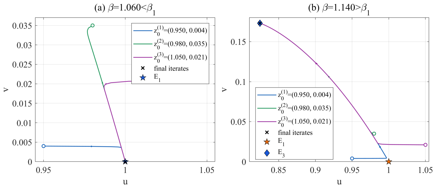
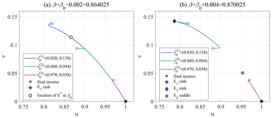
The corresponding phase portraits are shown in Figure 2.

Figure 2. Phase portraits associated with the transcritical bifurcation at $E_1$ for $\beta =1.06<{\beta }_1$ and $\beta =1.14>{\beta }_1$. The three initial conditions in both panels are $(0.950,0.004)$, $(0.980,0.035)$, and $(1.050,0.021)$. Each complete orbit contains 2000 iterates; open circles, arrows, and crosses mark the initial states, forward direction, and final iterates, respectively. The star and diamond mark $E_1$ and $E_3$; overlapping segments share the same forward path.

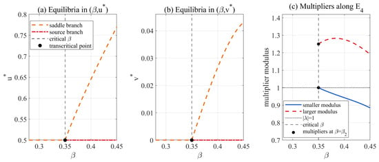
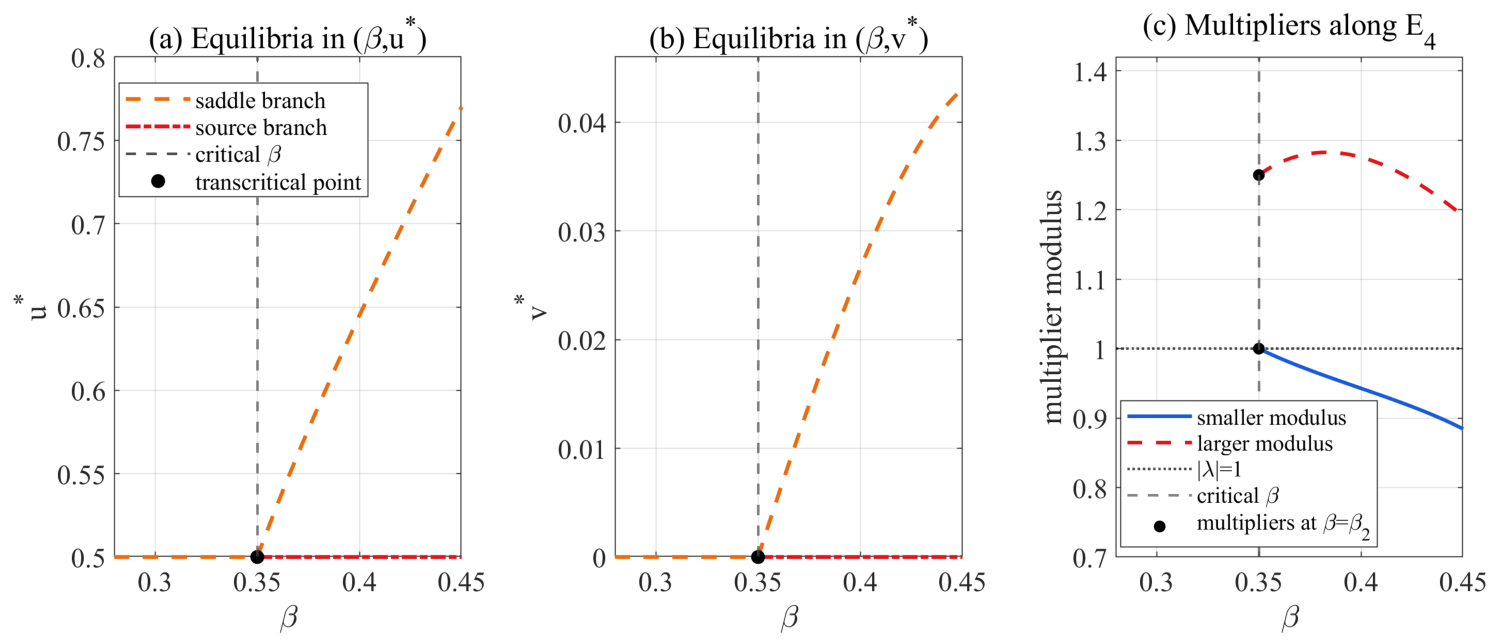
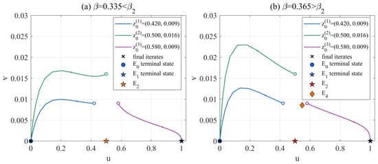
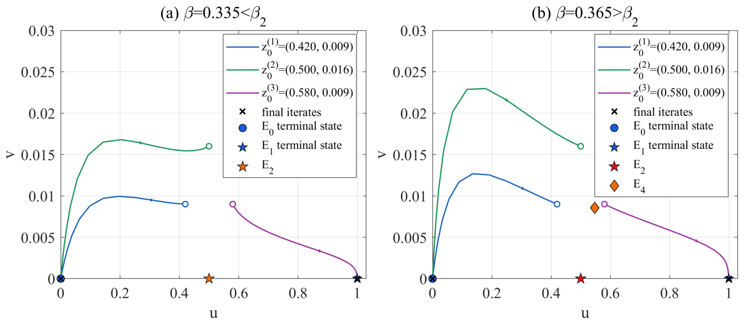
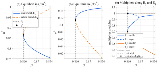
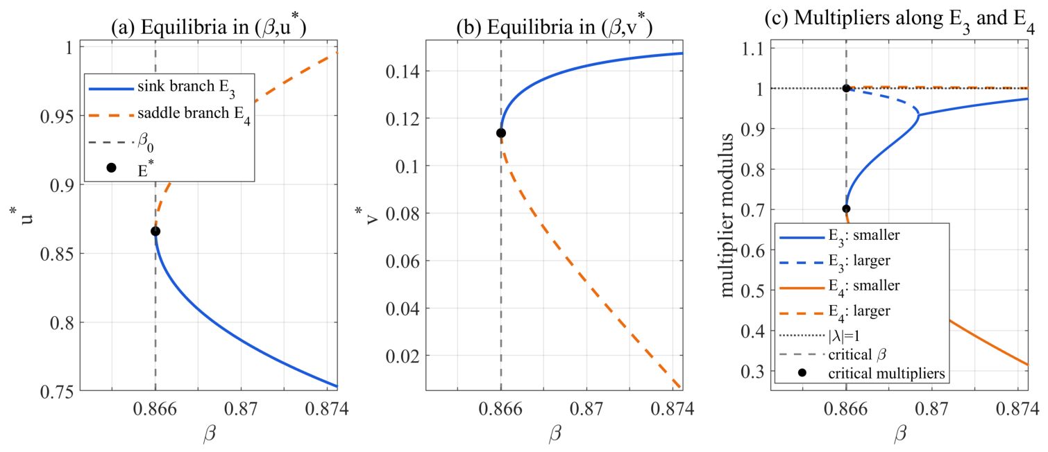
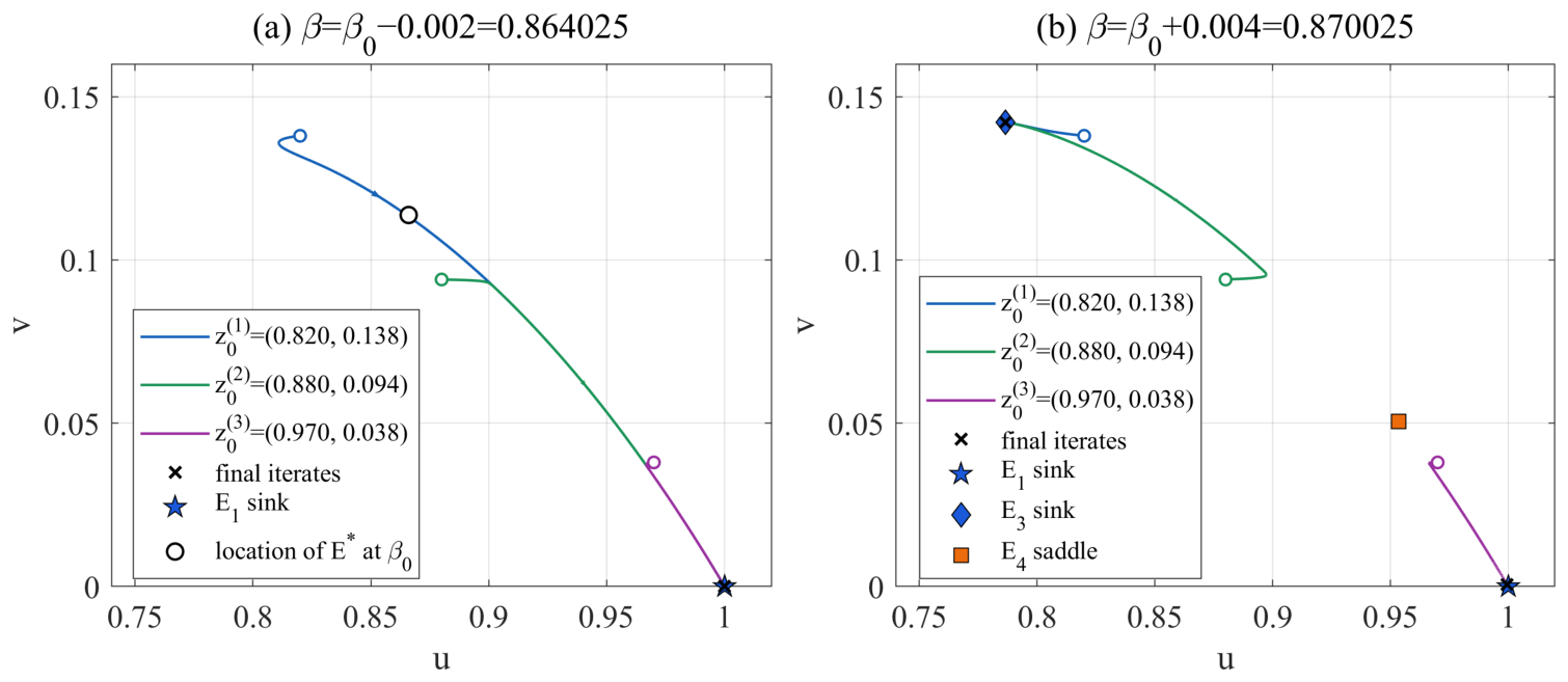
For the transcritical bifurcation at $E_2=(\mu ,0)$, take $\mu =0.50$, $\alpha =0.10$, and $\gamma =0.50$. The critical value is ${\beta }_2=0.35$. The boundary branch was sampled at 1701 values on $0.28\le \beta \le 0.45$ ($\Delta \beta ={10}^{-4}$), while the positive branch $E_4$ was sampled at 1400 parameter values on $0.3500001\le \beta \le 0.45$. Stability was again computed independently at every branch point. The corresponding equilibrium branches and phase portraits are shown in Figure 3 and Figure 4, respectively.

Figure 3. Equilibrium branches and multiplier moduli associated with the transcritical bifurcation at $E_2$. Colors and line styles are identified in the legends; coincident segments have identical coordinates. The filled circles in panel (c) mark both multiplier moduli at ${\beta }_2=0.35$, one of which equals one; no further unit-modulus crossing occurs on the displayed $E_4$ branch.

Figure 4. Phase portraits associated with the transcritical bifurcation at $E_2$ for $\beta =0.335<{\beta }_2$ and $\beta =0.365>{\beta }_2$. The three initial conditions in both panels are $(0.420,0.009)$, $(0.500,0.016)$, and $(0.580,0.009)$. Each complete orbit contains 2000 iterates; open circles, arrows, and crosses mark the initial states, forward direction, and final iterates. The terminal boundary states $E_0$ and $E_1$ are included; coincident endpoint and equilibrium markers indicate convergence.

For the saddle-node bifurcation at $E^{*}$, take $\mu =0.30$, $\alpha =0.75$, and $\gamma =0.50$. These values satisfy the assumptions of Theorem 5. The critical parameter and fixed point are

$${\beta }_0=2\gamma \sqrt{\alpha }=0.8660254038,E^{*}=(0.8660254038,0.1137495374).$$

The two positive branches were each sampled at 1600 parameter values on ${\beta }_0+{10}^{-8}\le \beta \le 0.8745$. The lower branch $E_3$ is a sink, and the upper branch $E_4$ is a saddle in the displayed neighborhood. The equilibrium branches and phase portraits are shown in Figure 5 and Figure 6, respectively.

Figure 5. Saddle-node equilibrium branches and multiplier moduli at $E^{*}$ for ${\beta }_0=0.8660254038$. The blue $E_3$ and orange $E_4$ curves meet at $E^{*}$; this overlap is the saddle-node collision. The filled points in panel (c) mark both multiplier moduli at the collision, one of which equals one.

Figure 6. Phase portraits before and after the saddle-node bifurcation at $E^{*}$, with $\beta ={\beta }_0-0.002$ and $\beta ={\beta }_0+0.004$. The three initial conditions in both panels are $(0.820,0.138)$, $(0.880,0.094)$, and $(0.970,0.038)$. Each complete orbit contains 2000 iterates; open circles, arrows, and crosses mark the initial states, forward direction, and final iterates. The remaining symbols identify the equilibria shown in the legends.

5. Conclusions

In this paper, a discrete predator–prey system with an Allee effect and a Holling-IV functional response is investigated. By applying the semi-discretization method, the corresponding discrete model is derived from the continuous system. Under assumptions $0<\mu <1$, $\alpha >0$, $\beta >0$, and $\gamma >0$, the existence of non-negative fixed points is discussed in detail. In particular, the positive fixed points are characterized by the roots of an auxiliary equation, and their number and distribution are classified according to the relative positions of $\mu$, $\sqrt{\alpha }$, and 1.

Furthermore, the local stability of the boundary fixed points and positive fixed points is analyzed using the eigenvalues of the Jacobian matrix together with the stability criteria for two-dimensional discrete systems. The results show that the boundary fixed point $E_1=(1,0)$ changes from a sink to a saddle as $\beta$ passes through the critical value ${\beta }_1$, while the boundary fixed point $E_2=(\mu ,0)$ changes from a saddle to a source as $\beta$ passes through the critical value ${\beta }_2$. For positive fixed points, different stability conditions are obtained according to whether the fixed point lies on the left branch, the right branch, or the critical position $u=\sqrt{\alpha }$.

Finally, using the center manifold theorem and local bifurcation theory, we establish transcritical bifurcations at $E_1$ when $\beta ={\beta }_1$ and at $E_2$ when $\beta ={\beta }_2$, together with a saddle-node bifurcation at $E^{*}$ when $\beta ={\beta }_0$ under the assumptions of Theorem 5. The numerical simulations illustrate the corresponding local equilibrium branches and stability changes. All conclusions obtained here are local and do not establish global predator persistence, stable coexistence, or ecological transitions for arbitrary initial conditions. From a conservation perspective, the Allee and bifurcation thresholds may serve as qualitative warning indicators for low-density prey recovery, predator invasion, and the possible loss of coexistence states. Nevertheless, because these thresholds arise from a local analysis, they should not be interpreted as global management criteria. The conditions ${\Gamma }_{u_1}=0$ at $E_3$ and $\gamma =\delta$ at $E_4$ only identify possible Neimark–Sacker and flip bifurcations, respectively. Their rigorous study can likewise employ center-manifold and normal-form methods but requires substantially more involved transversality, nonresonance, and higher-order nondegeneracy calculations; it is therefore omitted here. These two positive-equilibrium bifurcations, global boundedness and basin analysis, and the influence of a general step size h are left for future work.

References

- Rosenzweig, M.L.; MacArthur, R.H. Graphical representation and stability conditions of predator–prey interactions. Amer. Natur. 1963, 97, 209–223. [Google Scholar] [CrossRef] [Scilit] [PubMed]
- Sen, M.; Banerjee, M.; Morozov, A. Bifurcation analysis of a ratio-dependent prey–predator model with the Allee effect. Ecol. Complex. 2012, 11, 12–27. [Google Scholar] [CrossRef] [Scilit]
- Ye, Y.; Liu, H.; Wei, Y.; Zhang, K.; Ma, M.; Ye, J. Dynamic study of a predator–prey model with Allee effect and Holling type-I functional response. Adv. Differ. Equ. 2019, 2019, 369. [Google Scholar] [CrossRef] [Scilit]
- Arsie, A.; Kottegoda, C.; Shan, C. High codimension bifurcations of a predator–prey system with generalized Holling type III functional response and Allee effects. J. Dynam. Differ. Equ. 2023, 35, 3355–3380. [Google Scholar] [CrossRef] [Scilit]
- Zeng, Y.; Yu, P. Multistable states in a predator–prey model with generalized Holling type III functional response and a strong Allee effect. Commun. Nonlinear Sci. Numer. Simul. 2024, 131, 107846. [Google Scholar] [CrossRef] [Scilit]
- Seo, G.; Kot, M. A comparison of two predator–prey models with Hollings type I functional response. Math. Biosci. 2008, 212, 161–179. [Google Scholar] [CrossRef] [Scilit] [PubMed]
- Hsu, S.-B.; Hwang, T.-W. Hopf bifurcation analysis for a predator–prey system of Holling and Leslie type. Taiwan. J. Math. 1999, 3, 35–53. [Google Scholar] [CrossRef] [Scilit]
- Wang, L.-L.; Fan, Y.-H.; Li, W.-T. Multiple bifurcations in a predator–prey system with monotonic functional response. Appl. Math. Comput. 2006, 172, 1103–1120. [Google Scholar] [CrossRef] [Scilit]
- AL-Kaff, M.O.; El-Metwally, H.A.; Elabbasy, E.-M.M. Qualitative analysis and phase of chaos control of the predator–prey model with Holling type-III. Sci. Rep. 2022, 12, 20111. [Google Scholar] [CrossRef] [Scilit] [PubMed]
- Shang, Z.; Qiao, Y. Bifurcation analysis of a Leslie-type predator–prey system with simplified Holling type IV functional response and strong Allee effect on prey. Nonlinear Anal. Real. World Appl. 2022, 64, 103453. [Google Scholar] [CrossRef] [Scilit]
- Lv, L.; Li, X. Stability and bifurcation analysis in a discrete predator–prey system of Leslie type with ratio-dependent simplified Holling type IV functional response. Mathematics 2024, 12, 1803. [Google Scholar] [CrossRef] [Scilit]
- Hu, Z.; Teng, Z.; Zhang, L. Stability and bifurcation analysis of a discrete predator–prey model with non-monotonic functional response. Nonlinear Anal. Real. World Appl. 2011, 12, 2356–2377. [Google Scholar] [CrossRef] [Scilit]
- Huang, J.; Liu, S.; Ruan, S.; Xiao, D. Bifurcations in a discrete predator–prey model with nonmonotonic functional response. J. Math. Anal. Appl. 2018, 464, 201–230. [Google Scholar] [CrossRef] [Scilit]
- Yao, W.; Li, X. Bifurcation difference induced by different discrete methods in a discrete predator–prey model. J. Nonlinear Model. Anal. 2022, 4, 64–79. [Google Scholar]
- Carr, J. Applications of Centre Manifold Theory; Springer: New York, NY, USA, 1981. [Google Scholar]
- Guckenheimer, J.; Holmes, P. Nonlinear Oscillations, Dynamical Systems, and Bifurcations of Vector Fields; Springer: New York, NY, USA, 1983. [Google Scholar]
- Kuznetsov, Y.A. Elements of Applied Bifurcation Theory, 4th ed.; Springer: Cham, Switzerland, 2023. [Google Scholar]
- Wiggins, S. Introduction to Applied Nonlinear Dynamical Systems and Chaos, 2nd ed.; Springer: New York, NY, USA, 2003. [Google Scholar]
Disclaimer/Publisher’s Note: The statements, opinions and data contained in all publications are solely those of the individual author(s) and contributor(s) and not of MDPI and/or the editor(s). MDPI and/or the editor(s) disclaim responsibility for any injury to people or property resulting from any ideas, methods, instructions or products referred to in the content. |
© 2026 by the authors. Licensee MDPI, Basel, Switzerland. This article is an open access article distributed under the terms and conditions of the Creative Commons Attribution (CC BY) license.