A Hybrid Index Matrix Framework for Python-Based Modeling, Simulation, and Local One-Step Sensitivity Diagnostics of Bidirectional DC–DC Converters

Abstract

Bidirectional DC–DC converters are key interfaces in battery energy storage systems, electric vehicles, fuel cell vehicles, and DC microgrids, where transparent mathematical models are required for simulation, controller evaluation, and energy-flow analysis. This paper presents a hybrid index matrix framework for the Python-based modeling of a bidirectional buck–boost converter coupled to a first-order Thevenin battery model. In contrast to a classical state-space formulation, the index matrix is used as a label-aware model-assembly layer: component equations are aligned by explicit row and column identifiers and subsequently projected into ordered numerical matrices for solution. Charging, idle, and discharging equations are solved using a fixed-step backward-Euler procedure, and a PI current controller with duty-cycle saturation and anti-windup regulates the power-flow direction. A conventional switched ODE implementation is retained only as a software-level numerical-consistency check between two implementations of the same assumptions; it is not presented as experimental validation or as an independent physical benchmark. For the reported 60 s current profile, the model gives a current RMSE of 0.0863 A and a peak current of 4.3684 A, corresponding to 9.2094% overshoot at the idle-to-discharge transition. The power-integration balance is 1.6091 Wh input, 1.5868 Wh output, and 0.0223 Wh estimated loss under the adopted conduction-oriented loss model. The conditional one-step sensitivity matrices have a spectral radius of 1.00000 in all three modes; the unit eigenvalue is consistent with the slowly varying SOC state, while the remaining electrical eigenvalues lie inside the unit circle. These eigenvalue results are interpreted as local non-divergence diagnostics rather than proof of asymptotic closed-loop or switched-system stability. The framework provides a transparent and reproducible numerical workflow, while experimental validation, detailed switching-level loss modeling, step-size convergence, and formal closed-loop/switched-system stability analysis remain necessary future work.

1. Introduction

The increasing integration of renewable energy sources, battery energy storage systems, electric vehicles, including fuel cell vehicles, and DC microgrids has intensified the need for efficient and flexible power electronic interfaces [1,2,3,4,5,6]. In fuel-cell and hybrid-electric-vehicle architectures, DC–DC converters are commonly required to interface fuel-cell stacks, batteries, supercapacitors, and DC-link buses under variable power-flow conditions. Bidirectional DC–DC converters are essential components in these systems because they enable controlled energy exchange between batteries, DC buses, supercapacitors, renewable generators, and electrical loads [7,8,9]. Depending on the operating requirements, such converters must support battery charging, battery discharging, voltage regulation, current limitation, idle operation, and reversal of the power-flow direction [10,11]. Their design therefore requires mathematical and computational models capable of representing operating modes, non-ideal electrical components, battery dynamics, control functions, and operating constraints within a unified framework [12,13].

Power electronic converters are commonly modeled using switched differential equations, state-space representations, averaged models, or detailed circuit-oriented simulation environments [14,15]. Switched differential models provide a physically interpretable description of the converter but require a separate equation set for each switching configuration [16]. Their formulation becomes increasingly complex when semiconductor non-idealities, parasitic component parameters, battery dynamics, and digital controllers are considered simultaneously [17,18]. State-space models offer a compact representation suitable for control-system analysis; however, the system matrices are topology-dependent and must generally be derived for every operating mode [19,20]. Averaged models reduce the computational burden and are widely applied in controller design, but they do not resolve individual switching events, discontinuous-conduction effects, or high-frequency parasitic phenomena [21,22].

Detailed circuit simulation tools provide comprehensive component libraries and numerical solvers, but repeated simulations may require considerable computational resources [23,24]. This limitation becomes particularly important in model-based design, where large parameter spaces must be explored, and thousands of simulations may be required for controller tuning, sensitivity studies, multi-objective optimization, and uncertainty analysis [25,26]. A suitable modeling framework should therefore combine physical interpretability, computational efficiency, automated model assembly, and compatibility with numerical optimization and stability-analysis tools.

Recent bidirectional converter studies cover wide-bandgap devices, battery emulation, V2G interfaces, energy-management strategies, multiport structures, and controller design for topology-specific applications [27,28,29,30,31,32,33,34,35,36,37,38]. These studies underscore that converter equations, controller states, and parameter sets are commonly tailored to a particular circuit and operating regime. Matrix-based and model-depth investigations further show that the choice of representation affects transparency, computational burden, and suitability for repeated analysis [39,40]. The present work addresses a narrower methodological question: how component and mode equations can be assembled through explicit labels before projection into the ordered matrices required by conventional numerical solvers.

Index matrices extend the functionality of classical matrices by assigning explicit indices to rows and columns. These indices may represent electrical variables, component identifiers, circuit equations, discrete control signals, or operating modes [41,42]. As a result, component equations can be combined according to their physical meaning without requiring a fixed global ordering of the variables. Index matrices with real-valued elements have previously been used to describe resistors, inductors, capacitors, voltage sources, semiconductor switches, electrical nodes, circuit loops, and control blocks within a common discrete-time formulation [43,44].

Earlier work demonstrated software-oriented assembly of power-electronic component, interconnection, and controller equations through real-valued index matrices [43]. The resulting systems are converted to ordered algebraic equations and solved at consecutive time instants, providing a reusable model-construction layer for several converter structures.

A subsequent study applied the approach to a buck DC–DC converter with non-ideal components and a proportional–integral controller and coupled the model to repeated parameter-space calculations [44]. That study remained unidirectional and considered a more limited set of operating modes; the present work extends the formulation to a battery-coupled bidirectional case.

Bidirectional converters introduce additional mathematical and computational challenges. Their operating topology changes not only according to the instantaneous semiconductor switching signals but also according to the required direction of power transfer. The converter may operate in charging, discharging, freewheeling, idle, or transitional states. Some theoretical switching combinations may be physically inadmissible because they can produce shoot-through conditions, uncontrolled current paths, or electrical configurations that violate the operating constraints. A systematic procedure is therefore required to generate the possible switching modes, determine their corresponding mathematical models, and exclude invalid configurations before the simulation is performed.

The presence of a battery introduces further dynamic states. The battery terminal voltage cannot generally be represented by an ideal constant voltage source because it depends on the state of charge, current direction, internal resistance, polarization effects, temperature, and operating history. Even when a first-order equivalent-circuit model is employed, its dynamic equations must be coupled with the converter inductor current, DC-link voltage, switching state, and control variables. This coupling converts the complete system into a hybrid dynamical model containing both continuous electrical quantities and discrete operating decisions.

Hybrid converter systems are often represented by a family of mode-dependent state-space equations. Although this representation is appropriate for numerical solution and control analysis, manual derivation and reordering become labor-intensive when the power stage, battery, supervisory logic, and digital controller are developed as separate model blocks. This fragmented treatment also increases the risk of inconsistent variable ordering and sign conventions across charging, idle, and discharging modes.

The index matrix approach used in this work does not replace classical state-space analysis. Its role is to provide a label-aware assembly layer in which rows identify equations and columns identify physical variables, states, inputs, or constants. Component equations are first combined by these symbolic identifiers; the assembled indexed system is then projected into an ordered classical matrix for solution with standard numerical linear-algebra routines. The incremental contribution is therefore the reproducible assembly and management of the multi-mode converter–battery–controller model, rather than a new state-space stability theorem.

Local dynamic behavior is examined through a one-step finite-difference matrix at representative fixed-mode operating points. Because this diagnostic is local and the controller integral memory is not included as an independent state in the reported four-state vector, its eigenvalues must not be interpreted as a complete closed-loop or switched-system stability proof. A formal assessment would require an augmented closed-loop state, operating-point coverage, switching-sequence analysis, and, where appropriate, Lyapunov-based arguments.

Component tolerances and operating uncertainty remain important for hardware-oriented design. However, the present paper evaluates a nominal parameter set only. Sensitivity, uncertainty, and robust multi-objective optimization are therefore identified as follow-up studies rather than presented as completed contributions.

Python provides an open environment for the proposed workflow. NumPy is used for indexed-array operations and linear-system solution, pandas for data export, and matplotlib for visualization. The present implementation is intentionally limited to model assembly, fixed-step simulation, post-processing, and local one-step diagnostics; optimization and convex stability tools are not required for the results reported here.

In the present study, a custom index matrix data structure stores explicit row and column identifiers together with the corresponding numerical coefficients. The implemented workflow supports label-consistent addition, projection, conversion to an ordered classical matrix, and fixed-step solution of the mode-dependent algebraic systems. Reusable component-level models are provided for the inductor, capacitor, source, simplified semiconductor switches, electrical interconnections, first-order Thevenin battery, supervisory logic, and PI controller. The same workflow performs metric extraction, energy-flow post-processing, data export, and local one-step finite-difference diagnostics.

The reference switched ODE implementation is used only as a software-level numerical-consistency check. It represents the same converter, battery, controller, mode logic, and sign conventions in conventional differential-equation form. Agreement can reveal coding or assembly inconsistencies between the two implementations, but it cannot establish physical accuracy because both descriptions share the same modeling assumptions.

Accordingly, the study focuses on label-aware model assembly, Python-based fixed-step simulation, performance-metric evaluation, conduction-oriented energy accounting, and conditional one-step diagnostics for three fixed operating modes. Experimental validation, comparison with detailed switching-level software, step-size convergence, uncertainty analysis, robust optimization, and formal switched-system stability are outside the present scope and are stated explicitly as future work.

Despite previous applications of index matrices to power-electronic systems, several gaps motivate the present work. First, the extension from a unidirectional converter to a battery-coupled bidirectional structure requires explicit handling of charging, idle, and discharging operation. Second, converter, battery, controller, and supervisory equations must be assembled without relying on a fragile global variable order. Third, the relationship between the indexed assembly and the downstream ordered numerical matrices must be made explicit. Fourth, the limits of a local one-step finite-difference diagnostic must be reported transparently. Finally, a compact Python workflow integrating these elements has not been demonstrated sufficiently for the considered bidirectional case.

The objective of this study is therefore to develop a Python-based hybrid index matrix framework for the unified assembly and simulation of a bidirectional DC–DC converter connected to a battery energy storage system. The framework combines the power converter, non-ideal passive components, simplified switch constraints, battery dynamics, digital current controller, and supervisory mode-selection logic in a common indexed representation. Mode-dependent systems are generated for charging, idle, and discharging operation and solved with a fixed-step implicit procedure. The resulting data are used to evaluate current tracking, DC-link voltage deviation, power flow, physically scaled SOC evolution, conduction-oriented energy accounting, and conditional one-step sensitivity diagnostics.

Compared with previous index matrix studies focused mainly on unidirectional converter structures, the present work advances the methodology in six specific ways. First, charging, idle, and discharging modes are represented within one indexed computational structure. Second, a first-order Thevenin battery model is coupled to the converter through indexed state variables, including open-circuit voltage, ohmic drop, polarization dynamics, and SOC evolution. Third, supervisory mode selection is based on the current-reference sign and SOC limits. Fourth, a mode-dependent coefficient enforces a consistent bidirectional current sign convention. Fifth, the assembly rule distinguishes a genuinely absent coefficient from a conflicting duplicate row–column label. Sixth, the Python workflow integrates fixed-step solution, PI current control, quantitative metrics, energy post-processing, and a clearly delimited one-step finite-difference diagnostic. Thus, the index matrix acts as a label-aware assembly mechanism, whereas classical ordered matrices remain the downstream representation used by conventional solvers and eigenvalue routines.

The main contributions of this study are summarized as follows:

• A hybrid index matrix model is developed for a bidirectional buck–boost DC–DC converter connected to a battery energy storage system, covering charging, idle, and discharging operation.
• A first-order Thevenin battery model is integrated into the indexed formulation, including open-circuit voltage, ohmic resistance, polarization dynamics, SOC evolution, and charge/discharge efficiencies.
• A label-aware Python procedure assembles the mode-dependent equation systems by symbolic row and column identifiers and projects them into ordered numerical matrices for fixed-step solution.
• Supervisory logic selects charging, idle, or discharging according to the current-reference sign and SOC limits, while a mode coefficient enforces a consistent bidirectional current convention.
• A PI current controller with duty-cycle saturation and anti-windup is incorporated to regulate the current magnitude in both power-flow directions.
• The deterministic simulation is quantified using current-error metrics, DC-link deviation, physically scaled SOC, power integration, and conduction-oriented loss indicators.
• A conditional one-step finite-difference diagnostic is constructed for representative charging, idle, and discharging operating points. The resulting matrices, eigenvalues, and spectral radii are reported as local sensitivity indicators, not as proof of asymptotic closed-loop or switched-system stability.
• The complete workflow exports numerical data and publication-oriented figures without requiring proprietary power-electronics simulation software.

2. Mathematical Framework and Numerical Formulation

2.1. Real-Valued Index Matrix Representation

In a conventional matrix, the interpretation of each element depends on its numerical position. In an index matrix, every row and column is associated with an explicit symbolic index. Each real-valued index matrix is defined by

$$F=\langle R_F,C_F,a_F\rangle ,\hspace{1em}\hspace{1em}{a}_F: R_F\times C_F\to ℝ.$$

(1)

Here, $R_F$ and $C_F$ are the row- and column-index sets, respectively, and $a_F: R_F\times C_F\to ℝ$ maps each indexed pair $\left(r,c\right)$ to a real coefficient. For the ordered index tuples

$$R_F=\left(r_1,r_2,\dots ,r_m\right),\hspace{1em}\hspace{1em}{C}_F=\left(c_1,c_2,\dots ,c_n\right).$$

(2)

The corresponding coefficient array is defined by

$${\left[A_F\right]}_{ij}=a_F\left(r_i,c_j\right),\hspace{1em}\hspace{1em}i=1,\dots ,m,\hspace{1em}j=1,\dots ,n.$$

(3)

In the present paper, each row index represents an equation, whereas each column index identifies a physical variable, state quantity, control signal, or constant term. This enables the electrical-component, circuit-constraint, battery, and controller equations to be assembled according to physical meaning. For example, $i_{L,k}$ denotes the inductor current at the current time step, while $i_{L,k-1}$ denotes its value at the preceding step. The active operating mode can therefore be changed without manually reordering the matrices.

2.2. Index Matrix Addition

Let two index matrices be given by

$$F_1=\langle R_{F_1},C_{F_1},a_{F_1}\rangle ,\hspace{1em}\hspace{1em}{F}_2=\langle R_{F_2},C_{F_2},a_{F_2}\rangle .$$

(4)

Their addition is denoted by

$$F=\langle R_F,C_F,a_F\rangle =F_1\oplus F_2.$$

(5)

with resulting row- and column-index sets

$$R_F=R_{F_1}{\displaystyle \cup }{R}_{F_2},\hspace{1em}\hspace{1em}{C}_F=C_{F_1}{\displaystyle \cup }{C}_{F_2}.$$

(6)

For arbitrary $r\in R_F$ and $c\in C_F$, let $a_{F_{\nu }}^0\left(r,c\right)$ equal $a_{F_{\nu }}\left(r,c\right)$ when the key $\left(r,c\right)$ exists in $F_{\nu }$ and equal zero otherwise. The resulting coefficient is

$$a_F\left(r,c\right)=a_{F_1}^0\left(r,c\right)+a_{F_2}^0\left(r,c\right),\hspace{1em}\hspace{1em}r\in R_F,|c\in C_F.$$

(7)

An absent coefficient is assigned the value zero only after the symbolic row and column identifiers have been matched. Index matrix addition therefore does not rely on numerical position, and no positional shifting of terms is permitted.

During assembly, each coefficient is addressed by the key (row label, column label). A missing key is initialized to zero. Contributions assigned to an existing key may be accumulated only when they refer to the same physical equation and the same physical variable with compatible units and sign conventions; otherwise, the assembly is classified as a conflict and the model construction must stop rather than silently combine the terms.

This rule is applied when component-level equations for inductors, capacitors, sources, switches, battery elements, electrical nodes, loops, and control blocks are combined. Unique equation labels and consistent variable labels are therefore prerequisites for model assembly. The rule prevents unintended merging of unrelated quantities and addresses row/column mismatch at assembly time.

Index matrix addition is consequently a label-consistent assembly operation, not a blind numerical sum. The zero convention applies only to genuinely absent terms in otherwise compatible indexed equations.

2.3. Projection and Conversion to a Classical Matrix

Before numerical solution, the assembled index matrix is projected onto selected sets of equations and unknown variables to a classical matrix:

$$F_P=\mathrm{proj}\left(F,R_P,C_P\right)=\mathrm{proj}\left(\langle R_F,C_F,a_F\rangle ,R_P,C_P\right).$$

(8)

Here

$$R_P=\left(r_1^{\prime },r_2^{\prime },\dots ,r_v^{\prime }\right),\hspace{1em}\hspace{1em}{C}_P=\left(c_1^{\prime },c_2^{\prime },\dots ,c_w^{\prime }\right).$$

(9)

are ordered index sets under condition

$$\left\{r_1^{\prime },r_2^{\prime },\dots ,r_v^{\prime }\right\}\subseteq R_F,\hspace{1em}\hspace{1em}\left\{c_1^{\prime },c_2^{\prime },\dots ,c_w^{\prime }\right\}\subseteq C_F.$$

(10)

The corresponding classical numerical matrix is

$$A=\left[\begin{array}{cccc}{a}_F\left(r_1^{\prime },c_1^{\prime }\right)& a_F\left(r_1^{\prime },c_2^{\prime }\right)& \dots & a_F\left(r_1^{\prime },c_w^{\prime }\right)\\ a_F\left(r_2^{\prime },c_1^{\prime }\right)& a_F\left(r_2^{\prime },c_2^{\prime }\right)& \dots & a_F\left(r_2^{\prime },c_w^{\prime }\right)\\ ⋮& ⋮& \ddots & ⋮\\ a_F\left(r_v^{\prime },c_1^{\prime }\right)& a_F\left(r_v^{\prime },c_2^{\prime }\right)& \dots & a_F\left(r_v^{\prime },c_w^{\prime }\right)\end{array}\right].$$

(11)

Thus, symbolic indices are retained during model construction, whereas conventional numerical linear-algebra routines are employed during the solution stage.

2.4. Discrete-Time Formulation

The proposed model is formulated in discrete time using a constant integration interval:

$$\Delta t=t_k-t_{k-1}>0,\hspace{1em}\hspace{1em}\Delta t=\mathrm{constant}.$$

(12)

The dynamic component equations are discretized by the backward Euler method:

$${{\displaystyle \frac{dx\left(t\right)}{dt}}|}_{t=t_k}\approx {\displaystyle \frac{x_k-x_{k-1}}{\Delta t}}.$$

(13)

This implicit approximation converts the differential equations into algebraic equations that are solved at every simulation step.

2.5. Inductor Model

For an inductor with inductance $L$ and series resistance $R_L$, the continuous-time equation is

$$u_L\left(t\right)=L{\displaystyle \frac{d{i}_L\left(t\right)}{dt}}+R_L\hspace{0.17em}{i}_L\left(t\right).$$

(14)

After applying the backward Euler approximation,

$$u_{L,k}={\displaystyle \frac{L}{\Delta t}}\left(i_{L,k}-i_{L,k-1}\right)+R_L\hspace{0.17em}{i}_{L,k}.$$

(15)

An algebraic equation included in the index matrix is

$$-u_{L,k}+\left({\displaystyle \frac{L}{\Delta t}}+R_L\right)i_{L,k}-{\displaystyle \frac{L}{\Delta t}}{i}_{L,k-1}=0.$$

(16)

and its corresponding index matrix is

$$\left(a_L\left(e_L,u_{L,k}\right),a_L\left(e_L,i_{L,k}\right),a_L\left(e_L,i_{L,k-1}\right)\right)=\left(-1,{\displaystyle \frac{L}{\Delta t}}+R_L,-{\displaystyle \frac{L}{\Delta t}}\right).$$

(17)

2.6. Capacitor Model

For a capacitor with capacitance $C$ and equivalent series resistance $R_C$, the terminal voltage is

$$u_C\left(t\right)=u_{C,0}\left(t\right)+R_C\hspace{0.17em}{i}_C\left(t\right).$$

(18)

where the ideal capacitor current is

$$i_C\left(t\right)=C{\displaystyle \frac{d{u}_{C,0}\left(t\right)}{dt}}.$$

(19)

After discretization,

$$i_{C,k}={\displaystyle \frac{C}{\Delta t}}\left[\left(u_{C,k}-u_{C,k-1}\right)-R_C\left(i_{C,k}-i_{C,k-1}\right)\right].$$

(20)

and the resulting algebraic equation is

$${\displaystyle \frac{C}{\Delta t}}{u}_{C,k}-\left(1+{\displaystyle \frac{C{R}_C}{\Delta t}}\right)i_{C,k}-{\displaystyle \frac{C}{\Delta t}}{u}_{C,k-1}+{\displaystyle \frac{C{R}_C}{\Delta t}}{i}_{C,k-1}=0.$$

(21)

The capacitor index matrix is

$$\begin{array}{c}\left(a_C\left(e_C,u_{C,k}\right),a_C\left(e_C,i_{C,k}\right),a_C\left(e_C,u_{C,k-1}\right),a_C\left(e_C,i_{C,k-1}\right)\right)\\ \hspace{1em}\hspace{1em}\hspace{1em}\hspace{1em}=\left({\displaystyle \frac{C}{\Delta t}},-1-{\displaystyle \frac{C{R}_C}{\Delta t}},-{\displaystyle \frac{C}{\Delta t}},{\displaystyle \frac{C{R}_C}{\Delta t}}\right).\end{array}$$

(22)

2.7. Resistor Model

The resistor equation is

$$u_{R,k}=R\hspace{0.17em}{i}_{R,k}.$$

(23)

Its corresponding index matrix is

$$\left(a_R\left(e_R,u_{R,k}\right),a_R\left(e_R,i_{R,k}\right)\right)=\left(-1,R\right).$$

(24)

2.8. Voltage-Source Model

A non-ideal voltage source with electromotive force $E$ and internal resistance $R_E$ is considered. With $i_{E,k}$ defined as positive when the source delivers current to the external circuit, its terminal voltage is

$$u_{E,k}=E-R_E\hspace{0.17em}{i}_{E,k}.$$

(25)

Its index matrix is

$$\left(a_E\left(e_E,u_{E,k}\right),a_E\left(e_E,i_{E,k}\right),a_E\left(e_E,1\right)\right)=\left(-1,-R_E,E\right).$$

(26)

The auxiliary column indexed by 1 represents a constant term.

2.9. Semiconductor Switch Representation

The semiconductor switch is represented by a simplified algebraic model with two operating states: the conducting and blocking states. This representation is used to construct the mode-dependent index matrix equations and to demonstrate how switching conditions can be included in the proposed indexed formulation.

In the conducting state, the switch is modeled by its on-state resistance:

$$u_{S,k}=R_{\mathrm{on}}{i}_{S,k}.$$

(27)

where $R_{\mathrm{on}}$ is the on-state resistance. The corresponding indexed coefficient row is

$$\left(a_{S,\mathrm{on}}\left(e_{S,\mathrm{on}},u_{S,k}\right),a_{S,\mathrm{on}}\left(e_{S,\mathrm{on}},i_{S,k}\right)\right)=\left(-1,R_{\mathrm{on}}\right).$$

(28)

In the blocking state, the switch current is forced to zero:

$$i_{S,k}=0.$$

(29)

The corresponding index matrix is

$$a_{S,\mathrm{off}}\left(e_{S,\mathrm{off}},i_{S,k}\right)=1.$$

(30)

The active switch equation is selected based on the switching variable s_k ∈ {0,1}, where s_k = 1 denotes the conducting state and s_k = 0 denotes the blocking state.

It should be emphasized that this switch representation is a first-order algebraic approximation. It is introduced to support the construction of the index matrix model and the numerical simulation of the converter operating modes. The model does not include switching transients, parasitic capacitances, reverse-recovery effects, gate-drive losses, temperature-dependent semiconductor parameters, or switching-frequency-dependent losses.

Therefore, the switch equations used in the present work should not be interpreted as a detailed semiconductor device model. They provide a compact representation of the conducting and blocking constraints required for the mode-dependent converter equations. A more detailed implementation may replace this simplified switch row with an extended semiconductor model including conduction losses, switching losses, diode recovery effects, parasitic elements, and thermal dependencies.

This clarification is important for interpreting the efficiency and loss results presented later. Because the switch model includes only simplified resistive behavior, the reported efficiency is an estimated conduction-oriented internal-model indicator, not a prediction of the full hardware efficiency of a real converter.

2.10. Circuit Interconnection Equations

Kirchhoff’s current law for node n is expressed as

$${\displaystyle \sum }_{j\in \mathcal{N}\left(n\right)}{\sigma }_{jn}{i}_{jn}=0,\hspace{1em}\hspace{1em}{\sigma }_{jn}\in \left\{-1,+1\right\}.$$

(31)

Here, $j\in \mathcal{N}\left(n\right)$ denotes a node adjacent to $n$. The incidence factor is ${\sigma }_{jn}=+1$ for a branch current directed into node $n$ and ${\sigma }_{jn}=-1$ for a current directed out of the node.

Kirchhoff’s voltage law for loop l is

$${\displaystyle \sum }_{b\in ℬ\left(l\right)}{\sigma }_{bl}{u}_{bl}=0,\hspace{1em}\hspace{1em}{\sigma }_{bl}\in \left\{-1,+1\right\}.$$

(32)

Here, $b\in ℬ\left(l\right)$ denotes a branch in loop $l$. The orientation factor is ${\sigma }_{bl}=+1$ when the branch-voltage orientation agrees with the loop orientation and ${\sigma }_{bl}=-1$ otherwise.

The node and loop index matrices are denoted by $F_n$ and $F_l$, respectively, while $F_c$ denotes the index matrix of component $c$.

The complete system index matrix is assembled as

$$F_{\mathrm{sys}}=F_{\mathrm{comp}}\oplus F_{\mathrm{node}}\oplus F_{\mathrm{loop}}.$$

(33)

The individual parts are

$$F_{\mathrm{comp}}={\oplus }_c{F}_c,\hspace{1em}\hspace{1em}{F}_{\mathrm{node}}={\oplus }_n{F}_n,\hspace{1em}\hspace{1em}{F}_{\mathrm{loop}}={\oplus }_l{F}_l.$$

(34)

2.11. Operating Modes

Three principal operating modes are considered:

$$m\in ℳ=\left\{\mathrm{charge},\mathrm{idle},\mathrm{discharge}\right\}.$$

(35)

For each operating mode, a discrete system with a state vector

$$x_k={\left[\begin{array}{cccc}{i}_{L,k}& u_{\mathrm{DC},k}& u_{p,k}& SO{C}_k\end{array}\right]}^{\mathrm{T}}.$$

(36)

Here, $i_{L,k}$ is the inductor-current magnitude, $u_{\mathrm{DC},k}$ is the DC-link voltage, $u_{p,k}$ is the battery polarization voltage, and $SO{C}_k$ is the battery state of charge at time step $k$.

2.12. Battery Model

The battery is represented by a first-order Thevenin equivalent circuit containing an open-circuit voltage source, an ohmic resistance $R_0$, and a polarization branch $R_p$ − $C_p$. The terminal voltage is

$$u_{\mathrm{bat}}=u_{\mathrm{oc}}\left(\mathit{SOC}\right)+R_0\hspace{0.17em}{i}_{\mathrm{bat}}+u_p.$$

(37)

The adopted sign convention is $i_{\mathrm{bat}}>0$ during charging and $i_{\mathrm{bat}}<0$ during discharging. The polarization-voltage dynamics are

$${\displaystyle \frac{d{u}_p}{dt}}=-{\displaystyle \frac{u_p}{R_p{C}_p}}+{\displaystyle \frac{i_{\mathrm{bat}}}{C_p}}.$$

(38)

Using backward Euler discretization gives

$$\left({\displaystyle \frac{1}{\Delta t}}+{\displaystyle \frac{1}{R_p{C}_p}}\right)u_{p,k+1}-{\displaystyle \frac{i_{\mathrm{bat},k+1}}{C_p}}={\displaystyle \frac{u_{p,k}}{\Delta t}}.$$

(39)

The battery state of charge is calculated by Coulomb counting. During charging,

$$SO{C}_{k+1}=SO{C}_k+{\displaystyle \frac{{\eta }_{\mathrm{ch}}\Delta t}{3600Q_n}}{i}_{\mathrm{bat},k+1}.$$

(40)

During discharging,

$$SO{C}_{k+1}=SO{C}_k+{\displaystyle \frac{\Delta t}{3600{\eta }_{\mathrm{dis}}{Q}_n}}{i}_{\mathrm{bat},k+1}.$$

(41)

For an optional visualization only, the physical SOC increment $\Delta SO{C}_k^{\left(\mathrm{phys}\right)}$ may be scaled by a factor $K_{\mathit{SOC}}$:

$$SO{C}_{k+1}^{\left(\mathrm{vis}\right)}=SO{C}_k+K_{\mathit{SOC}}\hspace{0.17em}\Delta SO{C}_k^{\left(\mathrm{phys}\right)}.$$

(42)

All numerical results and the SOC curve reported in this paper use

$$K_{\mathit{SOC}}=1.$$

(43)

Values $K_{\mathit{SOC}}>1$ are not used in the Results section and must not be interpreted as physical Coulomb-counting results.

2.13. PI Current Controller

The current-control error is defined as

$$e_{i,k}=\left|i_{\mathrm{ref},k}\right|-i_{L,k}.$$

(44)

The integral contribution is updated using a clamping anti-windup rule:

$$I_k=\mathrm{sat} \left(I_{k-1}+K_i{e}_{i,k}\Delta t,-I_{\max },I_{\max }\right).$$

(45)

For charging operation, the preliminary duty-cycle command is

$$d_k^{\star }=d_{\mathrm{ff},k}+K_p{e}_{i,k}+I_k.$$

(46)

For discharging operation,

$$d_k^{\star }=d_{\mathrm{ff},k}-K_p{e}_{i,k}-I_k.$$

(47)

The feedforward component is calculated as

$$d_{\mathrm{ff},k}={\displaystyle \frac{u_{\mathrm{oc},k}}{u_{\mathrm{DC},k}}}.$$

(48)

The applied duty cycle is constrained by

$$d_k=\mathrm{sat}\left(d_k^{\star },d_{\min },d_{\max }\right)=\{\begin{array}{ll}{d}_{\min },\hfill & d_k^{\star }<d_{\min },\hfill \\ d_k^{\star },\hfill & d_{\min }\le d_k^{\star }\le d_{\max },\hfill \\ d_{\max },\hfill & d_k^{\star }>d_{\max }.\hfill \end{array}$$

(49)

Equation (45) limits the integral contribution to $\left[-I_{\max },I_{\max }\right]$, while Equation (49) separately constrains the applied duty cycle. This prevents continued integral growth when the actuator is saturated.

2.14. Reference Switched ODE Model for Numerical Consistency Checking

For numerical-consistency checking, a reference switched ODE model is formulated using the same physical assumptions as the index matrix model. Its purpose is limited to software-level numerical-consistency checking: it tests whether the indexed assembly reproduces the intended converter, battery, controller, and mode equations in a conventional implementation. It is not an experimental validation of the physical converter.

The reference model is written as

$$\dot{x}\left(t\right)=f_m \left(x\left(t\right),u\left(t\right),t\right).$$

(50)

The continuous state vector is

$$x\left(t\right)={\left[\begin{array}{cccc}{i}_L\left(t\right)& u_{\mathrm{DC}}\left(t\right)& u_p\left(t\right)& \mathit{SOC}\left(t\right)\end{array}\right]}^{\mathrm{T}}.$$

(51)

Here, $i_L\left(t\right)$ is the inductor-current magnitude, $u_{\mathrm{DC}}\left(t\right)$ is the DC-link voltage, $u_p\left(t\right)$ is the battery polarization voltage, and $\mathit{SOC}\left(t\right)$ is the battery state of charge.

The reference-model operating mode is selected from the current-reference sign together with the SOC limits:

$$m\left(t\right)=\{\begin{array}{ll}\mathrm{charge},\hfill & i_{\mathrm{ref}}\left(t\right)>0\left|\mathrm{and}\right|\mathit{SOC}\left(t\right)<SO{C}_{\max },\hfill \\ \mathrm{discharge},\hfill & i_{\mathrm{ref}}\left(t\right)<0\left|\mathrm{and}\right|\mathit{SOC}\left(t\right)>SO{C}_{\min },\hfill \\ \mathrm{idle},\hfill & \mathrm{otherwise}.\hfill \end{array}$$

(52)

The reference ODE implementation uses the same sign convention, battery equivalent-circuit equations, PI current-control law, and supervisory mode logic as the index matrix formulation. The equations are coded separately in conventional switched differential-equation form so that discrepancies caused by indexing, assembly, or sign errors can be detected. The reference is independent at the software-implementation level, but not at the level of physical assumptions.

The comparison should therefore be interpreted only as a numerical-consistency check between two implementations of the same assumed model. Agreement does not demonstrate correspondence with a real converter, experimentally identified battery, or switching-level semiconductor behavior.

Physical validation would require laboratory measurements, experimentally identified parameters, measured loss data, or comparison with a detailed switching-level benchmark. These activities are outside the present scope and are identified as necessary future work.

3. Bidirectional Converter, Battery, and Control System Model

3.1. Converter Structure and Operating Principle

The investigated system is a bidirectional buck–boost DC–DC converter connected between a DC source/load side and a battery energy storage system. Charging transfers energy from the DC bus to the battery, discharging transfers energy from the battery to the DC bus, and the idle state represents a zero reference or an active SOC constraint. The discrete operating mode is selected as

$$m_k=\{\begin{array}{ll}\mathrm{charge},\hfill & i_{\mathrm{ref},k}>0\left|\mathrm{and}\right|SO{C}_k<SO{C}_{\max },\hfill \\ \mathrm{discharge},\hfill & i_{\mathrm{ref},k}<0\left|\mathrm{and}\right|SO{C}_k>SO{C}_{\min },\hfill \\ \mathrm{idle},\hfill & \mathrm{otherwise}.\hfill \end{array}$$

(53)

The upper SOC limit disables charging and the lower SOC limit disables discharging; both constraints are included explicitly in Equation (53).

3.2. Charge, Idle, and Discharge Modes

The battery-current sign is represented by the mode-dependent coefficient ${\beta }_m$, defined as

$${\beta }_m=\{\begin{array}{ll}+1,\hfill & m=\mathrm{charge},\hfill \\ 0,\hfill & m=\mathrm{idle},\hfill \\ -1,\hfill & m=\mathrm{discharge}.\hfill \end{array}$$

(54)

The battery current is related to the inductor-current magnitude by

$$i_{\mathrm{bat},k}={\beta }_m{i}_{L,k}.$$

(55)

Thus, positive battery current denotes charging and negative battery current denotes discharging. The duty cycle $d_k$ controls the averaged converter-side voltage, and the applied command is constrained by

$$d_{\min }\le d_k\le d_{\max }.$$

(56)

3.3. DC-Link Voltage Equation

The DC-link voltage is determined by the balance between the source current, load current, converter bus current, and DC-link capacitor current. The source current is modeled as

$$i_{s,k}={\displaystyle \frac{U_s-u_{\mathrm{DC},k}}{R_s}}.$$

(57)

where $U_s$ is the source electromotive force and $R_s$ is the equivalent series resistance. The minus sign in Equation (57) follows from defining $i_{s,k}$ as current delivered by the source.

The load current is

$$i_{\mathrm{load},k}={\displaystyle \frac{u_{\mathrm{DC},k}}{R_{\mathrm{load}}}}.$$

(58)

The current exchanged by the converter with the DC bus is approximated as

$$i_{\mathrm{conv},k}={\beta }_m{d}_k{i}_{L,k}.$$

(59)

Using backward Euler discretization, the DC-link capacitor equation can be written in the form

$${\displaystyle \frac{C_{\mathrm{DC}}}{\Delta t}}{u}_{\mathrm{DC},k+1}+\left({\displaystyle \frac{1}{R_s}}+{\displaystyle \frac{1}{R_{\mathrm{load}}}}\right)u_{\mathrm{DC},k+1}+{\beta }_m{d}_k{i}_{L,k+1}={\displaystyle \frac{C_{\mathrm{DC}}}{\Delta t}}{u}_{\mathrm{DC},k}+{\displaystyle \frac{U_s}{R_s}}.$$

(60)

This equation is included as one row of the mode-dependent index matrix.

3.4. Inductor-Current Equation

In charging mode, the positive current direction is from the DC link toward the battery. Substitution of the Thevenin terminal-voltage relation into the backward-Euler inductor equation gives

$$\left({\displaystyle \frac{L}{\Delta t}}+R_L+R_0\right)i_{L,k+1}-d_k{u}_{\mathrm{DC},k+1}+u_{p,k+1}={\displaystyle \frac{L}{\Delta t}}{i}_{L,k}-u_{\mathrm{oc},k}.$$

(61)

In discharging mode, the physical branch current reverses while $i_L$ remains a non-negative magnitude. This reverses the signs of the DC-link and polarization terms and gives

$$\left({\displaystyle \frac{L}{\Delta t}}+R_L+R_0\right)i_{L,k+1}+d_k{u}_{\mathrm{DC},k+1}-u_{p,k+1}={\displaystyle \frac{L}{\Delta t}}{i}_{L,k}+u_{\mathrm{oc},k}.$$

(62)

In idle mode, the battery is decoupled from the active power-transfer path, and the inductor current decays according to

$$\left({\displaystyle \frac{L}{\Delta t}}+R_L\right)i_{L,k+1}={\displaystyle \frac{L}{\Delta t}}{i}_{L,k}.$$

(63)

3.5. Battery Equivalent-Circuit Model

The battery is represented by a first-order Thevenin equivalent model. The terminal voltage is calculated as

$$u_{\mathrm{bat},k}=u_{\mathrm{oc}}\left(SO{C}_k\right)+R_0{i}_{\mathrm{bat},k}+u_{p,k}.$$

(64)

The open-circuit voltage is approximated by a smooth nonlinear function of the state of charge

$$u_{\mathrm{oc}}\left(\mathit{SOC}\right)=U_0+K_{1}SOC+K_2\tan \mathrm{h} \left[K_3\left(\mathit{SOC}-SO{C}_0\right)\right].$$

(65)

This expression provides a smooth analytical dependence on $\mathit{SOC}$. The coefficients $U_0$, $K_1$, $K_2$, $K_3$, and $SO{C}_0$ are illustrative and may be replaced by values identified for a specific battery chemistry.

The polarization-voltage dynamics are described by

$${\displaystyle \frac{d{u}_p}{dt}}=-{\displaystyle \frac{u_p}{R_p{C}_p}}+{\displaystyle \frac{i_{\mathrm{bat}}}{C_p}}.$$

(66)

Using backward Euler discretization gives

$$\left({\displaystyle \frac{1}{\Delta t}}+{\displaystyle \frac{1}{R_p{C}_p}}\right)u_{p,k+1}-{\displaystyle \frac{{\beta }_m}{C_p}}{i}_{L,k+1}={\displaystyle \frac{u_{p,k}}{\Delta t}}.$$

(67)

This equation accounts for the transient voltage behavior caused by the polarization branch of the battery model.

3.6. State-of-Charge Equation

The state of charge is updated using Coulomb counting. The general discrete form is

$$SO{C}_{k+1}=SO{C}_k+{\gamma }_m{i}_{L,k+1}.$$

(68)

where the mode-dependent SOC gain ${\gamma }_m$ is

$${\gamma }_m=\{\begin{array}{ll}{\displaystyle \frac{{\eta }_{\mathrm{ch}}\Delta t}{3600Q_n}},\hfill & m=\mathrm{charge},\hfill \\ 0,\hfill & m=\mathrm{idle},\hfill \\ -{\displaystyle \frac{\Delta t}{3600{\eta }_{\mathrm{dis}}{Q}_n}},\hfill & m=\mathrm{discharge}.\hfill \end{array}$$

(69)

Here, $Q_n$ is the nominal battery capacity in ampere-hours, ${\eta }_{\mathrm{ch}}$ is the charging efficiency, and ${\eta }_{\mathrm{dis}}$ is the discharging efficiency. The negative discharge coefficient in Equation (69) is required because $i_L$ is stored as a positive magnitude.

$$SO{C}_{k+1}^{\left(\mathrm{vis}\right)}=SO{C}_k+K_{\mathit{SOC}}{\gamma }_m{i}_{L,k+1}.$$

(70)

For compatibility with the optional visualization notation, one may write

$$K_{\mathit{SOC}}=1.$$

(71)

All reported simulations use $K_{\mathit{SOC}}=1$; hence Equation (70) reduces to the physical update in Equation (68).

4. Python Implementation and Simulation Procedure

4.1. Required Python Libraries

The simulation framework is implemented in Python using standard scientific libraries. NumPy is used for numerical calculations, indexed-array operations, matrix assembly, and solution of the linear systems arising from the index matrix formulation. In particular, np.linalg.solve() obtains the next state at each fixed step, while np.linalg.eigvals() is used for the local one-step eigenvalue diagnostic. pandas organizes the simulated data and exports them to CSV files, and matplotlib generates separate publication-oriented figures in raster and vector formats. The dataclasses and pathlib modules provide structured parameter definitions and platform-independent output management. No specialized power-electronics simulation package is required for the reported numerical workflow.

4.2. General Implementation Structure

The proposed hybrid index matrix model is implemented entirely in Python 3.10 as a single-file program suitable for execution in a lightweight environment such as Thonny. The implementation does not require a graphical user interface. All converter, battery, controller, and simulation parameters are defined directly in the program, while the numerical results are automatically exported as CSV files and publication-oriented figures. The numerical implementation follows the mathematical formulation introduced in Section 2 and Section 3. In particular, the mode-dependent discrete index matrix model, the battery equations, the PI current controller, the power-flow calculations, and the local one-step sensitivity diagnostic are implemented in Python according to the previously defined equations. At each simulation step, the program assembles the corresponding mode-dependent linear system and solves it directly. The use of np.linalg.solve() improves numerical robustness and avoids unnecessary matrix inversion. This structure follows the theoretical model while keeping the implementation compact and transparent.

4.3. State Variables and Initial Conditions

The state vector defined in the previous section is stored in Python as a NumPy array. The individual variables are accessed by their positions in the state vector. The initial conditions are defined directly in the program. The inductor current and polarization voltage are initially set to zero, the DC-link voltage is initialized with the source voltage, and the battery state of charge is set by the user. The simulation time vector is generated with a fixed time step. This implementation corresponds to the fixed-step discretization introduced in the mathematical model.

4.4. Reference-Current Profile and Mode Selection

The reference-current profile introduced in Section 3 is implemented as a piecewise function. This profile allows the converter to operate sequentially in charging, idle, discharging, idle, and final charging intervals. The operating mode is selected according to the reference-current sign and the battery SOC limits. A supervisory condition prevents overcharging and excessive discharging of the battery. The implementation directly follows the sign convention defined in the converter model.

4.5. Battery Model Implementation

The first-order Thevenin battery model described in Section 3 is implemented through the open-circuit voltage, ohmic voltage drop, polarization voltage, and SOC update. The polarization-voltage equation is included as one row of the assembled matrix system.

4.6. PI Current Controller Implementation

The PI controller is implemented in discrete time. The current-magnitude error and feedforward duty component are evaluated from the current state. The integral contribution is clamped to $\left[-I_{\max },I_{\max }\right]$, the preliminary mode-dependent command is formed, and the final duty cycle is saturated to $\left[d_{\min },d_{\max }\right]$. This is the anti-windup convention used in Equations (45) and (49).

4.7. Power and Energy Calculation

The power and energy quantities defined in the previous section are calculated during post-processing. The battery power, source power, load power, converter input power, converter output power, and loss power are evaluated at each time step. The estimated instantaneous efficiency under the adopted conduction-oriented loss model is calculated only when the modeled input power is positive. These calculations are used to evaluate the direction and amount of transferred energy during charging and discharging intervals.

4.8. Simulation Metrics Implementation

At sample $k$, the regulated-magnitude error is $e_k=\left|i_{\mathrm{ref},k}\right|-i_{L,k}$, with $t_k=k\Delta t$, $k=1,\dots ,N$, and $T_{\mathrm{sim}}=N\Delta t$. The sample-averaged indicators are

$$\mathrm{RMSE}=\sqrt{{\displaystyle \frac{1}{N}}{\displaystyle {\displaystyle \sum }_{k=1}^N}{e}_k^2},\hspace{1em}\hspace{1em}\mathrm{MAE}={\displaystyle \frac{1}{N}}{\displaystyle {\displaystyle \sum }_{k=1}^N}\left|e_k\right|.$$

The integral error criteria are evaluated on the same fixed grid:

$$\mathrm{IAE}\approx \Delta t{\displaystyle {\displaystyle \sum }_{k=1}^N}\left|e_k\right|,\hspace{1em}\hspace{1em}\mathrm{ISE}\approx \Delta t{\displaystyle {\displaystyle \sum }_{k=1}^N}{e}_k^2,\hspace{1em}\hspace{1em}\mathrm{ITAE}\approx \Delta t{\displaystyle {\displaystyle \sum }_{k=1}^N}{t}_k\left|e_k\right|.$$

For a sampled power series $P_{q,k}$, energy in watt-hours and the duration and share of mode $m$ are calculated as

$$E_q\approx {\displaystyle \frac{\Delta t}{3600}}{\displaystyle {\displaystyle \sum }_{k=1}^N}{P}_{q,k},\hspace{1em}\hspace{1em}{T}_m=N_m\Delta t,\hspace{1em}\hspace{1em}{r}_m=100{\displaystyle \frac{N_m}{N}}|\%.$$

Using the same samples and rectangular-integration convention gives the internal-consistency relations

$$\mathrm{RMSE}\approx \sqrt{{\displaystyle \frac{\mathrm{ISE}}{T_{\mathrm{sim}}}}},\hspace{1em}\hspace{1em}\mathrm{MAE}\approx {\displaystyle \frac{\mathrm{IAE}}{T_{\mathrm{sim}}}}.$$

4.9. Local One-Step Sensitivity-Matrix Construction

The local analysis is implemented as a one-step finite-difference procedure around one representative operating point in each fixed mode. Its purpose is to characterize the immediate numerical sensitivity of the reported plant-and-battery state vector; it is not a proof of global, switched, or complete closed-loop stability.

For each operating mode, one representative operating point is selected from the simulated trajectory after the corresponding transient has decreased. The selected operating point is defined by the state vector

$$x_0={\left[\begin{array}{cccc}{i}_{L,0}& u_{\mathrm{DC},0}& u_{p,0}& SO{C}_0\end{array}\right]}^{\mathrm{T}}.$$

(72)

Here, $i_{L,0}$, $u_{\mathrm{DC},0}$, $u_{p,0}$, and $SO{C}_0$ denote the selected operating-point coordinates.

The nominal next-step response is first calculated by applying the same fixed-step solver used in the main simulation:

$$x_1=f_m \left(x_0;I_0,i_{\mathrm{ref},0},\Delta t\right).$$

(73)

Here, $f_m(\cdot )$ denotes one complete fixed-step update for mode $m$, conditional on the common pre-step PI memory $I_0$, reference $i_{\mathrm{ref},0}$, and step $\Delta t$. The mode is held fixed and the duty command is recomputed consistently for the nominal and perturbed plant states.

After the nominal response is obtained, each state variable is perturbed separately. For the j-th state variable, the perturbed state vector is

$$x_0^{\left(j\right)}=x_0+h_j{e}_j.$$

(74)

Here, $e_j$ is the unit vector for state $j$ and $h_j$ is its finite-difference magnitude. One state is perturbed at a time. The adopted vector is $h={\left[{10}^{-5}|\mathrm{A},{10}^{-4}|\mathrm{V},{10}^{-5}|\mathrm{V},{10}^{-6}\right]}^{\mathrm{T}}$; these values are small relative to the corresponding operating-point scales while avoiding round-off-dominated differences.

For each perturbed state, the model is advanced by exactly one fixed simulation step:

$$x_1^{\left(j\right)}=f_m \left(x_0^{\left(j\right)};I_0,i_{\mathrm{ref},0},\Delta t\right).$$

(75)

Each perturbed state is advanced by exactly one fixed step; no multi-step trajectory is generated. The converter, battery, and PI-control equations are evaluated once, while the operating mode and pre-step controller memory remain fixed. Because the PI memory is not an independent coordinate of the four-state vector, the resulting $4\times 4$ matrix is a conditional one-step sensitivity matrix rather than a complete closed-loop state-transition matrix.

The vector $A_{m,j}$ forming the $j$ th column of the local one-step sensitivity matrix is calculated as

$$A_{m,j}={\displaystyle \frac{x_1^{\left(j\right)}-x_1}{h_j}}.$$

(76)

After all four states have been perturbed, the matrix $A_m=\left[A_{m,1}\left|A_{m,2}\right|A_{m,3}|A_{m,4}\right]$ is obtained. Its eigenpairs satisfy

$$A_m{v}_i={\lambda }_i{v}_i,\hspace{1em}\hspace{1em}i=1,\dots ,4.$$

(77)

The spectral radius is then defined as

$$\rho \left(A_m\right)=\underset{1\le i\le 4}{\max }\left|{\lambda }_i\right|.$$

(78)

For a complete autonomous discrete-time state matrix, the condition ρ(Am) < 1 would imply local asymptotic stability. In the present conditional mapping, the same threshold is used only as a diagnostic reference and must be interpreted together with the state definition and the observed unit eigenvalue.

The procedure is repeated for charging, idle, and discharging. The reported eigenvalues and spectral radii characterize only the selected fixed-mode operating points and one-step mapping; they do not cover arbitrary switching sequences, controller-memory perturbations, perturbation-size convergence, parameter uncertainty, or the full operating domain.

4.10. Data Export and Figure Generation

All simulated quantities are stored in arrays and exported to a CSV file. The exported dataset includes time, operating mode, reference and inductor currents, battery current, DC-link and battery voltages, SOC, duty cycle, power terms, estimated losses, current error, and voltage deviation. The Results section reports separate figures for current response, duty cycle and mode, current error, reference-versus-actual current, polarization voltage, DC-link voltage deviation, physically scaled SOC, power flow, cumulative battery energy, absolute error, error distribution, estimated conduction-oriented efficiency, estimated loss power, energy balance, one-step eigenvalues, and spectral radius.

5. Results and Discussion

5.1. Simulation Setup and Input Parameters

The proposed Python-based framework was applied to a bidirectional buck–boost DC–DC converter connected to a battery energy storage system. The simulation evaluates charging, idle operation, discharging, and subsequent charging within one reference profile. The reported quantities include current tracking, DC-link voltage deviation, battery SOC, power-flow direction, integrated energy, estimated conduction-oriented losses, and local one-step sensitivity indicators.

The converter operates according to a predefined current-reference profile consisting of five consecutive intervals: charging, idle operation, discharging, idle operation, and final charging. This operating scenario allows the model to be tested under both directions of power flow and during mode transitions.

The input parameters are grouped into converter, battery, controller, and simulation settings. Converter parameters define the DC source, load, inductor, parasitic resistance, and DC-link capacitor. Battery parameters define the first-order Thevenin model, nominal capacity, SOC limits, and charge/discharge efficiencies. Controller parameters specify the PI gains, duty-cycle limits, and anti-windup bound. Simulation settings specify the duration, fixed step, reference-current sequence, initial SOC, and SOC scaling factor.

Table 1. Main simulation parameters used in the Python model.

Parameter	Symbol	Value	Unit
Source voltage	$U_s$	48.0	V
Source resistance	$R_s$	1.0	Ω
Load resistance	$R_{\mathrm{load}}$	25.0	Ω
Inductance	$L$	5.0	mH
Inductor resistance	$R_L$	0.15	Ω
DC-link capacitance	$C_{\mathrm{DC}}$	4.7	mF
Minimum duty cycle	$d_{\min }$	0.05	-
Maximum duty cycle	$d_{\max }$	0.95	-
Proportional current gain	$K_p$	0.025	A−1
Integral current gain	$K_i$	2.5	A−1·s−1
Anti-windup limit	$I_{\max }$	0.30	-
Nominal battery capacity	$Q_n$	20.0	Ah
Battery ohmic resistance	$R_0$	0.08	Ω
Polarization resistance	$R_p$	0.05	Ω
Equivalent polarization capacitance	$C_p$	800.0	F
Polarization time constant	${\tau }_p$	40.0	s
Charging efficiency	${\eta }_{\mathrm{ch}}$	0.98	-
Discharging efficiency	${\eta }_{\mathrm{dis}}$	0.96	-
Minimum state of charge	$SO{C}_{\min }$	0.10	-
Maximum state of charge	$SO{C}_{\max }$	0.95	-
Initial state of charge	$SO{C}_0$	0.55	-
Total simulation time	$T$	60.0	s
Time step	$\Delta t$	1.0	ms
Charging reference current	$I_{\mathrm{ch}}$	3.0	A
Discharging reference current	$I_{\mathrm{dis}}$	−4.0	A
Final charging reference current	$I_{\mathrm{ch},2}$	2.0	A
SOC scaling factor	$K_{\mathit{SOC}}$	1.0	-

summarizes the main simulation parameters used in the implemented Python model.

The selected parameters define a low-voltage bidirectional converter used for the reported numerical study. The source voltage is set to 48 V, while the resistive load and source resistance define the DC-link operating conditions. The inductor and DC-link capacitor values are selected to provide observable dynamic behavior during current-reference changes and power-flow reversals.

The battery is modeled using a first-order Thevenin equivalent circuit. The nominal capacity is 20 Ah, and the initial SOC is set to 0.55. The SOC limits are introduced to prevent operation outside the admissible battery range. The charge and discharge efficiencies are included in the SOC update and energy-flow interpretation.

The PI current controller is tuned to provide bounded current tracking in the reported numerical scenario. The duty cycle is limited between 0.05 and 0.95, while the anti-windup bound restricts integral accumulation during saturation. These parameter values are not presented as a hardware-optimal controller design.

The simulation duration is 60 s and the fixed step is Δt = 1 ms. The reference-current sequence contains a 3 A charging interval, a zero-current idle interval, a −4 A discharging interval, a second idle interval, and a final 2 A charging interval.

The SOC scaling factor is $K_{\mathit{SOC}}=1$ for all reported results. Consequently, the SOC curve is physically scaled according to the stated 20 Ah capacity and the Coulomb-counting equation. No accelerated SOC curve is used in the Results section.

The fixed step is intended for an averaged, control-oriented model and not for resolving individual semiconductor switching events at tens of kilohertz. Backward Euler provides numerical robustness, but numerical stability of the integration formula alone does not establish time-step convergence of the coupled model.

A nominal time-scale check gives ${\tau }_{\mathrm{DC}}\approx \left(R_s\parallel R_{\mathrm{load}}\right)C_{\mathrm{DC}}=4.52|\mathrm{ms}$, ${\tau }_{L,\mathrm{act}}\approx L/\left(R_L+R_0\right)=21.7|\mathrm{ms}$ in the active modes, ${\tau }_{L,\mathrm{idle}}\approx L/R_L=33.3|\mathrm{ms}$ in idle, and ${\tau }_p=R_p{C}_p=40|\mathrm{s}$. Thus, $\Delta t/\tau$ is approximately 0.221, 0.046, 0.030, and $2.5\times {10}^{-5}$, respectively.

The battery polarization branch has the time constant τ_p.

These ratios support use of the selected step for the qualitative averaged-model demonstration, but they do not constitute a convergence study. In particular, the fastest nominal DC-link time scale warrants caution when interpreting precise transient amplitudes and one-step eigenvalues.

A systematic rerun with smaller steps is not included in the present study. All numerical values are therefore conditional on Δt = 1 ms, and a step-size sensitivity study is identified as necessary future work. Switching-level accuracy would additionally require explicit switching frequency, device transitions, parasitic capacitances, reverse recovery, and a substantially smaller integration step.

During the simulation, all relevant quantities are stored as time-domain arrays. These include reference current, inductor current, battery current, DC-link voltage, battery terminal voltage, open-circuit voltage, polarization voltage, SOC, duty cycle, source current, load current, power quantities, estimated conduction-oriented loss and efficiency indicators, current-tracking error, DC-link voltage deviation, operating mode, and local one-step sensitivity indicators. These data are used for the graphical and quantitative analyses presented in the following subsections.

5.2. Current Tracking and Mode Transitions

The first part of the result analysis focuses on the current-tracking behavior of the bidirectional converter and on the transitions between the operating modes. The imposed current-reference profile includes five consecutive intervals: charging, idle operation, discharging, idle operation, and final charging. This sequence allows the dynamic response of the converter to be evaluated under both directions of power flow and during zero-current transitions.

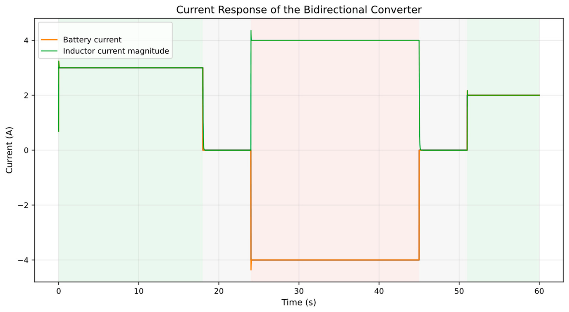
The simulated inductor current follows the magnitude of the imposed reference current during the active charging and discharging intervals. During the first charging interval, the converter increases the inductor current toward the prescribed positive-current level. After the transition to idle operation, the reference current becomes zero and the inductor current decreases accordingly. In the discharging interval, the reference-current sign changes, while the implemented current-control strategy regulates the inductor-current magnitude according to the absolute value of the reference. Finally, the converter returns to idle operation and then enters a second charging interval with a lower reference-current value.

The current response is shown in Figure 1. The figure compares the reference current and the simulated inductor current over the full operating sequence. In the reported numerical scenario, the current magnitude follows the imposed profile in both charging and discharging operation. Small deviations occur mainly during mode transitions because of the finite inductor response, duty-cycle saturation, and discrete-time PI action.

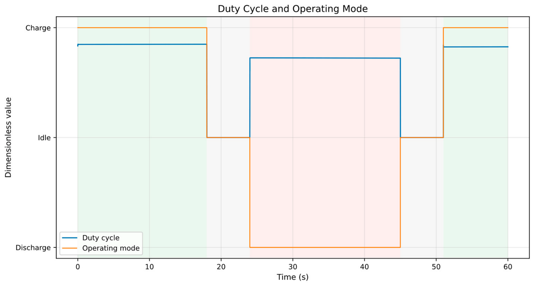
The operating-mode sequence and duty-cycle variation are shown in Figure 2. The mode signal matches the charging, idle, and discharging intervals selected from the reference-current sign and SOC constraints. During active power-transfer intervals, the duty cycle changes in response to the current-control error and the DC-link and battery-side voltages. During idle intervals, the converter does not intentionally transfer energy between the battery and the DC bus, and the control command is reduced accordingly.

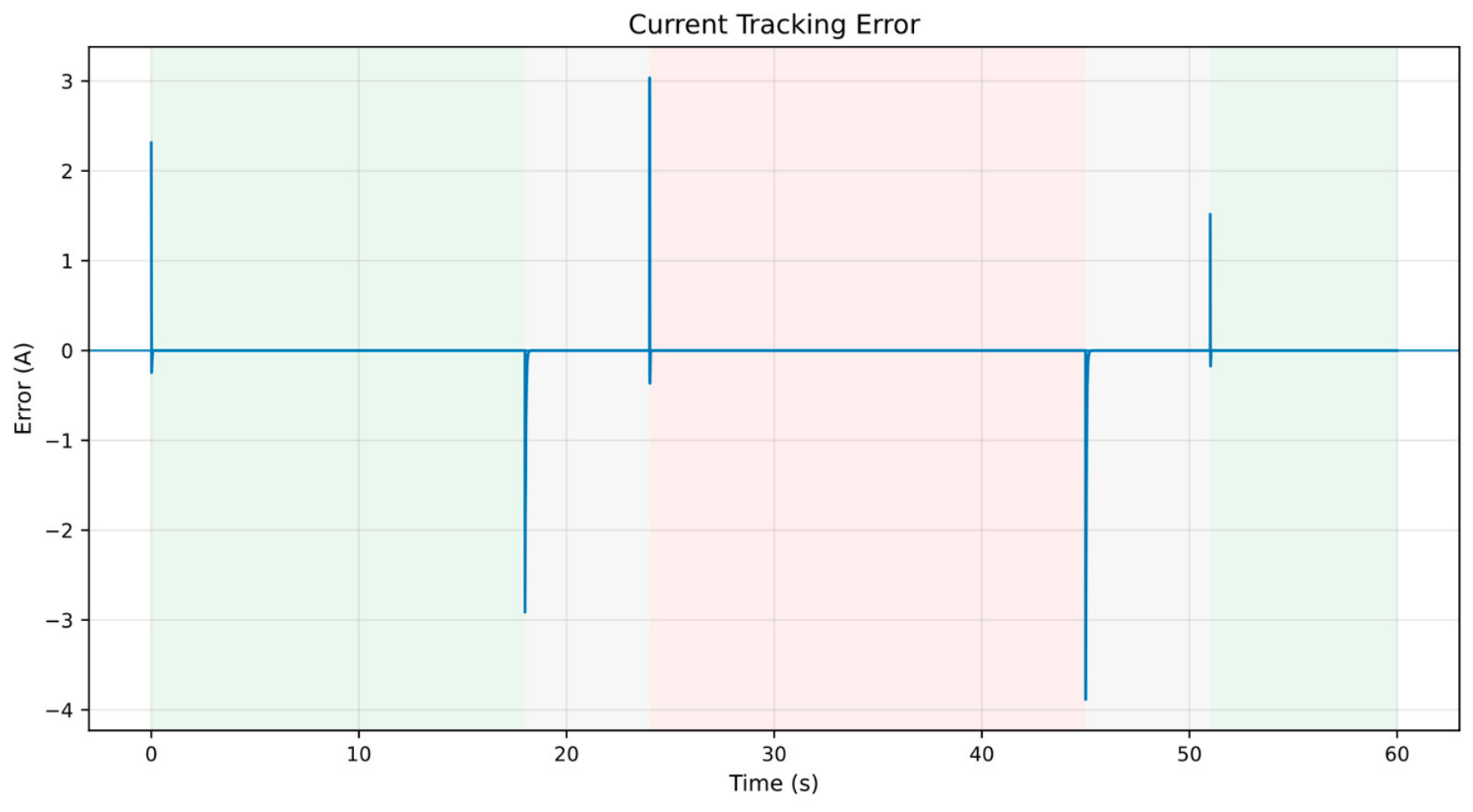
The current tracking error is shown in Figure 3. The error remains relatively small during the steady parts of the charging and discharging intervals and increases mainly at the instants of current-reference changes. These peaks are associated with the abrupt transition between different operating modes and reference-current levels. After each transition, the PI controller reduces the tracking error and drives the system toward the new operating condition.

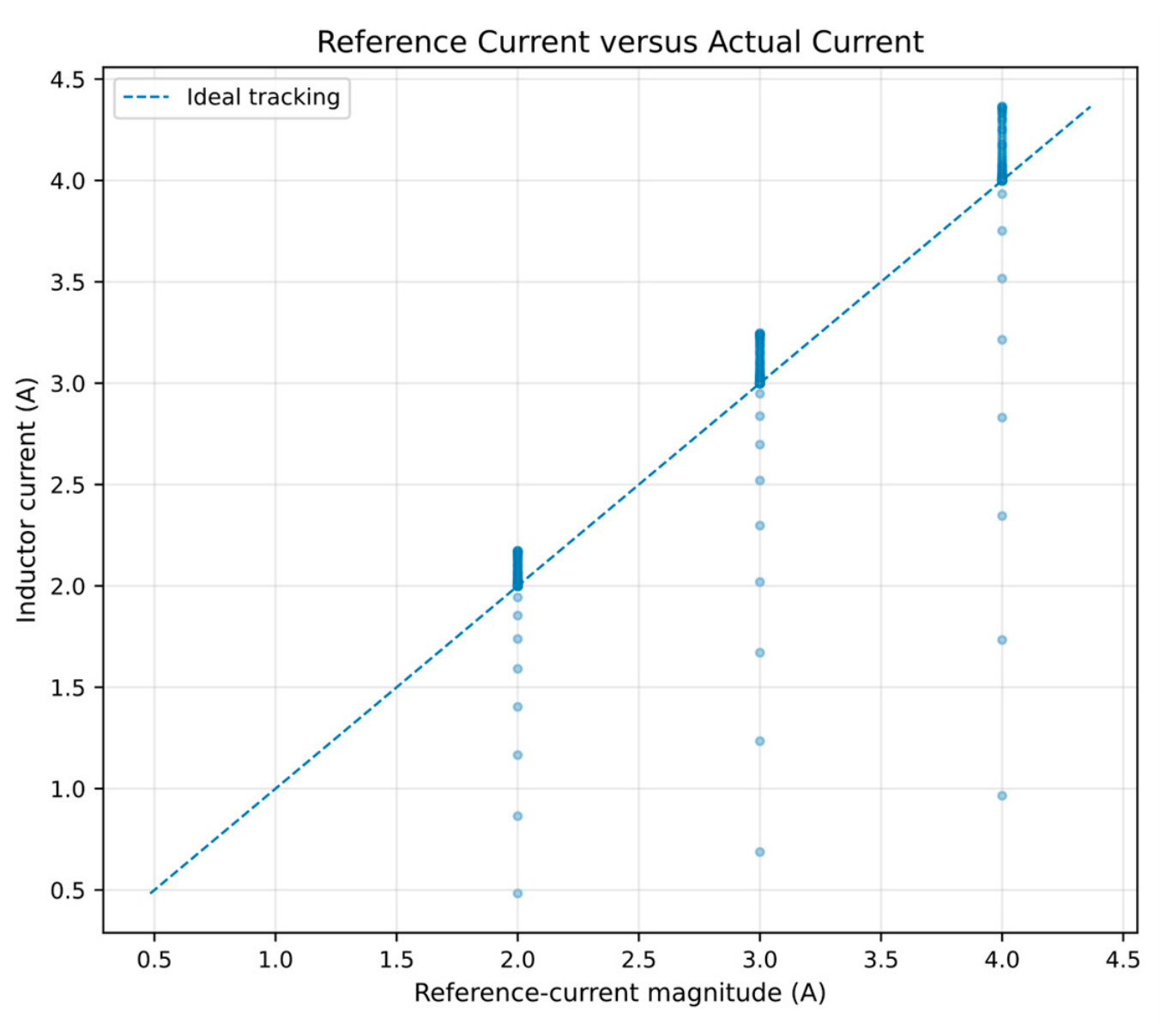
The relationship between the reference current and the simulated inductor current is further illustrated in Figure 4. This representation compares the commanded and obtained current values. The concentration of points near the ideal tracking line is consistent with bounded current-magnitude tracking within the tested numerical profile.

The results show that the implemented model reproduces the prescribed sequence and that the controller maintains bounded tracking in the tested profile. The largest errors occur at abrupt mode transitions, where the reference changes discontinuously and the duty cycle is constrained. These observations support use of the framework for numerical exploration of current regulation and mode transitions, but they do not constitute experimental validation.

5.3. Voltage-Related Diagnostics

The voltage diagnostics retained in this study are the battery polarization voltage and the DC-link voltage deviation. These quantities are reported separately to maintain a one-to-one correspondence between each figure and its discussion. A battery-terminal-voltage curve is not included; accordingly, no conclusion is drawn for that quantity.

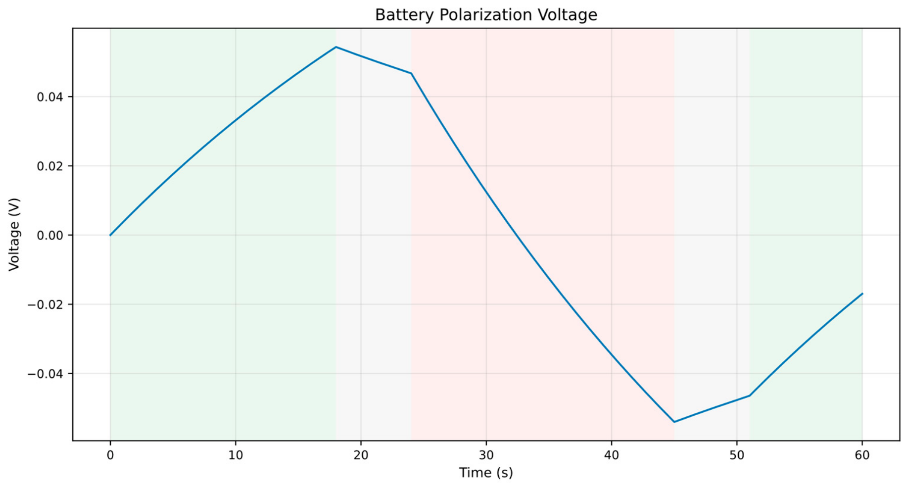
The polarization-voltage response is shown in Figure 5. It reflects the transient behavior of the Rp–Cp branch of the first-order Thevenin battery model. During charging and discharging, the polarization voltage changes with the battery-current direction and magnitude; during idle intervals, it relaxes according to the 40 s time constant.

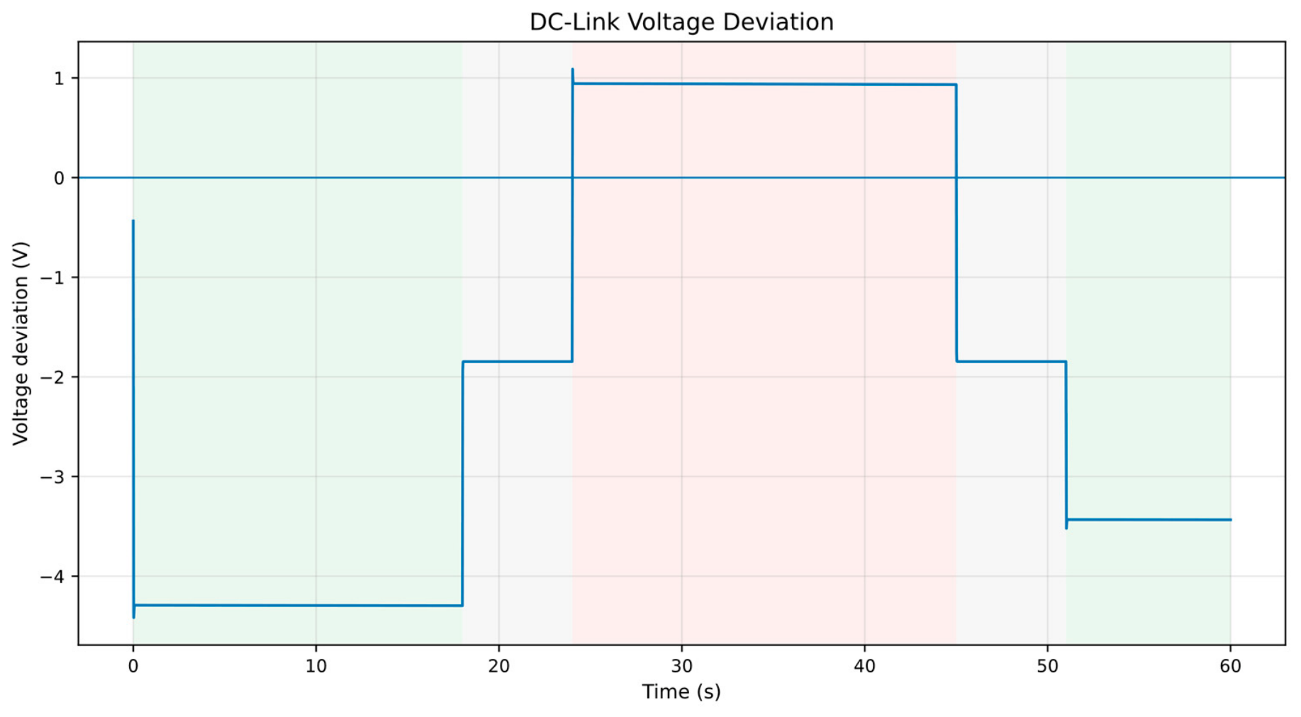
The DC-link voltage deviation is shown in Figure 6. The largest deviations occur around abrupt reference-current changes and active power-transfer intervals, whereas the deviation decreases during idle operation. The curve is a response of the adopted averaged numerical model and should not be interpreted as a measured voltage-regulation result.

Together, Figure 5 and Figure 6 show bounded voltage-related states over the reported 60 s scenario. The polarization branch exhibits the expected slow relaxation, while the DC-link deviation follows the changes in operating mode. Quantitative hardware conclusions require experimental parameters, step-size convergence, and measurement-based validation.

5.4. Battery SOC, Power Flow, and Energy Transfer

The battery state of charge, power-flow direction, and cumulative energy are analyzed to illustrate the bidirectional energy exchange represented by the numerical model, including charging, discharging, idle operation, and reversal of power flow.

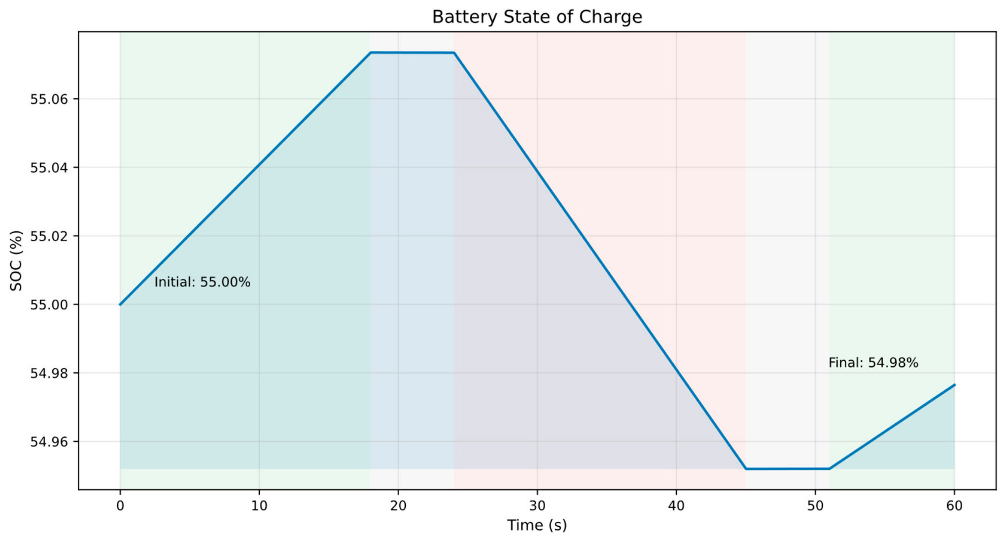
The physically scaled battery SOC is shown in Figure 7. It increases during charging, decreases during discharging, and remains nearly constant during idle operation, consistent with the sign convention and Coulomb-counting equation.

The SOC curve in Figure 7 uses KSOC = 1. Its sub-percentage variation over 60 s is compatible with the stated 20 Ah capacity and the short charge/discharge intervals.

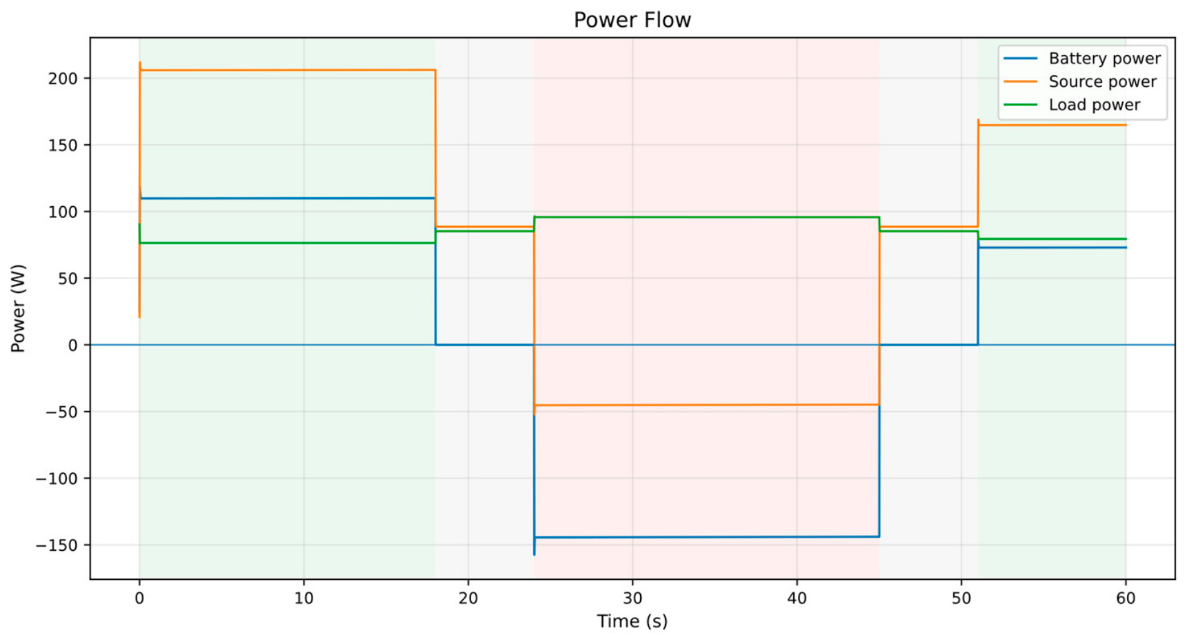
The instantaneous power-flow behavior is shown in Figure 8. Positive battery power denotes charging and negative battery power denotes discharging under the adopted sign convention. The first and final charging intervals therefore appear positive, while the −4 A interval produces negative battery power.

The idle intervals are characterized by a marked reduction in battery power, consistent with the supervisory logic reducing active power transfer when the reference current is zero. Small residual values may occur because of numerical dynamics, state relaxation, or controller and battery-model transients.

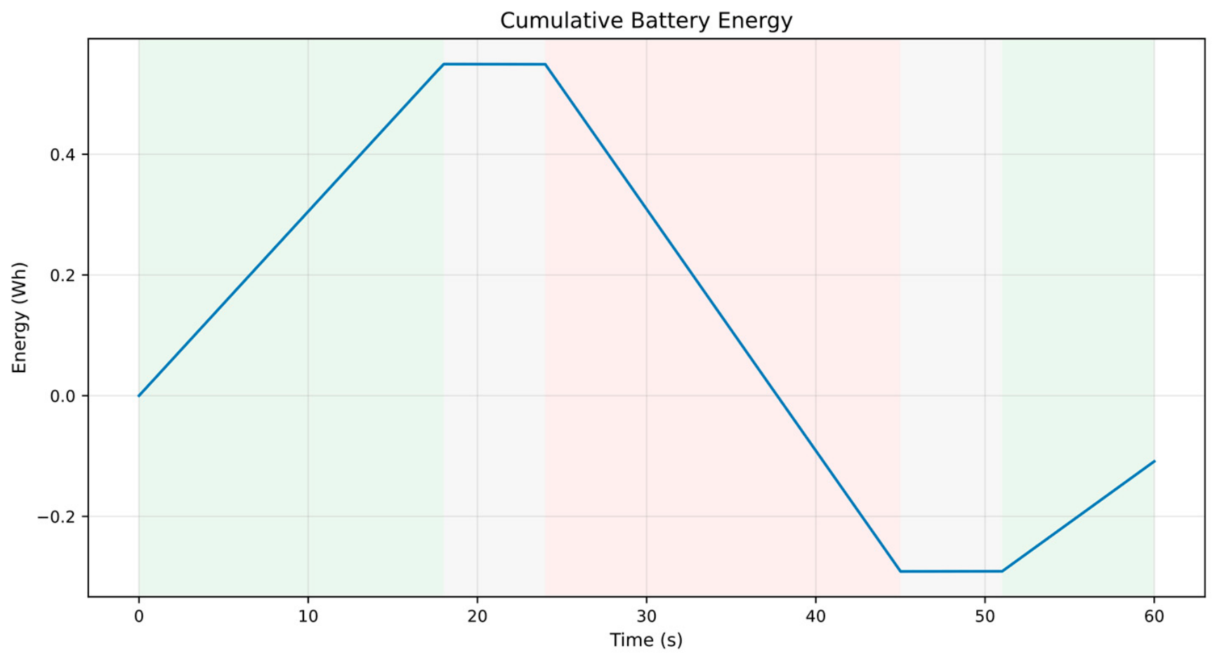
The cumulative battery energy is presented in Figure 9. Its slope follows the instantaneous battery power: it rises during charging, decreases during discharging, and changes only slightly in idle intervals. The larger discharge-current magnitude produces the largest energy change over the profile.

The energy-transfer results are consistent with the imposed current-reference sequence and selected operating modes. The converter first stores energy in the battery, pauses active exchange during idle operation, returns energy from the battery to the DC side during discharge, and finally enters a lower-power charging condition. This behavior is consistent with the intended bidirectional sign convention and operating sequence of the numerical model.

Overall, the SOC, power-flow, and cumulative-energy results show how the index matrix framework can be used, within the adopted model assumptions, to analyze energy exchange in bidirectional DC–DC converters. The model provides a clear distinction between charging and discharging operation, preserves the expected sign convention of battery power, and enables energy-transfer quantities to be evaluated together with current, voltage, and control responses.

5.5. Controller Performance and Error Metrics

The PI-controller results are quantified using error metrics rather than by repeating the current-error and reference-versus-actual plots already reported as Figure 3 and Figure 4. The error magnitude and its distribution are retained because they provide complementary information about transient peaks and the fraction of samples concentrated near zero.

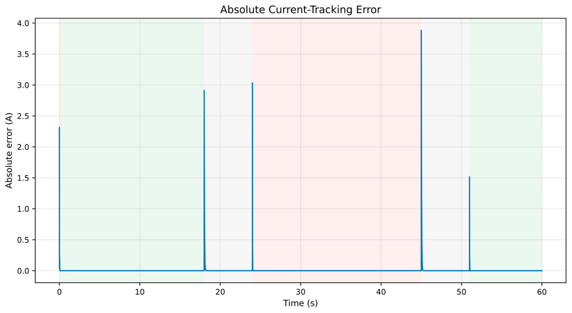
The absolute current error is presented in Figure 10. The largest values occur around mode transitions; after each transition, the error decreases as the numerical controller approaches the new operating condition.

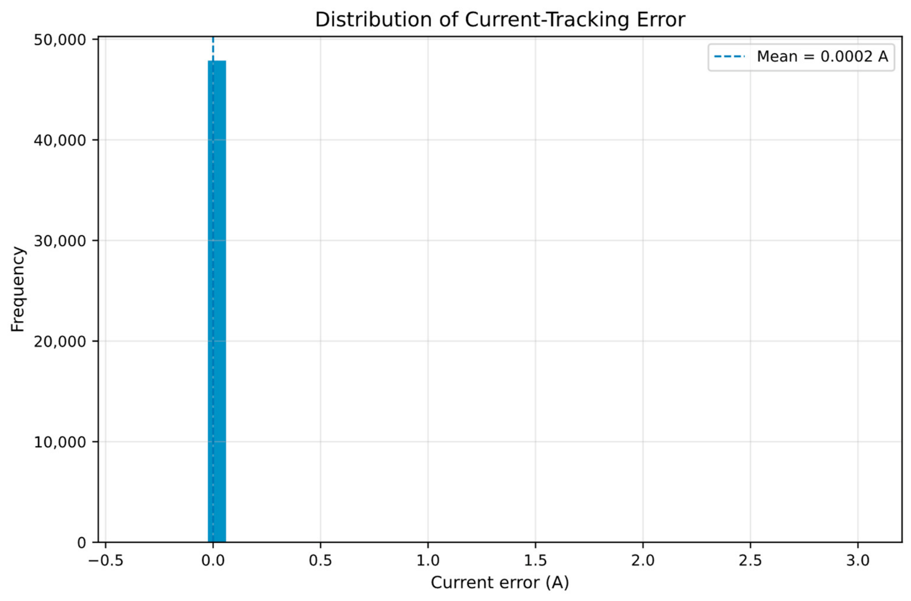
The distribution of the signed current error is illustrated in Figure 11. A concentration close to zero indicates that most samples belong to steady or near-steady intervals, whereas the tails correspond primarily to the short transition periods. The legend reports the signed sample mean (approximately 0.0002 A), whereas

Table 2. Current-tracking and full-profile dynamic indicators obtained from the simulation.

Metric	Symbol	Value	Unit
Root-mean-square current error	${\mathrm{RMSE}}_i$	0.0863	A
Mean absolute current error	${\mathrm{MAE}}_i$	0.0045	A
Integral absolute error	$\mathrm{IAE}$	0.2714	A·s
Integral squared error	$\mathrm{ISE}$	0.4472	A2·s
Integral time-weighted absolute error	$\mathrm{ITAE}$	8.6686	A·s2
Peak inductor current	$i_{L,\max }$	4.3684	A
Current overshoot	$M_{p,i}$	0.3684	A
Current overshoot	$M_{p,i,\%}$	9.2094	%
Last tolerance-band re-entry time (full profile)	$t_s$	51.0240	s
Full-profile inductor-current range	$\Delta i_{L,\mathrm{pp}}$	4.3684	A

reports the mean absolute error; these are distinct quantities. Sample-averaged metrics must therefore be interpreted together with RMSE and the peak error.

Table 2 summarizes RMSE, MAE, integral error measures, peak current, overshoot, the last tolerance-band re-entry time over the complete multi-step profile, and the full-profile current range. The last two quantities are not interpreted as the settling time or switching ripple of a single isolated step response.

The RMSE is 0.0863 A and the MAE is 0.0045 A. These values are internally consistent with the integral metrics over $T_{\mathrm{sim}}=60|\mathrm{s}$: $\mathrm{MAE}\approx \mathrm{IAE}/T_{\mathrm{sim}}=0.2714/60=0.00452|\mathrm{A}$ and $\mathrm{RMSE}\approx \sqrt{\mathrm{ISE}/T_{\mathrm{sim}}}=\sqrt{0.4472/60}=0.08633|\mathrm{A}$, with the small differences caused by rounding. IAE, ISE, and ITAE summarize one deterministic profile; they are not statistical confidence measures.

The peak inductor current is 4.3684 A, corresponding to 0.3684 A or 9.2094% above the maximum reference-current magnitude of 4 A. The event occurs at the idle-to-discharge transition, where the command changes abruptly from 0 to −4 A. Plausible contributors are the finite inductor dynamics, duty-cycle saturation, and the retained PI integral state at the mode transition; the available simulation does not isolate these mechanisms through a controller-state reset ablation.

The 9.2094% overshoot is reported as an outcome of the selected controller and step-reference profile and is not treated as universally acceptable. Hardware admissibility would have to be checked against semiconductor current ratings, inductor saturation, battery-current limits, protection thresholds, and thermal constraints.

If a smaller peak is required, appropriate remedies include a ramped current reference, bumpless transfer or integral-state reset at mode changes, revised anti-windup logic, explicit current limiting, and controller retuning. These alternatives are design recommendations and were not simulated in the present study.

The reported value of 51.0240 s is the last re-entry into the adopted tolerance band over a profile containing several steps and idle intervals. It is not the settling time of one isolated transition. Likewise, the 4.3684 A peak-to-peak value is the full-profile current range, not a switching-ripple measurement.

Overall, the metrics indicate small steady-interval tracking errors and short transition-dominated peaks for the selected scenario. The absence of repeated runs, parameter sweeps, or experimental data remains a limitation.

5.6. Conduction-Oriented Efficiency, Estimated Losses, and Energy Balance

This subsection reports internal energy accounting under the adopted simplified conduction-oriented loss model. The indicators complement the current, voltage, and SOC results but are not hardware-efficiency predictions.

The semiconductor switches are represented by algebraic conducting and blocking constraints, and the post-processing model mainly includes conduction-oriented terms. Switching-frequency-dependent turn-on and turn-off energy, diode reverse recovery, parasitic-capacitance loss, gate-drive power, magnetic core loss, temperature dependence, and thermal coupling are omitted. The efficiency values are therefore explicitly labeled as estimated conduction-oriented internal-model indicators.

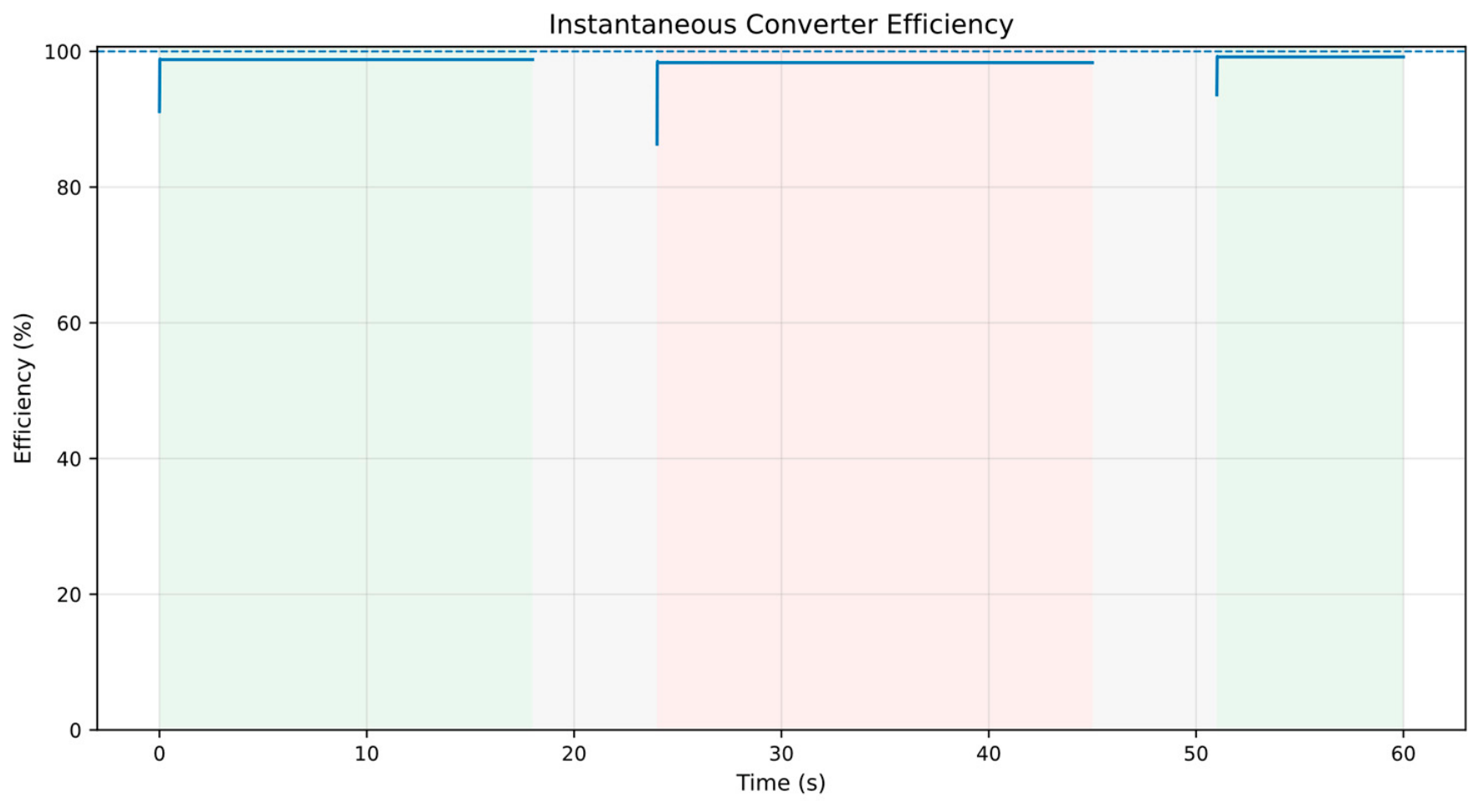
The estimated conduction-oriented instantaneous efficiency is shown in Figure 12 for active power-transfer intervals. Idle intervals are excluded from physical interpretation because the transferred power approaches zero and the ratio becomes ill-conditioned.

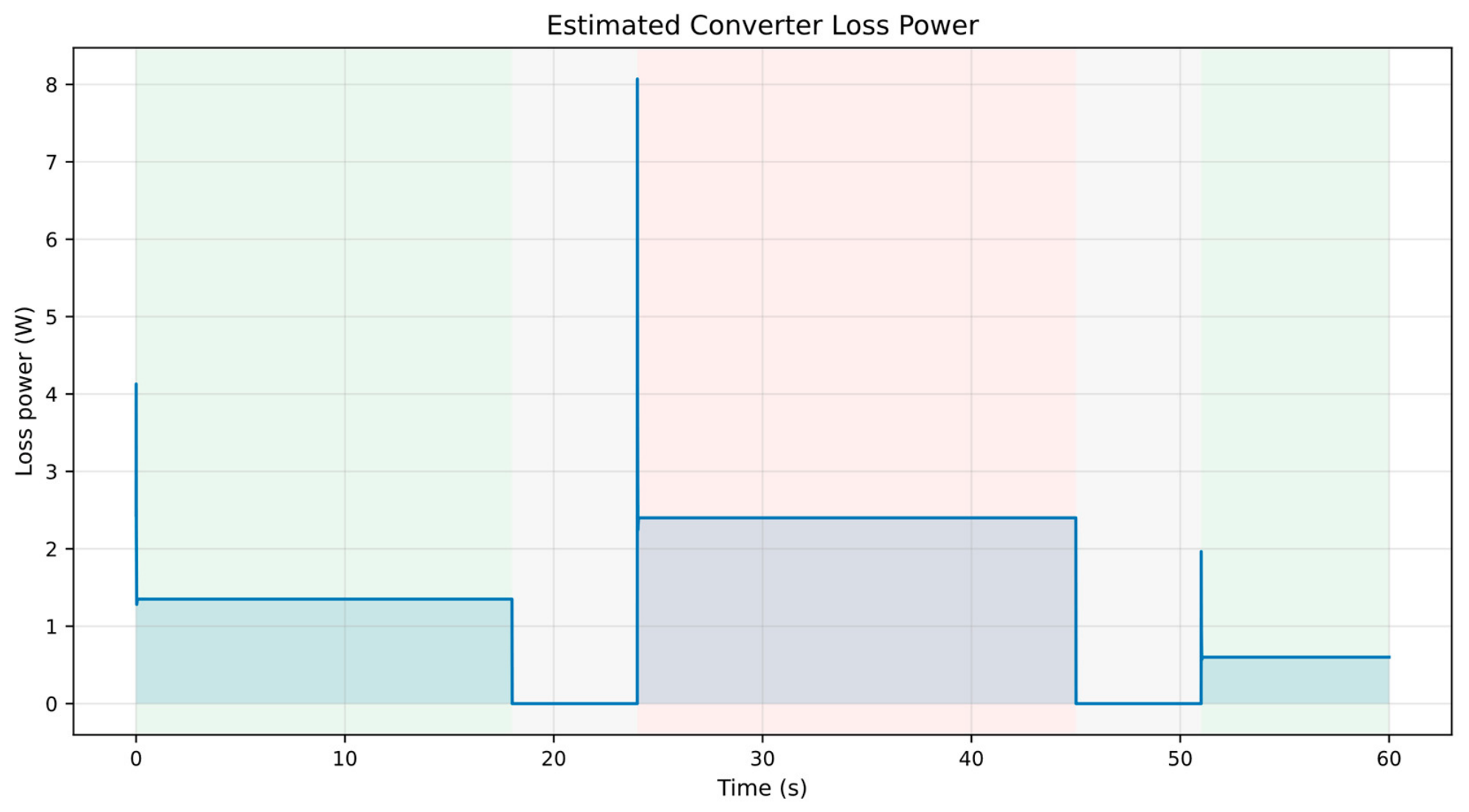
The estimated loss power is presented in Figure 13. It increases during active charging and discharging, with the largest values occurring at the higher current magnitude. The curve reflects the adopted post-processing equations only.

The energy quantities in

Table 3. Energy and loss indicators under the simplified conduction-oriented model.

Metric	Symbol	Value	Unit
Converter input energy	$E_{\mathrm{in}}$	1.6091	Wh
Converter output energy	$E_{\mathrm{out}}$	1.5868	Wh
Estimated converter loss energy	$E_{\mathrm{loss}}$	0.0223	Wh
Estimated conduction-oriented energy efficiency	${\eta }_E$	98.6166	%
Mean estimated conduction-oriented efficiency	$\stackrel{—}{\eta }$	98.6799	%
Peak converter loss power	$p_{\mathrm{loss},\max }$	7.9775	W
Charged battery energy	$E_{\mathrm{ch}}$	0.7488	Wh
Discharged battery energy	$E_{\mathrm{dis}}$	0.8521	Wh

are calculated independently by integrating the simulated power, so SOC represents accumulated charge, whereas the Wh values also include the time-varying battery voltage.

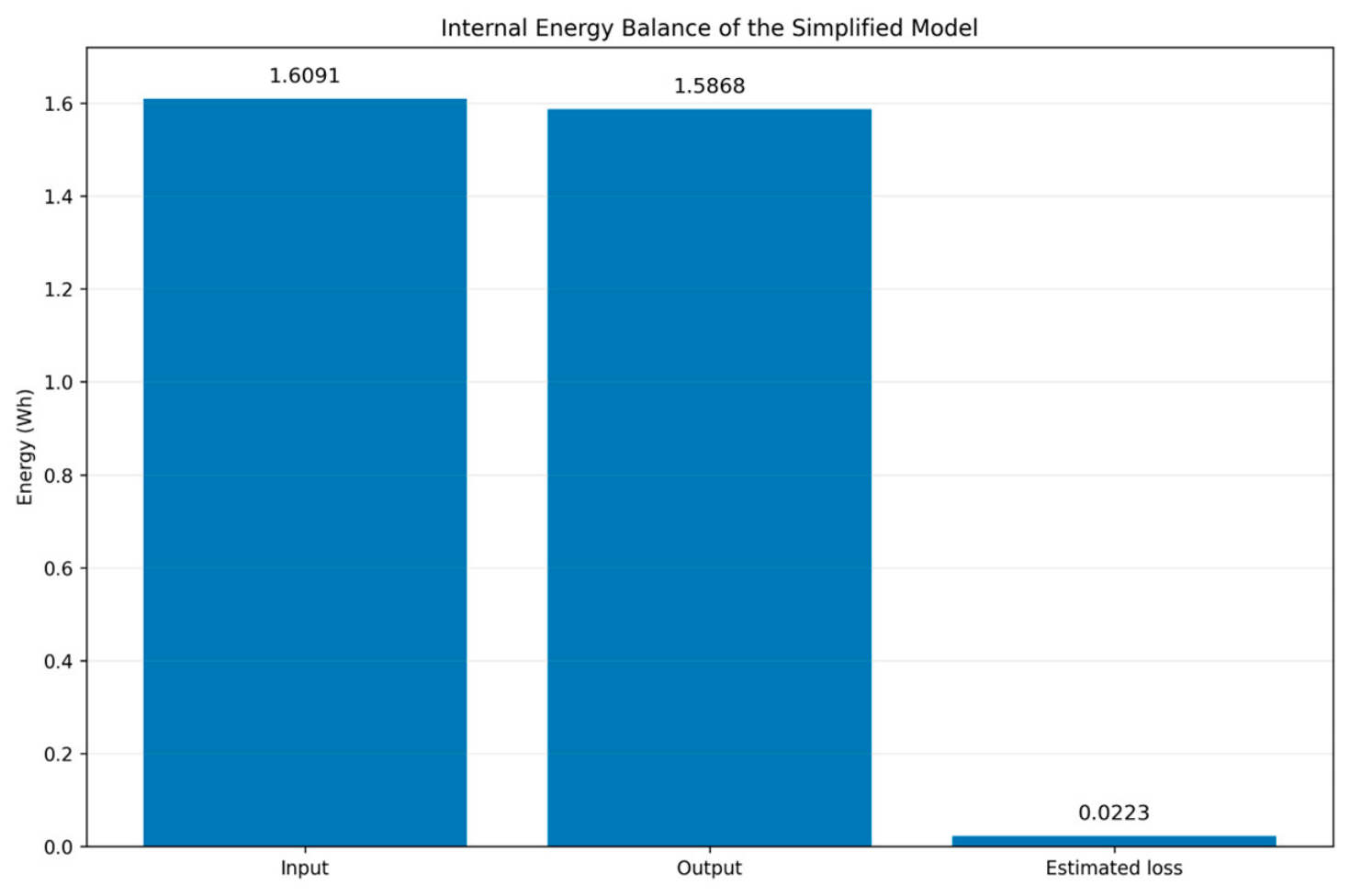
The integrated input energy is 1.6091 Wh, the output energy is 1.5868 Wh, and their difference is 0.0223 Wh. The corresponding estimated conduction-oriented internal-model efficiency is 98.6166%. This value is mathematically consistent with the stated energy balance, but it is not a hardware-efficiency prediction.

The mean estimated instantaneous efficiency is 98.6799%, close to the accumulated ratio. This agreement checks the internal post-processing arithmetic, not the completeness of the loss physics. Missing switching, magnetic, thermal, and auxiliary losses would reduce a hardware efficiency estimate.

The peak estimated loss power is 7.9775 W. Integrated battery energy is 0.7488 Wh during charging and 0.8521 Wh during discharging; the larger discharged value follows from the higher −4 A reference and interval durations. These quantities are obtained from power integration and are separate from the Coulomb-counted SOC calculation.

The internal energy balance is summarized in Figure 14. The correspondence E_in ≈ E_out + E_loss shows arithmetic closure for the adopted numerical model.

The interpretation is deliberately limited: the figures show internally consistent energy accounting under a conduction-oriented approximation. A realistic hardware-efficiency assessment would require a defined switching frequency, device switching-energy data or waveforms, magnetic-loss estimation, temperature-dependent parameters, auxiliary consumption, and experimental or detailed circuit-simulation benchmarking.

5.7. Local One-Step Sensitivity and Spectral-Radius Diagnostic

The finite-difference analysis is evaluated for representative charging, idle, and discharging operating points. It characterizes the immediate mapping of the four reported plant-and-battery states for a fixed operating mode and common pre-step controller memory. It is not a complete closed-loop state matrix because the PI integral memory is not included as an independent state.

For each mode, one state variable is perturbed at a time using the vector stated in Section 4.9, and the model is advanced by exactly one 1 ms step. The nominal and perturbed evaluations use the same mode and pre-step controller memory, while the duty command is recomputed from the corresponding state.

The resulting 4 × 4 matrix is therefore interpreted as a conditional one-step sensitivity matrix. Its eigenvalues may reveal numerical amplification or damping in the selected local mapping, but they cannot establish global or arbitrary-switching stability.

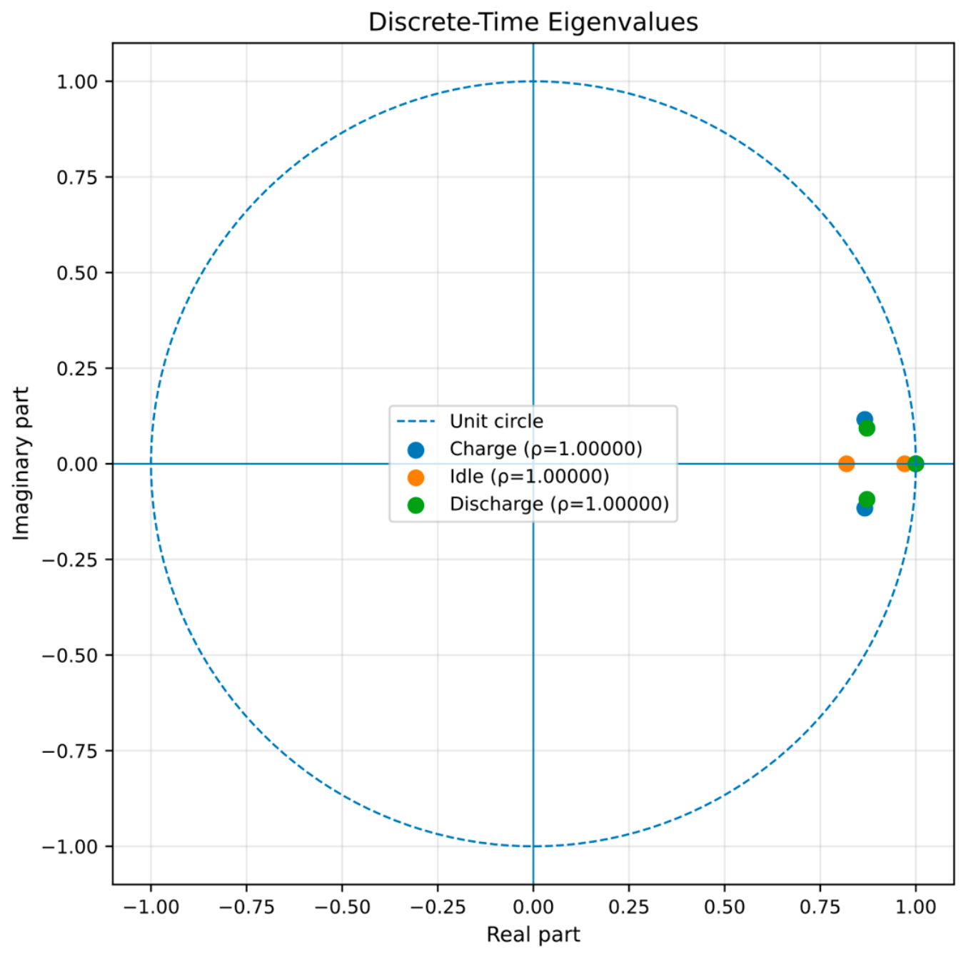
The eigenvalue locations are shown in Figure 15. Each mode contains one eigenvalue at z = 1, while the remaining electrical eigenvalues lie inside the unit circle for the selected operating points.

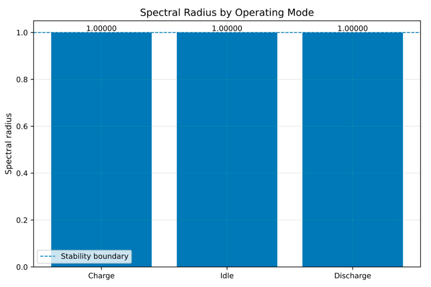
The corresponding spectral radii are shown in Figure 16. The plotted values are ρ = 1.00000 for charging, idle, and discharging; they are not below unity.

The unit spectral radius results from the eigenvalue at z = 1, which is consistent with the SOC-like integrating state over the one-step horizon. The full four-state mapping is therefore marginal or non-expansive at the displayed numerical precision, not locally asymptotically stable according to the strict criterion ρ < 1. The electrical eigenvalues inside the unit circle indicate local damping of the faster electrical components at the selected points.

The bounded 60 s trajectories are consistent with the absence of numerical divergence in the tested scenario, but bounded simulation alone is not a stability proof. In particular, no claim is made for controller-memory perturbations, other operating points, smaller time steps, parameter uncertainty, or arbitrary mode switching.

The eigenvalue analysis is retained as a transparent local diagnostic because it exposes both the damped electrical modes and the unit SOC mode. A formal closed-loop assessment would require augmenting the state with the PI integral memory, repeating the analysis over the operating domain, checking step-size sensitivity, and applying an appropriate switched-system or Lyapunov framework.

5.8. General Discussion

The study has several limitations that govern the interpretation of the results. First, it is a numerical modeling and software-level numerical-consistency study without experimental validation. Current, voltage, power, energy, and eigenvalue results are outputs of the adopted equations and parameter set rather than direct predictions of a laboratory converter.

Second, the semiconductor model contains simplified conducting and blocking constraints and a conduction-oriented post-processing loss estimate. Switching transients, reverse recovery, parasitic capacitances, gate-drive power, magnetic loss, temperature dependence, and thermal coupling are omitted; consequently, the reported efficiency values are estimated conduction-oriented internal-model indicators.

Third, the battery is represented by a first-order Thevenin equivalent circuit without detailed electrochemistry, temperature dependence, aging, hysteresis, or degradation. The reported results use $K_{\mathit{SOC}}=1$, so the displayed SOC is physically scaled; however, the parameters are illustrative rather than experimentally identified for a specific cell.

Fourth, the finite-difference matrix is local, one-step, fixed-mode, and conditional on common pre-step controller memory. The observed ρ = 1.00000 does not satisfy the strict asymptotic-stability condition and must not be reported as proof of local or switched-system stability.

Fifth, the study does not include a full parameter-sensitivity analysis, uncertainty analysis, step-size convergence test, experimental measurements, or a detailed circuit-simulation benchmark. These omissions limit quantitative hardware-oriented conclusions.

Within these limits, the label-aware index matrix framework provides a transparent way to assemble and simulate a multi-mode converter–battery–controller model in Python. Its principal value is methodological organization, traceable variable alignment, and reproducible generation of deterministic numerical outputs.

Future work should prioritize experimental validation, detailed semiconductor, magnetic, thermal, and auxiliary loss models, step-size convergence, parameter sensitivity and uncertainty, controller-state augmentation, comparison with a detailed switching-level benchmark, and formal analysis of the switched multi-mode system.

6. Conclusions

This paper presented a Python-based hybrid index matrix framework for label-aware assembly and simulation of a bidirectional buck–boost DC–DC converter connected to a first-order Thevenin battery model. Real-valued row and column identifiers preserve the relationship between component equations and physical variables before the system is projected into ordered numerical matrices for solution.

The workflow covers charging, idle, and discharging operation, supervisory mode selection, a discrete-time PI current controller with saturation and anti-windup, deterministic performance metrics, physically scaled SOC, conduction-oriented energy accounting, and a conditional one-step finite-difference diagnostic.

For the prescribed 60 s profile, the current RMSE is 0.0863 A and the peak current is 4.3684 A, corresponding to 9.2094% overshoot at the idle-to-discharge transition. The overshoot is reported as a scenario-dependent controller outcome; its hardware admissibility cannot be determined without current ratings, saturation limits, protection thresholds, and thermal constraints.

The SOC result uses $K_{\mathit{SOC}}=1$ and is therefore physically scaled according to the stated 20 Ah capacity and Coulomb-counting equation. Integrated power gives 0.7488 Wh charged energy and 0.8521 Wh discharged energy; these Wh quantities include the time-varying battery voltage and are not inferred directly from the SOC percentage.

The numerical energy balance is 1.6091 Wh input, 1.5868 Wh output, and 0.0223 Wh estimated loss. The corresponding 98.6166% ratio is an estimated conduction-oriented internal-model result and is not a hardware-efficiency prediction.

The conditional one-step matrices have spectral radius 1.00000 in all three fixed modes because of a unit SOC-related eigenvalue. The strict condition ρ < 1 is therefore not satisfied for the reported four-state mapping. The remaining electrical eigenvalues lie inside the unit circle, which supports only a local non-divergence interpretation for the selected points; it does not prove complete closed-loop or switched-system stability.

The main contribution is the transparent label-aware assembly of converter, battery, controller, and supervisory equations within one reproducible Python workflow. The reference ODE implementation serves only as a software-level numerical-consistency check between two formulations of the same assumptions.

The principal limitations are the absence of experimental validation; omission of detailed switching, magnetic, thermal, and auxiliary loss physics; lack of parameter-uncertainty and step-size-convergence studies; exclusion of controller memory from the eigenvalue state; and absence of formal switched-system analysis.

Future work will address laboratory validation, experimentally identified battery and semiconductor parameters, detailed switching, magnetic, thermal, and auxiliary loss models, smaller-step convergence tests, sensitivity and uncertainty analysis, improved transition control, comparison with specialized switching-level simulation, and augmented closed-loop stability analysis.