Several Structural Properties and Characterisations of Affine Gould–Hopper-Based Appell Polynomials

Abstract

In this paper, we introduce and systematically study a new two-parameter family of affine $(q,\eta )$-Gould–Hopper-based Appell polynomials. These polynomials arise by fusing the affine $(q,\eta )$-exponential Gould–Hopper kernel with an invertible Appell multiplier. A central contribution is the affine quasi-monomial construction: an explicit raising operator obtained from a logarithmic-difference quotient of the combined kernel, together with the lowering operator and the resulting q-commutation structure. An explicit double-sum series representation and an affine diffusion equation of order j connecting differences in the two variables, and the full quasi-monomial framework identifying the operator pair $(P_{q,\eta }^{+},P_{q,\eta }^{-})$ are developed. Additional results include a governing difference equation, a converse characterisation, a determinantal representation, an affine addition formula, and an order recursion. Further, the Bernoulli and Euler sub-families are obtained as invertible specialisations, while the Genocchi family is treated separately as a derived noninvertible family through its exact relation with the Euler family. The corresponding structural results are stated with these hypotheses made explicit. Surface plots, numerical value tables, and a numerical illustration of real zeros accompany the theoretical development. The diffusion relation provides a discrete affine analogue of a higher-order evolution equation; no claim of a fully developed physical model is made in the present work.

1. Introduction and Preliminaries

Special polynomials—including Hermite, Laguerre, Legendre, Jacobi, Bernoulli, Euler, Genocchi, Appell, and Sheffer families among them—form one of the most enduring pillars of mathematical analysis, arising independently in approximation theory, combinatorics, number theory, probability, quantum mechanics, and the spectral theory of differential operators. Their study is organised around tightly interlocking structural properties such as generating functions, differential or difference equations, Rodrigues-type formulas when available, and raising and lowering (ladder) operators. Orthogonality is a defining feature only for particular subclasses (and is not assumed for a general Appell, Bernoulli-, Euler-, or Genocchi-type sequence); more generally, algebraic characterisations can be formulated through the quasi-monomiality principle of Steffensen and Dattoli, which views the family as the orbit of a single “vacuum” element under iterated application of a multiplicative operator. The passage from one variable to several variables—and from the ordinary calculus to q-calculus, $(p,q)$-calculus, or affine $(q,\omega )$-calculus—has been a dominant theme in modern special-function theory, driven both by internal algebraic demands (umbral calculus, operad structures, Rota–Baxter algebras) and by applications in mathematical physics (multi-dimensional harmonic oscillators, lattice path enumeration, quantum groups, and discrete integrable systems). Multivariate special polynomials such as the Hermite–Kampé de Fériet polynomials in two variables, the Gould–Hopper polynomials $g_n^{\left(j\right)}(u,v)$ of arbitrary order j, the multivariate Laguerre and Jacobi families on simplices and balls, and the multivariable Appell and Sheffer systems extend many classical structural constructions—generating functions, differential or difference equations, ladder operators, determinantal representations, and addition theorems—to the richer geometric and algebraic setting furnished by several independent variables, while simultaneously introducing new phenomena such as higher-order diffusion equations linking the variables, multi-index recurrences, and intertwining relations among the partial-derivative or partial-difference operators acting in different directions. In this broader landscape, the construction of hybrid families—obtained by coupling a multivariate exponential or q-exponential kernel with an invertible Appell multiplier—has emerged as a particularly fruitful strategy, producing Bernoulli- and Euler-type extensions directly within the invertible Appell framework; related Genocchi-type families may also be obtained, subject to the appropriate normalisation or derived-family interpretation when the corresponding generator has vanishing constant term. These constructions connect the combinatorial content encoded in the Appell numbers with the analytic and physical content carried by the kernel. The Gould–Hopper polynomials $g_n^{\left[j\right]}(u,v)$ in two variables, introduced in [1], are generated by

$$e^{u\mu +v{\mu }^j}=\sum _{n\ge 0}{g}_n^{\left[j\right]}(u,v){\displaystyle \frac{{\mu }^n}{n!}},j\ge 2.$$

(1)

They extend the classical Hermite polynomials (recovered at $j=2$, $v=-\frac{1}{2}$ after rescaling) and reduce to the elementary monomials at $v=0$. Their operational structure—the j-th order diffusion relation ${\partial }_v{g}_n^{\left[j\right]}={\partial }_u^j{g}_n^{\left[j\right]}$, ladder operators, determinantal representations, and addition identities—serves as a model for quasi-monomial and umbral constructions [1,2]. Appell-type deformations, formed by multiplying the exponential by an invertible series $\mathcal{A}\left(\mu \right)$, extend this model directly to Bernoulli- and Euler-type two-variable families; related Genocchi-type families can be incorporated through an appropriate derived-family or normalised-shift interpretation [3,4,5].

The affine $(q,\eta )$-calculus is built on the shift $u\mapsto qu+\eta$ with $0<q<1$ and $0<\eta <1$ in the non-degenerate affine case. Throughout the analytical theory, we use this range; the boundary value $\eta =0$ is also admitted as the standard limiting q-difference case and is used explicitly in the numerical illustrations below, as formulated by Annaby, Hamza and Aldwoah [6] in the context of the Hahn difference operator. It replaces $e^{u\mu }$ by the affine exponential ${\mathcal{E}}_{q,\eta }(u,\mu )$ of [7]. Ernst [8] provides the comprehensive q-calculus background. The $(q,\eta )$-Appell polynomial framework was developed in [7,9], and Hahn–Appell polynomials with their d-orthogonality were studied by Varma, Yaşar and Özarslan [10]. Recent developments in closely related q-deformed and hybrid polynomial systems include degenerate q-derangement numbers and polynomials [11], lacunary bivariate q-Laguerre polynomials of Sheffer type with applications to heterogeneous graph filters [12], and a degenerate q-hybrid Heine equation together with Beta-kernel integral representations [13]. Further related contributions concern two-variable q-Gould–Hopper–Hahn Appell polynomials [14], and q-truncated exponential-based Hahn Appell polynomials [15]. These studies further illustrate the continuing role of Appell–Sheffer structures, q-calculus, and hybrid generating kernels in the construction and characterisation of generalised special-polynomial families.

The present paper fuses the Appell framework with the bivariate Gould–Hopper kernel ${\mathcal{E}}_{q,\eta }(v,{\mu }^j)$ for a general integer $j\ge 2$, producing the affine $(q,\eta )$-Gould–Hopper–Appell family; the precise generating equation is given as Definition 1 in Section 2.

The monomiality principle, developed by Dattoli [4] on foundations of Steffensen [2], characterises a polynomial family through a raising operator $P_{q,\eta }^{+}$ and a lowering operator $P_{q,\eta }^{-}$ satisfying $P_{q,\eta }^{+}{p}_n=p_{n+1}$ and $P_{q,\eta }^{-}{p}_n={⟨n⟩}_q{p}_{n-1}$. Ben Cheikh [16] showed how dual sequences arise from this principle. Özarslan and Yılmaz [17] obtained finite-order differential equations for Appell polynomials; Sharma and Chak [18] and Sadjang [19] developed basic and $(p,q)$-analogues. Bivariate degenerate Appell families were studied in [3,20], and further relevant results appear in [21,22].

Comparison with Earlier Work

The present construction differs from the cited classical, q-, $(p,q)$-, and degenerate Appell frameworks in three linked respects. The affine Hahn shift $u\mapsto qu+\eta$ is retained simultaneously in both variables; the Gould–Hopper factor introduces an arbitrary diffusion order $j\ge 2$ rather than only the ordinary Hermite case; and the combined kernel is used to derive a single quasi-monomial raising operator, q-commutation relation, determinantal representation, addition formula, and affine diffusion relation for the whole class. Thus, the novelty is not merely a new list of special polynomials, but the unified operator framework connecting the affine Appell multiplier with the bivariate Gould–Hopper kernel. The Bernoulli and Euler examples are genuine invertible specialisations of this general class, whereas the Genocchi case requires the separate normalisation explained in Section 4 because its generator has zero constant term.

We fix notation throughout, following [6,7]. Set ${\eta }_0:=\eta /(1-q)$. The q-number and q-factorial are

$${⟨k⟩}_q:={\displaystyle \frac{1-q^k}{1-q}},{⟨k⟩}_q!:={\displaystyle \prod _{m=1}^k}{⟨m⟩}_q,{⟨0⟩}_q!:=1.$$

(2)

The affine $(q,\eta )$-difference operator [6,7] is

$${\Delta }_{q,\eta }\left(\phi \right)\left(u\right):=\left\{\begin{array}{cc}{\displaystyle \frac{\phi (qu+\eta )-\phi \left(u\right)}{(q-1)u+\eta }},\hfill & u\ne {\eta }_0,\hfill \\ {\phi }^{\prime }\left(u\right),\hfill & u={\eta }_0,\hfill \end{array}\right.$$

(3)

with Leibniz rule ([7], Equation (6))

$${\Delta }_{q,\eta ,u}\left(fg\right)\left(u\right)=f(qu+\eta ){\Delta }_{q,\eta ,u}g\left(u\right)+g\left(u\right){\Delta }_{q,\eta ,u}f\left(u\right).$$

(4)

The affine factorial sequences ([7], Equations (7) and (8)) are

$${\left(u\right)}_{q,\eta }^k:={\displaystyle \prod _{m=0}^{k-1}}(u-\eta {⟨m⟩}_q),{\left[u\right]}_{q,\eta }^k:={\displaystyle \prod _{m=0}^{k-1}}(q^{m}u+\eta {⟨m⟩}_q),$$

(5)

satisfying ${\Delta }_{q,\eta }{\left(u\right)}_{q,\eta }^n={⟨n⟩}_q{\left(u\right)}_{q,\eta }^{n-1}$ ([7], Equation (9)). The affine $(q,\eta )$-exponential ([7], Equation (14)) is

$${\mathcal{E}}_{q,\eta }(u,\mu ):=\sum _{k\ge 0}{\left(u\right)}_{q,\eta }^k{\displaystyle \frac{{\mu }^k}{{⟨k⟩}_q!}},$$

(6)

the unique solution of ${\Delta }_{q,\eta ,u}f=\mu f$, $f\left(0\right)=1$ ([7], Theorem 1.6). The q-binomial coefficient is

$${\left[\begin{array}{c}n\\ k\end{array}\right]}_q:={\displaystyle \frac{{⟨n⟩}_q!}{{⟨k⟩}_q!{⟨n-k⟩}_q!}}.$$

(7)

The Newton–Ward–Appell (NWA) $q,\eta$-addition ([7], Equation (21)) is

$${\left(u{\oplus }_{q,\eta }w\right)}^n:={\displaystyle \sum _{k=0}^n}{\left[\begin{array}{c}n\\ k\end{array}\right]}_q{\left(u\right)}_{q,\eta }^{n-k}{\left(w\right)}_{q,\eta }^k,$$

(8)

with exponential addition formula ([7], Corollary 2.2)

$${\mathcal{E}}_{q,\eta }(u{\oplus }_{q,\eta }w,\mu )={\mathcal{E}}_{q,\eta }(u,\mu ){\mathcal{E}}_{q,\eta }(w,\mu ).$$

The affine exponential satisfies

$${\Delta }_{q,\eta ,u}{\mathcal{E}}_{q,\eta }(u,\mu )=\mu {\mathcal{E}}_{q,\eta }(u,\mu ).$$

(9)

For differentiation with respect to the generating parameter, we use the Jackson q-derivative

$$D_{q,\mu }F\left(\mu \right):={\displaystyle \frac{F\left(\mu \right)-F\left(q\mu \right)}{(1-q)\mu }}.$$

From (6) and ${\left(u\right)}_{q,\eta }^{m+1}=(u-\eta {⟨m⟩}_q){\left(u\right)}_{q,\eta }^m$, one obtains

$$D_{q,\mu }{\mathcal{E}}_{q,\eta }(u,\mu )={\displaystyle \frac{u}{1+\eta \mu }}{\mathcal{E}}_{q,\eta }(u,\mu ).$$

(10)

This distinction is essential when $\eta \ne 0$; at $\eta =0$, it reduces to the usual Jackson identity. An order-n multiplicative Appell generator ([7], Equation (44)) is $f^n(\mu ,q,\eta )=h{(\mu ,q,\eta )}^n={\sum }_{\ell \ge 0}{\mathrm{\Phi }}_{\ell ,q,\eta }^{\left(n\right)}{\mu }^{\ell }/{⟨\ell ⟩}_q!$, with ${\mathrm{\Phi }}_{0,q,\eta }^{\left(n\right)}=1$.

Three principal contributions are made. First, the complete quasi-monomial framework for the affine $(q,\eta )$-Gould–Hopper–Appell polynomials ${}_{\mathcal{G}}\mathcal{A}_{n;q,\eta }^{\left[j\right]}(u,v)$ is established. Second, the affine j-th order diffusion equation ${\Delta }_{q,\eta ,v}{}_{\mathcal{G}}\mathcal{A}_{n;q,\eta }^{\left[j\right]}={\Delta }_{q,\eta ,u}^j{}_{\mathcal{G}}\mathcal{A}_{n;q,\eta }^{\left[j\right]}$ is proved for every admissible multiplier $\mathcal{A}$ and every admissible $\eta$, including the boundary specialisation $\eta =0$ where indicated. Third, the Bernoulli, Euler, and Genocchi specialisations yield the Gould–Hopper–Bernoulli, –Euler, and –Genocchi polynomial families with explicit generating functions, the structural results valid under the appropriate invertibility hypotheses, surface plots, numerical tables, and a numerical zero study.

Section 2 introduces the generating function, the series representation, and establishes the lowering operator, the affine diffusion equation, and the raising operator for the general family. Section 3 continues the structural theory with the commutation relations, the full quasi-monomial characterisation, the governing difference equation, the converse and determinantal representations, the affine addition formula, and the order recursion, all accompanied by surface plots and a numerical table. Section 4 presents three distinguished examples—the Hermite-based Bernoulli, Euler, and Genocchi polynomial families—with explicit generating functions, series representations, polynomial tables, surface plots, and a numerical investigation of the real-zero distribution for selected parameter values. Section 5 gives conclusions and discusses several promising avenues for future investigation.

2. Affine $(\mathit{q},\mathit{\eta })$-Gould–Hopper–Appell Polynomials

The affine $(q,\eta )$-Gould–Hopper–Appell polynomials introduced in this section represent a natural multi-parameter deformation of the classical bivariate Gould–Hopper–Appell family, obtained by replacing the ordinary exponential kernel with its affine analogue ${\mathcal{E}}_{q,\eta }(u,\mu ){\mathcal{E}}_{q,\eta }(v,{\mu }^j)$ and coupling it to a general invertible Appell multiplier $\mathcal{A}(\mu ,q,\eta )$ in the sense of [7,9]. The parameter $q\in (0,1)$ controls the degree of quantum deformation, with $q\to 1$ recovering the classical theory, while $\eta \in (0,1)$ introduces the affine shift $u\mapsto qu+\eta$ into every factorial and exponential factor [6,8]. The integer $j\ge 2$ controls the order of the diffusion-like kernel; $j=2$ recovers the Hermite (Kampé de Fériet) case.

Definition 1 ($(q,\eta )$-Gould–Hopper–Appell generating function).

Let

$$\mathcal{A}(\mu ,q,\eta )=\sum _{k\ge 0}{\mathcal{A}}_{k;q,\eta }{\displaystyle \frac{{\mu }^k}{{⟨k⟩}_q!}},{\mathcal{A}}_{0;q,\eta }:=1,$$

(11)

be an invertible Appell multiplier. The affine $(q,\eta )$-Gould–Hopper–Appell polynomials of order j ${\{{}_{\mathcal{G}}\mathcal{A}_{n;q,\eta }^{\left[j\right]}(u,v)\}}_{n\ge 0}$ are defined by

$$\mathcal{A}(\mu ,q,\eta ){\mathcal{E}}_{q,\eta }(u,\mu ){\mathcal{E}}_{q,\eta }(v,{\mu }^j)={\displaystyle \sum _{n=0}^{\infty }}{}_{\mathcal{G}}\mathcal{A}_{n;q,\eta }^{\left[j\right]}(u,v){\displaystyle \frac{{\mu }^n}{{⟨n⟩}_q!}}.$$

(12)

Here, ${\mathcal{E}}_{q,\eta }(v,{\mu }^j)={\sum }_{\ell \ge 0}{\left(v\right)}_{q,\eta }^{\ell }{\mu }^{j\ell }/{⟨\ell ⟩}_q!$ is the $(q,\eta )$-Gould–Hopper kernel of order j, with j-th-multiple-index coefficients ${⟨j\ell ⟩}_q!{\left(v\right)}_{q,\eta }^{\ell }/{⟨\ell ⟩}_q!$ and vanishing non-multiple-of-j coefficients.

Theorem 1 (Series representation).

For every $n\ge 0$,

$${}_{\mathcal{G}}\mathcal{A}_{n;q,\eta }^{\left[j\right]}(u,v)={\displaystyle \sum _{k=0}^n}{\displaystyle \sum _{\ell =0}^{\lfloor k/j\rfloor }}{\left[\begin{array}{c}n\\ k\end{array}\right]}_q{\left[\begin{array}{c}k\\ j\ell \end{array}\right]}_q{\left(u\right)}_{q,\eta }^{n-k}{\mathcal{A}}_{k-j\ell ;q,\eta }{\displaystyle \frac{{⟨j\ell ⟩}_q!}{{⟨\ell ⟩}_q!}}{\left(v\right)}_{q,\eta }^{\ell }.$$

(13)

Proof. 

We begin by introducing the combined Appell–Gould–Hopper kernel

$${\mathcal{K}}_{q,\eta }^{\left[j\right]}(v,\mu ):=\mathcal{A}(\mu ,q,\eta ){\mathcal{E}}_{q,\eta }(v,{\mu }^j),$$

and write its expansion as ${\mathcal{K}}_{q,\eta }^{\left[j\right]}(v,\mu )={\sum }_{k\ge 0}{\mathrm{\Xi }}_{k;q,\eta }\left(v\right){\mu }^k/{⟨k⟩}_q!$. To determine ${\mathrm{\Xi }}_{k;q,\eta }\left(v\right)$, we form the Cauchy product of

$$\mathcal{A}(\mu ,q,\eta )=\sum _{r\ge 0}{\mathcal{A}}_{r;q,\eta }{\displaystyle \frac{{\mu }^r}{{⟨r⟩}_q!}}\mathrm{and}{\mathcal{E}}_{q,\eta }(v,{\mu }^j)=\sum _{\ell \ge 0}{\left(v\right)}_{q,\eta }^{\ell }{\displaystyle \frac{{\mu }^{j\ell }}{{⟨\ell ⟩}_q!}}.$$

Writing ${\varphi }_{i;q,\eta }\left(v\right)$ for the coefficient of ${\mu }^i/{⟨i⟩}_q!$ in ${\mathcal{E}}_{q,\eta }(v,{\mu }^j)$, we observe that this exponential contains only j-th power multiples of $\mu$, so

$${\varphi }_{i;q,\eta }\left(v\right)=\left\{\begin{array}{cc}{\displaystyle \frac{{⟨j\ell ⟩}_q!}{{⟨\ell ⟩}_q!}}{\left(v\right)}_{q,\eta }^{\ell },\hfill & \mathrm{if}i=j\ell \mathrm{for}\mathrm{some}\ell \in {\mathbb{Z}}_{\ge 0},\hfill \\ 0,\hfill & \mathrm{if}j\nmid i.\hfill \end{array}\right.$$

The Cauchy product with the q-Vandermonde convolution then gives

$${\mathrm{\Xi }}_{k;q,\eta }\left(v\right)={\displaystyle \sum _{i=0}^k}{\left[\begin{array}{c}k\\ i\end{array}\right]}_q{\mathcal{A}}_{k-i;q,\eta }{\varphi }_{i;q,\eta }\left(v\right).$$

Since ${\varphi }_{i;q,\eta }=0$ whenever $j\nmid i$, the only surviving terms are those with $i=j\ell$ for $\ell =0,1,\dots ,\lfloor k/j\rfloor$. Substituting $i=j\ell$ yields

$${\mathrm{\Xi }}_{k;q,\eta }\left(v\right)={\displaystyle \sum _{\ell =0}^{\lfloor k/j\rfloor }}{\left[\begin{array}{c}k\\ j\ell \end{array}\right]}_q{\mathcal{A}}_{k-j\ell ;q,\eta }{\displaystyle \frac{{⟨j\ell ⟩}_q!}{{⟨\ell ⟩}_q!}}{\left(v\right)}_{q,\eta }^{\ell }.$$

(14)

A second Cauchy product between ${\mathcal{K}}_{q,\eta }^{\left[j\right]}(v,\mu )$ and ${\mathcal{E}}_{q,\eta }(u,\mu )={\sum }_{m\ge 0}{\left(u\right)}_{q,\eta }^m{\mu }^m/{⟨m⟩}_q!$, extracting the coefficient of ${\mu }^n/{⟨n⟩}_q!$, gives

$${}_{\mathcal{G}}\mathcal{A}_{n;q,\eta }^{\left[j\right]}(u,v)={\displaystyle \sum _{k=0}^n}{\left[\begin{array}{c}n\\ k\end{array}\right]}_q{\left(u\right)}_{q,\eta }^{n-k}{\mathrm{\Xi }}_{k;q,\eta }\left(v\right).$$

Substituting (14) yields (13). □

Corollary 1 (Pure $(q,\eta )$-Gould–Hopper polynomials).

Setting ${\mathcal{A}}_{0;q,\eta }=1$ and ${\mathcal{A}}_{k;q,\eta }=0$ for $k\ge 1$,

$$G_{n;q,\eta }^{\left[j\right]}(u,v)={\displaystyle \sum _{\ell =0}^{\lfloor n/j\rfloor }}{\left[\begin{array}{c}n\\ j\ell \end{array}\right]}_q{\left(u\right)}_{q,\eta }^{n-j\ell }{\displaystyle \frac{{⟨j\ell ⟩}_q!}{{⟨\ell ⟩}_q!}}{\left(v\right)}_{q,\eta }^{\ell },$$

(15)

which as $(q,\eta )\to (1,0)$ tends to $g_n^{\left[j\right]}(u,v)=n!{\sum }_{\ell }{u}^{n-j\ell }{v}^{\ell }/((n-j\ell )!\ell !)$, the classical Gould–Hopper polynomial. At $j=2$, this recovers the Kampé de Fériet–Hermite polynomial.

• Numerical table. Table 1 records values of the general polynomial ${}_{\mathcal{G}}\mathcal{A}_{n;1/2,0}^{\left[j\right]}(u,v)$ computed via (13) with the Bernoulli multiplier at $q=\frac{1}{2}$, $\eta =0$, $j=2$; the entries confirm that the generating equation (12) is consistent across six orders and eight sample points.
  Table 1. Values of ${}_{\mathcal{G}}\mathcal{A}_{n;1/2,0}^{\left[2\right]}(u,v)$ (Bernoulli multiplier, $q=\frac{1}{2}$, $\eta =0$) for $n=0,\dots ,5$.

  u	v	$\mathit{n}=0$	$\mathit{n}=1$	$\mathit{n}=2$	$\mathit{n}=3$	$\mathit{n}=4$	$\mathit{n}=5$
  0.5	0.0	1	−0.1667	−0.1548	−0.0611	−0.0171	−0.0034
  1.0	0.0	1	0.3333	0.0952	0.0222	0.0037	0.0002
  2.0	0.0	1	1.3333	2.0952	3.6889	6.9204	13.4084
  0.5	0.5	1	−0.1667	0.5952	−0.2799	0.5493	−0.3793
  1.0	0.5	1	0.3333	0.8452	0.4597	0.9803	0.5703
  2.0	0.5	1	1.3333	2.8452	5.4389	11.1782	22.2281
  1.0	1.0	1	0.3333	1.5952	0.8972	3.5975	2.2000
  2.0	1.0	1	1.3333	3.5952	7.1889	17.0766	35.2860

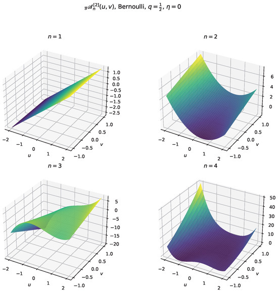
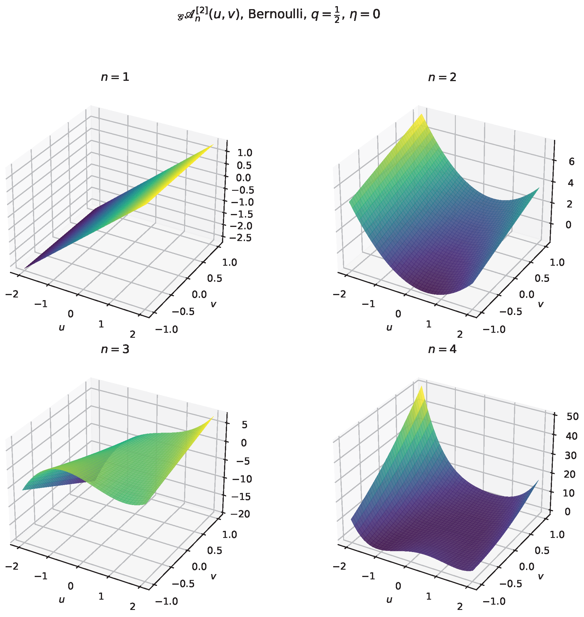
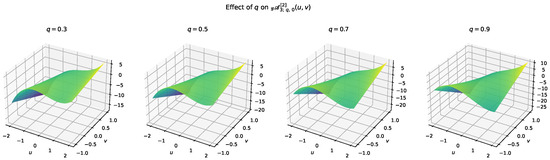
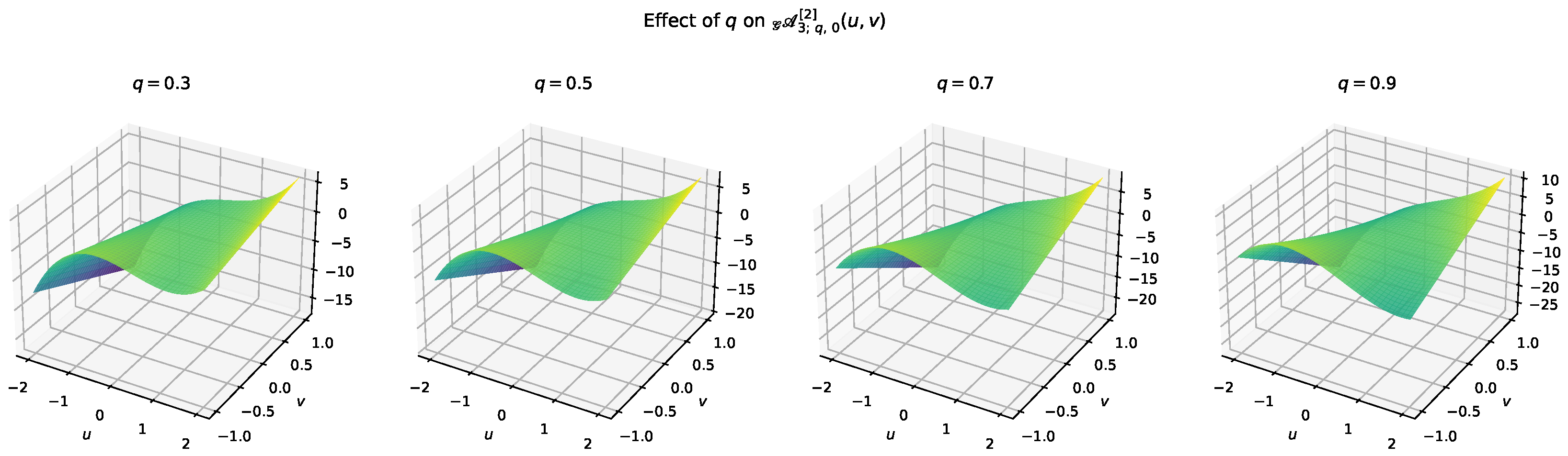
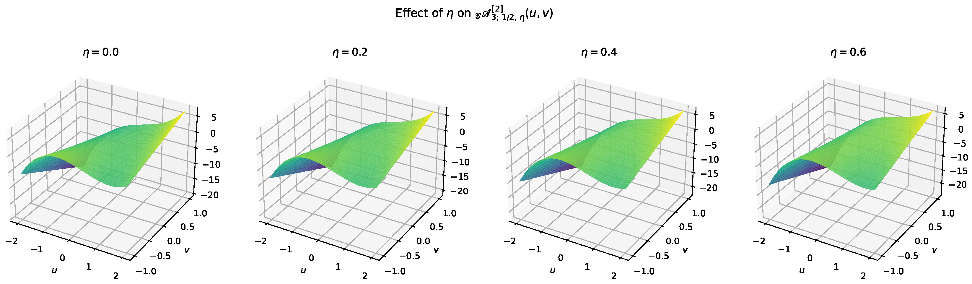
Figure 1, Figure 2 and Figure 3 illustrate the surface of ${}_{\mathcal{G}}\mathcal{A}_{n;q,\eta }^{\left[j\right]}(u,v)$ as computed by (13), revealing how the degree and the deformation parameters jointly govern the shape of the polynomial surface.

Figure 1. Surfaces of ${}_{\mathcal{G}}\mathcal{A}_{n;1/2,0}^{\left[2\right]}(u,v)$ (Definition 1, Bernoulli multiplier) for $n=1,2,3,4$ over $[-2,2]\times [-1,1]$ at $q=\frac{1}{2}$, $\eta =0$.

Figure 2. Effect of q on ${}_{\mathcal{G}}\mathcal{A}_{3;q,0}^{\left[2\right]}(u,v)$ for $q\in \{0.3,0.5,0.7,0.9\}$, $\eta =0$.

Figure 3. Effect of $\eta$ on ${}_{\mathcal{G}}\mathcal{A}_{3;1/2,\eta }^{\left[2\right]}(u,v)$ for $\eta \in \{0,0.2,0.4,0.6\}$, $q=\frac{1}{2}$.

Theorem 2 (Lowering operator $P_{q,\eta }^{-}$).

$P_{q,\eta }^{-}:={\Delta }_{q,\eta ,u}$ satisfies

$$P_{q,\eta }^{-}{}_{\mathcal{G}}\mathcal{A}_{n;q,\eta }^{\left[j\right]}(u,v)={⟨n⟩}_q{}_{\mathcal{G}}\mathcal{A}_{n-1;q,\eta }^{\left[j\right]}(u,v),n\ge 1,P_{q,\eta }^{-}{}_{\mathcal{G}}\mathcal{A}_{0;q,\eta }^{\left[j\right]}=0.$$

(16)

Proof. 

We apply ${\Delta }_{q,\eta ,u}$ to both sides of (12). On the right-hand side,

$${\Delta }_{q,\eta ,u}{\displaystyle \sum _{n=0}^{\infty }}{}_{\mathcal{G}}\mathcal{A}_{n;q,\eta }^{\left[j\right]}(u,v){\displaystyle \frac{{\mu }^n}{{⟨n⟩}_q!}}={\displaystyle \sum _{n=1}^{\infty }}{\Delta }_{q,\eta ,u}\left[{}_{\mathcal{G}}\mathcal{A}_{n;q,\eta }^{\left[j\right]}\right]{\displaystyle \frac{{\mu }^n}{{⟨n⟩}_q!}},$$

where the $n=0$ term vanishes since ${}_{\mathcal{G}}\mathcal{A}_{0;q,\eta }^{\left[j\right]}={\mathcal{A}}_{0;q,\eta }=1$ is constant in u. On the left-hand side, the combined kernel ${\mathcal{K}}_{q,\eta }^{\left[j\right]}(v,\mu )$ is independent of u, so by the Leibniz rule (4), ${\Delta }_{q,\eta ,u}\left[{\mathcal{K}}_{q,\eta }^{\left[j\right]}(v,\mu ){\mathcal{E}}_{q,\eta }(u,\mu )\right]={\mathcal{K}}_{q,\eta }^{\left[j\right]}(v,\mu )·\mu {\mathcal{E}}_{q,\eta }(u,\mu )$ by (9). Re-expanding and equating coefficients of ${\mu }^n/{⟨n⟩}_q!$ gives ${\Delta }_{q,\eta ,u}{}_{\mathcal{G}}\mathcal{A}_{n;q,\eta }^{\left[j\right]}={⟨n⟩}_q{}_{\mathcal{G}}\mathcal{A}_{n-1;q,\eta }^{\left[j\right]}$. □

Theorem 3 (Affine $(q,\eta )$-diffusion equation of order j).

For every $\mathcal{A}$ and every $n\ge 0$,

$${\Delta }_{q,\eta ,v}{}_{\mathcal{G}}\mathcal{A}_{n;q,\eta }^{\left[j\right]}(u,v)={\Delta }_{q,\eta ,u}^j{}_{\mathcal{G}}\mathcal{A}_{n;q,\eta }^{\left[j\right]}(u,v),$$

(17)

or equivalently for $n\ge j$, ${\Delta }_{q,\eta ,v}{}_{\mathcal{G}}\mathcal{A}_{n;q,\eta }^{\left[j\right]}={\prod }_{i=0}^{j-1}{⟨n-i⟩}_q{}_{\mathcal{G}}\mathcal{A}_{n-j;q,\eta }^{\left[j\right]}$.

Proof. 

Step 1. From ${\Delta }_{q,\eta ,v}{\mathcal{E}}_{q,\eta }(v,s)=s{\mathcal{E}}_{q,\eta }(v,s)$ (shown as in the Hermite case), setting $s={\mu }^j$ gives ${\Delta }_{q,\eta ,v}{\mathcal{E}}_{q,\eta }(v,{\mu }^j)={\mu }^j{\mathcal{E}}_{q,\eta }(v,{\mu }^j)$.

Step 2. Since $\mathcal{A}(\mu ,q,\eta )$ and ${\mathcal{E}}_{q,\eta }(u,\mu )$ are independent of v, ${\Delta }_{q,\eta ,v}\left[\mathcal{A}·{\mathcal{E}}_{q,\eta }(u,\mu )·{\mathcal{E}}_{q,\eta }(v,{\mu }^j)\right]={\mu }^j·\mathcal{A}·{\mathcal{E}}_{q,\eta }(u,\mu )·{\mathcal{E}}_{q,\eta }(v,{\mu }^j)$. Applying ${\Delta }_{q,\eta ,u}^j$ to the same product and using (9) j times multiplies by ${\mu }^j$, giving the same result.

Step 3. Comparing coefficients of ${\mu }^n/{⟨n⟩}_q!$ yields (17). For $n\ge j$, j successive applications of Theorem 2 give the explicit falling-factorial form. □

Theorem 4 (Raising operator $P_{q,\eta }^{+}$).

Write ${\mathcal{K}}_{q,\eta }^{\left[j\right]}(v,\mu ):=\mathcal{A}(\mu ,q,\eta ){\mathcal{E}}_{q,\eta }(v,{\mu }^j)$. The operator

$$P_{q,\eta }^{+}:={\left[{\displaystyle \frac{D_{q,\tau }{\mathcal{K}}_{q,\eta }^{\left[j\right]}(v,\tau )}{{\mathcal{K}}_{q,\eta }^{\left[j\right]}(v,\tau )}}+{\displaystyle \frac{u{\mathcal{K}}_{q,\eta }^{\left[j\right]}(v,q\tau )}{(1+\eta \tau ){\mathcal{K}}_{q,\eta }^{\left[j\right]}(v,\tau )}}\right]}_{\tau ={\Delta }_{q,\eta ,u}}$$

(18)

satisfies $P_{q,\eta }^{+}{}_{\mathcal{G}}\mathcal{A}_{n;q,\eta }^{\left[j\right]}={}_{\mathcal{G}}\mathcal{A}_{n+1;q,\eta }^{\left[j\right]}$.

Proof. 

Apply the Jackson derivative $D_{q,\mu }$ to (12). Using $D_{q,\mu }\left(FG\right)=G\left(\mu \right)D_{q,\mu }F\left(\mu \right)+F\left(q\mu \right)D_{q,\mu }G\left(\mu \right)$ and (10), the left-hand side equals

$$\left[{\displaystyle \frac{D_{q,\mu }\mathcal{K}(v,\mu )}{\mathcal{K}(v,\mu )}}+{\displaystyle \frac{u\mathcal{K}(v,q\mu )}{(1+\eta \mu )\mathcal{K}(v,\mu )}}\right]\mathcal{K}(v,\mu ){\mathcal{E}}_{q,\eta }(u,\mu ),$$

where $\mathcal{K}={\mathcal{K}}_{q,\eta }^{\left[j\right]}$. The right-hand side becomes ${\sum }_{n\ge 0}{}_{\mathcal{G}}\mathcal{A}_{n+1;q,\eta }^{\left[j\right]}{\mu }^n/{⟨n⟩}_q!$. The substitution $\tau ={\Delta }_{q,\eta ,u}$ is understood in the formal-power-series sense. Since $\mathcal{K}(v,0)=1$ and $1+\eta \tau$ has nonzero constant term, all required reciprocals exist uniquely. On a polynomial of degree n in u, ${\Delta }_{q,\eta ,u}^r=0$ for $r>n$, so the substituted series truncate. Hence, no additional analytic convergence assumption is needed. Comparing coefficients proves the result. □

3. Algebraic Characteristics

Together, these results furnish a complete algebraic toolkit that will be specialised directly to the Bernoulli and Euler sub-families in Section 4. The Genocchi-derived family is treated separately through its exact relation with the Euler family, since its generating multiplier has vanishing constant term and is therefore noninvertible.

Theorem 5 (q-commutation relations).

With $P_{q,\eta }^{-}={\Delta }_{q,\eta ,u}$ and $P_{q,\eta }^{+}$ from (18), one has

$$\left(P_{q,\eta }^{-}{P}_{q,\eta }^{+}-q{P}_{q,\eta }^{+}{P}_{q,\eta }^{-}\right){}_{\mathcal{G}}\mathcal{A}_{n;q,\eta }^{\left[j\right]}(u,v)={}_{\mathcal{G}}\mathcal{A}_{n;q,\eta }^{\left[j\right]}(u,v).$$

(19)

More generally, for every integer $m\ge 1$,

$$\left(P_{q,\eta }^{-}{\left(P_{q,\eta }^{+}\right)}^m-q^m{\left(P_{q,\eta }^{+}\right)}^m{P}_{q,\eta }^{-}\right){}_{\mathcal{G}}\mathcal{A}_{n;q,\eta }^{\left[j\right]}(u,v)={⟨m⟩}_q{}_{\mathcal{G}}\mathcal{A}_{n+m-1;q,\eta }^{\left[j\right]}(u,v).$$

(20)

Consequently, the ordinary commutator satisfies

$$[P_{q,\eta }^{-},P_{q,\eta }^{+}]{}_{\mathcal{G}}\mathcal{A}_{n;q,\eta }^{\left[j\right]}(u,v)=q^n{}_{\mathcal{G}}\mathcal{A}_{n;q,\eta }^{\left[j\right]}(u,v).$$

(21)

Proof. 

The result follows directly from the raising and lowering relations, together with

$${⟨n+1⟩}_q-q{⟨n⟩}_q=1$$

and, more generally,

$${⟨n+m⟩}_q-q^m{⟨n⟩}_q={⟨m⟩}_q.$$

For the ordinary commutator, using $P_{q,\eta }^{-}{P}_{q,\eta }^{+}-q{P}_{q,\eta }^{+}{P}_{q,\eta }^{-}=I$ gives

$$[P_{q,\eta }^{-},P_{q,\eta }^{+}]=I+(q-1)P_{q,\eta }^{+}{P}_{q,\eta }^{-}.$$

Since

$$P_{q,\eta }^{+}{P}_{q,\eta }^{-}{}_{\mathcal{G}}\mathcal{A}_{n;q,\eta }^{\left[j\right]}={⟨n⟩}_q{}_{\mathcal{G}}\mathcal{A}_{n;q,\eta }^{\left[j\right]},$$

we obtain

$$[P_{q,\eta }^{-},P_{q,\eta }^{+}]{}_{\mathcal{G}}\mathcal{A}_{n;q,\eta }^{\left[j\right]}=\left(1+(q-1){⟨n⟩}_q\right){}_{\mathcal{G}}\mathcal{A}_{n;q,\eta }^{\left[j\right]}=q^n{}_{\mathcal{G}}\mathcal{A}_{n;q,\eta }^{\left[j\right]}.$$

□

• $\mathit{q}$-quasi-monomiality principle. We use the natural q-analogue: fixed operators $M,P$ satisfy $M{p}_n=p_{n+1}$, $P{p}_n={⟨n⟩}_q{p}_{n-1}$, $PM-qMP=I$, and $p_n=M^n\left\{1\right\}$. This reduces to the classical monomiality principle as $q\to 1$.

Theorem 6 (q-quasi-monomial characterisation).

The family

$${\left\{{}_{\mathcal{G}}\mathcal{A}_{n;q,\eta }^{\left[j\right]}(u,v)\right\}}_{n\ge 0}$$

is q-quasi-monomial under the fixed operator pair $P_{q,\eta }^{+}$ defined in (18) and $P_{q,\eta }^{-}:={\Delta }_{q,\eta ,u}$. More precisely,

$$\begin{array}{cc}\hfill P_{q,\eta }^{+}{}_{\mathcal{G}}\mathcal{A}_{n;q,\eta }^{\left[j\right]}(u,v)& ={}_{\mathcal{G}}\mathcal{A}_{n+1;q,\eta }^{\left[j\right]}(u,v),\hfill \end{array}$$

(22)

$$\begin{array}{cc}\hfill P_{q,\eta }^{-}{}_{\mathcal{G}}\mathcal{A}_{n;q,\eta }^{\left[j\right]}(u,v)& ={⟨n⟩}_q{}_{\mathcal{G}}\mathcal{A}_{n-1;q,\eta }^{\left[j\right]}(u,v),\hfill \end{array}$$

(23)

and

$$P_{q,\eta }^{-}{P}_{q,\eta }^{+}-q{P}_{q,\eta }^{+}{P}_{q,\eta }^{-}=I$$

(24)

on the polynomial family. Furthermore,

$${}_{\mathcal{G}}\mathcal{A}_{n;q,\eta }^{\left[j\right]}(u,v)={\left(P_{q,\eta }^{+}\right)}^n\left\{1\right\},$$

(25)

and the associated number-operator relation is

$$P_{q,\eta }^{+}{P}_{q,\eta }^{-}{}_{\mathcal{G}}\mathcal{A}_{n;q,\eta }^{\left[j\right]}(u,v)={⟨n⟩}_q{}_{\mathcal{G}}\mathcal{A}_{n;q,\eta }^{\left[j\right]}(u,v).$$

(26)

As $(q,\eta )\to (1,0)$,

$$P_{q,\eta }^{-}⟶{\partial }_u,P_{q,\eta }^{+}⟶u+jv{\partial }_u^{j-1}+{\displaystyle \frac{{\mathcal{A}}^{\prime }\left({\partial }_u\right)}{\mathcal{A}\left({\partial }_u\right)}},$$

so the classical Gould–Hopper–Appell monomiality structure is recovered.

Proof. 

The raising and lowering relations follow from Theorem 2 and Theorem 4, respectively, while the q-commutation relation follows from Theorem 5. Since

$${}_{\mathcal{G}}\mathcal{A}_{0;q,\eta }^{\left[j\right]}(u,v)=1,$$

successive applications of $P_{q,\eta }^{+}$ yield

$${}_{\mathcal{G}}\mathcal{A}_{n;q,\eta }^{\left[j\right]}(u,v)={\left(P_{q,\eta }^{+}\right)}^n\left\{1\right\}.$$

The number-operator identity follows by first applying $P_{q,\eta }^{-}$ and then $P_{q,\eta }^{+}$. Finally, the classical limit follows from $D_{q,\tau }\to {\partial }_{\tau }$, $\mathcal{K}(v,q\tau )\to \mathcal{K}(v,\tau )$, ${\Delta }_{q,\eta ,u}\to {\partial }_u$, and $\eta \to 0$. □

Theorem 7 (Governing difference equation).

For each $n\ge 0$,

$$\left(P_{q,\eta }^{+}{\Delta }_{q,\eta ,u}-{⟨n⟩}_q\right){}_{\mathcal{G}}\mathcal{A}_{n;q,\eta }^{\left[j\right]}=0,$$

with $P_{q,\eta }^{+}$ given explicitly by (18).

Proof. 

By the lowering relation,

$$P_{q,\eta }^{-}{}_{\mathcal{G}}\mathcal{A}_{n;q,\eta }^{\left[j\right]}={⟨n⟩}_q{}_{\mathcal{G}}\mathcal{A}_{n-1;q,\eta }^{\left[j\right]}.$$

Applying $P_{q,\eta }^{+}$ and using the raising relation gives

$$P_{q,\eta }^{+}{P}_{q,\eta }^{-}{}_{\mathcal{G}}\mathcal{A}_{n;q,\eta }^{\left[j\right]}={⟨n⟩}_q{}_{\mathcal{G}}\mathcal{A}_{n;q,\eta }^{\left[j\right]}.$$

Since $P_{q,\eta }^{-}={\Delta }_{q,\eta ,u}$, this is precisely the stated governing difference equation. □

Theorem 8 (Converse representation).

If ${\Delta }_{q,\eta ,u}{P}_{n;q,\eta }={⟨n⟩}_q{P}_{n-1;q,\eta }$ and ${\Delta }_{q,\eta ,u}{P}_0=0$, then unique ${\mathrm{\Xi }}_{k;q,\eta }\left(v\right)$ exist with

$$P_{n;q,\eta }(u,v)={\displaystyle \sum _{k=0}^n}{\left[\begin{array}{c}n\\ k\end{array}\right]}_q{\left(u\right)}_{q,\eta }^{n-k}{\mathrm{\Xi }}_{k;q,\eta }\left(v\right).$$

(27)

Proof. 

Expand $P_{n;q,\eta }$ in the affine factorial basis, apply the lowering hypothesis to both sides, and compare coefficients to obtain $c_{n,k}\left(v\right)={\left[\begin{array}{c}n\\ k\end{array}\right]}_q{c}_{k,k}\left(v\right)$. Setting ${\mathrm{\Xi }}_{k;q,\eta }\left(v\right):=c_{k,k}\left(v\right)$ gives (27); uniqueness follows from linear independence of ${\{{\left(u\right)}_{q,\eta }^m\}}_{m\ge 0}$. □

Theorem 9 (Determinantal representation).

${}_{\mathcal{G}}\mathcal{A}_{0;q,\eta }^{\left[j\right]}=1$, and for $n\ge 1$,

$${}_{\mathcal{G}}\mathcal{A}_{n;q,\eta }^{\left[j\right]}(u,v)={(-1)}^n\left|\begin{array}{cccc}1& {\left(u\right)}_{q,\eta }^1& \cdots & {\left(u\right)}_{q,\eta }^n\\ 1& {\widehat{\mathrm{\Xi }}}_1& \cdots & {\left[\begin{array}{c}n\\ 1\end{array}\right]}_q{\widehat{\mathrm{\Xi }}}_{n-1}\\ 0& 1& \cdots & {\left[\begin{array}{c}n\\ 2\end{array}\right]}_q{\widehat{\mathrm{\Xi }}}_{n-2}\\ ⋮& & \ddots & ⋮\\ 0& 0& \cdots & {\widehat{\mathrm{\Xi }}}_n\end{array}\right|,$$

(28)

where ${\widehat{\mathrm{\Xi }}}_{k;q,\eta }\left(v\right)$ are the coefficients of the reciprocal kernel ${\widehat{\mathcal{K}}}_{q,\eta }^{\left[j\right]}$ satisfying ${\mathcal{K}}_{q,\eta }^{\left[j\right]}·{\widehat{\mathcal{K}}}_{q,\eta }^{\left[j\right]}=1$.

Proof. 

Recall the combined Appell–Gould–Hopper kernel

$${\mathcal{K}}_{q,\eta }^{\left[j\right]}(v,\mu ):=\mathcal{A}(\mu ,q,\eta ){\mathcal{E}}_{q,\eta }(v,{\mu }^j)=\sum _{k\ge 0}{\mathrm{\Xi }}_{k;q,\eta }\left(v\right){\displaystyle \frac{{\mu }^k}{{⟨k⟩}_q!}},$$

where the coefficients ${\mathrm{\Xi }}_{k;q,\eta }\left(v\right)$ were computed explicitly in (14). Since ${\mathrm{\Xi }}_{0;q,\eta }\left(v\right)={\mathcal{A}}_{0;q,\eta }=1\ne 0$, the formal power series ${\mathcal{K}}_{q,\eta }^{\left[j\right]}(v,\mu )$ is invertible in the ring of formal power series with q-factorial normalisation. Define the reciprocal kernel

$${\widehat{\mathcal{K}}}_{q,\eta }^{\left[j\right]}(v,\mu ):=\sum _{k\ge 0}{\widehat{\mathrm{\Xi }}}_{k;q,\eta }\left(v\right){\displaystyle \frac{{\mu }^k}{{⟨k⟩}_q!}}$$

by the requirement ${\mathcal{K}}_{q,\eta }^{\left[j\right]}(v,\mu )·{\widehat{\mathcal{K}}}_{q,\eta }^{\left[j\right]}(v,\mu )=1$. Expanding the Cauchy product and equating coefficients of ${\mu }^k/{⟨k⟩}_q!$ gives, for $k=0$, ${\mathrm{\Xi }}_0{\widehat{\mathrm{\Xi }}}_0=1$, so ${\widehat{\mathrm{\Xi }}}_0=1$, and for $k\ge 1$,

$${\widehat{\mathrm{\Xi }}}_{k;q,\eta }\left(v\right)=-{\displaystyle \sum _{r=1}^k}{\left[\begin{array}{c}k\\ r\end{array}\right]}_q{\mathrm{\Xi }}_{r;q,\eta }\left(v\right){\widehat{\mathrm{\Xi }}}_{k-r;q,\eta }\left(v\right).$$

(29)

This recursion determines all ${\widehat{\mathrm{\Xi }}}_k$ uniquely and explicitly from the forward kernel coefficients ${\mathrm{\Xi }}_r$.

Multiply the generating Equation (12) by ${\widehat{\mathcal{K}}}_{q,\eta }^{\left[j\right]}(v,\mu )$ on both sides to obtain

$${\mathcal{E}}_{q,\eta }(u,\mu )={\widehat{\mathcal{K}}}_{q,\eta }^{\left[j\right]}(v,\mu )·\sum _{n\ge 0}{}_{\mathcal{G}}\mathcal{A}_{n;q,\eta }^{\left[j\right]}(u,v){\displaystyle \frac{{\mu }^n}{{⟨n⟩}_q!}}.$$

The left-hand side has the q-factorial expansion ${\mathcal{E}}_{q,\eta }(u,\mu )={\sum }_{n\ge 0}{\left(u\right)}_{q,\eta }^n{\mu }^n/{⟨n⟩}_q!$. Computing the Cauchy product on the right-hand side and comparing the coefficient of ${\mu }^n/{⟨n⟩}_q!$ yields the identity

$${\left(u\right)}_{q,\eta }^n={\displaystyle \sum _{k=0}^n}{\left[\begin{array}{c}n\\ k\end{array}\right]}_q{\widehat{\mathrm{\Xi }}}_{k;q,\eta }\left(v\right){}_{\mathcal{G}}\mathcal{A}_{n-k;q,\eta }^{\left[j\right]}(u,v),n\ge 0.$$

(30)

Writing $a_m:={}_{\mathcal{G}}\mathcal{A}_{m;q,\eta }^{\left[j\right]}(u,v)$ and ${\widehat{\beta }}_k:={\widehat{\mathrm{\Xi }}}_{k;q,\eta }\left(v\right)$ for brevity, (30) becomes the lower-triangular linear system

$$\left(\begin{array}{ccccc}{\widehat{\beta }}_0& 0& 0& \cdots & 0\\ {\left[\begin{array}{c}1\\ 1\end{array}\right]}_q{\widehat{\beta }}_1& {\widehat{\beta }}_0& 0& \cdots & 0\\ {\left[\begin{array}{c}2\\ 2\end{array}\right]}_q{\widehat{\beta }}_2& {\left[\begin{array}{c}2\\ 1\end{array}\right]}_q{\widehat{\beta }}_1& {\widehat{\beta }}_0& \cdots & 0\\ ⋮& & & \ddots & ⋮\\ {\left[\begin{array}{c}n\\ n\end{array}\right]}_q{\widehat{\beta }}_n& {\left[\begin{array}{c}n\\ n-1\end{array}\right]}_q{\widehat{\beta }}_{n-1}& {\left[\begin{array}{c}n\\ n-2\end{array}\right]}_q{\widehat{\beta }}_{n-2}& \cdots & {\widehat{\beta }}_0\end{array}\right)\left(\begin{array}{c}{a}_n\\ a_{n-1}\\ a_{n-2}\\ ⋮\\ a_0\end{array}\right)=\left(\begin{array}{c}{\left(u\right)}_{q,\eta }^0\\ {\left(u\right)}_{q,\eta }^1\\ {\left(u\right)}_{q,\eta }^2\\ ⋮\\ {\left(u\right)}_{q,\eta }^n\end{array}\right).$$

Since ${\widehat{\beta }}_0={\widehat{\mathrm{\Xi }}}_0=1$, the coefficient matrix has unit diagonal and is therefore non-singular.

The polynomial $a_n={}_{\mathcal{G}}\mathcal{A}_{n;q,\eta }^{\left[j\right]}(u,v)$ occupies the first position in the unknown vector. By Cramer’s rule, $a_n$ equals the ratio of two determinants: the numerator is obtained from the coefficient matrix by replacing its first column with the right-hand side vector ${({\left(u\right)}_{q,\eta }^0,{\left(u\right)}_{q,\eta }^1,\dots ,{\left(u\right)}_{q,\eta }^n)}^{\top }$, while the denominator is det of the original coefficient matrix. Because the coefficient matrix is lower-triangular with every diagonal entry equal to 1, its determinant is 1. Hence, $a_n$ equals the numerator determinant alone.

Transposing the numerator determinant (which does not change its value) and pulling a factor of ${(-1)}^n$ to account for the column reordering that places the right-hand side in the last column, one obtains precisely the $(n+1)\times (n+1)$ determinant

$${}_{\mathcal{G}}\mathcal{A}_{n;q,\eta }^{\left[j\right]}(u,v)={(-1)}^n\left|\begin{array}{ccccc}1& {\left(u\right)}_{q,\eta }^1& {\left(u\right)}_{q,\eta }^2& \cdots & {\left(u\right)}_{q,\eta }^n\\ {\widehat{\mathrm{\Xi }}}_0& {\widehat{\mathrm{\Xi }}}_1& {\left[\begin{array}{c}2\\ 1\end{array}\right]}_q{\widehat{\mathrm{\Xi }}}_1& \cdots & {\left[\begin{array}{c}n\\ 1\end{array}\right]}_q{\widehat{\mathrm{\Xi }}}_{n-1}\\ 0& {\widehat{\mathrm{\Xi }}}_0& {\widehat{\mathrm{\Xi }}}_1& \cdots & {\left[\begin{array}{c}n\\ 2\end{array}\right]}_q{\widehat{\mathrm{\Xi }}}_{n-2}\\ ⋮& & \ddots & & ⋮\\ 0& 0& 0& \cdots & {\widehat{\mathrm{\Xi }}}_n\end{array}\right|,$$

and since ${\widehat{\mathrm{\Xi }}}_0=1$ throughout, this reduces to (28).

We note that for the pure Gould–Hopper case $\mathcal{A}\equiv 1$, one has ${\mathrm{\Xi }}_k={\varphi }_k$ and the reciprocal coefficients ${\widehat{\mathrm{\Xi }}}_k$ can be computed from (29) in closed form, recovering the classical determinantal identity for Hermite-type polynomials. For the Bernoulli and Euler specialisations, the reciprocal coefficients ${\widehat{\mathrm{\Xi }}}_k$ inherit explicit contributions from the corresponding Appell coefficients and the q-factorial ratios of the Gould–Hopper kernel. For the Genocchi family, no reciprocal kernel is used; the corresponding determinantal information is obtained from the normalised shifted sequence through the exact Genocchi–Euler relation. □

Remark 1 (Connection with the Costabile–Longo framework).

The determinantal method employed above is the $(q,\eta )$-bivariate extension of the approach introduced by Costabile and Longo [23] for univariate Appell polynomials in the classical calculus. Their key insight is that the reciprocal of the Appell generating function provides a natural lower-triangular system whose Cramer solution yields the determinant. In the present setting, the additional Gould–Hopper kernel ${\mathcal{E}}_{q,\eta }(v,{\mu }^j)$ enters the reciprocal coefficients ${\widehat{\mathrm{\Xi }}}_k$ through the inner sum (29), which couples the Appell inversion with the j-th order factorial structure in the variable v. This coupling is absent in the one-variable theory of [23] and constitutes the main novelty of Theorem 9.

Theorem 10 (Affine addition formula).

For every $n\ge 0$,

$${}_{\mathcal{G}}\mathcal{A}_{n;q,\eta }^{\left[j\right]}(u{\oplus }_{q,\eta }w,v)={\displaystyle \sum _{k=0}^n}{\left[\begin{array}{c}n\\ k\end{array}\right]}_q{}_{\mathcal{G}}\mathcal{A}_{n-k;q,\eta }^{\left[j\right]}(u,v){\left(w\right)}_{q,\eta }^k.$$

(31)

Proof. 

Replace u by $u{\oplus }_{q,\eta }w$ in the generating Equation (12). On the left-hand side, the exponential addition formula ([7], Corollary 2.2)

$${\mathcal{E}}_{q,\eta }(u{\oplus }_{q,\eta }w,\mu )={\mathcal{E}}_{q,\eta }(u,\mu ){\mathcal{E}}_{q,\eta }(w,\mu )$$

separates the variables u and w, so the left-hand side becomes

$$\mathcal{A}(\mu ,q,\eta ){\mathcal{E}}_{q,\eta }(u,\mu ){\mathcal{E}}_{q,\eta }(v,{\mu }^j)·{\mathcal{E}}_{q,\eta }(w,\mu ).$$

By the generating equation the first three factors equal ${\sum }_{m\ge 0}{}_{\mathcal{G}}\mathcal{A}_{m;q,\eta }^{\left[j\right]}(u,v){\mu }^m/{⟨m⟩}_q!$, and the fourth factor expands as ${\sum }_{r\ge 0}{\left(w\right)}_{q,\eta }^r{\mu }^r/{⟨r⟩}_q!$. Forming the Cauchy product of these two series and extracting the coefficient of ${\mu }^n/{⟨n⟩}_q!$ yields

$${}_{\mathcal{G}}\mathcal{A}_{n;q,\eta }^{\left[j\right]}(u{\oplus }_{q,\eta }w,v)={\displaystyle \sum _{k=0}^n}{\left[\begin{array}{c}n\\ k\end{array}\right]}_q{}_{\mathcal{G}}\mathcal{A}_{n-k;q,\eta }^{\left[j\right]}(u,v){\left(w\right)}_{q,\eta }^k,$$

which is the desired identity. □

Theorem 11 (Order recursion).

If the Appell multiplier admits a factorisation $\mathcal{A}(\mu ,q,\eta )=B(\mu ,q,\eta )·C(\mu ,q,\eta )$ as a product of two invertible series with $B={\sum }_{k\ge 0}{B}_{k;q,\eta }{\mu }^k/{⟨k⟩}_q!$ and $C={\sum }_{k\ge 0}{C}_{k;q,\eta }{\mu }^k/{⟨k⟩}_q!$, then

$${}_{\mathcal{G}}\mathcal{A}_{n;q,\eta }^{\left[j\right]}(u,v)={\displaystyle \sum _{k=0}^n}{\left[\begin{array}{c}n\\ k\end{array}\right]}_q{B}_{k;q,\eta }{}_{\mathcal{G}}C_{n-k;q,\eta }^{\left[j\right]}(u,v).$$

(32)

In particular, if $\mathcal{A}=h^m$ is an m-th power of a single generator h, then

$${}_{\mathcal{G}}\mathcal{A}_{n;q,\eta }^{h^m}(u,v)={\displaystyle \sum _{k=0}^n}{\left[\begin{array}{c}n\\ k\end{array}\right]}_q{h}_{k;q,\eta }{}_{\mathcal{G}}\mathcal{A}_{n-k;q,\eta }^{h^{m-1}}(u,v).$$

(33)

Proof. 

Write the generating Equation (12) with $\mathcal{A}=B·C$:

$$B(\mu ,q,\eta )·C(\mu ,q,\eta ){\mathcal{E}}_{q,\eta }(u,\mu ){\mathcal{E}}_{q,\eta }(v,{\mu }^j)=\sum _{n\ge 0}{}_{\mathcal{G}}\mathcal{A}_{n;q,\eta }^{\left[j\right]}(u,v){\displaystyle \frac{{\mu }^n}{{⟨n⟩}_q!}}.$$

The product $C(\mu ,q,\eta ){\mathcal{E}}_{q,\eta }(u,\mu ){\mathcal{E}}_{q,\eta }(v,{\mu }^j)$ is itself the generating function of the Gould–Hopper–Appell polynomials with multiplier C, that is,

$$C(\mu ,q,\eta ){\mathcal{E}}_{q,\eta }(u,\mu ){\mathcal{E}}_{q,\eta }(v,{\mu }^j)=\sum _{m\ge 0}{}_{\mathcal{G}}C_{m;q,\eta }^{\left[j\right]}(u,v){\displaystyle \frac{{\mu }^m}{{⟨m⟩}_q!}}.$$

Therefore, the left-hand side equals $B(\mu ,q,\eta )·{\sum }_{m\ge 0}{}_{\mathcal{G}}C_{m;q,\eta }^{\left[j\right]}(u,v){\mu }^m/{⟨m⟩}_q!$. Forming the Cauchy product with $B(\mu ,q,\eta )={\sum }_{r\ge 0}{B}_{r;q,\eta }{\mu }^r/{⟨r⟩}_q!$ and extracting the coefficient of ${\mu }^n/{⟨n⟩}_q!$ gives (32).

For the power case $\mathcal{A}=h^m$, take $B=h$ and $C=h^{m-1}$; then, $B_{k;q,\eta }=h_{k;q,\eta }$ and ${}_{\mathcal{G}}C_{n-k;q,\eta }^{\left[j\right]}={}_{\mathcal{G}}\mathcal{A}_{n-k;q,\eta }^{h^{m-1}}$, yielding (33). This recursion reduces the computation of the order-m family to iterated convolutions of the single generator h with the order-$(m-1)$ family, and terminates at $m=0$ with the pure Gould–Hopper polynomials $G_{n;q,\eta }^{\left[j\right]}(u,v)$ of Corollary 1. □

4. Examples

The general theory of Section 2 and Section 3 holds for every invertible Appell multiplier $\mathcal{A}(\mu ,q,\eta )$ and every integer $j\ge 2$. The Bernoulli and Euler cases below fall directly within that theory; the Genocchi family is a derived, noninvertible family handled through its exact relation with the Euler family. In this section, we introduce the three distinguished generators first, state their concrete generating functions, series representations, and polynomial tables, and then refer to Section 2 and Section 3 for the unified proofs.

The significance of these specialisations is threefold. First, the Bernoulli generator encodes summation formulæ for q-power sums and discrete analogues of the Euler–Maclaurin expansion; coupling it with the bivariate Gould–Hopper kernel produces polynomials that simultaneously capture j-th order diffusion in the v variable and Bernoulli-type arithmetic in the u variable. Second, the Euler generator underlies the classical theory of alternating sums and the expansion of functions in terms of half-integer shifts; its Gould–Hopper–Appell extension provides the algebraic backbone for constructing q-analogues of alternating convolutions and for studying symmetry properties of bivariate polynomial solutions to q-difference equations. Third, the Genocchi generator, being the product of $\mu$ with the Euler generator, furnishes a family whose members vanish at $n=0$ and whose higher-order terms are governed by the Genocchi–Euler relation ${}_{\mathcal{G}}\mathcal{G}_{n;q,\eta }^{\left[j\right]}={⟨n⟩}_q{}_{\mathcal{G}}\mathcal{E}_{n-1;q,\eta }^{\left[j\right]}$; this exact relation permits algebraic and numerical information for the Euler family to be transferred directly to the Genocchi family.

All numerical examples use $q=\frac{1}{2}$, $\eta =0$ unless stated otherwise. Here, $\eta =0$ is understood as the boundary q-difference specialisation of the affine theory. Decimal entries in the numerical tables are rounded to four decimal places; exact rational values are retained where they are more informative.

Remark 2 (Invertibility and the Genocchi derived family).

The general Appell theory in Section 2 and Section 3 assumes an invertible multiplier, i.e., a nonzero constant coefficient (normalised there to ${\mathcal{A}}_{0;q,\eta }=1$). The Bernoulli and Euler generators below satisfy this hypothesis. The Genocchi generator $h_G\left(\mu \right)=2\mu /({\mathcal{E}}_{q,\eta }(1,\mu )+1)$ has $h_G\left(0\right)=0$ and therefore is not itself an invertible Appell multiplier. It is included as a derived family through the exact factorisation $h_G=\mu h_E$. Consequently,

$${}_{\mathcal{G}}\mathcal{G}_{n;q,\eta }^{\left[j\right]}={⟨n⟩}_q{}_{\mathcal{G}}\mathcal{E}_{n-1;q,\eta }^{\left[j\right]}(n\ge 1),$$

and all statements for the Genocchi family are understood through this relation. In particular, quotient formulas requiring inversion of the combined kernel are applied to the normalised shifted sequence ${\tilde{\mathcal{G}}}_n:={}_{\mathcal{G}}\mathcal{G}_{n+1}/{⟨n+1⟩}_q={}_{\mathcal{G}}\mathcal{E}_n$, not to the noninvertible kernel $h_G$ itself.

Definition 2 (GH–Bernoulli, Euler, and Genocchi generators).

Taking

$$\mathcal{A}(\mu ,q,\eta )={\displaystyle \frac{\mu }{{\mathcal{E}}_{q,\eta }(1,\mu )-1}},\mathcal{A}(\mu ,q,\eta )={\displaystyle \frac{2}{{\mathcal{E}}_{q,\eta }(1,\mu )+1}},\mathit{and}\mathcal{A}(\mu ,q,\eta )={\displaystyle \frac{2\mu }{{\mathcal{E}}_{q,\eta }(1,\mu )+1}},$$

(34)

we obtain the three Gould–Hopper sub-families defined by

$$\begin{array}{cc}\hfill {}_{\mathcal{G}}\mathcal{B}_{n;q,\eta }^{\left[j\right]}(u,v)& :={}_{\mathcal{G}}\mathcal{A}_{n;q,\eta }^{\left[j\right];h_B}(u,v),\hfill \end{array}$$

(35)

$$\begin{array}{cc}\hfill {}_{\mathcal{G}}\mathcal{E}_{n;q,\eta }^{\left[j\right]}(u,v)& :={}_{\mathcal{G}}\mathcal{A}_{n;q,\eta }^{\left[j\right];h_E}(u,v),\hfill \end{array}$$

(36)

$$\begin{array}{cc}\hfill {}_{\mathcal{G}}\mathcal{G}_{n;q,\eta }^{\left[j\right]}(u,v)& :={}_{\mathcal{G}}\mathcal{A}_{n;q,\eta }^{\left[j\right];h_G}(u,v).\hfill \end{array}$$

(37)

Substituting each generator into the general generating Equation (12), we obtain the three explicit generating equations:

$$\begin{array}{cc}\hfill {\displaystyle \frac{\mu }{{\mathcal{E}}_{q,\eta }(1,\mu )-1}}{\mathcal{E}}_{q,\eta }(u,\mu ){\mathcal{E}}_{q,\eta }(v,{\mu }^j)& =\sum _{n\ge 0}{}_{\mathcal{G}}\mathcal{B}_{n;q,\eta }^{\left[j\right]}(u,v){\displaystyle \frac{{\mu }^n}{{⟨n⟩}_q!}},\hfill \end{array}$$

(38)

$$\begin{array}{cc}\hfill {\displaystyle \frac{2}{{\mathcal{E}}_{q,\eta }(1,\mu )+1}}{\mathcal{E}}_{q,\eta }(u,\mu ){\mathcal{E}}_{q,\eta }(v,{\mu }^j)& =\sum _{n\ge 0}{}_{\mathcal{G}}\mathcal{E}_{n;q,\eta }^{\left[j\right]}(u,v){\displaystyle \frac{{\mu }^n}{{⟨n⟩}_q!}},\hfill \end{array}$$

(39)

$$\begin{array}{cc}\hfill {\displaystyle \frac{2\mu }{{\mathcal{E}}_{q,\eta }(1,\mu )+1}}{\mathcal{E}}_{q,\eta }(u,\mu ){\mathcal{E}}_{q,\eta }(v,{\mu }^j)& =\sum _{n\ge 0}{}_{\mathcal{G}}\mathcal{G}_{n;q,\eta }^{\left[j\right]}(u,v){\displaystyle \frac{{\mu }^n}{{⟨n⟩}_q!}}.\hfill \end{array}$$

(40)

Remark 3 (Genocchi–Euler relation and classical limits).

Since $h_G=\mu h_E$, comparing generating functions gives immediately

$${}_{\mathcal{G}}\mathcal{G}_{n;q,\eta }^{\left[j\right]}(u,v)={⟨n⟩}_q{}_{\mathcal{G}}\mathcal{E}_{n-1;q,\eta }^{\left[j\right]}(u,v).$$

(41)

As $(q,\eta )\to (1,0)$, the three generating functions reduce to $(\mu /(e^{\mu }-1))e^{u\mu +v{\mu }^j}$, $(2/(e^{\mu }+1))e^{u\mu +v{\mu }^j}$, and $(2\mu /(e^{\mu }+1))e^{u\mu +v{\mu }^j}$, recovering the classical two-variable Gould–Hopper–Bernoulli, Gould–Hopper–Euler, and Gould–Hopper–Genocchi polynomials.

Proposition 1 (Series representations).

At $q=\frac{1}{2}$, $\eta =0$, with q-Bernoulli numbers ${\mathfrak{b}}_r:={\mathcal{A}}_{r;q,\eta }{|}_{h_B}$ (satisfying ${\mathfrak{b}}_0=1$, ${\mathfrak{b}}_1\approx -0.6667$, ${\mathfrak{b}}_2\approx 0.0952$), q-Euler numbers ${\mathfrak{e}}_r$ (${\mathfrak{e}}_0=1$, ${\mathfrak{e}}_1=-0.5$, ${\mathfrak{e}}_2=-0.125$), and q-Genocchi numbers ${\mathfrak{g}}_r$ (${\mathfrak{g}}_0=0$, ${\mathfrak{g}}_1=1$, ${\mathfrak{g}}_2=-0.75$), the series formula (13) specialises to

$$\begin{array}{cc}\hfill {}_{\mathcal{G}}\mathcal{B}_{n;1/2,0}^{\left[j\right]}(u,v)& ={\displaystyle \sum _{k=0}^n}{\displaystyle \sum _{\ell =0}^{\lfloor k/j\rfloor }}{\left[\begin{array}{c}n\\ k\end{array}\right]}_q{\left[\begin{array}{c}k\\ j\ell \end{array}\right]}_q{\left(u\right)}_{q,\eta }^{n-k}{\displaystyle \frac{{⟨j\ell ⟩}_q!}{{⟨\ell ⟩}_q!}}{\left(v\right)}_{q,\eta }^{\ell }{\mathfrak{b}}_{k-j\ell },\hfill \end{array}$$

(42)

$$\begin{array}{cc}\hfill {}_{\mathcal{G}}\mathcal{E}_{n;1/2,0}^{\left[j\right]}(u,v)& ={\displaystyle \sum _{k=0}^n}{\displaystyle \sum _{\ell =0}^{\lfloor k/j\rfloor }}{\left[\begin{array}{c}n\\ k\end{array}\right]}_q{\left[\begin{array}{c}k\\ j\ell \end{array}\right]}_q{\left(u\right)}_{q,\eta }^{n-k}{\displaystyle \frac{{⟨j\ell ⟩}_q!}{{⟨\ell ⟩}_q!}}{\left(v\right)}_{q,\eta }^{\ell }{\mathfrak{e}}_{k-j\ell },\hfill \end{array}$$

(43)

$$\begin{array}{cc}\hfill {}_{\mathcal{G}}\mathcal{G}_{n;1/2,0}^{\left[j\right]}(u,v)& ={\displaystyle \sum _{k=0}^n}{\displaystyle \sum _{\ell =0}^{\lfloor k/j\rfloor }}{\left[\begin{array}{c}n\\ k\end{array}\right]}_q{\left[\begin{array}{c}k\\ j\ell \end{array}\right]}_q{\left(u\right)}_{q,\eta }^{n-k}{\displaystyle \frac{{⟨j\ell ⟩}_q!}{{⟨\ell ⟩}_q!}}{\left(v\right)}_{q,\eta }^{\ell }{\mathfrak{g}}_{k-j\ell }.\hfill \end{array}$$

(44)

The Gould–Hopper–Bernoulli polynomials inherit the classical role of Bernoulli numbers in expressing power sums and discrete integration formulæ, while simultaneously possessing the bivariate j-th order diffusion kernel structure. The Gould–Hopper–Euler polynomials, through their connection to alternating sums and half-integer evaluations, provide the algebraic framework for studying symmetry and sign-alternation phenomena in q-difference equations. The Gould–Hopper–Genocchi polynomials combine both features: the multiplicative factor $\mu$ in the generator enforces ${}_{\mathcal{G}}\mathcal{G}_{0;q,\eta }^{\left[j\right]}=0$ and produces the Genocchi–Euler relation (41).

From a structural standpoint, Bernoulli and Euler inherit the q-quasi-monomial calculus of the invertible theory. The normalised shifted Genocchi sequence inherits the Euler operator structure through (41). The diffusion equation ${\Delta }_{q,\eta ,v}{}_{\mathcal{G}}\mathcal{F}_{n;q,\eta }^{\left[j\right]}(u,v)={\Delta }_{q,\eta ,u}^j{}_{\mathcal{G}}\mathcal{F}_{n;q,\eta }^{\left[j\right]}(u,v)$ satisfied by each family (when the operators act on the displayed polynomial family, not as an identity on arbitrary functions) provides a direct link between the two variables u and v that is preserved under every specialisation of q and $\eta$. The following corollaries state the results with the invertibility distinction made explicit. Throughout, ${\mathcal{K}}_{q,\eta }^B:=h_B(\mu ,q,\eta ){\mathcal{E}}_{q,\eta }(v,{\mu }^j)$ and analogously ${\mathcal{K}}_{q,\eta }^E$ and ${\mathcal{K}}_{q,\eta }^G$; the fixed lowering operator $P_{q,\eta }^{-}:={\Delta }_{q,\eta ,u}$ is used throughout.

Corollary 2 (Series representations).

The Bernoulli and Euler formulas are direct specialisations of Theorem 1. The Genocchi formula follows directly from its generating function, or equivalently from the exact relation (41).

Corollary 3 (Lowering operator $P_{q,\eta }^{-}$).

For every $n\ge 1$,

$$\begin{array}{cc}\hfill P_{q,\eta }^{-}{}_{\mathcal{G}}\mathcal{B}_{n;q,\eta }^{\left[j\right]}(u,v)& ={⟨n⟩}_q{}_{\mathcal{G}}\mathcal{B}_{n-1;q,\eta }^{\left[j\right]}(u,v),\hfill \end{array}$$

(45)

$$\begin{array}{cc}\hfill P_{q,\eta }^{-}{}_{\mathcal{G}}\mathcal{E}_{n;q,\eta }^{\left[j\right]}(u,v)& ={⟨n⟩}_q{}_{\mathcal{G}}\mathcal{E}_{n-1;q,\eta }^{\left[j\right]}(u,v),\hfill \end{array}$$

(46)

$$\begin{array}{cc}\hfill P_{q,\eta }^{-}{}_{\mathcal{G}}\mathcal{G}_{n;q,\eta }^{\left[j\right]}(u,v)& ={⟨n⟩}_q{}_{\mathcal{G}}\mathcal{G}_{n-1;q,\eta }^{\left[j\right]}(u,v),\hfill \end{array}$$

(47)

and $P_{q,\eta }^{-}{}_{\mathcal{G}}\mathcal{B}_{0;q,\eta }^{\left[j\right]}=P_{q,\eta }^{-}{}_{\mathcal{G}}\mathcal{E}_{0;q,\eta }^{\left[j\right]}=P_{q,\eta }^{-}{}_{\mathcal{G}}\mathcal{G}_{0;q,\eta }^{\left[j\right]}=0$.

Corollary 4 (Affine $(q,\eta )$-diffusion equation of order j).

For every $n\ge 0$ and each $\mathcal{F}\in \{\mathcal{B},\mathcal{E},\mathcal{G}\}$,

$$\begin{array}{cc}\hfill {\Delta }_{q,\eta ,v}{}_{\mathcal{G}}\mathcal{B}_{n;q,\eta }^{\left[j\right]}(u,v)& ={\Delta }_{q,\eta ,u}^j{}_{\mathcal{G}}\mathcal{B}_{n;q,\eta }^{\left[j\right]}(u,v),\hfill \end{array}$$

(48)

$$\begin{array}{cc}\hfill {\Delta }_{q,\eta ,v}{}_{\mathcal{G}}\mathcal{E}_{n;q,\eta }^{\left[j\right]}(u,v)& ={\Delta }_{q,\eta ,u}^j{}_{\mathcal{G}}\mathcal{E}_{n;q,\eta }^{\left[j\right]}(u,v),\hfill \end{array}$$

(49)

$$\begin{array}{cc}\hfill {\Delta }_{q,\eta ,v}{}_{\mathcal{G}}\mathcal{G}_{n;q,\eta }^{\left[j\right]}(u,v)& ={\Delta }_{q,\eta ,u}^j{}_{\mathcal{G}}\mathcal{G}_{n;q,\eta }^{\left[j\right]}(u,v),\hfill \end{array}$$

(50)

with the explicit falling-factorial form, for $n\ge j$,

$${\Delta }_{q,\eta ,u}^j{}_{\mathcal{G}}\mathcal{F}_{n;q,\eta }^{\left[j\right]}={⟨n⟩}_q{⟨n-1⟩}_q\cdots {⟨n-j+1⟩}_q{}_{\mathcal{G}}\mathcal{F}_{n-j;q,\eta }^{\left[j\right]};$$

this equality holds when the two operators act on the displayed polynomial family; it is not an identity on arbitrary functions.

Corollary 5 (Raising operators for the invertible specialisations).

For the Bernoulli and Euler families, the operators

$$\begin{array}{cc}\hfill {\left(P_{q,\eta }^{+}\right)}^B& :={\left[{\displaystyle \frac{D_{q,\tau }{\mathcal{K}}_{q,\eta }^B(v,\tau )}{{\mathcal{K}}_{q,\eta }^B(v,\tau )}}+{\displaystyle \frac{u{\mathcal{K}}_{q,\eta }^B(v,q\tau )/(1+\eta \tau )}{{\mathcal{K}}_{q,\eta }^B(v,\tau )}}\right]}_{\tau ={\Delta }_{q,\eta ,u}},\hfill \end{array}$$

(51)

$$\begin{array}{cc}\hfill {\left(P_{q,\eta }^{+}\right)}^E& :={\left[{\displaystyle \frac{D_{q,\tau }{\mathcal{K}}_{q,\eta }^E(v,\tau )}{{\mathcal{K}}_{q,\eta }^E(v,\tau )}}+{\displaystyle \frac{u{\mathcal{K}}_{q,\eta }^E(v,q\tau )/(1+\eta \tau )}{{\mathcal{K}}_{q,\eta }^E(v,\tau )}}\right]}_{\tau ={\Delta }_{q,\eta ,u}},\hfill \end{array}$$

(52)

$$\begin{array}{cc}\hfill {\left(P_{q,\eta }^{+}\right)}^G& :={\left(P_{q,\eta }^{+}\right)}^E\mathit{on}\mathit{the}\mathit{normalised}\mathit{shifted}\mathit{sequence}{\tilde{\mathcal{G}}}_n:={}_{\mathcal{G}}\mathcal{G}_{n+1}/{⟨n+1⟩}_q={}_{\mathcal{G}}\mathcal{E}_n,\hfill \end{array}$$

(53)

satisfy

$${\left(P_{q,\eta }^{+}\right)}^B{}_{\mathcal{G}}\mathcal{B}_{n;q,\eta }^{\left[j\right]}={}_{\mathcal{G}}\mathcal{B}_{n+1;q,\eta }^{\left[j\right]},{\left(P_{q,\eta }^{+}\right)}^E{}_{\mathcal{G}}\mathcal{E}_{n;q,\eta }^{\left[j\right]}={}_{\mathcal{G}}\mathcal{E}_{n+1;q,\eta }^{\left[j\right]},n\ge 0.$$

(54)

For the Genocchi-derived sequence, ${\left(P_{q,\eta }^{+}\right)}^E{\tilde{\mathcal{G}}}_n={\tilde{\mathcal{G}}}_{n+1}$; no quotient by the noninvertible Genocchi kernel is used.

Corollary 6 (q-commutation relations).

For $\mathcal{F}\in \{\mathcal{B},\mathcal{E}\}$,

$$(P_{q,\eta }^{-}{\left(P_{q,\eta }^{+}\right)}^{\mathcal{F}}-q{\left(P_{q,\eta }^{+}\right)}^{\mathcal{F}}{P}_{q,\eta }^{-}){}_{\mathcal{G}}\mathcal{F}_{n;q,\eta }^{\left[j\right]}={}_{\mathcal{G}}\mathcal{F}_{n;q,\eta }^{\left[j\right]}.$$

The normalised shifted Genocchi sequence satisfies the same identity with the Euler raising operator.

Corollary 7 (q-quasi-monomial characterisation).

The Bernoulli and Euler families are q-quasi-monomial under the fixed pair $({(P_{q,\eta }^{+})}^{\mathcal{F}},P_{q,\eta }^{-})$, with $P_{q,\eta }^{-}={\Delta }_{q,\eta ,u}$. Thus $P_{q,\eta }^{-}{}_{\mathcal{G}}\mathcal{F}_n^{\left[j\right]}={⟨n⟩}_q{}_{\mathcal{G}}\mathcal{F}_{n-1}^{\left[j\right]}$ and ${\left(P_{q,\eta }^{+}\right)}^{\mathcal{F}}{P}_{q,\eta }^{-}{}_{\mathcal{G}}\mathcal{F}_n^{\left[j\right]}={⟨n⟩}_q{}_{\mathcal{G}}\mathcal{F}_n^{\left[j\right]}$. The normalised shifted Genocchi sequence equals the Euler sequence and inherits this structure.

Corollary 8 (Governing difference equations).

For $\mathcal{F}\in \{\mathcal{B},\mathcal{E}\}$,

$$({(P_{q,\eta }^{+})}^{\mathcal{F}}{\Delta }_{q,\eta ,u}-{⟨n⟩}_q){}_{\mathcal{G}}\mathcal{F}_{n;q,\eta }^{\left[j\right]}=0.$$

For Genocchi, this statement is applied only to the normalised shifted sequence through the Euler kernel.

Corollary 9 (Converse representations).

A bivariate sequence satisfying the lowering property of Corollary 3 admits the representation (27). For the three families, the coefficient functions are

$$\begin{array}{cc}\hfill {\mathrm{\Omega }}_{k;q,\eta }^B\left(v\right)& ={\displaystyle \sum _{\ell =0}^{\lfloor k/j\rfloor }}{\left[\begin{array}{c}k\\ j\ell \end{array}\right]}_q{\mathfrak{b}}_{k-j\ell }{\displaystyle \frac{{⟨j\ell ⟩}_q!}{{⟨\ell ⟩}_q!}}{\left(v\right)}_{q,\eta }^{\ell },\hfill \end{array}$$

(55)

$$\begin{array}{cc}\hfill {\mathrm{\Omega }}_{k;q,\eta }^E\left(v\right)& ={\displaystyle \sum _{\ell =0}^{\lfloor k/j\rfloor }}{\left[\begin{array}{c}k\\ j\ell \end{array}\right]}_q{\mathfrak{e}}_{k-j\ell }{\displaystyle \frac{{⟨j\ell ⟩}_q!}{{⟨\ell ⟩}_q!}}{\left(v\right)}_{q,\eta }^{\ell },\hfill \end{array}$$

(56)

$$\begin{array}{cc}\hfill {\mathrm{\Omega }}_{k;q,\eta }^G\left(v\right)& ={\displaystyle \sum _{\ell =0}^{\lfloor k/j\rfloor }}{\left[\begin{array}{c}k\\ j\ell \end{array}\right]}_q{\mathfrak{g}}_{k-j\ell }{\displaystyle \frac{{⟨j\ell ⟩}_q!}{{⟨\ell ⟩}_q!}}{\left(v\right)}_{q,\eta }^{\ell }.\hfill \end{array}$$

(57)

Corollary 10 (Determinantal representations).

${}_{\mathcal{G}}\mathcal{B}_{0;q,\eta }^{\left[j\right]}={}_{\mathcal{G}}\mathcal{E}_{0;q,\eta }^{\left[j\right]}=1$ and ${}_{\mathcal{G}}\mathcal{G}_{0;q,\eta }^{\left[j\right]}=0$; for $n\ge 1$,

$$\begin{array}{cc}\hfill {}_{\mathcal{G}}\mathcal{B}_{n;q,\eta }^{\left[j\right]}(u,v)& ={(-1)}^n\left|\begin{array}{cccc}1& {\left(u\right)}_{q,\eta }^1& \cdots & {\left(u\right)}_{q,\eta }^n\\ 1& {\widehat{\mathrm{\Omega }}}_1^B& \cdots & {\left[\begin{array}{c}n\\ 1\end{array}\right]}_q{\widehat{\mathrm{\Omega }}}_{n-1}^B\\ 0& 1& \cdots & {\left[\begin{array}{c}n\\ 2\end{array}\right]}_q{\widehat{\mathrm{\Omega }}}_{n-2}^B\\ ⋮& & \ddots & ⋮\\ 0& 0& \cdots & {\widehat{\mathrm{\Omega }}}_n^B\end{array}\right|,\hfill \end{array}$$

(58)

$$\begin{array}{cc}\hfill {}_{\mathcal{G}}\mathcal{E}_{n;q,\eta }^{\left[j\right]}(u,v)& ={(-1)}^n\left|\begin{array}{cccc}1& {\left(u\right)}_{q,\eta }^1& \cdots & {\left(u\right)}_{q,\eta }^n\\ 1& {\widehat{\mathrm{\Omega }}}_1^E& \cdots & {\left[\begin{array}{c}n\\ 1\end{array}\right]}_q{\widehat{\mathrm{\Omega }}}_{n-1}^E\\ 0& 1& \cdots & {\left[\begin{array}{c}n\\ 2\end{array}\right]}_q{\widehat{\mathrm{\Omega }}}_{n-2}^E\\ ⋮& & \ddots & ⋮\\ 0& 0& \cdots & {\widehat{\mathrm{\Omega }}}_n^E\end{array}\right|,\hfill \end{array}$$

(59)

For the Genocchi family, no reciprocal-kernel determinant is asserted, because $h_G\left(0\right)=0$. Instead, its values are obtained without inversion from

$${}_{\mathcal{G}}\mathcal{G}_{n;q,\eta }^{\left[j\right]}(u,v)={⟨n⟩}_q{}_{\mathcal{G}}\mathcal{E}_{n-1;q,\eta }^{\left[j\right]}(u,v),n\ge 1,$$

so the Euler determinant (59) immediately provides a determinant for the normalised shifted Genocchi sequence.

Corollary 11 (Affine addition formulas).

$$\begin{array}{cc}\hfill {}_{\mathcal{G}}\mathcal{B}_{n;q,\eta }^{\left[j\right]}(u{\oplus }_{q,\eta }w,v)& ={\displaystyle \sum _{k=0}^n}{\left[\begin{array}{c}n\\ k\end{array}\right]}_q{}_{\mathcal{G}}\mathcal{B}_{n-k;q,\eta }^{\left[j\right]}(u,v){\left(w\right)}_{q,\eta }^k,\hfill \end{array}$$

(60)

$$\begin{array}{cc}\hfill {}_{\mathcal{G}}\mathcal{E}_{n;q,\eta }^{\left[j\right]}(u{\oplus }_{q,\eta }w,v)& ={\displaystyle \sum _{k=0}^n}{\left[\begin{array}{c}n\\ k\end{array}\right]}_q{}_{\mathcal{G}}\mathcal{E}_{n-k;q,\eta }^{\left[j\right]}(u,v){\left(w\right)}_{q,\eta }^k,\hfill \end{array}$$

(61)

$$\begin{array}{cc}\hfill {}_{\mathcal{G}}\mathcal{G}_{n;q,\eta }^{\left[j\right]}(u{\oplus }_{q,\eta }w,v)& ={\displaystyle \sum _{k=0}^n}{\left[\begin{array}{c}n\\ k\end{array}\right]}_q{}_{\mathcal{G}}\mathcal{G}_{n-k;q,\eta }^{\left[j\right]}(u,v){\left(w\right)}_{q,\eta }^k.\hfill \end{array}$$

(62)

Corollary 12 (Order recursions).

The three families expand in terms of the pure $(q,\eta )$-Gould–Hopper polynomial $G_{n;q,\eta }^{\left[j\right]}$ of Corollary 1 as

$$\begin{array}{cc}\hfill {}_{\mathcal{G}}\mathcal{B}_{n;q,\eta }^{\left[j\right]}(u,v)& ={\displaystyle \sum _{k=0}^n}{\left[\begin{array}{c}n\\ k\end{array}\right]}_q{\mathfrak{b}}_{k;q,\eta }{G}_{n-k;q,\eta }^{\left[j\right]}(u,v),\hfill \end{array}$$

(63)

$$\begin{array}{cc}\hfill {}_{\mathcal{G}}\mathcal{E}_{n;q,\eta }^{\left[j\right]}(u,v)& ={\displaystyle \sum _{k=0}^n}{\left[\begin{array}{c}n\\ k\end{array}\right]}_q{\mathfrak{e}}_{k;q,\eta }{G}_{n-k;q,\eta }^{\left[j\right]}(u,v),\hfill \end{array}$$

(64)

$$\begin{array}{cc}\hfill {}_{\mathcal{G}}\mathcal{G}_{n;q,\eta }^{\left[j\right]}(u,v)& ={\displaystyle \sum _{k=0}^n}{\left[\begin{array}{c}n\\ k\end{array}\right]}_q{\mathfrak{g}}_{k;q,\eta }{G}_{n-k;q,\eta }^{\left[j\right]}(u,v),\hfill \end{array}$$

(65)

and the Genocchi–Euler order recursion (41) gives in addition

$${}_{\mathcal{G}}\mathcal{G}_{n;q,\eta }^{\left[j\right]}(u,v)={⟨n⟩}_q{\displaystyle \sum _{k=0}^{n-1}}{\left[\begin{array}{c}n-1\\ k\end{array}\right]}_q{\mathfrak{e}}_{k;q,\eta }{G}_{n-1-k;q,\eta }^{\left[j\right]}(u,v).$$

(66)

Proof. 

Equations (63)–(65) are the special case of Theorem 11 with $B_{k;q,\eta }={\mathfrak{F}}_{k;q,\eta }$ and ${}_{\mathcal{G}}C_{n-k;q,\eta }^{\left[j\right]}=G_{n-k;q,\eta }^{\left[j\right]}$ ($\mathcal{A}\equiv 1$). Equation (66) follows by substituting (64) into the Genocchi–Euler relation (41). □

For the Bernoulli family, the leading terms are

$$\begin{array}{cc}\hfill {}_{\mathcal{G}}\mathcal{B}_{0;1/2,0}^{\left[j\right]}& =1,\hfill \\ \hfill {}_{\mathcal{G}}\mathcal{B}_{1;1/2,0}^{\left[j\right]}& =u-0.6667,\hfill \\ \hfill {}_{\mathcal{G}}\mathcal{B}_{2;1/2,0}^{\left[j\right]}& =u^2-u+v·{\delta }_{j,2}·\frac{3}{2}+0.0952,\hfill \\ \hfill {}_{\mathcal{G}}\mathcal{B}_{3;1/2,0}^{\left[j\right]}& =u^3-1.1667u^2+0.1667u+v·{\delta }_{j,2}·(\frac{21}{8}u-\frac{7}{4})+0.0222;\hfill \end{array}$$

the Euler family gives

$$\begin{array}{cc}\hfill {}_{\mathcal{G}}\mathcal{E}_{0;1/2,0}^{\left[j\right]}& =1,\hfill \\ \hfill {}_{\mathcal{G}}\mathcal{E}_{1;1/2,0}^{\left[j\right]}& =u-0.5000,\hfill \\ \hfill {}_{\mathcal{G}}\mathcal{E}_{2;1/2,0}^{\left[j\right]}& =u^2-0.7500u+v·{\delta }_{j,2}·\frac{3}{2}-0.1250,\hfill \\ \hfill {}_{\mathcal{G}}\mathcal{E}_{3;1/2,0}^{\left[j\right]}& =u^3-0.8750u^2-0.2188u+v·{\delta }_{j,2}·(\frac{21}{8}u-\frac{21}{16})+0.0469;\hfill \end{array}$$

and the Genocchi family gives

$$\begin{array}{cc}\hfill {}_{\mathcal{G}}\mathcal{G}_{0;1/2,0}^{\left[j\right]}& =0,{}_{\mathcal{G}}\mathcal{G}_{1;1/2,0}^{\left[j\right]}=1,\hfill \\ \hfill {}_{\mathcal{G}}\mathcal{G}_{2;1/2,0}^{\left[j\right]}& =\frac{3}{2}\left(u-\frac{1}{2}\right),\hfill \\ \hfill {}_{\mathcal{G}}\mathcal{G}_{3;1/2,0}^{\left[j\right]}& ={⟨3⟩}_{1/2}\left(u^2-\frac{3}{4}u+v·{\delta }_{j,2}·\frac{3}{2}-{\displaystyle \frac{1}{8}}\right).\hfill \end{array}$$

(Here, ${\delta }_{j,2}=1$ if $j=2$ and 0 otherwise, indicating where the v-correction first appears.) The pattern ${}_{\mathcal{G}}\mathcal{G}_n^{\left[j\right]}={⟨n⟩}_{1/2}{}_{\mathcal{G}}\mathcal{E}_{n-1}^{\left[j\right]}$ is confirmed by (41).

Example 1 (Polynomial-level diffusion check).

At $q=\frac{1}{2}$, $\eta =0$, $j=2$,

$${}_{\mathcal{G}}\mathcal{B}_2^{\left[2\right]}=u^2-u+{\displaystyle \frac{3}{2}}v+{\displaystyle \frac{2}{21}},{\Delta }_{1/2,0,v}{}_{\mathcal{G}}\mathcal{B}_2^{\left[2\right]}={\displaystyle \frac{3}{2}}={\Delta }_{1/2,0,u}^2{}_{\mathcal{G}}\mathcal{B}_2^{\left[2\right]},$$

while

$${}_{\mathcal{G}}\mathcal{B}_3^{\left[2\right]}=u^3-{\displaystyle \frac{7}{6}}{u}^2+{\displaystyle \frac{21}{8}}uv+{\displaystyle \frac{1}{6}}u-{\displaystyle \frac{7}{4}}v+{\displaystyle \frac{1}{45}},$$

$${\Delta }_{1/2,0,v}{}_{\mathcal{G}}\mathcal{B}_3^{\left[2\right]}={\displaystyle \frac{21}{8}}u-{\displaystyle \frac{7}{4}}={\Delta }_{1/2,0,u}^2{}_{\mathcal{G}}\mathcal{B}_3^{\left[2\right]}.$$

Thus, the operator equation is visible directly at polynomial level.

Table 2, Table 3 and Table 4 list the explicit polynomial expressions for each family through order $n=5$ at $j=2$; they show concretely how the leading $u^n$ term is corrected by the respective Bernoulli, Euler, and Genocchi numbers at each lower degree, and how the v-dependence enters only through multiples of j in agreement with the Gould–Hopper kernel structure. Table 5 provides a direct numerical comparison of all four families at five representative points.

Table 2. GH–Bernoulli polynomials ${}_{\mathcal{G}}\mathcal{B}_{n;1/2,0}^{\left[2\right]}(u,v)$ for $n=0,\dots ,5$.

n	${}_{\mathcal{G}}\mathcal{B}_{\mathit{n};1/2,0}^{\left[2\right]}(\mathit{u},\mathit{v})$
0	1
1	$u-{\displaystyle \frac{2}{3}}$
2	$u^2+{\displaystyle \frac{3}{2}}v-u+{\displaystyle \frac{2}{21}}$
3	$u^3+{\displaystyle \frac{21}{8}}uv-{\displaystyle \frac{7}{6}}{u}^2+{\displaystyle \frac{1}{6}}u-{\displaystyle \frac{7}{4}}v+{\displaystyle \frac{1}{45}}$
4	$u^4-1.25u^3+3.2812u^{2}v+0.2083u^2-3.2812uv+3.2812v^2+0.0417u+0.3125v+0.0037$
5	$u^5-1.2917u^4+3.6328u^{3}v+0.2307u^3-4.2383u^{2}v+6.3574u{v}^2+0.0538u^2$
	$+0.6055uv-4.2383v^2+0.0072u+0.0807v+0.0002$

Table 3. GH–Euler polynomials ${}_{\mathcal{G}}\mathcal{E}_{n;1/2,0}^{\left[2\right]}(u,v)$ for $n=0,\dots ,5$.

n	${}_{\mathcal{G}}\mathcal{E}_{\mathit{n};1/2,0}^{\left[2\right]}(\mathit{u},\mathit{v})$
0	1
1	$u-{\displaystyle \frac{1}{2}}$
2	$u^2+{\displaystyle \frac{3}{2}}v-{\displaystyle \frac{3}{4}}u+{\mathfrak{e}}_2/{⟨2⟩}_{1/2}!$
3	$u^3+{\displaystyle \frac{21}{8}}uv-{\displaystyle \frac{7}{8}}{u}^2-{\displaystyle \frac{7}{32}}u-{\displaystyle \frac{21}{16}}v+{\displaystyle \frac{3}{64}}$
4	$u^4-0.9375u^3+3.2812u^{2}v-0.2734u^2-2.4609uv+3.2812v^2+0.0879u-0.4102v+0.0615$
5	$u^5-0.9688u^4+3.6328u^{3}v-0.3027u^3-3.1787u^{2}v+6.3574u{v}^2+0.1135u^2$
	$-0.7947uv-3.1787v^2+0.1192u+0.1703v+0.0194$

Table 4. GH–Genocchi polynomials ${}_{\mathcal{G}}\mathcal{G}_{n;1/2,0}^{\left[2\right]}(u,v)$ for $n=0,\dots ,5$.

n	${}_{\mathcal{G}}\mathcal{G}_{\mathit{n};1/2,0}^{\left[2\right]}(\mathit{u},\mathit{v})$
0	0
1	1
2	${⟨2⟩}_{1/2}\left(u-{\displaystyle \frac{1}{2}}\right)={\displaystyle \frac{3}{2}}\left(u-{\displaystyle \frac{1}{2}}\right)$
3	${⟨3⟩}_{1/2}\left(u^2+{\displaystyle \frac{3}{2}}v-{\displaystyle \frac{3}{4}}u+{\mathfrak{e}}_2/{⟨2⟩}_{1/2}!\right)$
4	$1.875u^3-1.6406u^2+4.9219uv-0.4102u-2.4609v+0.0879$
5	$1.9375u^4-1.8164u^3+6.3574u^{2}v-0.5298u^2-4.7681uv+6.3574v^2+0.1703u-0.7947v+0.1192$

Table 5. Comparative numerical values at $n=3$, $q=\frac{1}{2}$, $\eta =0$, $j=2$.

u	v	${\mathit{G}}_{3;1/2,0}^{\left[2\right]}$	${}_{\mathcal{G}}\mathcal{B}_{3;1/2,0}^{\left[2\right]}$	${}_{\mathcal{G}}\mathcal{E}_{3;1/2,0}^{\left[2\right]}$	${}_{\mathcal{G}}\mathcal{G}_{3;1/2,0}^{\left[2\right]}$
1.0	0.0	1.0000	0.0222	−0.0469	0.2188
1.0	0.5	2.3125	0.4597	0.6094	1.5312
2.0	0.0	8.0000	3.6889	4.1094	4.1562
2.0	1.0	13.2500	7.1889	8.0469	6.7812
0.0	1.0	0.0000	−1.7278	−1.2656	2.4062

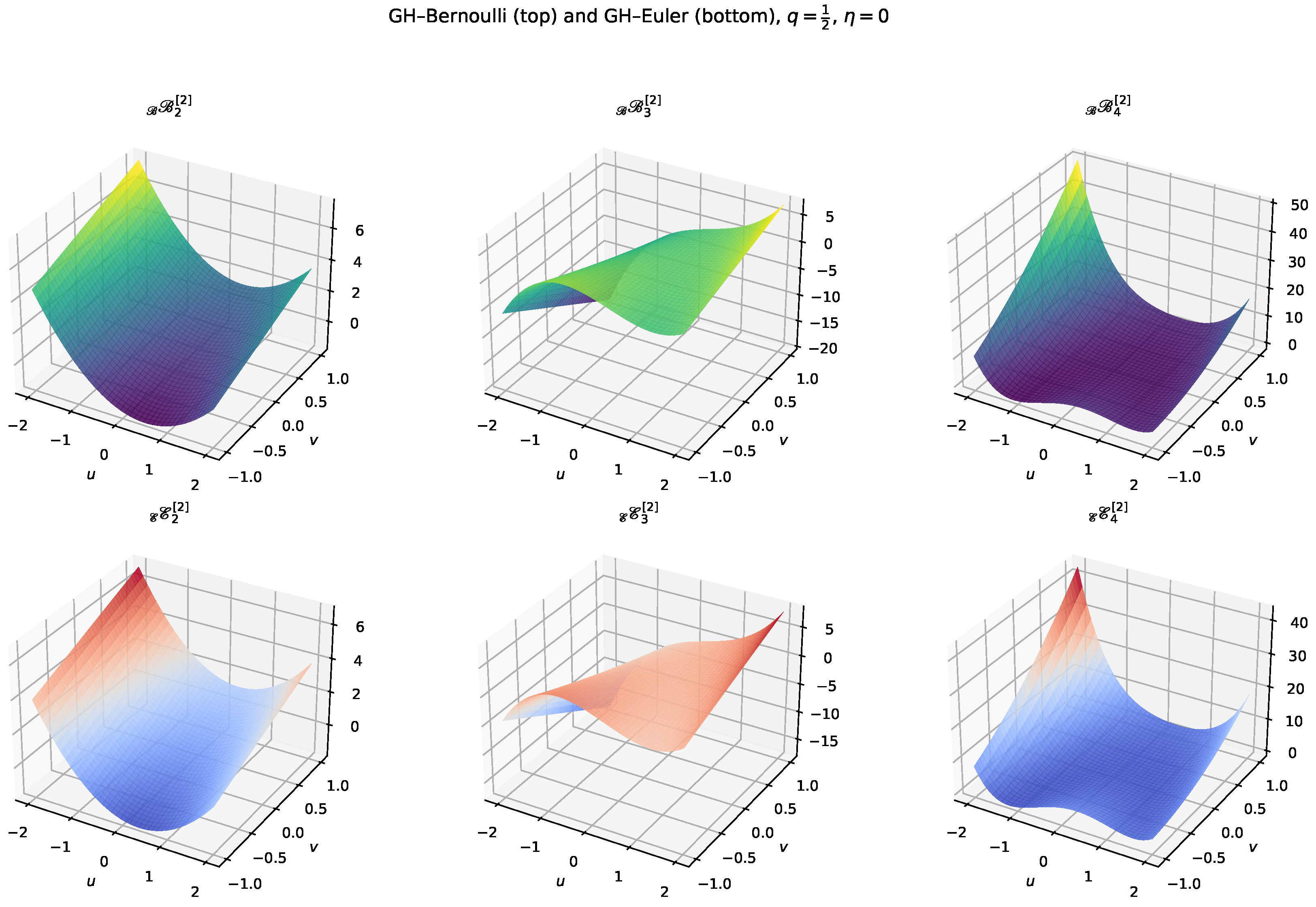
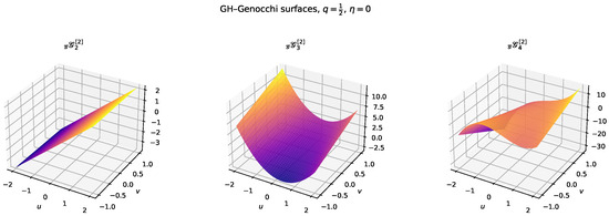
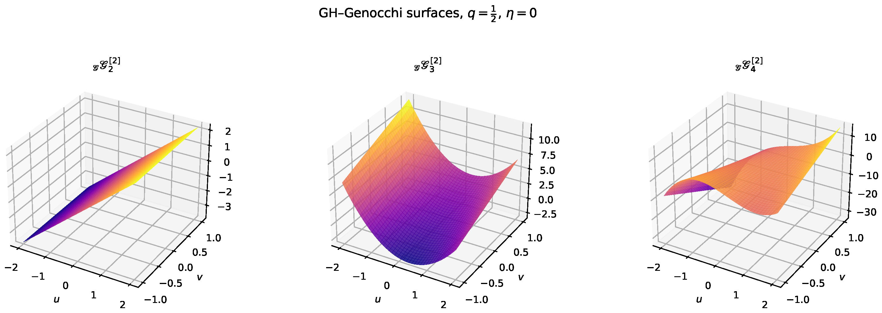
Figure 4 shows the surfaces of the GH–Bernoulli (top row) and GH–Euler (bottom row) polynomials for $n=2,3,4$; the downward shift of the Bernoulli surfaces relative to the Euler surfaces directly visualises the sign difference between the Bernoulli number ${\mathfrak{b}}_1\approx -0.667$ and the Euler number ${\mathfrak{e}}_1=-0.5$. Figure 5 shows the Genocchi family; the scaling factor ${⟨n⟩}_{1/2}$ in (41) is clearly visible as an amplitude magnification relative to the Euler surfaces, and the absence of a $n=0$ surface reflects ${}_{\mathcal{G}}\mathcal{G}_{0;q,\eta }^{\left[j\right]}=0$.

Figure 4. Surfaces of ${}_{\mathcal{G}}\mathcal{B}_{n;1/2,0}^{\left[2\right]}(u,v)$ ((top), viridis) and ${}_{\mathcal{G}}\mathcal{E}_{n;1/2,0}^{\left[2\right]}(u,v)$ ((bottom), coolwarm) for $n=2,3,4$ over $[-2,2]\times [-1,1]$, computed via (42) and (43), $q=\frac{1}{2}$, $\eta =0$.

Figure 5. Surfaces of ${}_{\mathcal{G}}\mathcal{G}_{n;1/2,0}^{\left[2\right]}(u,v)$ for $n=2,3,4$ over $[-2,2]\times [-1,1]$, computed via (44), $q=\frac{1}{2}$, $\eta =0$.

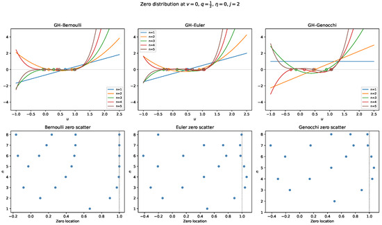
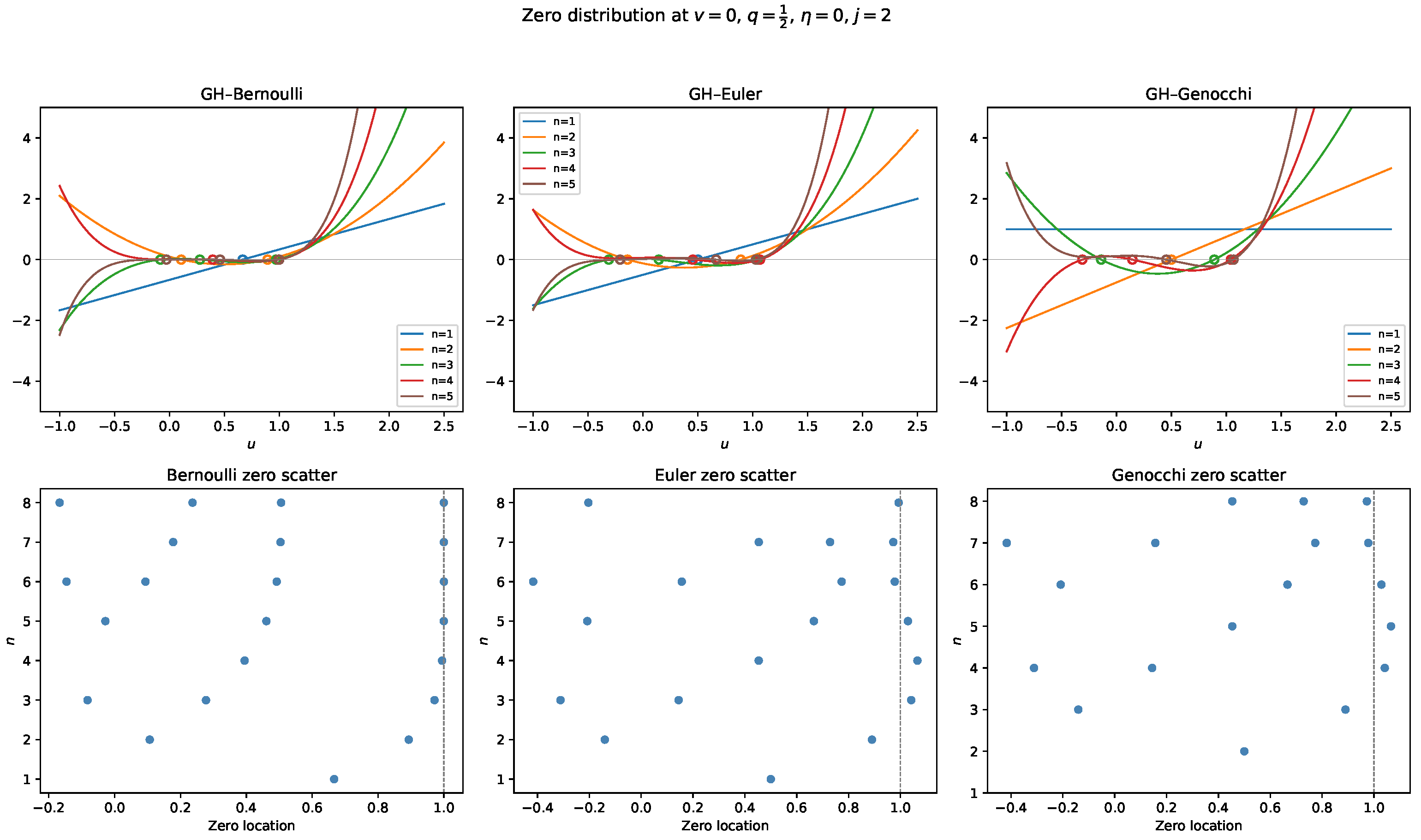
Table 6 records the real zeros of the three families for $n=1,\dots ,5$ at $v=0$, $q=\frac{1}{2}$, $\eta =0$; the data confirm the Genocchi–Euler zero-coincidence of Corollary 12 and illustrate the Genocchi–Euler zero correspondence. For the displayed Bernoulli data, most real zeros lie in $[0,1]$, but small negative roots occur for $n=3$ and $n=5$; therefore, no general zero-location theorem is claimed.

Table 6. Real zeros at $v=0$, $q=\frac{1}{2}$, $\eta =0$, $j=2$.

n	${}_{\mathcal{G}}\mathcal{B}_{\mathit{n}}^{\left[2\right]}$: Zeros	${}_{\mathcal{G}}\mathcal{E}_{\mathit{n}}^{\left[2\right]}$: Zeros	${}_{\mathcal{G}}\mathcal{G}_{\mathit{n}}^{\left[2\right]}$: Zeros
1	0.6667	0.5000	(none)
2	0.1066, 0.8934	−0.1404, 0.8904	0.5000
3	−0.0824, 0.2775, 0.9716	−0.3113, 0.1445, 1.0418	−0.1404, 0.8904
4	0.3949, 0.9947	0.4535, 1.0659	−0.3113, 0.1445, 1.0418
5	−0.0281, 0.4610, 0.9997	−0.2082, 0.6664, 1.0291	0.4535, 1.0659

The data are purely numerical illustrations: the Bernoulli real zeros are predominantly in $[0,1]$ for the displayed degrees, with the negative values listed in Table 6; the Euler roots show a different displacement pattern; and the Genocchi zeros at order n coincide with the Euler zeros at order $n-1$ by the exact relation (41). Figure 6 shows the polynomial curves with zeros marked (top row) and the zero scatter diagrams for $n=1,\dots ,8$ (bottom row); the scatter diagrams numerically illustrate that many Bernoulli zeros lie near $[0,1]$, while some degrees also possess negative real roots as recorded in Table 6. The Genocchi zeros replicate the Euler zero pattern shifted by one degree, consistently with the exact algebraic relation (41).

Figure 6. (Top): Polynomial curves of ${}_{\mathcal{G}}\mathcal{B}_n^{\left[2\right]}$ (left), ${}_{\mathcal{G}}\mathcal{E}_n^{\left[2\right]}$ (centre), ${}_{\mathcal{G}}\mathcal{G}_n^{\left[2\right]}$ (right) at $v=0$, $q=\frac{1}{2}$, $\eta =0$, for $n=1,\dots ,5$; open circles mark real zeros. (Bottom): Scatter diagrams of zero locations vs. order $n=1,\dots ,8$; dashed vertical line marks $u=1$.

Remark 4 (Scope of the zero study).

The zero plots and Table 6 are numerical illustrations, not a proof of global location, interlacing, or asymptotic properties. They were computed at $v=0$ to isolate the one-variable root geometry. When $v\ne 0$, the coefficients acquire additional terms through the affine Gould–Hopper factor ${\mathcal{E}}_{q,\eta }(v,{\mu }^j)$, so the roots may move, split into real and complex conjugate pairs, or change their clustering pattern as v varies. A rigorous perturbation or zero-counting analysis in the parameter v is beyond the present paper and is identified as a future problem.

5. Conclusions

We have introduced the affine $(q,\eta )$-Hermite-based Appell polynomials of order j and developed a unified algebraic and operator framework. The principal achievements comprise the explicit double-sum series representation (Theorem 1), the lowering and raising ladder operator pair $(P_{q,\eta }^{-},P_{q,\eta }^{+})$ satisfying $P_{q,\eta }^{-}{}_{\mathcal{G}}\mathcal{A}_n^{\left[j\right]}={⟨n⟩}_q{}_{\mathcal{G}}\mathcal{A}_{n-1}^{\left[j\right]}$ and $P_{q,\eta }^{+}{}_{\mathcal{G}}\mathcal{A}_n^{\left[j\right]}={}_{\mathcal{G}}\mathcal{A}_{n+1}^{\left[j\right]}$ with the q-commutator $[P_{q,\eta }^{-},P_{q,\eta }^{+}]{}_{\mathcal{G}}\mathcal{A}_n^{\left[j\right]}=q^n{}_{\mathcal{G}}\mathcal{A}_n^{\left[j\right]}$, the complete quasi-monomial framework ${}_{\mathcal{G}}\mathcal{A}_n^{\left[j\right]}={\left(P_{q,\eta }^{+}\right)}^n\left\{1\right\}$, the affine j-th order diffusion relation on the polynomial family for every admissible invertible multiplier $\mathcal{A}$, and the converse, determinantal, addition, and order-recursion theorems. Specialising to the Bernoulli, Euler, and Genocchi generators (Section 4) yielded the Hermite-based Bernoulli, Euler, and Genocchi polynomial families with explicit generating equations. Bernoulli and Euler inherit the invertible operator theory, whereas Genocchi is handled through the exact Euler relation; numerical tables, surface plots, and a numerical zero-distribution illustration are also provided. The Genocchi–Euler relation ${}_{\mathcal{G}}\mathcal{G}_n^{\left[j\right]}={⟨n⟩}_q{}_{\mathcal{G}}\mathcal{E}_{n-1}^{\left[j\right]}$ was confirmed both analytically and graphically.

The results obtained here open several promising avenues for future research. A natural first direction is the multivariable generalisation obtained by replacing the single kernel ${\mathcal{E}}_{q,\eta }(v,{\mu }^j)$ with a product ${\prod }_{i=1}^r{\mathcal{E}}_{q,\eta }(v_{i+1},{\mu }^i)$, which would produce a multi-index Hermite-based Appell hierarchy whose structural theory is expected to parallel the bivariate development presented here. A second direction concerns $(p,q)$-analogues: applying the two-parameter framework of Sadjang [19] should yield a richer algebraic structure with additional symmetry properties between the two base parameters. Third, the study of operational semigroups—in particular, finding the $(q,\eta )$-analogue of $e^{v{\partial }^j}$—would provide a rigorous functional-analytic underpinning for the raising and lowering operators developed in this work. Fourth, it is natural to investigate whether particular parameter choices or sub-families admit orthogonality or d-orthogonality. No orthogonality property is asserted for the general Appell family; any such property would require separate conditions on the multiplier and parameters. Fifth, establishing precise zero-asymptotic laws for the real-zero locations as $n\to \infty$ would complement the numerical and graphical zero study of Section 4 with rigorous asymptotic estimates. Another possible extension, as suggested by the reviewer, is to compare the present q-factorial operator framework with the $S_M$-type and $\varrho$-Weyl fractional constructions of Hadi et al. [24]. In particular, one may ask whether such a kernel can serve as an admissible multiplier, or whether a fractional analogue of the affine diffusion relation can be formulated consistently.

Finally, a systematic investigation of the dependence on j—how the zero distribution, the diffusion-equation structure, and the quasi-monomial properties evolve as j varies from 2 to larger integers—would deepen the understanding of the role of the Gould–Hopper order parameter in the theory of special functions of mathematical physics.

References

- Gould, H.W.; Hopper, A.T. Operational formulas connected with two generalizations of Hermite polynomials. Duke Math. J. 1962, 29, 51–63. [Google Scholar] [CrossRef] [Scilit]
- Steffensen, J.F. The poweroid, an extension of the mathematical notion of power. Acta Math. 1941, 73, 333–366. [Google Scholar] [CrossRef] [Scilit]
- Costabile, F.A.; Dell’Accio, F.; Gualtieri, M.I. A new approach to Bernoulli polynomials. Rend. Mat. Appl. 2006, 26, 1–12. [Google Scholar]
- Dattoli, G. Hermite–Bessel and Laguerre–Bessel functions: A by-product of the monomiality principle. In Advanced Special Functions and Applications; (Melfi, 1999); Aracne: Rome, Italy, 2000; pp. 147–164. [Google Scholar]
- Appell, P. Sur une classe de polynômes. Ann. Sci. l’École Norm. Supérieure 1880, 9, 119–144. [Google Scholar] [CrossRef] [Scilit]
- Annaby, M.H.; Hamza, A.E.; Aldwoah, K.A. Hahn difference operator and associated Jackson–Nörlund integrals. J. Optim. Theory Appl. 2012, 154, 133–153. [Google Scholar] [CrossRef] [Scilit]
- Ernst, T. More expansion formulas for q, η-Apostol Bernoulli and Euler polynomials. Commun. Korean Math. Soc. 2020, 35, 417–445. [Google Scholar] [CrossRef]
- Ernst, T. A Comprehensive Treatment of q-Calculus; Birkhäuser/Springer: Basel, Switzerland, 2012. [Google Scholar]
- Ernst, T. On three general q, η-Apostol polynomials and their connection to q, η-power sums. Adv. Dyn. Syst. Appl. 2019, 14, 119–148. [Google Scholar] [CrossRef] [Scilit]
- Varma, S.; Yaşar, B.; Özarslan, M.A. Hahn–Appell polynomials and their d-orthogonality. Rev. Real Acad. Cienc. Exactas Físicas Nat. Ser. A Matemáticas 2019, 113, 2127–2145. [Google Scholar] [CrossRef] [Scilit]
- Khan, W.A.; Yagci, O.; Mohamed, K.S.; Mohamed, M.A.; Mohammed, N. On some properties of degenerate q-derangement numbers and polynomials. AIMS Math. 2026, 11, 15277–15301. [Google Scholar] [CrossRef] [Scilit]
- Khan, W.A.; Yagci, O.; Mohamed, K.S.; Iqbal, A.; Koh, W.S.; Mohammed, N. Sheffer-type lacunary bivariate q-Laguerre polynomials with applications to heterogeneous graph filters. Netw. Heterog. Media 2026, 21, 1393–1425. [Google Scholar] [CrossRef] [Scilit]
- Khan, W.A.; Yagci, O. A degenerate q-hybrid Heine equation and Beta kernel integral representations. Open J. Math. Sci. 2026, 10, 1030–1056. [Google Scholar] [CrossRef] [Scilit]
- Khan, W.A.; Yagci, O.; Mohamed, K.S.; Osman, O.; Mohamed, N. A new generalization of two variable q-Gould–Hopper–Hahn Appell polynomials via quantum q-calculus. Mathematics 2026, 14, 2375. [Google Scholar] [CrossRef] [Scilit]
- Khan, W.A.; Yagci, O.; Mohamed, K.S.; Osman, O. Evaluation of q-truncated exponential based-Hahn Appell polynomials in the framework of quantum calculus. Mathematics 2026, 14, 2403. [Google Scholar] [CrossRef] [Scilit]
- Ben Cheikh, Y. On obtaining dual sequences via quasi-monomiality. Georgian Math. J. 2002, 9, 413–422. [Google Scholar] [CrossRef] [Scilit]
- Özarslan, M.A.; Yılmaz, B. A set of finite order differential equations for the Appell polynomials. J. Comput. Appl. Math. 2014, 259, 108–116. [Google Scholar] [CrossRef] [Scilit]
- Sharma, A.; Chak, A.M. The basic analogue of a class of polynomials. Riv. Mat. Univ. Parma 1954, 5, 325–337. [Google Scholar]
- Njionou Sadjang, P. On (p, q)-Appell polynomials. Anal. Math. 2019, 45, 583–598. [Google Scholar]
- Wani, S.A.; Warke, A.; Dar, J.G. Degenerate 2D bivariate Appell polynomials: Properties and applications. Appl. Math. Sci. Eng. 2023, 31, 2194645. [Google Scholar] [CrossRef] [Scilit]
- Alyusof, R.; Wani, S.A. Certain properties and applications of Δh hybrid special polynomials associated with Appell sequences. Fractal Fract. 2023, 7, 233. [Google Scholar] [CrossRef] [Scilit]
- Ramírez, W.; Cesarano, C.; Wani, S.A.; Yousuf, S.; Bedoya, D. About properties and the monomiality principle of Bell-based Apostol–Bernoulli-type polynomials. Carpathian Math. Publ. 2024, 16, 379–390. [Google Scholar] [CrossRef] [Scilit]
- Costabile, F.A.; Longo, E. A determinantal approach to Appell polynomials. J. Comput. Appl. Math. 2010, 234, 1528–1542. [Google Scholar] [CrossRef] [Scilit]
- Hadi, S.H.; Challab, K.A.; Ali, A.H.; Alatawi, A.A. A ϱ-Weyl fractional operator of the extended S-type function in a complex domain. MethodsX 2024, 13, 103061. [Google Scholar] [CrossRef] [Scilit] [PubMed]
Disclaimer/Publisher’s Note: The statements, opinions and data contained in all publications are solely those of the individual author(s) and contributor(s) and not of MDPI and/or the editor(s). MDPI and/or the editor(s) disclaim responsibility for any injury to people or property resulting from any ideas, methods, instructions or products referred to in the content. |
© 2026 by the authors. Licensee MDPI, Basel, Switzerland. This article is an open access article distributed under the terms and conditions of the Creative Commons Attribution (CC BY) license.