Stability and Transient Dynamics of a Distributed-Order Fractional SEIRS Epidemic Model with Temporary Immunity

Abstract

This paper investigates a distributed-order fractional SEIRS epidemic model with temporary immunity, vaccination, disease-induced mortality, and density-dependent natural mortality. The distributed-order formulation provides a flexible framework for incorporating heterogeneous memory effects into epidemic dynamics. The basic reproduction number is derived, the disease-free and endemic equilibria are characterized, and their local stability properties are investigated through the distributed-order characteristic equation. In addition, a sufficient global disease extinction criterion is established using a distributed-order Lyapunov argument, yielding global asymptotic stability of the disease-free equilibrium under an explicit transmission bound. Numerical spectral analysis shows that no oscillatory stability transition occurs within the considered parameter ranges and that the endemic equilibrium remains asymptotically stable within these ranges. Numerical simulations examine the effects of the memory interval and memory density shape on epidemic transients. Broadening the memory interval toward lower fractional orders slows convergence and increases transient persistence. For a fixed memory interval, densities concentrated near lower fractional orders produce the slowest relaxation, whereas those concentrated near higher orders, closer to the classical first-order limit, yield the fastest decay. These results show that distributed-order memory primarily regulates transient epidemic dynamics while preserving endemic equilibrium stability within the investigated parameter regimes, providing new insight into heterogeneous memory effects in fractional epidemic models.

1. Introduction

Mathematical models play a fundamental role in understanding disease transmission, threshold behavior, persistence, and control. Since the development of classical compartmental models, epidemic formulations have evolved from SIR and SEIR structures to SIRS and SEIRS models that account for waning immunity and recurrent susceptibility [1,2,3]. Such extensions are particularly relevant for infectious diseases in which immunity following infection or vaccination is incomplete, temporary, or variable. Recent studies have further emphasized the importance of waning and variable immunity in shaping epidemic dynamics and disease persistence [4,5]. Moreover, incorporating density-dependent demographic effects improves biological realism by allowing population size to influence mortality and long-term disease dynamics. Consequently, SEIRS models with temporary immunity provide an appropriate framework for investigating reinfection-driven epidemics under realistic demographic conditions. Fractional SEIR-type models with density-dependent mortality have further demonstrated the usefulness of combining memory effects with biologically realistic epidemic mechanisms [6,7]. Most classical epidemic models employ integer-order derivatives and therefore describe disease evolution solely through the current state of the system. However, transmission, latency, recovery, immune waning, and behavioral responses may depend on past history, motivating the use of fractional operators with memory. Fractional-order epidemic models provide a natural framework for representing such hereditary effects and can produce richer transient dynamics than their integer-order counterparts. Recent studies and reviews further emphasize the growing role of memory effects and fractional modeling in mathematical epidemiology [8,9].

Despite these advances, conventional single-order fractional models employ a single memory exponent throughout the system, which may be inadequate when biological processes exhibit multiple memory scales. Such heterogeneity may arise from differences in immune waning, vaccination-induced protection, or behavioral responses. Variable-order and distributed-order fractional operators provide a more flexible framework by allowing the memory effect to vary with time, state, or a weighted continuum of fractional orders. Recent studies have demonstrated their potential for modeling heterogeneous nonlocal dynamics more realistically than constant-order formulations [10,11]. The transition from single-order to distributed-order models also introduces significant mathematical challenges because stability depends on an entire memory distribution rather than a single fractional exponent. Consequently, considerable attention has been devoted to developing stability theory for distributed-order differential equations and linear systems, together with numerical methods for approximating distributed-order operators and their spectral properties [12,13,14]. These developments provide the theoretical foundation for determining whether distributed memory alters the asymptotic stability of epidemic equilibria or primarily influences the decay rate and persistence of transient dynamics.

Although distributed-order fractional models have received increasing attention, their application to epidemic modeling remains limited. A recent distributed-order hantavirus model demonstrates the potential of this framework for infectious-disease dynamics [15]. In particular, fractional SVEIR models have been examined from the perspective of global stability, whereas delay-based epidemic models with temporary immunity have shown that immune waning and boosting may induce stability switches and oscillatory behavior [16,17]. Nevertheless, these studies do not fully explain how a distributed spectrum of memory orders influences endemic equilibrium stability and transient epidemic dynamics in demographic SEIRS models. Motivated by this gap, the present work considers a distributed-order fractional SEIRS model incorporating temporary immunity, vaccination, disease-induced mortality, and density-dependent natural mortality. Particular attention is given to how the memory interval and memory density function influence local stability and transient relaxation. Unlike previous studies, which primarily focus on threshold analysis, existence, or single-order formulations, the proposed framework systematically investigates the role of heterogeneous distributed memory in governing the damping, persistence, and accumulated magnitude of epidemic transients.

Recent advances further illustrate the growing scope of fractional epidemic modeling. Fractional and distributed-order formulations have been applied to investigate global epidemic dynamics, stability, and memory effects in SIRS and SEIR-type models [18,19]. Fractional epidemic models have also been integrated with optimal control frameworks to evaluate vaccination, treatment, and non-pharmaceutical intervention strategies in both compartmental and spatiotemporal settings [20,21,22]. In addition, fractional models with vaccination have provided further evidence that memory effects play an important role in disease transmission, persistence, and control [23]. Collectively, these studies demonstrate the broad applicability of fractional epidemic models while highlighting the need for further investigation of distributed-order memory effects in SEIRS systems with temporary immunity.

Among the classical epidemic models with temporary immunity, the SEIRS model of Greenhalgh [24] established that latent infection and waning immunity may induce Hopf bifurcation and sustained oscillatory dynamics. Building on this framework, the present work incorporates distributed-order fractional memory to investigate heterogeneous hereditary effects within the same epidemiological setting. Although substantial progress has been made in fractional epidemic modeling, distributed-order SEIRS models simultaneously accounting for temporary immunity, vaccination, disease-induced mortality, and density-dependent natural mortality remain largely unexplored. In particular, it is still unclear whether distributed-order memory fundamentally alters the local stability of the endemic equilibrium or primarily affects the decay rate and persistence of epidemic transients. Motivated by this gap, we develop and analyze a distributed-order fractional SEIRS model, derive its threshold dynamics and equilibrium structure, and systematically investigate how the memory interval and memory density function influence endemic equilibrium stability and transient relaxation. The proposed framework provides a flexible description of heterogeneous memory effects and offers new insights into their role in epidemic dynamics. Recent developments in nonlinear fractional-order systems have also employed Lyapunov-based techniques, fractional differential inequalities, and Mittag–Leffler stability criteria to establish stability and synchronization conditions for complex dynamical systems [25]. These approaches further demonstrate the importance of stability tools specifically adapted to the nonlocal memory structure of fractional-order models.

The main contributions of this work are threefold. First, a distributed-order fractional SEIRS model is formulated that simultaneously incorporates temporary immunity, vaccination, disease-induced mortality, and density-dependent natural mortality, thereby extending the corresponding classical SEIRS framework to heterogeneous memory. Second, the basic reproduction number and local stability properties of the equilibria are analyzed through the distributed-order characteristic symbol ${\Psi }_{\omega }\left(s\right)$, while a sufficient global disease extinction criterion is established using a distributed-order Lyapunov argument. Explicit conditions for possible oscillatory stability transitions of the endemic equilibrium are also derived. Third, the separate effects of the support and shape of the memory distribution are systematically quantified, showing that distributed-order memory can substantially modify transient damping, persistence, and relaxation while preserving endemic equilibrium stability within the investigated parameter ranges.

The remainder of this paper is organized as follows. Section 2 presents the distributed-order fractional SEIRS model. Section 3 develops the qualitative analysis, including the equilibrium, local stability, and global disease extinction results. Section 4 investigates memory-induced oscillatory stability transitions. Section 5 reports the numerical simulations and discussion, Section 6 analyzes the sensitivity to distributed-order memory, and Section 7 concludes the paper.

2. Formulation of the Distributed-Order Fractional SEIRS Model

2.1. General Model Formulation

The proposed model extends the classical SEIRS epidemic model by replacing the first-order time derivative with a distributed-order Caputo fractional derivative, thereby incorporating multiple memory scales into the epidemic dynamics while preserving the biological mechanisms of the original formulation. The model considers a population divided into four epidemiological compartments: susceptible $X\left(t\right)$, exposed (latent) $H\left(t\right)$, infectious $Y\left(t\right)$, and temporarily immune $Z\left(t\right)$ individuals. The total population size is

$$N\left(t\right)=X\left(t\right)+H\left(t\right)+Y\left(t\right)+Z\left(t\right).$$

(1)

The model assumes homogeneous mixing, no vertical transmission, temporary immunity, vaccination, and density-dependent demographic effects. Newborn individuals enter the susceptible class at a per capita birth rate r, while a fraction q is successfully vaccinated at birth. In addition, susceptible individuals may receive vaccination at rate p, which transfers them from $X\left(t\right)$ to the temporarily immune class $Z\left(t\right)$. Disease transmission occurs through the incidence function $\beta \left(N\right)XY/N$, where $\beta \left(N\right)$ denotes the population-dependent contact rate. Exposed individuals progress to the infectious class at rate $\sigma$, and infectious individuals recover at rate $\gamma$. The class $Z\left(t\right)$ is treated as an aggregated temporarily immune compartment containing individuals protected through either recovery or vaccination; accordingly, $\epsilon$ is interpreted as an effective immunity-loss rate for this combined class. Individuals in $Z\left(t\right)$ lose protection at rate $\epsilon$ and return to the susceptible class. All individuals experience density-dependent natural mortality $f\left(N\right)$, whereas infectious individuals are subject to an additional disease-induced mortality rate $\mu$. For mathematical well-posedness, we assume that $\beta ,f:{\mathbb{R}}_{+}\to {\mathbb{R}}_{+}$ are locally Lipschitz continuous. In addition, f is assumed to be strictly increasing, with $f\left(0\right)=0$, and to admit a unique $K>0$ satisfying $f\left(K\right)=r$. These assumptions provide the required local regularity of the nonlinear terms for the existence and uniqueness of solutions and are consistent with the density-dependent demographic formulation used below. To incorporate heterogeneous memory effects, each classical time derivative is replaced by the distributed-order Caputo derivative

$${}^C\mathcal{D}_{0,t}^{\left(\omega \right)}u\left(t\right)={\int }_{{\alpha }_1}^{{\alpha }_2}\omega \left(\alpha \right)T_c^{\alpha -1}{}^{C}D_{0,t}^{\alpha }u\left(t\right)d\alpha ,0<{\alpha }_1<{\alpha }_2\le 1,$$

(2)

Here, $T_c>0$ denotes a characteristic time scale introduced to ensure dimensional consistency of the distributed-order operator. Since ${}^{C}D_{0,t}^{\alpha }u$ has physical dimension $\left[u\right]T^{-\alpha }$, the factor $T_c^{\alpha -1}$ ensures that $T_c^{\alpha -1}{}^{C}D_{0,t}^{\alpha }u$ has the common dimension $\left[u\right]T^{-1}$ for every $\alpha$. Consequently, all contributions in the distributed-order integral have the same physical dimension. The function $\omega \left(\alpha \right)\ge 0$ is a dimensionless normalized memory density function satisfying

$${\int }_{{\alpha }_1}^{{\alpha }_2}\omega \left(\alpha \right)d\alpha =1.$$

(3)

In the present formulation, the same memory density $\omega \left(\alpha \right)$ is used for all compartments as a modeling assumption representing a common population-level memory structure. This choice allows the effects of distributed-order memory to be investigated without introducing additional compartment-specific memory distributions and parameters. Thus, the heterogeneity considered here refers to the spectrum of fractional orders within $\omega \left(\alpha \right)$ rather than to different memory laws across compartments.

The choice of the distributed-order Caputo operator is motivated by both mathematical and biological considerations. Mathematically, it extends the classical Caputo derivative by superposing a continuum of fractional orders through the memory density function $\omega \left(\alpha \right)$, thereby allowing multiple memory scales to be represented within a single operator. It retains the Caputo power-law memory structure at each fractional order while integrating these contributions over a weighted spectrum of orders. Moreover, the Caputo-based formulation accommodates initial conditions in terms of the usual integer-order state values, which is particularly convenient for compartmental epidemic models [26]. The scaling factor $T_c^{\alpha -1}$ introduced in the distributed-order operator ensures dimensional consistency across the different fractional orders. This construction differs from both conventional single-order fractional derivatives and more recently introduced nonsingular-kernel operators. The classical Caputo derivative employs a singular power-law kernel and represents memory through a single fractional order, whereas the Caputo–Fabrizio derivative replaces the power-law kernel by a nonsingular exponential kernel [27]. The Atangana–Baleanu derivative, in turn, employs a nonlocal and nonsingular Mittag–Leffler-type kernel [28]. In contrast, the distributed-order Caputo formulation represents heterogeneous memory through a weighted continuum of fractional orders and can therefore incorporate multiple memory scales without prescribing either a single fractional order or a single nonsingular kernel.

Biologically, epidemic processes such as infection progression, recovery, immune waning, and vaccination-induced protection may involve memory effects operating over different time scales. Representing memory through a distribution of fractional orders provides a natural population-level description of such heterogeneous temporal effects without imposing a single memory exponent on the epidemic dynamics. The distributed-order Caputo operator is therefore particularly suitable for the present SEIRS framework because it incorporates multiple memory scales while preserving the biological structure and conventional initial-value interpretation of the model. Allowing distinct memory densities for individual epidemiological compartments constitutes a natural extension of the present framework. The resulting distributed-order fractional SEIRS model is therefore given by

$$\begin{array}{cc}\hfill {}^C\mathcal{D}_{0,t}^{\left(\omega \right)}X& =r(1-q)N-{\displaystyle \frac{\beta \left(N\right)XY}{N}}-\left(f\left(N\right)+p\right)X+\epsilon Z,\hfill \\ \hfill {}^C\mathcal{D}_{0,t}^{\left(\omega \right)}H& ={\displaystyle \frac{\beta \left(N\right)XY}{N}}-\left(\sigma +f\left(N\right)\right)H,\hfill \\ \hfill {}^C\mathcal{D}_{0,t}^{\left(\omega \right)}Y& =\sigma H-\left(\gamma +\mu +f\left(N\right)\right)Y,\hfill \\ \hfill {}^C\mathcal{D}_{0,t}^{\left(\omega \right)}Z& =rqN+\gamma Y-\left(f\left(N\right)+\epsilon \right)Z+pX.\hfill \end{array}$$

(4)

Here, $X\left(t\right)$, $H\left(t\right)$, $Y\left(t\right)$, and $Z\left(t\right)$ denote the susceptible, exposed (latent), infectious, and temporarily immune populations, respectively, with $N\left(t\right)=X\left(t\right)+H\left(t\right)+Y\left(t\right)+Z\left(t\right)$. The parameter r is the per capita birth rate, q is the fraction successfully vaccinated at birth, p is the booster vaccination rate, $\beta \left(N\right)$ is the population-dependent contact rate, $\sigma$ is the progression rate from the exposed to the infectious class, $\gamma$ is the recovery rate, $\epsilon$ is the immunity-loss rate, $f\left(N\right)$ is the density-dependent natural mortality rate, and $\mu$ is the disease-induced mortality rate. The operator ${}^C\mathcal{D}_{0,t}^{\left(\omega \right)}$ denotes the distributed-order Caputo fractional derivative, $\alpha$ denotes the fractional order, and the parameters ${\alpha }_1$ and ${\alpha }_2$ define the lower and upper bounds of the fractional-order interval. The function $\omega \left(\alpha \right)$ is the normalized memory density function that determines the relative contribution of each fractional order to the distributed-order derivative.

The classical SEIRS formulation of Greenhalgh is recovered as the limiting concentrated memory case in which the normalized memory distribution converges weakly to a Dirac measure at the integer order $\alpha =1$, formally written as $\omega \left(\alpha \right)\to \delta (\alpha -1)$. In this limit, ${}^C\mathcal{D}_{0,t}^{\left(\omega \right)}u\left(t\right)\to du/dt$. Thus, the present framework generalizes the classical model by incorporating distributed memory while preserving its epidemiological structure.

2.2. Results for a Constant Contact Rate

We first consider the distributed-order fractional SEIRS model (4) under the assumption that the contact rate is constant, namely,

$$\beta \left(N\right)\equiv \beta ,\beta >0,$$

(5)

so that the incidence term becomes

$$\beta {\displaystyle \frac{XY}{N}}.$$

Throughout this subsection, the natural mortality function f is assumed to be continuously differentiable and strictly increasing. Unlike the classical integer-order formulation, the analysis is carried out directly in terms of the population variables $(X,H,Y,Z)$ because the distributed-order Caputo derivative does not satisfy the classical quotient rule. Consequently, no distributed-order system is derived for the population proportions $X/N$, $H/N$, $Y/N$, and $Z/N$. The total population is therefore given by

$$N=X+H+Y+Z.$$

2.2.1. Disease-Free Population State and Reproduction Number

In the absence of infection,

$$H=Y=0,$$

$${}^C\mathcal{D}_{0,t}^{\left(\omega \right)}N=\left(r-f\left(N\right)\right)N.$$

(6)

Besides the extinction equilibrium $N=0$, a positive disease-free population level exists whenever

$$f\left(K\right)=r.$$

(7)

Since f is strictly increasing, the positive solution is unique and is given by

$$K=f^{-1}\left(r\right).$$

At the disease-free equilibrium,

$$X_0+Z_0=K,$$

and

$$0=r(1-q)K-(r+p)X_0+\epsilon Z_0.$$

Hence,

$$X_0=K{\displaystyle \frac{r(1-q)+\epsilon }{p+r+\epsilon }},Z_0=K{\displaystyle \frac{p+rq}{p+r+\epsilon }}.$$

(8)

Therefore, the positive disease-free equilibrium is

$${\mathcal{E}}_0=\left(X_0,0,0,Z_0\right),N_0=K.$$

(9)

To derive the epidemic threshold, we linearize the infected subsystem $(H,Y)$ about ${\mathcal{E}}_0$, obtaining

$${}^C\mathcal{D}_t^{\left(\omega \right)}\left(\begin{array}{c}H\\ Y\end{array}\right)=(\mathcal{F}-\mathcal{V})\left(\begin{array}{c}H\\ Y\end{array}\right),$$

(10)

where

$$\mathcal{F}=\left(\begin{array}{cc}0& {\displaystyle \beta \frac{X_0}{K}}\\ 0& 0\end{array}\right),$$

and

$$\mathcal{V}=\left(\begin{array}{cc}\sigma +r& 0\\ -\sigma & \gamma +\mu +r\end{array}\right).$$

The corresponding next-generation matrix is

$$\mathcal{F}{\mathcal{V}}^{-1}=\left(\begin{array}{cc}{\displaystyle \frac{\beta \sigma X_0}{K(\sigma +r)(\gamma +\mu +r)}}& {\displaystyle \frac{\beta X_0}{K(\gamma +\mu +r)}}\\ 0& 0\end{array}\right).$$

The following result provides the basic reproduction number.

Theorem 1.

Assume that the contact rate is constant and that f is continuously differentiable and strictly increasing. Then, the distributed-order fractional SEIRS model admits the positive disease-free equilibrium ${\mathcal{E}}_0=(X_0,0,0,Z_0)$ given by (8) and (9). Moreover, the basic reproduction number is

$${\mathcal{R}}_0=\rho \left(\mathcal{F}{\mathcal{V}}^{-1}\right)={\displaystyle \frac{\beta \sigma \left[r(1-q)+\epsilon \right]}{(\sigma +r)(\gamma +\mu +r)(p+r+\epsilon )}}.$$

(11)

The basic reproduction number ${\mathcal{R}}_0$ represents the expected number of secondary infectious cases generated by a single infectious individual introduced into a disease-free population. Specifically,

$${\displaystyle \frac{r(1-q)+\epsilon }{p+r+\epsilon }}={\displaystyle \frac{X_0}{K}}$$

is the susceptible fraction at the disease-free equilibrium,

$${\displaystyle \frac{\sigma }{\sigma +r}}$$

is the probability that an exposed individual survives the latent stage and becomes infectious, and

$${\displaystyle \frac{1}{\gamma +\mu +r}}$$

is the mean infectious period. Consequently, ${\mathcal{R}}_0<1,$ corresponds to disease extinction, whereas ${\mathcal{R}}_0>1,$ permits invasion of the disease-free equilibrium by a small infectious population.

2.2.2. Biological Time-Scale Condition

The following biological time-scale assumption will be used throughout the equilibrium and stability analysis. The mean duration of temporary immunity is not shorter than either the mean latent period or the mean infectious period, namely,

$$\epsilon \le \sigma +r,\epsilon \le \gamma +\mu +r.$$

(12)

Equivalently,

$${\displaystyle \frac{1}{\epsilon }}\ge {\displaystyle \frac{1}{\sigma +r}},{\displaystyle \frac{1}{\epsilon }}\ge {\displaystyle \frac{1}{\gamma +\mu +r}}.$$

Thus, immunity is retained on average for at least as long as the effective latent and infectious stages. This assumption is the distributed-order analogue of the corresponding time-scale condition in the classical SEIRS model.

2.2.3. Disease-Free and Endemic Equilibria

The existence of the disease-free and endemic equilibria is summarized in the following theorem.

Theorem 2.

Assume that

$$f\left(0\right)<r<f(\infty ),$$

with f continuously differentiable and strictly increasing, so that the positive carrying capacity

$$K=f^{-1}\left(r\right)$$

exists. Then,

(i) 

The model possesses the unique positive disease-free equilibrium

$${\mathcal{E}}_0=(X_0,0,0,Z_0),$$

given by (8) and (9).

(ii) 

If ${\mathcal{R}}_0<1,$ then ${\mathcal{E}}_0$ is locally asymptotically stable under the admissibility conditions for the distributed-order characteristic symbol ${\Psi }_{\omega }$.

(iii) 

If ${\mathcal{R}}_0>1,$ then ${\mathcal{E}}_0$ is unstable.

(iv) 

Every endemic equilibrium

$${\mathcal{E}}^{\ast }=(X^{\ast },H^{\ast },Y^{\ast },Z^{\ast }),N^{\ast }>0,$$

satisfies

$${\displaystyle \frac{X^{\ast }}{N^{\ast }}}={\displaystyle \frac{(\sigma +f\left(N^{\ast }\right))(\gamma +\mu +f\left(N^{\ast }\right))}{\beta \sigma }},$$

(13)

$$H^{\ast }={\displaystyle \frac{\gamma +\mu +f\left(N^{\ast }\right)}{\sigma }}{Y}^{\ast },$$

(14)

$$Z^{\ast }={\displaystyle \frac{rq{N}^{\ast }+\gamma Y^{\ast }+p{X}^{\ast }}{f\left(N^{\ast }\right)+\epsilon }},$$

(15)

and

$$(r-f\left(N^{\ast }\right))N^{\ast }=\mu Y^{\ast }.$$

(16)

Proof. 

The disease-free equilibrium follows directly from (6). Since f is strictly increasing, $f\left(N\right)=r$ admits the unique positive solution $N=K$. Solving the remaining equilibrium equations yields (8) and hence (9).

To establish the stability of the complete disease-free equilibrium, we consider the full linearization. The infected perturbations $(h,y)$ form an invariant subsystem because, at ${\mathcal{E}}_0$, the linearized $(H,Y)$ equations do not depend on the demographic perturbations. Their Jacobian block is

$$J_I\left({\mathcal{E}}_0\right)=\left(\begin{array}{cc}-(\sigma +r)& {\displaystyle \beta \frac{X_0}{K}}\\ \sigma & -(\gamma +\mu +r)\end{array}\right).$$

Its trace is

$$tr{J}_I=-(\sigma +\gamma +\mu +2r)<0,$$

while

$$\begin{array}{cc}\hfill det{J}_I\left({\mathcal{E}}_0\right)& =(\sigma +r)(\gamma +\mu +r)-\beta \sigma {\displaystyle \frac{X_0}{K}}\hfill \\ \hfill & =(\sigma +r)(\gamma +\mu +r)(1-{\mathcal{R}}_0).\hfill \end{array}$$

(17)

Hence, when ${\mathcal{R}}_0<1$, both eigenvalues of $J_I$ have negative real parts, whereas for ${\mathcal{R}}_0>1$ the infected block possesses an unstable mode.

It remains to examine the demographic modes. Let

$$n\left(t\right)=x\left(t\right)+h\left(t\right)+y\left(t\right)+z\left(t\right)$$

denote the perturbation of the total population. Since

$${}^C\mathcal{D}_{0,t}^{\left(\omega \right)}N=\left(r-f\left(N\right)\right)N-\mu Y,$$

linearization at $N=K$ and $Y=0$ gives

$${}^C\mathcal{D}_{0,t}^{\left(\omega \right)}n=-K{f}^{\prime }\left(K\right)n-\mu y.$$

Moreover, the linearized susceptible equation can be written in the form

$${}^C\mathcal{D}_{0,t}^{\left(\omega \right)}x=\left[r(1-q)+\epsilon -X_0{f}^{\prime }\left(K\right)\right]n-(r+p+\epsilon )x+{\mathcal{C}}_{h}h+{\mathcal{C}}_{y}y,$$

where ${\mathcal{C}}_h$ and ${\mathcal{C}}_y$ are coupling coefficients whose explicit values do not affect the eigenvalues of the demographic block. Thus, with the perturbations ordered as $(h,y,n,x)$, the complete linearized system has the block-triangular form

$$J_0=\left(\begin{array}{cc}{J}_I& 0\\ \ast & J_D\end{array}\right),$$

where

$$J_D=\left(\begin{array}{cc}-K{f}^{\prime }\left(K\right)& 0\\ r(1-q)+\epsilon -X_0{f}^{\prime }\left(K\right)& -(r+p+\epsilon )\end{array}\right).$$

Therefore, the demographic eigenvalues are

$${\lambda }_{D,1}=-K{f}^{\prime }\left(K\right)<0,{\lambda }_{D,2}=-(r+p+\epsilon )<0.$$

Consequently, the spectrum of the complete four-dimensional Jacobian is the union of the spectra of $J_I$ and $J_D$. Hence, for ${\mathcal{R}}_0<1$, all Jacobian modes lie in the stable region and, under the admissibility conditions for the distributed-order characteristic symbol ${\Psi }_{\omega }$, the disease-free equilibrium is locally asymptotically stable. If ${\mathcal{R}}_0>1$, the infected block is unstable and therefore the full disease-free equilibrium is unstable.

At an endemic equilibrium with $Y^{\ast }>0$, the third equilibrium equation immediately gives (14). Substituting this expression into the second equilibrium equation yields (13). The fourth equilibrium equation then gives (15). Finally, summing the four equilibrium equations gives (16). □

3. Qualitative Analysis

3.1. Positivity and Positively Invariant Region

We first establish the biological feasibility of the solutions of system (4). We use the extremum principle for the Caputo fractional derivative and its distributed-order extension [29]. In particular, if a sufficiently regular function u attains a minimum at $t_0>0$, then

$${}^{C}D_{0,t}^{\alpha }u\left(t_0\right)\le 0,0<\alpha \le 1,$$

whereas at a maximum,

$${}^{C}D_{0,t}^{\alpha }u\left(t_0\right)\ge 0.$$

Since $\omega \left(\alpha \right)\ge 0$, the corresponding inequalities are preserved after integration over $[{\alpha }_1,{\alpha }_2]$. Hence,

$${}^C\mathcal{D}_{0,t}^{\left(\omega \right)}u\left(t_0\right)\le 0$$

at a minimum, and

$${}^C\mathcal{D}_{0,t}^{\left(\omega \right)}u\left(t_0\right)\ge 0$$

at a maximum.

Proposition 1.

Let

$$\mathbf{U}\left(t\right)={\left(X\left(t\right),H\left(t\right),Y\left(t\right),Z\left(t\right)\right)}^{\mathsf{T}}$$

be a sufficiently regular solution of system (4) with nonnegative initial conditions. Then

$$X\left(t\right),H\left(t\right),Y\left(t\right),Z\left(t\right)\ge 0,t\ge 0.$$

Consequently, ${\mathbb{R}}_{+}^4$ is positively invariant.

Proof. 

The vector field of system (4) is quasi-positive on the boundary of ${\mathbb{R}}_{+}^4$. Indeed,

$${\left.{}^C\mathcal{D}_{0,t}^{\left(\omega \right)}X\right|}_{X=0}=r(1-q)N+\epsilon Z\ge 0,$$

$${\left.{}^C\mathcal{D}_{0,t}^{\left(\omega \right)}H\right|}_{H=0}={\displaystyle \frac{\beta \left(N\right)XY}{N}}\ge 0,$$

$${\left.{}^C\mathcal{D}_{0,t}^{\left(\omega \right)}Y\right|}_{Y=0}=\sigma H\ge 0,$$

and

$${\left.{}^C\mathcal{D}_{0,t}^{\left(\omega \right)}Z\right|}_{Z=0}=rqN+\gamma Y+pX\ge 0.$$

Thus, whenever one state variable vanishes while the remaining state variables are nonnegative, the corresponding right-hand side is nonnegative. Combining this quasi-positivity property with the extremum principle for the distributed-order Caputo derivative [29] shows that no component can cross from the nonnegative orthant into the negative region. Therefore,

$$X\left(t\right),H\left(t\right),Y\left(t\right),Z\left(t\right)\ge 0,t\ge 0,$$

and hence ${\mathbb{R}}_{+}^4$ is positively invariant. □

We next establish boundedness. Summing the four equations of system (4) gives

$${}^C\mathcal{D}_{0,t}^{\left(\omega \right)}N=\left(r-f\left(N\right)\right)N-\mu Y.$$

(18)

Assume that f is strictly increasing and that the unique positive carrying capacity K satisfies

$$f\left(K\right)=r.$$

Proposition 2.

For every nonnegative solution of system (4),

$$N\left(t\right)\le M,M=max\left\{N\right(0),K\},t\ge 0.$$

In particular, if $N\left(0\right)\le K$, then

$$0\le N\left(t\right)\le K,t\ge 0,$$

and the region

$$\Omega =\left\{(X,H,Y,Z)\in {\mathbb{R}}_{+}^4:X+H+Y+Z\le K\right\}$$

is positively invariant.

Proof. 

By Proposition 1, $Y\left(t\right)\ge 0$, and therefore

$${}^C\mathcal{D}_{0,t}^{\left(\omega \right)}N\le \left(r-f\left(N\right)\right)N.$$

(19)

Let

$$M=max\left\{N\right(0),K\},$$

and, for arbitrary $\delta >0$, define

$$M_{\delta }=M+\delta .$$

Since $M_{\delta }>K$ and f is strictly increasing,

$$r-f\left(M_{\delta }\right)<0.$$

Suppose, for contradiction, that $N\left(t\right)$ reaches $M_{\delta }$ from below at some first time $t_{\delta }>0$. Then

$$N\left(t\right)\le M_{\delta },0\le t\le t_{\delta },N\left(t_{\delta }\right)=M_{\delta },$$

so that N attains a maximum at $t_{\delta }$. By the distributed-order extremum principle [29],

$${}^C\mathcal{D}_{0,t}^{\left(\omega \right)}N\left(t_{\delta }\right)\ge 0.$$

On the other hand, Equation (18) gives

$${}^C\mathcal{D}_{0,t}^{\left(\omega \right)}N\left(t_{\delta }\right)=\left(r-f\left(M_{\delta }\right)\right)M_{\delta }-\mu Y\left(t_{\delta }\right)<0,$$

which is a contradiction. Hence,

$$N\left(t\right)<M_{\delta },t\ge 0.$$

Since $\delta >0$ is arbitrary, letting $\delta \to 0^{+}$ yields

$$N\left(t\right)\le M=max\left\{N\right(0),K\},t\ge 0.$$

If $N\left(0\right)\le K$, then $M=K$, and therefore

$$0\le N\left(t\right)\le K,t\ge 0.$$

Together with Proposition 1, this proves that

$$\Omega =\left\{(X,H,Y,Z)\in {\mathbb{R}}_{+}^4:X+H+Y+Z\le K\right\}$$

is positively invariant. Moreover,

$$0\le X\left(t\right),H\left(t\right),Y\left(t\right),Z\left(t\right)\le K,t\ge 0,$$

for every solution starting in $\Omega$. □

Consequently, the epidemiological compartments remain nonnegative and bounded for nonnegative initial data. In particular, when $N\left(0\right)\le K$, the compact region $\Omega$ provides the natural biologically feasible state space for the subsequent equilibrium and stability analysis.

3.2. Disease-Free and Endemic Equilibria

The equilibrium points of system (4) are obtained by setting the distributed-order Caputo derivatives to zero. Since the distributed-order derivative of a constant vanishes, every equilibrium satisfies the algebraic system

$$\begin{array}{cc}\hfill 0& =r(1-q)N-\beta \left(N\right){\displaystyle \frac{XY}{N}}-\left(f\left(N\right)+p\right)X+\epsilon Z,\hfill \\ \hfill 0& =\beta \left(N\right){\displaystyle \frac{XY}{N}}-\left(\sigma +f\left(N\right)\right)H,\hfill \\ \hfill 0& =\sigma H-\left(\gamma +\mu +f\left(N\right)\right)Y,\hfill \\ \hfill 0& =rqN+\gamma Y+pX-\left(f\left(N\right)+\epsilon \right)Z,\hfill \end{array}$$

(20)

together with

$$N=X+H+Y+Z.$$

Summing the four equilibrium equations yields the total-population relation

$$\left[r-f\left(N\right)\right]N=\mu Y.$$

(21)

Equation (21) shows that the equilibrium population size is directly coupled to the prevalence of infection. In particular, when disease-induced mortality is absent ($\mu =0$), every positive equilibrium satisfies

$$f\left(N\right)=r,$$

whereas for $\mu >0$ the endemic population generally lies below the disease-free carrying capacity.

3.2.1. Disease-Free Equilibrium

Setting

$$H=Y=0$$

in (20) yields

$$f\left(N\right)=r.$$

Assuming that the equation

$$f\left(K\right)=r$$

admits a unique positive solution, the disease-free population size is

$$N=K.$$

The remaining equilibrium equations reduce to

$$r(1-q)K-(r+p)X+\epsilon Z=0,$$

$$rqK+pX-(r+\epsilon )Z=0,$$

together with

$$X+Z=K.$$

Solving these equations gives

$$X_0=K{\displaystyle \frac{r(1-q)+\epsilon }{p+r+\epsilon }},Z_0=K{\displaystyle \frac{p+rq}{p+r+\epsilon }}.$$

(22)

Hence, the unique positive disease-free equilibrium is

$${\mathcal{E}}_0=(X_0,0,0,Z_0).$$

(23)

3.2.2. Endemic Equilibrium

Suppose that

$$Y^{\ast }>0.$$

Then, the equilibrium equations become

$$\begin{array}{cc}\hfill 0& =r(1-q)N^{\ast }-\beta \left(N^{\ast }\right){\displaystyle \frac{X^{\ast }{Y}^{\ast }}{N^{\ast }}}-\left(f\left(N^{\ast }\right)+p\right)X^{\ast }+\epsilon Z^{\ast },\hfill \\ \hfill 0& =\beta \left(N^{\ast }\right){\displaystyle \frac{X^{\ast }{Y}^{\ast }}{N^{\ast }}}-\left(\sigma +f\left(N^{\ast }\right)\right)H^{\ast },\hfill \\ \hfill 0& =\sigma H^{\ast }-\left(\gamma +\mu +f\left(N^{\ast }\right)\right)Y^{\ast },\hfill \\ \hfill 0& =rq{N}^{\ast }+\gamma Y^{\ast }+p{X}^{\ast }-\left(f\left(N^{\ast }\right)+\epsilon \right)Z^{\ast }.\hfill \end{array}$$

(24)

The third equation gives

$$H^{\ast }={\displaystyle \frac{\gamma +\mu +f\left(N^{\ast }\right)}{\sigma }}{Y}^{\ast }.$$

(25)

Substituting this expression into the second equation yields

$${\displaystyle \frac{X^{\ast }}{N^{\ast }}}={\displaystyle \frac{(\sigma +f\left(N^{\ast }\right))(\gamma +\mu +f\left(N^{\ast }\right))}{\beta \left(N^{\ast }\right)\sigma }}.$$

(26)

Similarly, the fourth equation gives

$$Z^{\ast }={\displaystyle \frac{rq{N}^{\ast }+\gamma Y^{\ast }+p{X}^{\ast }}{f\left(N^{\ast }\right)+\epsilon }}.$$

(27)

Finally, (21) becomes

$$\left[r-f\left(N^{\ast }\right)\right]N^{\ast }=\mu Y^{\ast },$$

(28)

which couples the endemic population size with the infectious class. Equations (25)–(28) completely characterize every biologically feasible endemic equilibrium. In general, explicit closed-form expressions are unavailable because both the transmission rate $\beta \left(N\right)$ and the natural mortality function $f\left(N\right)$ depend nonlinearly on the total population size. Consequently, the existence, uniqueness, and stability of endemic equilibria depend on the specific functional forms of $\beta \left(N\right)$ and $f\left(N\right)$ and are investigated in the following subsections under appropriate assumptions.

3.3. Basic Reproduction Number

The basic reproduction number, denoted by ${\mathcal{R}}_0$, is the expected number of secondary infections generated by a single infectious individual introduced into an otherwise disease-free population. It serves as the principal threshold parameter governing disease invasion or extinction. The reproduction number is obtained by applying the next-generation matrix approach to the infected subsystem of system (4). Since the disease-free equilibrium is

$${\mathcal{E}}_0=(X_0,0,0,Z_0),$$

the infected variables are chosen as

$$\mathbf{x}={(H,Y)}^{\mathsf{T}}.$$

The matrices describing the production of new infections and all other transitions are

$$\mathcal{F}=\left(\begin{array}{cc}0& {\displaystyle \beta \left(K\right)\frac{X_0}{K}}\\ 0& 0\end{array}\right),$$

(29)

and

$$\mathcal{V}=\left(\begin{array}{cc}\sigma +r& 0\\ -\sigma & \gamma +\mu +r\end{array}\right),$$

(30)

where $K=f^{-1}\left(r\right)$ denotes the disease-free carrying capacity. The inverse of $\mathcal{V}$ is

$${\mathcal{V}}^{-1}={\displaystyle \frac{1}{(\sigma +r)(\gamma +\mu +r)}}\left(\begin{array}{cc}\gamma +\mu +r& 0\\ \sigma & \sigma +r\end{array}\right).$$

Consequently,

$$\mathcal{F}{\mathcal{V}}^{-1}=\left(\begin{array}{cc}{\displaystyle \frac{\beta \left(K\right)\sigma X_0}{K(\sigma +r)(\gamma +\mu +r)}}& {\displaystyle \frac{\beta \left(K\right)X_0}{K(\gamma +\mu +r)}}\\ 0& 0\end{array}\right),$$

(31)

Since this matrix is upper triangular, its spectral radius is

$${\mathcal{R}}_0={\displaystyle \frac{\beta \left(K\right)\sigma X_0}{K(\sigma +r)(\gamma +\mu +r)}}.$$

(32)

Substituting

$$X_0=K{\displaystyle \frac{r(1-q)+\epsilon }{p+r+\epsilon }},$$

from (22) gives the explicit expression

$${\mathcal{R}}_0={\displaystyle \frac{\beta \left(K\right)\sigma \left[r(1-q)+\epsilon \right]}{(\sigma +r)(\gamma +\mu +r)(p+r+\epsilon )}}.$$

(33)

Equation (33) shows how vaccination, temporary immunity, demographic turnover, and disease-induced mortality jointly influence disease transmission. In particular,

$${\displaystyle \frac{r(1-q)+\epsilon }{p+r+\epsilon }}={\displaystyle \frac{X_0}{K}}$$

is the susceptible fraction of the disease-free population,

$${\displaystyle \frac{\sigma }{\sigma +r}}$$

is the probability that an exposed individual survives the latent stage and becomes infectious, and

$${\displaystyle \frac{1}{\gamma +\mu +r}}$$

is the mean infectious period before recovery, natural death, or disease-induced death. The threshold property of ${\mathcal{R}}_0$ is summarized in the following result.

Theorem 3.

Assume that the disease-free equilibrium ${\mathcal{E}}_0$ exists.

(i) 

If ${\mathcal{R}}_0<1$, each infectious individual generates, on average, fewer than one secondary infection, and disease invasion is not possible.

(ii) 

If ${\mathcal{R}}_0>1$, each infectious individual generates more than one secondary infection, so the disease can invade the disease-free population.

(iii) 

The critical value ${\mathcal{R}}_0=1$ defines the epidemiological threshold separating disease extinction from possible endemic persistence.

It is important to note that the value of ${\mathcal{R}}_0$ does not depend explicitly on the distributed-order weight function $\omega \left(\alpha \right)$. This follows because the next-generation operator is constructed from the equilibrium Jacobian, while the distributed-order Caputo derivative of every constant equilibrium state is zero. Consequently, distributed-order memory influences the transient dynamics and the stability of equilibria through the characteristic equation developed in the following subsections rather than through the value of ${\mathcal{R}}_0$ itself.

3.4. Linearization and a General Stability Criterion

In this subsection, we derive the linearized form of the distributed-order SEIRS model and establish a general criterion for local asymptotic stability. This criterion forms the basis for the stability analysis of both the disease-free and endemic equilibria presented in the following subsections.

Let

$$\mathbf{U}\left(t\right)={\left(X\left(t\right),H\left(t\right),Y\left(t\right),Z\left(t\right)\right)}^{\mathsf{T}},$$

and let

$${\mathbf{U}}^{\ast }={\left(X^{\ast },H^{\ast },Y^{\ast },Z^{\ast }\right)}^{\mathsf{T}}$$

be an equilibrium of (4). Introducing the perturbation

$$\mathbf{u}\left(t\right)=\mathbf{U}\left(t\right)-{\mathbf{U}}^{\ast },$$

and expanding the nonlinear vector field about ${\mathbf{U}}^{\ast }$ gives

$${}^C\mathcal{D}_t^{\left(\omega \right)}\mathbf{u}\left(t\right)=J\left({\mathbf{U}}^{\ast }\right)\mathbf{u}\left(t\right)+\mathcal{O}\left({\parallel \mathbf{u}\parallel }^2\right),$$

(34)

where

$$J\left({\mathbf{U}}^{\ast }\right)={\left[{\displaystyle \frac{\partial F_i}{\partial U_j}}\right]}_{{\mathbf{U}}^{\ast }}$$

denotes the Jacobian matrix of the vector field associated with (4).

Neglecting higher-order terms yields the linearized distributed-order system

$${}^C\mathcal{D}_t^{\left(\omega \right)}\mathbf{u}\left(t\right)=J\left({\mathbf{U}}^{\ast }\right)\mathbf{u}\left(t\right).$$

(35)

Taking the Laplace transform of the linearized system

$${}^C\mathcal{D}_{0,t}^{\left(\omega \right)}\mathbf{u}\left(t\right)=J\left({\mathbf{U}}^{\ast }\right)\mathbf{u}\left(t\right),$$

and using

$$\mathcal{L}\left\{{}^{C}D_{0,t}^{\alpha }\mathbf{u}\left(t\right)\right\}\left(s\right)=s^{\alpha }\widehat{\mathbf{u}}\left(s\right)-s^{\alpha -1}\mathbf{u}\left(0\right),$$

we obtain

$$\left[{\Psi }_{\omega }\left(s\right)I-J\left({\mathbf{U}}^{\ast }\right)\right]\widehat{\mathbf{u}}\left(s\right)={\Phi }_{\omega }\left(s\right)\mathbf{u}\left(0\right),$$

where

$${\Psi }_{\omega }\left(s\right)={\int }_{{\alpha }_1}^{{\alpha }_2}\omega \left(\alpha \right)T_c^{\alpha -1}{s}^{\alpha }d\alpha ,s\in \mathbb{C}\setminus (-\infty ,0],$$

(36)

and

$${\Phi }_{\omega }\left(s\right)={\int }_{{\alpha }_1}^{{\alpha }_2}\omega \left(\alpha \right)T_c^{\alpha -1}{s}^{\alpha -1}d\alpha .$$

Hence,

$$\widehat{\mathbf{u}}\left(s\right)={\left[{\Psi }_{\omega }\left(s\right)I-J\left({\mathbf{U}}^{\ast }\right)\right]}^{-1}{\Phi }_{\omega }\left(s\right)\mathbf{u}\left(0\right).$$

Therefore, the characteristic values governing the linearized dynamics are determined by the singularities of the resolvent

$${\left[{\Psi }_{\omega }\left(s\right)I-J\left({\mathbf{U}}^{\ast }\right)\right]}^{-1},$$

and the corresponding characteristic equation is

$$det\left({\Psi }_{\omega }\left(s\right)I-J\left({\mathbf{U}}^{\ast }\right)\right)=0.$$

(37)

Equation (37) generalizes the classical characteristic polynomial for integer-order epidemic models. In the special case

$$\omega \left(\alpha \right)=\delta (\alpha -1),$$

one has

$${\Psi }_{\omega }\left(s\right)=s,$$

and the characteristic equation reduces to

$$det(sI-J)=0,$$

which is precisely the characteristic equation of the corresponding ordinary differential equation model.

Proposition 3.

Let ${\mathbf{U}}^{\ast }$ be an equilibrium of system (4). Assume that the nonlinear vector field $\mathbf{F}$ is continuously differentiable in a neighborhood of ${\mathbf{U}}^{\ast }$ and admits the local decomposition

$$\mathbf{F}({\mathbf{U}}^{\ast }+\mathbf{u})=J\left({\mathbf{U}}^{\ast }\right)\mathbf{u}+\mathbf{R}\left(\mathbf{u}\right),\parallel \mathbf{R}\left(\mathbf{u}\right)\parallel =o(\parallel \mathbf{u}\parallel )\mathrm{as}\parallel \mathbf{u}\parallel \to 0.$$

Assume further that

$$\omega \left(\alpha \right)\ge 0,{\int }_{{\alpha }_1}^{{\alpha }_2}\omega \left(\alpha \right)d\alpha =1,0<{\alpha }_1<{\alpha }_2\le 1,$$

and define

$${\Psi }_{\omega }\left(s\right)={\int }_{{\alpha }_1}^{{\alpha }_2}\omega \left(\alpha \right)T_c^{\alpha -1}{s}^{\alpha }d\alpha ,s\in \mathbb{C}\setminus (-\infty ,0],$$

using the principal branch of $s^{\alpha }$.

For the linearized system

$${}^C\mathcal{D}_{0,t}^{\left(\omega \right)}\mathbf{u}\left(t\right)=J\left({\mathbf{U}}^{\ast }\right)\mathbf{u}\left(t\right),$$

asymptotic stability holds if and only if every characteristic root of

$$det\left({\Psi }_{\omega }\left(s\right)I-J\left({\mathbf{U}}^{\ast }\right)\right)=0$$

satisfies $Re\left(s\right)<0$. Under the above regularity assumptions, the nonlinear linearization principle for distributed-order fractional systems [30] applies. Consequently, if all characteristic roots lie strictly in the open left half-plane, then the equilibrium ${\mathbf{U}}^{\ast }$ of the nonlinear system is locally asymptotically stable. If the characteristic equation possesses a root with $Re\left(s\right)>0$, then ${\mathbf{U}}^{\ast }$ is unstable.

Proof. 

The Laplace transform calculation developed above gives

$$\widehat{\mathbf{u}}\left(s\right)={\left[{\Psi }_{\omega }\left(s\right)I-J\left({\mathbf{U}}^{\ast }\right)\right]}^{-1}{\Phi }_{\omega }\left(s\right)\mathbf{u}\left(0\right).$$

Hence, the characteristic roots of the linearized system are the zeros of

$$det\left({\Psi }_{\omega }\left(s\right)I-J\left({\mathbf{U}}^{\ast }\right)\right)=0.$$

The stability criterion for linear distributed-order fractional systems implies that the linearized system is asymptotically stable if and only if all these roots lie in the open left half-plane. Since $\mathbf{F}$ is continuously differentiable in a neighborhood of ${\mathbf{U}}^{\ast }$ and $\mathbf{R}\left(\mathbf{u}\right)=o(\parallel \mathbf{u}\parallel )$ as $\parallel \mathbf{u}\parallel \to 0$, the nonlinear terms constitute a higher-order perturbation of the linearized system near the equilibrium. Therefore, by the nonlinear linearization principle for distributed-order fractional systems [30], spectral stability of the linearized system implies local asymptotic stability of ${\mathbf{U}}^{\ast }$. Conversely, the existence of a characteristic root with positive real part implies instability of the equilibrium. □

3.5. Local Stability of the Disease-Free Equilibrium

In this subsection, we apply the general stability criterion established in Proposition 3 to the disease-free equilibrium

$${\mathcal{E}}_0=(X_0,0,0,Z_0),$$

where

$$X_0=K{\displaystyle \frac{r(1-q)+\epsilon }{p+r+\epsilon }},Z_0=K{\displaystyle \frac{p+rq}{p+r+\epsilon }},$$

and $K=f^{-1}\left(r\right)$ denotes the disease-free carrying capacity. Linearizing system (4) about ${\mathcal{E}}_0$ gives

$${}^C\mathcal{D}_{0,t}^{\left(\omega \right)}\mathbf{u}\left(t\right)=J_0\mathbf{u}\left(t\right),$$

where $J_0$ is the Jacobian matrix evaluated at the disease-free equilibrium. The infected perturbations form an invariant subsystem at ${\mathcal{E}}_0$. Hence, the local invasion dynamics are governed by the exposed and infectious compartments, with Jacobian block

$$J_I=\left(\begin{array}{cc}-(\sigma +r)& {\displaystyle \beta \left(K\right)\frac{X_0}{K}}\\ \sigma & -(\gamma +\mu +r)\end{array}\right).$$

(38)

As established in the full linearization of the disease-free equilibrium, the remaining demographic block has eigenvalues

$$-K{f}^{\prime }\left(K\right)\mathrm{and}-(r+p+\epsilon ),$$

which are strictly negative because $K>0$, $f^{\prime }\left(K\right)>0$, and all epidemiological rates are nonnegative. Thus, it remains to determine the stability of the infected block. According to Proposition 3, its characteristic equation is

$$det\left({\Psi }_{\omega }\left(s\right)I-J_I\right)=0,$$

(39)

or equivalently,

$$\left({\Psi }_{\omega }\left(s\right)+\sigma +r\right)\left({\Psi }_{\omega }\left(s\right)+\gamma +\mu +r\right)-{\displaystyle \frac{\beta \left(K\right)\sigma X_0}{K}}=0.$$

(40)

Using

$${\mathcal{R}}_0={\displaystyle \frac{\beta \left(K\right)\sigma X_0}{K(\sigma +r)(\gamma +\mu +r)}},$$

the characteristic equation becomes

$$\left({\Psi }_{\omega }\left(s\right)+\sigma +r\right)\left({\Psi }_{\omega }\left(s\right)+\gamma +\mu +r\right)-(\sigma +r)(\gamma +\mu +r){\mathcal{R}}_0=0.$$

(41)

Theorem 4.

Assume that the hypotheses of Proposition 3 hold, with $\omega \left(\alpha \right)\ge 0$ normalized on $[{\alpha }_1,{\alpha }_2]\subset (0,1]$.

(i) 

If ${\mathcal{R}}_0<1,$ then the disease-free equilibrium ${\mathcal{E}}_0$ is locally asymptotically stable.

(ii) 

If ${\mathcal{R}}_0>1,$ then ${\mathcal{E}}_0$ is unstable.

(iii) 

The critical value ${\mathcal{R}}_0=1$ defines the epidemiological threshold separating disease extinction from possible endemic persistence.

Proof. 

Set

$$a=\sigma +r>0,b=\gamma +\mu +r>0,$$

and write

$$z={\Psi }_{\omega }\left(s\right).$$

Equation (41) is then equivalent to

$$z^2+(a+b)z+ab(1-{\mathcal{R}}_0)=0.$$

(42)

Its two roots are

$$z_{\pm }={\displaystyle \frac{-(a+b)\pm \sqrt{{(a-b)}^2+4ab{\mathcal{R}}_0}}{2}}.$$

(43)

Suppose first that ${\mathcal{R}}_0<1$. Since

$${(a-b)}^2+4ab{\mathcal{R}}_0<{(a-b)}^2+4ab={(a+b)}^2,$$

we have

$$\sqrt{{(a-b)}^2+4ab{\mathcal{R}}_0}<a+b.$$

Consequently,

$$z_{-}<z_{+}<0.$$

We now show that no characteristic root s can lie in the closed right half-plane. Let

$$s=\rho e^{i\theta },\rho >0,\left|\theta \right|\le {\displaystyle \frac{\pi }{2}}.$$

For every $\alpha \in [{\alpha }_1,{\alpha }_2]\subset (0,1]$,

$$Re\left(s^{\alpha }\right)={\rho }^{\alpha }cos\left(\alpha \theta \right)\ge 0.$$

Since $\omega \left(\alpha \right)\ge 0$ and $T_c^{\alpha -1}>0$,

$$Re{\Psi }_{\omega }\left(s\right)={\int }_{{\alpha }_1}^{{\alpha }_2}\omega \left(\alpha \right)T_c^{\alpha -1}{\rho }^{\alpha }cos\left(\alpha \theta \right)d\alpha \ge 0.$$

(44)

Moreover, ${\Psi }_{\omega }\left(0\right)=0$. Therefore, ${\Psi }_{\omega }\left(s\right)$ cannot equal either of the strictly negative real numbers $z_{-}$ and $z_{+}$ for any s satisfying $Re\left(s\right)\ge 0$. Hence, Equation (41) has no characteristic root in the closed right half-plane when ${\mathcal{R}}_0<1$. Together with the strictly stable demographic modes, Proposition 3 implies that the complete disease-free equilibrium ${\mathcal{E}}_0$ is locally asymptotically stable. Now suppose that ${\mathcal{R}}_0>1$. Then

$$ab(1-{\mathcal{R}}_0)<0,$$

so Equation (42) has one positive root, namely $z_{+}>0$. For real $s>0$,

$${\Psi }_{\omega }\left(s\right)={\int }_{{\alpha }_1}^{{\alpha }_2}\omega \left(\alpha \right)T_c^{\alpha -1}{s}^{\alpha }d\alpha$$

is continuous and strictly increasing, with

$${\Psi }_{\omega }\left(0\right)=0,{\Psi }_{\omega }\left(s\right)⟶\infty \mathrm{as}s⟶\infty .$$

Therefore, there exists a unique $s_{+}>0$ such that

$${\Psi }_{\omega }\left(s_{+}\right)=z_{+}.$$

Thus, the characteristic equation possesses a positive real root, and Proposition 3 implies that ${\mathcal{E}}_0$ is unstable. Finally, if ${\mathcal{R}}_0=1$, then Equation (42) reduces to

$$z(z+a+b)=0.$$

Since ${\Psi }_{\omega }\left(0\right)=0$, $s=0$ is a characteristic root. Therefore, ${\mathcal{R}}_0=1$ is precisely the threshold at which the infected subsystem loses strict spectral stability, establishing the epidemiological threshold. □

Theorem 4 shows that the distributed-order memory does not alter the threshold value ${\mathcal{R}}_0=1$. Instead, the memory distribution enters through the characteristic symbol ${\Psi }_{\omega }\left(s\right)$ and therefore influences the location of the stable characteristic roots and the associated transient dynamics. Thus, ${\mathcal{R}}_0$ determines the invasion threshold, whereas the support and shape of the memory distribution govern the rate and character of relaxation near the disease-free equilibrium.

3.6. Local Stability of the Endemic Equilibrium

Let

$${\mathcal{E}}^{\ast }=\left(X^{\ast },H^{\ast },Y^{\ast },Z^{\ast }\right),Y^{\ast }>0,$$

be an endemic equilibrium. Linearizing system (4) about ${\mathcal{E}}^{\ast }$ yields

$${}^C\mathcal{D}_t^{\left(\omega \right)}\mathbf{u}\left(t\right)=J^{\ast }\mathbf{u}\left(t\right),$$

(45)

where

$$J^{\ast }={\left[{\displaystyle \frac{\partial F_i}{\partial U_j}}\right]}_{{\mathbf{U}}^{\ast }}$$

is the Jacobian matrix evaluated at the endemic equilibrium. Since both the transmission rate $\beta \left(N\right)$ and the natural mortality $f\left(N\right)$ depend on the total population, the entries of $J^{\ast }$ contain the additional terms ${\beta }^{\prime }\left(N^{\ast }\right)$ and $f^{\prime }\left(N^{\ast }\right)$, which are absent in the constant contact model. By the Laplace transform/resolvent formulation established in Section 3.4, the characteristic equation associated with the linearized system (45) is

$$det\left({\Psi }_{\omega }\left(s\right)I-J^{\ast }\right)=0,$$

(46)

where ${\Psi }_{\omega }\left(s\right)$ is the distributed-order characteristic symbol defined in (36).

Theorem 5.

Assume that the hypotheses of Proposition 3 hold. If every root of (46) has negative real part, then the endemic equilibrium ${\mathcal{E}}^{\ast }$ is locally asymptotically stable. Conversely, if (46) possesses a root with positive real part, then ${\mathcal{E}}^{\ast }$ is unstable.

Proof. 

The result follows immediately from Proposition 3 applied to the linearized system (45). □

Unlike the disease-free equilibrium, the stability of ${\mathcal{E}}^{\ast }$ depends on the full Jacobian through the endemic state and may vary with the epidemiological parameters, demographic feedback, and the distributed-order memory distribution.

3.7. A Global Dissipativity Criterion and Stability Implications

The preceding subsections establish the local stability properties of the disease-free and endemic equilibria through the distributed-order characteristic equation. We now derive a sufficient global dissipativity criterion in the positively invariant region $\Omega$. In contrast to the local threshold condition ${\mathcal{R}}_0<1$, which characterizes invasion near the disease-free equilibrium, the present criterion controls the transmission term throughout the entire biologically feasible region.

Theorem 6

(Global Dissipativity Criterion). Let

$$\Omega =\left\{(X,H,Y,Z)\in {\mathbb{R}}_{+}^4:X+H+Y+Z\le K\right\}$$

be the positively invariant region established in Proposition 2. Assume that β is continuous on $[0,K]$ and define

$$\overline{\beta }=\underset{0\le N\le K}{max}\beta \left(N\right).$$

(47)

If

$$\overline{\beta }<\gamma +\mu ,$$

(48)

then, at every time for which $N\left(t\right)>0$, the nonnegative function

$$\mathcal{V}(H,Y)=H+Y$$

satisfies

$${}^C\mathcal{D}_{0,t}^{\left(\omega \right)}\mathcal{V}\le -\left(\gamma +\mu -\overline{\beta }\right)Y-f\left(N\right)H\le 0.$$

(49)

Moreover, for $N>0$, the zero set of the dissipation bound is

$$\left\{(X,H,Y,Z)\in \Omega :H=Y=0\right\},$$

which is precisely the disease-free manifold. Consequently,

$${}^C\mathcal{D}_{0,t}^{\left(\omega \right)}\mathcal{V}<0$$

whenever $H+Y>0$ and $N>0$.

Proof. 

By Proposition 1,

$$H\left(t\right)\ge 0,Y\left(t\right)\ge 0,$$

and hence

$$\mathcal{V}(H,Y)=H+Y\ge 0.$$

Using the linearity of the distributed-order Caputo operator and system (4), we obtain

$$\begin{array}{cc}\hfill {}^C\mathcal{D}_{0,t}^{\left(\omega \right)}\mathcal{V}& ={}^C\mathcal{D}_{0,t}^{\left(\omega \right)}H+{}^C\mathcal{D}_{0,t}^{\left(\omega \right)}Y\hfill \\ \hfill & =\beta \left(N\right){\displaystyle \frac{XY}{N}}-\left(\sigma +f\left(N\right)\right)H+\sigma H-\left(\gamma +\mu +f\left(N\right)\right)Y\hfill \\ \hfill & =\left[\beta \left(N\right){\displaystyle \frac{X}{N}}-\gamma -\mu -f\left(N\right)\right]Y-f\left(N\right)H.\hfill \end{array}$$

(50)

Since

$$N=X+H+Y+Z$$

and all state variables are nonnegative, one has

$$0\le {\displaystyle \frac{X}{N}}\le 1,N>0.$$

For solutions in $\Omega$ with $N>0$, one has $N\in (0,K]$. Therefore, using the nonnegativity of $\beta \left(N\right)$,

$$\beta \left(N\right){\displaystyle \frac{X}{N}}\le \beta \left(N\right)\le \overline{\beta }.$$

It follows that

$$\begin{array}{cc}\hfill {}^C\mathcal{D}_{0,t}^{\left(\omega \right)}\mathcal{V}& \le -\left(\gamma +\mu -\overline{\beta }\right)Y-f\left(N\right)H\hfill \\ \hfill & \le 0,\hfill \end{array}$$

(51)

where the last inequality follows from (48) and the nonnegativity of $f\left(N\right)$, H, and Y.

Since f is strictly increasing with $f\left(0\right)=0$,

$$f\left(N\right)>0,N>0.$$

Together with

$$\gamma +\mu -\overline{\beta }>0,$$

this implies

$$-\left(\gamma +\mu -\overline{\beta }\right)Y-f\left(N\right)H=0$$

if and only if

$$H=Y=0.$$

Hence the zero set of the dissipation bound for $N>0$ is precisely the disease-free manifold. Furthermore, whenever $H+Y>0$, at least one of H or Y is positive, and therefore

$$-\left(\gamma +\mu -\overline{\beta }\right)Y-f\left(N\right)H<0.$$

Consequently,

$${}^C\mathcal{D}_{0,t}^{\left(\omega \right)}\mathcal{V}<0,$$

which establishes the stated global dissipativity criterion. □

Remark 1.

Condition (48) is a sufficient global dissipativity condition rather than the epidemiological threshold itself. The basic reproduction number ${\mathcal{R}}_0$ is determined from the linearized infected subsystem at the disease-free equilibrium, whereas (48) controls transmission throughout the positively invariant region Ω. Thus, ${\mathcal{R}}_0<1$ characterizes local non-invasion, while (48) provides a stronger sufficient condition for global dissipation of the infected compartments.

Remark 2.

For the constant contact case $\beta \left(N\right)\equiv \beta$, condition (48) reduces to

$$\beta <\gamma +\mu .$$

From (32),

$${\mathcal{R}}_0={\displaystyle \frac{\beta \sigma }{(\sigma +r)(\gamma +\mu +r)}}{\displaystyle \frac{X_0}{K}}.$$

Therefore, if $\beta <\gamma +\mu$, then

$${\mathcal{R}}_0<{\displaystyle \frac{\sigma }{\sigma +r}}{\displaystyle \frac{\gamma +\mu }{\gamma +\mu +r}}{\displaystyle \frac{X_0}{K}}.$$

Since

$${\displaystyle \frac{\sigma }{\sigma +r}}<1,{\displaystyle \frac{\gamma +\mu }{\gamma +\mu +r}}<1,0<{\displaystyle \frac{X_0}{K}}\le 1,$$

it follows that

$${\mathcal{R}}_0<1.$$

Hence

$$\beta <\gamma +\mu ⟹{\mathcal{R}}_0<1,$$

whereas the converse need not hold. Thus, $\beta <\gamma +\mu$ is a conservative sufficient global dissipativity condition and should not be interpreted as a replacement for the epidemiological threshold ${\mathcal{R}}_0=1$.

Remark 3.

The continuity of β on $[0,K]$ guarantees the existence of the finite maximum $\overline{\beta }$ in (47). If β is defined only for $N>0$, the same argument remains valid by defining

$$\overline{\beta }=\underset{0<N\le K}{sup}\beta \left(N\right),$$

provided that this supremum is finite and satisfies (48).

4. Memory-Induced Oscillatory Stability Transitions

4.1. Distributed-Order Characteristic Equation

The local stability of an equilibrium is determined by the roots of the distributed-order characteristic equation derived in Section 3.4. To investigate oscillatory stability transitions, let

$${\mathbf{U}}^{\ast }={(X^{\ast },H^{\ast },Y^{\ast },Z^{\ast })}^{\mathsf{T}}$$

be an equilibrium of system (4) with Jacobian matrix $J^{\ast }$. The characteristic equation is

$$det\left({\Psi }_{\omega }\left(s\right)I-J^{\ast }\right)=0,$$

(52)

where

$${\Psi }_{\omega }\left(s\right)={\int }_{{\alpha }_1}^{{\alpha }_2}\omega \left(\alpha \right)T_c^{\alpha -1}{s}^{\alpha }d\alpha ,s\in \mathbb{C}\setminus (-\infty ,0].$$

(53)

Unlike the classical integer-order model, the characteristic equation is generally transcendental because ${\Psi }_{\omega }\left(s\right)$ involves a continuum of fractional powers.

To determine the onset of oscillatory behavior, we consider purely imaginary roots

$$s=i\nu ,\nu >0.$$

Using the principal branch of the complex logarithm,

$${\left(i\nu \right)}^{\alpha }={\nu }^{\alpha }\left[cos\left({\displaystyle \frac{\pi \alpha }{2}}\right)+isin\left({\displaystyle \frac{\pi \alpha }{2}}\right)\right],$$

we obtain

$${\Psi }_{\omega }\left(i\nu \right)=A\left(\nu \right)+iB\left(\nu \right),$$

(54)

where

$$A\left(\nu \right)={\int }_{{\alpha }_1}^{{\alpha }_2}\omega \left(\alpha \right)T_c^{\alpha -1}{\nu }^{\alpha }cos\left({\displaystyle \frac{\pi \alpha }{2}}\right)d\alpha ,$$

(55)

and

$$B\left(\nu \right)={\int }_{{\alpha }_1}^{{\alpha }_2}\omega \left(\alpha \right)T_c^{\alpha -1}{\nu }^{\alpha }sin\left({\displaystyle \frac{\pi \alpha }{2}}\right)d\alpha .$$

(56)

Substituting (54) into (52) yields

$$det\left[(A+iB)I-J^{\ast }\right]=0,$$

whose real and imaginary parts determine the critical oscillation frequency and the corresponding stability boundary. The functions $A\left(\nu \right)$ and $B\left(\nu \right)$ summarize the influence of the distributed-order memory on the spectrum of the linearized system. Unlike single-order fractional epidemic models, where the stability boundary depends on a single fractional order, the present formulation depends on the entire memory density function $\omega \left(\alpha \right)$. Consequently, both the oscillation frequency and the stability threshold are governed by the shape of the distributed-order memory.

4.2. Oscillatory Stability Criterion

Oscillatory stability transitions occur when the characteristic equation admits purely imaginary roots. Setting

$$s=i\nu ,\nu >0,$$

and substituting (54) into (52) gives

$$det\left[(A\left(\nu \right)+iB\left(\nu \right))I-J^{\ast }\right]=0.$$

(57)

Writing the determinant as

$$det\left[(A+iB)I-J^{\ast }\right]=F\left(\nu \right)+iG\left(\nu \right),$$

where $F\left(\nu \right)$ and $G\left(\nu \right)$ are real-valued functions, yields the oscillatory stability conditions

$$F\left(\nu \right)=0,$$

(58)

and

$$G\left(\nu \right)=0.$$

(59)

Their simultaneous solutions determine the critical oscillation frequency and the associated stability boundary.

Theorem 7.

Let ${\mathcal{E}}^{\ast }$ be an equilibrium of system (4). If there exists ${\nu }_c>0$ such that

$$F\left({\nu }_c\right)=G\left({\nu }_c\right)=0,$$

then the characteristic equation (52) has a pair of purely imaginary roots

$$s=\pm i{\nu }_c,$$

and the equilibrium lies on a critical stability boundary.

Proof. 

The result follows immediately from (57) since a complex number vanishes if and only if its real and imaginary parts vanish simultaneously. □

Thus, the influence of distributed-order memory on oscillatory stability is completely characterized by the functions $A\left(\nu \right)$ and $B\left(\nu \right)$, through which the memory density function $\omega \left(\alpha \right)$ determines the location of the stability boundary.

4.3. Stability Switching and Critical Conditions

To determine whether the purely imaginary roots obtained in Section 4.2 produce a stability change, let $\eta$ denote a bifurcation parameter, such as the transmission rate, the immunity-loss rate, or a parameter defining the distributed-order weight $\omega (\alpha ;\eta )$.

Let

$$J^{\ast }\left(\eta \right)=J\left({\mathcal{E}}^{\ast }\left(\eta \right);\eta \right)={\left(j_{mn}^{\ast }\left(\eta \right)\right)}_{m,n=1}^4$$

denote the Jacobian matrix of the SEIRS vector field evaluated at the endemic equilibrium

$${\mathcal{E}}^{\ast }\left(\eta \right)=\left(X^{\ast }\left(\eta \right),H^{\ast }\left(\eta \right),Y^{\ast }\left(\eta \right),Z^{\ast }\left(\eta \right)\right).$$

Thus, the dependence of $J^{\ast }\left(\eta \right)$ on $\eta$ includes both the explicit dependence of the vector field on the model parameter $\eta$ and the implicit dependence through the parameter-dependent endemic equilibrium ${\mathcal{E}}^{\ast }\left(\eta \right)$.

The characteristic polynomial of $J^{\ast }\left(\eta \right)$ is

$$P(z;\eta )=det\left(zI-J^{\ast }\left(\eta \right)\right)=z^4+a_1\left(\eta \right)z^3+a_2\left(\eta \right)z^2+a_3\left(\eta \right)z+a_4\left(\eta \right).$$

(60)

For the present four-dimensional SEIRS system, the coefficients in (60) are determined explicitly from the endemic Jacobian by

$$\begin{array}{cc}\hfill a_1& =-tr\left(J^{\ast }\right),\hfill \end{array}$$

(61)

$$\begin{array}{cc}\hfill a_2& ={\displaystyle \frac{1}{2}}\left[{\left(tr{J}^{\ast }\right)}^2-tr\left({\left(J^{\ast }\right)}^2\right)\right],\hfill \end{array}$$

(62)

$$\begin{array}{cc}\hfill a_3& =-{\displaystyle \frac{1}{6}}\left[{\left(tr{J}^{\ast }\right)}^3-3tr\left(J^{\ast }\right)tr\left({\left(J^{\ast }\right)}^2\right)+2tr\left({\left(J^{\ast }\right)}^3\right)\right],\hfill \end{array}$$

(63)

$$\begin{array}{cc}\hfill a_4& =det\left(J^{\ast }\right).\hfill \end{array}$$

(64)

Equivalently, if

$$J^{\ast }={\left(j_{mn}^{\ast }\right)}_{m,n=1}^4,$$

then $a_1$ is minus the sum of the diagonal entries, $a_2$ is the sum of all principal minors of order two, $a_3$ is minus the sum of all principal minors of order three, and $a_4$ is the determinant of $J^{\ast }$. Therefore, the coefficients $a_i$ are not independent quantities; they are completely determined by the epidemiological and demographic parameters and by the endemic state through

$$J^{\ast }\left(\eta \right)=J\left({\mathcal{E}}^{\ast }\left(\eta \right);\eta \right).$$

In practical computations, for each prescribed value of $\eta$, the endemic equilibrium is first obtained from the equilibrium relations derived in Section 3.2. The Jacobian of the SEIRS vector field is then evaluated at this equilibrium, including the contributions of ${\beta }^{\prime }\left(N^{\ast }\right)$ and $f^{\prime }\left(N^{\ast }\right)$ whenever the transmission and natural-mortality rates depend on the total population. Finally, $a_1,\dots ,a_4$ are calculated from (61)–(64). This provides a direct computational connection between the SEIRS model parameters, the endemic equilibrium, and the oscillatory criticality conditions below. Accordingly, the distributed-order characteristic equation can be written as

$$P\left({\Psi }_{\omega }(s;\eta );\eta \right)=0.$$

(65)

At a critical transition, let

$$s=i\nu ,\nu >0,$$

and write

$${\Psi }_{\omega }(i\nu ;\eta )=A(\nu ;\eta )+iB(\nu ;\eta ),$$

where

$$A(\nu ;\eta )={\int }_{{\alpha }_1}^{{\alpha }_2}\omega (\alpha ;\eta )T_c^{\alpha -1}{\nu }^{\alpha }cos\left({\displaystyle \frac{\pi \alpha }{2}}\right)d\alpha ,$$

(66)

$$B(\nu ;\eta )={\int }_{{\alpha }_1}^{{\alpha }_2}\omega (\alpha ;\eta )T_c^{\alpha -1}{\nu }^{\alpha }sin\left({\displaystyle \frac{\pi \alpha }{2}}\right)d\alpha .$$

(67)

For simplicity, denote

$$A=A(\nu ;\eta ),B=B(\nu ;\eta ).$$

Substituting $A+iB$ into (65) and separating the real and imaginary parts gives

$$\begin{array}{cc}\hfill \mathcal{F}(\nu ,\eta )=& A^4-6A^2{B}^2+B^4+a_1\left(A^3-3A{B}^2\right)\hfill \\ \hfill & +a_2\left(A^2-B^2\right)+a_{3}A+a_4=0,\hfill \end{array}$$

(68)

and

$$\begin{array}{cc}\hfill \mathcal{G}(\nu ,\eta )=& 4A^{3}B-4A{B}^3+a_1\left(3A^{2}B-B^3\right)\hfill \\ \hfill & +2a_{2}AB+a_{3}B=0.\hfill \end{array}$$

(69)

Here $a_i=a_i\left(\eta \right)$ are evaluated from (61)–(64) at the corresponding parameter-dependent endemic equilibrium. Hence, Equations (68) and (69) form a directly computable system for determining the critical frequency ${\nu }_c$ and the corresponding parameter value ${\eta }_c$. Differentiating (65) with respect to $\eta$ along a characteristic-root branch $s=s\left(\eta \right)$ gives

$$P_z\left({\Psi }_{\omega }(s;\eta );\eta \right)\left[{\displaystyle \frac{\partial {\Psi }_{\omega }}{\partial s}}{\displaystyle \frac{ds}{d\eta }}+{\displaystyle \frac{\partial {\Psi }_{\omega }}{\partial \eta }}\right]+P_{\eta }\left({\Psi }_{\omega }(s;\eta );\eta \right)=0,$$

(70)

and therefore

$${\displaystyle \frac{ds}{d\eta }}=-{\displaystyle \frac{{\displaystyle P_{\eta }\left({\Psi }_{\omega }(s;\eta );\eta \right)+P_z\left({\Psi }_{\omega }(s;\eta );\eta \right)\frac{\partial {\Psi }_{\omega }}{\partial \eta }}}{{\displaystyle P_z\left({\Psi }_{\omega }(s;\eta );\eta \right)\frac{\partial {\Psi }_{\omega }}{\partial s}}}}.$$

(71)

The required derivative with respect to z is

$$P_z(z;\eta )=4z^3+3a_1\left(\eta \right)z^2+2a_2\left(\eta \right)z+a_3\left(\eta \right).$$

(72)

At fixed z, the derivative of P with respect to $\eta$ is

$$P_{\eta }(z;\eta )=a_1^{\prime }\left(\eta \right)z^3+a_2^{\prime }\left(\eta \right)z^2+a_3^{\prime }\left(\eta \right)z+a_4^{\prime }\left(\eta \right),$$

(73)

where each $a_i^{\prime }\left(\eta \right)$ denotes the total derivative of the corresponding coefficient induced by

$$J^{\ast }\left(\eta \right)=J\left({\mathcal{E}}^{\ast }\left(\eta \right);\eta \right).$$

Thus, $a_i^{\prime }\left(\eta \right)$, and consequently $P_{\eta }$, include both the direct dependence of the SEIRS parameters on $\eta$ and the indirect dependence through the variation in the endemic equilibrium ${\mathcal{E}}^{\ast }\left(\eta \right)$. In particular,

$${\displaystyle \frac{d{J}^{\ast }}{d\eta }}={\displaystyle \frac{\partial J}{\partial \eta }}+{\displaystyle \sum _{k=1}^4}{\displaystyle \frac{\partial J}{\partial U_k^{\ast }}}{\displaystyle \frac{d{U}_k^{\ast }}{d\eta }},$$

where

$$(U_1^{\ast },U_2^{\ast },U_3^{\ast },U_4^{\ast })=(X^{\ast },H^{\ast },Y^{\ast },Z^{\ast }).$$

The derivatives $d{U}_k^{\ast }/d\eta$ are obtained by differentiating the endemic equilibrium equations with respect to $\eta$ whenever they are required explicitly. Moreover,

$${\displaystyle \frac{\partial {\Psi }_{\omega }}{\partial s}}={\int }_{{\alpha }_1}^{{\alpha }_2}\alpha \omega (\alpha ;\eta )T_c^{\alpha -1}{s}^{\alpha -1}d\alpha .$$

(74)

If $\eta$ affects only the epidemiological or demographic parameters and not the memory distribution, then

$${\displaystyle \frac{\partial {\Psi }_{\omega }}{\partial \eta }}=0,$$

and (71) reduces to

$${\displaystyle \frac{ds}{d\eta }}=-{\displaystyle \frac{P_{\eta }\left({\Psi }_{\omega }\left(s\right);\eta \right)}{P_z\left({\Psi }_{\omega }\left(s\right);\eta \right){\Psi }_{\omega }^{\prime }\left(s\right)}}.$$

(75)

Theorem 8.

Let η be a continuously varying model parameter. Suppose there exist ${\eta }_c$ and ${\nu }_c>0$ such that

$$\mathcal{F}({\nu }_c,{\eta }_c)=0,\mathcal{G}({\nu }_c,{\eta }_c)=0,$$

where the coefficients $a_i\left({\eta }_c\right)$ are obtained from the endemic Jacobian

$$J^{\ast }\left({\eta }_c\right)=J\left({\mathcal{E}}^{\ast }\left({\eta }_c\right);{\eta }_c\right)$$

according to (61)–(64). Assume further that

(i) 

$s=\pm i{\nu }_c$ are simple characteristic roots;

(ii) 

all remaining characteristic roots have nonzero real parts at $\eta ={\eta }_c$;

(iii) 

$${\left.{\displaystyle \frac{dRe\left(s\right)}{d\eta }}\right|}_{\eta ={\eta }_c}\ne 0.$$

Then the conjugate pair crosses the imaginary axis as η passes through ${\eta }_c$, producing an oscillatory stability transition.

Proof. 

The conditions

$$\mathcal{F}({\nu }_c,{\eta }_c)=0,\mathcal{G}({\nu }_c,{\eta }_c)=0$$

imply that $s=\pm i{\nu }_c$ are characteristic roots of the distributed-order linearized system. The simplicity assumption guarantees their local continuation with respect to $\eta$, while (71) and the transversality condition ensure that the conjugate pair crosses the imaginary axis with nonzero speed. Since all remaining characteristic roots remain away from the imaginary axis at $\eta ={\eta }_c$, the local stability change occurs through this conjugate pair. □

The sign of

$${\left.{\displaystyle \frac{dRe\left(s\right)}{d\eta }}\right|}_{\eta ={\eta }_c}$$

determines the direction of the stability switch. Theorem 8 therefore provides a directly implementable spectral criterion for oscillatory stability switching. For each parameter value, the endemic equilibrium is computed, the Jacobian $J^{\ast }\left(\eta \right)=J({\mathcal{E}}^{\ast }\left(\eta \right);\eta )$ is evaluated, the coefficients $a_1,\dots ,a_4$ are obtained from (61)–(64), and (68) and (69) are solved for the critical pair $({\nu }_c,{\eta }_c)$.

4.4. Influence of the Memory Distribution

In the distributed-order model, memory is described by the density $\omega \left(\alpha \right)$ rather than by a single fractional order. Hence, the oscillatory stability boundary depends on $\omega$ through

$$A(\nu )={\int }_{{\alpha }_1}^{{\alpha }_2}\omega \left(\alpha \right)T_c^{\alpha -1}{\nu }^{\alpha }cos\left({\displaystyle \frac{\pi \alpha }{2}}\right)d\alpha ,$$

(76)

$$B(\nu )={\int }_{{\alpha }_1}^{{\alpha }_2}\omega \left(\alpha \right)T_c^{\alpha -1}{\nu }^{\alpha }sin\left({\displaystyle \frac{\pi \alpha }{2}}\right)d\alpha .$$

(77)

Different memory distributions therefore modify the critical frequency and stability threshold. For concentrated memory,

$$\omega \left(\alpha \right)=\delta (\alpha -{\alpha }_0),$$

one obtains

$$A\left(\nu \right)=T_c^{{\alpha }_0-1}{\nu }^{{\alpha }_0}cos\left({\displaystyle \frac{\pi {\alpha }_0}{2}}\right),B\left(\nu \right)=T_c^{{\alpha }_0-1}{\nu }^{{\alpha }_0}sin\left({\displaystyle \frac{\pi {\alpha }_0}{2}}\right),$$

recovering the dimensionally consistent single-order fractional model. For the uniform distribution

$$\omega \left(\alpha \right)={\displaystyle \frac{1}{{\alpha }_2-{\alpha }_1}},\alpha \in [{\alpha }_1,{\alpha }_2],$$

all orders in the prescribed interval contribute to $A\left(\nu \right)$ and $B\left(\nu \right)$. More generally, any nonnegative normalized density

$${\int }_{{\alpha }_1}^{{\alpha }_2}\omega \left(\alpha \right)d\alpha =1$$

produces a distinct spectral response and, consequently, a distinct oscillatory stability boundary.

Theorem 9

(Continuous dependence on the memory distribution). Let $\omega (\alpha ;\eta )$ be a family of nonnegative normalized memory densities, continuously differentiable with respect to η, and define

$$A(\nu ,\eta )={\int }_{{\alpha }_1}^{{\alpha }_2}\omega (\alpha ;\eta )T_c^{\alpha -1}{\nu }^{\alpha }cos\left({\displaystyle \frac{\pi \alpha }{2}}\right)d\alpha ,$$

(78)

$$B(\nu ,\eta )={\int }_{{\alpha }_1}^{{\alpha }_2}\omega (\alpha ;\eta )T_c^{\alpha -1}{\nu }^{\alpha }sin\left({\displaystyle \frac{\pi \alpha }{2}}\right)d\alpha .$$

(79)

Let

$$\mathcal{F}(\nu ,\lambda ,\eta )=0,\mathcal{G}(\nu ,\lambda ,\eta )=0$$

denote the oscillatory criticality conditions, where λ is a stability switching parameter. Assume that $\mathcal{F}$ and $\mathcal{G}$ are continuously differentiable in a neighborhood of $({\nu }_0,{\lambda }_0,{\eta }_0)$ and that

$$\mathcal{F}({\nu }_0,{\lambda }_0,{\eta }_0)=\mathcal{G}({\nu }_0,{\lambda }_0,{\eta }_0)=0,{\nu }_0>0.$$

Suppose further that

$$det{\left(\begin{array}{cc}{\mathcal{F}}_{\nu }& {\mathcal{F}}_{\lambda }\\ {\mathcal{G}}_{\nu }& {\mathcal{G}}_{\lambda }\end{array}\right)}_{({\nu }_0,{\lambda }_0,{\eta }_0)}\ne 0.$$

(80)

Then, in a neighborhood of ${\eta }_0$, there exist unique continuously differentiable functions

$${\nu }_c={\nu }_c\left(\eta \right),{\lambda }_c={\lambda }_c\left(\eta \right),$$

such that

$${\nu }_c\left({\eta }_0\right)={\nu }_0,{\lambda }_c\left({\eta }_0\right)={\lambda }_0,$$

and

$$\mathcal{F}\left({\nu }_c\left(\eta \right),{\lambda }_c\left(\eta \right),\eta \right)=\mathcal{G}\left({\nu }_c\left(\eta \right),{\lambda }_c\left(\eta \right),\eta \right)=0.$$

Proof. 

By assumption, $\mathcal{F}$ and $\mathcal{G}$ are continuously differentiable in a neighborhood of $({\nu }_0,{\lambda }_0,{\eta }_0)$. Moreover, the Jacobian matrix of $(\mathcal{F},\mathcal{G})$ with respect to $(\nu ,\lambda )$ is nonsingular at $({\nu }_0,{\lambda }_0,{\eta }_0)$ by (80). Therefore, the implicit function theorem guarantees the existence of unique continuously differentiable functions ${\nu }_c\left(\eta \right)$ and ${\lambda }_c\left(\eta \right)$ in a neighborhood of ${\eta }_0$ satisfying the stated criticality conditions and

$${\nu }_c\left({\eta }_0\right)={\nu }_0,{\lambda }_c\left({\eta }_0\right)={\lambda }_0.$$

This completes the proof. □

Thus, a smooth variation in the memory density produces a smooth shift in the critical frequency and stability threshold, provided that the critical solution is nondegenerate. The stability framework developed here is not restricted to the present epidemic model. For a broader class of nonlinear fractional-order systems, local stability can similarly be investigated by linearizing the system about an equilibrium and analyzing the corresponding fractional characteristic equation. In the distributed-order setting, this amounts to studying $det({\Psi }_{\omega }\left(s\right)I-J)=0$, whereas appropriate single-order characteristic relations are recovered for conventional fractional-order systems. Therefore, the same general principle can be extended to complex dynamical systems and fractional-order neural networks, provided that the corresponding linearization and fractional stability conditions are applicable.

5. Numerical Simulations and Discussion

This section illustrates the stability and transient dynamics of the distributed-order fractional SEIRS model. The simulations focus on the disease-free and endemic equilibria, memory-dependent transient decay, and oscillatory stability transitions. When memory distributions are compared, the epidemiological parameters and initial conditions are kept fixed unless otherwise stated. The parameter values used in the numerical experiments are hypothetical and are not calibrated to a specific infectious disease. They are selected to provide biologically admissible disease-free and endemic regimes and to illustrate the qualitative influence of distributed-order memory on the model dynamics. The rate parameters r, p, $\epsilon$, $\sigma$, $\gamma$, $\mu$, and $\beta$ are expressed per unit time, q is dimensionless, and K denotes the reference carrying-capacity population. Accordingly, the numerical experiments are intended as qualitative demonstrations of the theoretical results rather than as disease-specific predictions. For the temporal discretization, each Caputo derivative appearing in the distributed-order operator is approximated by the classical L1 formula on a uniform time grid. The distributed-order integral is then evaluated using Gauss–Legendre quadrature over the fractional-order interval, resulting in a weighted sum of the corresponding L1 approximations. The nonlinear system at each time level is solved iteratively to a prescribed tolerance. For the endemic equilibrium transient experiments, the relative perturbation is defined by

$$D\left(t\right)={\displaystyle \frac{\parallel \mathbf{U}\left(t\right)-{\mathcal{E}}^{\ast }{\parallel }_2}{\parallel \mathbf{U}\left(0\right)-{\mathcal{E}}^{\ast }{\parallel }_2}}.$$

For the numerical comparisons, the settling time is defined as

$$t_{\mathrm{set}}=inf\left\{t\ge 0:D\left(\tau \right)\le {\delta }_{\mathrm{set}}\mathrm{for}\mathrm{all}\tau \in [t,T]\right\},{\delta }_{\mathrm{set}}={10}^{-2},$$

where T denotes the final simulation time. Thus, a trajectory is regarded as settled when its relative distance from the endemic equilibrium remains below $1\%$ of the initial perturbation for the remainder of the simulated interval. If this condition is not satisfied before T, the settling time is reported as not reached. To assess the quadrature resolution, the uniform memory density case on $[0.40,1.00]$ was computed using $Q=16$ and $Q=20$ Gauss–Legendre points while keeping $\Delta t=0.5$ and $T=1000$ fixed. The results are reported in

Table 1. Quadrature-resolution check for the uniform memory density on $[0.40,1.00]$ with $\Delta t=0.5$ and $T=1000$.

Q	Final Decay Ratio	Accumulated Perturbation
16	$7.932364752050\times {10}^{-2}$	$1.255879063587\times {10}^2$
20	$7.932364752050\times {10}^{-2}$	$1.255879063587\times {10}^2$

.

As shown in Table 1, increasing the Gauss–Legendre quadrature order from $Q=16$ to $Q=20$ produces no change in the reported quantities to the displayed precision, indicating that $Q=16$ already provides adequate quadrature resolution for this representative uniform memory case. The value $Q=20$ is retained in the memory density-shape experiment to provide additional quadrature resolution for the nonuniform memory distributions.

5.1. Validation of the Disease-Free Equilibrium

We first consider a parameter regime satisfying ${\mathcal{R}}_0<1$ to numerically illustrate the behavior predicted by Theorem 4. Let

$$K=1000,r=0.02,q=0.40,p=0.05,\epsilon =0.10,$$

$$\sigma =0.20,\gamma =0.10,\mu =0.01,\beta =0.12.$$

The density-dependent natural mortality rate is

$$f\left(N\right)=d_0+cN,d_0=0.005,c={\displaystyle \frac{r-d_0}{K}},$$

so that $f\left(K\right)=r$. The corresponding disease-free equilibrium is

$${\mathcal{E}}_0=(X_0,0,0,Z_0)=(658.823529,0,0,341.176471),$$

where

$$X_0=K{\displaystyle \frac{r(1-q)+\epsilon }{p+r+\epsilon }},Z_0=K{\displaystyle \frac{p+rq}{p+r+\epsilon }}.$$

The basic reproduction number is

$${\mathcal{R}}_0={\displaystyle \frac{\beta \sigma X_0}{K(\sigma +r)(\gamma +\mu +r)}}=0.552859<1.$$

A uniform memory distribution is considered over $\alpha \in [0.70,1.00]$. The initial conditions are

$$X\left(0\right)=655.823529,H\left(0\right)=2,Y\left(0\right)=1,Z\left(0\right)=341.176471,$$

so that $N\left(0\right)=K$.

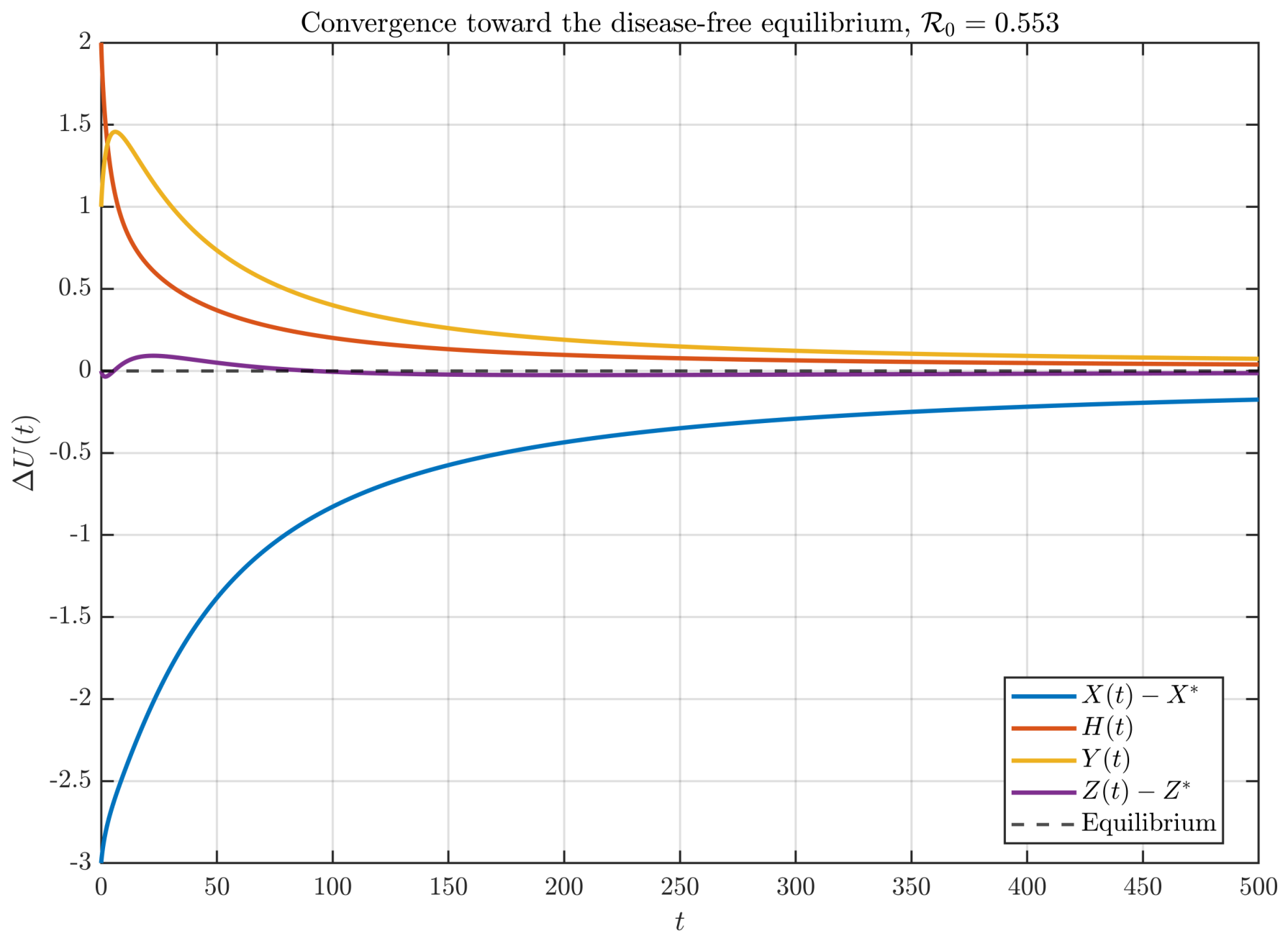
Figure 1 illustrates the transient evolution of the deviations from the disease-free equilibrium over $0\le t\le 500$. The susceptible and immune deviations decrease, while the exposed and infectious populations exhibit an overall decay after a short initial increase in $Y\left(t\right)$, associated with the progression of initially exposed individuals. At the finite terminal time $t=500$,

$$\left|X\left(500\right)-X_0\right|=1.7494\times {10}^{-1},H\left(500\right)=3.8972\times {10}^{-2},$$

$$Y\left(500\right)=7.3532\times {10}^{-2},\left|Z\left(500\right)-Z_0\right|=1.3892\times {10}^{-2}.$$

Moreover,

$$H\left(500\right)+Y\left(500\right)=1.1250\times {10}^{-1},$$

which is approximately $3.75\%$ of its initial value $H\left(0\right)+Y\left(0\right)=3$. The infected components therefore remain nonzero at the finite terminal time $t=500$, but their substantial reduction illustrates convergence toward the disease-free state over the simulated interval. This numerical trajectory is not intended as an independent proof of asymptotic stability; rather, it illustrates behavior consistent with the local asymptotic stability of ${\mathcal{E}}_0$ established analytically in Theorem 4. In particular, asymptotic stability requires convergence to the equilibrium as $t\to \infty$, rather than exact extinction of the infected compartments at a finite simulation time. The relatively slow decay observed over the finite time interval also illustrates the persistent transient effects associated with distributed-order memory.

5.2. Dynamics of the Endemic Equilibrium

To examine endemic dynamics, the transmission rate is increased to $\beta =0.35$, while all other parameters remain unchanged. This gives ${\mathcal{R}}_0=1.612505>1,$ so the disease-free equilibrium is unstable. A uniform memory distribution is used over $\alpha \in [0.70,1.00]$, with initial condition

$$\left(X\left(0\right),H\left(0\right),Y\left(0\right),Z\left(0\right)\right)=(650,20,10,320),N\left(0\right)=1000.$$

The numerically computed endemic equilibrium is

$${\mathcal{E}}^{\ast }=\left(362.377258,84.479329,131.439986,324.659185\right),$$

with $N^{\ast }=902.955758.$ The residual

$${∥\mathbf{F}\left({\mathcal{E}}^{\ast }\right)∥}_{\infty }=2.8237\times {10}^{-10}$$

confirms that the computed state satisfies the equilibrium equations to high numerical accuracy.

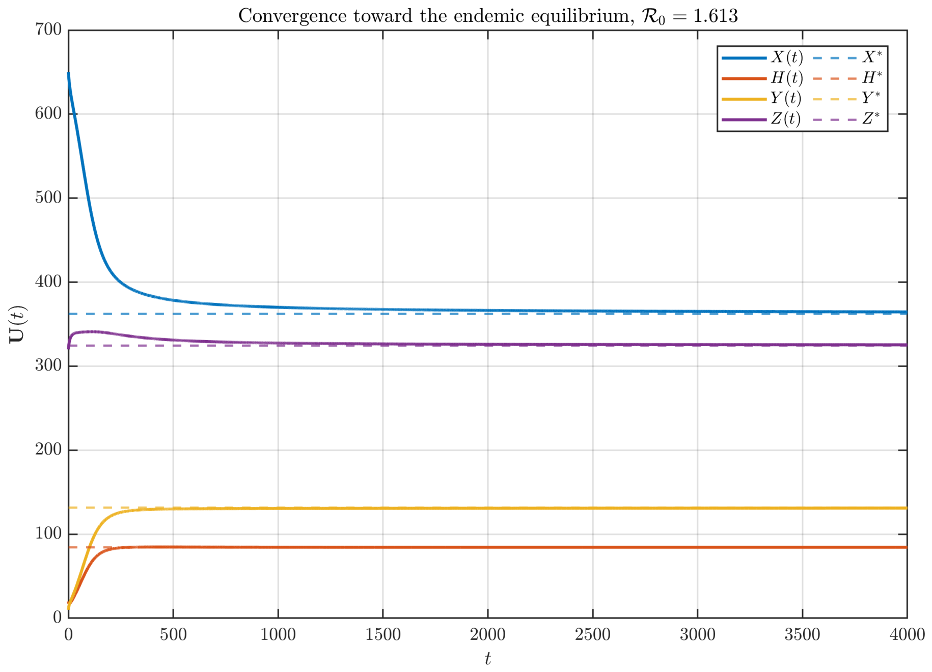
Figure 2 shows the compartment trajectories over $0\le t\le 4000$. The susceptible population decreases toward $X^{\ast }$, whereas the exposed and infectious populations approach the positive levels $H^{\ast }$ and $Y^{\ast }$. The immune population also converges toward $Z^{\ast }$. At $T=4000$,

$$\begin{array}{cccc}\hfill X\left(T\right)& =364.582232,\hfill & \hfill H\left(T\right)& =84.451201,\hfill \\ \hfill Y\left(T\right)& =131.113359,\hfill & \hfill Z\left(T\right)& =325.379465.\hfill \end{array}$$

The corresponding relative errors are approximately

$$0.6085\%,0.0333\%,0.2485\%,0.2219\%,$$

respectively. Thus, all components are within $0.61\%$ of their endemic equilibrium values. These results provide numerical evidence that the endemic equilibrium is locally attracting for the selected parameter set. The persistent positive values of $H\left(t\right)$ and $Y\left(t\right)$ indicate endemic infection, while the slow long-time convergence reflects the transient memory effects generated by the distributed-order fractional derivative.

5.3. Influence of Distributed-Order Memory on Endemic Stability

This experiment investigates whether distributed-order memory can induce an oscillatory stability transition at the endemic equilibrium. A uniform memory distribution is considered on

$$\alpha \in [0.70,1],$$

so that

$${\Psi }_{\omega }\left(s\right)={\int }_{0.70}^1\omega \left(\alpha \right)T_c^{\alpha -1}{s}^{\alpha }d\alpha ,\omega \left(\alpha \right)={\displaystyle \frac{1}{0.30}},$$

and the characteristic equation is

$$det\left({\Psi }_{\omega }\left(s\right)I-J\right)=0,$$

where J is the Jacobian matrix evaluated at the endemic equilibrium.

The baseline parameters are

$$r=0.02,q=0.40,p=0.05,\epsilon =0.10,\sigma =0.20,\gamma =0.10,\mu =0.01,\beta =0.35,$$

with

$$f\left(N\right)=d_0+cN,d_0=0.005,c={\displaystyle \frac{r-d_0}{K}},K=1000.$$

These values yield ${\mathcal{R}}_0=1.612505>1,$ and the endemic equilibrium

$$E^{\ast }=(362.377258,84.479329,131.439986,324.659185),$$

with $N^{\ast }=902.955757.$ The equilibrium residual,

$$\parallel F\left(E^{\ast }\right){\parallel }_{\infty }=7.1054\times {10}^{-15},$$

confirms the numerical accuracy of the computed steady state. The distributed-order characteristic symbol was evaluated using a 16-point Gauss–Legendre quadrature over $[0.70,1]$. Its real and imaginary parts satisfy

$$3.026741\times {10}^{-5}\le Re{\Psi }_{\omega }\left(i\nu \right)\le 1.481999,$$

and

$$8.281248\times {10}^{-5}\le Im{\Psi }_{\omega }\left(i\nu \right)\le 7.000846,$$

indicating that the spectral curve remains entirely within the first quadrant. The stability switching analysis developed above provides a systematic criterion for detecting an oscillatory loss of stability through the condition

$${\Psi }_{\omega }\left(i\nu \right)={\lambda }_j\left(J\right),\nu >0.$$

In particular, a stability switch requires a characteristic root to reach the imaginary axis and satisfy the transversality condition of Theorem 8. In the numerical experiments reported below, the emphasis is therefore placed on fully reproducible parameter sets and memory configurations for which all model parameters, initial conditions, and numerical settings are explicitly specified. The simulations show that distributed-order memory can substantially modify the rate of transient decay and the persistence of perturbations. However, the numerical experiments presented here should not be interpreted as an exhaustive exclusion of oscillatory stability transitions over the full biologically admissible parameter space.

5.4. Influence of the Memory Interval on Endemic Transients

To investigate the influence of distributed-order memory on the transient dynamics of the endemic equilibrium, the epidemiological parameters and initial perturbation were fixed as in the previous subsection. Four uniform distributed-order densities with supports

$$[0.95,1],[0.80,1],[0.60,1],[0.40,1]$$

were considered. Consequently, any differences in the numerical solutions arise solely from the choice of the memory interval.

The simulations were performed over $0\le t\le 1000,$ using a time step of $\Delta t=0.5$. The transient response was quantified by the normalized perturbation

$$D\left(t\right)={\displaystyle \frac{\parallel \mathbf{U}\left(t\right)-E^{\ast }{\parallel }_2}{\parallel \mathbf{U}\left(0\right)-E^{\ast }{\parallel }_2}},$$

the settling time defined by

$$D\left(t\right)\le {10}^{-2},$$

and the accumulated perturbation

$$\mathcal{P}={\int }_0^{1000}D\left(t\right)dt.$$

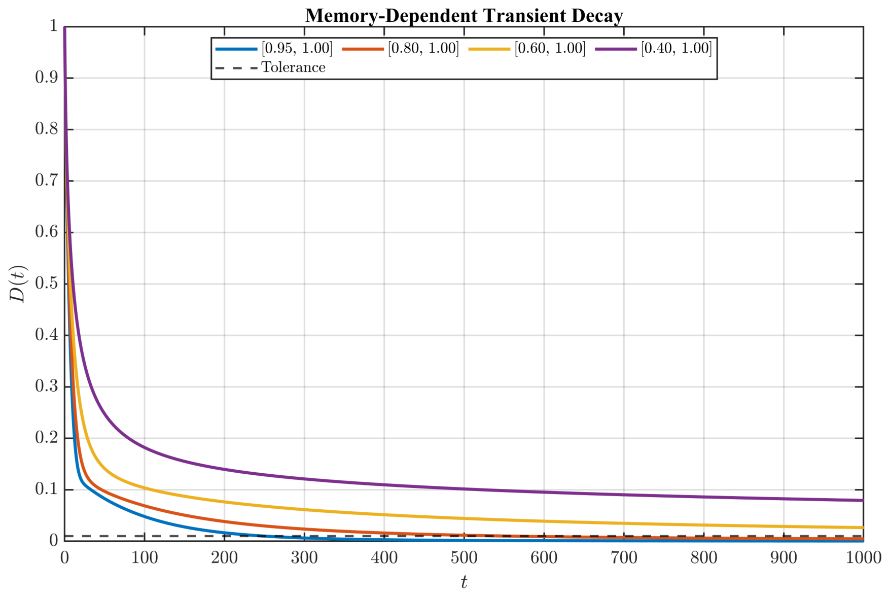
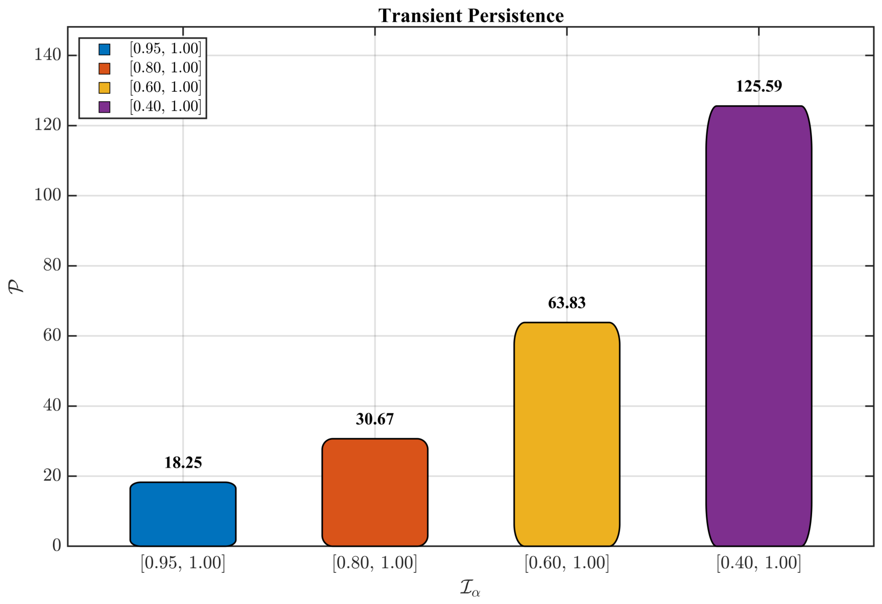
The corresponding indicators are summarized in

Table 2. Transient indicators for different distributed-order memory densities on the fixed support $[0.40,1]$.

Density	Mean Order	D (1000)	$\mathcal{P}$	Half-Decay Time	Quarter-Decay Time
Uniform	$0.70$	$7.932365\times {10}^{-2}$	$125.587906$	$10.5$	$49.0$
Increasing	$0.80$	$3.680295\times {10}^{-2}$	$74.101701$	$7.5$	$23.0$
Decreasing	$0.60$	$1.097285\times {10}^{-1}$	$167.523913$	$16.0$	$99.5$
Beta-type	$0.70$	$6.434691\times {10}^{-2}$	$109.286766$	$10.0$	$41.0$

. Figure 3 shows the evolution of the normalized perturbation for the four memory intervals. In all cases, $D\left(t\right)$ decreases monotonically, indicating behavior consistent with the asymptotic stability of the endemic equilibrium. However, the convergence rate depends strongly on the support of the memory distribution. The interval $[0.95,1]$ exhibits the fastest relaxation, reaching the prescribed settling tolerance after approximately 250 time units. Expanding the support to $[0.80,1]$ delays convergence to approximately $557.5$, whereas for the broader intervals $[0.60,1]$ and $[0.40,1]$ the perturbation remains above the tolerance throughout the simulation. The cumulative effect of the memory interval is illustrated in Figure 4. The accumulated perturbation increases monotonically from $18.2536$ for $[0.95,1]$ to $125.5879$ for $[0.40,1]$. Likewise, the final relative perturbation increases from $4.8613\times {10}^{-4}$ to $7.9324\times {10}^{-2},$ showing that progressively broader memory intervals produce substantially longer transient responses. The maximum infectious deviation,

$$max|Y-Y^{\ast }|=2.6288,$$

is identical for all simulations because the same initial perturbation is employed. Overall, broadening the distributed-order interval toward lower fractional orders weakens transient damping, delays convergence, and increases the cumulative perturbation. Nevertheless, all trajectories remain bounded and converge to the same endemic equilibrium, indicating that the memory interval affects the transient dynamics without altering the asymptotic stability of the endemic equilibrium.

5.5. Effect of the Memory Density Shape on Endemic Transients

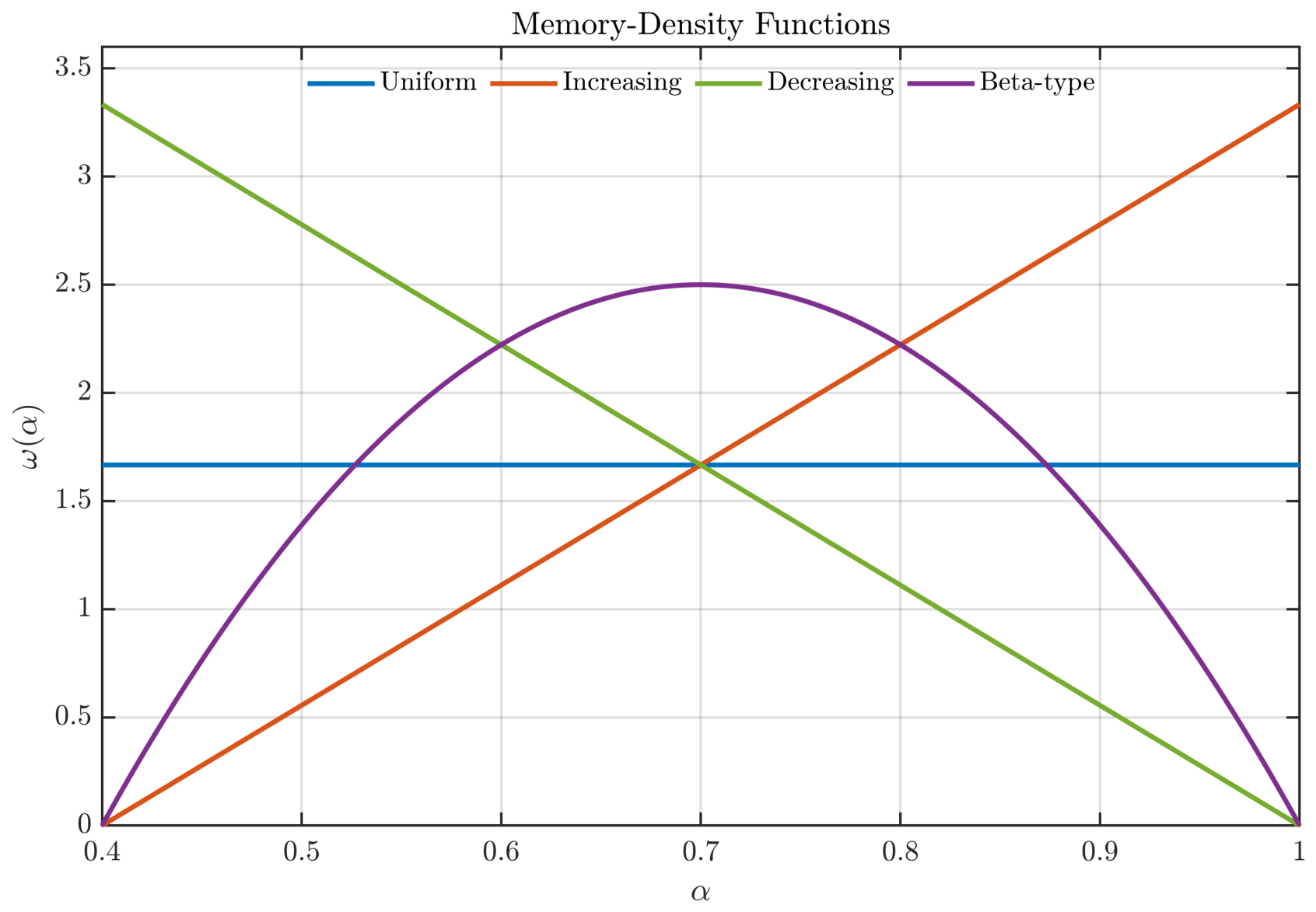
The previous experiment showed that broadening the support of the distributed-order derivative toward lower fractional orders increases transient persistence. We now investigate the influence of the shape of the memory density while keeping its support fixed at $\alpha \in [0.40,1].$ Four normalized memory densities were considered:

$${\omega }_1\left(\alpha \right)={\displaystyle \frac{1}{0.60}},$$

$${\omega }_2\left(\alpha \right)={\displaystyle \frac{2(\alpha -0.40)}{{\left(0.60\right)}^2}},$$

$${\omega }_3\left(\alpha \right)={\displaystyle \frac{2(1-\alpha )}{{\left(0.60\right)}^2}},$$

and

$${\omega }_4\left(\alpha \right)={\displaystyle \frac{6\xi (1-\xi )}{0.60}},\xi ={\displaystyle \frac{\alpha -0.40}{0.60}},$$

representing the uniform, increasing, decreasing, and symmetric beta-type densities, respectively. Their profiles are shown in Figure 5.

The corresponding weighted mean fractional orders are

$${\overline{\alpha }}_1=0.70,{\overline{\alpha }}_2=0.80,{\overline{\alpha }}_3=0.60,{\overline{\alpha }}_4=0.70,$$

with variances $0.030$, $0.020$, $0.020$, and $0.018$, respectively. Thus, the increasing density emphasizes higher fractional orders, whereas the decreasing density assigns greater weight to lower orders. The uniform and beta-type densities have the same weighted mean order but different distributions of memory weight. The epidemiological parameters, endemic equilibrium, and initial perturbation were identical to those used in the previous experiment. The simulations were carried out over $0\le t\le 1000,$ using $\Delta t=0.5$ and a 20-point Gauss–Legendre quadrature for the distributed-order approximation. The transient response was quantified by the normalized perturbation

$$D\left(t\right)={\displaystyle \frac{\parallel U\left(t\right)-E^{\ast }{\parallel }_2}{\parallel U\left(0\right)-E^{\ast }{\parallel }_2}},$$

the accumulated perturbation

$$\mathcal{P}={\int }_0^{1000}D\left(t\right)dt,$$

and the times required for the perturbation to decay to one-half and one-quarter of its initial magnitude.

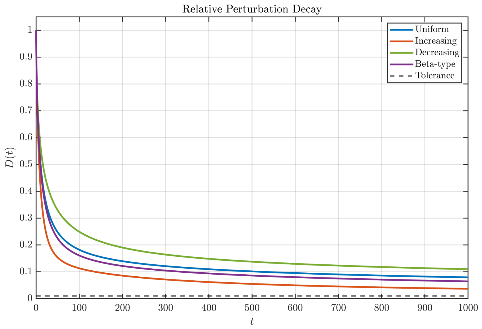
Figure 6 shows the evolution of the normalized perturbation. All four trajectories converge to the same endemic equilibrium, confirming that the equilibrium is independent of the memory density shape. Nevertheless, the convergence rate depends strongly on the distribution of memory weight. The increasing density exhibits the fastest relaxation, with

$$D\left(1000\right)=3.680295\times {10}^{-2},\mathcal{P}=74.101701,$$

whereas the decreasing density produces the slowest decay,

$$D\left(1000\right)=1.097285\times {10}^{-1},\mathcal{P}=167.523913.$$

The uniform and beta-type densities yield intermediate responses. Although these two densities have the same weighted mean order $\overline{\alpha }=0.70$, the beta-type density produces smaller values of both $D\left(1000\right)$ and $\mathcal{P}$, demonstrating that the mean fractional order alone does not determine the transient dynamics. The distribution of memory weight across the support also plays a significant role. Overall, the transient persistence follows the ordering

$$\mathrm{Increasing}<\mathrm{Beta}\text{-}\mathrm{type}<\mathrm{Uniform}<\mathrm{Decreasing}.$$

Hence, concentrating the memory density near lower fractional orders substantially weakens transient damping, whereas emphasizing higher fractional orders accelerates relaxation. In all cases, the perturbation decays monotonically toward the same endemic equilibrium, indicating that the memory density shape influences only the transient dynamics and not the asymptotic stability of the endemic equilibrium.

The numerical parameters used in the above experiments were selected to represent epidemiologically meaningful time scales while also providing parameter regimes suitable for illustrating the threshold and memory-dependent dynamics of the model. In particular, the rates r, $\sigma$, $\gamma$, $\mu$, $\epsilon$, and p represent demographic turnover, progression from latency to infectiousness, recovery, disease-induced mortality, loss of temporary immunity, and booster vaccination, respectively, whereas q represents the fraction successfully vaccinated at birth. The transmission parameter $\beta$ was varied to obtain regimes with ${\mathcal{R}}_0<1$ and ${\mathcal{R}}_0>1$, allowing the disease-free and endemic dynamics to be examined separately. For comparisons involving distributed-order memory, all epidemiological parameters and initial conditions were kept fixed, and only the memory interval or the density $\omega \left(\alpha \right)$ was changed. Thus, the observed differences in transient decay, settling time, and accumulated perturbation can be attributed directly to the distributed-order memory rather than to changes in the underlying epidemiological parameters.

The present results can be compared with several related epidemic models in the literature. Classical integer-order epidemic models have shown that demographic effects, latency, and loss of immunity can substantially influence epidemic thresholds and stability [2]. The fractional SEIR model with density-dependent mortality in [6] introduced memory effects through a single fractional order, whereas the distributed-order hantavirus model in [15] employed a weighted spectrum of fractional orders. The present study extends the distributed-order approach to an SEIRS framework incorporating temporary immunity, vaccination, disease-induced mortality, and density-dependent natural mortality. Related fractional epidemic studies have also investigated global stability in SVEIR and SIRS models [16,18], while the dual-memory fractional SEIR model in [19] demonstrated that multiple memory mechanisms can influence epidemic thresholds and dynamics. In contrast to these formulations, the present analysis systematically examines both the support and shape of the memory distribution $\omega \left(\alpha \right)$. The results show that extending the memory interval toward lower fractional orders slows convergence to the endemic equilibrium, whereas densities concentrated near $\alpha =1$ produce faster relaxation. Moreover, distributions having the same mean fractional order can generate different transient responses, showing that the mean order alone does not fully characterize the memory effect. Finally, Greenhalgh [24] showed that latency and nonpermanent immunity can generate Hopf bifurcation in an integer-order epidemic model. In contrast, the present distributed-order spectral analysis detects no purely imaginary characteristic roots within the investigated parameter ranges. Thus, for the cases considered here, distributed-order memory primarily modifies transient damping and persistence rather than inducing an oscillatory stability transition.

6. Sensitivity Analysis of Distributed-Order Memory

The preceding experiments show that distributed-order memory primarily affects the transient behavior of the epidemic while preserving the endemic equilibrium for the parameter ranges considered.

First, the numerical spectral analysis detected no intersection between the distributed-order spectral curve and an admissible unstable complex mode of the endemic Jacobian. Thus, no purely imaginary characteristic root or memory-induced oscillatory stability transition was observed. Second, broadening the support of a uniform memory density toward lower fractional orders substantially increased transient persistence. As the interval changed from $[0.95,1]$ to $[0.40,1]$, the final relative perturbation increased from

$$4.8613\times {10}^{-4}\mathrm{to}7.9324\times {10}^{-2},$$

while the accumulated perturbation increased from approximately $18.25$ to $125.59$. The intervals $[0.95,1]$ and $[0.80,1]$ reached the prescribed settling tolerance at approximately $t=250$ and $t=557.5$, respectively, whereas the broader intervals did not settle within the simulated time. Finally, the shape of the memory density strongly influenced the transient response even when the support was fixed at $[0.40,1]$. The increasing density, which emphasizes higher fractional orders, produced the fastest relaxation, with

$$D\left(1000\right)=3.680295\times {10}^{-2},\mathcal{P}=74.101701.$$

The decreasing density produced the strongest persistence, with

$$D\left(1000\right)=1.097285\times {10}^{-1},\mathcal{P}=167.523913.$$

The resulting ordering was

$$\mathrm{increasing}<\mathrm{beta}-\mathrm{type}<\mathrm{uniform}<\mathrm{decreasing}.$$

The different responses obtained for the uniform and beta-type densities, despite their common mean order $\overline{\alpha }=0.70$, show that the mean fractional order alone does not determine transient behavior. The distribution of memory weight across the fractional-order interval is also important. Overall, greater emphasis on lower fractional orders weakens transient damping and prolongs epidemic memory, whereas concentration near the classical order accelerates convergence. Within the investigated parameter ranges, all solutions remained bounded and approached the same endemic equilibrium, with no evidence of an oscillatory stability transition.

7. Conclusions

In this paper, a distributed-order fractional SEIRS epidemic model with vaccination, temporary immunity, disease-induced mortality, and density-dependent natural mortality was investigated. The basic reproduction number and equilibria were derived, and their local stability properties were analyzed through the distributed-order characteristic equation. In addition, a sufficient global disease extinction criterion was established using a distributed-order Lyapunov argument, providing conditions for global asymptotic stability of the disease-free equilibrium. For the parameter ranges considered, the numerical spectral analysis detected no oscillatory stability transition. The simulations showed that distributed-order memory mainly controls transient epidemic behavior. Extending the memory interval toward lower fractional orders slowed convergence and increased transient persistence, while changing the memory density shape altered the damping rate even when the support was fixed. Densities concentrated near lower orders produced the strongest persistence, whereas those weighted toward the classical order gave the fastest relaxation. Thus, both the support and shape of the memory distribution influence endemic transients without changing the long-term equilibrium observed in the simulations. Future research will focus on estimating the memory distribution and epidemiological parameters from real data, developing optimal intervention strategies, and extending the framework to spatially heterogeneous and stochastic epidemic models. Establishing global stability of the endemic equilibrium for general population-dependent contact rates and extending the analysis to more general memory kernels remain important directions for future research.

References

1. Hethcote, H.W. The mathematics of infectious diseases. SIAM Rev. 2000, 42, 599–653. [Google Scholar] [CrossRef] [Scilit]
2. Greenhalgh, D. Some threshold and stability results for epidemic models with a density-dependent death rate. Theor. Popul. Biol. 1992, 42, 130–151. [Google Scholar] [CrossRef] [Scilit]
3. Chen-Charpentier, B. SIRS epidemic models with delays, partial and temporary immunity and vaccination. AppliedMath 2024, 4, 666–689. [Google Scholar] [CrossRef] [Scilit]
4. Angelov, G.; Kovacevic, R.; Stilianakis, N.I.; Veliov, V.M. An immuno-epidemiological model with waning immunity after infection or vaccination. J. Math. Biol. 2024, 88, 71. [Google Scholar] [CrossRef] [Scilit]
5. Al-Arydah, M. Assessing vaccine efficacy for infectious diseases with variable immunity using a mathematical model. Sci. Rep. 2024, 14, 18572. [Google Scholar] [CrossRef] [Scilit]
6. Demirci, E.; Unal, A.; Ozalp, N. A fractional order SEIR model with density dependent death rate. Hacet. J. Math. Stat. 2011, 40, 287–295. [Google Scholar]
7. Chen, Y.; Liu, F.; Yu, Q.; Li, T. Review of fractional epidemic models. Appl. Math. Model. 2021, 97, 281–307. [Google Scholar] [CrossRef] [Scilit]
8. Barros, L.C.; Lopes, M.M.; Pedro, F.S.; Esmi, E.; Santos, J.P.C.; Sánchez, D.E. The memory effect on fractional calculus: An application in the spread of COVID-19. Comput. Appl. Math. 2021, 40, 72. [Google Scholar] [CrossRef] [Scilit]
9. Nisar, K.S.; Farman, M.; Abdel-Aty, M.; Ravichandran, C. A review of fractional order epidemic models for life sciences problems: Past, present and future. Alex. Eng. J. 2024, 95, 283–305. [Google Scholar] [CrossRef] [Scilit]
10. DarAssi, M.H.; Safi, M.A.; Khan, M.A.; Beigi, A.; Aly, A.A.; Alshahrani, M.Y. A mathematical model for SARS-CoV-2 in variable-order fractional derivative. Eur. Phys. J. Spec. Top. 2022, 231, 1905–1914. [Google Scholar] [CrossRef] [Scilit]
11. Jiao, Z.; Chen, Y.Q.; Podlubny, I. Distributed-Order Dynamic Systems: Stability, Simulation, Applications and Perspectives; Springer: London, UK, 2012. [Google Scholar] [CrossRef] [Scilit]
12. Najafi, H.S.; Sheikhani, A.R.; Ansari, A. Stability analysis of distributed order fractional differential equations. Abstr. Appl. Anal. 2011, 2011, 175323. [Google Scholar] [CrossRef] [Scilit]
13. Jiao, Z.; Chen, Y.Q.; Zhong, Y. Stability analysis of linear time-invariant distributed-order systems. Asian J. Control 2013, 15, 640–647. [Google Scholar] [CrossRef] [Scilit]
14. Diethelm, K.; Ford, N.J. Numerical analysis for distributed-order differential equations. J. Comput. Appl. Math. 2009, 225, 96–104. [Google Scholar] [CrossRef] [Scilit]
15. Kocabiyik, M.; Ongun, M.Y. Distributed order hantavirus model and its nonstandard discretizations and stability analysis. Math. Meth. Appl. Sci. 2025, 48, 2404–2420. [Google Scholar] [CrossRef] [Scilit]
16. Nabti, A.; Ghanbari, B. Global stability analysis of a fractional SVEIR epidemic model. Math. Meth. Appl. Sci. 2021, 44, 8577–8597. [Google Scholar] [CrossRef] [Scilit]
17. Barbarossa, M.V.; Polner, M.; Röst, G. Stability switches induced by immune system boosting in an SIRS model with discrete and distributed delays. SIAM J. Appl. Math. 2017, 77, 905–923. [Google Scholar] [CrossRef] [Scilit]
18. Wu, Z.; Cai, Y.; Wang, Z.; He, D.; Wang, W. Global dynamics of a fractional order SIRS epidemic model by the way of generalized continuous time random walk. J. Math. Biol. 2025, 90, 39. [Google Scholar] [CrossRef] [Scilit]
19. Wu, Z.; Cai, Y.; Wang, Z.; Tan, Y.; He, D.; Wang, W. Dual memory effects and epidemic thresholds in a fractional-order SEIR model. Appl. Math. Comput. 2026, 524, 130037. [Google Scholar] [CrossRef] [Scilit]
20. Zinihi, A.; Ehrhardt, M.; Ammi, M.R.S. Spatiotemporal SEIQR epidemic modeling with optimal control for vaccination, treatment, and social measures. J. Math. Biol. 2026, 93, 10. [Google Scholar] [CrossRef] [Scilit]
21. Jajarmi, A. Generalized fractional modeling and optimal control of respiratory syncytial virus infections in Florida. Sci. Rep. 2026, 16, 9728. [Google Scholar] [CrossRef] [Scilit]
22. Mbare, N.S. Fractional-order analysis of asymptomatic COVID-19 transmission dynamics with stability and control strategies. Discov. Public Health 2026, 23, 72. [Google Scholar] [CrossRef] [Scilit]
23. Chauhan, J.P.; Jebran, S.; Khirsariya, S.R. Stability analysis and numerical investigation of fractional SIR model for childhood disease transmission with vaccination. Sci. Rep. 2026, 16, 23605. [Google Scholar] [CrossRef] [Scilit]
24. Greenhalgh, D. Hopf bifurcation in epidemic models with a latent period and nonpermanent immunity. Math. Comput. Model. 1997, 25, 85–107. [Google Scholar] [CrossRef] [Scilit]
25. Xiao, J.; Shi, K.; Teng, Y.; Qi, J.; Fan, H. Relaxed research on synchronization problem of fractional-order fuzzy octonion-valued BAM neural networks by the non-decomposition method on the high-dimension oblique field. Fractal Fract. 2026, 10, 414. [Google Scholar] [CrossRef] [Scilit]
26. Ding, W.; Patnaik, S.; Sidhardh, S.; Semperlotti, F. Applications of Distributed-Order Fractional Operators: A Review. Entropy 2021, 23, 110. [Google Scholar] [CrossRef] [Scilit]
27. Caputo, M.; Fabrizio, M. A new definition of fractional derivative without singular kernel. Prog. Fract. Differ. Appl. 2015, 1, 73–85. [Google Scholar]
28. Atangana, A.; Baleanu, D. New fractional derivatives with nonlocal and non-singular kernel: Theory and application to heat transfer model. Therm. Sci. 2016, 20, 763–769. [Google Scholar] [CrossRef] [Scilit]
29. Luchko, Y. Maximum principle and its application for the time-fractional diffusion equations. Fract. Calc. Appl. Anal. 2011, 14, 110–124. [Google Scholar] [CrossRef] [Scilit]
30. Aminikhah, H.; Sheikhani, A.R.; Rezazadeh, H. Stability Analysis of Distributed Order Fractional Chen System. Sci. World J. 2013, 2013, 645080. [Google Scholar] [CrossRef] [Scilit]
Figure 1. Convergence to the disease-free equilibrium for R 0 = 0.552859 < 1 . The curves represent X ( t ) X 0 , H ( t ) , Y ( t ) , and Z ( t ) Z 0 ; the dashed line indicates the equilibrium level.
Mathematics 14 03186 g001
Figure 2. Convergence to the endemic equilibrium for R 0 = 1.612505 > 1 . Solid curves represent the numerical solutions, and dashed lines indicate the equilibrium values X , H , Y , and Z .
Mathematics 14 03186 g002
Figure 3. Relative perturbation norm for different distributed-order memory intervals. Broader intervals containing lower fractional orders exhibit slower transient decay and longer relaxation times. The dashed line denotes the settling tolerance.
Mathematics 14 03186 g003
Figure 4. Accumulated transient perturbation for different distributed-order memory intervals. Broader intervals containing lower fractional orders increase transient persistence while preserving asymptotic stability.
Mathematics 14 03186 g004
Figure 5. Normalized distributed-order memory density functions on the fixed support [ 0.40 , 1 ] : uniform, increasing, decreasing, and beta-type densities.
Mathematics 14 03186 g005
Figure 6. Relative perturbation from the endemic equilibrium for the four memory density functions. The increasing density produces the fastest decay, whereas the decreasing density yields the strongest transient persistence.
Mathematics 14 03186 g006