A Convex-Dependent NHPP Software Reliability Model and Its Deep-Learning-Based Parameter Estimation

Abstract

Many software systems currently under development exhibit numerous new types of failure due to their structural complexity. This suggests the need for research on structures capable of representing convex patterns in the fault-detection rate over time. This paper proposes a non-homogeneous Poisson process (NHPP) software reliability model (SRM) incorporating a convex fault-detection rate. To validate this, we compared 13 SRMs with different forms using three datasets to evaluate the effectiveness and applicability of the proposed model. Furthermore, the performance of the proposed model was evaluated through comparisons with multiple models, and a deep-learning-based parameter estimation (DL-BPE) was introduced as an alternative estimation framework. The proposed DL-BPE provides a competitive and flexible parameter estimation framework, showing improved predictive performance in several datasets while preserving the structural interpretability of the proposed NHPP SRM. Based on the results, we propose new assumptions for enhancing the reliability of increasingly complex software packages. The DL-BPE framework may provide a basis for integrating interpretable reliability-model structures into deep-learning architectures for software reliability analysis.

1. Introduction

Software has significantly enhanced the quality of human life over time by performing diverse roles across various fields. The emergence of open-source software has driven diversification in the software market, expanding and evolving via contributions from non-experts who wish to utilize it. Artificial intelligence (AI)-based software has elevated the quality of human life to a new dimension, advancing human capabilities in thinking, productivity, and diversity through generative AI software.

As software occupies a crucial part of our lives, it has developed an inseparable relationship with humanity. At this very moment, when the importance of software is increasing, if a defect or error occurs in even a small part of the software or an unknown failure occurs in the entire system, it is expected to cause immense economic damage, including social problems and the costs incurred to solve them, during the period when the system stops or malfunctions.

On 19 July 2024, an update containing faults was released for the Falcon Sensor security software distributed by the U.S. cybersecurity firm CrowdStrike. This caused large-scale computer failures, affecting approximately 8.5 million computers, resulting in boot failures and blue screen errors. The incident impacted various industries, with direct losses for Fortune 500 companies estimated at approximately $5.4 billion. This case was identified as being caused by an internal software update fault, serving as an example illustrating the risks of relying on centralized security solutions [1].

Such software failures and faults arise from various causes, including coding errors and compatibility issues, making their control important. Furthermore, because software users rely on them functioning without errors, ensuring a sufficient level of reliability is of paramount concern. Research on software reliability models (SRMs) that predict failures continues to advance in order to enhance software reliability.

Research to enhance software reliability has resulted in the development of diverse methodologies. These approaches are widely used in various methodologies, including time-series models that reflect the characteristics of failure data and curve-fitting models that describe the relationship between independent and dependent variables [2,3,4,5]. In particular, research on SRMs assuming a non-homogeneous Poisson process (NHPP), in which failures occur differently over time, has been actively conducted.

The NHPP SRM proposed by Goel and Okumoto in 1979 has since been extended under various assumptions [6]. Research has been conducted under various assumptions, including incomplete debugging where faults are not fully corrected, testing efforts expended to correct faults, the occurrence of dependent faults where one software fault affects others, and uncertain operating environments, assuming differences between the testing and actual environment [7,8,9,10]. Furthermore, these models have been extended to non-parametric methods. Unlike previously proposed parametric methods, this approach does not rely on assumptions regarding the occurrence of software faults or failures. Instead, it proposes an SRM that predicts software faults using information about defects that have actually occurred. This method offers greater flexibility than parametric methods and provides more accurate results [11,12,13].

In particular, among non-parametric methods, deep learning approaches have been utilized in various structural forms as one of several methods to enhance software reliability. The most fundamental deep neural network was proposed as an ensemble model comprising multiple neural network structures, contributing to improved software reliability through multiple models rather than a single model. Furthermore, the deep neural network structure was extended to develop a framework capable of estimating the parameters for previously developed SRMs [14]. In another study, a model was developed, which utilized a testing effort function rather than relying solely on time, employing a structure in which testing intensity varies over time. Alternatively, an SRM can be structured as a minimal composite function, alongside a structure in which each function possesses a hidden layer [15,16,17].

In addition, research on improving software reliability using deep neural networks has involved the application of deep learning for direct model development, for selecting the optimal model from developed SRMs, or for identifying and improving the numerous defects occurring in open-source software [18,19].

The data used to develop SRMs exhibit sequential characteristics. Therefore, an SRM for enhancing software reliability has been developed using a recurrent neural network (RNN) architecture that reflects these sequential properties. The RNN studied here is not a traditional RNN architecture, but a modified RNN structure designed to reflect the SRM’s structure, enabling learning at subsequent time steps [20]. This was extended to develop an ensemble model capable of simultaneously incorporating multiple SRMs [21].

Additionally, studies utilizing encoder–decoder architectures have also been conducted [22]. Using RNNs suitable for sequential data characteristics, models utilizing seq2seq structures or attention-based models were employed to predict the next time step and endpoints, or to enhance the performance for small-scale data prediction. A method was also proposed to address the issue of small-scale data inherent in software failure data by applying dropout [23,24]. A recent study in the broader reliability field compared machine-learning methods for estimating binary-state network reliability under varying levels of data availability [25].

This paper proposes an NHPP SRM with a convex fault-detection rate and a nonzero initial failure state. This study evaluates the proposed model by comparing it with several existing SRMs. Furthermore, in addition to the least-squares estimation (LSE) and maximum likelihood estimation (MLE), this study introduces a deep-learning-based parameter estimation (DL-BPE) framework that incorporates the proposed SRM structure into an RNN. Section 2 introduces the proposed convex shape. Section 3 introduces the parameter estimation methods and the newly proposed DL-BPE method. Section 4 evaluates the proposed model and the DL-BPE framework through numerical examples. Section 5 discusses the findings and limitations, and Section 6 concludes the study.

2. Software Reliability Model

In this study, we propose an NHPP SRM that incorporates a convex fault-detection rate and dependent failures to represent complex software failure processes. This Section presents the mathematical framework required to formulate the proposed model. First, the Weibull-based fault-detection rate is introduced, and the parameter conditions under which it exhibits convex behavior are examined. Based on this formulation, the dependent-failure mechanism is incorporated into the NHPP differential equation, and the resulting mean value function is derived under a nonzero initial condition.

2.1. NHPP SRM

Software reliability refers to the ability of software to function properly without failures or defects and is evaluated to assess the reliability of the software. SRMs have been studied to enhance reliability. Among the numerous reliability research methodologies, those assuming an NHPP have been actively conducted. The NHPP is defined as a Poisson process where the occurrence of failures and faults follows a mean-value function $m\left(t\right)$ whose parameters vary over time, rather than a Poisson distribution with a parameter $\lambda$. This follows from Equation (1):

$$\mathrm{Pr}\{N\left(t\right)=n\}={\displaystyle \frac{\{{m\left(t\right)\}}^n}{n!}}{e}^{-m\left(t\right)},n=\mathrm{0,1},2,\cdots ,t\ge 0$$

(1)

where $m\left(t\right)$ represents the mean value function from time $0$ to $t$. The mean value function $m\left(t\right)$ is fundamentally derived from differential Equation (2), which calculates the difference between the total number of failures $a\left(t\right)$ and the mean value function $m\left(t\right)$ at time $t$, multiplied by the fault-detection rate $b\left(t\right)$ at that time. Rearranging this yields the general form shown in Equation (3) [5].

$${\displaystyle \frac{dm\left(t\right)}{dt}}=b\left(t\right)·[a\left(t\right)-m(t)]$$

(2)

$$m(t)=a·\left(1-exp\left(-{\int }_0^{t}b\left(s\right)ds\right)\right)$$

(3)

In 1979, Goel and Okumoto [6] proposed the NHPP SRM from Equation (3) for the cases where $a\left(t\right)=a$ and $b\left(t\right)=b$.

$$m\left(t\right)=a·\left(1-\mathrm{e}\mathrm{x}\mathrm{p}\left(-bt\right)\right)$$

This approach has been extended to the development of many SRMs using various forms of $a\left(t\right)$ and $b\left(t\right)$. In particular, the fault-detection rates of complex software systems may exhibit nonlinear temporal pat-terns. This suggests the need for NHPP SRMs that can represent different curvature patterns in the fault-detection rate over time. To formulate the fault-detection rate $b\left(t\right)$, we use the hazard function derived from the Weibull distribution in Equation (4) [26].

$$b(t)={\displaystyle \frac{f\left(t\right)}{1-F\left(t\right)}}$$

(4)

In this study, the convexity assumption applies specifically to the fault-detection rate $b\left(t\right)$, rather than to the mean value function $m\left(t\right)$. The Weibull hazard function provides a flexible and parsimonious way to represent nonlinear and convex patterns through its shape parameter $\alpha$. Such flexibility is useful for complex software systems, in which the fault-detection process may change nonlinearly over time owing to heterogeneous failures and interactions among software components. In particular, this study focuses on the convex regions of the Weibull hazard function; therefore, $\alpha$ is restricted to $0<\alpha <1$ or $\alpha >2$, while the range $1\le \alpha \le 2$ is excluded.

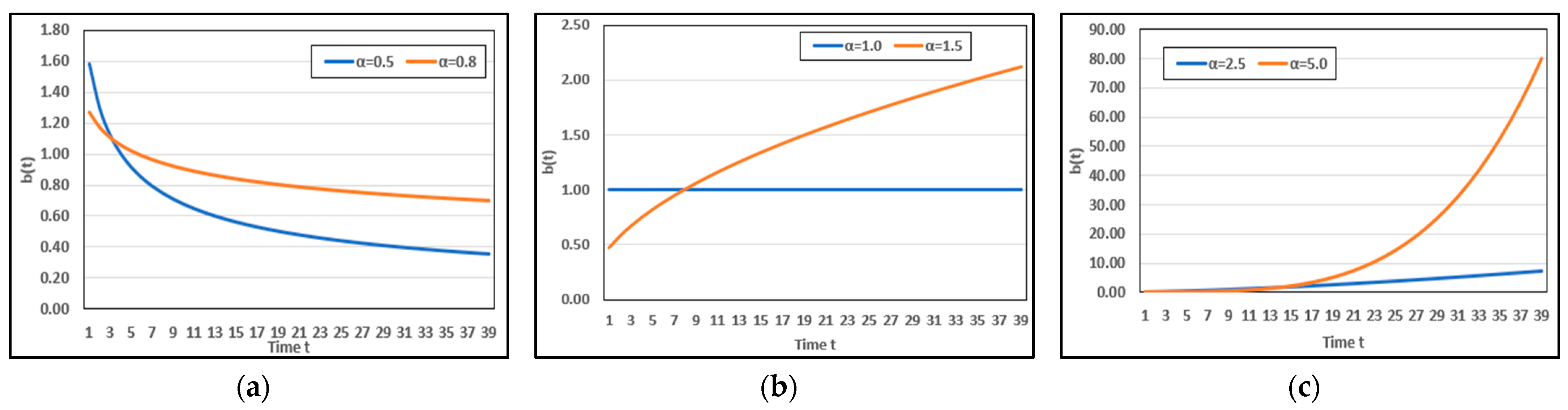
Using the Weibull hazard function in Equation (4), the fault-detection rate function $b\left(t\right)$ is defined as $b\left(t\right)=\alpha {\beta }^{\alpha }{t}^{\alpha -1}(\alpha ,\beta >0)$. Thus, for $t>0$, $b\left(t\right)$ is convex when $0<\alpha <1$, $\alpha >2$. In particular, $b\left(t\right)$ is decreasing and convex when $0<\alpha <1$, whereas it is increasing and convex when $\alpha >2$. The shape parameter $\alpha$ determines the curvature of $b\left(t\right)$, whereas $\beta$ changes its magnitude without altering its curvature for a fixed value of $\alpha$. Figure 1 illustrates the changes in $b\left(t\right)$ for different values of $\alpha$.

Figure 1. Changes in the Weibull-based fault-detection rate $b\left(t\right)$ with $\alpha$; (a) $0<\alpha <1$; (b) $1\le \alpha \le 2$; (c) $\alpha >2.$

The cumulative fault-detection rate is obtained by integrating $b\left(t\right)$ over $0$ to $t$, as shown in Equation (5).

$${\int }_0^{t}b\left(s\right)ds={\int }_0^t\alpha ·{\beta }^{\alpha }·s^{\alpha -1}ds=\alpha ·{\beta }^{\alpha }·{\displaystyle \frac{t^{\alpha }}{\alpha }}={\beta }^{\alpha }·t^{\alpha }$$

(5)

By substituting Equation (5) into Equation (3) and assuming $m\left(0\right)=0$ (no initial failures), the following SRM equation is derived:

$$m\left(t\right)=a\left(1-\mathrm{e}\mathrm{x}\mathrm{p}\left(-{\beta }^{\alpha }{t}^{\alpha }\right)\right)$$

2.2. Proposed NHPP SRM

As software structures become increasingly complex and roles performed by software diversify, software architecture has become highly intricate. In particular, when multiple software components are integrated into a single system, one software component often influences the other. To describe dependent failures in complex software systems, we assume that the expected total failure function is constant over time, $a\left(t\right)=a$. Under this assumption, Equation (6) is formulated by multiplying the right-hand side of Equation (2) by the mean value function $m\left(t\right)$, representing a dependent failure process in which the detection of one failure may be associated with the detection of other failures [9].

$${\displaystyle \frac{dm\left(t\right)}{dt}}=b\left(t\right)·[a-m(t)]·m(t)$$

(6)

Since $m\left(0\right)=0$ yields $m\left(t\right)=0$, we consider a nonzero initial condition $m\left(0\right)>0$. After rearranging Equation (6), integrating both sides, and rearranging with respect to $m\left(t\right)$, we obtain Equation (7).

$$\begin{array}{c}{\displaystyle \frac{1}{\left[a-m\left(t\right)\right]·m\left(t\right)}}dm(t)=b(t)dt\\ \int {\displaystyle \frac{1}{\left[a-m\left(t\right)\right]·m\left(t\right)}}dm\left(t\right)={\displaystyle \frac{1}{a}}\mathrm{l}\mathrm{n}\left|{\displaystyle \frac{m\left(t\right)}{a-m\left(t\right)}}\right|=\int b\left(s\right)ds+C_0\end{array}$$

Since $0<m\left(t\right)<a$, the absolute-value signs can be omitted. Exponentiating both sides and defining $C=exp\left(a{C}_0\right)$ we obtain

$${\displaystyle \frac{m\left(t\right)}{a-m\left(t\right)}}=C·exp\left(a\int b\left(s\right)ds\right).$$

Multiplying both sides by $a-m\left(t\right)$ and collecting the terms involving $m\left(t\right)$ yields

$$m\left(t\right)\left(1+C·exp\left(a\int b\left(s\right)ds\right)\right)=aC·exp\left(a\int b\left(s\right)ds\right).$$

$$m(t)={\displaystyle \frac{a·exp\left(a·\int b\left(s\right)ds\right)·C}{1+exp\left(a·\int b\left(s\right)ds\right)·C}}$$

(7)

Here, $C$ is the integration constant. Let $k$ denote the expected cumulative number of failures at the beginning of the observation period. The proposed model is interpreted conditionally on the initial state of the software system, and the initial condition is specified as $m\left(0\right)=k$, where $0<k<a$. Thus, $k$ is a model parameter representing the expected initial number of failures rather than an observed integer count. Applying the initial condition $m\left(0\right)=k$ to Equation (7) yields $C=k/(a-k)$. Substituting this expression for $C$, together with Equation (5), into Equation (7) yields the final NHPP SRM in Equation (8).

$$m(t)={\displaystyle \frac{a}{1+\frac{a-k}{k}·\mathrm{e}\mathrm{x}\mathrm{p}\left(-a{\int }_0^{t}b\left(s\right)ds\right)}}$$

$$m(t)={\displaystyle \frac{a}{1+\frac{a-k}{k}·\mathrm{e}\mathrm{x}\mathrm{p}\left(-a·{\beta }^{\alpha }·t^{\alpha }\right)}}$$

(8)

The final NHPP SRM satisfies $m\left(0\right)=k$ and $\underset{t\to \infty }{\lim } m\left(t\right)=a$. Accordingly, $m\left(t\right)$ represents the conditional expected cumulative number of failures, including the expected initial number of failures $k$ at the beginning of the observation period.

Many traditional SRMs assume either a concave structure, in which failures gradually decrease over time, or an S-shaped structure, in which failures increase from a specific point. This paper proposes an NHPP SRM incorporating the convex fault-detection rate. This assumption is considered suitable for describing failure-detection patterns in increasingly complex software systems, particularly when modifications and fixes for diverse failures are incomplete. This study compared 13 models: the traditional NHPP SRM, convex NHPP SRM, and proposed NHPP SRM, as shown in Table 1. The first nine models represent conventional independent-failure formulations, Models 10 and 11 incorporate dependent failures, Model 12 uses a Weibull-based convex form, and Model 13 is the proposed model, which combines dependent failures with a convex fault-detection rate.

Table 1. The traditional NHPP SRMs and proposed model.

No.	Model	Mean Value Function
1	Goel-Okumoto (GO) [6]	$m\left(t\right)=a\left(1-e^{-bt}\right)$
2	Hossain-Dahiya (HDGO) [27]	$m\left(t\right)=\mathit{log}\left[{\displaystyle \frac{\left(e^a-c\right)}{\left(e^{a{e}^{-bt}}-c\right)}}\right]$
3	Yamada et al. (DS) [28]	$m\left(t\right)=a\left(1-\left(1+bt\right)e^{-bt}\right)$
4	Ohba (IS) [29]	$m\left(t\right)={\displaystyle \frac{a\left(1-e^{-bt}\right)}{1+\beta e^{-bt}}}$
5	Yamada et al. (YID) [8]	$m\left(t\right)=a\left(1-e^{-bt}\right)\left(1-{\displaystyle \frac{\alpha }{b}}\right)+\alpha at$
6	Yamada et al. (YE) [7]	$m\left(t\right)=a\left(1-e^{-\gamma \alpha \left(1-e^{-\beta t}\right)}\right)$
7	Yamada et al. (YR) [7]	$m\left(t\right)=a\left(1-e^{-\gamma \alpha \left(1-e^{-\beta t^2/2}\right)}\right)$
8	Roy et al. (RMD) [30]	$m\left(t\right)=a\alpha \left[1-e^{-bt}\right]-\left[{\displaystyle \frac{ab}{b-\beta }}\left(e^{-\beta t}-e^{-bt}\right)\right]$
9	Kapur et al. (KSRGM) [31]	$m\left(t\right)={\displaystyle \frac{a}{1-\alpha }}\left[1-{\left(\left(1+bt+{\displaystyle \frac{b^2{t}^2}{2}}\right)e^{-bt}\right)}^{p(1-\alpha )}\right]$
10	Lee et al. (DPF1) [32]	$m\left(t\right)={\displaystyle \frac{a}{1+\frac{a}{h}{\left(\frac{b+c}{c+b{e}^{bt}}\right)}^{\frac{a}{b}}}}$
11	Kim et al. (DPF2) [9]	$m\left(t\right)={\displaystyle \frac{a}{1+\frac{a}{h}{\left(\frac{1+c}{c+e^{bt}}\right)}^a}}$
12	Gupta-Kundu (WEI) [26]	$m(t)=a\left(1-e^{-{\beta }^{\alpha }{t}^{\alpha }}\right)$
13	Proposed Model	$m(t)={\displaystyle \frac{a}{1+\frac{a-k}{k}·e^{-a·{\beta }^{\alpha }·t^{\alpha }}}}$

3. Parameter Estimation

This paper proposes a new type of NHPP SRM along with a deep-learning-based parameter estimation (DL-BPE) method. First, LSE is employed to compare the fitting performance of the proposed NHPP SRM with that of existing NHPP SRMs. Next, the proposed NHPP SRM is estimated using LSE, MLE, and DL-BPE, and the resulting fitting and predictive performances are compared across the three estimation methods.

3.1. LSE Method

Least-squares estimation is a method for estimating parameters. It minimizes the sum of squares ${\sum }_{i=1}^n{\left(y_i-{\widehat{y}}_i\right)}^2$ of the differences between the measured and predicted values from the model when the number of observations is $n$. In this study, the parameters are estimated by minimizing the squared differences between the observed cumulative failures $y_i$ and the fitted values $\widehat{m}\left(t_i\right)$, as shown in Equation (9) [33].

$$LSE={\displaystyle \sum _{i=1}^n}{\left(y_i-\widehat{m}\left(t_i\right)\right)}^2$$

(9)

3.2. MLE Method

For the proposed model, the likelihood is formulated conditionally on the initial state and is constructed from the failure increments over the observation intervals. The number of events $n_i=N\left(t_i\right)-N\left(t_{i-1}\right)$ in each interval is independent and follows a Poisson distribution [33]. Thus, the number of events $n_i$ within each interval follows a Poisson distribution with mean $m\left(t_i\right)-m\left(t_{i-1}\right)$, as shown in Equation (10) [6].

$$\mathrm{Pr}\left\{N\left(t_i\right)-N\left(t_{i-1}\right)=n_i\right\}={\displaystyle \frac{{\left(m\left(t_i\right)-m\left(t_{i-1}\right)\right)}^{n_i}}{n_i!}}\mathrm{e}\mathrm{x}\mathrm{p}\left(-\left(m\left(t_i\right)-m\left(t_{i-1}\right)\right)\right), i=2,\cdots ,n$$

(10)

Applying the maximum likelihood method to Equation (10) yields the likelihood and log-likelihood functions shown in Equation (11).

$$\begin{array}{c}L\left(\theta \right)={\displaystyle \prod _{i=2}^n}{\displaystyle \frac{{\left(m\left(t_i\right)-m\left(t_{i-1}\right)\right)}^{n_i}}{n_i!}}\mathrm{e}\mathrm{x}\mathrm{p}\left(-\left(m\left(t_i\right)-m\left(t_{i-1}\right)\right)\right)\\ l\left(\theta \right)={\displaystyle \sum _{i=2}^n}\left[n_i·\mathrm{l}\mathrm{n}\left(m\left(t_i\right)-m\left(t_{i-1}\right)\right)-\left(m\left(t_i\right)-m\left(t_{i-1}\right)\right)-\mathrm{l}\mathrm{n}\left(n_i!\right)\right]\end{array}$$

(11)

The model parameters are estimated by maximizing the log-likelihood function in Equation (11) with respect to the parameters contained in $m\left(t\right)$ [34].

3.3. Deep-Learning-Based Parameter Estimation Method

3.3.1. Deep Learning

Artificial neural networks refer to network structures that mimic human thought processes based on nonlinear connections. They consist of an input layer that acquires information, an output layer that represents the results of thought and judgment, and hidden layers that transmit the information received from the input layer or previous hidden layers to the final output layer. A network with multiple hidden layers is referred to as a deep neural network. To solve nonlinear problems during information transmission, they employ nonlinear activation functions such as a sigmoid, hyperbolic tangent, or rectified linear unit (ReLU) to produce the final result. Rather than directly using the obtained result, iterative learning minimizes the loss function, that is, the difference between the actual and predicted values, to achieve the optimal outcome.

Among deep neural networks, recurrent neural networks (RNNs) are optimized for sequential data characteristics. These include a structure within the hidden layer that can transmit information from one time step to the next. As shown in Equation (12), the next time step is computed by combining the previous time step information with the weights contained in the hidden layer, the current time step information with its weights, and the bias using a combination of summation and multiplication [35]. The hyperbolic tangent function, $\mathrm{t}\mathrm{a}\mathrm{n}\mathrm{h} \left(x\right)$, is a nonlinear activation function with an output range of $\left[-1,1\right]$ and is symmetric about the origin.

$$h_t=tanh\left(W_h{h}_{t-1}+W_x{x}_t+b\right)$$

(12)

Recurrent neural networks suffer from the vanishing gradient problem, in which information from earlier time steps is poorly reflected as the sequence length increases. Long short-term memory (LSTM) was developed as an improved structure to address this issue [36]. LSTM incorporates a memory cell $c$ to mitigate the vanishing gradient problem. The memory cell $c$ consists of a forget gate $\mathrm{f}$, input gate $i$, and output gate $o$. The forget gate $\mathrm{f}$ determines how much past information is discarded, the input gate $i$ determines how much new information is stored, and the output gate $o$ determines what information is to be output. It calculates the new information to be added from the current input using $g$. The sigmoid function, $\sigma \left(x\right)$, is a nonlinear activation function with an output range of $\left(0,1\right)$.

$$\begin{array}{c}{\mathrm{f}}_t=\sigma (x_t{W}_{x,\mathrm{f}}+h_{t-1}{W}_{h,\mathrm{f}}+b_{\mathrm{f}})\\ g_t=\tanh \left(x_t{W}_{x,g}+h_{t-1}{W}_{h,g}+b_g\right)\\ i_t=\sigma (x_t{W}_{x,i}+h_{t-1}{W}_{h,i}+b_i)\\ o_t=\sigma (x_t{W}_{x,o}+h_{t-1}{W}_{h,o}+b_o)\end{array}$$

Each gate and $g$ simultaneously reflect the long-term and short-term memory required to pass information to the next time step, following the equation below: This process discards past information via the forget gate $\mathrm{f}$, stores current information via the input gate $i$, and adjusts the final output via the output gate $o$, resulting in the structure shown in Equation (13).

$$\begin{array}{c}{c}_t={\mathrm{f}}_t\circ c_{t-1}+g_t\circ i_t\\ h_t=o_t\circ \mathrm{t}\mathrm{a}\mathrm{n}\mathrm{h} \left(c_t\right)\end{array}$$

(13)

3.3.2. Proposed Deep-Learning-Based Parameter Estimation Method

This paper proposes a new parameter estimation method that utilizes deep learning by extending the LSTM-based recurrent neural network described in Section 3.3.1. Many existing deep-learning methods suffer from the black-box problem, which makes it difficult to interpret their learning process [37]. To address this issue, this study proposes the DL-BPE method, which incorporates the mathematical structure of an SRM as a custom neural-network layer. This approach utilizes sequential failure data while retaining an explicit connection to the mathematical structure of the proposed SRM.

First, let $Y_t$ denote the cumulative number of failures at time $t$. The data were transformed into first differences, $d_t=Y_t-Y_{t-1}$, representing the number of failures observed between consecutive time points. A lag-one sequence was then constructed using the previous first difference, $x_t=d_{t-1}$, as the input and the current first difference, $y_t=d_t$, as the target. Let $x_t^{\ast }$ and ${\mathrm{y}}_{\mathrm{t}}^{\ast }$ denote the normalized input and target values, respectively. They were transformed to the range $[-1,1]$ as follows [38].

$$x_t^{\ast }=2·{\displaystyle \frac{x_t-s_{min}}{s_{max}-s_{min}}}-1$$

$$y_t^{\ast }=2·{\displaystyle \frac{y_t-s_{min}}{s_{max}-s_{min}}}-1$$

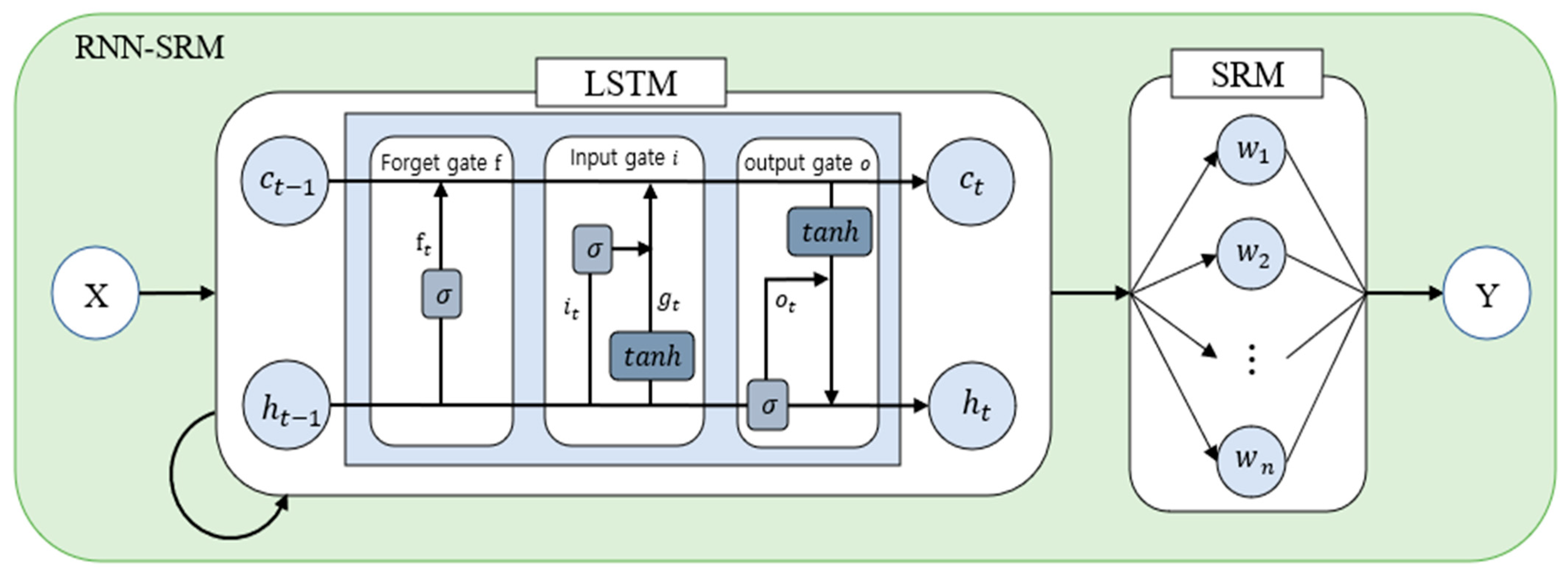
Here, $s_{min}$and $s_{max}$ denote the common minimum and maximum values calculated from both the input and target values in each training fold. The same scaling parameters were applied to the corresponding validation data to prevent information leakage. The observations were supplied chronologically using a batch size of 1 without random shuffling. The input tensor had the form $(1,1,1)$, corresponding to one sample, one time step, and one feature. A stateful LSTM was used to retain sequential information across consecutive observations. The values processed by the LSTM at each time point were transformed through a dense layer and subsequently supplied to a custom activation layer incorporating the SRM introduced in Section 2. The trainable quantities in this layer are the structural activation parameters $a$, $\alpha$, $\beta$, and $k$, which are jointly updated with the remaining neural-network weights through backpropagation. The output of the SRM-informed layer is then passed through a linear dense layer to produce the final prediction [21]. The structure of the proposed RNN-SRM is illustrated in Figure 2 [21].

Figure 2. The structure of RNN SRM.

Figure 2 presents a simplified conceptual representation. The actual computational implementation additionally includes a dense transformation layer before the SRM-informed activation and a linear dense layer after the activation.

This structure produces the final prediction through the following computational process. First, the normalized input $x_t^{\ast }$ is supplied to the LSTM structure introduced in Section 3.3.1, producing a hidden representation $h_t$ at each time point. The LSTM output is subsequently transformed by a dense layer as $z_t=W_z{z}_t+b_z$, where $W_z$ and $b_z$ denote the time-shared dense-layer weight matrix and bias vector, and $z_t$ represents a learned latent feature vector. Therefore, $z_t$ is not interpreted as physical time but as a latent representation of the sequential failure information. The mathematical structure of Equation (8) is incorporated into an activation layer parameterized by the structural activation parameters $a$, $\alpha$, $\beta$, and $k$.

Because each component $z_{t,j}$, where $j$ indexes the units of the dense layer, may take a negative value, directly calculating ${\left(\beta z_{t,j}\right)}^{\alpha }$ may produce an undefined real value when $\alpha$ is non-integer. To address this issue, the following sign-preserving power transformation is introduced [39]:

$$q\left(z_{t,j}\right)=sign\left(z_{t,j}\right){\left[{\left(\beta z_{t,j}\right)}^2\right]}^{\alpha /2}$$

The squared term ensures a non-negative base, while the sign function preserves the direction of the original latent feature. Let $g\left(z_{t,j}\right)$ denote the output obtained by applying the SRM-informed activation to the $j$th latent feature at time $t$. The mathematical structure of Equation (8) is applied to the transformed latent feature $q\left(z_{t,j}\right)$.

$$g\left(z_{t,j}\right)={\displaystyle \frac{a}{1+\frac{a-k}{k}·exp\left(-a·q\left(z_{t,j}\right)\right)}}, j=\mathrm{1,2},\cdots J$$

(14)

For $z_{t,j}>0$, the sign-preserving transformation reduces to the original power term ${\left(\beta z_{t,j}\right)}^{\alpha }$, while $q\left(0\right)=0$ ensures that $g\left(0\right)=k$. Negative values of $z_{t,j}$ do not represent negative physical time but indicate the direction of the learned latent feature. In the computational implementation, the exponent $-a·q\left(z_{t,j}\right)$ was restricted to the interval $\left[-40, 40\right]$ before applying the exponential function to prevent numerical overflow and underflow. In addition, a small positive constant was added to the denominator to avoid numerical instability when the denominator approached zero.

• The SRM-informed activation in Equation (14) is applied separately to each component of the latent feature vector. The resulting activation outputs are subsequently combined through a final linear dense layer.

  $${\widehat{y}}_t^{\ast }=b_o+{\displaystyle \sum _{j=1}^J}{v}_{j}g\left(z_{t,j}\right)$$

Here, $v_j$ denotes the weight connecting the $j$th SRM-informed activation output to the final output node, $b_o$ is the output-layer bias, and ${\widehat{y}}_t^{\ast }$ is the predicted normalized first difference at time $t$. Thus, $a$, $\alpha$, $\beta$, and $k$ determine the form of the SRM-informed activation, whereas $v_j$ and $b_o$ aggregate the activation outputs to produce the final DL-BPE prediction.

The structural activation parameters $a$, $\alpha$, $\beta$, and $k$ determine the mathematical form of the SRM-informed activation and are jointly updated with the remaining neural-network weights. Because the activation operates on latent features rather than physical time, these structural activation parameters are interpreted within the DL-BPE architecture rather than as numerically identical to the classical NHPP parameters estimated directly by LSE or MLE. The predicted normalized first differences were transformed back to their original scale and added to the preceding observed cumulative failure counts. The resulting cumulative predictions were constrained to be nondecreasing over time. The DL-BPE was trained by minimizing the mean squared error between the observed and predicted normalized first differences.

$$L\left(\Theta \right)={\displaystyle \frac{1}{N}}{\displaystyle \sum _{i=1}^N}{\left({y_i^{\ast }-\widehat{y}}_i^{\ast }\right)}^2$$

Here, $i$ indexes the supervised samples within each training fold, $N$ is the total number of samples in that fold, and $y_i^{\ast }$ and ${\widehat{y}}_i^{\ast }$ denote the observed and predicted normalized first differences for the $i$th sample, respectively. The parameter set $\Theta$ includes all trainable weights in the DL-BPE. The MSE of the reconstructed cumulative validation predictions was used for hyperparameter selection. The DL-BPE was trained using Adam for up to 150 epochs with a batch size of 1, and the observations were supplied sequentially without random shuffling. The hyperparameter search space included LSTM unit values of 4, 8, 16, and 24, learning rates of 0.001, 0.002, 0.005 and 0.01. Grid search was performed over all candidate combinations, and the weights yielding the lowest cumulative validation MSE were retained for each cross-validation fold.

Within each cross-validation fold, $a$ and $k$ were initialized using the maximum and initial number of failures, respectively, from that fold’s training window. The initial value of $\alpha$ was sampled from the convexity-preserving ranges $\left[0.1,1\right)$and $\left(2,10\right]$ whereas $\beta$ was sampled from $\left[0.1, 2\right]$. During training, the positivity and ordering constraints were enforced through reparameterization. Specifically, $k$ was defined as a strictly positive quantity, and $a$ was defined relative to $k$ so that $a>k$ was maintained throughout training. The parameters $\alpha$ and $\beta$ were also constrained to remain within their prespecified positive ranges. This construction guaranteed $0<k<a$ and prevented invalid parameter values during optimization. Hyperparameter tuning was conducted using a fixed seed of 5001. After the hyperparameters were selected, the DL-BPE model was independently trained 40 times using 40 distinct prespecified random seeds ranging from 1001 to 1040. The use of different random seeds generated different stochastic initializations while keeping the model architecture and hyperparameter settings unchanged, allowing the run-to-run variability of DL-BPE to be examined. Because the training results may be sensitive to stochastic initialization, the training run with the lowest Train MSE was selected for reporting the parameter estimates and predictive results, while the distribution of the results across all 40 training runs was also examined to assess variability. The DL-BPE analysis was implemented in R using keras and TensorFlow (R 4.5.0; keras 2.15.0; tensorflow 2.16.0).

4. Numerical Example

This section empirically evaluates the proposed convex-dependent NHPP SRM using three software failure datasets. First, the fitting performance of the proposed model is compared with that of existing NHPP SRMs to examine its ability to represent different software failure patterns. Next, the parameters of the proposed model are estimated using LSE, MLE, and the proposed DL-BPE method, and the resulting fitting and predictive performance is compared across the three estimation approaches. Through these analyses, the applicability of both the proposed SRM and the DL-BPE estimation framework is examined.

4.1. Data Information

The first dataset measured errors from the Shuttle Ground Processing System (SGPS), a software system used by NASA to monitor, analyze, and control spacecraft flights from the ground. It captures instances in which the program does not operate as planned during execution, including incorrect calculation results, command processing errors, abnormal terminations, and unexpected behavior. Measurements were taken over approximately 38 weeks, accumulating data on errors observed over 2800 h of cumulative test time. Failure data were categorized into three types: critical errors (errors rendering mission execution impossible), major errors (errors severely impacting core functionality), and minor errors (errors causing significant system operation issues). This study combines these categories for the analysis [40].

The second dataset utilizes failure data from Hive, which is based on Apache open-source software. Hive is a distributed fault-tolerant data warehouse system built on Apache Hadoop, which enables large-scale analyses. It allows reading, writing, and management of petabyte-scale data. This dataset is defined across five releases and contains information on defects and failures that occurred between 2008 and 2014 [41].

The third dataset includes failures and defects occurring during the development of real-time multi-computer system software for the naval tactical data system (NTDS). The NTDS comprises 38 modules, each of which records and measures the errors generated during the production, testing, and user phases. A total of 26 errors were found during the production phase, five during the testing phase, and three during the final user phase. These three datasets were used to validate the effectiveness of the proposed model [6].

4.2. Evaluation Criteria

To evaluate the performance of the proposed SRM, we compared it to traditional models using multiple criteria. The eight criteria were compared as shown in Table 2. In Table 2, $\widehat{m}\left(t_i\right)$ denotes the estimated value at time $t_i$, $y_i$ denotes the corresponding observed value, $i$ is the observation index, $n$ is the number of observations, and $m$ is the number of parameters.

Table 2. Criteria.

No.	Criteria	Formula
1	MSE [42]	${\displaystyle \frac{{\sum }_{i=1}^n{\left(\widehat{m}\left(t_i\right)-y_i\right)}^2}{n-m}}$
2	PRR [43]	${\displaystyle \sum _{i=1}^n}{\left({\displaystyle \frac{\widehat{m}\left(t_i\right)-y_i}{\widehat{m}\left(t_i\right)}}\right)}^2$
3	PP [43]	${\displaystyle \sum _{i=1}^n}{\left({\displaystyle \frac{\widehat{m}\left(t_i\right)-y_i}{y_i}}\right)}^2$
4	MAE [44]	${\displaystyle \frac{{\sum }_{i=1}^n\left|\widehat{m}\left(t_i\right)-y_i\right|}{n-m}}$
5	RMSPE [44]	$\sqrt{{\displaystyle \frac{{\sum }_{i=1}^n{\left(y_i-\widehat{m}\left(t_i\right)-{\sum }_{i=1}^n\left[\frac{\widehat{m}\left(t_i\right)-y_i}{n}\right]\right)}^2}{n-1}}+{{\displaystyle \sum _{i=1}^n}\left[{\displaystyle \frac{\widehat{m}\left(t_i\right)-y_i}{n}}\right]}^2}.$
6	MEOP [44]	${\displaystyle \frac{{\sum }_{i=1}^n\left|\widehat{m}\left(t_i\right)-y_i\right|}{n-m+1}}$
7	PC [45]	${\displaystyle \frac{n-m}{2}}\ast \mathit{log}\left({\displaystyle \frac{{\sum }_{i=1}^n{\left(\widehat{m}\left(t_i\right)-y_i\right)}^2}{n}}\right)+\mathrm{m}\left({\displaystyle \frac{n-1}{n-m}}\right)$
8	${Adj\_R}^2$ [46]	$1-{\displaystyle \frac{\left(1-R^2\right)\left(n-1\right)}{n-m-1}}$

The mean squared error (MSE) is a measure that considers the sum of the squares of the differences between the estimated and actual values, weighted by the number of observations and parameters. The predictive ratio risk (PRR) and predictive power (PP) were defined as the difference between the predicted and actual values divided by the predicted and actual values, respectively, for model estimation. The adjusted ${\mathrm{R}}^2$ (Adj_R²) is the adjusted coefficient of determination for a regression equation derived from the coefficient of determination and accounts for the number of parameters; it assesses the explanatory power. The mean absolute error (MAE) is a measure that accounts for the number of observations and parameters and is calculated as the sum of the absolute differences between the estimated and actual values. The root mean square prediction error (RMSPE) estimates the closeness of predictions made by each model. The mean error of prediction (MEOP) was defined as the sum of the absolute deviations between the actual and estimated values. The Pham’s criterion (PC) is a measure that considers the number of parameters by increasing the penalty each time a parameter is added to a model when the sample size is small.

Based on these metrics, we compared existing NHPP SRMs with the proposed model. A higher Adj_R² value indicates a better fit, whereas the other seven metrics indicate a better fit when closer to zero. Using R 4.5.0 and MATLAB R2024b, we estimated parameters via LSE based on the difference between the model-estimated values and the actual number of failures, calculated criteria, and compared their performances.

4.3. Results of Analysis

4.3.1. Results of Dataset 1

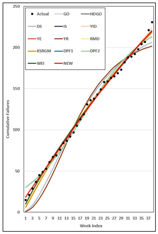
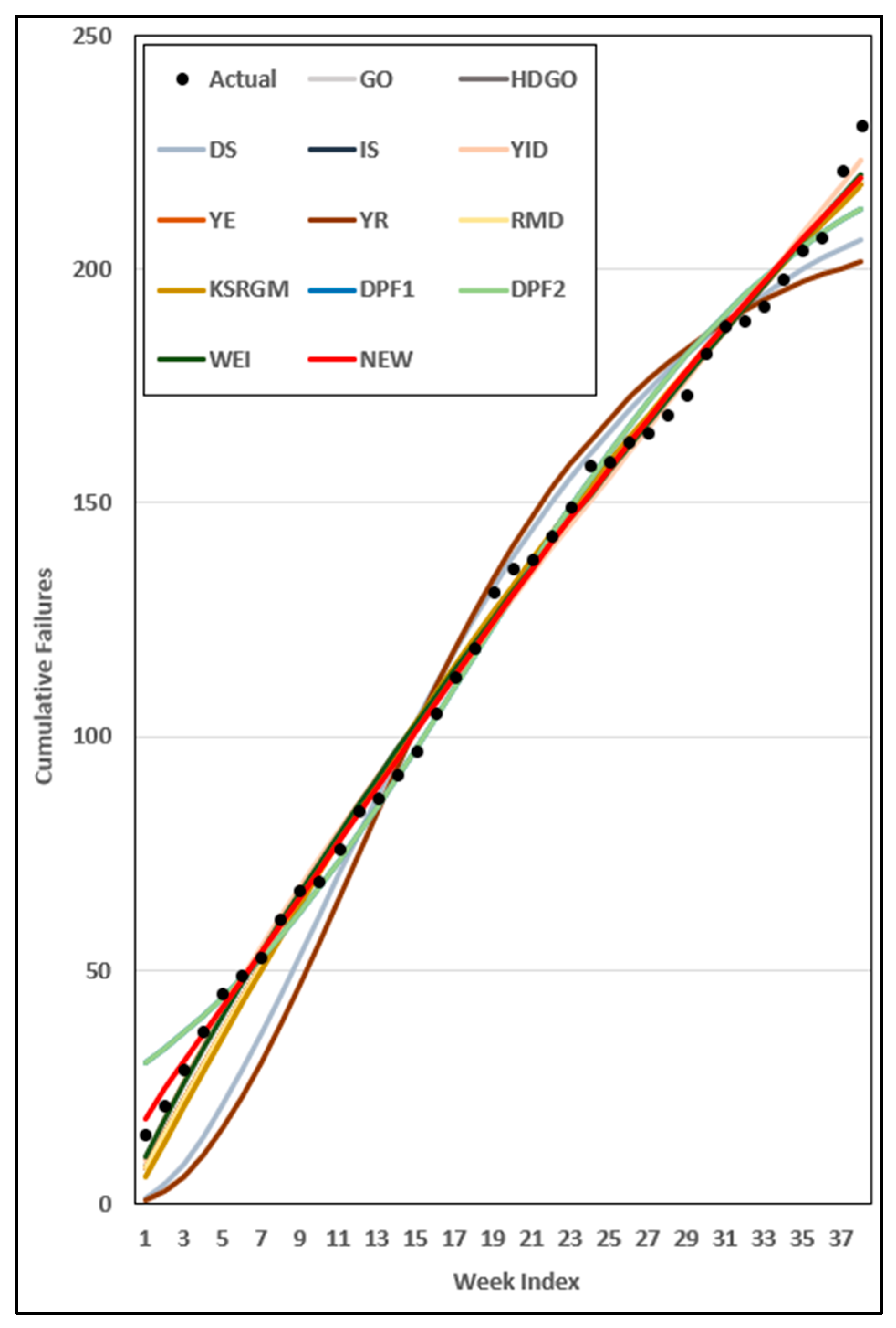
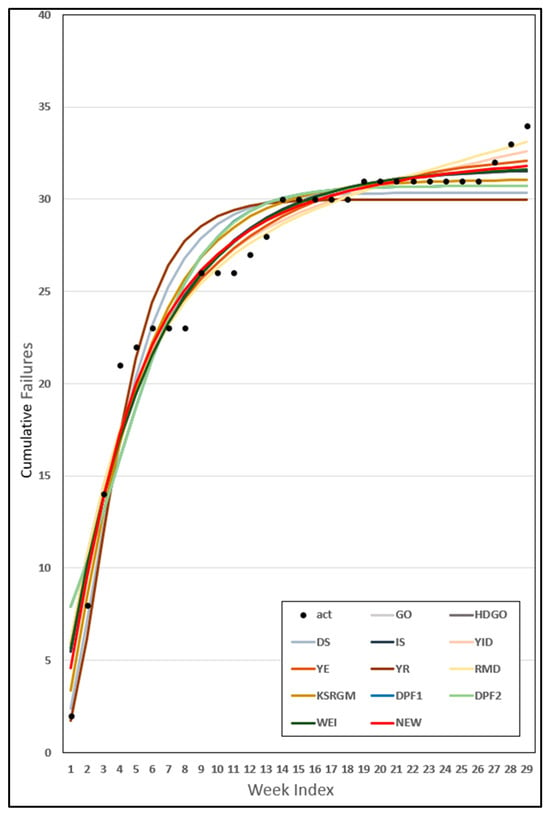
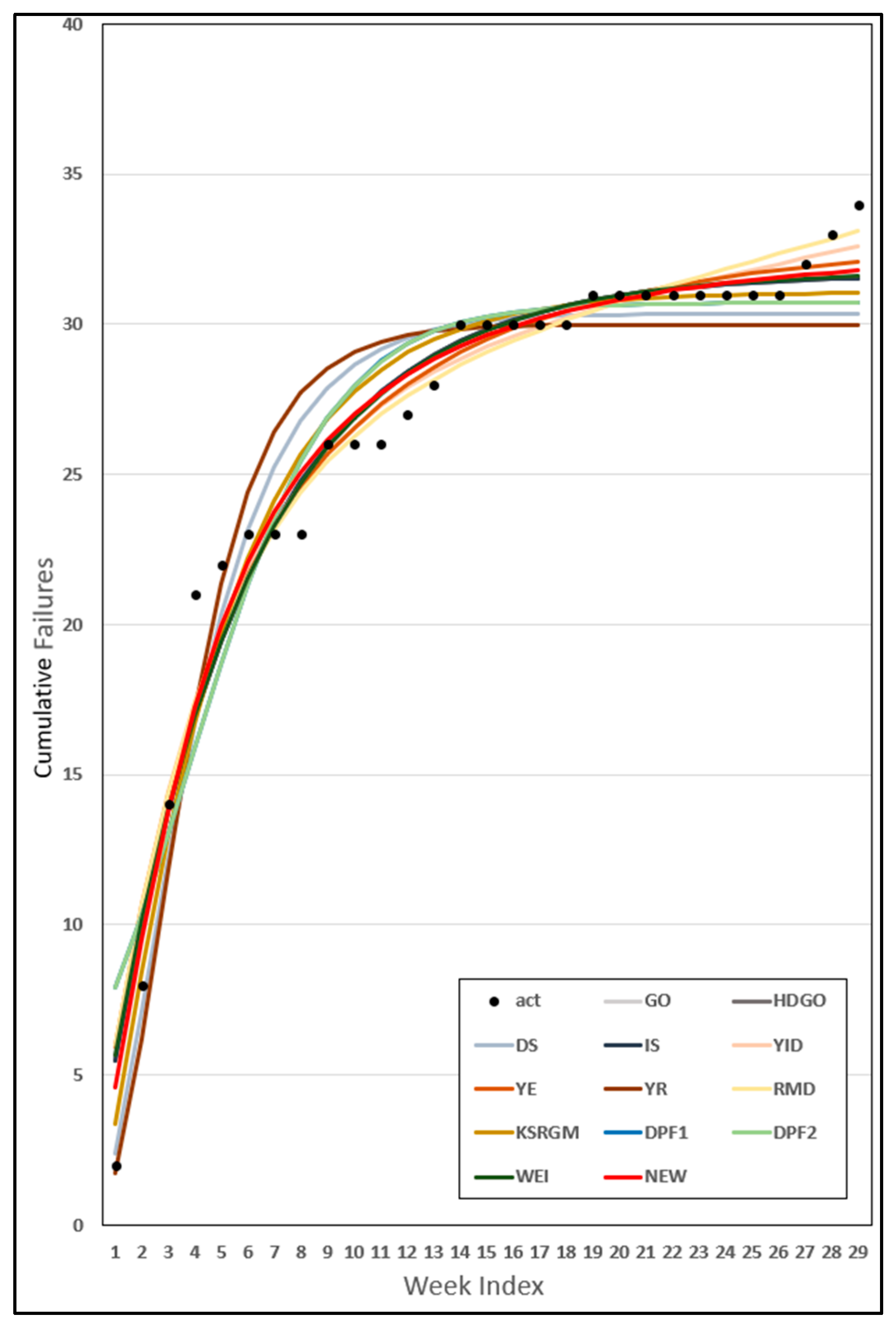
Table 3 shows the estimated parameters for each model compared with dataset 1. The estimated parameters for the proposed model are total number of failures $\widehat{a}$ = 365.9240, initial number of failures $\widehat{k}$ = 7.2220, shape parameter $\widehat{\alpha }$ = 0.4115, and scale parameter $\widehat{\beta }$ = 0.00000054. Table 4 presents the criteria calculated using the parameter estimates obtained from Table 3 for each model. The analysis showed that it yielded the best results across all eight criteria. The model assuming another convex form, that is, the Weibull distribution, also showed the second-best results. The previously proposed models, viz., DPF1 and DPF2, which assume dependent failure occurrence, were found to be poorly estimated for this dataset. Figure 3 shows the results at each time point based on the estimated parameter values for each model in Table 3. The black dots represent the actual data points and the red solid lines indicate the estimated values from the proposed SRM. Most models exhibited trends similar to the actual values, with the proposed model exhibiting results that were very close to the actual values from the starting point to the final time point.

Table 3. Parameter estimation from dataset 1.

Model	$\widehat{\mathit{a}}$	$\widehat{\mathit{b}}$	$\widehat{\mathit{\alpha }}$	$\widehat{\mathit{\beta }}$	$\widehat{\mathit{k}}$, $\widehat{\mathit{\gamma }}$	$\widehat{\mathit{c}}$	$\widehat{\mathit{p}}$, $\widehat{\mathit{h}}$
GO	475.5038	0.0162
HDGO	475.5039	0.0162				2.5855
DS	230.3591	0.1010
IS	475.3702	0.0162		0.0005
YID	56.0484	0.1760	0.0923
YE	833.3409		0.1424	0.0081	8.0558
YR	249.6582		0.3024	0.0029	6.2103
RMD	112.2567	0.0187	4.6744	0.0079
KSRGM	414.3523	19.5799	0.0370				0.0010
DPF1	236.2619	0.0001				0.1431	31.0786
DPF2	236.1932	0.0005				0.0025	31.0311
WEI	1220.8527		0.8780	0.0042
NEW	365.9240		0.4115	0.00000054	7.2220

Table 4. Comparison of criteria from dataset 1.

Model	MSE	PRR	PP	MAE	RMSPE	MEOP	PC	Adj_R2
GO	21.2346	1.3014	0.4733	3.8514	4.5436	3.7473	56.0837	0.9943
HDGO	21.8409	1.3026	0.4736	3.9587	4.5435	3.8487	55.6985	0.9941
DS	133.3463	187.1664	3.1075	9.298	11.3759	9.0467	89.1554	0.964
IS	21.8465	1.3067	0.4747	3.9512	4.5438	3.8415	55.703	0.9941
YID	16.6987	0.418	0.2054	3.6397	3.9743	3.5386	51.0005	0.9955
YE	22.1273	1.2731	0.4655	4.0252	4.5067	3.9102	55.1079	0.994
YR	221.7924	518.4964	4.0693	12.6706	14.2539	12.3086	94.2917	0.9401
RMD	22.3584	1.2892	0.47	4.0678	4.5309	3.9516	55.2846	0.994
KSRGM	27.8595	3.1491	0.7355	4.4155	5.057	4.2894	59.0241	0.9925
DPF1	41.3669	0.4865	1.503	4.9415	6.1652	4.8004	65.7443	0.9888
DPF2	41.3145	0.485	1.4954	4.9326	6.1613	4.7917	65.7227	0.9888
WEI	16.0327	0.3573	0.1952	3.4828	3.8941	3.386	50.2883	0.9957
NEW	15.5257	0.0854	0.1105	3.2702	3.7771	3.1767	49.0846	0.9958

Figure 3. Prediction for dataset 1.

4.3.2. Results of Dataset 2

Table 5 presents the estimated parameters for each model compared with dataset 2. The estimated parameters for the proposed model are: $\widehat{a}$ = 4683.9770, $\widehat{k}$ = 221.4734, $\widehat{\alpha }$ = 0.0000032, $\widehat{\beta }$ = 0.8474. Table 6 presents the results for the criteria calculated using the estimated values of each model, based on the parameter estimates obtained from Table 5. The proposed model showed the best results for MAE, MEOP, and PC with 66.8365, 65.5754, and 230.8538, respectively, and the second-best results for MSE, RMSPE, and Adj_R² with 6570.717, 78.8134, and 0.9859, respectively. The IS model showed the best results in terms of MSE, RMSPE, and Adj_R² with values of 6214.1, 77.345, and 0.9867, respectively. It exhibited the second-best results for MAE, MEOP, and PC at 66.9681, 65.728, and 233.1204, respectively. Thus, the proposed and IS models emerged as the best-performing models on this dataset.

Table 5. Parameter estimation from dataset 2.

Model	$\widehat{\mathit{a}}$	$\widehat{\mathit{b}}$	$\widehat{\mathit{\alpha }}$	$\widehat{\mathit{\beta }}$	$\widehat{\mathit{k}}$, $\widehat{\mathit{\gamma }}$	$\widehat{\mathit{c}}$	$\widehat{\mathit{p}}$, $\widehat{\mathit{h}}$
GO	183,078.71	0.0002
HDGO	709.4483	0.1542				0.4184
DS	3592.1670	0.0391
IS	87,134.617	0.0111		28.8987
YID	1918.7578	0.0164	0.0335
YE	384,498.63		2.4628	0.0002	0.2179
YR	3746.4441		1.2515	0.0007	1.1662
RMD	36,413.628	0.0037	1.2370	0.0042
KSRGM	15,598.845	3.6291	3.9709				0.0007
DPF1	4697.3960	0.00000022				0.0200	293.8370
DPF2	4695.9395	0.0000139				0.2617	293.8313
WEI	33,575.982		0.0019	1.1557
NEW	4683.9770		0.0000032	0.8474	221.4734

Table 6. Comparison of criteria from dataset 2.

Model	MSE	PRR	PP	MAE	RMSPE	MEOP	PC	Adj_R2
GO	11,551.67	0.3546	0.3157	77.778	106.4875	76.3638	253.6289	0.9753
HDGO	656,171	70.4816	15.314	605.2459	792.1579	594.0376	356.5998	0.3774
DS	22,255.74	412.638	6.5276	131.2098	147.6921	128.8241	271.3347	0.9524
IS	6214.1	1.694	0.9682	66.9681	77.345	65.728	233.1204	0.9867
YID	7333.871	1.8079	1.0101	71.8703	84.0389	70.5393	237.511	0.9843
YE	12,084.42	0.3518	0.3167	81.6226	106.8763	80.0825	246.6955	0.9741
YR	31,285.19	943.4873	8.1067	158.3062	171.7957	155.3193	271.4274	0.933
RMD	7185.538	1.5983	0.9238	71.7033	82.4028	70.3504	233.1794	0.9846
KSRGM	8337.017	13.9152	2.3823	79.5947	88.7069	78.093	237.0439	0.9821
DPF1	7740.321	2.1647	34.1433	74.7453	85.5376	73.335	235.1131	0.9834
DPF2	7725.274	2.1684	34.1287	74.1435	85.459	72.7445	235.0625	0.9835
WEI	9016.589	3.8183	1.5172	80.2086	93.1884	78.7233	242.9849	0.9807
NEW	6570.717	1.8131	22.2746	66.8365	78.8134	65.5754	230.8538	0.9859

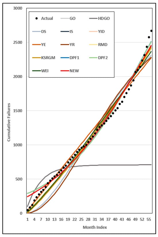
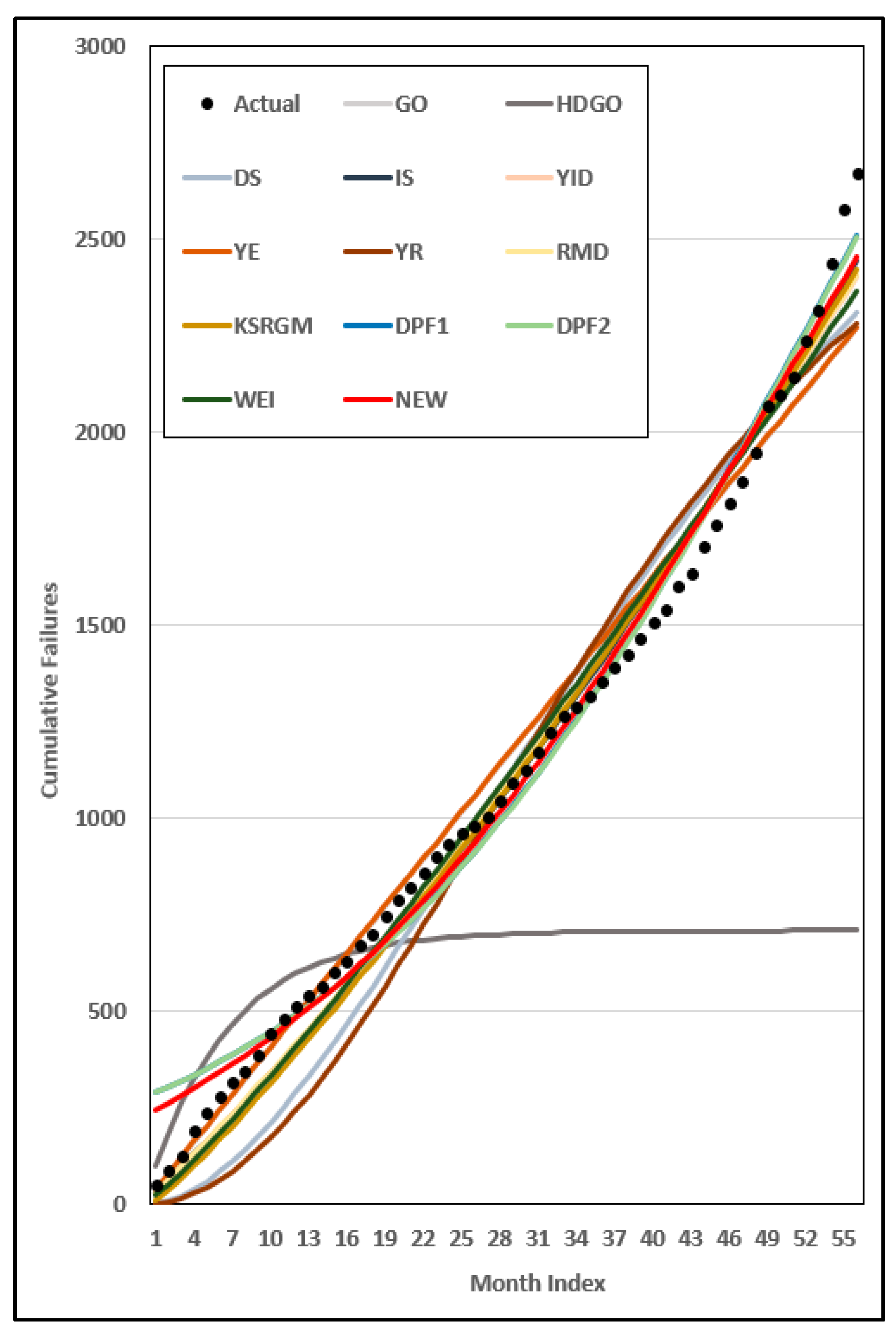
Figure 4 shows the results for each time point, which are similar to those in Section 4.3.1. The black dots represent the actual data and the solid red line represents the estimated values from the proposed SRM. Because the proposed model assumes that failures occur early, it exhibits high values at the initial points and fits well thereafter.

Figure 4. Prediction for dataset 2.

4.3.3. Results of Dataset 3

Table 7 presents the estimated parameters for each model compared using dataset 3. The estimated parameters for the proposed model are: $\widehat{a}$ = 32.8052, $\widehat{k}$ = 0.000091, $\widehat{\alpha }$ = 0.000075, $\widehat{\beta }$ = 0.1151. Table 8 presents the results for the criteria calculated using the estimated values from each model, based on the parameter estimates obtained from Table 7. The proposed model achieved the best results for MSE, RMSPE, MEOP, PC, and Adj_R², with values of 1.9352, 1.3144, 1.0380, 10.8775, and 0.9634, respectively. It also achieved the second-best result for MAE at 1.0796 and ranked fourth for PRR and PP, indicating competitive overall performance. The DS model exhibited the best results for PRR and PP, with values of 0.2299 and 0.2176, respectively. Figure 5 shows the results for each time point, which are similar to those in Section 4.3.1. Despite the periods of stagnation inherent in the data, the models showed similar trends and exhibited a distribution with minimal deviation from the actual values.

Table 7. Parameter estimation from dataset 3.

Model	$\widehat{\mathit{a}}$	$\widehat{\mathit{b}}$	$\widehat{\mathit{\alpha }}$	$\widehat{\mathit{\beta }}$	$\widehat{\mathit{k}}$, $\widehat{\mathit{\gamma }}$	$\widehat{\mathit{c}}$	$\widehat{\mathit{p}}$, $\widehat{\mathit{h}}$
GO	31.6557	0.1906
HDGO	31.6556	0.1906				0.0002
DS	30.3528	0.4601
IS	31.6531	0.1908		0.0020
YID	28.0366	0.2370	0.0066
YE	33.9404		1.3972	0.0539	2.6227
YR	31.4494		1.5291	0.0372	2.0018
RMD	75.8633	0.2498	1.3541	0.0034
KSRGM	11.0124	5.5814	0.6455				0.1306
DPF1	30.7156	0.0010				0.0827	7.3263
DPF2	30.7196	0.0124				0.0172	7.3124
WEI	31.7543		0.1895	0.9810
NEW	32.8052		0.000075	0.1151	0.000091

Table 8. Comparison of criteria from dataset 3.

Model	MSE	PRR	PP	MAE	RMSPE	MEOP	PC	Adj_R2
GO	2.3072	0.5512	3.1953	1.0892	1.4915	1.0503	12.3957	0.9565
HDGO	2.3959	0.5512	3.1954	1.1311	1.4915	1.0892	13.1699	0.9547
DS	3.7909	0.2299	0.2176	1.5335	1.9119	1.4787	19.0996	0.9285
IS	2.3969	0.5510	3.1904	1.1313	1.4918	1.0894	13.1752	0.9547
YID	2.0935	0.5754	4.0429	1.0784	1.3941	1.0384	11.416	0.9604
YE	2.3088	0.5825	4.0485	1.1378	1.4357	1.0941	13.084	0.9563
YR	5.3829	0.3322	0.2862	1.9739	2.1922	1.8979	23.6652	0.8981
RMD	2.2449	0.5823	4.1073	1.1358	1.4157	1.0921	12.7332	0.9575
KSRGM	2.6484	0.3017	0.5851	1.2403	1.5377	1.1926	14.799	0.9499
DPF1	5.1291	0.8124	8.9603	1.7358	2.1399	1.669	23.0614	0.9029
DPF2	5.1126	0.8113	8.9475	1.7316	2.1365	1.665	23.0212	0.9032
WEI	2.3915	0.5644	3.4651	1.127	1.4901	1.0852	13.1463	0.9548
NEW	1.9352	0.4284	1.7697	1.0796	1.3144	1.038	10.8775	0.9634

Figure 5. Prediction for dataset 3.

4.4. Parameter Estimation Comparison Results

Section 4.3 showed that the proposed convex-dependent SRM achieved competitive fitting performance across the datasets. This Section compares the proposed DL-BPE framework with LSE and MLE to examine its predictive performance under the proposed convex-dependent NHPP SRM. To estimate the parameters using DL-BPE, the hyperparameters were specified via cross-validation. Given the sequential nature of the failure data, expanding-window cross-validation was employed to tune these hyperparameters [47,48]. For model development and performance evaluation, the entire dataset was first chronologically divided into a training set comprising the first 80% of the observations and a test set comprising the remaining 20%. Hyperparameter tuning was conducted exclusively within the training set using an expanding-window cross-validation scheme. Specifically, the initial training window consisted of the first 60% of the entire dataset, and the training window was subsequently expanded by one observation at a time until reaching the 80% boundary. At each step, the observation immediately following was used as the validation sample. This procedure resulted in 7, 11, and 6 validation folds for datasets 1, 2, and 3, respectively, with a one-step-ahead forecast horizon. The hyperparameters were tuned using a grid search to identify the optimal configuration under the predefined conditions [49]. The number of hidden nodes was set to 4, 8, 16, and 24, while the learning rate was set to 0.001, 0.002, 0.005, and 0.01. The total number of epochs was set to 150. After the optimal hyperparameter combination was selected based solely on the cross-validation results within the training set, the model was retrained using the entire 80% training set. The remaining 20% test set was used exclusively for final out-of-sample performance evaluation and was not involved in hyperparameter tuning or model training. Among the 40 independent training runs, the run with the lowest Train MSE was selected based solely on the training set. The model obtained from the selected training run was subsequently evaluated on the test set, and the test-set performance was not used for run selection. Table 9 presents the results of the expanding-window cross-validation used for hyperparameter selection. For datasets 1, 2, and 3, the selected numbers of hidden-layer nodes were 24, 8, and 16, respectively, while the corresponding learning rates were 0.005, 0.005, and 0.010. The mean cross-validation MSE values were 0.29977, 12.59182, and 0.00610, with standard deviations of 0.47579, 16.78679, and 0.00985, respectively. These results represent the hyperparameter combinations selected on the basis of their validation performance under the expanding-window cross-validation procedure. The variability in validation errors differed across datasets, with dataset 2 showing greater variation across validation folds than datasets 1 and 3.

Table 9. Hyperparameter tuning via cross-validation from the datasets.

Dataset	Hidden-Layer Nodes	Learning Rate	CV_MSE_Mean	CV_MSE_SD
Dataset 1	24	0.005	0.29977	0.47579
Dataset 2	8	0.005	12.59182	16.78679
Dataset 3	16	0.010	0.00610	0.00985

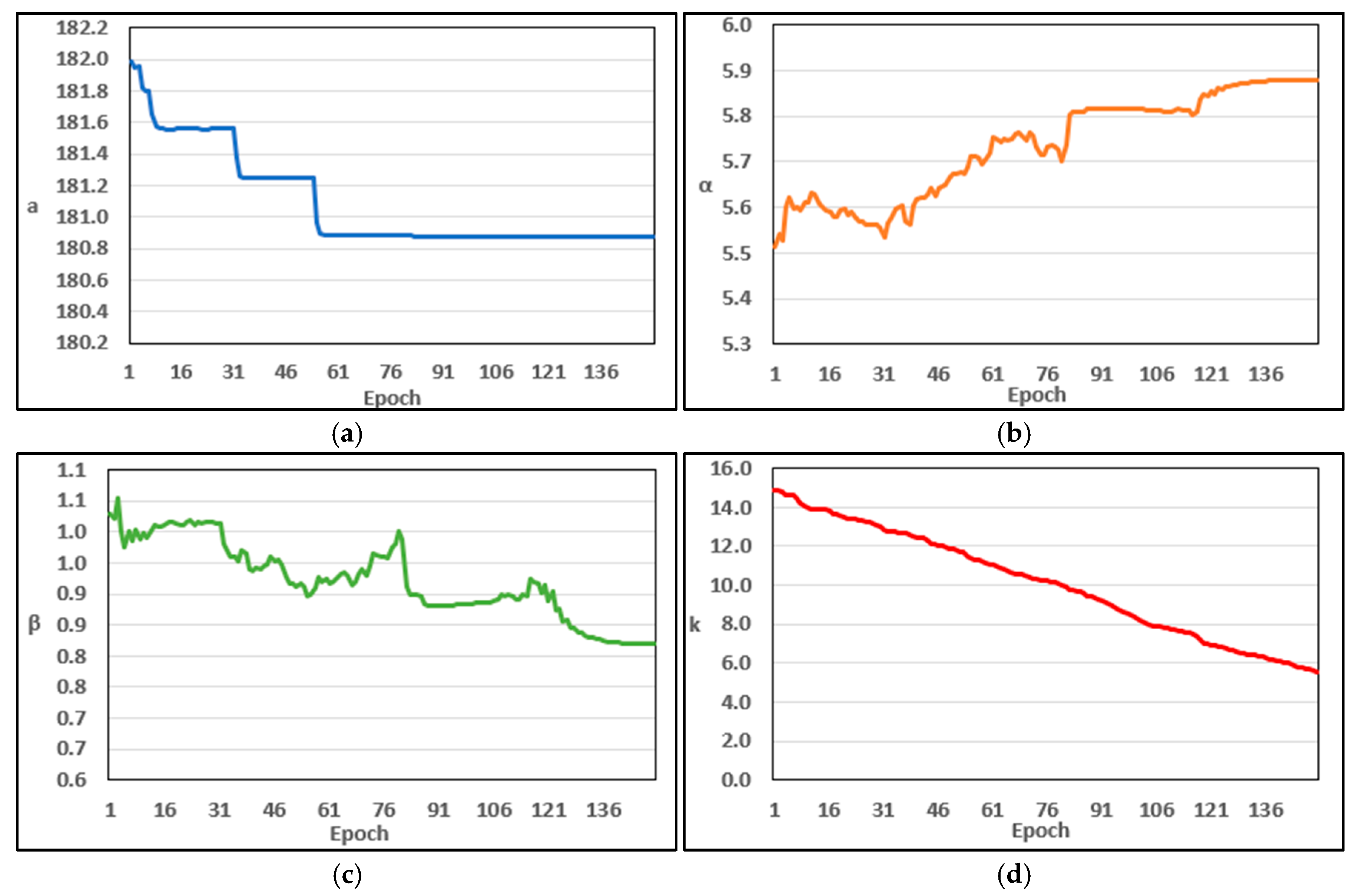
Table 10 presents the parameter estimation results for the proposed model based on dataset 1 using LSE, MLE, and the proposed DL-BPE method. The parameter estimates obtained using DL-BPE were $\widehat{a}$ = 180.8720, $\widehat{\alpha }$ = 5.8789, $\widehat{\beta }$ = 0.8191, and $\widehat{k}$ = 5.5766. Figure 6 shows how each parameter changed over 150 epochs during DL-BPE training. The blue line represents $a$, the orange line represents $\alpha$, the green line represents $\beta$, and the red line represents $k$. The estimates of $a$ and $k$ generally decreased during training, while $\alpha$ showed an overall increasing trend and $\beta$ gradually decreased with moderate fluctuations. By the final epochs, all four parameters approached relatively stable values of approximately 180.8720, 5.8789, 0.8191, and 5.5766, respectively. In particular, the final estimate of $\widehat{\alpha }$ = 5.8789 indicates that the fault-detection process for dataset 1 was fitted to an increasing and convex structure.

Table 10. Parameter estimation results of the proposed model for dataset 1.

Method	$\widehat{\mathit{a}}$	$\widehat{\mathit{\alpha }}$	$\widehat{\mathit{\beta }}$	$\widehat{\mathit{k}}$
LSE	326.6145	0.4213	0.000001	6.9514
MLE	357.2662	0.4765	0.0000018	14.9888
DL-BPE	180.8720	5.8789	0.8191	5.5766

Figure 6. Changes in parameter values during DL-BPE training for dataset 1; (a) $a$; (b) $\alpha$; (c) $\beta$; (d) $k.$

Table 11 summarizes the results of the evaluation criteria calculated using the parameter estimates obtained from the 80% training dataset reported in Table 10. The evaluation criteria were used to assess the goodness-of-fit of each estimation method within the training dataset. In addition, prediction SSE (preSSE) was calculated for the remaining 20% test dataset using the parameter estimates obtained from the training dataset to evaluate predictive performance on the test dataset. The preSSE is defined as the sum of squared differences between the observed and predicted values in the test dataset, as follows:

$$preSSE={\displaystyle \sum _{i=k+1}^n}{\left(\widehat{m}\left(t_i\right)-y_i\right)}^2$$

where $k$ denotes the last time point of the training dataset, $n$ denotes the final time point of the entire dataset, $y_i$ denotes the observed value at time $t_i$, and $\widehat{m}\left(t_i\right)$ denotes the predicted value obtained from the estimated model. Thus, preSSE represents the sum of squared prediction errors over the test period from $k+1$ to $n$, with a smaller value indicating better predictive performance.

Table 11. Results of criteria between parameter estimation methods from dataset 1.

Method	MSE	PRR	PP	MAE	RMSPE	MEOP	PC	Adj_R2	preSSE
LSE	9.2256	0.0400	0.0444	2.6315	2.8700	2.5303	30.3995	0.9960	365.3327
MLE	9.5623	0.0298	0.0292	2.6462	2.9219	2.5444	30.8476	0.9958	331.0289
DL-BPE	7.5261	0.0272	0.0262	2.4438	2.5921	2.3498	27.8544	0.9967	123.2066

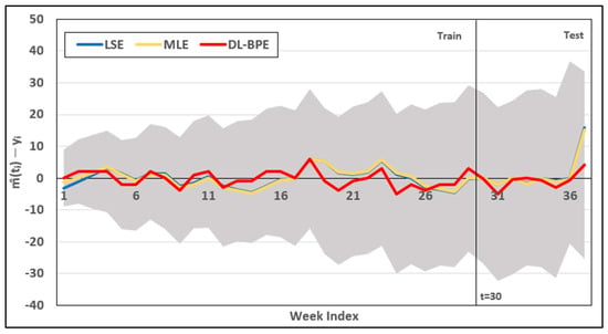
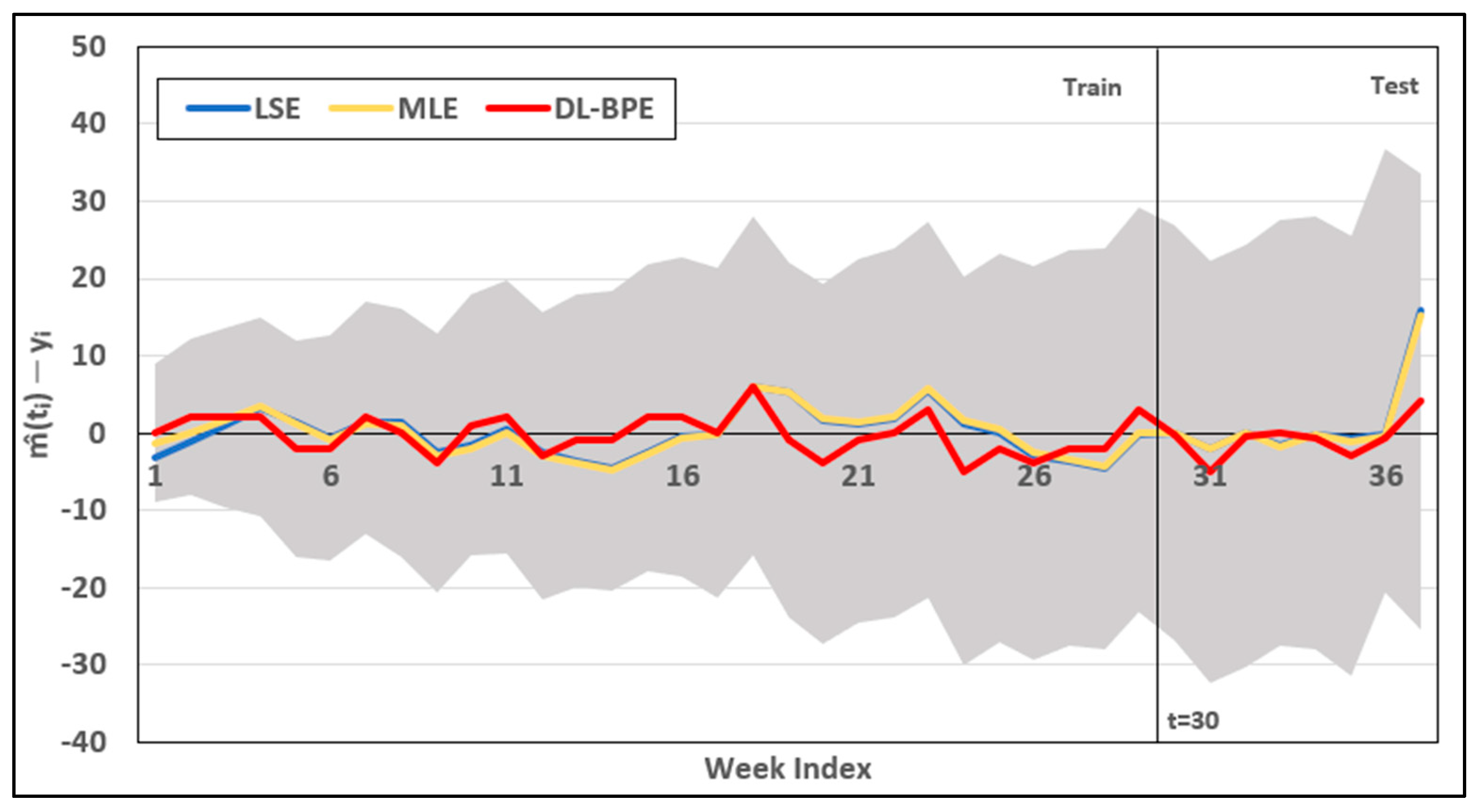
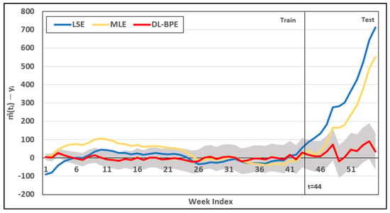
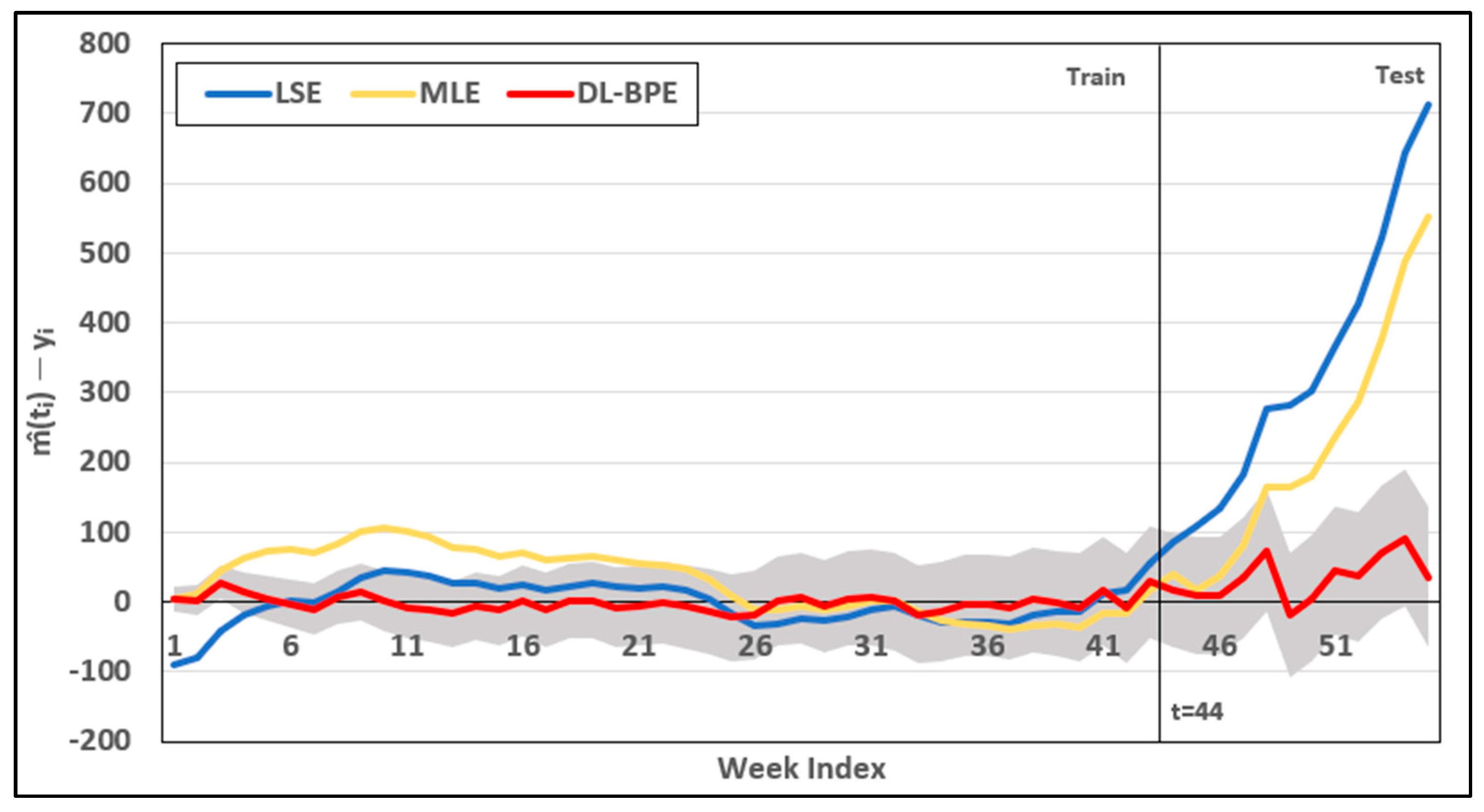
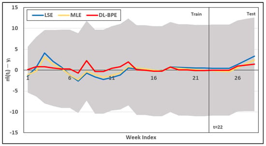
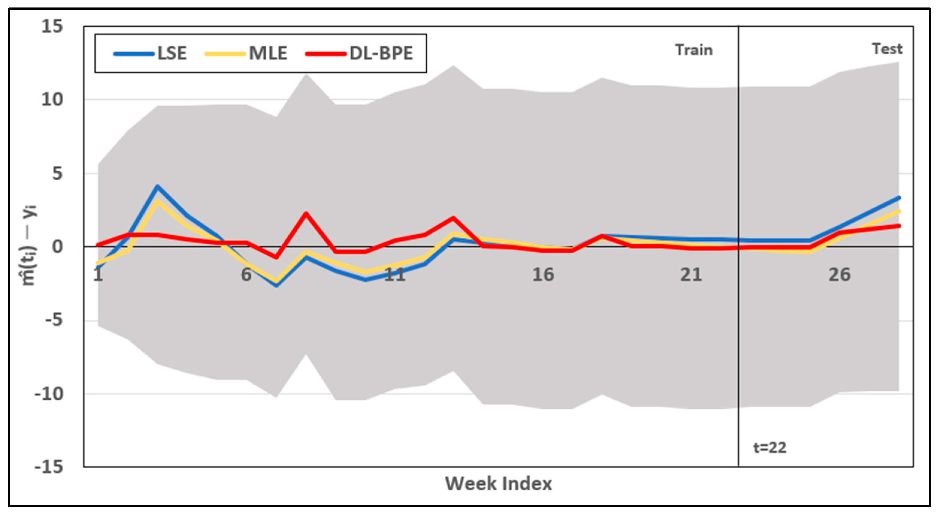
For dataset 1, DL-BPE produced the lowest preSSE of 123.2066, compared with 365.3327 for LSE and 331.0289 for MLE, indicating better predictive performance on the test dataset. Figure 7 shows the differences between the observed and estimated cumulative failure values at each time point for each estimation method. The blue, yellow, and red lines represent LSE, MLE, and DL-BPE, respectively. The gray shaded area represents the 95% Poisson-based interval derived from the mean value function estimated by DL-BPE and expressed on the same difference scale. In particular, the DL-BPE errors remaining within this shaded interval indicate that the corresponding observed cumulative failure values lie within the 95% Poisson-based interval around the DL-BPE estimates. Thus, the observed values were generally contained within the range expected under the estimated DL-BPE model across both the training and test periods. Across most time points, the differences for the three methods varied around zero, while DL-BPE generally showed smaller deviations from the observed values, particularly during the test period. Figure 7 distinguishes the training and test periods, with the first 80% of the data used for training and the remaining 20% used to evaluate predictive performance. In the test period, DL-BPE generally exhibited smaller prediction errors than LSE and MLE, particularly at the final time point.

Figure 7. Difference between observed and estimated cumulative failure values for dataset 1.

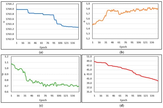
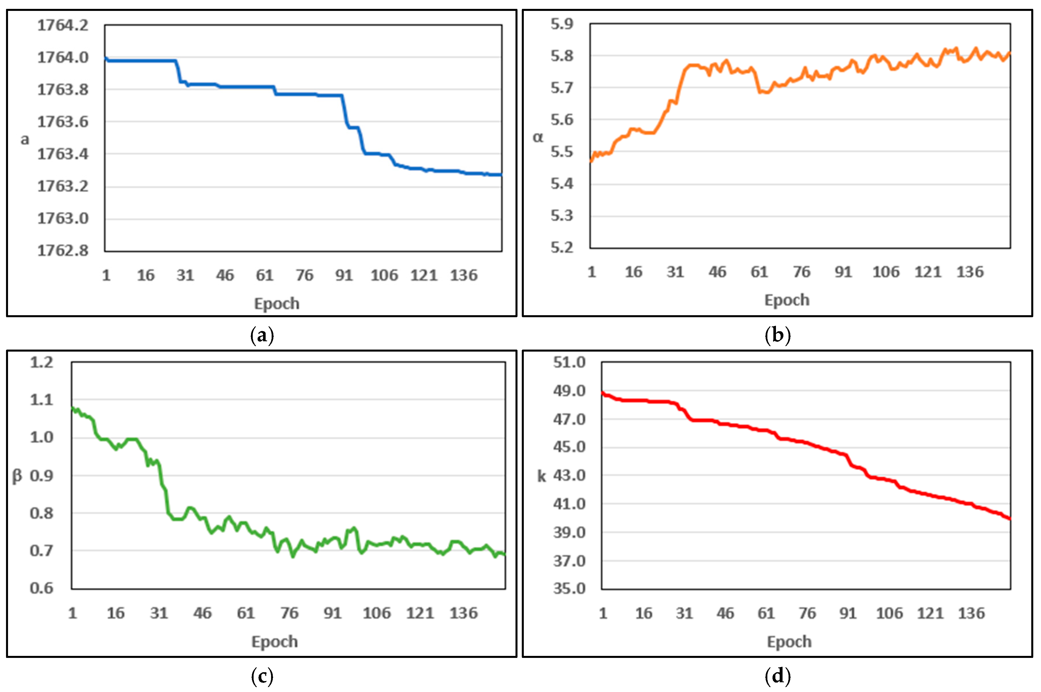
Table 12 presents the parameter estimation results for dataset 2 obtained using the LSE, MLE, and proposed DL-BPE. The estimated parameters derived from DL-BPE were $\widehat{a}$ = 1763.2719, $\widehat{\alpha }$ = 5.8082, $\widehat{\beta }$ = 0.6916, and $\widehat{k}$ = 39.9832. Figure 8 illustrates the changes in each parameter over 150 epochs during the DL-BPE, following the same color scheme described in the previous Figure 6. The parameter estimates show that $a$ and $k$ generally decreased, $\alpha$ increased, and $\beta$ gradually decreased with some fluctuations, with all parameters approaching relatively stable values toward the end of training. The final value of $\widehat{\alpha }$ = 5.8082 places the fitted model in the increasing and convex region of the fault-detection rate for dataset 2.

Table 12. Parameter estimation results of the proposed model for dataset 2.

Method	$\widehat{\mathit{a}}$	$\widehat{\mathit{\alpha }}$	$\widehat{\mathit{\beta }}$	$\widehat{\mathit{k}}$
LSE	2478.8998	0.6472	0.000001	110.2791
MLE	3264.2750	0.4528	0.00000001	48.9976
DL-BPE	1763.2719	5.8082	0.6916	39.9832

Figure 8. Changes in parameter values during DL-BPE training for dataset 2; (a) $a$; (b) $\alpha$; (c) $\beta$; (d) $k.$

Table 13 summarizes the evaluation criteria calculated based on the estimates reported in Table 12. In addition, preSSE was calculated using the test data to evaluate the predictive performance of each estimation method. For dataset 2, DL-BPE achieved substantially improved performance compared with LSE and MLE across the evaluation criteria and produced the lowest preSSE of 25,208. Figure 9 shows the differences between the observed and estimated cumulative failure values at each time point for each estimation method. The gray shaded area has the same interpretation as the 95% Poisson-based interval described for Figure 7. Figure 9 distinguishes the training and test periods, with the first 80% of the data used for training and the remaining 20% used for predictive performance evaluation. Overall, the LSE-based predictions exhibited the largest deviations from the observed values, particularly during the test period, whereas DL-BPE produced comparatively smaller prediction errors. During the test period, the errors of LSE and MLE exceeded the 95% interval at several later time points, whereas the DL-BPE errors remained largely within the interval.

Table 13. Results of criteria between parameter estimation methods from dataset 2.

Method	MSE	PRR	PP	MAE	RMSPE	MEOP	PC	Adj_R2	preSSE
LSE	1214.4039	0.5080	1.6093	29.5821	33.6106	28.8606	144.4340	0.9944	1,816,521
MLE	3124.5981	0.9797	0.6110	48.4523	53.7288	47.2706	163.3350	0.9856	915,349
DL-BPE	139.9975	0.0419	0.0334	9.7581	11.4089	9.5201	101.2263	0.9994	25,208

Figure 9. Difference between observed and estimated cumulative failure values for dataset 2.

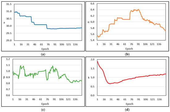
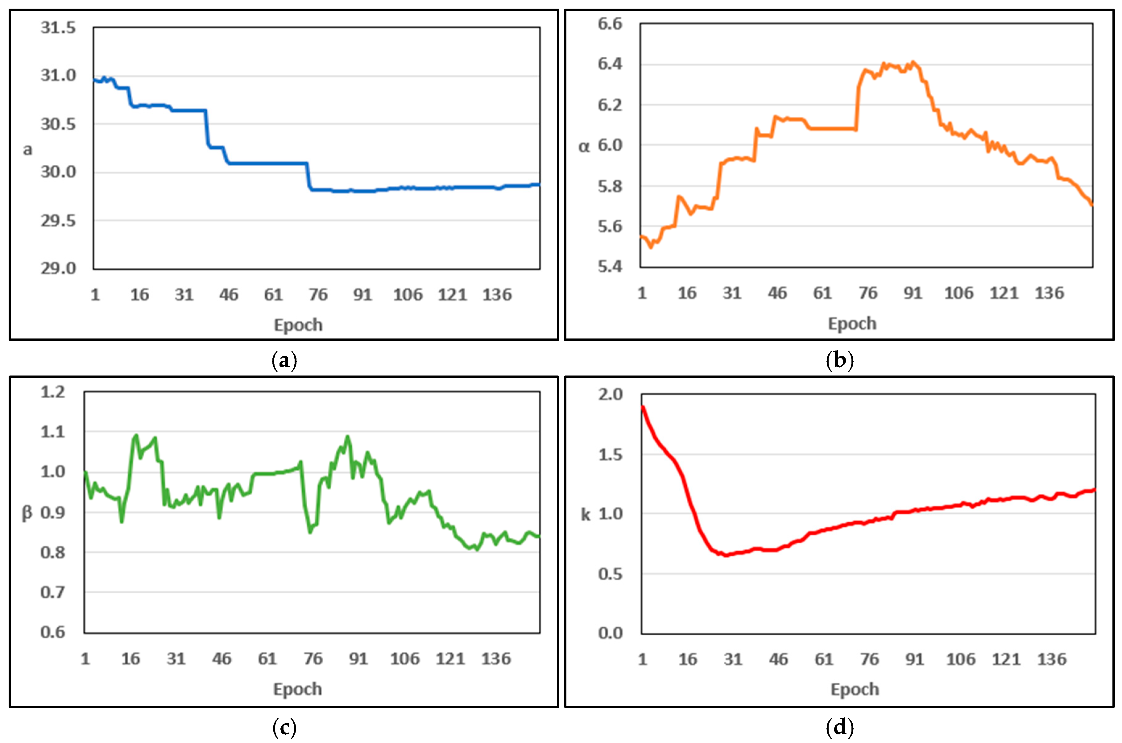
Table 14 presents the parameter estimation results for dataset 3. The parameters estimated by DL-BPE were $\widehat{a}$ = 29.8784, $\widehat{\alpha }$ = 5.7071, $\widehat{\beta }$ = 0.8393, and $\widehat{k}$ = 1.2055. Figure 10 illustrates the changes in each parameter over 150 epochs obtained from the DL-BPE, following the same color described previously. Overall, $a$ decreased and stabilized, $\alpha$ increased and then declined, $\beta$ fluctuated moderately, and $k$ decreased sharply before gradually increasing. The final estimate of $\widehat{\alpha }$ = 5.7071 suggests that the fault-detection behavior in dataset 3 was represented by an increasing and convex pattern.

Table 14. Parameter estimation results of the proposed model for dataset 3.

Method	$\widehat{\mathit{a}}$	$\widehat{\mathit{\alpha }}$	$\widehat{\mathit{\beta }}$	$\widehat{\mathit{k}}$
LSE	30.7429	0.4716	0.0027	0.9476
MLE	39.2220	0.0597	0.000024	0.00000001
DL-BPE	29.8784	5.7071	0.8393	1.2055

Figure 10. Changes in parameter values during DL-BPE training for dataset 3; (a) $a$; (b) $\alpha$; (c) $\beta$; (d) $k.$

Table 15 presents the evaluation criteria calculated based on the estimation results reported in Table 14. For Dataset 3, DL-BPE showed the best overall performance and the lowest preSSE of 4.4320, compared with 8.8437 for MLE and 19.2124 for LSE. Figure 11 shows the differences between the observed and estimated cumulative failure values at each time point for each estimation method. The gray shaded area represents the same 95% Poisson-based interval described for Figure 7, and the differences remained within this interval across most time points. During the test period, DL-BPE maintained smaller prediction errors than LSE and MLE, consistent with its lower preSSE.

Table 15. Results of the criteria between parameter estimation methods from dataset 3.

Method	MSE	PRR	PP	MAE	RMSPE	MEOP	PC	Adj_R2	preSSE
LSE	2.6283	0.1269	0.1180	1.3574	1.5009	1.2860	11.5576	0.9217	19.2124
MLE	1.5648	0.0708	0.0690	1.0106	1.1579	0.9574	6.8906	0.9534	8.8437
DL-BPE	0.7312	0.0242	0.0214	0.6366	0.7885	0.6031	0.0430	0.9782	4.4320

Figure 11. Difference between observed and estimated cumulative failure values for dataset 3.

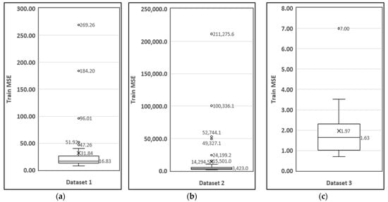
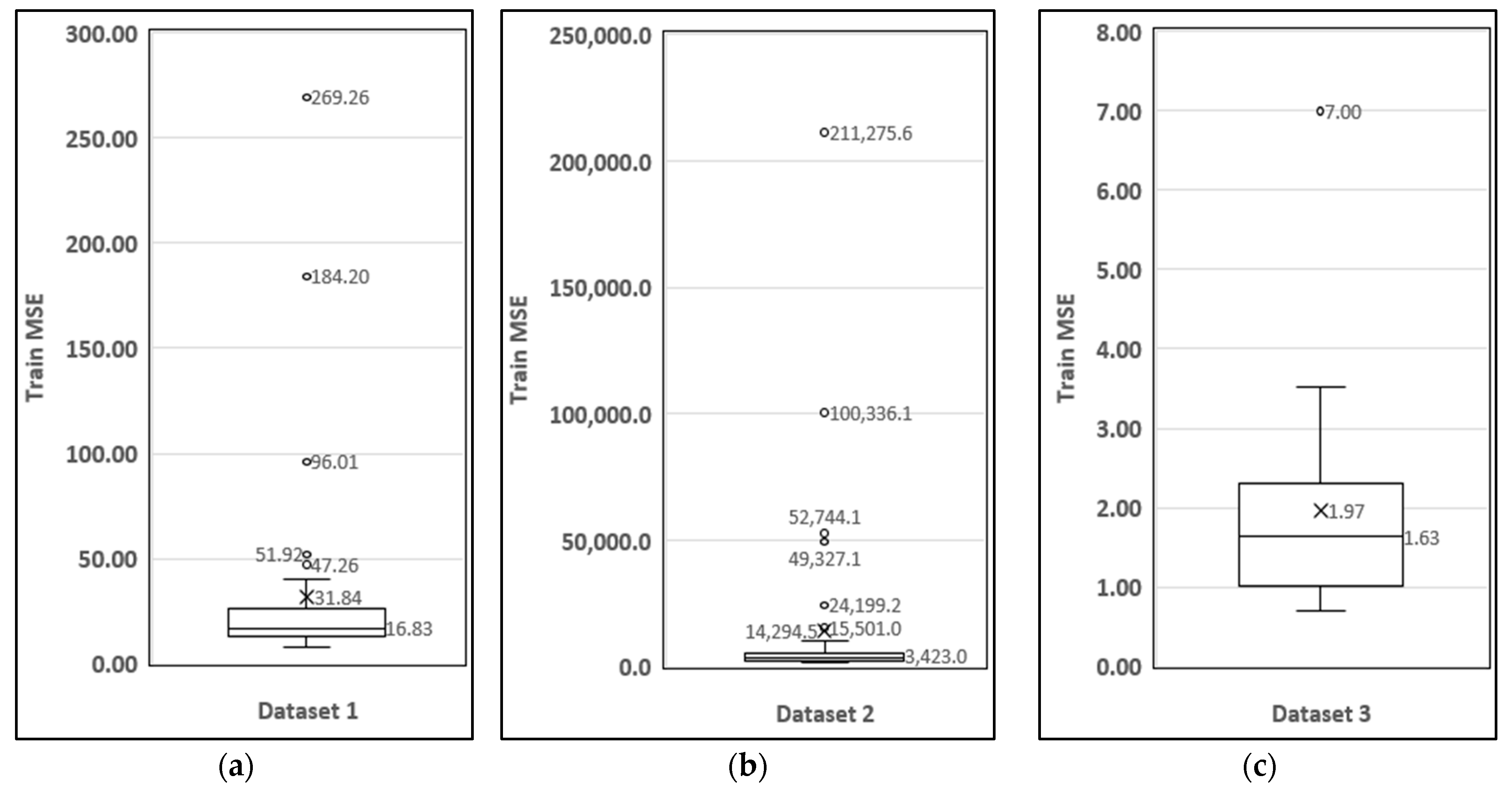
The results from the selected training run are reported together with the distribution across the 40 repeated training runs. To examine the variability of DL-BPE, the model was independently trained 40 times under the same hyperparameter settings, and the distribution of Train MSE was summarized using the mean, standard deviation, median, and quartiles. Table 16 summarizes these descriptive statistics for the three datasets, while Figure 12 illustrates the corresponding Train MSE distributions using boxplots. The x symbols denote the means, the numbers displayed within the boxes indicated the medians, and the circles represent outliers. Due to the stochastic nature of deep learning and its sensitivity to initial weights, several high-error outliers were observed across the repeated training runs. For dataset 1, the Q1 and median MSE values were 13.140 and 16.830, respectively. Although these values were higher than the LSE and MLE results, the selected training run achieved an MSE of 7.5261, outperforming both conventional methods. For dataset 2, the Q1 MSE was 2017.600, which was lower than the MLE MSE of 3124.5981, indicating that at least one-quarter of the DL-BPE runs achieved better performance than MLE. Moreover, the selected training run yielded an MSE of 139.9975, which was substantially lower than those of both LSE and MLE. For dataset 3, the Q1 MSE of 1.020 was lower than both LSE and MLE, while the median MSE of 1.630 was lower than LSE and close to MLE. These results indicate that DL-BPE can achieve competitive in-sample fitting performance in selected runs, although its training performance varies across random initializations. The computational cost was evaluated separately for hyperparameter tuning and repeated training. The computational times for hyperparameter tuning and the subsequent 40 independent training runs were approximately 18.6 and 9.6 min for dataset 1, 30.4 and 10.1 min for dataset 2, and 15.8 and 8.7 min for dataset 3.

Table 16. Descriptive statistics of Train MSE across 40 repeated DL-BPE training runs for the three datasets.

Dataset	Mean	Median	SD	Q1	Q3
Dataset 1	31.8357	16.8324	48.9661	13.1390	25.8258
Dataset 2	14,294.51	3423.019	36,909.65	2017.599	5305.255
Dataset 3	1.9681	1.6322	1.4025	1.0164	2.2801

Figure 12. Boxplots of Train MSE from 40 repeated DL-BPE training runs; (a) dataset 1; (b) dataset 2; (c) dataset 3.

5. Discussion

The proposed convex-dependent NHPP SRM achieved competitive fitting performance across all three datasets. For dataset 1, the proposed model achieved the best results across all eight evaluation criteria. For dataset 2, it performed best for MAE, MEOP, and PC and achieved the second-best results for MSE, RMSPE, and Adj_R². For dataset 3, it also achieved the best results for several major criteria, including MSE, RMSPE, MEOP, PC, and Adj_R². These findings suggest that incorporating convex fault-detection behavior, dependent failures, and a nonzero initial failure state provides a useful extension of conventional NHPP SRMs for representing different software failure patterns.

The predictive performance of DL-BPE relative to LSE and MLE varied across the datasets. The differences among the estimation methods were most pronounced for dataset 2, in which cumulative failures continued to increase substantially during the test period. In this case, the prediction errors of LSE and MLE increased during the later test observations, whereas DL-BPE maintained comparatively smaller deviations from the observed cumulative failures. By contrast, the differences among the methods were less pronounced for datasets 1 and 3, where the test-period failure trajectories were less variable. These results indicate that the relative predictive performance of the estimation methods depends partly on the characteristics of the failure process encountered beyond the training period.

Previous deep-learning studies in software reliability have primarily used neural-network architectures to predict software failures or reliability measures directly. In contrast, DL-BPE uses deep learning as a parameter-estimation framework by embedding the mathematical structure of the proposed NHPP SRM into the network. Its contribution therefore lies not only in predicting future failure behavior but also in estimating the structural parameters of an interpretable reliability model. The 95% Poisson-based intervals further showed that the observed cumulative failure values were generally consistent with the variability implied by the fitted DL-BPE model, including during the test periods. However, the repeated-training results revealed variability across random initializations, particularly for datasets 1 and 2, indicating that the stochastic nature of neural-network optimization should be considered when interpreting a single fitted result.

The proposed framework combines the mathematical interpretability of an NHPP SRM with the flexibility of deep-learning-based parameter estimation. Nevertheless, the evaluation was limited to three benchmark datasets, some of which are relatively old and contain failure information aggregated across software releases or failure categories. The DL-BPE results varied across repeated training runs, and some parameter estimates obtained using LSE and MLE, particularly $\beta$, were close to the lower bounds of the admissible ranges, potentially limiting their direct interpretation. Independent external datasets were also not used for validation. Future research could extend the proposed formulation to more complex failure mechanisms and other NHPP-based SRMs, investigate sequential or online parameter estimation, and validate the framework using more recent industrial and cross-project datasets.

6. Conclusions

This study proposed a convex-dependent NHPP software reliability model that incorporates a Weibull-based fault-detection process, dependent failures, and a nonzero initial failure state. The proposed model was evaluated against existing NHPP SRMs using three software failure datasets and showed competitive fitting performance across different failure patterns. In addition, DL-BPE was introduced as an alternative parameter estimation framework that embeds the mathematical structure of the proposed SRM into a deep-learning architecture.

The empirical results indicate that the proposed SRM provides a useful framework for representing complex software failure processes, while DL-BPE offers a flexible, structurally informed approach to predicting cumulative failures. The predictive results also suggest that the relative performance of the estimation methods depends on the characteristics of the failure process observed beyond the training period. Overall, the study demonstrates the potential of combining an interpretable NHPP-inspired structure with data-driven sequential learning for software reliability modeling.

References

- Ogundipe, O.; Aweto, T. The shaky foundation of global technology: A case study of the 2024 CrowdStrike outage. Int. J. Multidiscip. Res. Growth Eval. 2024, 5, 106–108. [Google Scholar]
- Kumar, P.; Singh, L.K.; Kumar, C. Suitability analysis of software reliability models for its applicability on NPP systems. Qual. Reliab. Eng. Int. 2018, 34, 1491–1509. [Google Scholar] [CrossRef] [Scilit]
- Box, G.E.P.; Jenkins, G.M.; Reinsel, G.C.; Ljung, G.M. Time Series Analysis: Forecasting and Control; John Wiley & Sons: Hoboken, NJ, USA, 2015. [Google Scholar]
- Jelinski, Z.; Moranda, P. Software reliability research. In Statistical Computer Performance Evaluation; Elsevier: Amsterdam, The Netherlands, 1972; pp. 465–484. [Google Scholar] [CrossRef] [Scilit]
- Singpurwalla, N.D.; Wilson, S.P. Software Reliability Modeling. Int. Stat. Rev. 1994, 62, 289. [Google Scholar] [CrossRef] [Scilit]
- Goel, A.L.; Okumoto, K. Time-Dependent Error-Detection Rate Model for Software Reliability and Other Performance Measures. IEEE Trans. Reliab. 1979, R-28, 206–211. [Google Scholar] [CrossRef] [Scilit]
- Yamada, S.; Ohtera, H.; Narihisa, H. Software Reliability Growth Models with Testing-Effort. IEEE Trans. Reliab. 1986, 35, 19–23. [Google Scholar] [CrossRef] [Scilit]
- Yamada, S.; Tokuno, K.; Osaki, S. Imperfect debugging models with fault introduction rate for software reliability assessment. Int. J. Syst. Sci. 1992, 23, 2241–2252. [Google Scholar] [CrossRef] [Scilit]
- Kim, Y.S.; Song, K.Y.; Pham, H.; Chang, I.H. A Software Reliability Model with Dependent Failure and Optimal Release Time. Symmetry 2022, 14, 343. [Google Scholar] [CrossRef] [Scilit]
- Pham, H. A new software reliability model with Vtub-shaped fault-detection rate and the uncertainty of operating environments. Optimization 2014, 63, 1481–1490. [Google Scholar] [CrossRef] [Scilit]
- Kumar, P.; Singh, Y. An empirical study of software reliability prediction using machine learning techniques. Int. J. Syst. Assur. Eng. Manag. 2012, 3, 194–208. [Google Scholar] [CrossRef] [Scilit]
- Jaiswal, A.; Malhotra, R. Software reliability prediction using machine learning techniques. Int. J. Syst. Assur. Eng. Manag. 2018, 9, 230–244. [Google Scholar] [CrossRef] [Scilit]
- Yadav, N.; Yadav, V. Software reliability prediction and optimization using machine learning algorithms: A review. J. Integr. Sci. Technol. 2023, 11, 457. [Google Scholar]
- Zheng, J. Predicting software reliability with neural network ensembles. Expert Syst. Appl. 2009, 36, 2116–2122. [Google Scholar] [CrossRef] [Scilit]
- Ramasamy, S.; Lakshmanan, I. Machine Learning Approach for Software Reliability Growth Modeling with Infinite Testing Effort Function. Math. Probl. Eng. 2017, 2017, 8040346. [Google Scholar] [CrossRef] [Scilit]
- Wu, C.-Y.; Huang, C.-Y. A Study of Incorporation of Deep Learning Into Software Reliability Modeling and Assessment. IEEE Trans. Reliab. 2021, 70, 1621–1640. [Google Scholar] [CrossRef] [Scilit]
- Kim, Y.S.; Pham, H.; Chang, I.H. Deep-Learning Software Reliability Model Using SRGM as Activation Function. Appl. Sci. 2023, 13, 10836. [Google Scholar] [CrossRef] [Scilit]
- Tamura, Y.; Yamada, S. Software Reliability Model Selection Based on Deep Learning with Application to the Optimal Release Problem. J. Ind. Eng. Manag. Sci. 2016, 2016, 43–58. [Google Scholar] [CrossRef] [Scilit]
- Tamura, Y.; Yamada, S. Prototype of 3D Reliability Assessment Tool Based on Deep Learning for Edge OSS Computing. Mathematics 2022, 10, 1572. [Google Scholar] [CrossRef] [Scilit]
- Roy, P.; Mahapatra, G.; Rani, P.; Pandey, S.; Dey, K. Robust feedforward and recurrent neural network based dynamic weighted combination models for software reliability prediction. Appl. Soft Comput. 2014, 22, 629–637. [Google Scholar] [CrossRef] [Scilit]
- Alshehri, W.; Kammoun Jarraya, S.; Allinjawi, A. Software Reliability Prediction Based on Recurrent Neural Network and Ensemble Method. Computers 2024, 13, 335. [Google Scholar] [CrossRef] [Scilit]
- Wang, J.; Zhang, C. Software reliability prediction using a deep learning model based on the RNN encoder–decoder. Reliab. Eng. Syst. Saf. 2018, 170, 73–82. [Google Scholar] [CrossRef] [Scilit]
- Li, C.; Zheng, J.; Okamura, H.; Dohi, T. Software Reliability Prediction through Encoder-Decoder Recurrent Neural Networks. Int. J. Math. Eng. Manag. Sci. 2022, 7, 325–340. [Google Scholar] [CrossRef] [Scilit]
- Oveisi, S.; Moeini, A.; Sayeh, M. LSTM Encoder-Decoder Dropout Model in Software Reliability Prediction. Int. J. Reliab. Risk Saf. Theory Appl. 2021, 4, 1–12. [Google Scholar] [CrossRef] [Scilit]
- Yeh, W.-C.; Forghani-elahabad, M.; Kumar, A. Machine learning based estimation of binary state network reliability under varying data availability. Discov. Artif. Intell. 2026, 6, 623. [Google Scholar] [CrossRef] [Scilit]
- Gupta, R.D.; Kundu, D. Exponentiated Exponential Family: An Alternative to Gamma and Weibull Distributions. Biom. J. 2001, 43, 117–130. [Google Scholar]
- Hossain, S.A.; Dahiya, R.C. Estimating the parameters of a non-homogeneous Poisson-process model for software reliability. IEEE Trans. Reliab. 1993, 42, 604–612. [Google Scholar] [CrossRef] [Scilit]
- Yamada, S.; Ohba, M.; Osaki, S. S-Shaped Reliability Growth Modeling for Software Error Detection. IEEE Trans. Reliab. 1983, R-32, 475–484. [Google Scholar] [CrossRef] [Scilit]
- Osaki, S.; Hatoyama, Y. Inflexion S-shaped software reliability growth model. In Stochastic Models in Reliability Theory; Springer: Berlin/Heidelberg, Germany, 1984; pp. 144–162. [Google Scholar] [CrossRef] [Scilit]
- Roy, P.; Mahapatra, G.S.; Dey, K.N. An NHPP software reliability growth model with imperfect debugging and error generation. Int. J. Reliab. Qual. Saf. Eng. 2014, 21, 1450008. [Google Scholar] [CrossRef] [Scilit]
- Kapur, P.K.; Pham, H.; Anand, S.; Yadav, K. A Unified Approach for Developing Software Reliability Growth Models in the Presence of Imperfect Debugging and Error Generation. IEEE Trans. Reliab. 2011, 60, 331–340. [Google Scholar] [CrossRef] [Scilit]
- Lee, D.H.; Chang, I.H.; Pham, H. Software Reliability Model with Dependent Failures and SPRT. Mathematics 2020, 8, 1366. [Google Scholar] [CrossRef] [Scilit]
- Ishii, T.; Dohi, T.; Okamura, H. Software Reliability Prediction Based on Least Squares Estimation. Qual. Technol. Quant. Manag. 2012, 9, 243–264. [Google Scholar] [CrossRef] [Scilit]
- Bae, H.J. Performance Assessment of NHPP Software Reliability Models Applying PARETO-type Lifetime Distribution Properties. J. Theor. Appl. Inf. Technol. 2025, 103, 2857–2867. [Google Scholar] [CrossRef]
- Zhang, H.; Zhang, J.; Shi, K.; Wang, H. Applying Software Metrics to RNN for Early Reliability Evaluation. J. Control Sci. Eng. 2020, 2020, 8814394. [Google Scholar] [CrossRef] [Scilit]
- San, K.K.; Washizaki, H.; Fukazawa, Y.; Honda, K.; Taga, M.; Matsuzaki, A. Deep Cross-Project Software Reliability Growth Model Using Project Similarity-Based Clustering. Mathematics 2021, 9, 2945. [Google Scholar] [CrossRef] [Scilit]
- Samek, W.; Montavon, G.; Lapuschkin, S.; Anders, C.J.; Muller, K.-R. Explaining deep neural networks and beyond: A review of methods and applications. Proc. IEEE 2021, 109, 247–278. [Google Scholar] [CrossRef] [Scilit]
- de Amorim, L.B.V.; Cavalcanti, G.D.C.; Cruz, R.M.O. The choice of scaling technique matters for classification performance. Appl. Soft Comput. 2023, 133, 109924. [Google Scholar] [CrossRef] [Scilit]
- Perronnin, F.; Sánchez, J.; Mensink, T. Improving the fisher kernel for large-scale image classification. In European Conference on Computer Vision, 2010; Springer: Berlin/Heidelberg, Germany, 2010; pp. 143–156. [Google Scholar] [CrossRef] [Scilit]
- Misra, P.N. Software reliability analysis. IBM Syst. J. 1983, 22, 262–270. [Google Scholar] [CrossRef] [Scilit]
- Singh, V.B.; Sharma, M. Prediction of the Complexity of Code Changes Based on Number of Open bugs, New Feature and Feature Improvement. In 2014 IEEE International Symposium on Software Reliability Engineering Workshops; IEEE: Piscataway, NJ, USA, 2014; pp. 478–483. [Google Scholar] [CrossRef] [Scilit]
- Sahinoglu, M.; Can, Ü. Alternative Parameter Estimation Methods for the Compound Poisson Software Reliability Model with Clustered Failure Data. Softw. Test. Verif. Reliab. 1997, 7, 35–57. [Google Scholar]
- Pham, H. An imperfect-debugging fault-detection dependent-parameter software. Int. J. Autom. Comput. 2007, 4, 325–328. [Google Scholar] [CrossRef] [Scilit]
- Sharma, K.; Garg, R.; Nagpal, C.K.; Garg, R.K. Selection of Optimal Software Reliability Growth Models Using a Distance Based Approach. IEEE Trans. Reliab. 2010, 59, 266–276. [Google Scholar] [CrossRef] [Scilit]
- Pham, H. On Estimating the Number of Deaths Related to Covid-19. Mathematics 2020, 8, 655. [Google Scholar] [CrossRef] [Scilit]
- Chiu, K.-C.; Huang, Y.-S.; Lee, T.-Z. A study of software reliability growth from the perspective of learning effects. Reliab. Eng. Syst. Saf. 2008, 93, 1410–1421. [Google Scholar] [CrossRef] [Scilit]
- Bergmeir, C.; Benítez, J.M. On the use of cross-validation for time series predictor evaluation. Inf. Sci. 2012, 191, 192–213. [Google Scholar] [CrossRef] [Scilit]
- Fadhilah, N.A.; Rizki, M.A.D.; Azahran, M.R.; Arbaynah, S.; Yusuf, R.P.A.; Angraini, Y.; Nurhambali, M.R. Long Short-Term Memory as a Rainfall Forecasting Model for Bogor City in 2025–2026. J. Appl. Inform. Comput. 2025, 9, 333–340. [Google Scholar] [CrossRef] [Scilit]
- Bischl, B.; Binder, M.; Lang, M.; Pielok, T.; Richter, J.; Coors, S.; Thomas, J.; Ullmann, T.; Becker, M.; Boulesteix, A.; et al. Hyperparameter optimization: Foundations, algorithms, best practices, and open challenges. Wiley Interdiscip. Rev. Data Min. Knowl. Discov. 2023, 13, e1484. [Google Scholar] [CrossRef] [Scilit]
Disclaimer/Publisher’s Note: The statements, opinions and data contained in all publications are solely those of the individual author(s) and contributor(s) and not of MDPI and/or the editor(s). MDPI and/or the editor(s) disclaim responsibility for any injury to people or property resulting from any ideas, methods, instructions or products referred to in the content. |
© 2026 by the authors. Licensee MDPI, Basel, Switzerland. This article is an open access article distributed under the terms and conditions of the Creative Commons Attribution (CC BY) license.