


Abstract
Full-vehicle active suspension control requires coordinated regulation of ride comfort, body posture, suspension travel, tire road holding, and control effort. To improve the adaptability of fixed-weight MPC while retaining model-based interpretability, this paper proposes a TD3-MPC posture-feedback controller for a seven-degree-of-freedom full-vehicle active suspension system. The TD3 Actor is trained offline and deployed with fixed network parameters to generate five bounded actions for online MPC weight regulation rather than directly outputting actuator forces. The MPC layer calculates the constrained four-wheel baseline forces, after which posture feedback compensates for vehicle-body vertical, pitch, and roll responses. A composite reward balances body acceleration, suspension deflection, tire deformation, energy control, force variation, and action smoothness. The controller is evaluated through time-domain, frequency-domain, parameter-perturbation, ablation, and Monte Carlo analyses. Under the nominal Class-D Road condition at 20 m/s, it reduced the RMS values of body vertical, pitch, and roll angular accelerations by 13.24%, 4.77%, and 10.68%, respectively, and reduced control energy by 3.06% relative to fixed-weight MPC. Across 360 paired cases covering ISO Class-B-D roads and speeds of 10–25 m/s, the corresponding mean reductions were 9.55%, 6.30%, and 8.37%, respectively.
Keywords:
full-vehicle active suspension; model predictive control; TD3; multi-objective optimization; posture feedback; vehicle dynamics MSC:
93B45; 93E35; 93C40
1. Introduction
Active suspension control is a constrained multi-objective problem in vehicle dynamics. It must attenuate vehicle-body vibration, suppress pitch and roll motions, maintain suspension working space, reduce tire-load variation, and limit actuator energy consumption simultaneously [1,2]. These objectives are strongly coupled under stochastic road excitation; therefore, the controller should balance ride comfort, road holding, actuator feasibility, and vehicle-body posture stability [3,4,5,6,7].
Model predictive control (MPC) is suitable for active and semi-active suspension systems because it can handle multi-objective optimization and physical constraints within a finite-horizon framework [4,5,6,8,9,10,11,12]. Existing studies have introduced preview information, event-triggered computation, explicit MPC, actuator-oriented MPC, and adaptive weighting strategies to improve suspension performance [7,13,14,15]. However, conventional MPC usually relies on weighting matrices tuned offline. A fixed weight set may not maintain an appropriate trade-off among comfort, posture stability, suspension deflection, tire deformation, and control effort when road excitation, vehicle speed, or operating state changes [16,17,18].
Deep reinforcement learning (DRL) provides a data-driven way to improve adaptability in nonlinear and time-varying suspension-control problems. Recent studies have applied DDPG, TD3, PPO, and safety-constrained DRL to active or semi-active suspension systems [15,16,17]. Nevertheless, using DRL as an end-to-end force controller may produce abrupt or unsafe actuator commands, and it is difficult to explicitly guarantee actuator saturation, suspension travel, tire-load constraints, and control interpretability [19,20]. Thus, this study does not use DRL to directly output actuator forces.
TD3 is selected because the proposed tuning task requires continuous bounded actions for MPC weight regulation. Compared with DDPG, TD3 uses clipped double-Q learning, delayed policy updates, and smoothing target-policy to reduce value overestimation and improve training stability [21]. Compared with value-iteration-based online reinforcement learning for unknown multi-agent systems, the present method has a different objective: TD3 is used to adjust MPC weighting parameters rather than to learn a complete low-level control law [19,20,22,23]. This design is consistent with RL-MPC studies where MPC is retained as a safety or constraint-handling layer and learning improves adaptability [24,25,26,27].
Based on this motivation, this paper proposes a TD3-MPC posture-feedback control strategy for a full-vehicle active suspension system [28]. The TD3 agent outputs five bound continuous actions to regulate MPC weights, the MPC layer solves the constrained finite-horizon optimization problem to obtain four-wheel base active forces, and the posture-feedback module compensates for vehicle-body heave, pitch, and roll motions. The proposed method is evaluated against passive suspension and fixed-weight MPC under stochastic road excitation, parameter perturbations, and ablation conditions.
The remainder of this paper is organized as follows. Section 2 establishes full-vehicle suspension and stochastic road models. Section 3 presents the TD3-MPC posture-feedback framework, including observation input, action output, weight regulation, MPC optimization, posture feedback, and reward design. Section 4 analyzes adaptive-weight boundedness, recursive feasibility, practical stability, and TD3 training convergence. Section 5 reports time-domain, frequency-domain, robustness, and ablation results. Section 6 concludes the paper.
2. Full-Vehicle Active Suspension and Road Excitation Modeling
This section establishes the full-vehicle model used for controller design. The coupled heave, pitch, roll, and unsprung-mass dynamics are first described, followed by the state-space representation and the stochastic road-input model based on ISO 8608.
2.1. Seven-Degree-of-Freedom Full-Vehicle Active Suspension Model
A seven-degree-of-freedom full-vehicle active suspension model is adopted in this paper. The seven degrees of freedom include vehicle-body vertical motion, vehicle-body pitch motion, vehicle-body roll motion, and the vertical motions of the left-front, right-front, left-rear, and right-rear unsprung masses [29,30]. A four-wheel configuration is adopted because it represents the standard full-vehicle architecture of passenger vehicles and is the minimum model capable of describing the coupled heave, pitch, roll, and four independent unsprung-mass motions. It is also consistent with the four-corner actuator configuration considered in this study. Multi-axle buses and trucks can be modeled by augmenting the unsprung-mass coordinates, road inputs, and actuator-force vector, but such extensions are beyond the present scope.
The full-vehicle state variables are defined as:
where denotes the vertical displacement of the vehicle-body mass center, denotes the vertical velocity of the vehicle-body mass center; and denote the vehicle-body pitch angle and pitch angular velocity; and denote the vehicle-body roll angle and roll angular velocity; , , , and are the vertical displacements of the left-front, right-front, left-rear, and right-rear unsprung masses, respectively.
The vertical displacements of the four body corners can be obtained from the vertical displacement of the vehicle-body mass center, the pitch angle, and the roll angle:
where denotes the vertical displacement at the suspension mounting point of the vehicle body; denotes the distance from the vehicle mass center to the front axle; denotes the distance from the vehicle mass center to the rear axle; denotes the front track width, and denotes the rear track width, respectively.
The four-wheel suspension dynamic deflection is defined as:
where denotes the dynamic deflection of the suspension.
The four-wheel tire deformation is defined as:
where denotes the vertical deformation of the tire, and denotes the road input corresponding to the wheel.
The preceding dynamic equations establish the generalized coordinates and tire-road excitation variables of the seven-degree-of-freedom vehicle model. To clarify the spatial relationship among the sprung mass, four unsprung masses, suspension elements, tire elements, and road inputs, the corresponding full-vehicle active suspension schematic is shown in Figure 1.
Figure 1.
Schematic Diagram of the Seven-Degree-of-Freedom Full-Vehicle Active Suspension.
2.2. Suspension Force, Tire Force, and State-Space Representation
The vehicle model is derived using Newton-Euler force and moment equilibrium. The sprung body is regarded as a rigid body with small pitch and roll angles, while each unsprung mass is described by its vertical force equilibrium. The suspension and tire elements are represented by linear spring-damper and linear elastic relationships, respectively [29,30,31,32,33,34].
The passive spring-damping force of the suspension is expressed as [30,32,33,34]:
where denotes the spring-damping force of the suspension; and denote suspension stiffness and suspension damping.
The dynamic-load-related force of the tire is expressed as:
where denotes the vertical elastic force of the tire, and denotes the tire stiffness.
The four-wheel active suspension control-force vector is defined as:
where , , and denote the control forces output by the left-front, right-front, left-rear, and right-rear active suspension actuators at the kth control instant.
The vehicle-body vertical dynamic equation is:
where denotes the sprung mass of the vehicle body and denotes the vertical acceleration of the vehicle body.
The vehicle-body pitch dynamic equation is:
where denotes the pitch moment of inertia of the vehicle body around the lateral axis and denotes the pitch angular acceleration of the vehicle body.
The vehicle-body roll dynamic equation is:
where denotes the roll moment of inertia of the vehicle body around the longitudinal axis and denotes the roll angular acceleration of the vehicle body.
The dynamic equations of the four unsprung masses are:
where denotes the unsprung mass and denotes the vertical acceleration of the unsprung mass.
The above full-vehicle dynamic equations are arranged into the continuous state-space form:
where denotes the continuous state matrix; denotes the active control-force input matrix; denotes the road input matrix; denotes the output matrix; denotes the direct transmission matrices from control force and denotes road input to the output.
The continuous model is discretized using the sampling time to obtain:
where denotes the state vector at the denotes sampling instant, denotes the four-wheel active control-force vector, denotes the four-wheel road input vector, denotes the performance output vector, and , , , , , denote the discretized system matrices. Equations (12)–(14) define the continuous-time state-space model, its discrete-time representation, and the performance-output vector, respectively. The explicit matrix forms corresponding to the state ordering in Equation (1), including and their discrete-time counterparts, are provided in Appendix B.
The performance output vector is selected as:
where the first three terms are used to evaluate vehicle-body comfort and posture stability, the four suspension dynamic deflections are used to evaluate suspension safety travel, and the four tire deformations are used to evaluate tire road-holding performance.
The body vertical acceleration is evaluated at the sprung-mass center, while the pitch and roll angular accelerations correspond to rotations about the lateral and longitudinal axes through the same center. Suspension dynamic deflections are evaluated between the sprung and unsprung mounting points at the four vehicle corners, and tire deformations are evaluated at the four wheel-road interfaces. In practical implementation, these quantities can be obtained using body-mounted IMU, suspension-displacement sensors, and wheel or tire-state estimators.
2.3. Random Road Input Model
The road-roughness description follows ISO 8608:2016 [35], in which road classes are defined using the spatial power spectral density . With and the spatial-to-temporal transformation determined by vehicle speed, the corresponding first-order shaping filter leads to Equation (15). The values of for Classes B-D are selected according to the ISO road-quality classification.
In this paper, a first-order filtered white-noise model is used to generate random road inputs [5,17]. The front-wheel road input can be expressed as:
where denotes the front-wheel road input, denotes road lower cut-off frequency, denotes sampling time, denotes road roughness coefficient at the reference spatial frequency , denotes vehicle driving speed, and denotes Gaussian white noise with zero mean and unit variance.
Considering the time delay between the front and rear axles, the rear-wheel road input is:
where denotes the delay step number between front-wheel and rear-wheel road inputs, and its calculation formula is:
The four-wheel road input vector is defined as:
Figure 2 presents one representative D-class road realization used for the nominal time-domain analysis. The D-class road was selected as the nominal excitation because its relatively high roughness provides a demanding condition for examining vibration attenuation, actuator constraints, and multi-objective performance trade-offs. However, a single D-class road realization is not regarded as sufficient evidence of controller robustness or generalizability. Therefore, additional Monte Carlo simulations covering ISO road grades B, C, and D and vehicle speeds of 10, 15, 20, and 25 m/s are conducted in Section 5.6. For each operating condition, the front-wheel road excitation is generated using Equation (15) with the corresponding road roughness coefficient, while the rear-wheel excitation is obtained through the speed-dependent spatial delay defined in Equations (16) and (17). Identical road realizations are applied to all controllers to ensure paired and fair comparisons.
Figure 2.
Class D Random Road Surface Input Diagram.
3. TD3-MPC Posture-Feedback Control Strategy
This section presents the proposed TD3-MPC posture-feedback control strategy. It describes the TD3 observation and action spaces, the mapping from bounded actions to MPC weights, the constrained calculation of four-wheel control forces, the posture-feedback compensation, and the offline TD3 training mechanism.
3.1. TD3 Agent Observation Input and Overall Control Architecture
At the reinforcement-learning decision instant, the TD3 agent receives a history-augmented observation vector defined as
where denotes the observation input of the TD3 agent, denotes the mean value of four-wheel suspension dynamic deflection, denotes the maximum value of four-wheel suspension dynamic deflection, denotes the mean value of four-wheel tire deformation, denotes the maximum value of four-wheel tire deformation, denotes the maximum allowable output force of the actuator, and denotes the action vector output by TD3 at the previous instant. The normalized previous control forces and the previous TD3 action are included to provide short-term control memory for adaptive weight regulation.
The mean value of four-wheel suspension dynamic deflection is defined as:
The mean value of four-wheel tire deformation is defined as:
The observation vector in (19) is constructed from measurable vehicle responses and historical control information rather than from the full physical state of the suspension system. Accordingly, the proposed reinforcement-learning formulation is implemented as an observation-based, history-augmented control problem. The road excitation and the vehicle speed are embedded in the full-vehicle environment and road-delay model; their influence is reflected in the measured response components contained in Vehicle speed is not included as an independent component of the TD3 observation vector . Nevertheless, it is not neglected in the closed-loop control framework. As an exogenous operating parameter, explicitly enters the stochastic road model in Equation (15) and determines the front-rear road-input delay through Equation (17). Consequently, variations in vehicle speed change both the temporal characteristics of the road excitation and the phase relationship between the front- and rear-wheel inputs. These effects propagate through the full-vehicle dynamics and are reflected in the body accelerations, suspension dynamic deflections, tire deformations, and historical control information contained in .
Therefore, the TD3 actor employs a response-driven weight-regulation mechanism rather than a speed-scheduled mechanism. This design reduces the observation dimension and enables the controller to regulate the MPC weights according to the actual dynamic consequences of changes in vehicle speed and road excitation. Its effectiveness over the investigated speed range is further evaluated through the multi-speed Monte Carlo simulations presented in Section 5.6. However, the current validation considers constant vehicle speed within each simulation case; directly incorporating into may improve adaptation during rapid speed transitions and will be investigated in future work.
Based on , the TD3 Actor outputs a continuous action vector , which is then mapped to the MPC weighting parameters. The MPC layer subsequently solves the constrained finite-horizon optimization problem to obtain the four-wheel base control force . The posture-feedback module then compensates for the vehicle-body heave, pitch, and roll motions, and the final control force is obtained after saturation processing. The resulting information flow can be summarized as
The overall control architecture of the proposed TD3-MPC posture-feedback strategy and the interaction between the TD3 agent and the full-vehicle suspension environment are illustrated in Figure 3.
Figure 3.
Overall Control Framework of the TD3-MPC Posture-Feedback Strategy.
3.2. Continuous Action Output of the Actor Network
The Actor policy network in the TD3 agent outputs a continuous action vector according to the observation input:
where denotes the continuous action vector output by the Actor network at the decision instant, denotes the deterministic policy function, and denotes the Actor network parameters.
In this paper, a five-dimensional continuous action is set as:
where , , , and are used to adjust the vehicle-body vertical acceleration weight, the vehicle-body pitch angular acceleration weight, the vehicle-body roll angular acceleration weight, the weights related to suspension dynamic deflection and tire deformation, and the control energy-consumption weight, respectively.
The output layer of the Actor network adopts the hyperbolic tangent function, so that the action is limited within a specified range :
where denotes the hidden-layer features of the Actor network;
denotes the hyperbolic tangent activation function, which maps the raw Actor output into the bounded interval
. This bounded output is then used for MPC weight regulation, thereby preventing the TD3 action from generating weighting coefficients outside the prescribed range;
and
denote the output-layer weighting matrix and bias vector, respectively.
3.3. Action-to-Weight Mapping for Adaptive MPC
To convert the normalized actions output by TD3 into MPC weight scaling coefficients, a linear mapping is adopted:
where denotes the scaling coefficient of the type of weight at the instant; and denote the lower and upper bounds of this scaling coefficient.
The updated MPC weight can be expressed as:
where denotes the MPC weight at the instant, and denotes the corresponding basic weight.
It should be noted that the TD3 agent does not modify the prediction model, the prediction horizon, or the physical constraint sets of the MPC controller. The online adaptation only changes the relative weighting coefficients in the MPC cost function through the bounded action-to-weight mapping. Therefore, the constrained optimization structure of the MPC problem is preserved during online weight regulation. In addition, since each TD3 action is clipped by the hyperbolic tangent function and then mapped into a prescribed finite interval, the updated weighting matrices remain bounded and positive semidefinite or positive definite. This bounded mapping prevents the MPC weighting matrices from becoming singular, indefinite, or unbounded. Uniform strict convexity and an upper bound on the Hessian condition number are established in Section 4.2.
The connection between the learning layer and the optimization layer is the continuous action-to-weight mapping. Figure 4 illustrates this interface, emphasizing that TD3 adjusts the MPC weighting parameters rather than directly outputting actuator forces.
Figure 4.
TD3 Action-to-MPC Weight Mapping Diagram.
To enhance the optimization ability for vehicle-body acceleration while avoiding obvious deterioration of suspension dynamic deflection and tire deformation, different adjustment ranges are set for different weights in this paper:
where and denote the scaling ranges for vehicle-body acceleration weights, and denote suspension dynamic deflection and tire deformation weights, and and denote control energy-consumption weights, respectively. The numerical values of the baseline MPC weights and the prescribed action-to-weight scaling intervals are provided in Appendix A, Table A1.
3.4. MPC-Based Four-Wheel Active Force Optimization
This subsection formulates the constrained MPC problem used to calculate the four-wheel MPC control-force vector. The prediction model, objective function, and physical constraints are presented in the following subsections.
3.4.1. MPC Prediction Model
Based on the discrete state-space model, state prediction is carried out within the prediction horizon :
where denotes the predicted state at instant obtained at the instant, denotes the control input at the instant within the prediction horizon, and denotes the predicted road input.
The predicted output is:
3.4.2. MPC Objective Function
The MPC optimization objective function at the control instant is defined as [36,37,38]:
where denotes the prediction-horizon length, denotes the control-horizon length, denotes the output weighting matrix adjusted by TD3, denotes the control-input weighting matrix, denotes the control-increment weighting matrix, and denotes the control-input increment.
The updated output weighting matrix is defined as:
where , , denote the weights of vehicle-body vertical acceleration, pitch angular acceleration, and roll angular acceleration, respectively, and denotes the weight related to suspension dynamic deflection and tire deformation.
The control-input weighting matrix is defined as:
where denotes the control of energy-consumption weight and denotes the fourth-order identity matrix.
3.4.3. Constraints
The actuator output-force constraint of the active suspension is:
The suspension dynamic-deflection constraint is:
The tire-deformation constraint is:
where , denote the lower and upper bounds of actuator output force, denotes the allowable limit of suspension dynamic deflection, and denotes and the allowable limit of tire deformation.
The MPC optimization problem is expressed as:
where denotes the control-input sequence within the prediction horizon and denotes the optimal control sequence.
MPC applies the first control quantity to obtain the four-wheel basic active control force:
where denotes the four-wheel basic active control-force vector solved by MPC at the control instant.
3.5. Posture-Feedback Force Compensation
To further suppress the vertical, pitch, and roll posture errors of the vehicle body, posture feedback compensation is added after the MPC basic control force.
The generalized feedback force of the vehicle body is defined as:
where denotes the vehicle-body vertical feedback force, denotes pitch feedback moment, and denotes roll feedback moment.
The feedback law is defined as:
where , denote the vehicle-body vertical feedback gains, , denote pitch feedback gains, and , denote roll feedback gains.
The four-wheel feedback compensation-force vector is defined as:
The relationship between the generalized force and the four-wheel feedback compensation forces satisfies:
where denotes the mapping matrix from four-wheel forces to vehicle-body generalized forces.
The four-wheel feedback compensation forces can be obtained through generalized inverse allocation:
The final four-wheel active control force is:
where denotes the actuator output saturation function.
3.6. Reward Function and TD3 Update Mechanism
This subsection establishes the reward formulation and TD3 update mechanism. Section 3.6.1 defines the single-step cost and its associated reward, whereas Section 3.6.2 presents the Critic and Actor update equations.
3.6.1. Single-Step Cost Function
The reward function in this paper is based on a multi-objective cost function, comprehensively considering vehicle-body comfort, posture stability, suspension safety travel, tire road-holding performance, control energy consumption, control-force change rate, and action smoothness [20,22,23].
The single-step cost function is defined as:
where , , denote the penalty weights of vehicle-body vertical acceleration, pitch angular acceleration, and roll angular acceleration, denotes the penalty weight of suspension dynamic deflection, denotes the penalty weight of tire deformation, denotes the penalty weight of control energy consumption, denotes the penalty weight of control-force change rate, denotes the penalty weight of TD3 action amplitude, and denotes the over-limit penalty weight.
The over-limit penalty of suspension dynamic deflection and tire deformation is defined as:
The reward function is defined as:
where denotes the reward value at the instant. The smaller the cost function is, the larger the reward value is, and the more the agent tends to select the corresponding MPC weight-adjustment action.
The TD3 reward function and the MPC objective function have different but coordinated roles. The MPC objective defines the finite-horizon optimization problem of the lower-level controller, whereas the TD3 reward evaluates the long-term closed-loop consequences of selecting different MPC weights. Therefore, TD3 does not directly minimize the instantaneous MPC objective; instead, it learns an observation-dependent policy for balancing its individual performance terms.
The physical components of the reward are explicitly aligned with the MPC control objectives. The penalties associated with body vertical, pitch, and roll accelerations correspond to the MPC weights , , and , respectively. The suspension-deflection and tire-deformation penalties correspond to the safety-related output weights regulated by the fourth TD3 action, while the control-force penalty corresponds to . The control-force variation and action-amplitude penalties are additionally introduced to discourage abrupt force commands and excessive weight variation. The over-limit penalty increases the cost when the suspension-deflection or tire-deformation limits are approached or exceeded.
Safety and constraint handling do not rely exclusively on the learned reward. The TD3 Actor cannot directly generate actuator forces, and its actions are restricted by the bounded action-to-weight mapping. The resulting control force is computed by the constrained MPC layer and subsequently limited by actuator saturation. Therefore, an imperfect reward may affect the achieved multi-objective trade-off, but it cannot arbitrarily change the MPC prediction model, physical constraints, or prescribed weight intervals.
Nevertheless, the selected reward function is not claimed to provide a universal representation of all real-world driving objectives. Its consistency with the intended control objectives is evaluated empirically through the ablation, parameter-perturbation, and multi-condition Monte Carlo simulations presented in Section 5.
3.6.2. TD3 State-Action Value Function
TD3 uses two Critic networks to estimate the state-action value function:
where , denote the two Critic networks and , denote their network parameters.
Smoothing noise is added to the target action:
where denotes the target Actor network, denotes the parameters of the target Actor network, and denotes the target-action smoothing noise.
The target Q value is defined as:
where denotes the discount factor and denotes the target Critic network. Using the smaller value of the two Critic networks can reduce the overestimation problem of the value function.
The loss function of the Critic network is:
where denotes the batch size of experience replay.
The Actor network is updated through the deterministic policy gradient:
The target networks adopt soft update:
where denotes the soft-update coefficient of the target network.
The TD3 policy and value networks are updated through interaction, replay sampling, target-policy smoothing, double-Critic learning, delayed Actor updating, and soft target updating. The simplified training sequence is presented in Figure 5.
Figure 5.
TD3 Training Update Flowchart.
4. Stability Analysis and Empirical Assessment of TD3 Training
This section analyzes the theoretical properties of the proposed TD3-MPC posture feedback active suspension control method from four aspects: weight boundedness, MPC recursive feasibility, closed-loop input-to-state stability, and TD3 training convergence [39,40,41].
It should be noted that, because the full-vehicle active suspension system contains nonlinear road disturbances, reinforcement-learning approximation errors, and actuator constraints, this paper does not claim that the deep reinforcement-learning policy has strict global optimal convergence. Instead, under standard assumptions, its boundedness, recursive feasibility, practical stability, and policy-iteration convergence trend are analyzed.
4.1. Basic Assumptions
For the convenience of analysis, the following assumptions are given.
Assumption 1.
The discrete full-vehicle active suspension system
is stabilizable; that is, there exists a feedback gain
such that
is a Schur stable matrix.
Assumption 2.
The road input is bounded, that is, there exists a constant such that
where denotes the upper bound of the road input amplitude.
Assumption 3.
The control force of the active suspension actuator is subject to saturation constraints:
Assumption 4.
After the TD3 output action passes through the activation function and linear mapping, the MPC weight scaling coefficient satisfies:
Assumption 5.
The MPC optimization problem is feasible at the initial instant, and the prediction horizon and control constraint sets are reasonably selected so that there exists at least one control sequence satisfying the control-force saturation constraint, suspension dynamic-deflection constraint, and tire-deformation constraint.
4.2. Boundedness of MPC Weights Under TD3 Weight Adjustment
The TD3 agent outputs a five-dimensional continuous action:
The Actor network output layer adopts a hyperbolic tangent function; therefore:
The action is mapped into the MPC weight scaling coefficient:
Since holds, it necessarily follows that:
The MPC weight is:
where denotes the basic weight. Therefore:
It can be seen that, although the TD3 agent can adaptively adjust MPC weights, all weights are always located within preset bounded intervals, and problems such as zero weights, excessively large weights, or objective-function degeneration will not occur. Therefore, the output weighting matrix and control-input weighting matrix in the MPC optimization problem always maintain positive-definite or positive-semidefinite structures.
The updated output weighting matrix is:
The control-input weighting matrix is:
Therefore, there exist constants
,
,
,
such that:
Proposition 1.
For every bounded TD3 action
, the resulting MPC quadratic programming problem remains uniformly strictly convex, and its Hessian condition number is bounded.
Let denote the lifted input-to-output prediction matrix and define
The MPC objective function can be written in the standard quadratic form
where, up to an irrelevant positive scalar factor,
From the bounded action-to-weight mapping, there exist constants , , and such that
Therefore,
It follows that for every admissible TD3 action. Hence, the MPC optimization problem remains strictly convex and possesses a unique minimizer. Moreover,
Thus, bounded action-to-weight mapping cannot cause loss of convexity or an unbounded deterioration of the Hessian conditioning. This result concerns the well-posedness of the quadratic program; conditional feasibility and practical closed-loop stability are discussed separately in Section 4.3 and Section 4.4.
Consequently, the online variation of MPC weights induced by the trained TD3 Actor does not change the feasible set of the MPC optimization problem. It only changes the trade-off among the output-tracking, suspension-deflection, tire-deformation, and control-effort terms. Therefore, the feasibility of the constrained MPC problem can still be analyzed based on the original constraint sets.
4.3. Feasibility Preservation Under Online Weight Regulation
At the control instant, MPC solves the following finite-horizon optimization problem:
where denotes the optimal control sequence obtained at the instant:
MPC actually applies the first control quantity:
At the next instant , a candidate control sequence can be constructed as:
where denotes the stabilizing feedback gain. If this candidate sequence satisfies the constraints of control force, suspension dynamic deflection, and tire deformation, then the MPC optimization problem at that instant has at least one feasible solution. Therefore, recursive feasibility at the next sampling instant is conditional on the shifted optimal sequence remaining admissible under the realized road excitation and actuator constraints. Initial feasibility and bounded road excitation alone do not constitute a general proof of recursive feasibility. Since an explicit robust terminal invariant set is not implemented in the present controller, the analysis establishes feasibility preservation with respect to bounded MPC-weight variation rather than unconditional recursive feasibility under arbitrary operating conditions.
4.4. Analysis of Closed-Loop Practical Stability
The MPC optimal cost function is used as a Lyapunov candidate function for the constrained MPC layer. Since the MPC weights are regulated online by the trained TD3 Actor, the optimal value function is written as
where denotes the optimal objective-function value of the MPC optimization problem at the instant, is the full-vehicle state, and is the MPC weight vector after TD3 regulation.
At the instant, the optimal MPC control sequence is denoted by . The first element of this sequence is the optimal MPC base control force, namely
The corresponding predicted state is induced by the optimal MPC input and the road input. For the discrete full-vehicle model, it can be expressed as
In the disturbance-free case with exact MPC optimization, the standard decrease condition can be written as
Because is positive semidefinite and is positive definite, there exist positive constants and such that the practical Lyapunov difference can be bounded by
where and are positive constants associated with the MPC weighting matrices and the vehicle model. Here, represents the residual term induced by numerical optimization error, bounded weight variation, and model mismatch.
In numerical implementation, the obtained MPC base force may deviate from the ideal optimum because of solver tolerance, fallback handling, and real-time computation limits. Therefore, the MPC input error is defined as
The residual term satisfies
where, , , and are positive constants. If the MPC solver converges to the optimum, then tends to zero. If the TD3 policy converges with a locally stable weight-regulation policy, then the weight variation remains bound and can become small around the learned operating region. Therefore, under bounded road excitation, bounded adaptive weights, and bounded numerical optimization error, the closed-loop system satisfies practical stability rather than strict global asymptotic stability.
In particular, if and , then , implies , which shows that the closed-loop state is ultimately driven into a bounded neighborhood determined by the road excitation and the optimization residual.
4.5. Influence of Posture Feedback Compensation on Stability
The final active control force consists of the MPC basic control force and the posture feedback compensation force:
The posture feedback generalized force is:
where , is the posture feedback proportional gain matrix, and is the posture feedback damping gain matrix.
If and satisfy , , the posture feedback term introduces additional damping and stiffness into the vehicle-body vertical, pitch, and roll motions, and its energy function can be defined as:
where denotes the equivalent mass-inertia matrix in the vehicle-body vertical, pitch, and roll directions.
Taking its derivative gives:
where denotes the equivalent disturbance caused by road excitation and modeling errors. If is bounded, posture feedback will not destroy the boundedness of the closed-loop system and can increase damping dissipation in the vehicle-body posture channels.
Therefore, the role of posture feedback compensation is not to replace MPC optimization, but to locally and rapidly correct vehicle-body posture errors after the MPC basic control force. As long as the feedback gains are reasonably selected and the final control force is processed by actuator saturation, the posture feedback term will not destroy the constrained optimization framework of MPC.
4.6. Conditional Analysis and Empirical Assessment of Offline TD3 Training
The objective of the TD3 agent is to maximize the accumulated discounted reward:
where denotes the Actor network parameters, denotes the discount factor, and denotes the single-step reward.
The Critic network is updated by minimizing the Bellman error:
Classical stochastic-approximation analysis commonly requires the learning-rate sequence to satisfy
However, for TD3 with nonlinear neural-network approximation, finite replay data, target networks, and adaptive policy updates, these conditions cannot be verified rigorously in the implemented training process. Therefore, Equation (84) is introduced only as an ideal sufficient condition from stochastic-approximation theory rather than as an assumption that has been proven to hold exactly for the present TD3-MPC implementation [42,43].
Under the ideal conditions in Equation (84), together with sufficient state-action coverage and bounded function-approximation error, classical stochastic-approximation analysis would imply that the Critic Bellman residual approaches a bounded neighborhood:
where denotes the residual upper bound caused by neural-network approximation error, sample noise, and delayed target-network update. Equation (85) should therefore be interpreted as a conditional bounded-error result rather than as a formal convergence guarantee for the implemented nonlinear Critic networks. In the present study, the boundedness and stabilization of the Critic learning process are assessed empirically through the absence of numerical divergence and the evolution of the training reward. To reduce the temporal correlation of sequential interaction data, TD3 employs an experience replay buffer. The replay buffer is denoted by
where is the current observation, is the continuous TD3 action, is the single-step reward, is the next observation, and is the number of stored transition samples. During network training, mini batches are randomly sampled from to update the Critic and Actor networks. This sampling mechanism improves data reuse efficiency and mitigates the correlation of adjacent samples in the vehicle-environment interaction process.
Similarly, if the Critic estimation error remains bounded and the policy-gradient estimates remain sufficiently regular, the Actor update may approach a bounded neighborhood of a stationary point of the policy objective.
The Actor network is updated according to the deterministic policy gradient:
Under the condition that the Critic estimation error is bounded, Equation (88) represents a conditional stationarity result. It does not establish that the implemented TD3 Actor converges to a unique local or global optimum. In nonlinear deep reinforcement learning, the approximation error, finite replay data, exploration noise, and changing state-visitation distribution prevent direct verification of the classical convergence assumptions.
where denotes the upper bound jointly determined by sampling error, function approximation error, and environmental disturbance.
In the implemented framework, random road realizations and exploration noise increase the diversity of the collected transitions, while the replay buffer, clipped double-Q learning, delayed policy updates, target-policy smoothing, and soft target updates mitigate training instability. The bounded action-to-weight mapping additionally prevents the policy from generating unbounded MPC weighting parameters during training.
The training record is therefore used to assess empirical stabilization rather than to establish mathematical convergence. As shown in Figure A1, the episode reward exhibits reduced variability during the later training stage. During offline training, Actor updates change the data-generating policy, while the state-dependent MPC weights modify the closed-loop vehicle response and the subsequent state-action distribution. Recursive coupling therefore exists among policy updates, MPC optimization, and environment interaction, resulting in a generally non-stationary training-data distribution. Experience replay, slowly updated target networks, delayed policy updates, clipped target-policy noise, and twin Critic networks mitigate this coupling but neither eliminate it nor establish formal convergence of the nonlinear Actor and Critic networks. After offline training, the Actor parameters are frozen and no further gradient-based network updates are performed. Consequently, the training-related recursive coupling is absent during online deployment.
4.7. Comprehensive Stability Statement
Based on the preceding analyses, the theoretical properties of the proposed TD3-MPC posture-feedback control framework are summarized as follows.
- Boundedness of the MPC weights: The TD3 networks are trained offline, and the Actor parameters remain fixed during online deployment. The Actor output is bounded by the hyperbolic tangent function and subsequently mapped into prescribed finite intervals. Therefore, the online MPC weight vector remains bounded, and the weighting matrices preserve their positive-semidefinite or positive-definite structures. This prevents degeneration of the MPC objective function caused by zero or excessively large weighting coefficients.
- Feasibility preservation with respect to weight regulation: The TD3-regulated weights appear only in the MPC objective function and do not modify the prediction model or Constraints (34)–(36). Consequently, for a fixed state and road-preview sequence, variation of does not change the admissible control-sequence set. However, feasibility at the next sampling instant remains conditional on the shifted control sequence satisfying the constraints under the realized road excitation and actuator limitations. Since an explicit robust terminal invariant set is not implemented, unconditional recursive feasibility under arbitrary operating conditions is not claimed.
- Practical boundedness of the TD3-MPC layer: Under the stated assumptions of bounded road excitation, bounded MPC-weight variation, initial MPC feasibility, and bounded numerical optimization error, the Lyapunov difference derived in Section 4.4 implies that the state of the TD3-MPC-controlled system is ultimately driven into a bounded neighborhood. Therefore, the result establishes practical stability of the TD3-MPC layer within the considered admissible domain rather than strict global asymptotic stability.
- Influence of posture-feedback compensation: The posture-feedback module is applied after the MPC base-force calculation and therefore does not modify the MPC optimization problem at the current sampling instant. With positive posture-feedback gain matrices, it provides additional damping in the vehicle-body heave, pitch, and roll channels. The actuator-force constraint is maintained through saturation. Nevertheless, because the feedback compensation is outside the MPC prediction model, satisfaction of the suspension-deflection and tire-deformation constraints along the actual closed-loop trajectory is verified numerically rather than claimed as an unconditional consequence of MPC feasibility.
- Offline TD3 training: As discussed in Section 4.6 and illustrated in Figure A1, the offline training record indicates empirical stabilization, while formal convergence of the nonlinear Actor-Critic networks is not claimed.
In summary, the proposed method does not guarantee strict global asymptotic stability for arbitrary road inputs or arbitrary operating conditions. Instead, it provides practical stability and recursive feasibility under bounded road excitation, bounded TD3-regulated MPC weights, bounded numerical optimization error, and feasible MPC constraint settings.
5. Simulation Results and Discussion
This section evaluates the proposed controller through time-domain, multi-objective, frequency-domain, robustness, ablation, and multi-condition Monte Carlo analyses. Comparisons with passive suspension and fixed-weight MPC are used to assess control performance, component contributions, and reproducibility under the investigated operating conditions.
5.1. Simulation Setup and Evaluation Indices
To evaluate the effectiveness of the proposed TD3-MPC posture-feedback active suspension control strategy, a full-vehicle simulation model was established in MATLAB R2023a/Simulink. The nominal time-domain, frequency-domain, robustness, and ablation comparisons were conducted under a Class-D random road excitation. To further evaluate statistical reproducibility and generalization, additional Monte Carlo simulations were performed under ISO road grades B, C, and D at vehicle speeds of 10, 15, 20, and 25 m/s as detailed in Section 5.6. For each road-speed condition, 30 independent random road realizations were generated. The same road realization was applied to all controllers under each random seed, resulting in 360 paired cases for each controller and 1080 controller simulations in total.
The controller parameters were fixed before offline TD3 training and remained unchanged throughout all evaluation cases. Their numerical values are summarized in Appendix A, Table A1.
The improvement rate was calculated according to Equation (91). Paired bootstrap resampling with 10,000 repetitions was used to estimate the 95% confidence intervals of the improvement rates. In addition, a two-sided Wilcoxon signed-rank test was applied to the paired results of the proposed controller and the fixed-weight MPC controller. The fixed-weight MPC was selected as the primary reference for evaluating the additional contribution of TD3 weight regulation and posture feedback.
The root mean square (RMS) value was used to evaluate the dynamic response of each performance variable:
where denotes the sampled value of the evaluated response at the sampling instant, and is the total number of simulation samples. In this study, can represent vehicle-body vertical acceleration, pitch angular acceleration, roll angular acceleration, suspension dynamic deflection, tire deformation, tire dynamic load, or active control force.
The energy control index was defined as:
where is the four-wheel active control-force vector at the sampling instant, and is the sampling time.
The improvement rate relative to a reference controller was calculated as:
where is the performance index of the reference controller, and
is the corresponding index of the tested controller. A positive value of
indicates performance improvement.
5.2. Time-Domain Response Analysis
Under the nominal parameter condition and D-class random road excitation, the passive suspension produced relatively large body responses. The RMS values of body vertical acceleration, pitch angular acceleration, and roll angular acceleration were 1.8305, 1.3520, and 4.0938, respectively. After applying the fixed-weight MPC, these values decreased to 0.9948, 0.9123, and 1.5356. This corresponds to reductions of 45.65%, 32.52%, and 62.49% compared with the passive suspension.
The proposed TD3-MPC posture-feedback controller further reduced the three body response indices to 0.8631, 0.8688, and 1.3716, respectively. Compared with the passive suspension, the reductions reached 52.85%, 35.74%, and 66.50%. Compared with the fixed-weight MPC, the proposed controller further reduced the vertical, pitch, and roll response RMS values by 13.24%, 4.77%, and 10.68%, respectively. These results indicate that the adaptive weight adjustment and posture feedback compensation mainly improve the suppression of body vertical vibration and roll motion, while also providing moderate improvement in pitch response.
The time-domain response curves corresponding to the above RMS values are presented in Figure 6. These curves show the transient vibration attenuation process and make the differences among the three suspension control modes more intuitive.
Figure 6.
Time-Domain Response Comparison Plot.
5.3. Multi-Objective Performance Evaluation
The RMS results indicate that the proposed TD3-MPC posture-feedback controller achieves better suppression of vehicle-body vertical acceleration, pitch angular acceleration, and roll angular acceleration than both passive suspension and fixed-weight MPC. Meanwhile, suspension dynamic deflection and tire deformation do not increase significantly. The suspension dynamic deflection RMS f the passive suspension was 0.02712 m. The fixed-weight MPC reduced it to 0.01632 m, while the proposed TD3-MPC posture-feedback controller produced a value of 0.01879 m. Although this value is 15.11% higher than that of the fixed-weight MPC, it is still 30.73% lower than that of the passive suspension.
A similar trend can be observed for tire dynamic load. The tire dynamic load RMS values of the passive suspension, fixed-weight MPC, and proposed controller were 2542.64 N, 2229.65 N, and 2346.04 N, respectively. Compared with fixed-weight MPC, the proposed controller increased tire dynamic load RMS by 5.22%. However, it remained 7.73% lower than that of the passive suspension. Therefore, the proposed method does not improve ride comfort by allowing excessive deterioration of suspension deflection or tire load. Instead, it achieves a balanced compromise among ride comfort, posture stability, suspension working space, and road-holding performance.
The control effort also remained within a reasonable range. The control force RMS of the fixed-weight MPC was 1010.73 N, whereas that of the proposed controller was 995.16 N, corresponding to a reduction of 1.54%. The control energy decreased from 4.0904 × 10⁷ to 3.9654 × 10⁷, giving a reduction of 3.06%. This indicates that the improved vibration suppression was not obtained by increasing control energy. Rather, the TD3-based weight adaptation improved the utilization efficiency of the MPC controller.
For multi-objective comparison, the normalized performance cost of each metric group was defined as:
where denotes the value of the metric group under controller, and denotes the corresponding value under passive suspension. A smaller represents better normalized performance.
The grouped comprehensive cost used for the 3D comparison was defined as:
where , , and are the normalized comfort cost, safety cost, and energy cost under controller , respectively. , , and are their weighting coefficients.
To avoid evaluating the controller from a single comfort index only, the multi-objective simulation results are further compared using RMS metrics, normalized composite cost, and three-dimensional performance visualization. The corresponding results are shown in Figure 7 and Figure 8.
Figure 7.
RMS Metric Plot.
Figure 8.
3D Normalized Composite Cost Plot.
5.4. Frequency-Domain Analysis
To further evaluate the vibration suppression capability in the frequency domain, the power spectral density of the vehicle-body vertical acceleration was calculated as:
where is the power spectral density of vehicle-body vertical acceleration, denotes the power spectral density estimation operator, and is the vehicle-body vertical acceleration.
The frequency-domain results further confirm the vibration suppression effect of the proposed controller. For body vertical acceleration, the proposed controller reduced the spectral energy by 77.40%, 68.76%, and 94.32% in the 0.5–3 Hz, 3–10 Hz, and 10–20 Hz frequency bands, respectively, compared with the passive suspension. Compared with the fixed-weight MPC, the reductions in these three bands were 27.15%, 23.96%, and 23.76%.
For pitch angular acceleration, the proposed controller reduced the energy by 70.30%, 52.86%, and 58.85% in the 0.5–3 Hz, 3–10 Hz, and 10–20 Hz bands compared with the passive suspension. The corresponding reductions relative to the fixed-weight MPC were 22.37%, 5.63%, and 9.81%. This shows that the proposed method is particularly effective in reducing low-frequency pitch vibration.
For roll angular acceleration, the proposed controller achieved energy reductions of 87.95%, 83.72%, and 96.74% in the three frequency bands compared with the passive suspension. Compared with the fixed-weight MPC, the low-frequency and middle-frequency roll energy decreased by 46.63% and 16.05%, respectively. The high-frequency roll energy increased slightly by 5.31% relative to fixed-weight MPC, but its absolute value remained much lower than that of the passive suspension. Therefore, the proposed controller mainly improves low- and middle-frequency body motion, which is more closely related to ride comfort and posture stability.
To complement the time-domain analysis, the frequency-domain characteristics of the main vehicle-body responses are examined. Figure 9 compares the power spectral density distributions and reveals the vibration attenuation ability of each controller in different frequency bands.
Figure 9.
PSD Frequency-Domain Comparison Plot.
5.5. Robustness and Ablation Analysis
To examine robustness against model uncertainty, perturbations were applied to the vehicle-body mass, suspension stiffness, suspension damping, and tire stiffness. The perturbed parameter was expressed as:
where is the nominal parameter, is the perturbed parameter, and is the parameter perturbation ratio.
The constraint feasibility results show that both fixed-weight MPC and the proposed TD3-MPC posture-feedback controller maintained an MPC feasible rate of 99.90%. The fallback rate was 0 for both controllers, indicating that the optimization problem was successfully solved during almost all simulation steps. The control force violation rate and suspension dynamic deflection violation rate were both 0, which confirms that the actuator and suspension travel constraints were effectively maintained.
The robustness analysis further tests whether the proposed controller can maintain stable performance when vehicle parameters deviate from their nominal values. The parameter-perturbation results are summarized in Figure 10.
Figure 10.
Robustness Plot under Parameter Perturbations.
For the proposed controller, the TD3 action violation rate and weight scaling violation rate were both 0. This verifies that the action-to-weight mapping kept the adaptive MPC parameters within their prescribed bounds. The tire deformation constraint violation rate increased from 0.10% for fixed-weight MPC to 0.40% for the proposed controller. However, this violation rate remained very low and is consistent with the slight increase in tire dynamic load RMS. Therefore, the proposed method maintains constraint feasibility while improving body response performance.
Under parameter perturbation conditions, the proposed controller consistently outperformed the fixed-weight MPC in the main body response indices. For example, when the sprung mass increased by 10%, the proposed controller reduced vertical, pitch, and roll RMS values by 12.70%, 4.61%, and 8.46% compared with fixed-weight MPC. When the sprung mass decreased by 10%, the corresponding improvements were 14.20%, 4.73%, and 14.93%. Under the combined perturbation case, the proposed controller still achieved improvements of 13.03%, 4.59%, and 13.71%. These results indicate that the adaptive weight adjustment strategy improves robustness against parameter variations.
Finally, ablation experiments are introduced to distinguish the individual contributions of fixed-weight MPC, TD3 adaptive weight adjustment, posture feedback, and their combined strategy. Figure 11, Figure 12, Figure 13 and Figure 14 present the corresponding time-domain response, RMS comparison, safety/energy evaluation, and module-contribution results.
Figure 11.
Ablation Time-Domain Response Plot.
Figure 12.
Ablation RMS Comparison Plot.
Figure 13.
Ablation Safety/Energy Consumption Plot.
Figure 14.
Ablation Module Contribution Plot.
5.6. Monte Carlo Validation Under Multiple Road Grades and Vehicle Speeds
Table 1 summarizes the Monte Carlo results obtained from the 360 paired road-speed-seed cases. Compared with the passive suspension, the proposed TD3-MPC posture-feedback controller reduced the mean RMS values of body vertical acceleration, pitch angular acceleration, and roll angular acceleration by 45.37%, 47.59%, and 58.62%, respectively. Compared with the fixed-weight MPC, the corresponding reductions were 9.55%, 6.30%, and 8.37%. The paired bootstrap confidence intervals remained entirely above zero for all three body-response indices, and the Wilcoxon signed-rank tests produced statistically significant differences.
Table 1.
Monte Carlo performance comparison.
The multi-condition results are further illustrated in Figure 15. Figure 15a presents the overall improvements relative to fixed-weight MPC together with their 95% confidence intervals. The proposed controller consistently improved the three vehicle-body response indices, while maximum suspension deflection, tire dynamic load, and control energy increased by 10.28%, 5.18%, and 1.05%, respectively. Nevertheless, maximum suspension deflection and tire dynamic load remained 24.38% and 2.88% lower than those of the passive suspension. Therefore, the proposed controller achieved its body-response improvements through a moderate redistribution of the multi-objective performance trade-off rather than through unrestricted deterioration of suspension safety or road-holding performance.
Figure 15.
Monte Carlo validation under multiple road grades and vehicle speeds. (a) Overall performance improvement of the proposed TD3-MPC posture-feedback controller relative to fixed-weight MPC across 360 paired cases. The points represent improvement rates calculated from pooled means, and the horizontal lines indicate paired-bootstrap 95% confidence intervals obtained from 10,000 resamples. Positive values indicate reductions in the corresponding response or control-effort index. (b) Improvements in body vertical, pitch, and roll angular acceleration under Class-B, Class-C, and Class-D road excitations at 10, 15, 20, and 25 m/s. Each cell was calculated from 30 independent random road realizations.
Figure 15b shows the body-response improvements under the 12 road-speed conditions. Body vertical acceleration was reduced by 6.49–13.02% relative to fixed-weight MPC, whereas pitch angular acceleration was reduced by 4.33–7.65%. Roll angular acceleration showed slight deterioration under three Class-B conditions, with changes of −1.53%, −0.44%, and −0.21%, but its improvement increased progressively under Class-C and Class-D road excitations and reached 14.20% under the Class-D road at 25 m/s. This result indicates that the adaptive weighting strategy provides a more pronounced benefit under relatively rough road excitations, while its advantage over fixed-weight MPC is smaller for roll control under mild Class-B excitation.
The MPC feasible-solution rate remained 100% for both MPC-based controllers across all 360 tested cases. Together with the paired statistical results, this finding indicates that the reported performance improvements are reproducible across the investigated random road realizations, ISO road grades B-D, and vehicle speeds of 10–25 m/s, rather than being specific to a single nominal Class-D Road scenario. Nevertheless, the generalizability demonstrated remains limited to the investigated road conditions, vehicle parameters, and actuator constraints and should not be interpreted as a guarantee under arbitrary operating conditions.
5.7. Discussion
The proposed method differs from direct reinforcement-learning control because the TD3 agent does not directly output actuator forces. Instead, it outputs continuous weight-adjustment actions for the MPC controller. This hierarchical structure reduces the risk of abrupt control-force variation and constraint violation, while retaining the adaptive decision-making capability of reinforcement learning.
The role of MPC is to solve the constrained optimization problem and generate the four-wheel basic active control force. The role of posture feedback is to compensate for vehicle-body vertical, pitch, and roll posture errors after the MPC step. Therefore, the proposed control framework combines global predictive optimization with local posture correction.
The proposed controller is applicable to four-wheel independently actuated active-suspension systems for passenger vehicles and intelligent chassis. The TD3 Actor can be trained offline and deployed as a fixed real-time weight scheduler in the vehicle control unit, while the MPC layer retains explicit actuator and suspension constraints.
The results suggest three practical improvements to conventional fixed-weight MPC suspension systems: bounded state-dependent regulation of the MPC weights, an additional posture-feedback channel for rapid heave, pitch, and roll correction, and explicit actuator saturation after force synthesis. These modifications can be introduced without replacing the MPC prediction model or its physical constraint structure. Experimental validation remains necessary before vehicle deployment.
It should be noted that the present work is mainly based on MATLAB/Simulink simulation. Future work should include electromagnetic actuator dynamics, actuator response delay, sensor noise, hardware-in-the-loop validation, and real-vehicle road tests to further verify the engineering feasibility of the proposed method.
6. Conclusions
This paper proposed a TD3-MPC posture-feedback controller for a seven-degree-of-freedom full-vehicle active suspension system. The main conclusions are as follows.
- (1)
- The main scientific contribution is the hierarchical integration of bounded TD3-based weight regulation, constrained MPC optimization, and post-MPC posture compensation. The offline-trained TD3 Actor regulates five MPC weighting parameters rather than directly generating actuator forces. The MPC layer calculates the constrained four-wheel baseline forces, after which the posture-feedback layer compensates for vehicle-body heave, pitch, and roll motions.
- (2)
- Under the nominal Class-D Road condition at 20 m/s, the proposed controller reduced the RMS values of body vertical, pitch, and roll angular accelerations by 52.85%, 35.74%, and 66.50% relative to the passive suspension and by 13.24%, 4.77%, and 10.68% relative to fixed-weight MPC. The control energy was reduced by 3.06% relative to fixed-weight MPC. Although suspension deflection and tire dynamic load increased slightly, they remained lower than those of the passive suspension.
- (3)
- Across 360 paired Monte Carlo cases covering ISO Class-B-D roads and vehicle speeds of 10–25 m/s, the proposed controller reduced the mean RMS values of body vertical, pitch, and roll angular accelerations by 9.55%, 6.30%, and 8.37% relative to fixed-weight MPC. Robustness was further verified under sprung-mass variations and combined uncertainties in the sprung mass, suspension stiffness, suspension damping, and tire stiffness. Therefore, the demonstrated applicability is limited to the investigated four-wheel vehicle model, ISO Class-B-D roads, speeds of 10–25 m/s, and the specified parameter and actuator ranges.
- (4)
- TD3 training is performed offline, and only a fixed Actor forward evaluation, an MPC optimization, and a linear posture-feedback calculation are required online. Although the MPC feasible-solution rate remained 100% across the Monte Carlo cases, execution time on embedded hardware was not measured. The present study is also limited to a linear vehicle model, ideal actuators, and MATLAB/Simulink simulations. Future work will incorporate electromagnetic actuator dynamics, nonlinear vehicle characteristics, sensor and actuator uncertainties, embedded execution-time evaluation, hardware-in-the-loop testing, and real-vehicle experiments.
Overall, the proposed TD3-MPC posture-feedback controller achieves coordinated improvement in ride comfort and vehicle-body posture stability while maintaining suspension safety, tire road-holding performance, actuator constraints, and control interpretability. The results demonstrate its effectiveness within the investigated operating range, although its real-time and engineering applicability requires further experimental validation.
Author Contributions
Conceptualization, Z.G. and Y.H.; methodology, Z.G.; software, Y.H. and Y.Y.; validation, Y.H. and Y.L.; formal analysis, Y.H.; investigation, Z.G. and Y.H.; resources, Z.G. and Y.L.; data curation, Z.G.; writing—original draft preparation, Y.H.; writing—review and editing, Z.G. and Y.L.; visualization, Y.H. and Y.Y.; supervision, Z.G.; project administration, Z.G.; funding acquisition, Z.G. All authors have read and agreed to the published version of the manuscript.
Funding
This research was funded by the National Natural Science Foundation of China funded project (52302484) and the Fundamental Research Funds for the Central Universities (2025ZKPYJD04).
Data Availability Statement
The original contributions presented in this study are included in the article.
Conflicts of Interest
The authors declare no conflicts of interest.
Appendix A. Controller Parameter Settings
Figure A1.
Offline TD3 training diagnostics. (a) Episode reward and its 20-episode moving average over 200 offline training episodes. (b) Rolling standard deviation of the episode reward calculated using a 50-episode window. The reduced reward variability during the later training stage indicates empirical stabilization rather than mathematical convergence.
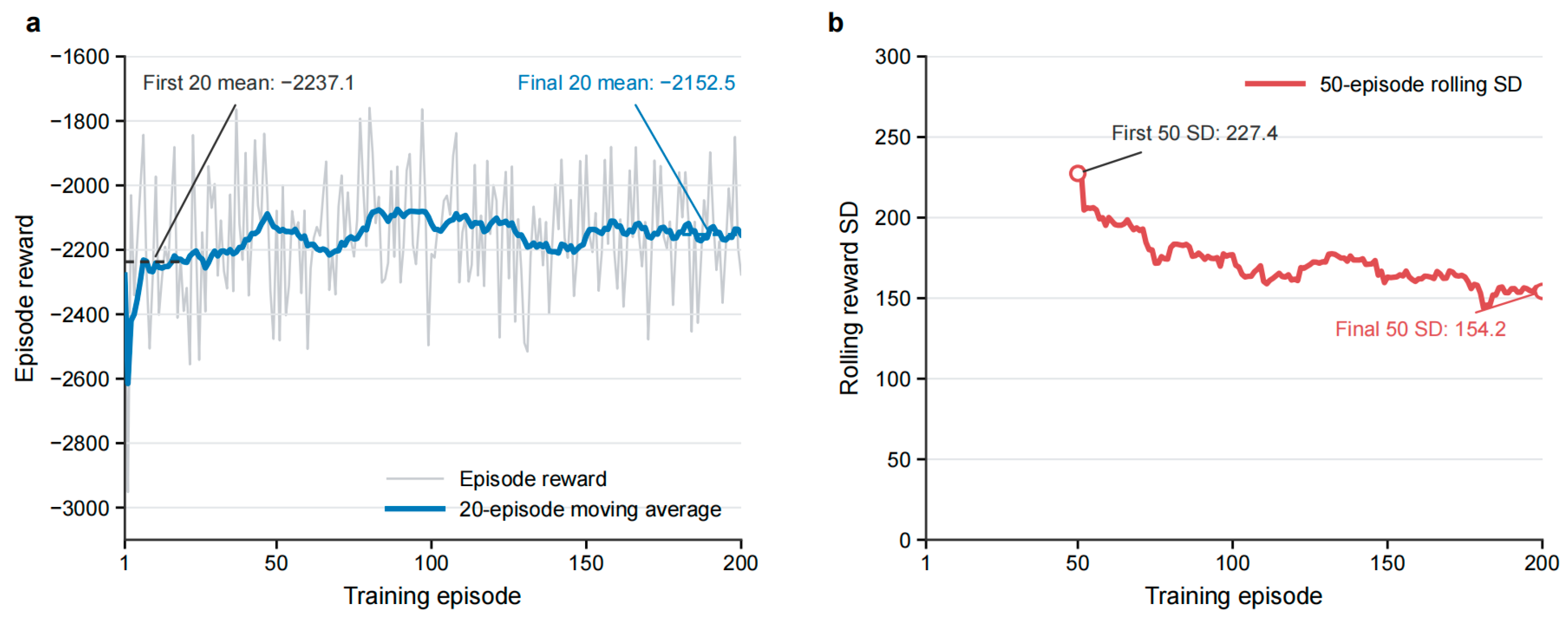
Table A1.
Baseline MPC weights and TD3 action-to-weight mapping parameters.
Appendix B
Based on the state variables, suspension forces, tire forces, and vehicle dynamic equations defined in Equations (1)–(11), the complete matrix representation of the seven-degree-of-freedom full-vehicle model is derived below.
The displacement coordinates contained in the state vector are collected as
The vertical displacements of the four suspension mounting points on the vehicle body satisfy
where,
and
The vertical displacements of the four unsprung masses are expressed as
where
and
The suspension dynamic-deflection vector is therefore
where
The tire-deformation vector is
where the road-input vector is .
The suspension stiffness, suspension damping, tire stiffness, and generalized mass matrices are defined as
and
Here, denotes the vehicle-body sprung mass, denotes the pitch moment of inertia about the lateral axis, denotes the roll moment of inertia about the longitudinal axis, and denotes the unsprung mass at the suspension position, where .
The active suspension control-force vector is
By combining the force and moment equilibrium equations of the sprung and unsprung masses, the full-vehicle dynamics can be written as
where
and
The matrix maps the four active suspension control forces into the generalized vertical force, pitch moment, roll moment, and unsprung-mass forces. The matrix describes the influence of the four-wheel road inputs on the vehicle dynamics.
For the grouped state coordinates, define
The corresponding continuous-time state-space representation is
where
and
The state vector defined in Equation (1) is arranged in an interleaved displacement-velocity form:
Accordingly, the grouped state vector and the original state vector satisfy
where P is the fixed permutation matrix
and denotes the
standard basis vector. Since
is a permutation matrix,
Therefore, the continuous-time system matrices in Equation (12) are
and
This transformation only rearranges the state variables and does not change their physical definitions or introduce additional degrees of freedom.
The performance output vector defined in Equation (14) is
Define the selection matrix
The first three elements of can be obtained from the first three components of . Therefore, in the grouped state coordinates, the output equation is
where
and
The output matrices corresponding to the state ordering in Equation (1) are consequently
The first three rows of the output equation describe the vehicle-body vertical acceleration, pitch angular acceleration, and roll angular acceleration. The next four rows describe the four suspension dynamic deflections, whereas the last four rows describe the four tire deformations.
Using the sampling time , the continuous-time model is discretized by the zero-order-hold method:
and
The resulting discrete-time full-vehicle model is
where
The dimensions of the continuous and discrete system matrices are
and
The above matrix representation is mathematically equivalent to the scalar vehicle dynamic equations in Equations (8)–(11) and constitutes the full-vehicle prediction model used in the MPC optimization.
References
- Liu, Q.; Hu, B.; Liu, W.; Li, J.; Yu, W.; Li, G.; Hu, G. A Fractional-Order Model Predictive Control Strategy with Takagi-Sugeno Fuzzy Optimization for Vehicle Active Suspension System. Fractal Fract. 2024, 8, 610. [Google Scholar] [CrossRef] [Scilit]
- Jiang, Y.; Wang, R.; Ding, R.; Ye, Q. Dual-Loop Model Predictive Control of Permanent Magnet Linear Synchronous Motor for Active Suspension. IEEE Trans. Energy Convers. 2025, 40, 80–92. [Google Scholar] [CrossRef] [Scilit]
- Yang, L.; Wang, G.; Cui, H.; Liu, W.; Zhang, L. Longitudinal, Lateral, and Vertical Coordinated Control of Active Hydro-Pneumatic Suspension System Based on Model Predictive Control for Mining Dump Truck. Machines 2026, 14, 133. [Google Scholar] [CrossRef] [Scilit]
- Liu, Y.; Pang, H.; Zhang, X. Model Predictive Control of Active Suspension Systems Based on Event-Triggered Mechanism. In Proceedings of the 2025 9th CAA International Conference on Vehicular Control and Intelligence (CVCI), Qingdao, China, 24–26 October 2025; pp. 1–6. [Google Scholar] [CrossRef] [Scilit]
- Jung, J.Y.; Lee, C. Preview Model Predictive Control of Semi-active Suspension for Speed Bump. Int. J. Automot. Technol. 2025, 26, 1115–1126. [Google Scholar] [CrossRef] [Scilit]
- Theunissen, J.; Sorniotti, A.; Gruber, P.; Fallah, S.; Ricco, M.; Kvasnica, M.; Dhaens, M. Regionless Explicit Model Predictive Control of Active Suspension Systems with Preview. IEEE Trans. Ind. Electron. 2019, 67, 4877–4888. [Google Scholar] [CrossRef] [Scilit]
- Rodriguez-Guevara, D.; Favela-Contreras, A.; Beltran-Carbajal, F.; Sotelo, C.; Sotelo, D. A Differential Flatness-Based Model Predictive Control Strategy for a Nonlinear Quarter-Car Active Suspension System. Mathematics 2023, 11, 1067. [Google Scholar] [CrossRef] [Scilit]
- Li, S. A Novel L2-Gain Model Predictive Speed Control of Permanent Magnet Synchronous Motors with Recursive Feasibility. J. Electr. Eng. Technol. 2026, 21, 1963–1979. [Google Scholar] [CrossRef] [Scilit]
- Wang, P.; Ren, X.; Zheng, D. Aperiodic Data-Driven Model Predictive Control with Feasibility and Stability Guarantees. IEEE Trans. Autom. Sci. Eng. 2025, 22, 14461–14473. [Google Scholar] [CrossRef] [Scilit]
- Fiacchini, M.; Mammarella, M.; Dabbene, F. Measured-state conditioned recursive feasibility for stochastic model predictive control. Int. J. Robust Nonlinear Control 2026, 36, 5964–5981. [Google Scholar] [CrossRef] [Scilit]
- Landgraf, D.; Völz, A.; Graichen, K. Recursive Feasibility of Nonlinear Stochastic Model Predictive Control with Gaussian Process Dynamics. Int. J. Robust Nonlinear Control 2026, 36, 4957–4970. [Google Scholar] [CrossRef] [Scilit]
- Geurts, M.E.; Katriniok, A.; Silvas, E.; Brouwer, N.J.; Heemels, W.P.M.H. Model Predictive Control for Lane Merging Automation with Recursive Feasibility Guarantees and Its Experimental Validation. IEEE Trans. Control Syst. Technol. 2025, 33, 566–581. [Google Scholar] [CrossRef] [Scilit]
- Wang, G.; Deng, J.; Duan, D.; Zhou, T.; Liu, S. Constrained H∞ Optimal Control for Nonlinear Active Suspensions Via Data-Driven Reinforcement Learning Algorithm. J. Comput. Nonlinear Dyn. 2025, 20, 071007. [Google Scholar] [CrossRef] [Scilit]
- Lee, D.; Jin, S.; Lee, C. Deep Reinforcement Learning of Semi-Active Suspension Controller for Vehicle Ride Comfort. IEEE Trans. Veh. Technol. 2023, 72, 327–339. [Google Scholar] [CrossRef] [Scilit]
- Kozek, M.; Smoter, A.; Lalik, K. Neural-Assisted Synthesis of a Linear Quadratic Controller for Applications in Active Suspension Systems of Wheeled Vehicles. Energies 2023, 16, 1677. [Google Scholar] [CrossRef] [Scilit]
- Han, S.-Y.; Liang, T. Reinforcement-Learning-Based Vibration Control for a Vehicle Semi-Active Suspension System via the PPO Approach. Appl. Sci. 2022, 12, 3078. [Google Scholar] [CrossRef] [Scilit]
- Wang, G.; Kou, F.; Liu, P.; Lv, W.; Xing, L. Road preview method for active suspension based on reinforcement learning. Meas. Sci. Technol. 2025, 36, 036206. [Google Scholar] [CrossRef] [Scilit]
- Sun, Z.; Jin, W.; Wu, F.; Han, Q.; Wu, Y. An Adaptive Weight Model Predictive Control Strategy for Vienna Rectifiers Under Unbalanced Loads. Int. J. Circuit Theory Appl. 2025, 53, 5228–5242. [Google Scholar] [CrossRef] [Scilit]
- Gamal, Z.; Mahran, Y.; El-Badawy, A. Control of a Twin Rotor using Twin Delayed Deep Deterministic Policy Gradient (TD3). In Proceedings of the 2024 28th International Conference on System Theory, Control and Computing (ICSTCC), Sinaia, Romania, 10–12 October 2024; pp. 329–335. [Google Scholar] [CrossRef] [Scilit]
- Demircioğlu, U.; Bakır, H.; Almarri, B.; Abdul Hafez, A.H. TD3-Based Reinforcement Learning for Adaptive PID-like Control of Uncertain Dynamical Systems. Mathematics 2026, 14, 1744. [Google Scholar] [CrossRef] [Scilit]
- Fujimoto, S.; Van Hoof, H.; Meger, D. Addressing Function Approximation Error in Actor-Critic Methods. Proc. Mach. Learn. Res. 2018, PMLR 80, 1587–1596. [Google Scholar] [CrossRef] [Scilit]
- Qiu, J.; Tian, K.; Yan, K. Research on the Tracking and Landing Control of Quadrotor Unmanned Aerial Vehicles Based on Hyperbolic Spiral Sliding Mode Control and TD3 Neural Network. In Proceedings of the 2025 8th International Conference on Robotics, Control and Automation Engineering (RCAE), Xi’an, China, 24–26 October 2025. [Google Scholar] [CrossRef] [Scilit]
- Hu, W.; Wang, Y.; Chen, Q.; Wang, P.; Wu, E.; Guo, Z.; Hou, Z. TD3 Agent-Based Nonlinear Dynamic Inverse Control for Fixed-Wing UAV Attitudes. IEEE Trans. Intell. Transp. Syst. 2025, 27, 2607–2618. [Google Scholar] [CrossRef] [Scilit]
- Dong, S.; Yang, H.; Xie, C.-H.; Zhou, Y. Multiple High-Speed Trains Cooperative Tracking Control Based on Distributed Adaptive Model Predictive Control. IEEE Trans. Autom. Sci. Eng. 2026, 23, 2864–2877. [Google Scholar] [CrossRef] [Scilit]
- Nguyen, T.T.; Tran, H.N.; Nguyen, T.H.; Jeon, J.W. Recurrent Neural Network-Based Robust Adaptive Model Predictive Speed Control for PMSM with Parameter Mismatch. IEEE Trans. Ind. Electron. 2023, 70, 6219–6228. [Google Scholar] [CrossRef] [Scilit]
- Wang, C.; Cui, X.; Zhao, S.; Zhou, X.; Song, Y.; Wang, Y.; Guo, K. A deep reinforcement learning-based active suspension control algorithm considering deterministic experience tracing for autonomous vehicle. Appl. Soft Comput. 2024, 153, 15. [Google Scholar] [CrossRef] [Scilit]
- Deng, M.; Sun, D.; Zhan, L.; Xu, X.; Zou, J. Advancing Active Suspension Control with TD3-PSC: Integrating Physical Safety Constraints Into Deep Reinforcement Learning. IEEE Access 2024, 12, 115628–115641. [Google Scholar] [CrossRef] [Scilit]
- Li, Y.; Han, Y.; Chen, C.; Zeng, Z.; Sun, J. Online Reinforcement Learning Control Designs with Acceleration Mechanism for Unknown Multiagent Systems Through Value Iteration. IEEE Trans. Neural Netw. Learn. Syst. 2025, 36, 16990–17003. [Google Scholar] [CrossRef] [Scilit] [PubMed]
- Yan, S.; Sun, W.; Xia, Y. A Joint Fault-Tolerant and Fault Diagnosis Strategy for Multiple Actuator Faults of Full-Vehicle Active Suspension Systems. IEEE Trans. Autom. Sci. Eng. 2025, 22, 1928–1940. [Google Scholar] [CrossRef] [Scilit]
- Emami, A.; Masih-Tehrani, M.; Amirkhani, A.; Najafi, A. Robust Fuzzy Sliding Mode Controller for the Full Vehicle Semi-Active Suspension System Considering the Impact of Uncertainties. IET Intell. Transp. Syst. 2025, 19, e70125. [Google Scholar] [CrossRef] [Scilit]
- Wang, W.; Liu, S.; Zhao, D. A low-complexity fixed-time prescribed performance control for uncertain full-vehicle active suspensions with hydraulic actuators. Int. J. Control 2025, 98, 1272–1283. [Google Scholar] [CrossRef] [Scilit]
- Kim, Y.; Kwak, T.; Kanno, M.; Kim, T.-H. Multi-Objective Finite-Frequency H∞/GH2 Static Output-Feedback Control Synthesis for Full-Vehicle Active Suspension Systems: A Metaheuristic Optimization Approach. IEEE Access 2023, 11, 36309–36330. [Google Scholar] [CrossRef] [Scilit]
- Zhao, R.; Huang, W.; Xie, H. Neural Network-Interacted Robust Coordinated Control of Full-Vehicle Active Air Suspension with Uncertainties and Time Delays. IEEE Access 2024, 12, 141291–141305. [Google Scholar] [CrossRef] [Scilit]
- Tsai, Y.K.; Chen, Y.P.; Karkaria, V.; Chen, W. Reinforcement learning-based control co-design of digital twin-enabled full-vehicle active suspension systems. Struct. Multidiscip. Optim. 2026, 69, 108. [Google Scholar] [CrossRef] [Scilit] [PubMed]
- ISO 8608:2016; Mechanical Vibration—Road Surface Profiles—Reporting of Measured Data. International Organization for Standardization: Geneva, Switzerland, 2016.
- Jagadeshwar, M.; Das, D.K. A Novel Adaptive Model Predictive Control Scheme with Incremental Conductance for Extracting Maximum Power from a Solar Panel. Iran. J. Sci. Technol. Trans. Electr. Eng. 2022, 46, 653–664. [Google Scholar] [CrossRef] [Scilit]
- Oh, S.C.; Song, T.J.; Kim, M.J.; Oh, K.S. Adaptive Model Predictive Fault-Tolerant Control for Four-Wheel Independent Steering Vehicles with Sensitivity Estimation. Int. J. Automot. Technol. 2023, 24, 829–850. [Google Scholar] [CrossRef] [Scilit]
- Zhang, X.; Yu, X.; Zhang, G. Adaptive Model Predictive Current Control for PMSM Drives Based on Bayesian Inference. IEEE Trans. Power Electron. 2025, 40, 8490–8502. [Google Scholar] [CrossRef] [Scilit]
- Putri, S.A.; Shadaei, M.; Moazeni, F.; Khazaei, J. Stability and Feasibility-Driven Predictive Control for Next-Generation Naval Microgrids. IEEE Trans. Transp. Electrif. 2025, 11, 3848–3860. [Google Scholar] [CrossRef] [Scilit]
- Osman, O.; Karaca, T.K.; Kavus, B.Y.; Tulum, G. AdvB-TD3: A Novel Decision-Making Framework for Complex Continuous Control Tasks. IEEE Access 2025, 13, 181675–181685. [Google Scholar] [CrossRef] [Scilit]
- Xi, H.; Xie, S.; Yang, Y. Continuous Drifting Control Based on Maximal Safety Probability Learning with TD3 and Lagrangian. In Proceedings of the 2025 IEEE 28th International Conference on Intelligent Transportation Systems (ITSC), Gold Coast, Australia, 18–21 November 2025. [Google Scholar] [CrossRef] [Scilit]
- Zarrouki, B.; Spanakakis, M.; Betz, J. A Safe Reinforcement Learning driven Weights-varying Model Predictive Control for Autonomous Vehicle Motion Control. In 2024 IEEE Intelligent Vehicles Symposium (IV); IEEE: New York, NY, USA, 2024. [Google Scholar] [CrossRef] [Scilit]
- Pfrommer, S.; Gautam, T.; Zhou, A.; Sojoudi, S. Safe Reinforcement Learning with Chance-constrained Model Predictive Control. arXiv 2021. [Google Scholar] [CrossRef] [Scilit]
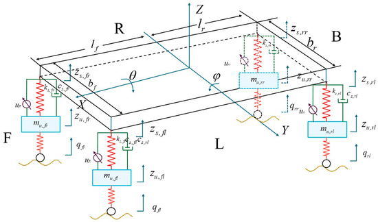
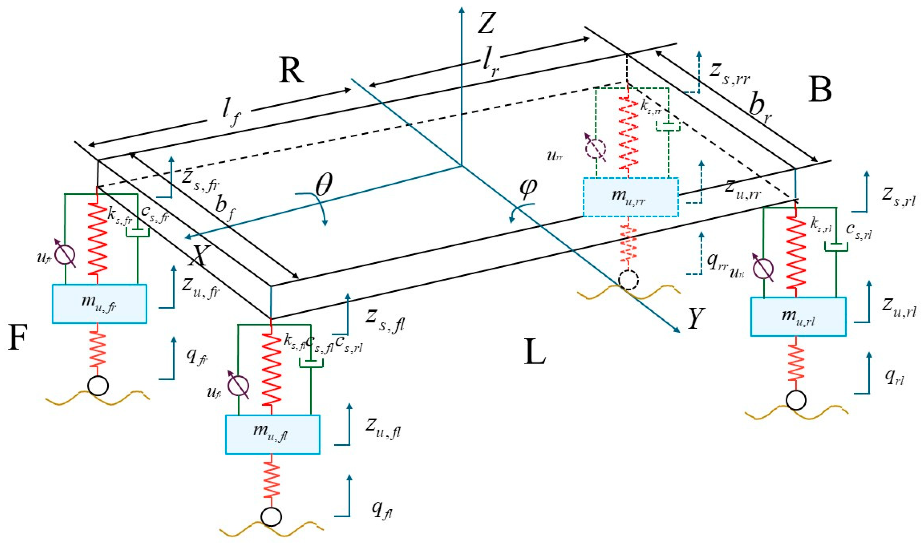
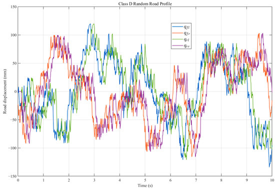
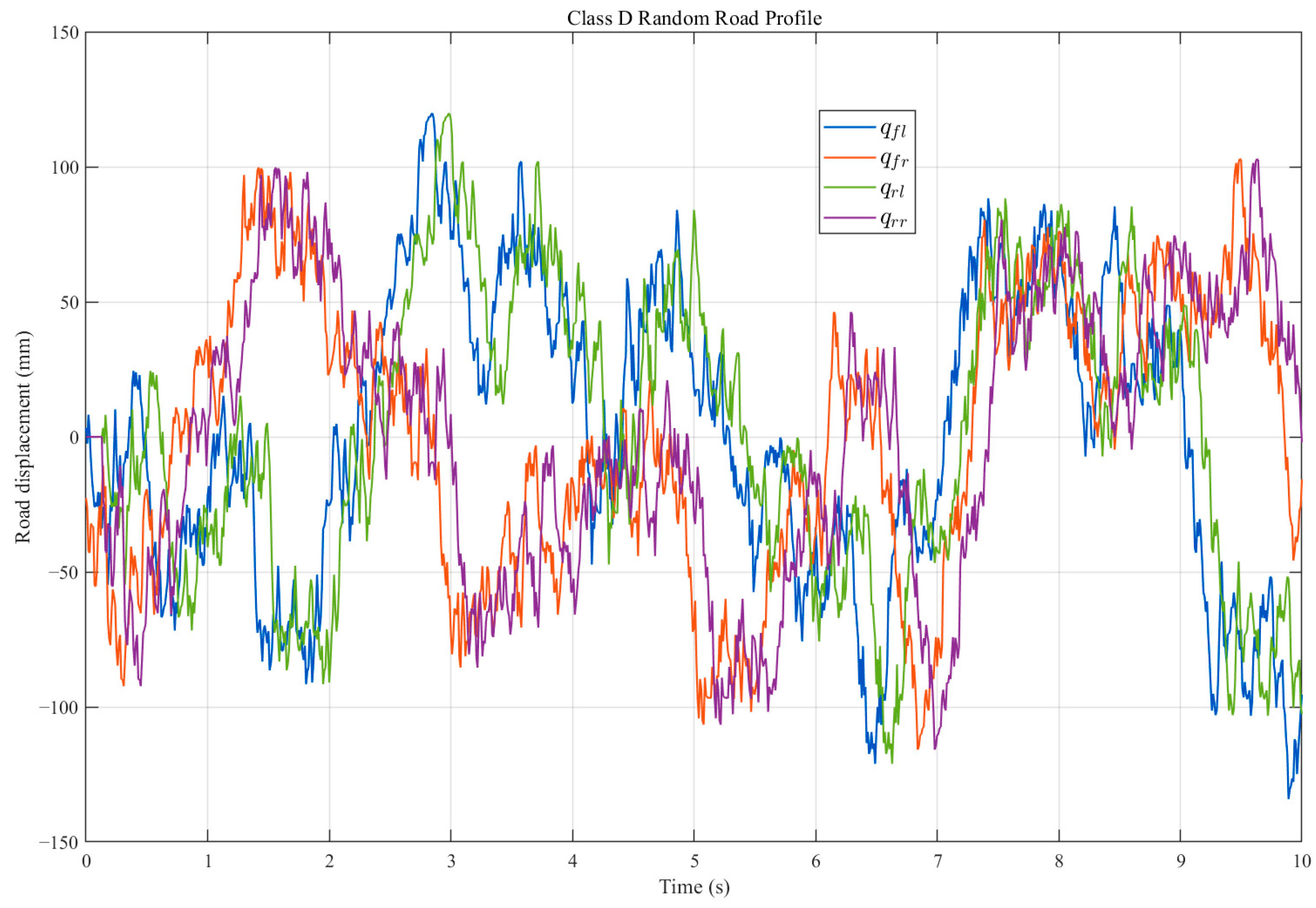
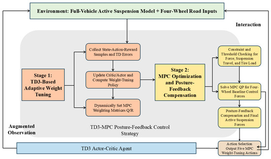
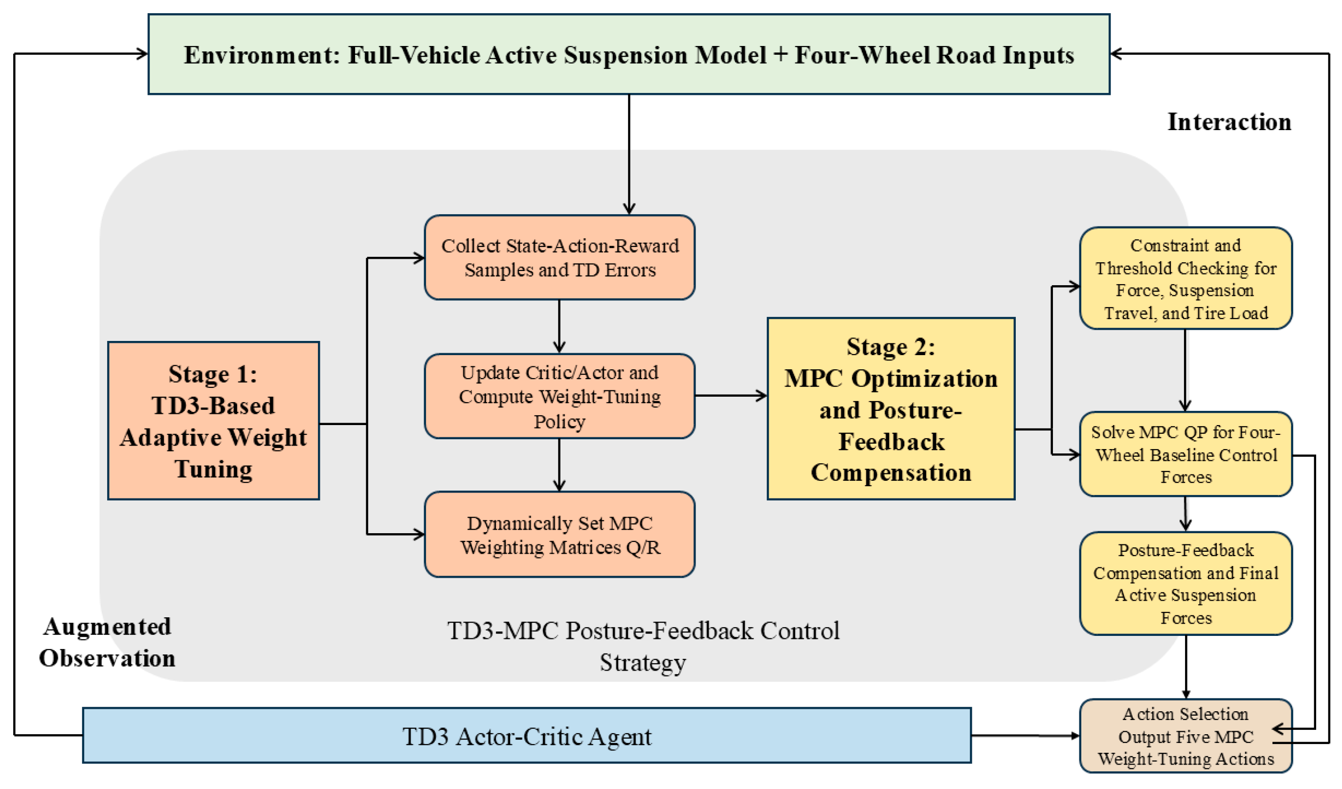
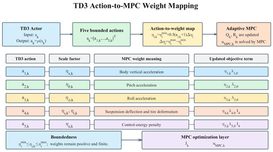
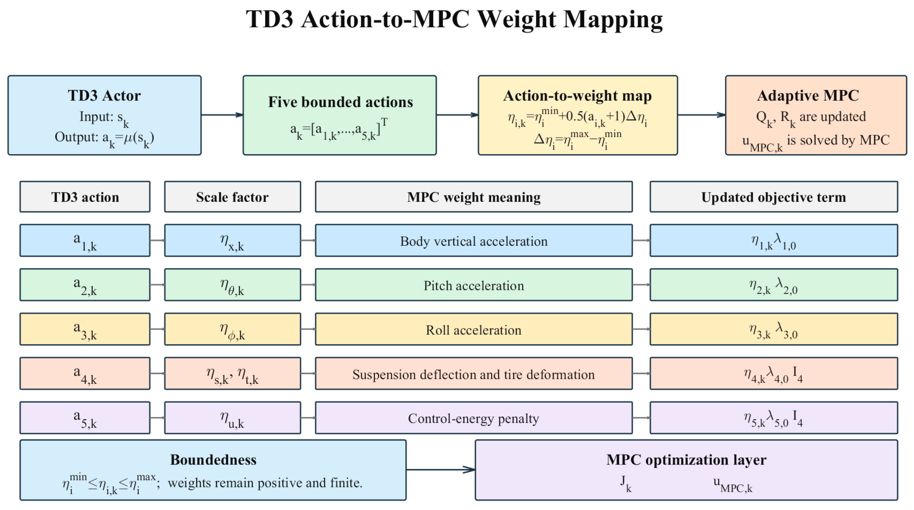
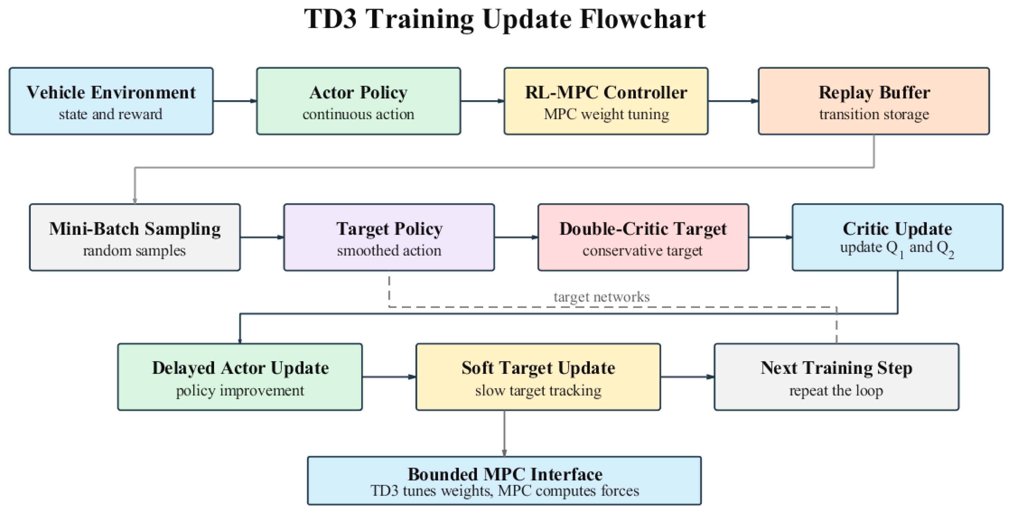
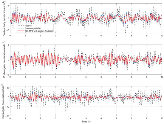
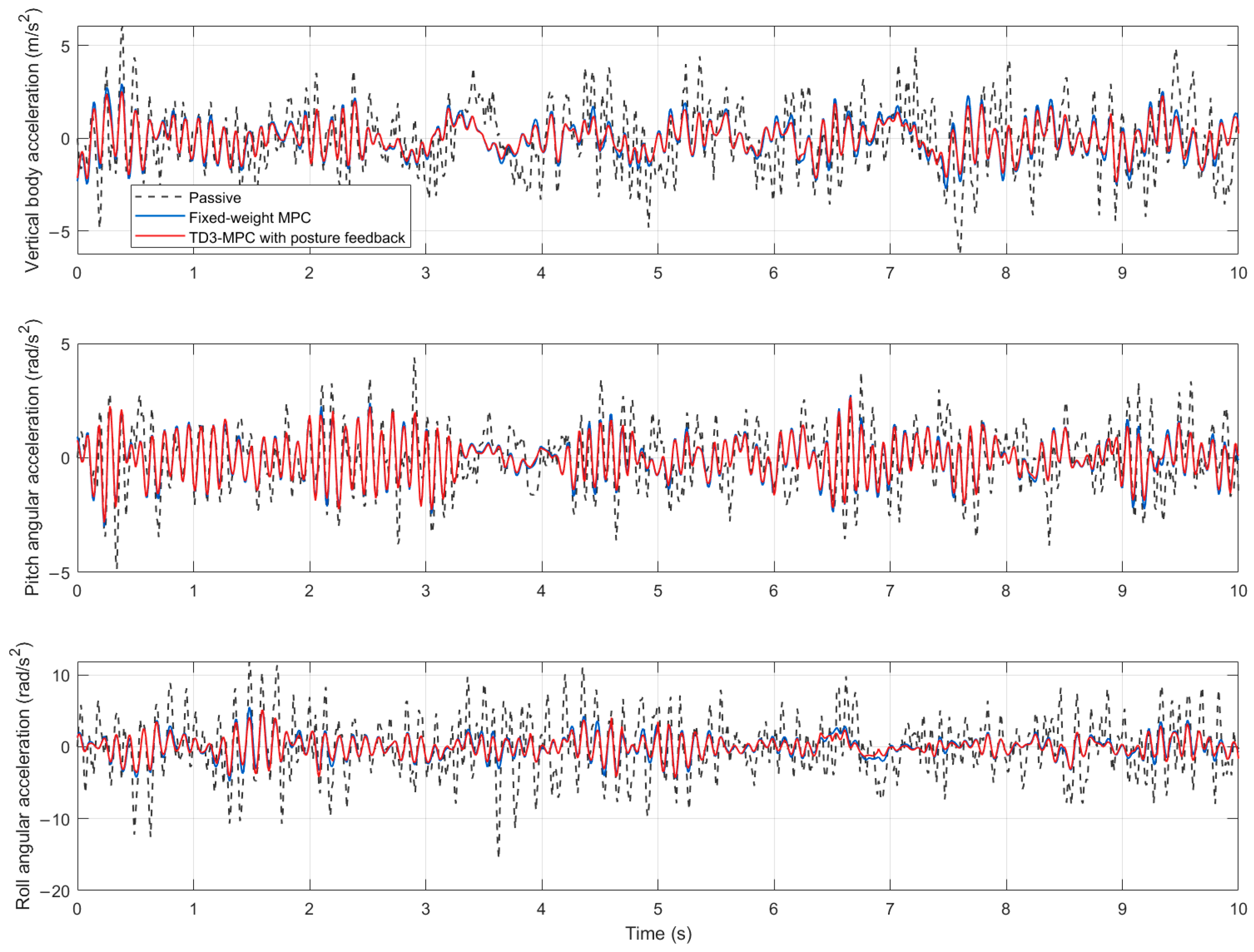
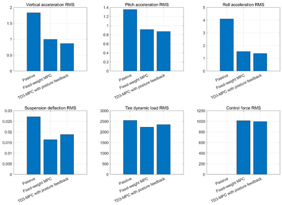
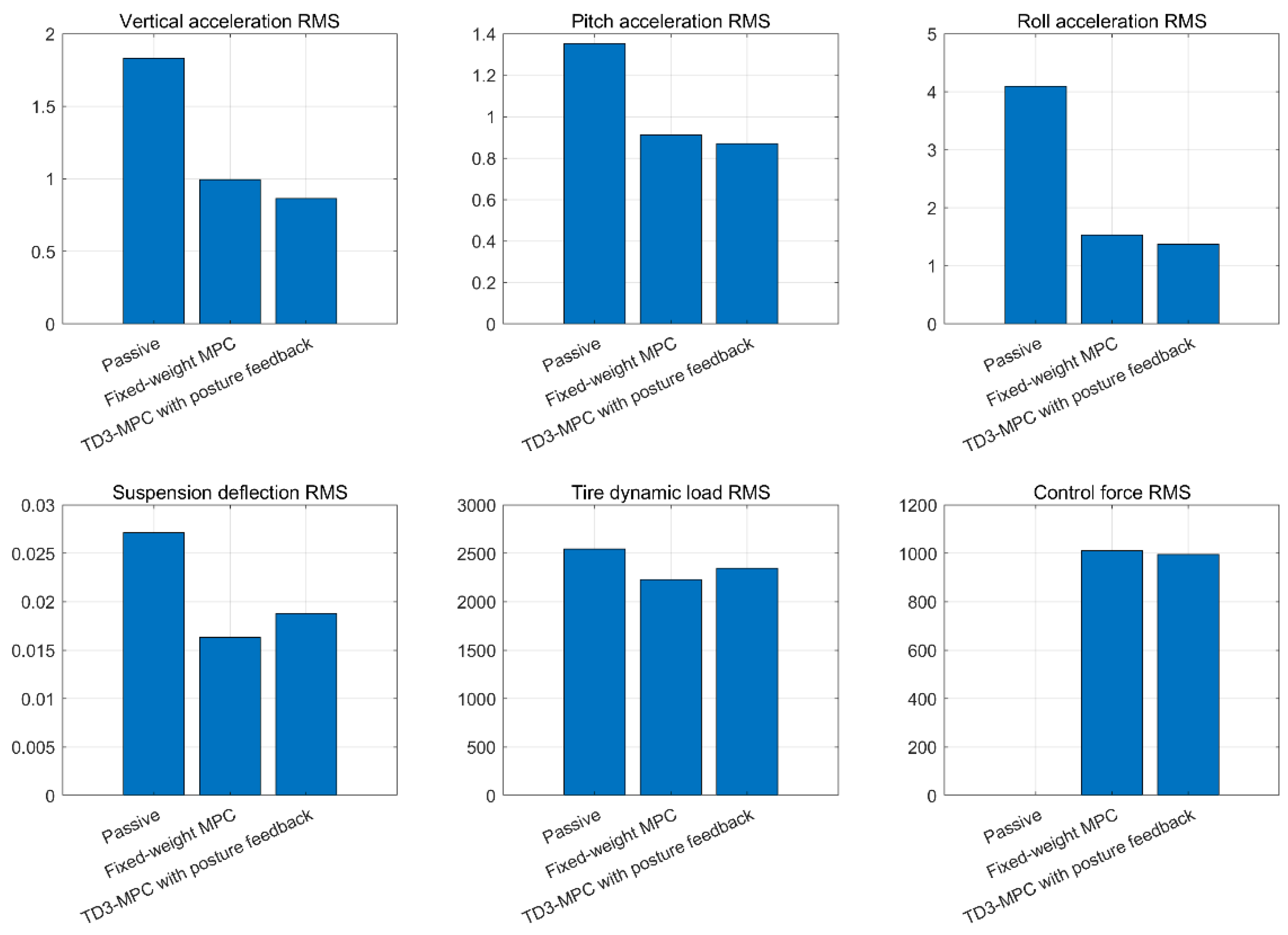
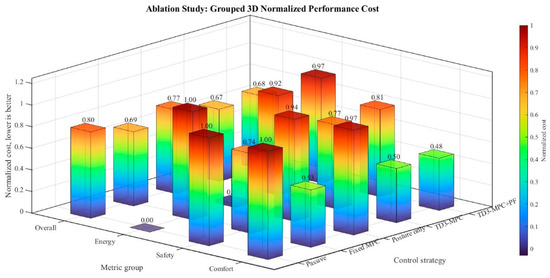
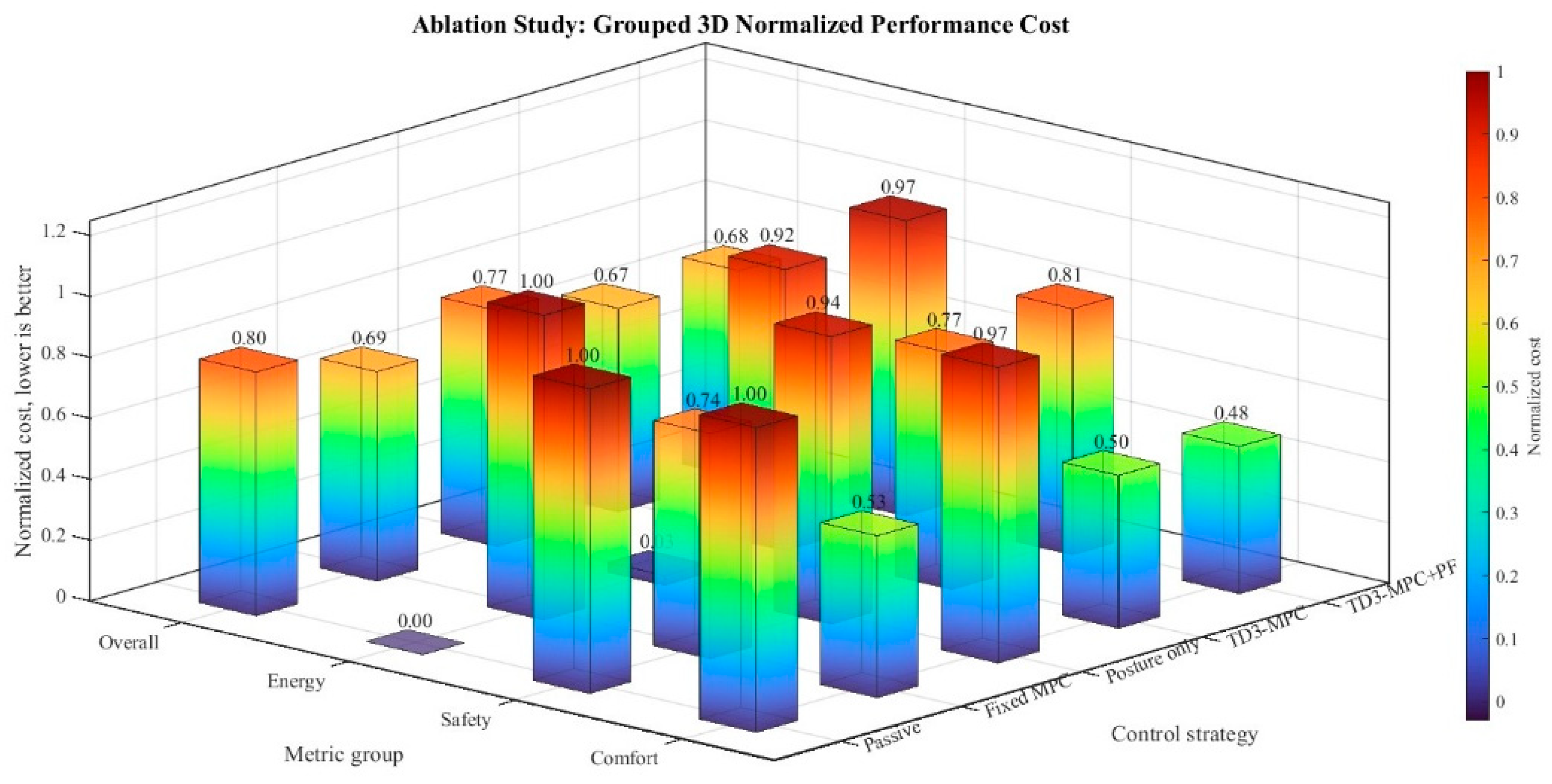
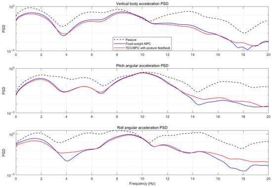
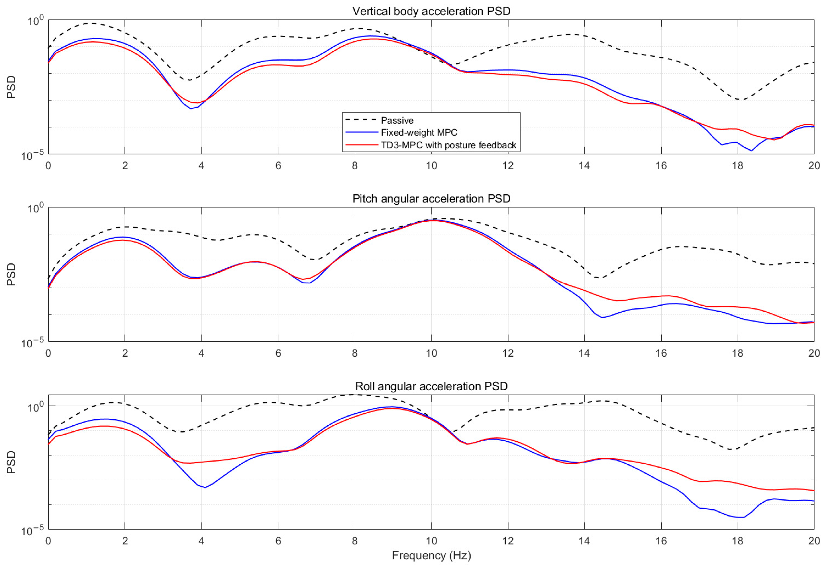
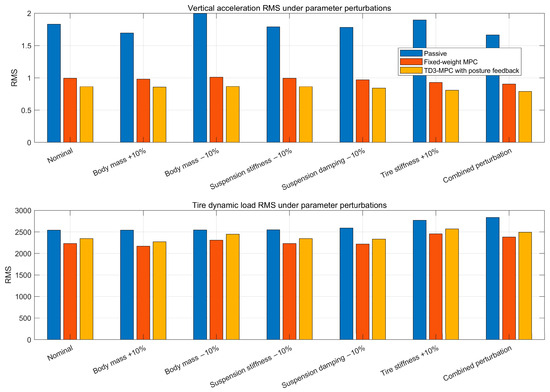
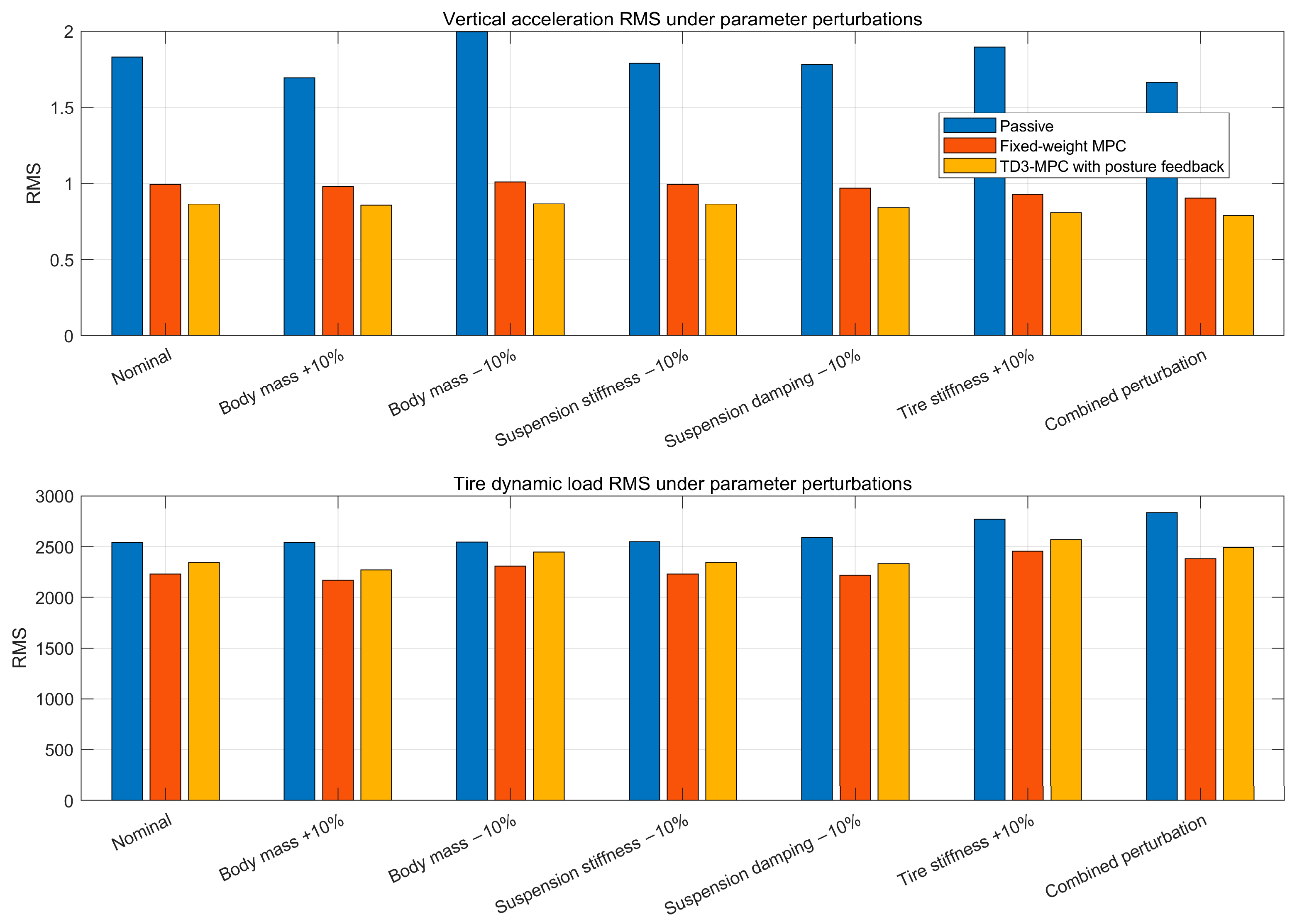
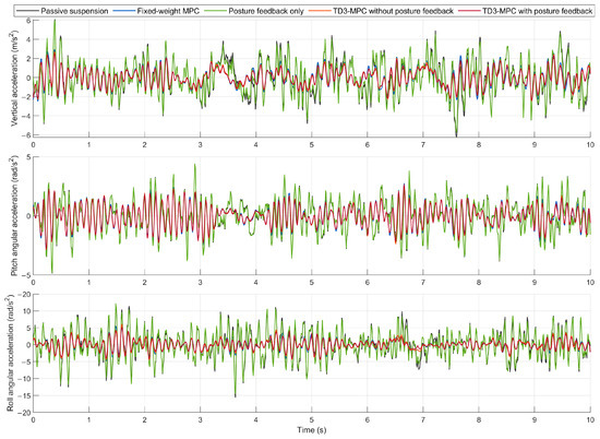
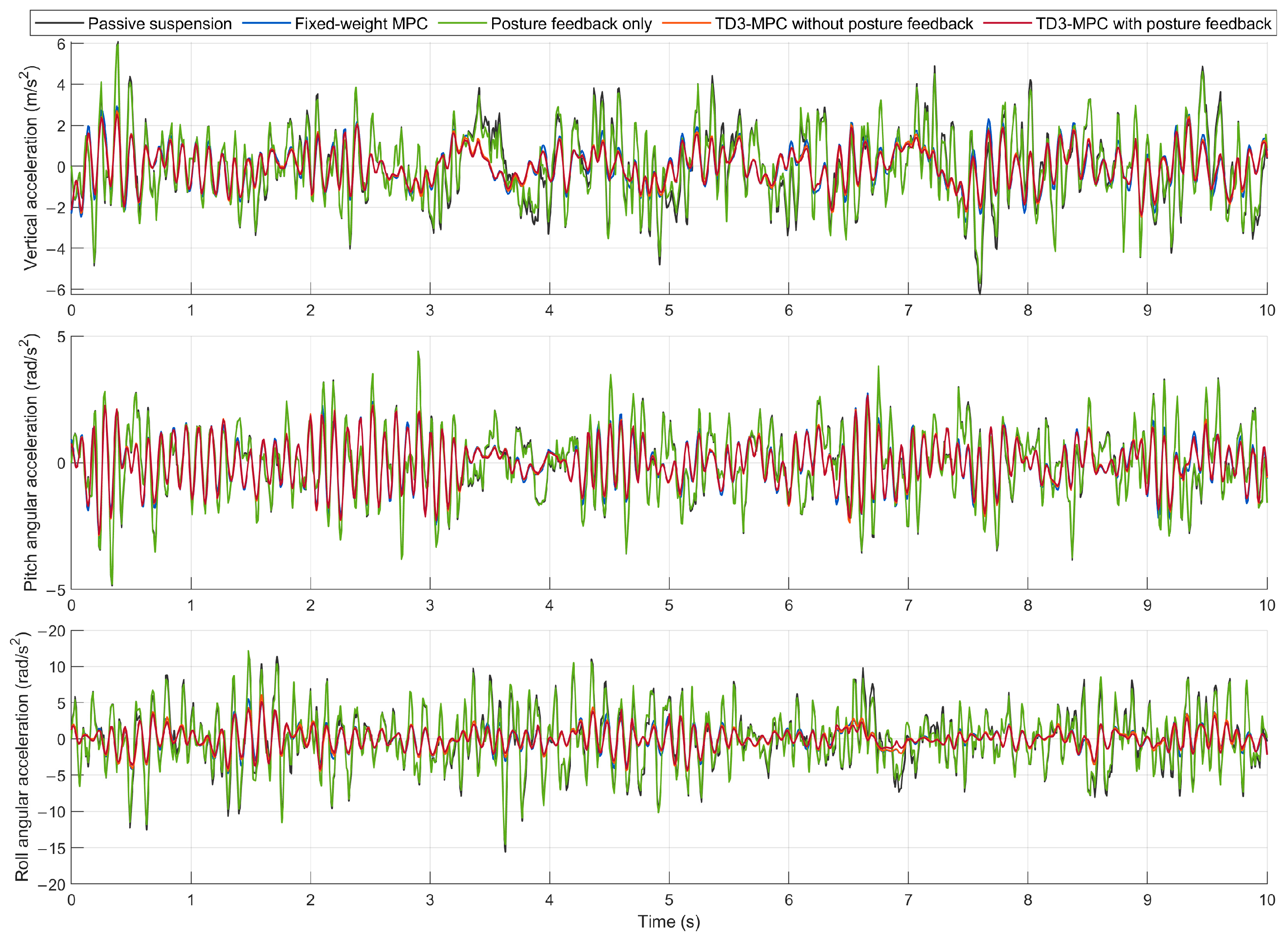
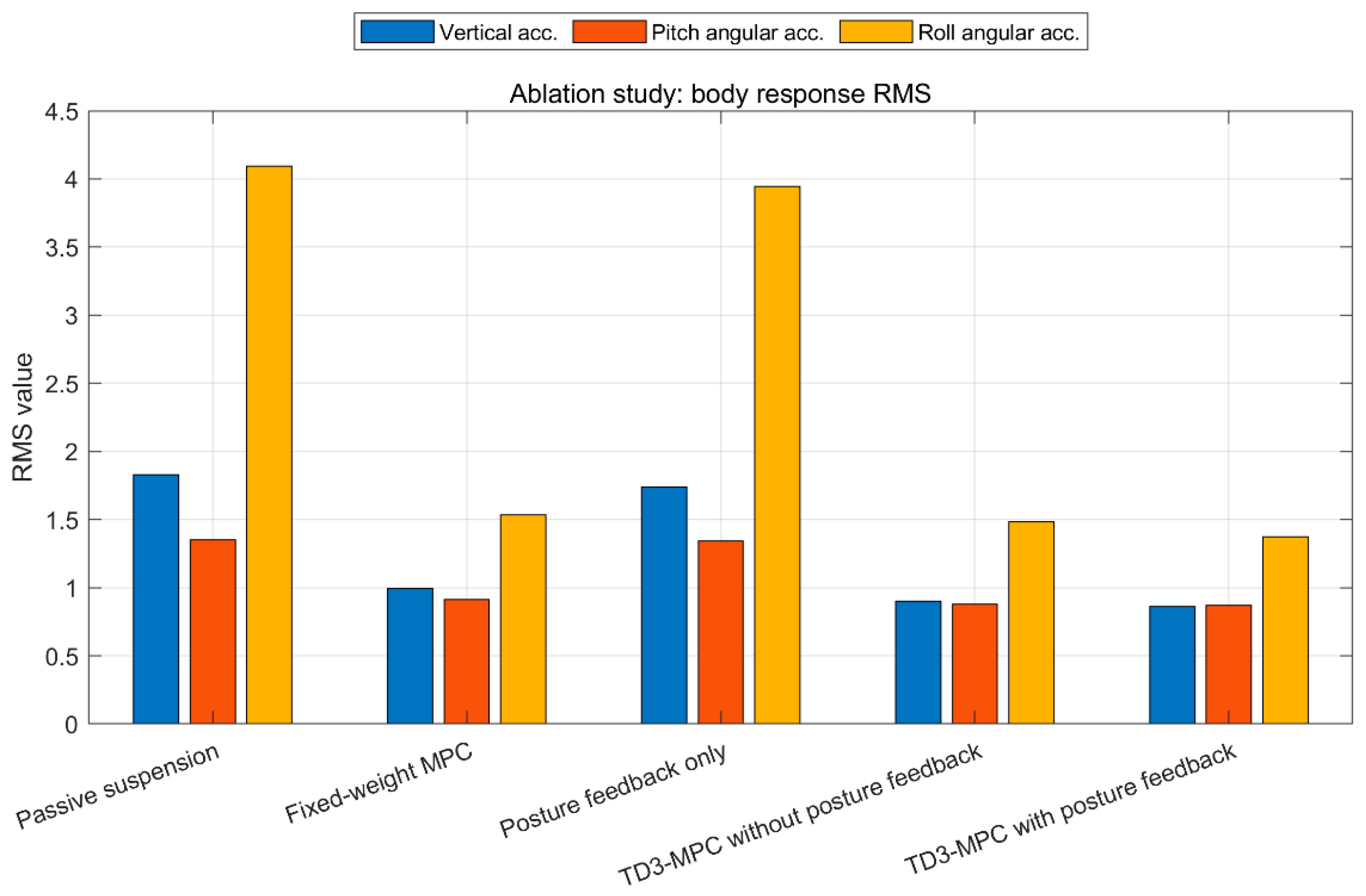
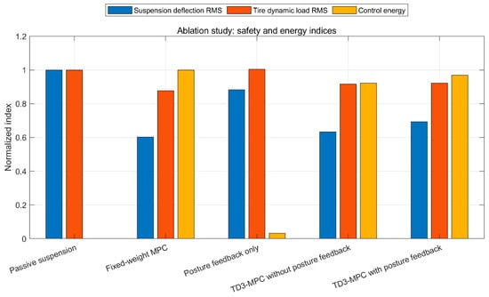
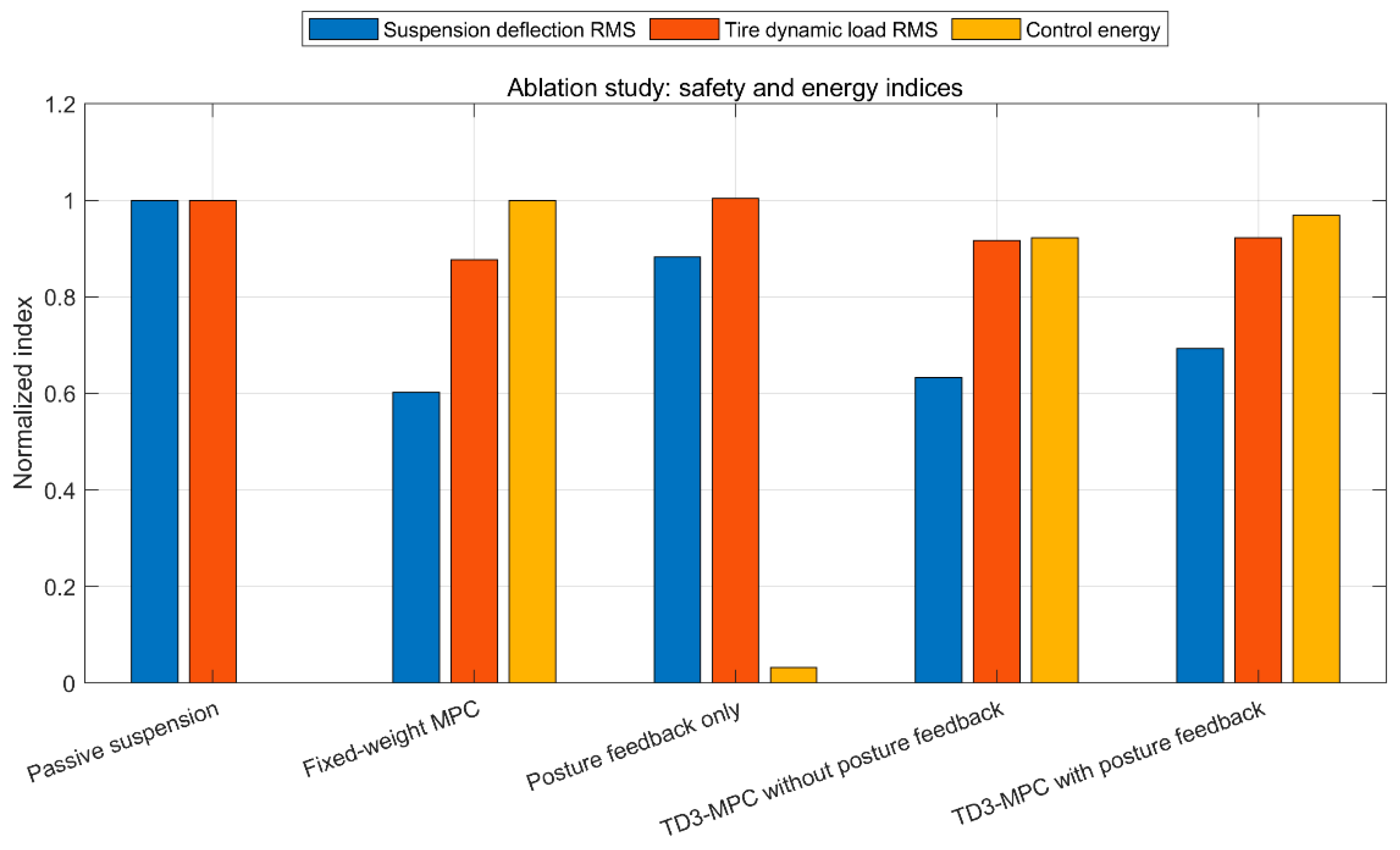
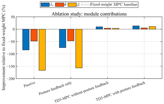
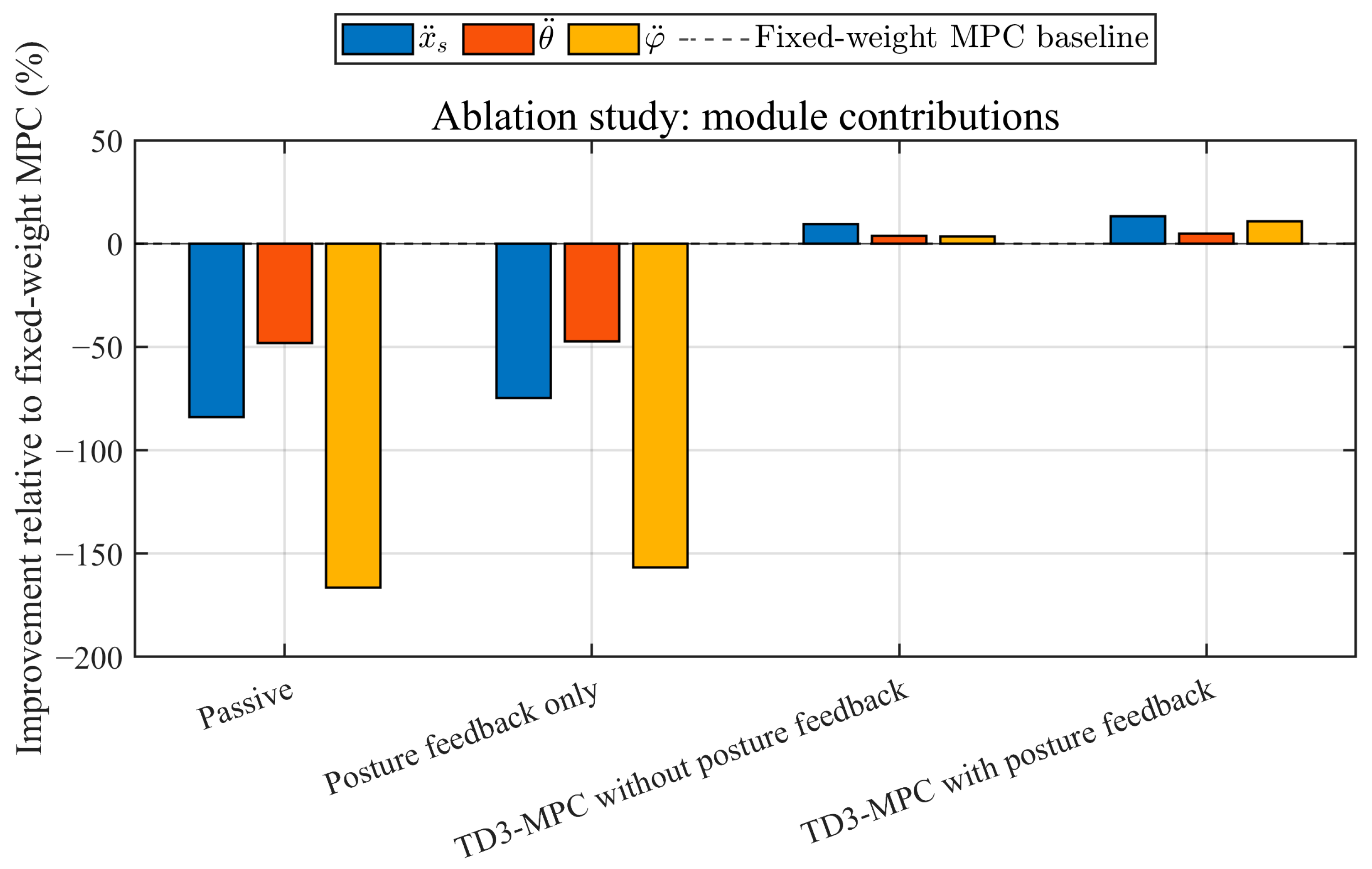
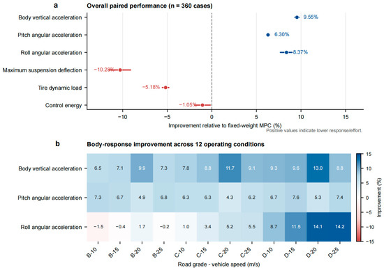
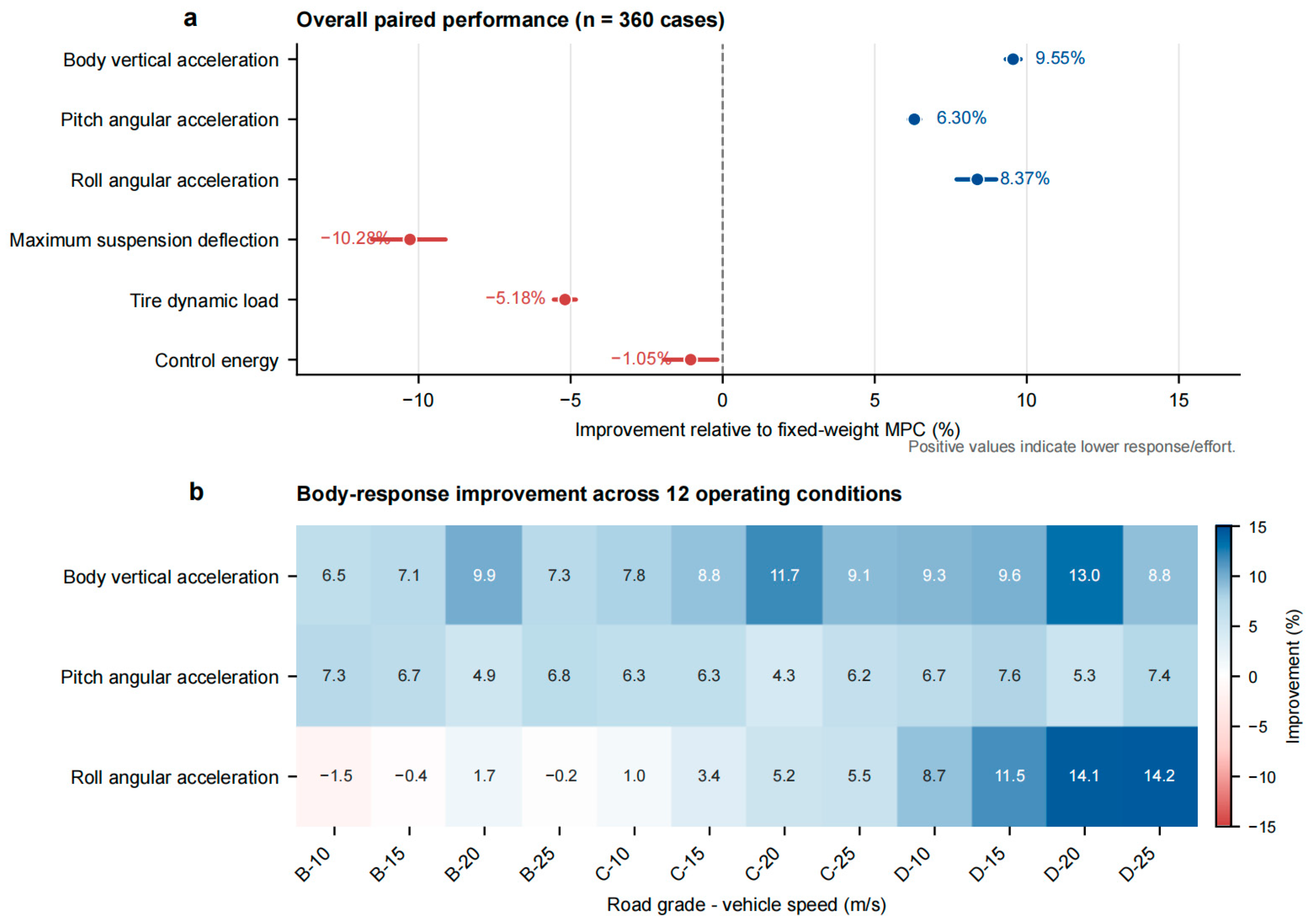

Disclaimer/Publisher’s Note: The statements, opinions and data contained in all publications are solely those of the individual author(s) and contributor(s) and not of MDPI and/or the editor(s). MDPI and/or the editor(s) disclaim responsibility for any injury to people or property resulting from any ideas, methods, instructions or products referred to in the content. |
© 2026 by the authors. Licensee MDPI, Basel, Switzerland. This article is an open access article distributed under the terms and conditions of the Creative Commons Attribution (CC BY) license.