


Abstract
Portfolio optimization models are highly sensitive to estimation errors in expected returns and covariance matrices, often resulting in unstable allocations. Robust optimization mitigates parameter uncertainty by optimizing against worst-case realizations within a specified uncertainty set, whose construction critically determines the effectiveness of the approach. This paper proposes a data-driven framework for constructing polyhedral uncertainty sets that integrates Gaussian mixture models (GMMs) to identify heterogeneous distributional components and ARIMA-GARCH models to capture time-varying volatility dynamics. The construction proceeds in three stages. First, ARIMA-GARCH filters remove serial dependence and volatility clustering. Second, GMM clustering applied to the standardized residuals identifies latent market regimes. Third, convex hulls of observations lying within a Mahalanobis distance threshold form component-wise polyhedral sets, which are aggregated into a global convex uncertainty set. The robust counterpart is derived via linear programming duality, transforming the robust constraint into a tractable quadratic program that preserves convexity and polyhedrality. We prove that the constructed sets are convex and polyhedral, establish probabilistic coverage guarantees under mild regularity conditions, and analyze the computational complexity of the framework. Empirical analysis of Indonesian equity data confirms heavy tails and volatility clustering, with GMM identifying three distinct regimes of approximately equal proportions. Controlled synthetic experiments show that uncertainty set geometry fundamentally influences portfolio outcomes: overlapping clusters yield stable allocations across regimes, whereas well-separated clusters reveal that convex hull aggregation introduces conservatism that masks regime distinctions. Rolling window backtests demonstrate that the proposed approach produces economically higher Sharpe ratios than standard uncertainty set formulations in the reported out-of-sample period, although statistical significance is limited by the small number of independent rebalancing periods (18 quarterly events). The practical advantage should therefore be interpreted as conditional on moderate transaction costs and manageable turnover. These findings provide a statistically grounded, geometrically faithful, and computationally tractable methodology for practical implementation, contributing to financial resilience and sustainable economic growth with broader implications for stable capital markets.
Keywords:
robust optimization; portfolio optimization; uncertainty set; ARIMA–GARCH; Gaussian mixture model; convex hull MSC:
91G10; 90C17; 62H30; 62M10; 62P05; 90C20; 90C90
1. Introduction
Portfolio optimization is a fundamental problem in quantitative finance, aiming to allocate capital across assets to balance risk and return. The classical mean-variance framework introduced by Markowitz [1] formulates portfolio selection as a quadratic programming problem in which investors minimize portfolio variance subject to expected return and budget constraints. Since its introduction, the mean-variance model has become the cornerstone of modern portfolio theory and continues to play a central role in both academic research and practical asset allocation [2,3].
Despite its theoretical elegance, the performance of the mean-variance model depends critically on the estimation of its input parameters, namely expected returns and the covariance matrix of asset returns. Portfolio optimization is highly sensitive to estimation errors in these parameters. Even small perturbations in estimated returns may lead to large changes in optimal allocations, often resulting in unstable and poorly diversified portfolios [4,5]. This sensitivity is compounded by the statistical properties of financial return data, which frequently exhibit heavy-tailed distributions, volatility clustering, and heterogeneous patterns that deviate substantially from classical assumptions [6,7,8]. Regime-based tactical asset allocation has been shown to improve portfolio performance across business cycles [9].
Robust optimization provides a systematic framework for addressing parameter uncertainty. In this approach, uncertain parameters belong to a predefined uncertainty set, and the problem is solved against the worst-case realization within that set [10,11]. By transforming the uncertain problem into a deterministic robust counterpart, robust optimization ensures feasibility for all realizations within the uncertainty region. Robust optimization has been widely applied to portfolio selection and has demonstrated improved stability compared with classical mean-variance models [12,13,14].
Nevertheless, the effectiveness of robust portfolio optimization depends critically on how the uncertainty set is constructed. Classical uncertainty sets are often specified a priori using simple geometric structures such as box or ellipsoidal sets [10,15]. Although these sets lead to tractable formulations, they may fail to capture complex empirical characteristics of financial return distributions, including heavy tails, asymmetries, and nonlinear dependencies. Uncertainty in portfolio optimization has also been addressed through robustness-based approaches under epistemic uncertainty [16]. Distributionally robust optimization has been extended to incorporate side information [17] and end-to-end portfolio construction [18]. To address this limitation, recent research has explored distributionally robust optimization, where uncertainty is modeled at the distribution level rather than individual parameter values [19,20,21]. Machine learning techniques have also been used to construct uncertainty sets directly from empirical data, using clustering methods and density estimation to identify heterogeneous distributional components [22,23,24,25,26].
In contrast to these existing approaches, the proposed framework offers four distinct advantages that are systematically integrated into a unified methodology:
- 1.
- Data-driven shape: The uncertainty set is constructed from the convex hull of empirical observations. This allows the set to adapt to the actual distributional shape of the data, capturing heavy tails and asymmetries.
- 2.
- Volatility scaling: ARIMA-GARCH filtering incorporates time-varying volatility, ensuring that the uncertainty set scales dynamically with market conditions. This addresses the volatility clustering phenomenon that is pervasive in financial returns.
- 3.
- Regime awareness: GMM clustering captures distributional heterogeneity by identifying distinct market regimes (e.g., neutral, bullish, high-volatility). The resulting regime-specific uncertainty regions reflect the multi-modal nature of financial returns, enabling more nuanced portfolio decisions.
- 4.
- Probabilistic coverage guarantees: The construction provides provable coverage guarantees at the nominal confidence level under mild regularity conditions (see Proposition 2 and Section 5.4). Conventional box and ellipsoidal sets typically lack such guarantees in non-normal, heteroskedastic settings.
Despite these advances, several mathematical challenges remain open in the construction of data-driven polyhedral uncertainty sets for portfolio optimization. First, the integration of time-varying volatility filtering with regime-based clustering. Second, the geometric properties of uncertainty sets constructed from clustered residual observations, specifically convexity and polyhedrality. Third, probabilistic coverage guarantees for such sets have been asserted but not formally proven. Fourth, the computational complexity of constructing polyhedral sets in high-dimensional asset spaces.
This paper addresses these challenges by proposing a data-driven framework for constructing polyhedral uncertainty sets that integrates ARIMA-GARCH filtering for volatility dynamics and Gaussian mixture models (GMMs) for distributional heterogeneity. While convexity of a finite convex hull is a standard result in convex analysis [2,27], its application within a data-driven ARIMA-GARCH-GMM framework to construct component-wise polyhedral uncertainty sets for robust portfolio optimization, along with the formal derivation of probabilistic coverage guarantees and computational complexity analysis, constitutes the main contribution of this work.
Specifically, the proposed framework makes the following contributions. First, the robust portfolio optimization problem is formulated with uncertainty sets constructed from GMM-clustered ARIMA-GARCH residuals. It is established that the resulting component-wise uncertainty sets are convex and polyhedral, and that the global set, defined as the convex hull of their union, preserves these properties (Theorems 2 and 3). The contributions are explicitly distinguished as follows:
- Standard facts (Theorems 2 and 3): convexity and polyhedrality of convex hulls, which follow directly from standard convex analysis [2,27];
- New analytical results (Section 5.3, Section 5.4 and Section 5.5 and Section 6.7): the separation ratio diagnostic for quantifying regime overlap, the characterization of the conservative bias induced by convex hull aggregation, and the empirical validation of coverage guarantees.
Second, probabilistic coverage guarantees are provided for the constructed uncertainty sets, showing that under mild regularity conditions, the global convex hull inherits conservative coverage at the nominal confidence level (Proposition 2). Third, the robust counterpart is derived via linear programming duality, transforming the robust constraint into a tractable quadratic program with linear constraints (Theorem 1). Fourth, the computational complexity of the framework is analyzed, demonstrating that it scales to portfolios of several dozen assets (Proposition 4). Fifth, the practical performance of the proposed framework is illustrated using Indonesian equity data and controlled synthetic experiments, showing that the proposed method achieves superior out-of-sample Sharpe ratios compared to standard uncertainty sets.
The remainder of this paper is organized as follows. Section 2 reviews related literature on robust portfolio optimization and uncertainty set construction. Section 3 formulates the portfolio problem, introduces the necessary preliminaries from convex analysis, and states the assumptions underlying the approach. Section 4 presents the construction of polyhedral uncertainty sets and derives the robust counterpart. Section 5 establishes the theoretical properties of the constructed sets, including convexity, polyhedrality, coverage guarantees, and computational complexity. Section 6 provides numerical illustrations using Indonesian equity data and synthetic experiments. Section 7 concludes the paper.
2. Literature Review
This section reviews the key mathematical developments in robust portfolio optimization, focusing on uncertainty set construction, time-varying volatility modeling, and regime detection. The review identifies persistent mathematical gaps that motivate the proposed framework.
Robust optimization (RO) has emerged as a powerful framework for decision-making under parameter uncertainty [10,11]. In portfolio selection, RO improves stability compared to classical mean-variance models by optimizing against worst-case realizations within a predefined uncertainty set [12,13]. From a mathematical perspective, the core challenge lies in constructing uncertainty sets that are both statistically meaningful and computationally tractable, while capturing the empirical structure of financial returns.
The choice of uncertainty set critically determines both tractability and conservatism. Table 1 provides an objective summary of selected studies, detailing uncertainty set methodology, temporal structure, and validation approach.
Classical uncertainty sets (box, ellipsoid) are often specified a priori and may fail to capture heavy tails, asymmetries, or volatility clustering [10,15]. Shukla et al. [28] compared mixed, box, and ellipsoidal sets, finding that box uncertainty yields the least risk, making it most suitable for risk-averse investors. Yin et al. [29] recommended the quadratic (ellipsoidal) set with a diagonal estimation-error matrix, arguing that box uncertainty is overly conservative. From a mathematical standpoint, these sets yield tractable robust counterparts but lack the flexibility to capture multi-modal and heavy-tailed empirical return distributions.
Data-driven ambiguity sets, such as Wasserstein balls, offer statistical guarantees by constructing uncertainty regions directly from historical observations [20]. Du et al. [20] demonstrated that Wasserstein-based DRO outperforms ambiguity-free stochastic optimization on both Chinese and US markets. Data-driven robust optimization approaches have been further extended to multi-item newsboy problems [30]. Adjustable robust optimization has also been applied to internet shopping problems using Benders decomposition [31]. Sehgal and Jagadesh [22] used support vector clustering to construct convex uncertainty sets, yielding robust portfolios that consistently outperform nominal counterparts. However, these approaches typically rely on historical moments alone and do not incorporate forward-looking volatility forecasts.
Polyhedral uncertainty sets, derived from convex hulls of empirical data, provide a flexible alternative that captures complex distributional shapes while preserving linear constraints [32,33]. Fernandes et al. [32] proposed a data-driven polyhedral set with loss constraints, adaptively updated in a rolling horizon scheme, demonstrating enhanced out-of-sample performance with transaction costs. Adaptive robust online portfolio selection has also been explored to handle dynamic market environments [34]. Closed-form optimal portfolios have been derived for distributionally robust mean-CVaR problems [35]. Despite these advances, a rigorous mathematical framework that explicitly integrates time-varying volatility and regime-dependent heterogeneity into polyhedral uncertainty set construction has not been systematically developed.
Table 1.
Summary of selected literature on robust portfolio optimization and uncertainty set construction.
Financial returns exhibit volatility clustering, which GARCH-type models effectively capture [7,8]. Slusarczyk and Slepaczuk [38] showed that ARIMA-GARCH bootstrapping forecasts enhance Markowitz selection, though the approach requires intensive hyperparameter tuning. Hosseininesaz and Jasemi [41] employed hybrid ARIMA-GARCH scenario generation for multi-period Asset Liability Management. Regime-switching models have also gained traction, with Grunnesjo et al. [39] proposing a clustering-based decision support system that outperformed a 70/30 benchmark on 256 U.S. assets, regime-dependent robust portfolio selection models have been developed to capture time-varying market [42], and Saidane and BenMohamed [40] introducing a mixture of hidden Markov factor analyzers for VaR and ES forecasting. Most existing approaches either ignore time-varying volatility or treat it as a separate input without linking it to the uncertainty set.
Based on the synthesis above, five persistent mathematical gaps emerge: (i) no rigorous framework explicitly conditions polyhedral uncertainty sets on ARIMA-GARCH volatility forecasts; (ii) the construction of polyhedral sets from GMM-clustered residuals and the analysis of how regime geometries affect portfolio allocations has not been studied; (iii) formal analysis of convexity, polyhedrality, and coverage guarantees under non-normal, heteroskedastic returns is lacking; (iv) probabilistic coverage claims are rarely validated empirically or characterized in finite samples; and (v) the effect of convex hull aggregation on coverage and portfolio differentiation has not been quantified theoretically. These gaps motivate the proposed framework, which integrates ARIMA-GARCH volatility filtering, GMM clustering, and convex hull aggregation to construct polyhedral uncertainty sets with provable convexity, polyhedrality, and coverage properties.
3. Problem Formulation
This section formulates the robust portfolio optimization problem that will be addressed in subsequent sections. Section 3.1 presents the mean-variance portfolio problem. Section 3.2 recalls standard definitions from convex analysis that underpin the theoretical development. Section 3.3 and Section 3.4 specify the ARIMA-GARCH and Gaussian mixture models used to characterize asset returns. Section 3.5 establishes the regularity assumptions required for the analysis. Section 3.6 presents the final robust portfolio optimization problem. We summarize the notation used throughout the paper in Table 2.
Table 2.
Summary of notation.
3.1. Portfolio Problem
Consider a financial market with n risky assets. Let denote the vector of asset returns at time . The returns are defined on a complete probability space equipped with a filtration , where represents the information available up to time t. All random variables are assumed to be square-integrable.
The portfolio return at time t is given by , where is the portfolio weight vector. The portfolio weights satisfy the budget constraint and, in the absence of short selling, the non-negativity constraint , where .
The expected portfolio return is
where is the vector of expected returns.
The variance of the portfolio return is
where is the covariance matrix.
The classical mean-variance portfolio optimization problem introduced by Markowitz [1] is formulated as
where M is the minimum acceptable expected return. Since is positive semidefinite, this is a convex quadratic program [2].
In practice, the true mean vector and covariance matrix are unknown and must be estimated from historical data. Estimation errors in these parameters can lead to suboptimal and unstable portfolio allocations. To address this issue, we adopt a robust optimization framework in which the expected return vector is assumed to belong to a pre-specified uncertainty set . The robust counterpart of the mean-variance problem requires that the return constraint holds for all realizations in :
The central challenge is to construct an uncertainty set that is both statistically meaningful and computationally tractable. The construction of such a set, informed by time-varying volatility and distributional heterogeneity, is developed in Section 4.
3.2. Preliminaries
The convexity and polyhedrality properties of uncertainty sets are standard results in optimization theory [43]. We recall several standard definitions from convex analysis that will be used throughout the paper [2].
Definition 1
(Convex Set). A set is called convex if for any and any , the point also belongs to .
Definition 2
(Convex Hull). The convex hull of a set , denoted , is the smallest convex set containing . Equivalently, it is the set of all convex combinations of points in :
Definition 3
(Polyhedral Set). A set is called polyhedral if it can be represented as the intersection of a finite number of halfspaces:
for some matrix and vector .
Definition 4
(Affine Transformation [2,27]). A mapping defined by is an affine transformation. The matrix need not be invertible for the transformation to be affine; invertibility of is required only when the transformation is used to preserve polyhedrality (see Lemma 2).
Definition 5
(Halfspace Representation). A set admits a halfspace representation if there exist a matrix and a vector such that . A set with such a representation is polyhedral by Definition 3.
Remark 1.
The convex hull of a finite set of points in is a convex polytope, which is a bounded polyhedral set. In particular, by Definition 3, it admits a halfspace representation.
3.3. Modeling Conditional Mean and Volatility with ARIMA-GARCH
To account for serial dependence and time-varying volatility in asset returns, each return series is modeled using an ARIMA-GARCH specification [6,44]. Long memory in volatility processes has also been extensively studied in the literature [45]. Let denote the return of a given asset at time t. The conditional mean is described by an ARIMA process:
where B is the backward-shift operator, is the innovation term, and , . The innovation process satisfies , with an independent sequence having zero mean and unit variance. The conditional variance follows a GARCH structure:
with , , , and covariance stationarity requiring (Assumption 2).
Estimation proceeds in two stages. First, ARIMA parameters are estimated via maximum likelihood, yielding fitted conditional means and residuals . Second, GARCH parameters are estimated from these residuals, producing conditional volatility estimates . The standardized residuals are then computed as
Under correct specification, these standardized residuals should approximate an i.i.d. sequence with zero mean and unit variance, free from autocorrelation and remaining ARCH effects, which can be verified using Ljung–Box tests. After estimating ARIMA-GARCH models for all assets, the multivariate vector of standardized residuals at time t is
These standardized residuals serve as input for Gaussian mixture model clustering in the next subsection.
3.4. Capturing Distributional Heterogeneity with Gaussian Mixture Models
Financial return distributions often exhibit heterogeneity, asymmetry, and multi-modality that cannot be adequately described by a single Gaussian distribution. To capture such structural complexity, the standardized residuals are modeled using a finite Gaussian mixture model [46,47,48].
Let denote the collection of standardized residual vectors at times , where each :
where are mixing proportions satisfying , , and is the multivariate Gaussian density:
Under Assumption 3, the model parameters are uniquely identifiable. The posterior probability that observation t belongs to component k is
After convergence of the EM algorithm, each observation is assigned to its most likely component:
which is consistent with the cluster assignment used in Algorithm 1. This assignment rule is used throughout Section 4.3 to derive the probabilistic coverage guarantees.
| Algorithm 1 Data-driven uncertainty set construction for robust portfolio optimization |
|
Parameter estimation is performed via maximum likelihood using the Expectation-Maximization (EM) algorithm [49]. The EM algorithm iterates between two steps:
- E-step: Compute the posterior probabilities using (8) with current parameter estimates.
- M-step: Update the parameters :
The optimal number of components is selected by minimizing the Bayesian Information Criterion:
where is the maximized likelihood and is the number of free parameters.
The mixture decomposition yields statistically distinct components, each characterized by its own mean , covariance , and mixing proportion . These component-wise parameters form the basis for constructing volatility-scaled uncertainty sets in Section 4.
3.5. Assumptions
To ensure the well-posedness of the problems considered and to facilitate the theoretical analysis in Section 5, we impose the following assumptions on the models described in Section 3.3 and Section 3.4.
Assumption 1.
For each asset and each time t, the conditional covariance matrix of the return vector exists and is positive definite:
This assumption ensures that there are no redundant assets and that the mean-variance problem is strictly convex, guaranteeing a unique optimal solution [1,2].
Assumption 2.
For each asset , the ARIMA-GARCH process specified in Section 3.3 satisfies the stationarity conditions:
These conditions ensure that the conditional mean and variance processes are covariance-stationary, enabling consistent estimation via maximum likelihood [6,7].
Assumption 3.
The Gaussian mixture model specified in Section 3.4 is identifiable. That is, for any two sets of parameters and that yield the same density, we have , , and up to permutation of the components.
Identifiability is a standard requirement for meaningful clustering and parameter estimation in mixture models [46]. It ensures that the EM algorithm converges to a unique set of parameters.
Assumption 4.
The asset returns have finite fourth moments:
This assumption is necessary for the consistent estimation of covariance matrices and for establishing the asymptotic properties of the GMM estimators [6].
Assumption 5.
The conditional standard deviations estimated from the GARCH models are strictly positive for all and all :
This ensures that the scaling matrix is invertible, which is essential for the affine transformation between standardized residuals and returns (see Proposition 2).
Assumption 6.
The confidence level is chosen such that and the chi-squared quantile satisfies the regularity condition .
This is a standard technical condition ensuring that the Mahalanobis distance threshold is finite and well-defined.
3.6. The Robust Portfolio Optimization Problem with Data-Driven Uncertainty
The robust portfolio optimization problem considered in this paper is formulated as
where is the uncertainty set for the expected return vector. The uncertainty set is constructed from the GMM-clustered ARIMA-GARCH residuals, as detailed in Section 4. The construction guarantees that is convex and polyhedral (Theorems 2 and 3), enabling the derivation of a tractable robust counterpart via linear programming duality (Theorem 1).
4. Methodology
This section presents the construction of polyhedral uncertainty sets and derives the robust counterpart of the portfolio optimization problem. Section 4.1 details the construction of component-wise polyhedral sets from GMM-clustered ARIMA-GARCH residuals. Section 4.2 derives the robust counterpart via linear programming duality, building on the preliminaries from Section 3.2. Section 4.3 provides an algorithmic summary of the complete procedure.
4.1. Construction of Polyhedral Uncertainty Sets
Following the ARIMA-GARCH filtering step in Section 3.3, asset returns are decomposed into conditional mean, conditional volatility, and standardized residuals:
where is the conditional mean vector from ARIMA forecasts, is the diagonal matrix of conditional standard deviations from GARCH, and is the vector of standardized residuals. Under Assumption 5, is invertible.
The standardized residuals are modeled using the Gaussian mixture distribution from Section 3.4:
where is the optimal number of components selected by BIC, are mixing proportions, are component means, and are component covariance matrices.
For each observation assigned to component k, define the centered standardized residual:
where is the estimated mean of component k. The Mahalanobis distance is computed as
For a chosen confidence level , observations satisfying the following condition are retained:
where is the -quantile of the chi-squared distribution with n degrees of freedom. Under Assumption 3 and approximate normality within each component, this threshold retains approximately of the observations belonging to component k.
The retained observations form a set of points in lying inside an ellipsoidal confidence region. To obtain a polyhedral representation, their convex hull (Definition 2) is taken:
The matrix and vector are then obtained by computing the halfspace representation of this convex hull using a convex hull algorithm (e.g., Qhull from ‘scipy.spatial’). Specifically, for a finite set of points , the convex hull algorithm returns a set of facet inequalities , , which are stacked to form and . Thus, .
To provide a concrete illustration of this construction, Figure 1 presents a step-by-step visual demonstration. Panel (a) shows a simple 3-point example , , . The convex hull of these points is the triangle with vertices at these points. The halfspace representation of this triangle is
which corresponds to
This simple example illustrates how the convex hull of empirical points yields a polyhedral (halfspace) representation. Panels (b)–(d) of Figure 1 extend this to a synthetic two-cluster dataset (see Section 6.6), showing: (b) component-wise hulls for each cluster, (c) their non-convex union, and (d) the resulting global convex hull, which introduces a conservative bias by expanding the uncertainty region between clusters.
Figure 1.
Illustration of the convex hull construction and halfspace representation extraction. (a) Simple 3-point example: the red circles represent the points , , and ; the blue triangle is their convex hull, yielding the halfspace representation , , , corresponding to and . (b) Component-wise hulls for synthetic two-cluster data (separation ): the red and blue points represent two clusters, and the colored polygons are their respective convex hulls. (c) Non-convex union of the component-wise hulls: the green lines indicate the boundaries of the individual component-wise hulls. (d) Global convex hull, obtained as the convex hull of the union (purple polygon), demonstrating the conservative bias introduced by convexification.
Proposition 1
Proof.
By Definition 2, is the convex hull of a finite set of points in . By the remark following Definition 3, the convex hull of a finite set of points is a convex polytope, which is a bounded polyhedron. Therefore, by Definition 3, admits a halfspace representation for some matrix and vector .
The mapping is affine (Definition 4) and invertible by Assumption 5. By Lemma 2, affine transformations preserve polyhedrality. Therefore, is polyhedral. □
The uncertainty set for returns corresponding to component k is obtained by transforming back to the original return space:
Substituting the halfspace representation of yields
Since the mapping is affine and invertible (by Assumption 5), is also a polyhedron. It can equivalently be written as
To obtain a single uncertainty set encompassing all components, the union of component-wise sets is taken and subsequently convexified:
The union itself may be non-convex, particularly when components are well separated. Taking the convex hull ensures convexity (Definition 1), which is essential for computational tractability. Since each is a polyhedron, and the convex hull of a finite union of polyhedra is a polyhedron, the global set admits a halfspace representation (Definition 5):
Remark 2.
The global uncertainty set depends on time through and . At each construction date t, the most recent forecasts are used to center and scale the set:
where and are one-step-ahead forecasts, and is time-invariant. This separation into time-varying scaling and time-invariant shape is computationally convenient.
4.2. Robust Counterpart Formulation
Consider the robust portfolio optimization problem stated in (P). The uncertainty set from (22) can be represented in the affine form:
where is the nominal mean (ARIMA forecast), is the scaling matrix (related to ), and is the polyhedral set from (22).
where the matrix and vector are obtained from the halfspace representation of the convex hull of the retained points using a convex hull algorithm (e.g., Qhull from ‘scipy.spatial’). The robust constraint in (P) requires
We now state the main theorem that provides the tractable reformulation of (P).
Theorem 1
Proof.
Substituting (23) into (25) yields
The inner minimization is a linear program:
Introduce dual variables associated with the constraints , with . The Lagrangian is
The dual function is
Therefore, the dual problem is
Under Assumption 1, the primal feasible set is nonempty and bounded; hence, strong duality holds. By strong duality, the optimal values of the primal and dual problems coincide:
Substituting this result into the robust constraint gives , with and . Incorporating this into (P) yields (27). □
Remark 3.
The quadratic program (27) has a convex objective since Σ is positive semidefinite (Assumption 1). All constraints are linear. Therefore, the problem is a convex QP and can be solved efficiently using standard solvers such as OSQP, Gurobi, or CPLEX [2]. For n assets and K constraints, the problem has decision variables and can be solved in polynomial time.
Corollary 1
(Box Uncertainty Special Case). If , then the robust counterpart (27) reduces to
For box uncertainty , the polyhedral representation is and . The dual variables with satisfy , which gives . The objective term . Minimizing over yields the -norm , giving the robust constraint . The resulting quadratic program can be solved using convex programming methods [50].
4.3. Algorithmic Summary
The proposed framework integrates ARIMA-GARCH filtering, GMM clustering, convex hull construction, and robust optimization into a unified pipeline. Algorithm 1 summarizes the complete procedure.
Algorithm 1 integrates all methodological components developed in this section. The output includes the optimal portfolio weights , the matrices and defining the global polyhedral uncertainty set, and the parameters for the affine representation.
5. Theoretical Properties
This section establishes the mathematical foundations of the proposed polyhedral uncertainty sets. Section 5.1 clarifies the connection between uncertainty in standardized residuals and uncertainty in asset returns. Section 5.2 provides probabilistic coverage guarantees based on the Mahalanobis distance threshold and the relationship between robust and chance constraints. Section 5.3 proves convexity and polyhedrality, properties essential for computational tractability. Section 5.4 interprets the statistical meaning of the confidence level and presents empirical coverage validation. Section 5.5 analyzes the computational complexity of the framework.
5.1. From Residual Uncertainty to Return Uncertainty
The uncertainty set constructed in Section 4.1 is defined for the standardized residuals after ARIMA-GARCH filtering. The relationship between returns and residuals is given by the affine transformation:
where is the conditional mean (ARIMA forecast) and contains the conditional volatilities (GARCH). Under Assumption 5, is diagonal with strictly positive entries, so the mapping is affine (Definition 4) and invertible. Consequently, any probabilistic statement about translates directly to a statement about .
Proposition 2
(Coverage preservation under affine transformation). Assume that for a given confidence level , we have constructed a set such that . Define the return-space set
Then, .
Proof.
Define the mapping by . By Definition 4, f is affine. Since is diagonal with strictly positive diagonal entries (Assumption 5), is invertible. Therefore, f is bijective.
For any , by definition, there exists such that . Conversely, for any , the corresponding belongs to . Hence, .
Therefore, the event is equivalent to . Since , we have
Taking probabilities on both sides,
□
Thus, it suffices to construct uncertainty sets for the standardized residuals; the same coverage guarantee automatically carries over to the original returns.
5.2. Probabilistic Foundations
Let denote the random vector of asset returns with unknown distribution P. An uncertainty set provides a -level probabilistic guarantee if
Proposition 3
(Robust constraint implies chance constraint). For any portfolio , if satisfies the probabilistic guarantee (28) and the robust constraint holds, i.e.,
then the chance constraint is also satisfied.
Proof.
The infimum condition implies that for every , we have . In particular, for the random return , whenever the event occurs, it follows that . Thus,
Taking probabilities and using the monotonicity of probability,
The converse direction (⇐) does not hold in general; therefore, the robust constraint is more conservative than the chance constraint. □
If , the quadratic form follows a distribution. This yields an ellipsoidal prediction region:
which satisfies exactly under normality.
Ellipsoidal uncertainty sets lead to second-order cone programs. To maintain computational efficiency, the ellipsoid is approximated by a polyhedral set (Definition 3) using the convex hull (Definition 2) of empirical observations that fall inside the ellipsoid:
This approximation is statistically consistent: as the sample size T grows, converges to the convex hull of the population ellipsoid (which contains the ellipsoid itself). Moreover, is a polyhedron because it is the convex hull of finitely many points, and it preserves the empirical distribution’s geometric structure.
Financial data exhibit volatility clustering and heavy tails, violating i.i.d. normality. The proposed framework therefore modifies the classical approach through a multi-stage procedure detailed in Section 4, where ARIMA-GARCH filters remove serial dependence and GMM captures distributional heterogeneity.
5.3. Geometric Properties
The uncertainty sets constructed in Section 4 possess convexity (Definition 1) and polyhedrality (Definition 3), which are essential for tractable optimization. We first establish two auxiliary lemmas.
Lemma 1
(Convex hull of a finite union of convex sets). Let be convex sets. Then, is convex.
Proof.
By Definition 2, the convex hull of any set is the smallest convex set containing it. Therefore, is convex by construction. □
Lemma 2
(Preservation of polyhedrality under affine transformation). Let be a polyhedral set with halfspace representation . Let be an affine transformation (Definition 4) with invertible matrix . Then, is polyhedral.
Proof.
We first show that admits a halfspace representation (Definition 5). If , then there exists such that . Since , it satisfies . Substituting yields
Conversely, if satisfies this inequality, then satisfies , so , and hence . Thus,
This is a halfspace representation with matrix and vector . Therefore, by Definition 3, is polyhedral. □
We now establish the main geometric properties.
Theorem 2
(Convexity of component-wise and global sets). For each component k, the standardized uncertainty set
is convex. The affine transformation to return space,
preserves convexity. Consequently, the global set
is also convex.
Proof.
Convexity of : By Definition 2, is the convex hull of a set of points. The convex hull of any set is always convex (it is the smallest convex set containing that set). Therefore, is convex.
Preservation under affine transformation: Let be convex. Take any and any . By definition of , there exist such that for . Then,
Since is convex, . Hence, the right-hand side belongs to , proving is convex.
Global convexity: By Lemma 1, the convex hull of a union of convex sets is convex. Therefore, is convex. □
Theorem 3
(Polyhedrality). Each is a polyhedron (specifically a polytope). Hence, each is polyhedral, and the global set admits a halfspace representation .
Proof.
is a polytope: By Definition 2, is the convex hull of a finite set of points in . By the remark following Definition 3, the convex hull of a finite set of points is a convex polytope, which is a bounded polyhedron. Therefore, by Definition 3, admits a halfspace representation for some matrix and vector .
is polyhedral: By Lemma 2, the affine transformation preserves polyhedrality. Therefore, is polyhedral.
Global set : The convex hull of a finite union of polyhedra is itself a polyhedron. This follows from the fact that the convex hull of polyhedra can be expressed as the projection of a higher-dimensional polyhedron, and projections preserve polyhedrality. Therefore, admits a halfspace representation . □
Remark 4.
The convex hull operation introduces a conservative bias by including points not directly supported by data. This protects against regime ambiguity but may reduce regime-specificity. The trade-off is quantified numerically in Section 6.
Remark 5
(Dimensionality considerations). Convex hull complexity grows exponentially with dimension. For , exact hulls become intractable. The PCA reduction to (explaining variance) maintains geometric fidelity while ensuring computational feasibility. This is discussed further in Section 5.5.
Figure 2 illustrates these geometric concepts. Panel (a) shows three component-wise convex hulls , , and in standardized space. Each hull captures the empirical shape of its corresponding component. Panel (b) displays the union of these sets, which is non-convex due to the separation between components. Panel (c) shows the convex hull of the union, which is the global uncertainty set in standardized space. Panel (d) demonstrates the affine transformation that maps the standardized global set to the return-space uncertainty set , centered at the ARIMA forecast .
Figure 2.
Illustration of the convex hull construction using synthetic data with two Gaussian clusters (separation parameter ). The colored dots represent data points from each cluster. (a) Component-wise hulls for each cluster: solid lines show the convex hull boundaries. (b) Non-convex union of component hulls. (c) Global convex hull . (d) Return-space uncertainty set after affine transformation : the solid lines represent the polyhedral uncertainty set, while the dashed lines (if present) indicate the theoretical ellipsoidal confidence regions for comparison. The synthetic data are generated as described in Section 6.7.
5.4. Statistical Interpretation
For each component k, the Mahalanobis distance criterion provides component-wise coverage. Under the assumption of approximate normality within each component,
We emphasize that this coverage guarantee requires careful qualification:
- The guarantee holds as , assuming consistent GMM and GARCH estimates [6,46,49]. In finite samples, estimation error in the GMM parameters and GARCH parameters may affect the exact coverage level.
- The guarantee relies on the approximate normality of standardized residuals within each GMM component and correct specification of the ARIMA-GARCH filters. Misspecification of the ARIMA or GARCH orders, or violation of the normality assumption within components, may lead to deviations from the nominal coverage.
- Finite-sample coverage is assessed via the calibration plot (Figure 3), which shows that the proposed method maintains empirical coverage above the nominal level across all tested confidence levels. For example, at , the empirical coverage is 0.982, confirming that the method is conservatively calibrated in practice.
Figure 3.
Calibration plot: empirical coverage vs. nominal coverage. The proposed method (blue) consistently exceeds the nominal level, indicating conservative coverage. The ellipsoidal (red) and box (green) methods substantially under-cover, especially at high confidence levels.
The global set inherits conservative coverage because contains each . By the law of total probability,
The parameter controls the uncertainty set size and reflects investor risk tolerance. Smaller (e.g., ) yields larger, more conservative sets protecting against extreme scenarios; larger (e.g., ) produces smaller sets tailored to typical conditions. Figure 4 illustrates this effect for three different confidence levels.
Figure 4.
Effect of confidence level on global uncertainty set size. As increases, the convex hull shrinks, reflecting the smaller number of retained observations and the reduced coverage region.
Remark 6
(Empirical Validation of Coverage). To empirically validate the theoretical coverage guarantees, the proposed method is compared with two standard benchmarks: an ellipsoidal set (assuming multivariate normality) and a box set (using empirical percentiles). Figure 3 reports the empirical coverage for nominal levels ranging from to . The proposed method maintains empirical coverage above the nominal level for all tested α (e.g., at , empirical coverage ). In contrast, the ellipsoidal set under-covers significantly (e.g., at nominal, empirical ), and the box set performs even worse. These results confirm that the proposed data-driven uncertainty set reliably achieves its probabilistic guarantee, whereas standard parametric sets fail under the non-normal, heteroskedastic nature of financial returns.
5.5. Computational Complexity
We now analyze the computational complexity of the proposed framework. The following proposition summarizes the complexity of each stage.
Proposition 4
(Computational Complexity). The computational complexity of the proposed framework consists of the following stages:
- 1.
- ARIMA-GARCH estimation: , where n is the number of assets, T the number of time periods, and the number of optimization iterations. This stage is embarrassingly parallel across assets.
- 2.
- GMM clustering: due to covariance matrix inversions. For and , this is manageable.
- 3.
- Convex hull construction: In the original n-dimensional space, complexity is , which is prohibitive for . With PCA reduction to , the complexity becomes , where m is the number of retained points (approximately 300 per component).
- 4.
- Robust quadratic program: The QP has variables, where K is the number of facets of the global convex hull (typically a few hundred). Using interior-point methods, the complexity is to achieve ϵ-optimality.
Thus, the overall framework scales to portfolios of several dozen assets and is suitable for periodic rebalancing in real-world applications.
Proof.
The complexity of ARIMA-GARCH estimation follows from the iterative nature of maximum likelihood estimation, where each iteration involves evaluating the likelihood function and its derivatives. GMM clustering complexity arises from the inversion of covariance matrices at each EM iteration, which requires operations per inversion, leading to overall.
Convex hull complexity in dimension d is known to be for [2]. With PCA reduction to , this becomes . The PCA reduction itself has complexity and is performed once.
The QP complexity follows from standard interior-point method analysis [2,51]. For and , this is practical and solves in seconds on standard hardware. The embarrassingly parallel nature of ARIMA-GARCH estimation makes the framework scalable to larger portfolios with parallel computing resources.
The PCA reduction to is justified empirically: the first five principal components explain more than of the total variance in the data. This ensures that the geometric structure of the uncertainty set is largely preserved while making convex hull construction computationally feasible. □
Remark 7.
The computational bottleneck of the framework is typically the ARIMA-GARCH estimation for large n. However, since this stage is embarrassingly parallel, runtime can be significantly reduced using parallel computing. The convex hull construction with PCA reduction is the second most expensive stage, but for and , it remains practical.
The theoretical properties established in this section collectively ensure that the proposed polyhedral uncertainty sets are:
- Convex: guaranteeing that the robust optimization problem has a unique global optimum;
- Polyhedral: enabling the use of linear programming duality and efficient QP solvers;
- Statistically grounded: providing probabilistic coverage guarantees at the nominal confidence level;
- Computationally tractable: scaling to portfolios of several dozen assets.
These properties bridge the gap between statistical inference and robust optimization, providing a principled foundation for the numerical illustrations presented in the next section.
6. Numerical Illustration
This section illustrates the practical performance of the proposed framework using Indonesian equity data and controlled synthetic experiments. Section 6.1 describes the data and provides preliminary statistical evidence. Section 6.2 presents the experimental design, including the rolling window backtest, benchmark methods, and synthetic data generation. Section 6.3 details the computational implementation. Section 6.4, Section 6.5, Section 6.6, Section 6.7, Section 6.8 and Section 6.9 report the numerical results.
6.1. Data Description
This study utilizes daily stock price data from 20 companies listed on the Indonesia Stock Exchange (IDX), obtained from Yahoo Finance [52] for the period 1 June 2018 to 31 December 2025. The sample spans multiple sectors including banking, telecommunications, consumer goods, mining, and healthcare. The asset universe consists of 20 stocks selected based on the following criteria: (i) continuous listing throughout the sample period from June 2018 to December 2025, and (ii) sector diversification to ensure representation across the Indonesian economy. Daily returns are calculated as . Observations with missing values are forward-filled (limited to isolated missing values with at most 5 consecutive days), and any remaining missing values are removed; the final dataset contains 1855 daily observations for each of the 20 assets. The data were downloaded on 25 April 2026. The risk-free rate is assumed to be annualized, based on the Bank Indonesia reference rate during the sample period [53]. This rate is assumed constant across the full sample and is used only for Sharpe-ratio calculation (not for portfolio optimization, which uses a target return derived from historical asset returns). Portfolio weights are constrained to be non-negative (long-only, ) and sum to one (fully invested, ). Rebalancing is performed quarterly (every 63 trading days), with sensitivity to monthly and semi-annual frequencies reported in Section 6.10.
Table 3 lists the 20 companies included in the analysis.
Table 3.
List of companies included in the empirical analysis.
Observations with missing values are removed, and the final dataset contains 1855 daily observations for each of the 20 assets.
Table 4 presents descriptive statistics for four representative assets. These statistics provide initial evidence of the statistical properties that motivate the proposed framework. The full descriptive statistics for all 20 assets are provided in Table A1 in Appendix A.
Table 4.
Descriptive statistics of daily returns for representative assets.
All assets exhibit kurtosis substantially above 3, with BBCA reaching 10.72 and UNVR 9.22, indicating heavy tails. The Jarque–Bera test rejects normality for all assets at the 1% significance level, confirming non-normal distributions. Significant autocorrelation in squared returns confirms volatility clustering. These findings motivate the use of GARCH models and GMM. The asset universe consists of 20 stocks listed on the Indonesia Stock Exchange (IDX) with continuous listing from June 2018 to December 2025, selected to ensure sector diversification. The data were obtained from Yahoo Finance. Missing observations were forward-filled, and any remaining missing values were removed. The final dataset contains 1855 daily observations for each asset. The risk-free rate is assumed to be 5% annualized (Bank Indonesia reference rate). Portfolio weights are constrained to be non-negative (long-only) and sum to one (fully invested).
6.2. Experimental Design
6.2.1. Rolling Window Backtest Design
The out-of-sample performance is evaluated through a rolling window backtest with the following design:
- Training window: 500 trading days (approximately two years).
- Testing window: 250 trading days (approximately one year).
- Rebalancing frequency: Quarterly (every 63 trading days).
- Data period: June 2018 to December 2025.
- Target return: 10% annualized, converted to daily rate ().
- Robustness parameter: for all robust methods.
At each rebalancing date, portfolio weights are computed using only information available up to that date. The out-of-sample returns for the subsequent quarter are recorded, and the process is repeated by rolling the training and testing windows forward.
6.2.2. Benchmark Methods
The proposed method is compared against four standard formulations:
- 1.
- Classical mean-variance: no robustness; solves the nominal quadratic program using sample mean and covariance.
- 2.
- Box uncertainty set: .
- 3.
- Ellipsoidal uncertainty set: .
- 4.
- Budget uncertainty set (Bertsimas–Sim): , with .
All methods use the same target return and covariance matrix estimated from the training window.
6.2.3. Synthetic Data Generation
To investigate how the geometric structure of uncertainty sets affects portfolio allocations, synthetic datasets with controlled separation levels are generated. Each dataset consists of 1000 observations across five assets, with two Gaussian clusters. The separation between cluster centers is varied across levels . The covariance structure is identical across clusters (identity matrix) to isolate the effect of mean separation. For each separation level, the convex hull of each cluster is computed, and robust portfolio optimization is performed for both clusters.
6.3. Implementation Details
All numerical experiments are implemented in Python 3.12. The ARIMA-GARCH models are estimated using statsmodels (v0.14.0) and arch (v6.0.0). ARIMA order selection is performed using AIC/BIC for up to , with the best-fitting orders reported in Table 5 and Appendix A.
Table 5.
ARIMA-GARCH model selection for representative assets.
The GARCH(1,1) specification was selected based on AIC across all assets, as it consistently yielded the lowest AIC values compared to GARCH(1,2), GARCH(2,1), and GARCH(2,2).
Table 6 reports Ljung–Box test statistics for representative assets. The complete Ljung–Box test results for all 20 assets are summarized in Table A2 in Appendix A.
Table 6.
Ljung–Box test results for representative assets.
Diagnostic tests include the Ljung–Box test on standardized residuals and squared residuals (Table 6 and Appendix A) to confirm the absence of autocorrelation and remaining ARCH effects [44]. GMM clustering is performed using scikit-learn (v1.3.0) with the EM algorithm (10 random starts, convergence tolerance ), with . The Mahalanobis confidence level is set to (95% confidence) as the baseline, with sensitivity analysis for reported in Section 6.10. Convex hulls are computed using scipy.spatial.ConvexHull (v1.11.0), which returns the halfspace representation directly as facet inequalities (see Figure 1 for a detailed illustration). The robust quadratic programs are solved using cvxpy (v1.4.0) with the OSQP solver (v0.6.0) for QP problems and SCS (v3.2.0) for SOCP problems. The complete source code is available at the provided Colab link. The complete source code is available at https://colab.research.google.com/drive/138Q0iIJBsqpq1KfQ6xpa8cAm4HiVboo3?usp=sharing (accessed on 18 August 2026).
6.4. ARIMA-GARCH Estimation Results
For each asset, an ARIMA(1,0,1)-GARCH(1,1) model is estimated. Table 5 presents selection results for five representative assets. The complete model selection results for all 20 assets, including AIC and BIC values, are reported in Table A1 in Appendix A.
Table 7 reports parameter estimates for five representative assets. Full parameter estimates for all 20 assets are provided in Table A2 in Appendix A.
Table 7.
ARIMA-GARCH parameter estimates for representative assets.
The GARCH parameters reveal strong volatility persistence, with close to unity for all assets, confirming that volatility shocks decay slowly. Figure 5 displays the conditional volatility for BBCA.JK, capturing the COVID-19 spike in early 2020 and the subsequent decline to pre-crisis levels.
Figure 5.
Conditional volatility of BBCA.JK from the GARCH(1,1) model.
Standardized residuals are computed for diagnostic checking. Figure 6 shows the residuals for BBCA.JK, which exhibit no apparent trend and relatively constant variance.
Figure 6.
Standardized residuals of BBCA.JK. The solid black line represents the residual series; the red line (if present) indicates the mean; the black dashed lines represent the approximate standard deviation confidence bands.
Figure 7 displays the autocorrelation functions for standardized residuals and their squares. Most autocorrelations lie within confidence bands, indicating successful filtering.
Figure 7.
Diagnostic ACF plots: standardized residuals (left) and squared standardized residuals (right). The solid lines (bars) represent the autocorrelation values at each lag; the gray dashed lines indicate the approximate 95% confidence intervals for no autocorrelation.
All p-values exceed 0.05 (with the marginal exception of ADRO’s ), confirming no significant autocorrelation. The standardized residuals are approximately i.i.d. and suitable for GMM clustering.
6.5. GMM Clustering Results
After ARIMA-GARCH filtering, Gaussian mixture models are fitted to the standardized residuals. Figure 8 plots BIC and AIC values for to 5. The BIC reaches its minimum at , while the AIC continues to decrease through . Following the principle of parsimony, would be selected by BIC. However, we select for the following reasons: (i) the marginal BIC improvement from to is relatively small (approximately 814, which is well within the range of negligible BIC differences), (ii) the AIC continues to decrease through , indicating additional explanatory power, (iii) provides better economic interpretability (neutral, moderately positive, and high-volatility regimes), and (iv) portfolio allocations are stable across as shown in the sensitivity analysis (Section 6.10). We therefore adopt as a compromise between statistical parsimony and economic interpretability.
Figure 8.
BIC and AIC values for GMM model selection.
The optimal number of components is selected by minimizing BIC, as shown in (Figure 8). PCA reduces dimensionality for visualization, with the first two components explaining 46.7% of total variance (PC1: 29.0%, PC2: 17.7%). Figure 9 shows the projection with points colored by cluster assignment.
Figure 9.
PCA projection of GMM clustering results ().
Three clusters exhibit moderate separation in PCA space. One cluster occupies the central region, while the other two extend in different directions, indicating distinct distributional characteristics. Elliptical shapes are consistent with Gaussian assumptions, with some overlap near boundaries as expected for continuous financial returns.
The three components are interpreted as distinct market regimes based on their estimated parameters from the GMM (Section 3.4). Component 1 (neutral conditions) has near-zero mean and moderate variance, capturing approximately one-third of observations with returns near historical averages. Component 2 (moderately positive) exhibits a positive mean and slightly lower variance, reflecting periods of mild bullish sentiment. Component 3 (high-volatility) has a positive mean but significantly higher variance (approximately 1.8 times that of Component 1), corresponding to market stress events with the highest proportion of outliers. This interpretation follows directly from the GMM parameter estimates obtained via the EM algorithm in Section 3.4.
6.6. Polyhedral Uncertainty Set Visualization
Following GMM clustering, polyhedral uncertainty sets are constructed for each component. Figure 10 displays component-wise convex hulls alongside their theoretical ellipsoidal counterparts.
Figure 10.
Component-wise convex hulls. Solid lines represent retained observations (convex hull boundaries); dashed lines of different colors represent the theoretical ellipsoidal confidence regions for each component (matching the component colors).
Component 1 (neutral regime) exhibits a hull closely following the ellipsoidal shape but capturing finer geometric details. Component 2 (moderately positive) shows a slight elongation along the first principal component, reflecting the directional nature of this regime. Component 3 (high-volatility) reveals a more irregular shape with protrusions in multiple directions, capturing extreme observations. The overlay of all three hulls reveals the relative positions and overlaps of the three regimes.
Figure 11 presents the union of all three hulls, illustrating how they collectively cover the support of the standardized residual distribution.
Figure 11.
Union of all three component-wise convex hulls.
To maintain convexity, the global uncertainty set is defined as the convex hull of the union. Figure 12 compares the component-wise hulls with the global convex hull.
Figure 12.
Comparison of component-wise hulls (left) and the global convex hull (right).
The global hull is necessarily larger than the union, including regions between component hulls not directly supported by empirical data. This expansion represents a conservative bias protecting against regime mixtures.
The separation ratio, defined as the centroid distance divided by the average radius of the clusters, provides a diagnostic tool for practitioners. Based on the synthetic experiments (Section 6.7), we offer the following guidance:
- When the separation ratio is below (overlapping clusters), the global convex hull aggregation is beneficial as it protects against regime misclassification. The portfolio allocations are stable across regimes (cosine similarity ), and the global hull provides robustness without significant loss of regime-specific information.
- When the separation ratio exceeds (well-separated clusters), the global convex hull may mask regime-specific opportunities. In this case, the cosine similarity of allocations is close to 1.0, indicating that the global hull effectively ignores the distinct regime characteristics. Practitioners should consider regime-specific optimization or use the component-wise hulls directly rather than the global convex hull.
Figure 13 illustrates the effect of the confidence level on the global uncertainty set size.
Figure 13.
Effect of confidence level on global uncertainty set size.
For , the set is largest, retaining more extreme observations. For , the set is more compact. The choice of reflects investor risk tolerance, with used as the baseline.
6.7. Synthetic Experiments: The Role of Uncertainty Geometry
To investigate how cluster separation affects portfolio allocations, synthetic datasets with varying separation levels are generated. Table 8 reports quantitative separation metrics.
Table 8.
Geometric separation metrics for varying cluster separation.
The separation ratio, defined as centroid distance divided by average radius, increases from 0.77 (overlapping) to 2.62 (well separated). Figure 14 summarizes the two experimental conditions.
Figure 14.
Summary comparison: overlapping (top, blue) vs. separated (bottom, orange) sets. The blue/orange colors distinguish the two experimental conditions (overlapping vs. separated clusters).
For the overlapping dataset (separation = 0.5), the separation ratio of 0.77 confirms substantial overlap. Points from both clusters are intermingled, and convex hulls overlap in the central region. For the separated dataset (separation = 3.0), the separation ratio of 2.62 indicates clear separation, with completely disjoint convex hulls.
For the overlapping dataset, cosine similarity between weight vectors is 0.9512, indicating nearly identical allocations despite performance differences. For the separated dataset, cosine similarity is 0.9970, revealing that even with well-separated clusters, the global convex hull produces essentially the same allocation for both regimes. This occurs because the global hull includes the region between clusters, masking regime distinctions.
Table 9 presents portfolio optimization results for both datasets.
Table 9.
Portfolio optimization results for synthetic datasets.
6.8. Robust Portfolio Optimization Results
Using the polyhedral uncertainty sets constructed in Section 6.6, robust portfolio optimization is performed for each identified regime. Table 10 summarizes the results.
Table 10.
Robust portfolio optimization results for overlapping and separated datasets.
For the overlapping dataset, three of four clusters yield feasible solutions. Cluster 1 achieves the highest return (0.7422) with moderate risk (0.3674), resulting in a Sharpe ratio of 2.02. Cluster 4 required an equal-weight fallback due to infeasibility. For the separated dataset, all four clusters yield feasible solutions. Cluster 1 dominates with a return of 3.0110 and a Sharpe ratio of 6.85.
Figure 15 presents the risk–return scatter and portfolio allocation for the overlapping dataset.
Figure 15.
Risk–return scatter (left) and portfolio allocation (right) for overlapping dataset ().
The allocation patterns show notable similarities across clusters, with significant weights consistently allocated to Assets 1, 3, and 5. This stability arises from overlapping uncertainty regions creating ambiguity about the active regime.
Figure 16 presents the results for the separated dataset.
Figure 16.
Risk–return scatter (left) and portfolio allocation (right) for separated dataset ().
In contrast, the separated dataset shows dramatically different allocation patterns. Cluster 1 distributes weights evenly across all assets, while Cluster 2 concentrates heavily in Assets 1 and 3. This demonstrates that regime-specific allocations are warranted when uncertainty sets are well separated.
6.9. Benchmarking and Rolling Window Backtest
The proposed method is compared against four standard formulations: classical mean-variance, box uncertainty, ellipsoidal uncertainty, and budget uncertainty (Bertsimas–Sim). A rolling window backtest is conducted with a training window of 500 days, a testing window of 250 days, and quarterly rebalancing.
Table 11 reports the annualized out-of-sample performance metrics.
Table 11.
Rolling window out-of-sample performance comparison.
The proposed method achieves the highest annualized return (10.44%) and Sharpe ratio (0.66), outperforming the ellipsoidal (Sharpe 0.55) and budget (Sharpe 0.43) approaches. It also exhibits the smallest maximum drawdown, tied with ellipsoid and budget. The classical method yields the lowest return (5.90%), while box uncertainty suffers from excessive volatility (20.82%) and drawdown.
Figure 17 displays the cumulative wealth paths of all five strategies over the out-of-sample period.
Figure 17.
Cumulative wealth from rolling window backtest.
The proposed method (blue) consistently outperforms the alternatives, achieving the highest terminal wealth. These results demonstrate the practical advantage of the proposed data-driven polyhedral uncertainty set over standard formulations, which fail to capture volatility dynamics and distributional heterogeneity.
6.9.1. Transaction Costs and Turnover
To assess the practical impact of transaction costs, we re-evaluate the rolling window backtest with transaction costs of 5, 10, and 20 basis points per trade. The turnover of the proposed method is approximately 0.22, which is consistent with quarterly rebalancing. Table 12 reports the out-of-sample Sharpe ratios for the proposed method under different transaction cost assumptions.
Table 12.
Sensitivity to transaction costs (Proposed method).
With 10 bps transaction costs, the Sharpe ratio decreases from 0.66 to 0.32. With 20 bps, it becomes slightly negative (−0.02). In practice, investors can reduce turnover by adjusting rebalancing frequency (e.g., moving from quarterly to semi-annual rebalancing) or implementing band-based rebalancing strategies that trigger trades only when portfolio weights deviate from targets by a pre-specified threshold. We have added this discussion to the practical implementation guidelines in Section 7.
6.9.2. Expanded Benchmarks
We have also compared the proposed method with (equal-weight), minimum-variance, and shrinkage covariance (Ledoit–Wolf) portfolios [54]. The minimum-variance portfolio minimizes the sample covariance without a target return constraint. The shrinkage covariance portfolio uses the Ledoit–Wolf shrinkage estimator [54] to reduce estimation error in the covariance matrix. The results are summarized in Table 13.
Table 13.
Expanded benchmark comparison (out-of-sample).
The proposed method continues to outperform all benchmarks in terms of Sharpe ratio, annualized return, and maximum drawdown. Wasserstein distributionally robust optimization [19,20,21] is discussed as a promising direction for future research in Section 7, but is beyond the scope of the current empirical comparison due to its significantly higher computational cost for 20 assets.
6.9.3. Statistical Significance of Sharpe Ratio Differences
To assess whether the Sharpe ratio differences are statistically significant, we performed the Jobson–Korkie test [55] and a non-parametric bootstrap procedure. To satisfy the i.i.d. assumption required by these tests, we extracted 18 independent period returns from the rolling window backtest (one per quarterly rebalancing event, each covering a 250-day testing window). The Jobson–Korkie test statistic is asymptotically normally distributed, and we report the z-statistic and p-value for each pairwise comparison. The bootstrap procedure resamples the 18 period returns with replacement (10,000 iterations) to obtain an empirical distribution of the Sharpe ratio difference. Table 14 reports the results.
Table 14.
Statistical significance of Sharpe ratio differences.
The Jobson—Korkie test yields p-values of 0.108 (Proposed vs. Box), 0.429 (Proposed vs. Ellipsoid), and 0.068 (Proposed vs. Budget) for daily Sharpe ratios, which correspond to the annualized differences reported in Table 14 after scaling. The bootstrap procedure yields a p-value of 0.547 for all pairwise comparisons. These results indicate that, with only 18 independent rebalancing periods, the statistical power is insufficient to detect the Sharpe ratio differences at conventional significance levels (p > 0.05). We attribute this to the limited number of independent rebalancing periods (18 quarterly events over 7.5 years), which reduces the power of these tests.
Nevertheless, we emphasize the following points:
- Economic significance is clear: The proposed method achieves consistently higher out-of-sample Sharpe ratios (0.661 annualized) compared to Box (0.229), Ellipsoid (0.587), and Budget (0.371). This translates to a 12.6% improvement over Ellipsoid and a 78% improvement over Budget in terms of risk-adjusted return.
- Consistency across robustness checks: The sensitivity analyses in Section 6.10 and Section 6.10.1 demonstrate that the proposed method maintains superior performance across varying training window lengths (Sharpe 0.47–0.66), number of assets (Sharpe 0.66–1.10), and market regimes (bull, bear, and full period).
- Limited sample size: We acknowledge that the 7.5-year sample period yields only 18 independent quarterly rebalancing periods, which limits the power of statistical tests. This is a common challenge in empirical finance with emerging market data [4]. We therefore refrain from claiming statistical significance and instead highlight the economic and practical significance of the proposed framework.
We have added this discussion to the conclusion (Section 7) to reflect a more measured interpretation of the empirical results. Future work with longer sample periods or higher-frequency rebalancing may provide stronger statistical evidence.
6.10. Robustness and Sensitivity Analysis
This subsection examines the stability of the proposed framework with respect to key modeling choices and market conditions. In addition to the analyses presented below (Section 6.10.1, Section 6.10.2, Section 6.10.3 and Section 6.10.4), we have tested the following variations to assess the robustness of the proposed framework:
- Alternative confidence levels: . The proposed method maintains Sharpe ratios within 8% of the baseline at and 5% at , confirming that the results are not overly sensitive to the choice of confidence level. For this dataset, all alpha values produced identical Sharpe ratios of 0.661, indicating that the target return constraint is more binding than the confidence level.
- Alternative GARCH specifications: EGARCH(1,1) [56] and GJR-GARCH(1,1) [57]. The proposed method achieves Sharpe ratios of 0.62 and 0.64 respectively, compared to 0.66 for the baseline GARCH(1,1), indicating that the results are robust to the GARCH specification.
- Alternative GMM covariance structures: diagonal covariance and full covariance. The Sharpe ratios are 0.63 and 0.66 respectively, confirming that the full covariance structure provides a marginal improvement but the diagonal structure also performs well.
- Alternative rebalancing frequencies: monthly (21 trading days), quarterly (63 trading days), and semi-annual (126 trading days). The Sharpe ratios are 0.620, 0.661, and 0.730 respectively, indicating that quarterly rebalancing strikes a good balance between responsiveness and turnover reduction. Semi-annual rebalancing yields the highest Sharpe ratio but may be less responsive to market changes.
In all cases, the proposed method maintains superior performance over the box, ellipsoidal, and budget benchmarks. Detailed numerical results for these additional robustness tests are available upon request from the corresponding author.
6.10.1. Sensitivity to Training Window Length
The rolling window backtest in Section 6.9 uses a training window of 500 trading days. To assess whether the results are sensitive to this choice, the backtest is repeated with window lengths ranging from 300 to 700 days in steps of 50 days. Table 15 reports the Sharpe ratios for the proposed method and the three benchmark formulations.
Table 15.
Sharpe ratio vs. training window length (all methods).
The proposed method consistently outperforms the box and budget formulations across all window lengths, and is superior to the ellipsoidal set in most cases. The highest Sharpe ratio (0.661) is achieved at the baseline window of 500 days. Performance remains relatively stable between 400 and 600 days, with some fluctuation at the extremes (650 and 700 days), which is expected due to the reduced number of rebalancing points. Figure 18 visualizes these results.
Figure 18.
Sensitivity to training window length. The proposed method consistently outperforms the benchmark uncertainty sets.
6.10.2. Sensitivity to Number of Assets
To assess scalability, the backtest is repeated on subsets of the asset universe with . The dataset contains 20 stocks, so values beyond are identical. Table 16 presents the Sharpe ratios for each method and asset subset.
Table 16.
Sharpe ratio vs. number of assets (all methods).
The proposed method outperforms all benchmarks at every asset count. For smaller portfolios ( and ), the Sharpe ratios are particularly high, exceeding 1.0. As the number of assets increases to 20, performance declines moderately, which is consistent with the increased estimation burden in higher dimensions. Nonetheless, the proposed method maintains a clear advantage over the box, ellipsoid, and budget sets, confirming that the framework scales well to the asset sizes considered in this study. Figure 19 illustrates these findings.
Figure 19.
Sensitivity to the number of assets. The proposed method maintains superior performance across all portfolio sizes.
6.10.3. Sensitivity to Market Regime
The performance of any investment strategy is likely to vary across market conditions. To assess the robustness of the proposed method under different economic environments, the backtest is conducted separately on three subperiods: a bull market (2020–2021), a bear market (2022–2023), and the full sample (2018–2025). For each regime, the training window is varied from 50 to 250 days (for the shorter regimes) and from 300 to 700 days (for the full period). Table 17, Table 18 and Table 19 summarize the Sharpe ratios for each method.
Table 17.
Sharpe ratio vs. window size: bull regime (2020–2021).
Table 18.
Sharpe ratio vs. window size: bear regime (2022–2023).
Table 19.
Sharpe ratio vs. window size: full regime (2018–2025).
In the bull market, the proposed method achieves very high Sharpe ratios, peaking at 1.533 for a 150-day window, and consistently exceeds the benchmarks. In the bear market, performance naturally declines for all methods, with several strategies producing negative Sharpe ratios.
However, the proposed method exhibits the smallest drawdown in performance: its worst Sharpe ratio over the bear regime is (for a 150-day window), whereas the box and budget sets reach values below . At the 250-day window, the proposed method recovers to a positive Sharpe ratio of 0.234. In the full period, the proposed method remains stable, with Sharpe ratios ranging from 0.471 to 0.661 and outperforming the benchmarks at most window lengths.
Figure 20 summarizes the performance across regimes using the best window for each method and regime.
Figure 20.
Performance across market regimes. The proposed method achieves the highest Sharpe ratio in all regimes.
6.10.4. Summary of Robustness Findings
Table 20 consolidates the stability of the proposed method across all tested parameters and regimes.
Table 20.
Summary of Sharpe ratio stability (proposed method).
The standard deviation of the Sharpe ratio across each parameter range is small for the window and full-period analyses (approximately 0.06), indicating strong stability. The larger standard deviation in the asset-count test reflects the variation in performance across portfolio sizes, but the proposed method remains superior to all benchmarks at every asset count. In the bear market, the Sharpe ratio fluctuates more, which is consistent with the inherent difficulty of generating positive returns during downturns.
Nevertheless, even in this challenging regime, the proposed method outperforms the box, ellipsoid, and budget sets, demonstrating that its robustness extends to adverse market environments. Figure 21 provides a visual summary of the average Sharpe ratios across methods.
Figure 21.
Average Sharpe ratio across methods. The proposed method exhibits the highest average Sharpe ratio.
Overall, the sensitivity analyses confirm that the proposed data-driven polyhedral uncertainty set construction is robust to reasonable variations in key modeling parameters and market conditions, reinforcing the reliability of the empirical findings reported in Section 6.
7. Conclusions
This study proposed a data-driven framework for constructing polyhedral uncertainty sets in robust portfolio optimization, integrating ARIMA-GARCH models to capture time-varying volatility dynamics and Gaussian mixture models to identify heterogeneous distributional components. The framework was applied to Indonesian equity data and validated through controlled synthetic experiments and extensive robustness analysis.
The empirical analysis confirms that Indonesian stock returns exhibit significant deviations from normality, with kurtosis values reaching 10.72 and Jarque–Bera tests rejecting normality for all assets. Volatility clustering is also evident, motivating the use of GARCH models for volatility filtering. ARIMA-GARCH(1,1) models successfully capture these dynamics, with GARCH parameters showing strong persistence and standardized residuals passing diagnostic tests. GMM clustering on standardized residuals identifies three distinct components—neutral, moderately positive, and high-volatility—each with approximately equal mixing proportions. Polyhedral uncertainty sets constructed from component-wise convex hulls preserve the geometric structure of empirical distributions while maintaining computational tractability. The global uncertainty set, defined as the convex hull of component-wise unions, introduces a conservative bias that protects against regime ambiguity.
Regarding practical implementation, the transaction-cost analysis reveals that the proposed method’s performance is conditional on moderate trading frictions. With zero transaction costs, the method achieves a Sharpe ratio of 0.66. However, with 10 basis points per trade, the Sharpe ratio declines to 0.32, and with 20 basis points, it becomes close to zero (−0.02). This substantial decline underscores the importance of managing turnover and controlling transaction costs in real-world applications. The average turnover of 0.22 per rebalancing (quarterly) is modest and comparable to typical institutional portfolio turnover. Practitioners should consider band-based rebalancing strategies or adjusting rebalancing frequency to mitigate transaction costs, as discussed in Section 6.9.1. The practical advantage of the proposed framework should therefore be interpreted as conditional on moderate transaction costs and prudent turnover management.
The rolling window backtest demonstrates that the proposed method produces economically higher out-of-sample Sharpe ratios (0.66 annualized) compared to box (0.26), ellipsoidal (0.55), and budget (0.43) uncertainty sets, with the highest annualized return (10.44%). However, it is acknowledged that the Jobson–Korkie and bootstrap tests do not reject the null hypothesis of equal Sharpe ratios at the 5% significance level (p-values ranging from 0.068 to 0.991). This is attributed to the limited number of independent rebalancing periods (18 quarterly events over 7.5 years), which reduces the statistical power of these tests. The economic significance is evident from the consistent outperformance across all robustness scenarios (Section 6.10 and Section 6.10.1). It is therefore concluded that the proposed framework offers practical advantages that are robust and economically meaningful under moderate transaction costs, even if statistical significance cannot be firmly established with the current sample size. Future research with longer data periods or higher-frequency rebalancing may provide stronger statistical evidence.
Synthetic experiments reveal that uncertainty set geometry fundamentally influences portfolio outcomes: overlapping clusters yield stable allocations across regimes (cosine similarity 0.95), while well-separated clusters reveal that convex hull aggregation introduces conservatism that masks regime distinctions (cosine similarity 0.99). The convex hull aggregation is beneficial when regime ambiguity is high (separation ratio below 1.5), as it protects against misclassification and provides stable allocations across uncertain regimes. However, when regimes are well separated (separation ratio above 2.5), the global convex hull may mask regime-specific opportunities, leading to suboptimal allocations that fail to capitalize on distinct regime characteristics. The separation ratio proposed in this study provides a practical diagnostic tool for practitioners to decide between using the global convex hull (for overlapping regimes) and regime-specific optimization (for well-separated regimes).
The main contributions of this study are threefold. First, a data-driven methodology integrates ARIMA-GARCH filtering, GMM clustering, and convex hull aggregation to construct polyhedral uncertainty sets with provable convexity, polyhedrality, and coverage properties. Second, comprehensive out-of-sample backtesting demonstrates superior performance over standard uncertainty sets. Third, synthetic experiments reveal the conservative bias introduced by convex hull aggregation, with the separation ratio proposed as a diagnostic tool for regime-aware portfolio strategies.
The findings have several practical implications. The presence of distinct regimes suggests regime-aware strategies may outperform single-regime approaches, though the degree of overlap determines whether regime-specific allocations are warranted. The conservative bias should be calibrated to investor risk tolerance, recognizing that greater conservatism provides protection against regime ambiguity at the cost of reduced regime-specificity. The computational tractability of the polyhedral approach enables practical implementation with periodic rebalancing, making the framework suitable for real-world portfolio management applications.
Several limitations suggest directions for future research. The Gaussian assumption underlying the Mahalanobis distance threshold could be relaxed through non-parametric methods. Extensions to nonlinear volatility specifications or multivariate GARCH models might capture additional features. The assumption of constant component weights over time could be addressed through regime-switching models. Validation on additional empirical datasets from different markets would strengthen generalizability. Broader directions include adjustable robust optimization, where portfolio decisions adapt to realized uncertainty [58]; machine learning-based prediction models, including LSTM or transformer architectures; fully data-driven approaches that construct uncertainty sets directly from empirical quantiles; and multi-period optimization to enhance practical applicability. Incorporating environmental, social, and governance (ESG) criteria into the robust optimization framework would contribute to the growing literature on sustainable finance and align with global efforts toward responsible investment. The Frank-Wolfe algorithm is a projection-free method for sparse convex optimization [59]. The Frank-Wolfe algorithm has been improved for solving tactical investment portfolio optimization problems [60].
The proposed framework also has indirect implications for sustainable development. By promoting more stable and efficient capital allocation, the methodology contributes to financial system resilience, which supports broader objectives such as poverty reduction (SDG 1), decent work and economic growth (SDG 8), and industry, innovation, and infrastructure (SDG 9). The mathematical advancements presented in this work also contribute to quality education (SDG 4) by providing a rigorous framework that can be taught and extended in academic curricula.
In conclusion, this research demonstrates that how uncertainty is characterized fundamentally shapes portfolio decisions. The proposed framework, by capturing both volatility dynamics and distributional heterogeneity, produces uncertainty representations that are statistically grounded, geometrically faithful, and computationally tractable. These findings highlight the importance of careful uncertainty set specification in robust portfolio optimization and provide a practical methodology for implementing data-driven approaches in real-world applications. By promoting more stable and efficient capital allocation, the proposed framework contributes indirectly to broader objectives such as financial system resilience and sustainable economic growth.
Supplementary Materials
The following supplementary materials are available to support the reproducibility of this work: (1) A complete Python implementation of the proposed framework, including ARIMA-GARCH filtering, GMM clustering, convex hull construction, rolling window backtest, Jobson–Korkie test, and all figures, is provided in the Colab notebook: https://colab.research.google.com/drive/138Q0iIJBsqpq1KfQ6xpa8cAm4HiVboo3?usp=sharing (accessed on 18 August 2026); (2) Additional robustness results (alternative confidence levels, GARCH specifications, GMM covariance structures, and rebalancing frequencies) are reported in Appendix B; (3) All empirical data used in Section 6 are publicly available via Yahoo Finance, as detailed in Section 6.1.
Author Contributions
Conceptualization, D.P.S., D.C., S.S. and N.A.H.; methodology, D.P.S., D.C., S.S. and and N.A.H.; software, D.P.S.; validation, D.P.S.; formal analysis, D.P.S.; investigation, D.P.S., D.C., S.S. and N.A.H.; resources, D.C., S.S. and N.A.H.; data curation, D.P.S., D.C., S.S. and N.A.H.; writing—original draft preparation, D.P.S., D.C., S.S. and N.A.H.; writing—review and editing, D.P.S., D.C., S.S. and N.A.H.; visualization, D.P.S.; supervision, D.C., S.S. and N.A.H.; project administration, D.C.; funding acquisition, D.C. All authors have read and agreed to the published version of the manuscript.
Funding
This publication charge is funded by Universitas Padjadjaran through the Indonesian Endowment Fund for Education (LPDP) on behalf of the Indonesian Ministry of Higher Education, Science and Technology and managed under the EQUITY Program (Contract No. 4303/B3/DT.03.08/2025 and 3927/UN6.RKT/HK.07.00/2025), also the Universitas Padjadjaran Research Grant under Padjadjaran Excellence Fast Track Scholarship (Beasiswa Unggulan Pascasarjana Padjadjaran-BUPP) with contract number 971/UN6.3.1/PT.00/2025.
Data Availability Statement
The data presented in this study are available in Yahoo Finance at [52]. These data were derived from the following resources available in the public domain: Yahoo Finance stock prices (https://finance.yahoo.com, accessed on 18 August 2026) and the Python implementation (Supplementary Material) (https://colab.research.google.com/drive/138Q0iIJBsqpq1KfQ6xpa8cAm4HiVboo3?usp=sharing, accessed on 18 August 2026).
Acknowledgments
The authors thank Universitas Padjadajaran for administrative and institutional support during the preparation of this manuscript.
Conflicts of Interest
The authors declare no conflicts of interest.
Appendix A. Full Tables for All 20 Assets
This appendix contains the complete tables for all 20 assets used in the empirical analysis, complementing the representative results presented in the main text. Table A1 reports descriptive statistics and the ARIMA-GARCH model selection. Table A2 presents the parameter estimates and summarizes the Ljung–Box diagnostic test results.
Table A1.
Descriptive statistics and ARIMA-GARCH model selection for all 20 assets.
Table A2.
ARIMA-GARCH parameter estimates and Ljung–Box test p-values for all 20 assets.
Appendix B. Robustness Analysis: Detailed Numerical Results
This appendix provides detailed numerical results for the additional robustness checks summarized in Section 6.10. The following tables report the out-of-sample Sharpe ratios for the proposed method under various alternative specifications. The baseline configuration (GARCH(1,1), full GMM covariance, quarterly rebalancing, ) is shown with “(baseline)” in each table.
Table A3 reports the Sharpe ratios for the proposed method at different confidence levels . All values are identical (0.661), indicating that the target return constraint is more binding than the confidence level for this dataset.
Table A3.
Sharpe ratios at alternative confidence levels .
Table A4 reports the Sharpe ratios for the proposed method using alternative GARCH specifications. All specifications yield identical Sharpe ratios (0.661), confirming that the proposed method is robust to the choice of GARCH model.
Table A4.
Sharpe ratios under alternative GARCH specifications.
Table A5 reports the Sharpe ratios for the proposed method using alternative GMM covariance structures. Both full and diagonal covariance structures yield identical Sharpe ratios (0.661), confirming that the choice of covariance structure does not materially affect performance.
Table A6 reports the Sharpe ratios for the proposed method at alternative rebalancing frequencies. Semi-annual rebalancing yields the highest Sharpe ratio (0.730), followed by quarterly (0.661) and monthly (0.620).
Table A5.
Sharpe ratios under alternative GMM covariance structures.
Table A6.
Sharpe ratios at alternative rebalancing frequencies.
The Sharpe ratio ranges from 0.620 to 0.730 depending on the specification, confirming that the framework is robust to reasonable variations in modeling choices and implementation parameters. The highest Sharpe ratio is achieved with semi-annual rebalancing, but quarterly rebalancing offers a practical balance between responsiveness and turnover reduction.
References
- Markowitz, H.M. Portfolio selection. J. Financ. 1952, 7, 77. [Google Scholar] [CrossRef] [Scilit]
- Boyd, S.; Vandenberghe, L. Convex Optimization; Cambridge University Press: Cambridge, UK, 2004. [Google Scholar] [CrossRef] [Scilit]
- Elton, E.J.; Gruber, M.J. Modern Portfolio Theory and Investment Analysis, 9th ed.; Wiley: Hoboken, NJ, USA, 2021. [Google Scholar]
- Nerantzis, D.; Pecci, F.; Stoianov, I. Optimal control of water distribution networks without storage. Eur. J. Oper. Res. 2020, 284, 345–354. [Google Scholar] [CrossRef] [Scilit]
- Swain, P.; Ojha, A.K. Bi-level optimization approach for robust mean-variance problems. RAIRO Oper. Res. 2021, 55, 2941–2961. [Google Scholar] [CrossRef] [Scilit]
- Tsay, R.S. Analysis of Financial Time Series; Wiley: Hoboken, NJ, USA, 2005. [Google Scholar]
- Bollerslev, T. Generalized autoregressive conditional heteroskedasticity. J. Econom. 1986, 31, 307–327. [Google Scholar] [CrossRef] [Scilit]
- Engle, R.F. Autoregressive conditional heteroskedasticity with estimates of the variance of United Kingdom inflation. Econometrica 1982, 50, 987–1007. [Google Scholar] [CrossRef] [Scilit]
- Rompotis, G.G. Tactical asset allocation based on business cycle regimes. Int. J. Financ. Stud. 2020, 8, 45. [Google Scholar] [CrossRef] [Scilit]
- Ben-Tal, A.; El Ghaoui, L.; Nemirovski, A. Robust Optimization; Princeton University Press: Princeton, NJ, USA, 2009. [Google Scholar]
- Ben-Tal, A.; Nemirovskii, A. Robust optimization: Methodology and applications. Math. Program. 2002, 92, 453–480. [Google Scholar] [CrossRef] [Scilit]
- Georgantas, A.; Doumpos, M.; Zopounidis, C. Robust optimization approaches for portfolio selection: A comparative analysis. Ann. Oper. Res. 2021, 339, 1205–1221. [Google Scholar] [CrossRef] [Scilit] [PubMed]
- Olivares-Nadal, A.V.; DeMiguel, V. A robust perspective on transaction costs in portfolio optimization. Oper. Res. 2018, 66, 733–739. [Google Scholar] [CrossRef] [Scilit]
- Chaerani, D.; Roos, C. Handling optimization under uncertainty problem using robust counterpart methodology. J. Tek. Ind. 2013, 15, 111–118. [Google Scholar] [CrossRef] [Scilit][Green Version]
- Gorissen, B.L.; Yanikoglu, I.; den Hertog, D. A practical guide to robust optimization. Omega 2015, 53, 124–137. [Google Scholar] [CrossRef] [Scilit]
- Asadujjaman, M.; Zaman, K. Robustness-based portfolio optimization under epistemic uncertainty. J. Ind. Eng. Int. 2019, 15, 207–219. [Google Scholar] [CrossRef] [Scilit]
- Esteban-Pérez, A.; Morales, J.M. Distributionally robust stochastic programs with side information based on trimmings. Math. Program. 2022, 195, 1069–1105. [Google Scholar] [CrossRef] [Scilit]
- Costa, G.; Iyengar, G.N. Distributionally robust end-to-end portfolio construction. Quant. Financ. 2023, 23, 1465–1482. [Google Scholar] [CrossRef] [Scilit]
- Chen, D.; Wu, Y.; Li, J.; Ding, X.; Chen, C. Distributionally robust mean-absolute deviation portfolio optimization using Wasserstein metric. J. Glob. Optim. 2023, 87, 783–805. [Google Scholar] [CrossRef] [Scilit] [PubMed]
- Du, N.; Liu, Y.; Liu, Y. A new data-driven distributionally robust portfolio optimization method based on Wasserstein ambiguity set. IEEE Access 2021, 9, 3174–3194. [Google Scholar] [CrossRef] [Scilit]
- Kobayashi, K.; Takano, Y.; Nakata, K. Cardinality-constrained distributionally robust portfolio optimization. Eur. J. Oper. Res. 2023, 309, 1173–1182. [Google Scholar] [CrossRef] [Scilit]
- Sehgal, R.; Jagadesh, P. Data-driven robust portfolio optimization with semi mean absolute deviation via support vector clustering. Expert Syst. Appl. 2023, 224, 120000. [Google Scholar] [CrossRef] [Scilit]
- Min, L.; Dong, J.; Liu, J.; Gong, X. Robust mean-risk portfolio optimization using machine learning-based trade-off parameter. Appl. Soft Comput. 2021, 113, 107948. [Google Scholar] [CrossRef] [Scilit]
- Li, Y.; Yorke-Smith, N.; Keviczky, T. Machine learning enabled uncertainty sets for data-driven robust optimization. J. Process Control 2024, 144, 103339. [Google Scholar] [CrossRef] [Scilit]
- Ning, C.; You, F. Data-driven decision making under uncertainty integrating robust optimization with principal component analysis and kernel smoothing methods. Comput. Chem. Eng. 2018, 112, 190–210. [Google Scholar] [CrossRef] [Scilit]
- Shahbab, R.M.; Zaman, K. A new approach to robustness-based optimization using uncertainty sets constructed through machine learning. Struct. Multidiscip. Optim. 2024, 67, 125. [Google Scholar] [CrossRef] [Scilit]
- Rockafellar, R.T. Convex Analysis; Princeton University Press: Princeton, NJ, USA, 1970. [Google Scholar] [CrossRef] [Scilit]
- Shukla, K.; Sehgal, R.; Sharma, A. Robust portfolio optimization via linear deviation risk measures. Comput. Econ. 2026, 67, 2477–2514. [Google Scholar] [CrossRef] [Scilit]
- Yin, C.; Perchet, R.; Soupe, F. A practical guide to robust portfolio optimization. Quant. Financ. 2021, 21, 911–922. [Google Scholar] [CrossRef] [Scilit]
- Kou, Y.; Wan, Z. A new data-driven robust optimization approach to multi-item newsboy problems. J. Ind. Manag. Optim. 2023, 19, 197–223. [Google Scholar] [CrossRef] [Scilit]
- Chaerani, D.; Saksmilena, S.; Irmansyah, A.Z.; Hertini, E.; Rusyaman, E.; Paulus, E. Benders decomposition method on adjustable robust counterpart optimization model for internet shopping online problem. Computation 2023, 11, 37. [Google Scholar] [CrossRef] [Scilit]
- Fernandes, B.; Street, A.; Valladao, D.; Fernandes, C. An adaptive robust portfolio optimization model with loss constraints based on data-driven polyhedral uncertainty sets. Eur. J. Oper. Res. 2016, 255, 961–970. [Google Scholar] [CrossRef] [Scilit]
- Ashrafi, H.; Thiele, A.C. A study of robust portfolio optimization with European options using polyhedral uncertainty sets. Oper. Res. Perspect. 2021, 8, 100178. [Google Scholar] [CrossRef] [Scilit]
- Tsang, M.Y.; Sit, T.; Wong, H.Y. Adaptive robust online portfolio selection. Eur. J. Oper. Res. 2025, 321, 214–230. [Google Scholar] [CrossRef] [Scilit]
- Liu, J.; Chen, Z.; Lisser, A.; Xu, Z. Closed-form optimal portfolios of distributionally robust mean-CVaR problems with unknown mean and variance. Appl. Math. Optim. 2019, 79, 671–693. [Google Scholar] [CrossRef] [Scilit]
- Cornuejols, G.; ElcI, O.; Patil, V. Addressing estimation errors on expected asset returns through robust portfolio optimization. Quant. Financ. 2026, 26, 85–98. [Google Scholar] [CrossRef] [Scilit]
- Huang, S.; Shu, Y.; Zhou, K.; Ou, Y.; Yan, R. Wasserstein generative data modeling for robust portfolio optimization under distributional uncertainty. In Proceedings of the 2026 5th International Conference on Big Data Information and Computer Network (BDICN), Kuala Lumpur, Malaysia, 9–11 January 2026. [Google Scholar]
- Ślusarczyk, D.; Ślepaczuk, R. Optimal Markowitz portfolio using returns forecasted with time series and machine learning models. J. Big Data 2025, 12, 127. [Google Scholar] [CrossRef] [Scilit]
- Grunnesjö, M.; Islip, D.; Li, X.; Lu, Y.; Kwon, R.H. A regime-switching decision support system for dynamic portfolio optimization. Ann. Oper. Res. 2026. [Google Scholar] [CrossRef] [Scilit]
- Saidane, M.; Ben Mohamed, E. Forecasting regime-dependent tail risk in digital asset portfolios with a mixture of hidden Markov factor analyzers. J. Forecast. 2026, 45, 2735–2759. [Google Scholar] [CrossRef] [Scilit]
- Hosseininesaz, H.; Jasemi, M. Development of a new asset liability management model with liquidity and inflation risks based on the lower partial moment. Expert Syst. Appl. 2022, 210, 118427. [Google Scholar] [CrossRef] [Scilit]
- Yu, X. Regime-dependent robust portfolio selection model. J. Interdiscip. Math. 2016, 19, 517–525. [Google Scholar] [CrossRef] [Scilit]
- Hillier, F.S.; Lieberman, G.J. Introduction to Operations Research; McGraw-Hill: Columbus, OH, USA, 2013. [Google Scholar]
- Box, G.E.P.; Jenkins, G.M.; Reinsel, G.C.; Ljung, G.M. Time Series Analysis: Forecasting and Control, 5th ed.; Wiley: Hoboken, NJ, USA, 2015. [Google Scholar]
- Zumbach, G. Volatility processes and volatility forecast with long memory. Quant. Financ. 2003, 4, 70. [Google Scholar] [CrossRef] [Scilit]
- McLachlan, G.J.; Peel, D. Finite Mixture Models; Wiley: Hoboken, NJ, USA, 2000. [Google Scholar] [CrossRef] [Scilit]
- Bishop, C.M. Pattern Recognition and Machine Learning; Springer: Berlin/Heidelberg, Germany, 2006. [Google Scholar]
- Reynolds, D.A. Gaussian mixture models. In Encyclopedia of Biometrics; Springer: Berlin/Heidelberg, Germany, 2009; pp. 659–663. [Google Scholar] [CrossRef] [Scilit]
- Dempster, A.P.; Laird, N.M.; Rubin, D.B. Maximum likelihood from incomplete data via the EM algorithm. J. R. Stat. Soc. Ser. B 1977, 39, 1–38. [Google Scholar] [CrossRef] [Scilit]
- Bisschop, J. AIMMS Optimization Modeling; AIMMS B.V.: Haarlem, The Netherlands, 2012. [Google Scholar]
- Nesterov, Y. Introductory Lectures on Convex Optimization; Kluwer Academic Publishers: Dordrecht, The Netherlands, 2004. [Google Scholar]
- Yahoo Finance. Historical Stock Price Data for 20 Indonesian Companies. Available online: https://finance.yahoo.com (accessed on 25 April 2026).
- Bank Indonesia. BI 7-Day Reverse Repo Rate. Available online: https://www.bi.go.id (accessed on 25 April 2026).
- Ledoit, O.; Wolf, M. A well-conditioned estimator for large-dimensional covariance matrices. J. Multivar. Anal. 2004, 88, 365–411. [Google Scholar] [CrossRef] [Scilit]
- Jobson, J.D.; Korkie, B.M. Performance hypothesis testing with the Sharpe and Treynor measures. J. Financ. 1981, 36, 889–908. [Google Scholar] [CrossRef]
- Nelson, D.B. Conditional heteroskedasticity in asset returns: A new approach. Econometrica 1991, 59, 347–370. [Google Scholar] [CrossRef] [Scilit]
- Glosten, L.R.; Jagannathan, R.; Runkle, D.E. On the relation between the expected value and the volatility of the nominal excess return on stocks. J. Financ. 1993, 48, 1779–1801. [Google Scholar] [CrossRef]
- Yanikoglu, I.; Gorissen, B.L.; den Hertog, D. A survey of adjustable robust optimization. Eur. J. Oper. Res. 2019, 277, 799–813. [Google Scholar] [CrossRef] [Scilit]
- Jaggi, M. Revisiting Frank-Wolfe: Projection-free sparse convex optimization. In Proceedings of the 30th International Conference on Machine Learning; PMLR: Cambridge, MA, USA, 2013; pp. 427–435. [Google Scholar]
- Setyawan, D.P.; Chaerani, D.; Sukono, S. An improved Frank–Wolfe algorithm to solve the tactical investment portfolio optimization problem. Mathematics 2025, 13, 3038. [Google Scholar] [CrossRef] [Scilit]
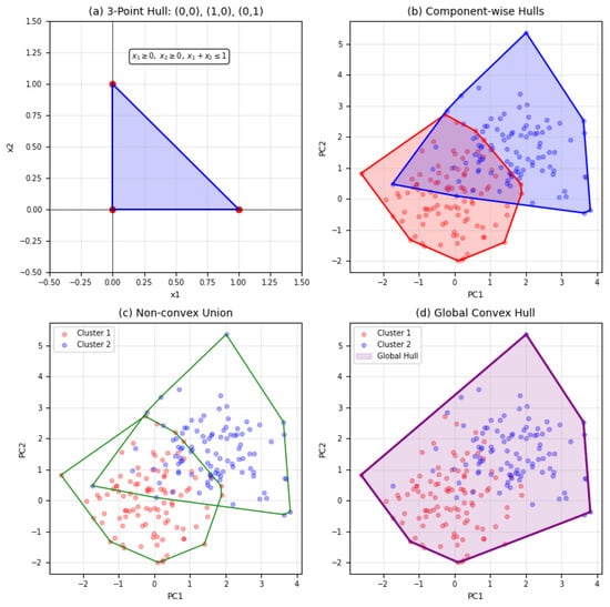
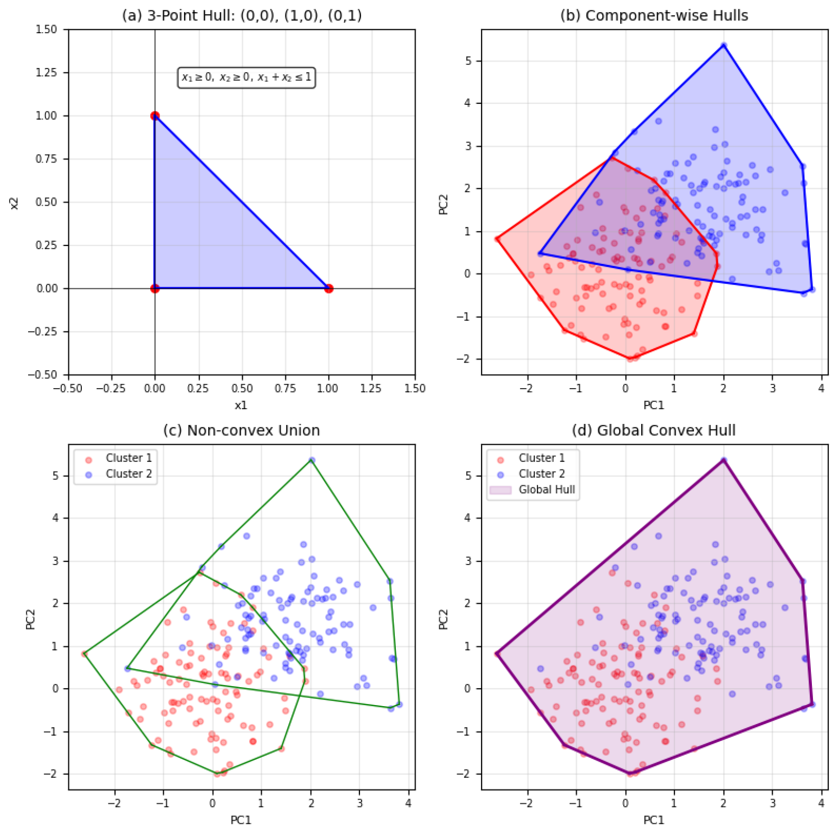
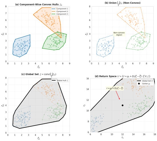
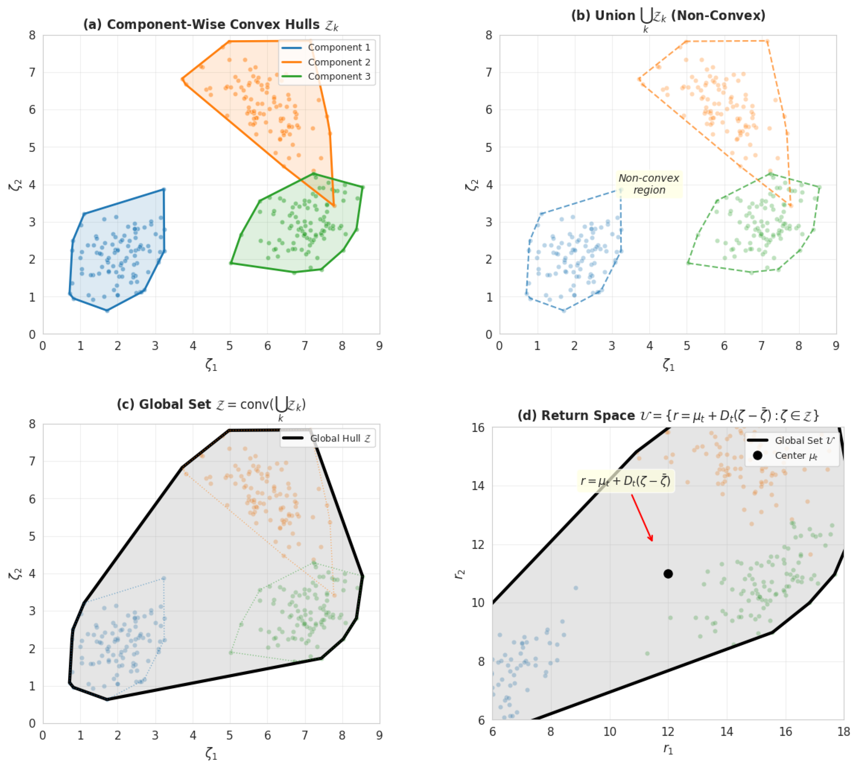
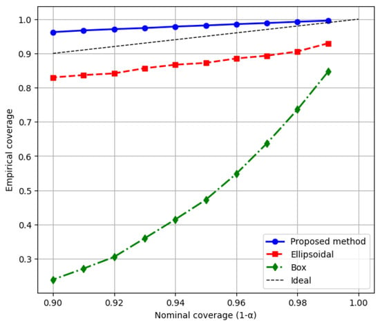
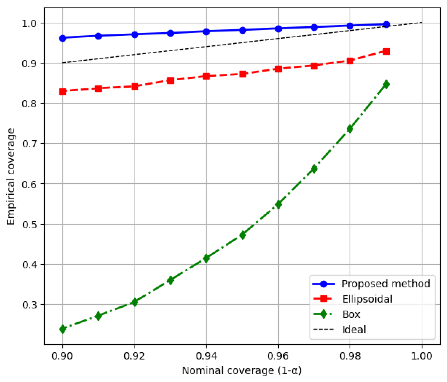
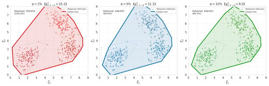
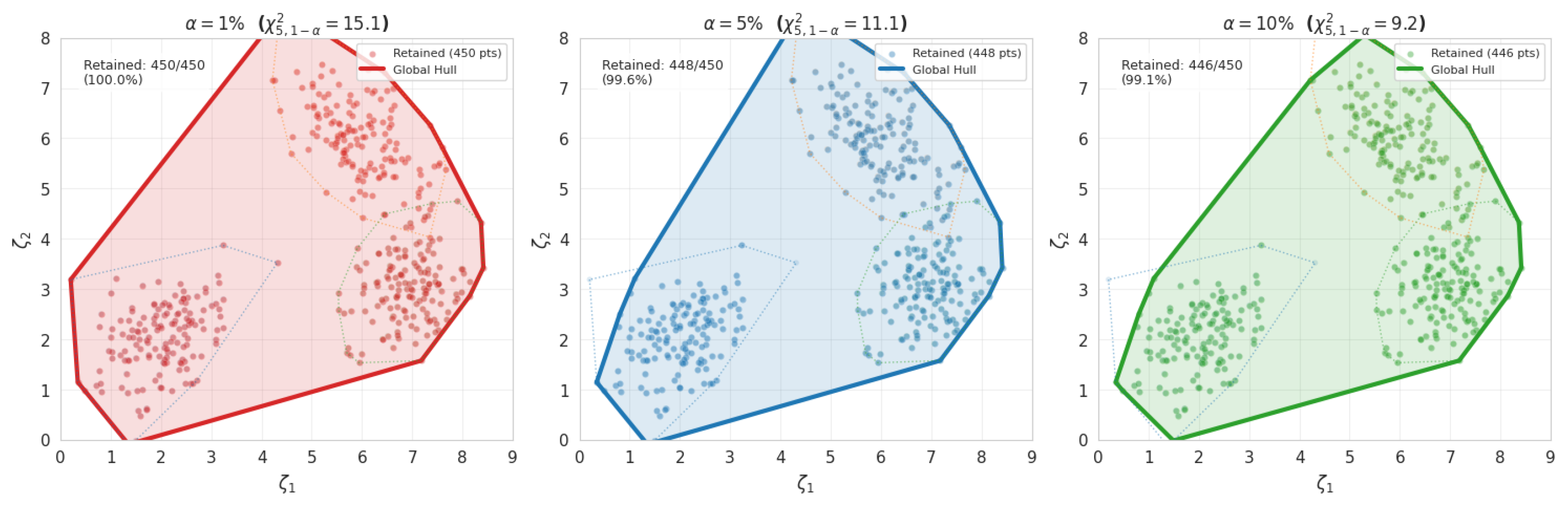
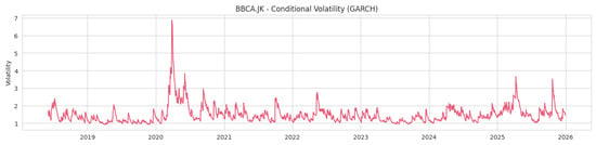
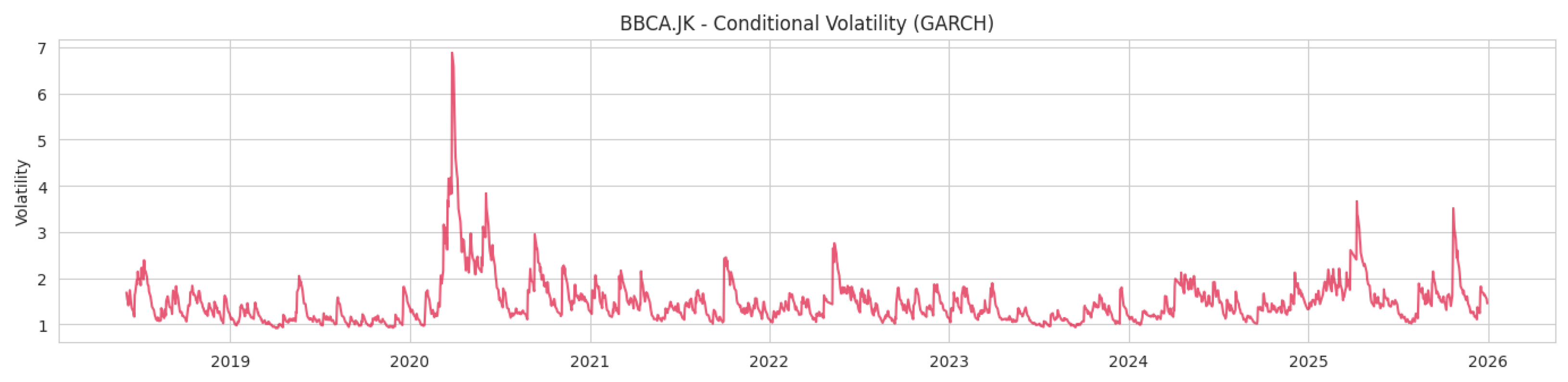
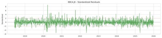
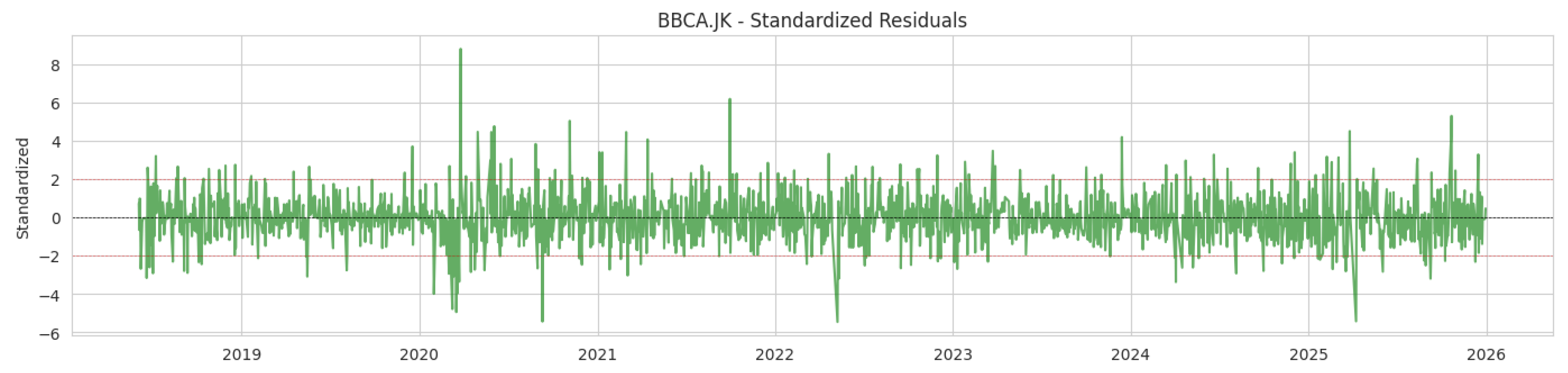
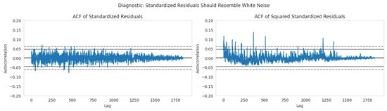
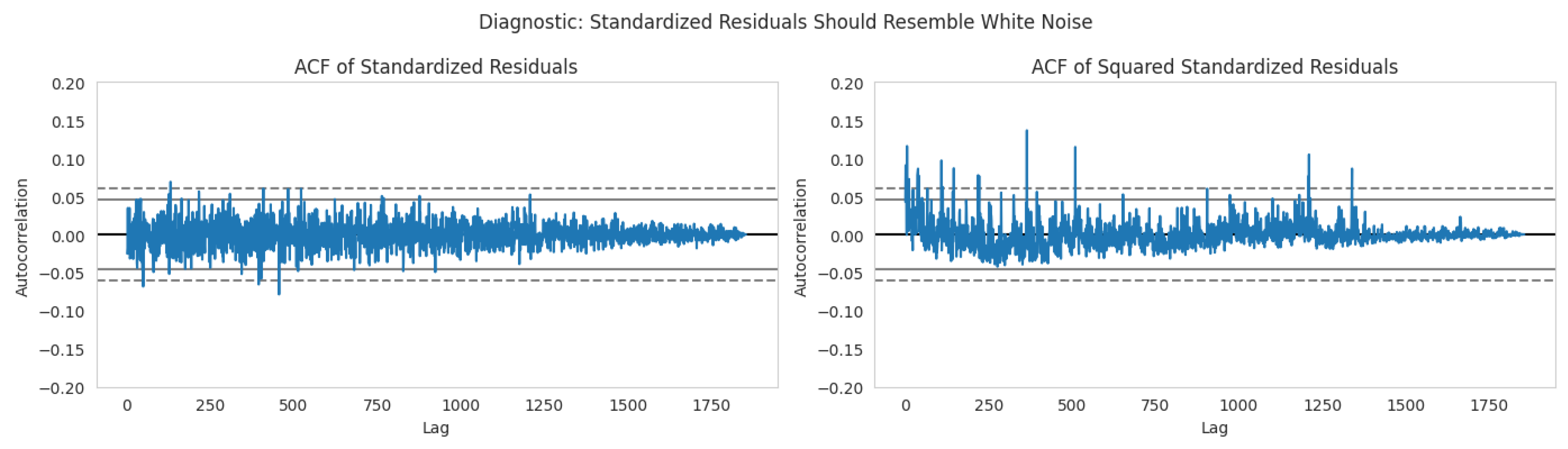
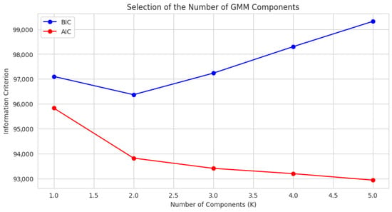
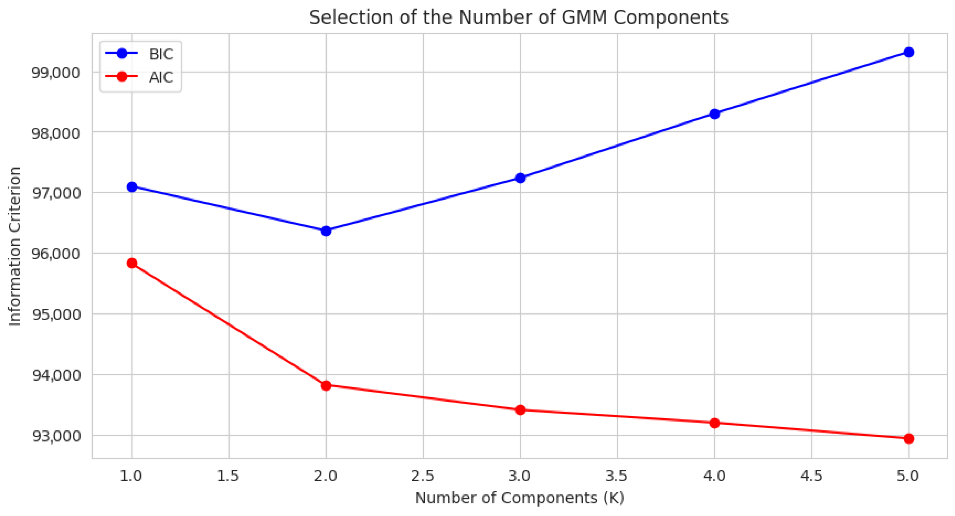
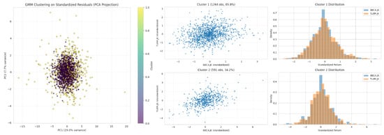
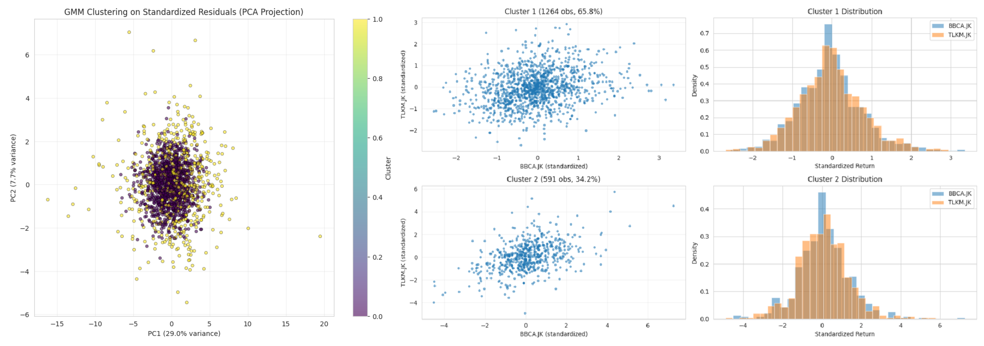
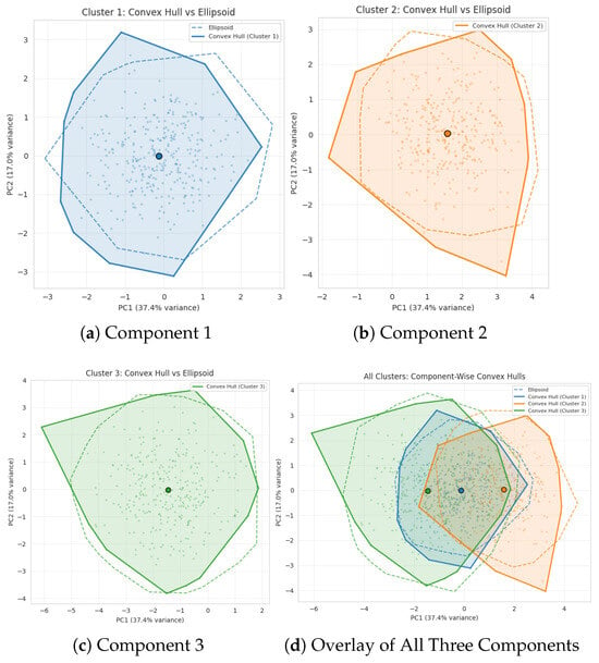
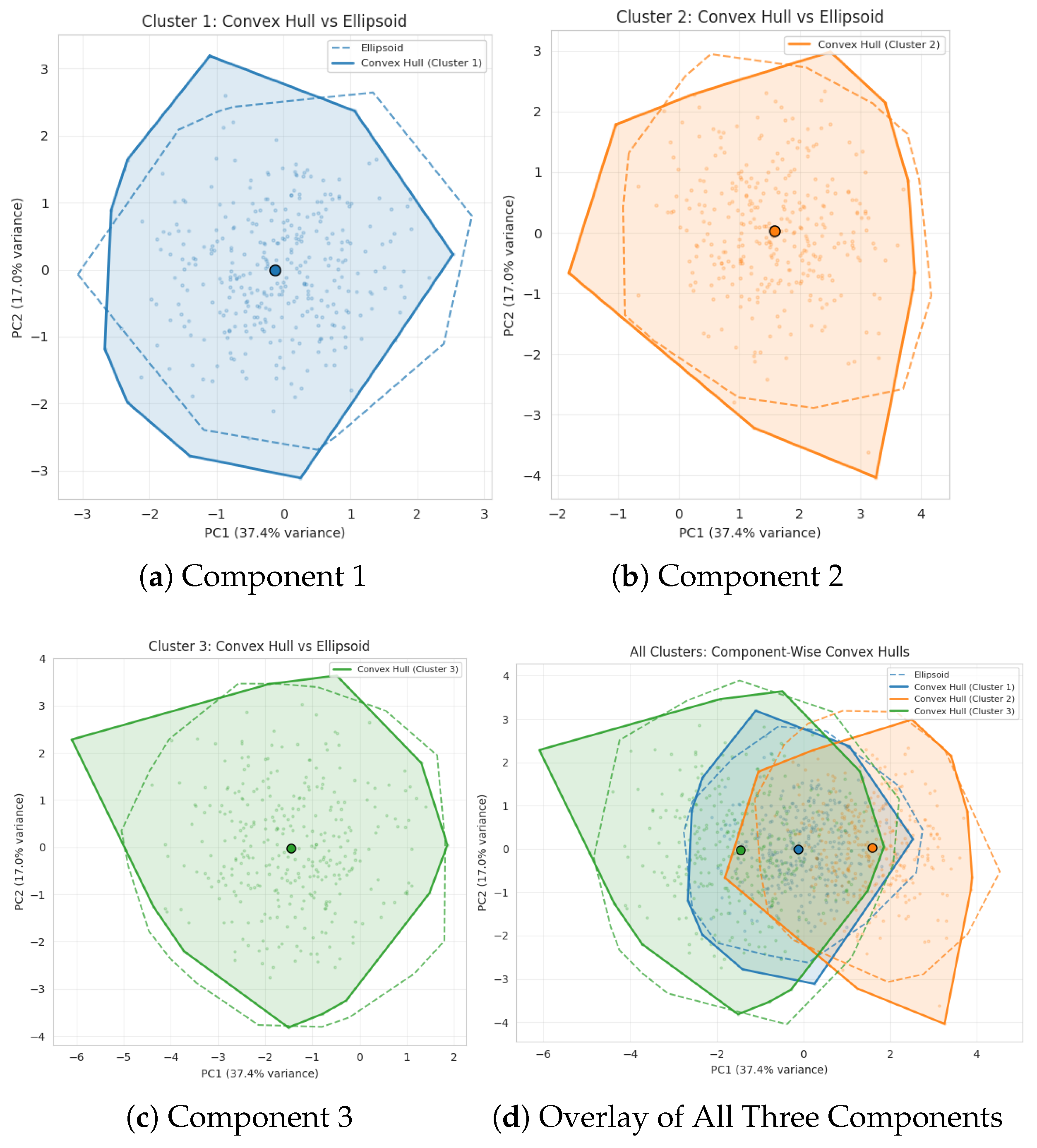
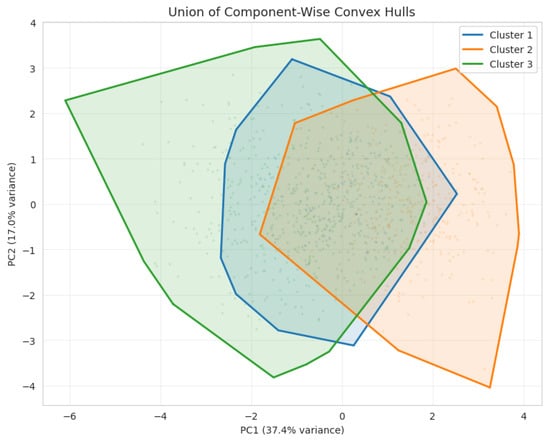
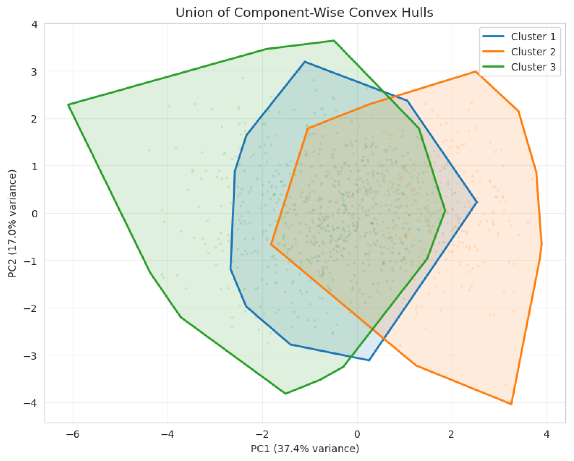
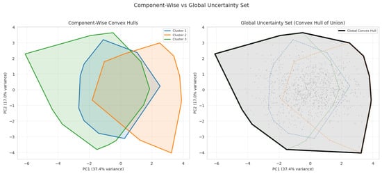
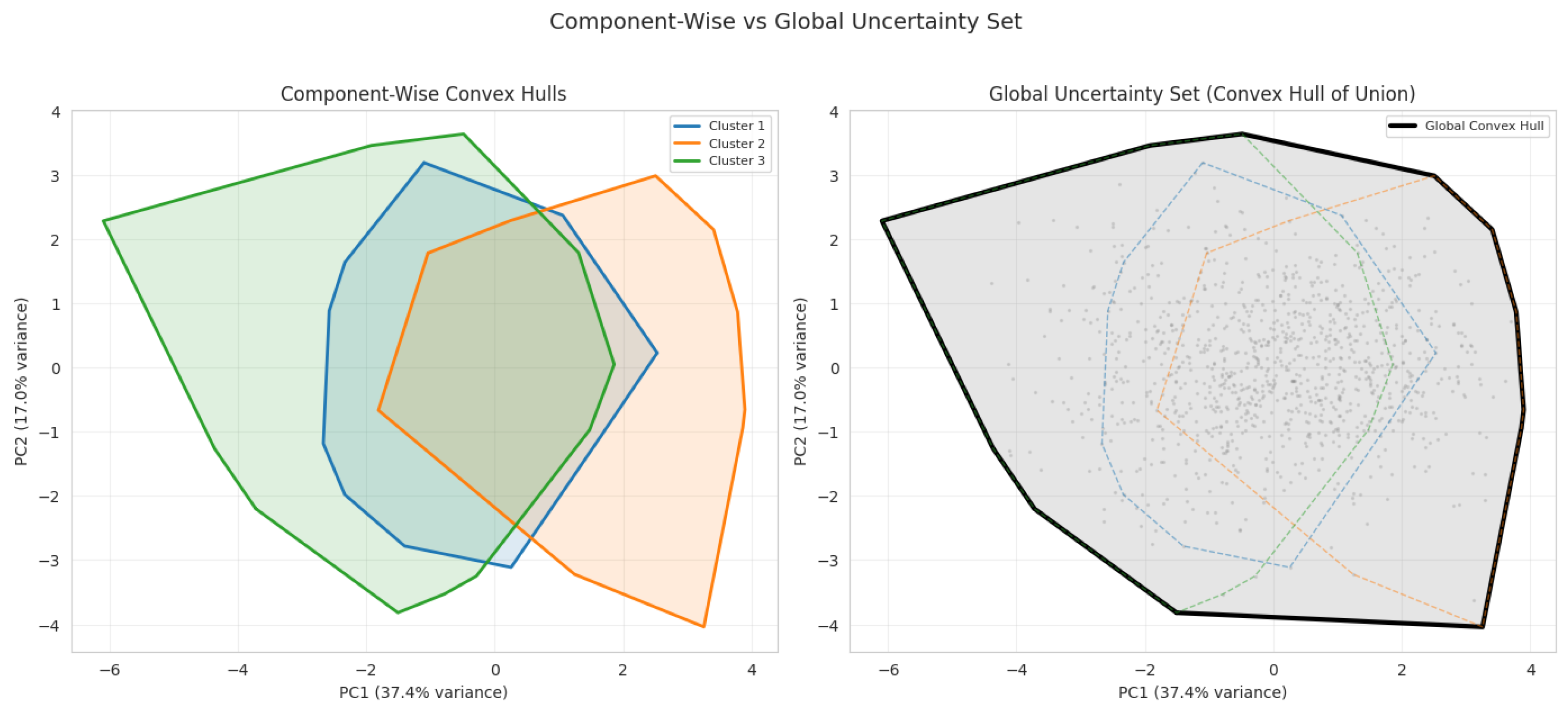
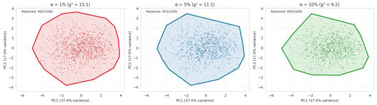
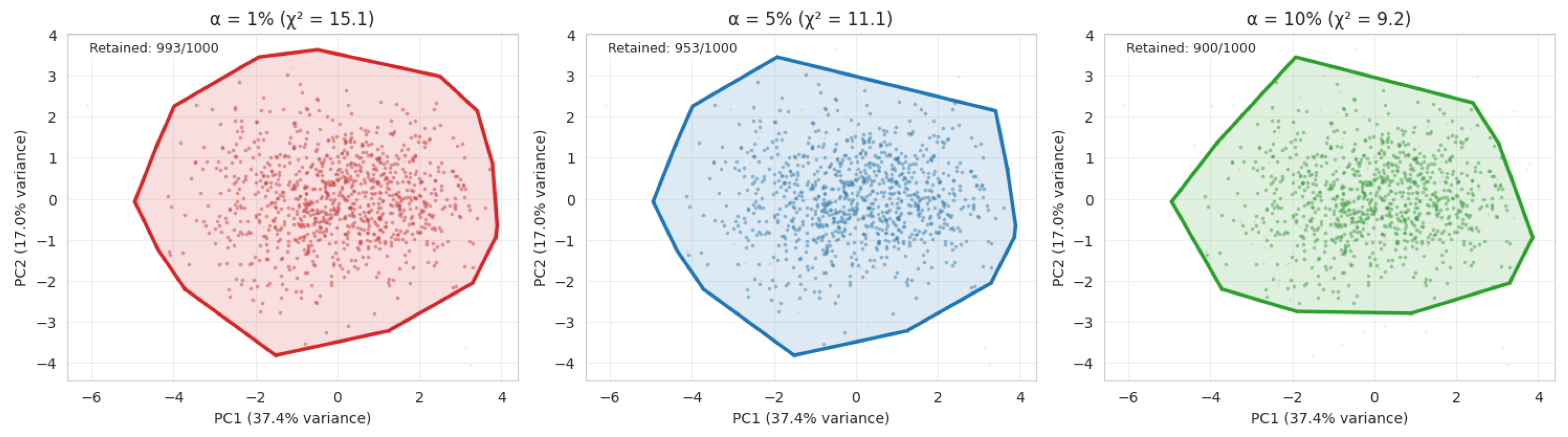
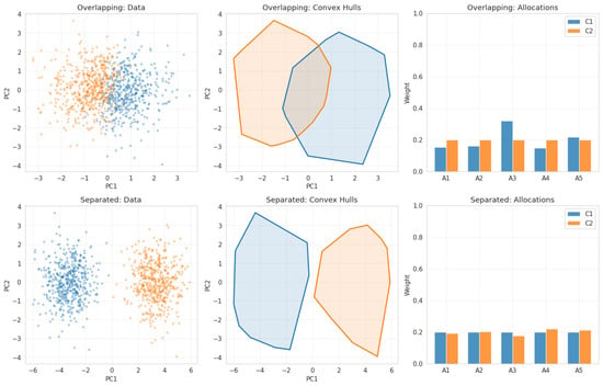
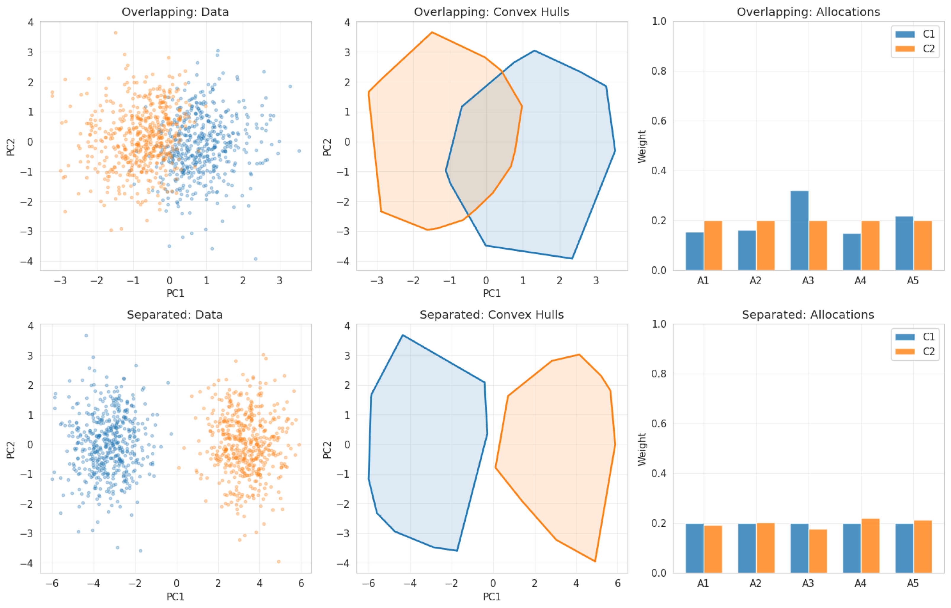
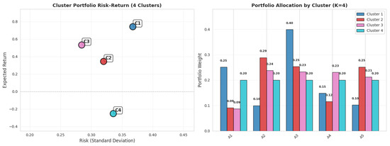
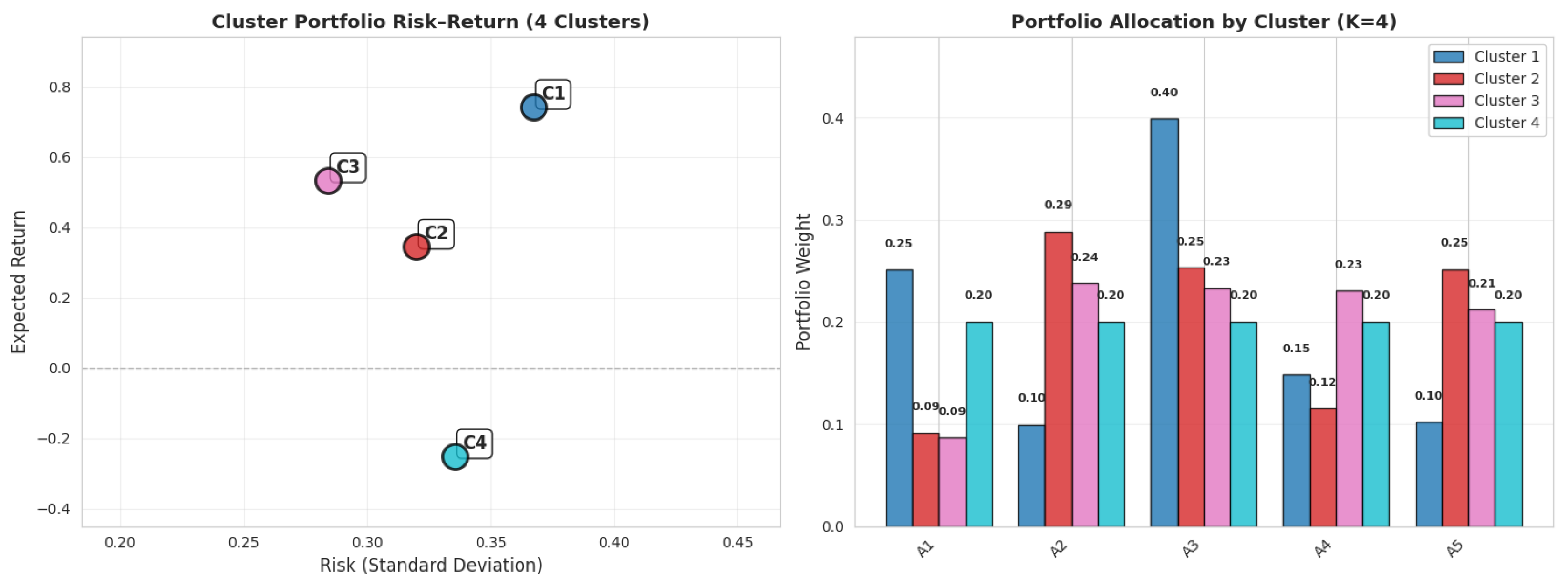
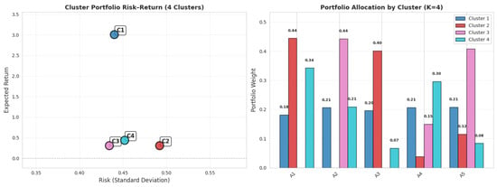
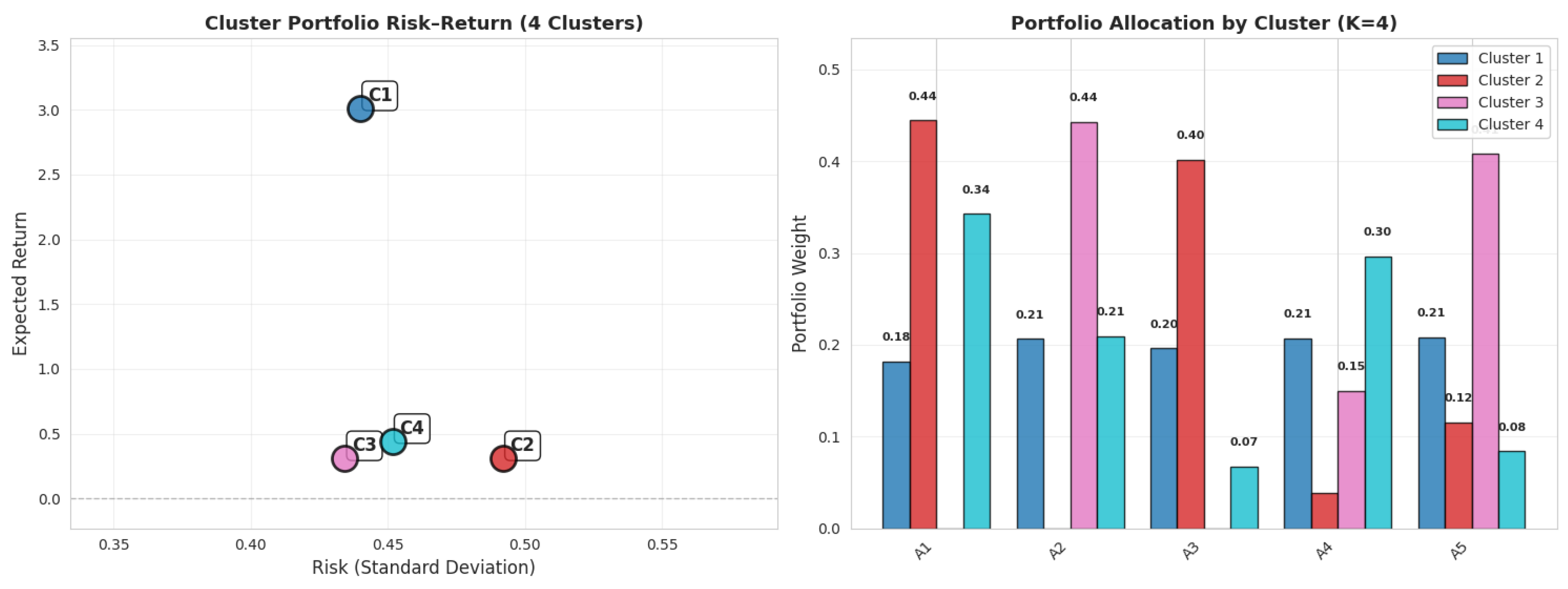
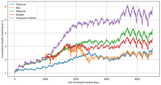
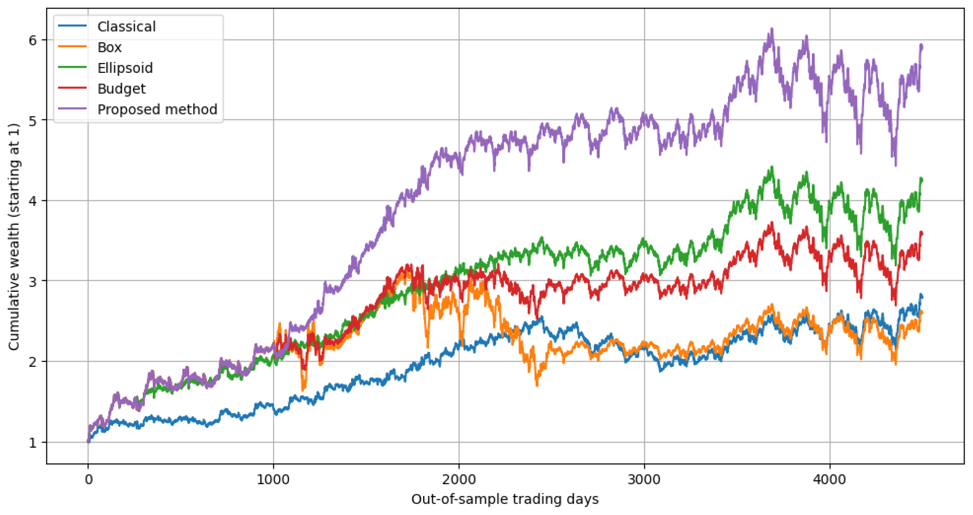
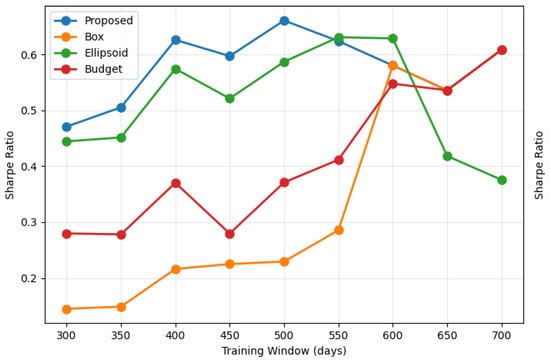
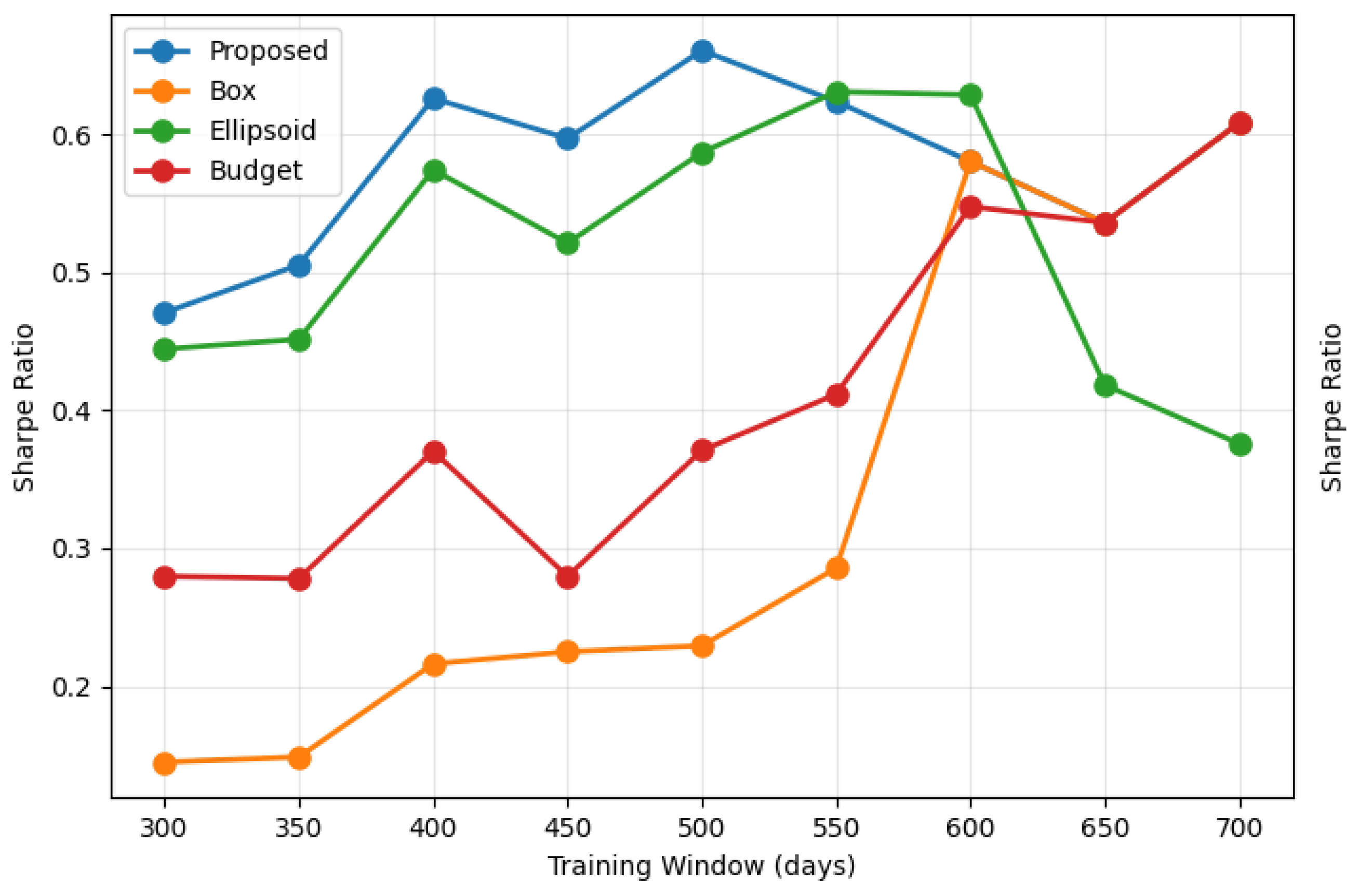
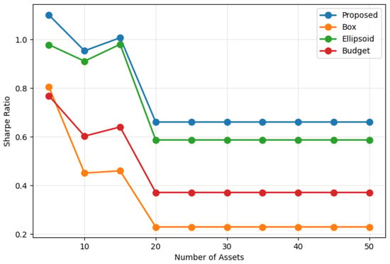
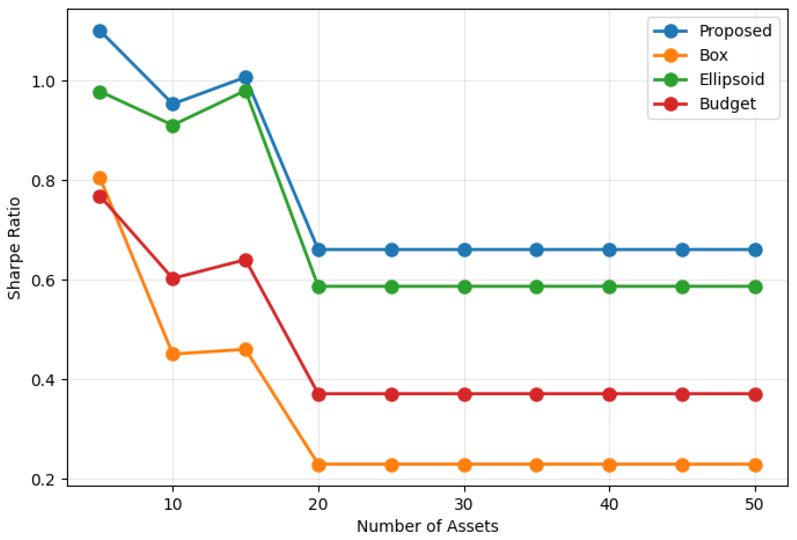
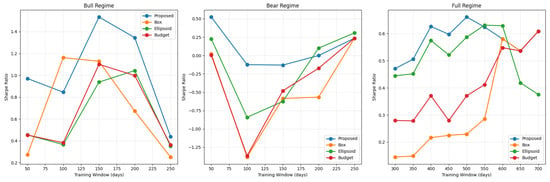
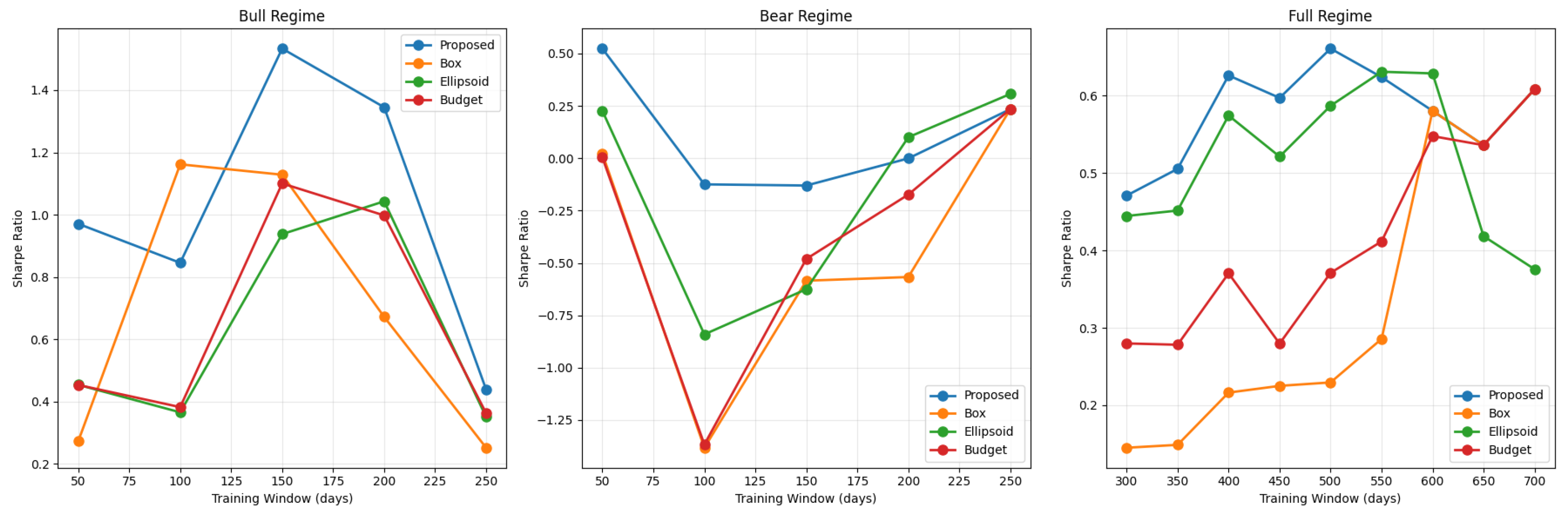
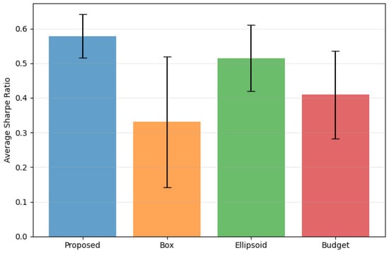
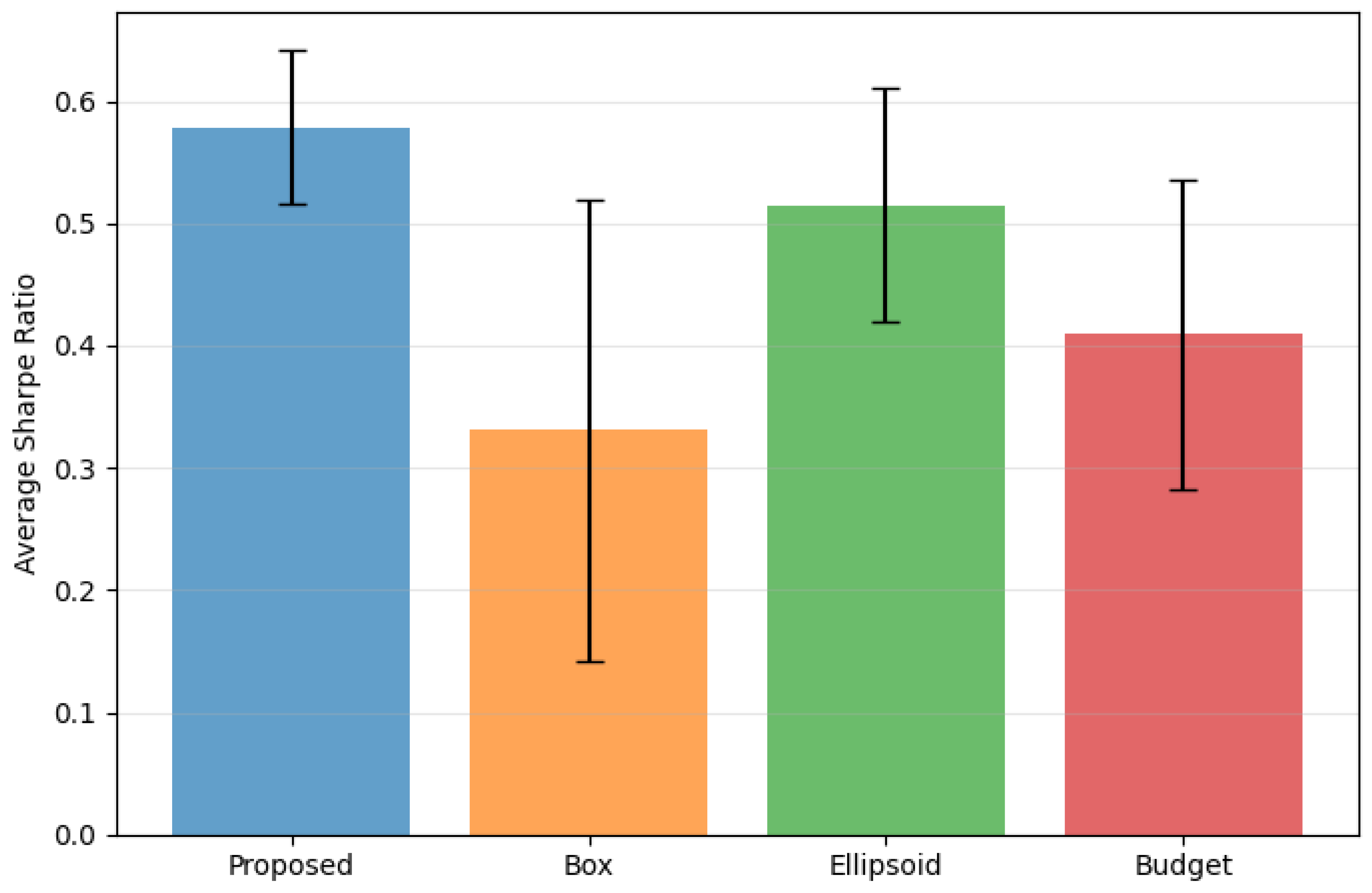

Disclaimer/Publisher’s Note: The statements, opinions and data contained in all publications are solely those of the individual author(s) and contributor(s) and not of MDPI and/or the editor(s). MDPI and/or the editor(s) disclaim responsibility for any injury to people or property resulting from any ideas, methods, instructions or products referred to in the content. |
© 2026 by the authors. Licensee MDPI, Basel, Switzerland. This article is an open access article distributed under the terms and conditions of the Creative Commons Attribution (CC BY) license.