Statistical Inference of the Mixed Exponential–Beta Distribution

Abstract

The classical exponential (Exp) distribution may have limited capability in describing asymmetric lifetime data and observations with different tail characteristics. In this paper, a new extended exponential model, called the Mixed Exponential–Beta (MEB) distribution, is proposed based on a scale-mixture representation involving exponential and beta distributions. The main statistical properties of the proposed distribution are investigated, including its probability density function (pdf), cumulative distribution function (cdf), reliability function, moments, skewness, and kurtosis. The additional shape parameters of the MEB distribution provide enhanced control over distributional shape, asymmetry, and tail behavior. The model parameters are estimated using the expectation–maximization (EM) algorithm based on the stochastic representation of the mixture model. The proposed EM-based maximum likelihood (ML) estimation method is further compared with the least-squares (LS) estimation method, and the results demonstrate its superior estimation accuracy. Finally, the applicability of the MEB distribution is illustrated through maintenance-time data, where the proposed model shows competitive fitting performance compared with several exponential-type distributions. The results indicate that the MEB distribution provides a flexible alternative for modeling positive lifetime data with different distributional characteristics. Moreover, the exponential distribution is obtained as a limiting case under appropriate parameter conditions.

1. Introduction

Scale-mixture models provide an effective statistical framework for accommodating heavy-tailed behavior and reducing the influence of atypical or extreme observations. Andrews and Mallows [1] introduced the scale-mixture representation of normal distributions and established necessary and sufficient conditions for a random variable of the form $X=Z/V$, where Z follows a standard normal distribution and is independent of V. Many classical statistical models assume normally distributed errors; however, such an assumption may be sensitive to extreme observations. To address this issue, heavy-tailed alternatives have been developed to improve robustness in the presence of outliers. For example, Choy et al. [2] constructed a heavy-tailed error model based on scale mixtures of normal distributions, providing an effective approach for statistical modeling in the presence of outliers.

Scale mixtures of skew normal distributions have also been extensively investigated. Zhou and Chen [3] proposed a class of scale-mixture skew normal distributions and evaluated the effectiveness of the proposed models through simulation studies and empirical applications involving comparisons among different mixture distributions. Kim and Hyoung-Moon [4] derived the first four moments of a skew normal scale-mixture random vector and obtained the first two moments of its quadratic form under a symmetric matrix, with further applications to second-order stationary time series. Xia and Liu [5] conducted a robust Bayesian analysis of a general factor analysis model based on normal scale mixtures to reduce the effects of distributional skewness and outliers on statistical inference.

In fields such as survival analysis, reliability engineering, and actuarial science, the exponential distribution is one of the most widely used lifetime distributions, and maximum likelihood (ML) estimation is commonly employed for parameter inference. Haq Muhammad Ahsan [6] proposed the Marshall–Olkin skewed exponential distribution and compared five different parameter estimation methods, with the results indicating favorable performance of the ML method among the considered procedures. Moshera A. M. Ahmad [7] derived the statistical properties of an exponential–inverse exponential Weibull regression failure model and obtained ML estimates of the model parameters based on censored data. Meanwhile, considerable attention has been devoted to extensions of the exponential distribution. Ruizheng Niu [8] systematically investigated discrimination among the generalized exponential distribution, weighted exponential (WE) distribution, and other weighted distributions. Wang et al. [9] constructed a four-parameter generalized exponential distribution, derived several of its statistical properties, including the probability density function, hazard function, and survival function, and thereby further enhanced the modeling flexibility of the exponential family.

However, existing models may exhibit limited fitting capacity for atypical and extreme observations, making it difficult to fully accommodate complex data structures. To address this issue, various extensions of the exponential distribution have been proposed. Among them, the Weibull distribution and generalized exponential (GE) distribution have received extensive attention, as summarized by Gupta and Kundu [10,11,12]. The generalized mixed exponential (GME) distribution proposed by Yang, Tian, and Tong [13] further enriches the existing modeling framework. It includes the exponential and Weibull distributions as special cases, thereby improving its applicability. Barahona et al. [14] developed a scale-mixture exponential (SME) model by combining an exponential distribution with a beta mixing distribution. Nevertheless, existing models may still have limited flexibility in controlling kurtosis and describing data containing extreme observations. Motivated by these considerations, the present study extends the exponential–beta mixture framework and proposes a new extended exponential distribution, referred to as the MEB distribution.

In particular, the SME distribution proposed by Barahona et al. [14] is constructed using a symmetric beta $(q,q)$ mixing variable. The model proposed in the present paper replaces this symmetric mixing distribution with the more general beta $(\alpha ,\beta )$ distribution. Consequently, the SME distribution is nested in the proposed MEB family as the special case $\alpha =\beta =q$. The two distinct shape parameters of the beta mixing distribution independently control its behavior near the boundaries 0 and 1. This additional degree of flexibility enables the MEB distribution to accommodate a wider range of tail behavior and asymmetric shapes.

This study systematically investigates the proposed Mixed Exponential–Beta distribution, including its probabilistic properties, moment characteristics, reliability measures, parameter estimation procedure, and practical modeling performance. The scale-mixture representation provides a flexible mechanism for describing positively skewed observations and data exhibiting pronounced right-tail behavior. In addition, maximum likelihood estimation is developed through an EM algorithm, and the finite-sample performance of the resulting estimators is investigated through Monte Carlo simulation.

The remainder of this paper is organized as follows. Section 2 introduces the MEB distribution and derives its main statistical properties. Section 3 develops the maximum likelihood estimation procedure based on the EM algorithm and evaluates its finite-sample performance through Monte Carlo simulations. Section 4 presents an application to maintenance-time data and compares the proposed model with several competing lifetime distributions. Finally, Section 5 concludes the paper.

2. Definition and Statistical Properties of the MEB Distribution

2.1. Construction and Probabilistic Properties of the MEB Distribution

Definition 1

([15]). The integral definition of the confluent hypergeometric function is given by

$$M(a,b;x)={\displaystyle \frac{\mathsf{\Gamma }\left(b\right)}{\mathsf{\Gamma }\left(a\right)\mathsf{\Gamma }(b-a)}}{\int }_0^1{v}^{a-1}{(1-v)}^{b-a-1}{e}^{xv}dv,b>a>0.$$

(1)

Definition 2

([15]). The expression for the Gauss hypergeometric function is given by

$$\begin{array}{cc}\hfill F(a,b,c;x)& ={\displaystyle \frac{\mathsf{\Gamma }\left(c\right)}{\mathsf{\Gamma }\left(b\right)\mathsf{\Gamma }(c-b)}}{\int }_0^1{v}^{b-1}{(1-v)}^{c-b-1}{(1-xv)}^{-a}dv,\hfill \end{array}$$

(2)

where $c>a+b$ or $a+b-1<c\le a+b$.

Definition 3.

If a random variable $Z(Z>0)$ has a pdf of the form

$$f_Z(z;\lambda ,\alpha ,\beta )=2\lambda e^{-2\lambda z}{\displaystyle \frac{\alpha }{\alpha +\beta }}M(\beta ,\alpha +\beta +1;2\lambda z),$$

(3)

where $\lambda >0$ is the scale parameter, $\alpha ,\beta >0$ are the shape parameters, and $M(a,b;x)$ is the confluent hypergeometric function. Then Z is said to follow the Mixed Exponential–Beta distribution, denoted by $Z\sim \mathit{MEB}(\lambda ,\alpha ,\beta )$.

Remark 1.

When $\alpha =\beta =q$, the MEB distribution reduces to the SME distribution proposed by Barahona et al. [14]. Therefore, the SME distribution is a nested submodel of the proposed MEB family.

Proposition 1.

Let X, Z be random variables, $Z|X=x\sim E(2\lambda x),X\sim \mathit{Beta}(\alpha ,\beta )$, then $Z\sim \mathit{MEB}(\lambda ,\alpha ,\beta )$.

Proof. 

According to the scale mixture property, beta function, gamma function and Equation (1), which is given by

$$\begin{array}{cc}\hfill f_Z\left(z\right)& ={\int }_0^1{f}_{Z|X}\left(z\right)f_X\left(x\right)dx\hfill \\ \hfill & ={\int }_0^{1}2\lambda x{e}^{-2\lambda xz}{\displaystyle \frac{1}{B(\alpha ,\beta )}}{x}^{\alpha -1}{(1-x)}^{\beta -1}dx\hfill \\ \hfill & ={\displaystyle \frac{2\lambda }{B(\alpha ,\beta )}}{\int }_0^1{x}^{\alpha }{(1-x)}^{\beta -1}{e}^{-2\lambda zx}dx\hfill \\ \hfill & ={\displaystyle \frac{2\lambda e^{-2\lambda z}}{B(\alpha ,\beta )}}·{\displaystyle \frac{\mathsf{\Gamma }\left(\beta \right)\mathsf{\Gamma }(\alpha +1)}{\mathsf{\Gamma }(\alpha +\beta +1)}}M(\beta ,\alpha +\beta +1;2\lambda z)\hfill \\ \hfill & =2\lambda e^{-2\lambda z}{\displaystyle \frac{\alpha }{\alpha +\beta }}M(\beta ,\alpha +\beta +1;2\lambda z).\hfill \end{array}$$

□

Proposition 2.

Suppose that random variables $X\sim \mathit{Exp}\left(\lambda \right)$, $Y\sim \mathit{beta}(\alpha ,\beta )$, and X is independent of Y, then $Z={\displaystyle \frac{X}{2Y}}\sim \mathit{MEB}(\lambda ,\alpha ,\beta )$.

Proof. 

By using the variable transformation method with the Jacobian matrix, we have

$$\left.\begin{array}{cc}\hfill Z& ={\displaystyle \frac{X}{2Y}}\hfill \\ \hfill V& =Y\hfill \end{array}\right\}\Rightarrow \left.\begin{array}{cc}\hfill X& =2ZV\hfill \\ \hfill Y& =V\hfill \end{array}\right\}\Rightarrow J=\left|\begin{array}{cc}{\displaystyle \frac{\partial x}{\partial z}}& {\displaystyle \frac{\partial x}{\partial v}}\\ {\displaystyle \frac{\partial y}{\partial z}}& {\displaystyle \frac{\partial y}{\partial v}}\end{array}\right|=\left|\begin{array}{cc}2v& 2z\\ 0& 1\end{array}\right|=2v,$$

it follows that

$$\begin{array}{cc}\hfill f_{Z,V}(z,v)& =\left|J\right|f_{X,Y}(2zv,v)\hfill \\ \hfill & =2v{f}_X\left(2zv\right)f_Y\left(v\right)\hfill \\ \hfill & ={\displaystyle \frac{2v^{\alpha }\lambda e^{-2\lambda zv}{(1-v)}^{\beta -1}}{B(\alpha ,\beta )}},\hfill \end{array}$$

where 0 < v < 1 and $z>0$. Marginalizing with respect to V, we obtain the pdf of Z is given by

$$\begin{array}{cc}\hfill f_Z(z;\lambda ,\alpha ,\beta )& ={\displaystyle \frac{2\lambda }{B(\alpha ,\beta )}}{\int }_0^1{v}^{\alpha }{(1-v)}^{\beta -1}{e}^{-2z\lambda v}dv\hfill \\ \hfill & =2\lambda e^{-2\lambda z}{\displaystyle \frac{\alpha }{\alpha +\beta }}M(\beta ,\alpha +\beta +1;2\lambda z).\hfill \end{array}$$

□

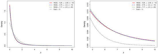
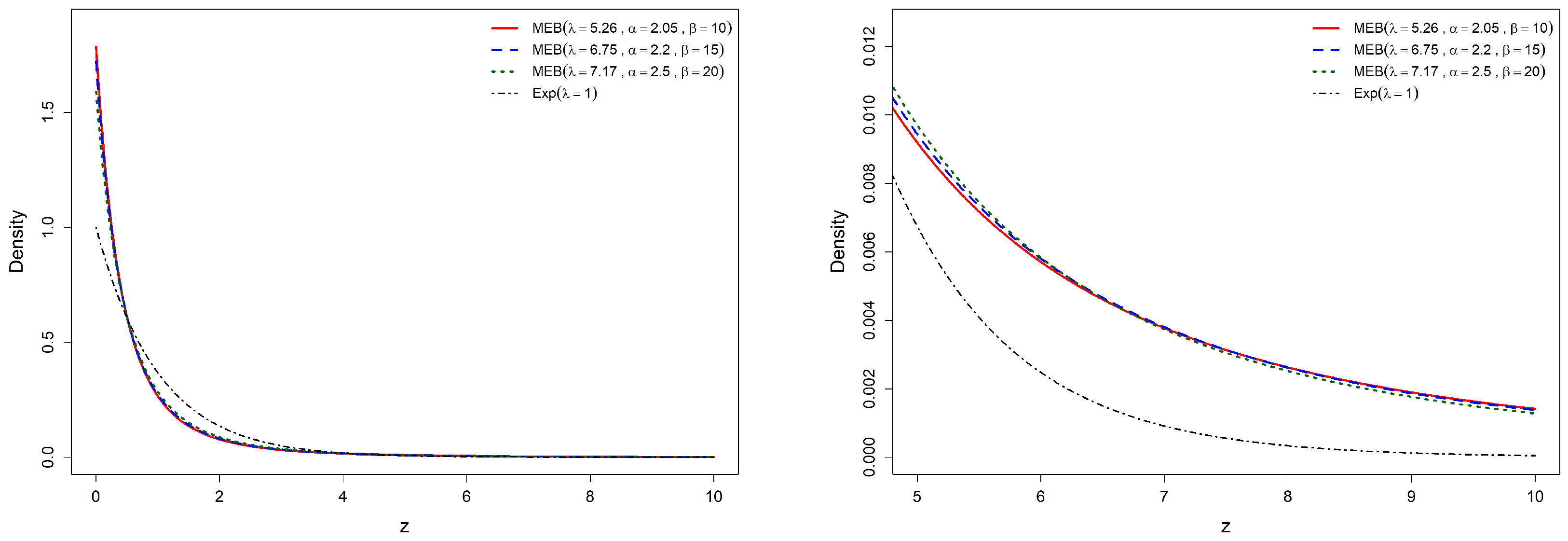
To examine the shape characteristics of the proposed MEB distribution, we compare its pdfs under different parameter settings with the pdf of the an Exp distribution with rate 1 distribution under a common-mean constraint, as shown in Figure 1.

Figure 1. Comparison of density MEB and Exp(1) distributions.

It should be noted that Figure 1 is constructed under a common-mean constraint. Therefore, the value of $\lambda$ is adjusted simultaneously when different combinations of $\alpha$ and $\beta$ are considered. This joint adjustment can partially offset the changes in the shape parameters and may cause the central parts of some density curves to appear relatively similar.

However, the differences between the parameter settings become more visible in the right-tail region. As shown in the enlarged panel of Figure 1 and in the numerical tail probabilities reported in Table 1, different combinations of $\alpha$ and $\beta$ produce noticeably different tail behavior even when the distributions are compared under the same mean condition. A more detailed analytical interpretation of the separate roles of $\alpha$ and $\beta$ is provided later through the reliability, moment, skewness, and kurtosis properties of the MEB distribution.

Table 1. Comparison of tail probabilities between the MEB distribution with different parameter settings and the Exp(1) distribution under the same mean condition.

Distribution	$\mathit{P}\mathbf{(}\mathit{Z}\mathbf{>}\mathbf{3}\mathbf{)}$	$\mathit{P}\mathbf{(}\mathit{Z}\mathbf{>}\mathbf{4}\mathbf{)}$	$\mathit{P}\mathbf{(}\mathit{Z}\mathbf{>}\mathbf{8}\mathbf{)}$
Exp(1)	0.04979	0.01832	0.00034
MEB (5.26, 2.05, 10)	0.06167	0.03870	0.01138
MEB (6.75, 2.2, 15)	0.06262	0.03872	0.01078
MEB (7.17, 2.5, 20)	0.06324	0.03789	0.00943

Although the density curves under the common-mean constraint may exhibit similar central behavior, the differences among parameter settings become more evident in terms of tail probability, skewness, kurtosis, and hazard-rate characteristics.

This indicates that the proposed model can provide greater flexibility in describing right-tail behavior under the considered parameter settings.

2.2. MEB Cumulative Distribution Function

Proposition 3.

Let $Z\sim \mathrm{MEB}(\lambda ,\alpha ,\beta )$, then the cdf is given by

$$F_Z(z;\lambda ,\alpha ,\beta )=1-e^{-2\lambda z}M(\beta ,\alpha +\beta ;2\lambda z),$$

(4)

where $z>0$, and $\lambda >0,\alpha >0,\beta >0$ are parameters.

Proof. 

From the integral definition of the confluent hypergeometric function, it follows that

$$\begin{array}{cc}\hfill F_Z(z;\lambda ,\alpha ,\beta )& ={\int }_0^{z}2\lambda {\displaystyle \frac{\alpha }{\alpha +\beta }}{e}^{-2\lambda t}M\left(\beta ,\alpha +\beta +1;2\lambda t\right)dt\hfill \\ \hfill & ={\displaystyle \frac{2\lambda }{B(\alpha ,\beta )}}{\int }_0^1{v}^{\beta -1}{(1-v)}^{\alpha }\left({\int }_0^z{e}^{-2\lambda t(1-v)}dt\right)dv\hfill \\ \hfill & ={\displaystyle \frac{1}{B(\alpha ,\beta )}}{\int }_0^1{v}^{\beta -1}{(1-v)}^{\alpha -1}\left[1-e^{-2\lambda z(1-v)}\right]dv\hfill \\ \hfill & =1-{\displaystyle \frac{e^{-2\lambda z}}{B(\alpha ,\beta )}}{\int }_0^1{v}^{\beta -1}{(1-v)}^{\alpha -1}{e}^{2\lambda zv}dv\hfill \\ \hfill & =1-e^{-2\lambda z}M\left(\beta ,\alpha +\beta ;2\lambda z\right).\hfill \end{array}$$

□

2.3. Reliability Analysis

Corollary 1.

Let $T\sim \mathit{MEB}(\lambda ,\alpha ,\beta )$, $r\left(t\right)$ be the reliability function, and $h\left(t\right)$ be the hazard function. Then the corresponding expressions are given by

$$\begin{array}{cc}\hfill r\left(t\right)& =e^{-2\lambda t}M\left(\beta ,\alpha +\beta ;2\lambda t\right),\hfill \\ \hfill h\left(t\right)& ={\displaystyle \frac{2\lambda \alpha }{\alpha +\beta }}{\displaystyle \frac{M\left(\beta ,\alpha +\beta +1;2\lambda t\right)}{M\left(\beta ,\alpha +\beta ;2\lambda t\right)}}.\hfill \end{array}$$

Proof. 

Clearly

$$\begin{array}{cc}\hfill r\left(t\right)& =1-F\left(t\right)=e^{-2\lambda t}M\left(\beta ,\alpha +\beta ;2\lambda t\right),\hfill \\ \hfill h\left(t\right)& ={\displaystyle \frac{f\left(t\right)}{r\left(t\right)}}\hfill \\ \hfill & ={\displaystyle \frac{2\lambda e^{-2\lambda t}{\displaystyle \frac{\alpha }{\alpha +\beta }}M\left(\beta ,\alpha +\beta +1;2\lambda t\right)}{e^{-2\lambda t}M\left(\beta ,\alpha +\beta ;2\lambda t\right)}}\hfill \\ \hfill & ={\displaystyle \frac{2\lambda \alpha }{\alpha +\beta }}{\displaystyle \frac{M\left(\beta ,\alpha +\beta +1;2\lambda t\right)}{M\left(\beta ,\alpha +\beta ;2\lambda t\right)}}.\hfill \end{array}$$

where $f\left(t\right)$ denotes the pdf, and $F\left(t\right)$ the cdf of the MEB distribution. □

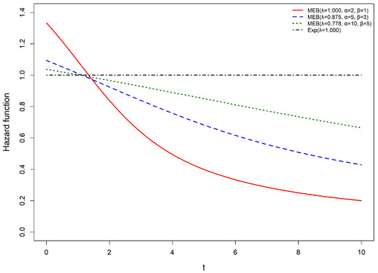
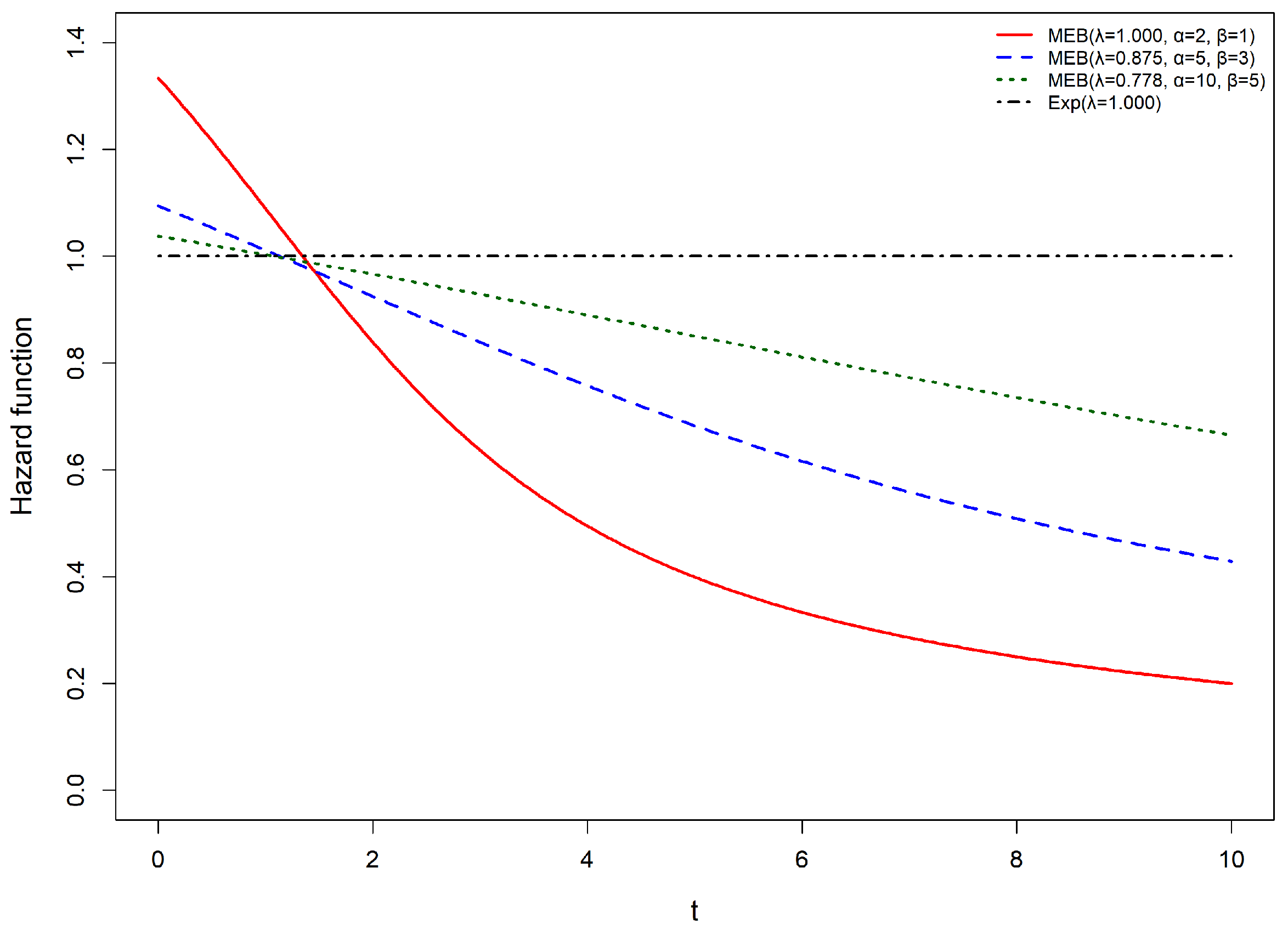
To further examine the reliability characteristics of the proposed model, hazard functions of the MEB distribution with different parameter settings are compared with the Exp(1) distribution under the same mean condition, the results are shown in Figure 2.

Figure 2. Comparison of hazard functions between the MEB distribution under different parameter settings and the Exp(1) distribution.

Figure 2 provides a numerical illustration of the hazard-rate behavior of the proposed MEB distribution under different parameter settings. Under the same mean constraint, the selected MEB hazard functions exhibit decreasing patterns over time, while the Exp(1) distribution has a constant hazard rate. The different shapes of the hazard curves demonstrate that the additional parameters of the MEB distribution provide greater flexibility in modeling various failure-rate behaviors.

Therefore, compared with the exponential distribution, the proposed MEB distribution can accommodate a wider range of hazard-rate patterns, which is beneficial for modeling lifetime data with different characteristics.

2.4. Order Statistic

From the pdf of order statistics, we derive the following corollary.

Corollary 2.

Let $Z_1,Z_2,\dots ,Z_n$ be independent and identically distributed random variables following the $\mathrm{MEB}(\lambda ,\alpha ,\beta )$ distribution, and let $Z_{\left(1\right)},Z_{\left(2\right)},\dots ,Z_{\left(n\right)}$ denote the corresponding order statistics. Then the pdf of the k-th order statistic is given by

$$\begin{array}{cc}\hfill f_{Z_{\left(k\right)}}\left(y\right)=& {\displaystyle \frac{n!}{(k-1)!(n-k)!}}{\left[1-e^{-2\lambda y}M\left(\beta ,\alpha +\beta ;2\lambda y\right)\right]}^{k-1}\hfill \\ \hfill & \times {\left[e^{-2\lambda y}M\left(\beta ,\alpha +\beta ;2\lambda y\right)\right]}^{n-k}\hfill \\ \hfill & \times 2\lambda {\displaystyle \frac{\alpha }{\alpha +\beta }}{e}^{-2\lambda y}M\left(\beta ,\alpha +\beta +1;2\lambda y\right),y>0.\hfill \end{array}$$

(5)

Therefore, the pdf of the maximum order statistic $Z_{\left(n\right)}$ is given by

$$\begin{array}{cc}\hfill f_{Z_{\left(n\right)}}\left(y\right)=& 2\lambda n{\displaystyle \frac{\alpha }{\alpha +\beta }}{e}^{-2\lambda y}M\left(\beta ,\alpha +\beta +1;2\lambda y\right)\hfill \\ \hfill & \times {\left[1-e^{-2\lambda y}M\left(\beta ,\alpha +\beta ;2\lambda y\right)\right]}^{n-1},y>0.\hfill \end{array}$$

(6)

The pdf of the minimum order statistic $Z_{\left(1\right)}$ is given by

$$\begin{array}{cc}\hfill f_{Z_{\left(1\right)}}\left(y\right)=& 2\lambda n{\displaystyle \frac{\alpha }{\alpha +\beta }}{e}^{-2\lambda y}M\left(\beta ,\alpha +\beta +1;2\lambda y\right)\hfill \\ \hfill & \times {\left[e^{-2\lambda y}M\left(\beta ,\alpha +\beta ;2\lambda y\right)\right]}^{n-1},y>0.\hfill \end{array}$$

(7)

Proof. 

For a random sample from an absolutely continuous distribution with pdf $f_Z\left(y\right)$ and cdf $F_Z\left(y\right)$, the standard density of the k-th order statistic is

$$f_{Z_{\left(k\right)}}\left(y\right)={\displaystyle \frac{n!}{(k-1)!(n-k)!}}{\left[F_Z\left(y\right)\right]}^{k-1}{\left[1-F_Z\left(y\right)\right]}^{n-k}{f}_Z\left(y\right).$$

Substituting the pdf in Equation (3) and the cdf in Equation (4) into the standard order-statistic density formula gives

$$\begin{array}{cc}\hfill f_{Z_{\left(k\right)}}\left(y\right)=& {\displaystyle \frac{n!}{(k-1)!(n-k)!}}{\left[1-e^{-2\lambda y}M\left(\beta ,\alpha +\beta ;2\lambda y\right)\right]}^{k-1}\hfill \\ \hfill & \times {\left[e^{-2\lambda y}M\left(\beta ,\alpha +\beta ;2\lambda y\right)\right]}^{n-k}\hfill \\ \hfill & \times 2\lambda {\displaystyle \frac{\alpha }{\alpha +\beta }}{e}^{-2\lambda y}M\left(\beta ,\alpha +\beta +1;2\lambda y\right),y>0,\hfill \end{array}$$

which gives Equation (5).

Taking $k=n$, we obtain Equation (6)

Similarly, taking $k=1$, we obtain Equation (7)

This completes the proof. □

2.5. Limiting Behavior

Proposition 4.

Let $Z\sim \mathrm{MEB}(\lambda ,\alpha ,\beta )$, if $\alpha ,\beta \to \infty$ with $\alpha /\beta \to 1$, then Z converges in law to an exponential distribution with parameter λ.

Proof. 

Let $Z=X/2Y$, where $X\sim \mathrm{Exp}\left(\lambda \right)$ and $Y\sim \beta (\alpha ,\beta )$. Under the assumptions $\alpha ,\beta \to \infty$ and $\alpha /\beta \to 1$, we have

$$\mathbb{E}\left[Y\right]={\displaystyle \frac{\alpha }{\alpha +\beta }}\to {\displaystyle \frac{1}{2}},$$

and

$$\mathrm{Var}\left[Y\right]={\displaystyle \frac{\alpha \beta }{{(\alpha +\beta )}^2(\alpha +\beta +1)}}\le {\displaystyle \frac{1}{4(\alpha +\beta +1)}}\to 0,$$

by Chebyshev’s inequality, for every $ϵ>0$, we have

$$\begin{array}{cc}\hfill P\left(\left|Y-{\displaystyle \frac{1}{2}}\right|>ϵ\right)& \le P\left(\left|Y-E\left[Y\right]\right|>{\displaystyle \frac{ϵ}{2}}\right)+P\left(\left|E\left[Y\right]-{\displaystyle \frac{1}{2}}\right|>{\displaystyle \frac{ϵ}{2}}\right)\hfill \\ \hfill & \le {\displaystyle \frac{4\mathrm{Var}\left(Y\right)}{{ϵ}^2}}+P\left(\left|E\left[Y\right]-{\displaystyle \frac{1}{2}}\right|>{\displaystyle \frac{ϵ}{2}}\right)\to 0,\hfill \end{array}$$

hence $Y\stackrel{P}{\to }{\displaystyle \frac{1}{2}}$ as $\alpha ,\beta \to \infty$, and consequently $2Y\stackrel{P}{\to }1$, since $X\sim \mathrm{Exp}\left(\lambda \right)$, Slutsky’s lemma applied to $Z=X/2Y$ gives

$$Z\stackrel{L}{\to }X\sim \mathrm{Exp}\left(\lambda \right),\alpha ,\beta \to \infty .$$

Thus, as $\alpha ,\beta \to \infty$, Z converges in distribution to an exponential distribution with parameter $\lambda$. □

Remark 2.

More generally, suppose that

$$\alpha +\beta \to \infty ,{\displaystyle \frac{\alpha }{\alpha +\beta }}\to p,0<p<1,$$

Using Proposition 4 and Chebyshev’s inequality, it follows that

$$Y\stackrel{P}{\to }p,$$

and by Slutsky’s theorem gives

$$Z\stackrel{L}{\to }{\displaystyle \frac{X}{2p}}.$$

Since $X/\left(2p\right)$ follows an exponential distribution with rate $2p\lambda$, we obtain

$$Z\stackrel{L}{\to }{\displaystyle \frac{X}{2p}}\sim \mathrm{Exp}\left(2p\lambda \right).$$

Remark 3.

If $\alpha \to \infty$ and β remains fixed, it follows from Proposition 4 and Chebyshev’s inequality that

$$Y\stackrel{P}{\to }1,$$

and by Slutsky’s theorem gives

$$Z\stackrel{L}{\to }{\displaystyle \frac{X}{2}}\sim \mathrm{Exp}\left(2\lambda \right).$$

so no nondegenerate finite limiting distribution is obtained without additional rescaling. These limiting regimes show that the relative growth rates of α and β determine both the limiting scale and the shape behavior of the MEB distribution.

2.6. Moment Generating Function and Moments

Proposition 5.

Let $Z\sim \mathrm{MEB}(\lambda ,\alpha ,\beta )$. Then the moment generating function of Z is given by

$$\begin{array}{cc}\hfill M_Z\left(t\right)& =-{\displaystyle \frac{2\lambda \alpha }{(\alpha +\beta )t}}F\left(1,\alpha +1,\alpha +\beta +1;{\displaystyle \frac{2\lambda }{t}}\right),t<0,\hfill \end{array}$$

where $\lambda >0$, $\alpha >0$, and $\beta >0$.

Proof. 

From Equation (2), for $t<0$, we obtain

$$\begin{array}{cc}\hfill M_Z\left(t\right)& =\lambda {\int }_0^1{\displaystyle \frac{2}{B(\alpha ,\beta )}}{x}^{\alpha }{(1-x)}^{\beta -1}{\int }_0^{+\infty }{e}^{tz-2\lambda xz}dzdx\hfill \\ \hfill & =\lambda {\int }_0^1{\displaystyle \frac{2}{B(\alpha ,\beta )}}{x}^{\alpha }{(1-x)}^{\beta -1}\left({\displaystyle \frac{1}{2\lambda x-t}}\right)dx\hfill \\ \hfill & =-{\displaystyle \frac{2\lambda }{tB(\alpha ,\beta )}}{\int }_0^1{x}^{\alpha }{(1-x)}^{\beta -1}{\left(1-{\displaystyle \frac{2\lambda }{t}}x\right)}^{-1}dx\hfill \\ \hfill & =-{\displaystyle \frac{2\lambda }{t}}{\displaystyle \frac{B(\alpha +1,\beta )}{B(\alpha ,\beta )}}F\left(1,\alpha +1,\alpha +\beta +1;{\displaystyle \frac{2\lambda }{t}}\right)\hfill \\ \hfill & =-{\displaystyle \frac{2\lambda \alpha }{(\alpha +\beta )t}}F\left(1,\alpha +1,\alpha +\beta +1;{\displaystyle \frac{2\lambda }{t}}\right).\hfill \end{array}$$

□

Proposition 6.

Let $Z\sim \mathit{MEB}(\lambda ,\alpha ,\beta )$, for $r=1,2,\dots$, and $\alpha ,\beta >r$, the r-th moment is given by

$${\mu }_r=\mathbb{E}\left(Z^r\right)={\displaystyle \frac{\mathsf{\Gamma }(r+1)B_r}{2^r{\lambda }^r{B}_0}},$$

where $\lambda >0$ is the scale parameter, $B_i=B(\alpha -i,\beta )$ for $i=1,2,\dots ,n$, and $B_0=B(\alpha ,\beta )$.

Proof. 

From the representation in Proposition 1, we derive

$${\mu }_r=\mathbb{E}\left(Z^r\right)=\mathbb{E}\left(\mathbb{E}\left(Z^r\right|X)\right)=\mathbb{E}\left({\displaystyle \frac{\mathsf{\Gamma }(r+1)}{{\left(2\lambda X\right)}^r}}\right)={\displaystyle \frac{\mathsf{\Gamma }(r+1)}{2^r{\lambda }^r}}\mathbb{E}\left(X^{-r}\right),$$

where $\mathbb{E}\left(X^{-r}\right)={\displaystyle \frac{B_r}{B_0}}$ denotes the inverse moment of the random variable following $B(\alpha ,\beta )$. □

From Proposition 5, we obtain the following corollary.

Corollary 3.

Let $Z\sim \mathit{MEB}(\lambda ,\alpha ,\beta )$, and $\lambda >0$. The mean and variance are given by

$$\mathbb{E}\left(Z\right)={\displaystyle \frac{1}{2\lambda }}(1+{\displaystyle \frac{\beta }{\alpha -1}}),\alpha >1,\beta >1-\alpha ,$$

$$Var\left(Z\right)={\displaystyle \frac{1}{4{\lambda }^2}}{\displaystyle \frac{{\alpha }^2+{\beta }^2+2\alpha \beta -3\alpha -3\beta +2}{{\alpha }^2-3\alpha +2}},\alpha >2,\beta >2-\alpha .$$

Corollary 4.

Let $Z\sim \mathit{MEB}(\lambda ,\alpha ,\beta )$, then the skewness and kurtosis are given by

$${\beta }_1={\displaystyle \frac{6B_0^2{B}_3-6B_0{B}_1{B}_2+2B_1^3}{{(2B_0{B}_2-B_1^2)}^{3/2}}},\alpha >3,\beta >3,$$

$${\beta }_2={\displaystyle \frac{3(8B_0^3{B}_4-8B_0^2{B}_1{B}_3+4B_0{B}_1^2{B}_2-B_1^4)}{{(2B_0{B}_2-B_1^2)}^2}},\alpha >4,\beta >4.$$

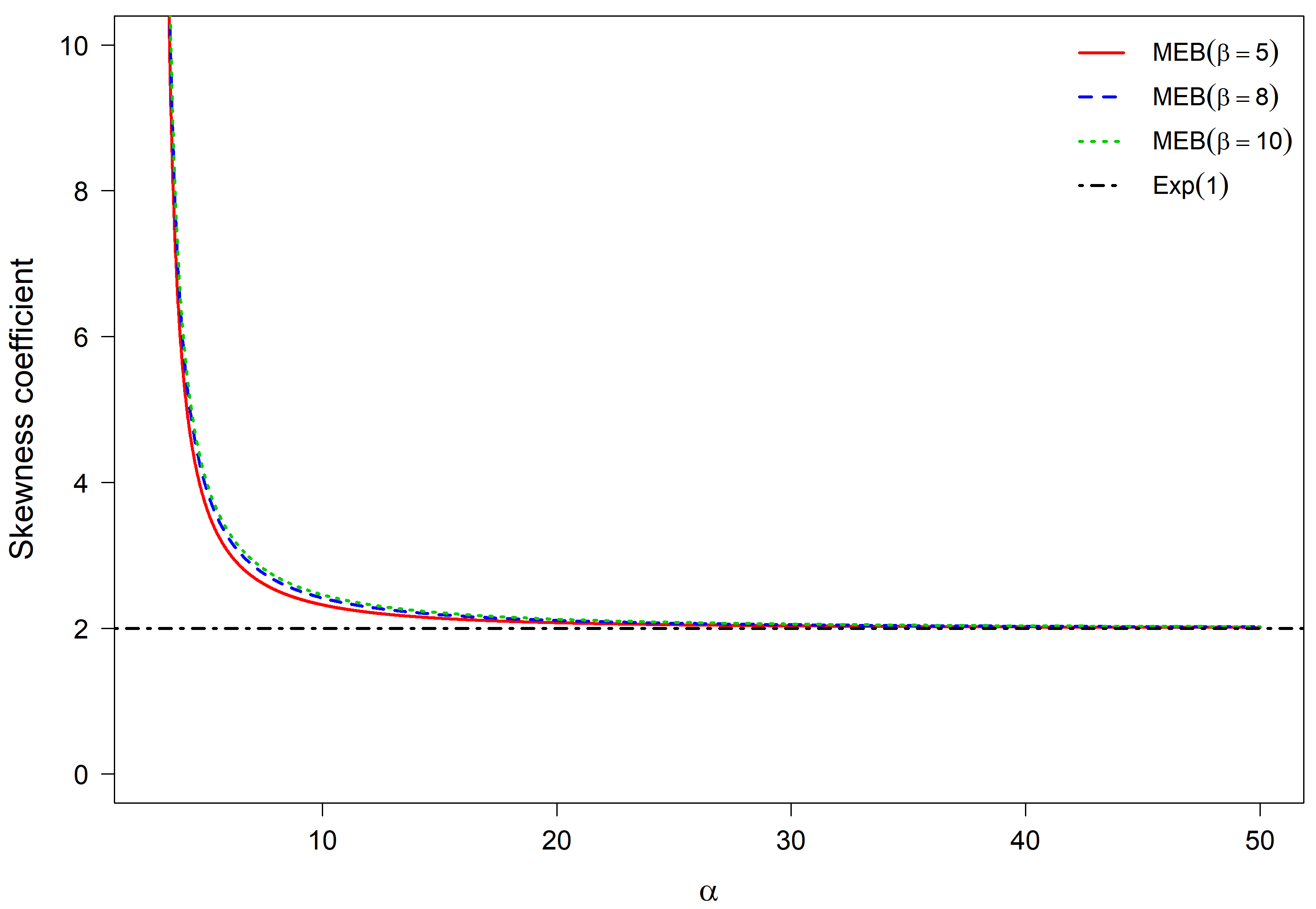
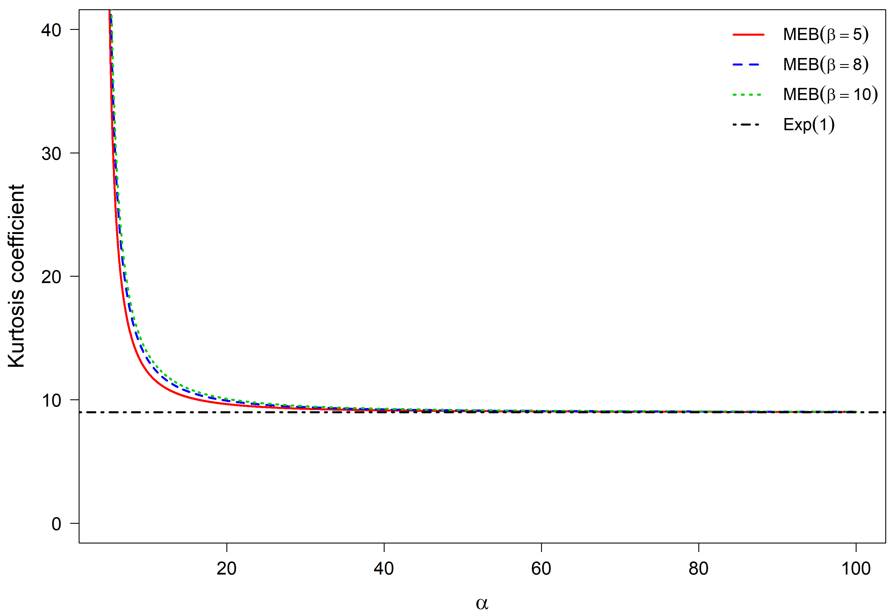
According to the moment existence conditions of the MEB distribution, the third-order moment exists when $\alpha >3$, while the fourth-order moment exists when $\alpha >4$. Therefore, the skewness and kurtosis coefficients are investigated to examine how the shape characteristics of the MEB distribution vary with the parameter $\alpha$. The corresponding results are presented in Figure 3 and Figure 4.

Figure 3. Comparison of skewness coefficient against $\alpha$ for the MEB distribution with different $\beta$ values and the Exp(1) distribution.

Figure 4. Comparison of kurtosis coefficient against $\alpha$ for the MEB distribution with different $\beta$ values and the Exp(1) distribution.

Figure 3 illustrates the effect of the shape parameters on the skewness coefficient of the MEB distribution. When $\alpha$ is close to the lower boundary for the existence of the third moment, the distribution presents a larger skewness coefficient and stronger right-skewed behavior. With increasing $\alpha$, the skewness coefficient decreases gradually and converges to 2, the value corresponding to the exponential distribution. The results demonstrate that the parameters $\alpha$ and $\beta$ provide effective control over the asymmetry of the MEB distribution, highlighting its flexibility in modeling asymmetric lifetime data.

Figure 4 shows the variation of the kurtosis coefficient of the MEB distribution with respect to $\alpha$ under different $\beta$ settings. For relatively small values of $\alpha$, the MEB distribution exhibits larger kurtosis coefficients than the Exp(1) distribution, indicating heavier tails and stronger extreme-value characteristics. As $\alpha$ increases, the kurtosis coefficient decreases gradually and approaches the value 9, which corresponds to the Pearson kurtosis of the exponential distribution with rate parameter 1.

The results demonstrate that the shape parameters $\alpha$ and $\beta$ provide effective control over the tail behavior and higher-order characteristics of the MEB distribution. Therefore, the proposed model offers greater flexibility than the exponential distribution for describing lifetime data with different tail properties.

3. Parameter Estimation

3.1. ML Estimation

Let $Z_1,Z_2,\cdots ,Z_n$ be a simple random sample of size n drawn from the population $Z\sim \mathrm{MEB}(\lambda ,\alpha ,\beta )$ and let $z_1,z_2,\cdots ,z_n$ denote the corresponding observations. The likelihood function is given by

$$l(\lambda ,\alpha ,\beta ;z_i)={\displaystyle \prod _{i=1}^n}2\lambda e^{-2\lambda z_i}{\displaystyle \frac{\alpha }{\alpha +\beta }}M(\beta ,\alpha +\beta +1;2\lambda z_i),$$

then the corresponding log-likelihood function is

$$L(\lambda ,\alpha ,\beta ;z_i)=n\log \left(2\lambda \right)-2\lambda {\displaystyle \sum _{i=1}^n}{z}_i+n\log \alpha -n\log (\alpha +\beta )+{\displaystyle \sum _{i=1}^n}\log M(\beta ,\alpha +\beta +1;2\lambda z_i).$$

(8)

Compute the first-order partial derivatives of Equation (8) with respect to $\lambda , \alpha$ and $\beta$, respectively, and set them to zero to yield the likelihood equations.

$${\displaystyle \frac{\partial L}{\partial \lambda }}={\displaystyle \frac{n}{\lambda }}-2{\displaystyle \sum _{i=1}^n}{z}_i+{\displaystyle \sum _{i=1}^n}{\displaystyle \frac{H_1(z_i;\lambda ,\alpha ,\beta )}{H(z_i;\lambda ,\alpha ,\beta )}}=0,$$

$${\displaystyle \frac{\partial L}{\partial \alpha }}={\displaystyle \frac{n}{\alpha }}-{\displaystyle \frac{n}{\alpha +\beta }}+{\displaystyle \sum _{i=1}^n}{\displaystyle \frac{H_2(z_i;\lambda ,\alpha ,\beta )}{H(z_i;\lambda ,\alpha ,\beta )}}=0,$$

$${\displaystyle \frac{\partial L}{\partial \beta }}=-{\displaystyle \frac{n}{\alpha +\beta }}+{\displaystyle \sum _{i=1}^n}{\displaystyle \frac{H_3(z_i;\lambda ,\alpha ,\beta )}{H(z_i;\lambda ,\alpha ,\beta )}}=0,$$

where $H(z_i;\lambda ,\alpha ,\beta )=M(\beta ,\alpha +\beta +1;2\lambda z_i)$, $H_1(z_i;\lambda ,\alpha ,\beta )={\displaystyle \frac{\partial H(z_i;\lambda ,\alpha ,\beta )}{\partial \lambda }}$, $H_2(z_i;\lambda ,\alpha ,\beta )={\displaystyle \frac{\partial H(z_i;\lambda ,\alpha ,\beta )}{\partial \alpha }}$, $H_3(z_i;\lambda ,\alpha ,\beta )={\displaystyle \frac{\partial H(z_i;\lambda ,\alpha ,\beta )}{\partial \beta }}$. The solutions $\widehat{\lambda }$, $\widehat{\alpha }$ and $\widehat{\beta }$ to the likelihood equations are the ML estimators of $\lambda$, $\alpha$ and $\beta$, respectively.

To establish the consistency of the ML estimator for the proposed MEB distribution, we first recall the following consistency result for likelihood equations.

Lemma 1

([16]). Suppose that $\ln p(x;\theta )$ is differentiable on Θ, and assume that $p(x;\theta )$ is identifiable, that is, for any $\theta \ne {\theta }^{\prime }$,

$$\{x:p(x;\theta )\ne p(x;{\theta }^{\prime })\}$$

is not a null set. Then the likelihood equation has a solution with probability one as $n\to \infty$, and this solution is consistent for θ.

Theorem 1.

For the MEB distribution with parameter vector $\mathit{\theta }=(\lambda ,\alpha ,\beta )$, where $\lambda >0$, $\alpha >0$, and $\beta >0$, the maximum likelihood estimator of θ obtained by the EM algorithm is consistent.

Proof. 

First, the log-density function of the MEB distribution is continuously differentiable with respect to the parameter vector $\mathit{\theta }=(\lambda ,\alpha ,\beta )$ on the parameter space $\mathsf{\Theta }$. Second, the MEB distribution is identifiable. Specifically, for any two different parameter vectors ${\mathit{\theta }}_1\ne {\mathit{\theta }}_2$, we have

$$\{z:f(z;{\mathit{\theta }}_1)\ne f(z;{\mathit{\theta }}_2)\}$$

is not a null set. Therefore, the MEB distribution satisfies the regularity conditions required for the consistency of maximum likelihood estimation. Accordingly, by Lemma 1, the maximum likelihood estimator obtained by the EM algorithm is consistent. □

3.2. EM Algorithm

Based on the stochastic representation of the MEB distribution given in Proposition 1, this paper adopts the iterative method of ML estimation based on the EM algorithm. To facilitate parameter inference, latent variables $X_1,X_2,\cdots ,X_n$ are introduced to simplify the estimation procedure.

$$Z_i|X_i=x\sim \mathrm{E}\left(2\lambda x\right),X_i\sim \mathrm{beta}(\alpha ,\beta ),$$

let $\theta =(\lambda ,\alpha ,\beta )$. The joint pdf of $(Z_i,X_i)$ is given by

$$f(z_i,x_i|\mathit{\theta })=f\left(z_i\right|x_i;\lambda )·f(x_i;\alpha ,\beta ),$$

where

$$\begin{array}{cc}\hfill f\left(z_i\right|x_i;\lambda )& =2\lambda x_i{e}^{-2\lambda x_i{z}_i},z_i>0,\hfill \\ \hfill f(x_i;\alpha ,\beta )& ={\displaystyle \frac{x_i^{\alpha -1}{(1-x_i)}^{\beta -1}}{B(\alpha ,\beta )}},0<x_i<1,\hfill \end{array}$$

then the log-likelihood function is

$${\mathcal{l}}_c(\mathit{\theta };z_i,x_i)=\log f\left(z_i\right|x_i;\lambda )+\log f(x_i;\alpha ,\beta ),$$

expanded as

$${\mathcal{l}}_c(\mathit{\theta };z_i,x_i)=\log \left(2\lambda x_i\right)-2\lambda x_i{z}_i+(\alpha -1)\log x_i+(\beta -1)\log (1-x_i)-\log B(\alpha ,\beta ),$$

for n independent random samples, the complete log-likelihood function is given by

$$L_c(\mathit{\theta };z_i,x_i)={\displaystyle \sum _{i=1}^n}\left[\log 2+\log \lambda +\alpha \log x_i-2\lambda x_i{z}_i+(\beta -1)\log (1-x_i)-\log B(\alpha ,\beta )\right].$$

E-step: Given the observed data $z_i$ and the current iterative parameter estimate ${\theta }^{\left(t\right)}$ compute the conditional expectation of the complete-data log-likelihood function with respect to the latent variable $X_i$, as follows

$$\begin{array}{cc}\hfill Q\left(\mathit{\theta }\right|{\mathit{\theta }}^{\left(t\right)})& ={\mathbb{E}}_{X_i|z_i,{\mathit{\theta }}^{\left(t\right)}}\left[L_c\left(\mathit{\theta }\right)\right].\hfill \end{array}$$

Let

$$\begin{array}{cc}\hfill A_i& =\mathbb{E}[\log X_i\mid z_i,{\mathit{\theta }}^{\left(t\right)}],\hfill \\ \hfill B_i& =\mathbb{E}[X_i\mid z_i,{\mathit{\theta }}^{\left(t\right)}],\hfill \\ \hfill C_i& =\mathbb{E}[\log (1-X_i)\mid z_i,{\mathit{\theta }}^{\left(t\right)}],\hfill \end{array}$$

the conditional expectation of the complete-data log-likelihood function with respect to the latent variables can be expressed as

$$Q(\mathit{\theta }\mid {\mathit{\theta }}^{\left(t\right)})={\displaystyle \sum _{i=1}^n}\left[\log 2+\log \lambda +\alpha A_i-2\lambda B_i{z}_i+(\beta -1)C_i-\log \mathrm{B}(\alpha ,\beta )\right].$$

(9)

M-step: Take the first-order partial derivatives of Equation (9) with respect to the parameters $\lambda ,\alpha ,$ and $\beta$ respectively, set all partial derivatives equal to zero, and solve the resulting system of likelihood equations to obtain the updated iterative values of $\lambda ,\alpha$ and $\beta$. Terms involving only $\lambda$,

$$Q_{\lambda }=n\log \lambda -2\lambda {\displaystyle \sum _{i=1}^n}{B}_i{z}_i,$$

differentiating with respect to the corresponding parameter yields

$$\begin{array}{cc}\hfill {\displaystyle \frac{\partial Q}{\partial \lambda }}& ={\displaystyle \frac{n}{\lambda }}-2{\displaystyle \sum _{i=1}^n}{B}_i{z}_i=0,\hfill \end{array}$$

solved by numerical methods

$$\begin{array}{cc}\hfill {\lambda }^{(t+1)}& ={\displaystyle \frac{n}{2{\displaystyle \sum _{i=1}^n}{B}_i{z}_i}}.\hfill \end{array}$$

Terms containing $\alpha$ and $\beta$

$$\begin{array}{cc}\hfill Q_{\alpha \beta }& =\alpha {\displaystyle \sum _{i=1}^n}{A}_i+\beta {\displaystyle \sum _{i=1}^n}{C}_i-{\displaystyle \sum _{i=1}^n}{C}_i-n\log \mathsf{\Gamma }\left(\alpha \right)-n\log \mathsf{\Gamma }\left(\beta \right)+n\log \mathsf{\Gamma }(\alpha +\beta ),\hfill \end{array}$$

let $\overline{A}={\displaystyle \frac{1}{n}}{\displaystyle \sum _{i=1}^n}{A}_i,\overline{C}={\displaystyle \frac{1}{n}}{\displaystyle \sum _{i=1}^n}{C}_i$, then

$$Q_{\alpha \beta }=n\left[\alpha \overline{A}+\beta \overline{C}-\overline{C}-\log \mathsf{\Gamma }\left(\alpha \right)-\log \mathsf{\Gamma }\left(\beta \right)+\log \mathsf{\Gamma }(\alpha +\beta )\right],$$

taking partial derivatives, we obtain

$$\begin{array}{cc}\hfill {\displaystyle \frac{\partial Q}{\partial \alpha }}& =n[\overline{A}-\psi \left(\alpha \right)+\psi (\alpha +\beta )]=0,\hfill \\ \hfill {\displaystyle \frac{\partial Q}{\partial \beta }}& =n[\overline{C}-\psi \left(\beta \right)+\psi (\alpha +\beta )]=0,\hfill \end{array}$$

where the function $\psi$ denotes the digamma function

$$\psi \left(x\right)={\displaystyle \frac{d}{dx}}\log \mathsf{\Gamma }\left(x\right),$$

thus, the iterative update equations of the parameters are obtained as follows

$$\begin{array}{cc}\hfill \psi \left({\alpha }^{(t+1)}\right)-\psi ({\alpha }^{(t+1)}+{\beta }^{(t+1)})& =\overline{A},\hfill \\ \hfill \psi \left({\beta }^{(t+1)}\right)-\psi ({\alpha }^{(t+1)}+{\beta }^{(t+1)})& =\overline{C},\hfill \end{array}$$

numerical methods are used to jointly solve the above equations for the updated estimates ${\alpha }^{(t+1)}$ and ${\beta }^{(t+1)}$.

Based on the current iterative parameter ${\mathit{\theta }}^{\left(t\right)}=({\lambda }^{\left(t\right)},{\alpha }^{\left(t\right)},{\beta }^{\left(t\right)})$, the corresponding posterior expectations are calculated with normalization.

$$f(x_i\mid z_i,{\mathit{\theta }}^{\left(t\right)})\propto f(z_i\mid x_i,{\lambda }^{\left(t\right)})f(x_i;{\alpha }^{\left(t\right)},{\beta }^{\left(t\right)}),$$

namely

$$f(x_i\mid z_i,{\mathit{\theta }}^{\left(t\right)})\propto \left(2{\lambda }^{\left(t\right)}{x}_i\right)e^{-2{\lambda }^{\left(t\right)}{x}_i{z}_i}{\displaystyle \frac{x_i^{{\alpha }^{\left(t\right)}-1}{(1-x_i)}^{{\beta }^{\left(t\right)}-1}}{B({\alpha }^{\left(t\right)},{\beta }^{\left(t\right)})}},$$

removing the constant factors independent of $x_i$, we obtain

$$f(x_i\mid z_i,{\mathit{\theta }}^{\left(t\right)})\propto x_i^{{\alpha }^{\left(t\right)}}{(1-x_i)}^{{\beta }^{\left(t\right)}-1}{e}^{-2{\lambda }^{\left(t\right)}{z}_i{x}_i},$$

conduct the normalization of posterior expectations

$$f(x_i\mid z_i,{\mathit{\theta }}^{\left(t\right)})={\displaystyle \frac{x^{{\alpha }^{\left(t\right)}}{(1-x)}^{{\beta }^{\left(t\right)}-1}{e}^{-c_{i}x}}{{\int }_0^1{t}^{{\alpha }^{\left(t\right)}}{(1-t)}^{{\beta }^{\left(t\right)}-1}{e}^{-c_{i}t}dt}},$$

where $c_i=2{\lambda }^{\left(t\right)}{z}_i$. Therefore, we get

$$\begin{array}{cc}\hfill A_i& ={\int }_0^1\log x·x^{{\alpha }^{\left(t\right)}}{(1-x)}^{{\beta }^{\left(t\right)}-1}{e}^{-c_{i}x}dx/K_i,\hfill \\ \hfill B_i& ={\int }_0^{1}x·x^{{\alpha }^{\left(t\right)}}{(1-x)}^{{\beta }^{\left(t\right)}-1}{e}^{-c_{i}x}dx/K_i,\hfill \\ \hfill C_i& ={\int }_0^1\log (1-x)x^{{\alpha }^{\left(t\right)}}{(1-x)}^{{\beta }^{\left(t\right)}-1}{e}^{-c_{i}x}dx/K_i,\hfill \end{array}$$

where $K_i={\int }_0^1{t}^{{\alpha }^{\left(t\right)}}{(1-t)}^{{\beta }^{\left(t\right)}-1}{e}^{-c_{i}t}dt$.

The E-step and M-step are repeated iteratively until the maximum difference between estimates from two consecutive iterations falls below a specified threshold, at which point the parameter estimates are finalized.

3.3. Observed Information Matrix

Let $Z_1,Z_2,\dots ,Z_n$ be a simple random sample of size n from the $\mathrm{MEB}(\lambda ,\alpha ,\beta )$ distribution. Let $\mathit{\theta }={(\lambda ,\alpha ,\beta )}^T$, and denote the log-likelihood function by $\mathcal{l}\left(\mathit{\theta }\right)$. The observed information matrix is defined as

$$I_n\left(\mathit{\theta }\right)=-{\nabla }^2\mathcal{l}\left(\mathit{\theta }\right)=-\left[\begin{array}{ccc}{\displaystyle \frac{{\partial }^2\mathcal{l}}{\partial {\lambda }^2}}& {\displaystyle \frac{{\partial }^2\mathcal{l}}{\partial \lambda \partial \alpha }}& {\displaystyle \frac{{\partial }^2\mathcal{l}}{\partial \lambda \partial \beta }}\\ {\displaystyle \frac{{\partial }^2\mathcal{l}}{\partial \alpha \partial \lambda }}& {\displaystyle \frac{{\partial }^2\mathcal{l}}{\partial {\alpha }^2}}& {\displaystyle \frac{{\partial }^2\mathcal{l}}{\partial \alpha \partial \beta }}\\ {\displaystyle \frac{{\partial }^2\mathcal{l}}{\partial \beta \partial \lambda }}& {\displaystyle \frac{{\partial }^2\mathcal{l}}{\partial \beta \partial \alpha }}& {\displaystyle \frac{{\partial }^2\mathcal{l}}{\partial {\beta }^2}}\end{array}\right].$$

In our implementation, the observed Hessian matrix is evaluated numerically at the ML estimate. To preserve positivity of the model parameters and improve numerical stability, the numerical differentiation is performed on the logarithmic parameterization

$$\mathit{\eta }={(\log \lambda ,\log \alpha ,\log \beta )}^T.$$

The Hessian matrix of the negative log-likelihood is symmetrized and checked for positive definiteness before inversion. Standard errors on the original parameter scale are subsequently obtained using the delta method.

When the estimated observed information matrix is nonsingular, the estimated covariance matrix of the maximum likelihood estimator is given by

$$\widehat{\mathrm{Var}}\left({\widehat{\mathit{\theta }}}_{\mathrm{ML}}\right)=I_n^{-1}\left({\widehat{\mathit{\theta }}}_{\mathrm{ML}}\right).$$

Accordingly, the approximate standard error of ${\widehat{\theta }}_j$ is

$$\mathrm{SE}\left({\widehat{\theta }}_j\right)=\sqrt{{\left[I_n^{-1}\left({\widehat{\mathit{\theta }}}_{\mathrm{ML}}\right)\right]}_{jj}},$$

and an approximate $100(1-\gamma )\%$ Wald confidence interval can be constructed as

$${\widehat{\theta }}_j\pm z_{1-\gamma /2}\mathrm{SE}\left({\widehat{\theta }}_j\right).$$

For a $95\%$ confidence interval, $z_{0.975}=1.96$.

3.4. Least-Squares Estimation

To provide an alternative to the EM-based ML estimation procedure, we also consider a LS estimator for the parameters of the MEB distribution. Let

$$Z_{\left(1\right)}\le Z_{\left(2\right)}\le \cdots \le Z_{\left(n\right)}$$

denote the ordered observations from a random sample of size n. The LS estimator is obtained by minimizing the squared differences between the fitted cumulative distribution function and the empirical plotting positions.

For the MEB distribution, the cumulative distribution function is

$$F_Z(z;\lambda ,\alpha ,\beta )=1-e^{-2\lambda z}M\left(\beta ,\alpha +\beta ;2\lambda z\right).$$

Therefore, define the least-squares objective function as

$$Q_{\mathrm{LS}}(\lambda ,\alpha ,\beta )={\displaystyle \sum _{i=1}^n}{\left[F_Z\left(Z_{\left(i\right)};\lambda ,\alpha ,\beta \right)-{\displaystyle \frac{i}{n+1}}\right]}^2.$$

(10)

Equivalently, using the explicit form of the MEB cumulative distribution function,

$$Q_{\mathrm{LS}}(\lambda ,\alpha ,\beta )={\displaystyle \sum _{i=1}^n}[1-e^{-2\lambda Z_{\left(i\right)}}M\left(\beta ,\alpha +\beta ;2\lambda Z_{\left(i\right)}\right)-{\displaystyle \frac{i}{n+1}}{]}^2.$$

The LS estimator is then defined by

$${\widehat{\mathit{\theta }}}_{\mathrm{LS}}={\left({\widehat{\lambda }}_{\mathrm{LS}},{\widehat{\alpha }}_{\mathrm{LS}},{\widehat{\beta }}_{\mathrm{LS}}\right)}^T=\underset{\lambda >0,\alpha >0,\beta >0}{\arg \min }{Q}_{\mathrm{LS}}(\lambda ,\alpha ,\beta ).$$

(11)

Since a closed-form solution of Equation (11) is not available, the minimization is carried out numerically. To preserve positivity of the three model parameters, the numerical optimization can be performed using the logarithmic parameterization

$$\mathit{\eta }={(\log \lambda ,\log \alpha ,\log \beta )}^T.$$

Unlike the EM-based maximum likelihood estimator, the LS estimator is constructed directly from the fitted cumulative distribution function and does not rely on the latent-variable representation of the MEB model. It therefore provides a complementary estimation procedure for assessing the finite-sample performance of parameter estimation.

3.5. Computational Efficiency and Convergence Diagnostics of the EM Algorithm

In the numerical implementation of the EM algorithm, the E-step involves integrals that are approximated using a 128-point Gauss–Legendre quadrature rule to ensure sufficient accuracy. The update of the scale parameter $\lambda$ is obtained in closed form, while the shape parameters $\alpha$ and $\beta$ are updated jointly by solving the digamma equations using Newton–Raphson iterations with step halving to enhance numerical stability. The outer EM iterations are terminated when the maximum relative change of the updated parameter vector $(\lambda ,\alpha ,\beta )$ falls below ${10}^{-5}$, with a maximum of 5000 iterations allowed to prevent infinite loops. These settings are consistently applied throughout the simulation study and real-data analyses.

The EM algorithm provides an effective approach for obtaining the maximum likelihood estimates of the MEB distribution. However, compared with direct optimization methods, the EM algorithm may require additional computational effort due to its iterative nature. To evaluate the computational efficiency and numerical stability of the proposed estimation procedure, a simulation study was conducted to investigate the convergence behavior, average number of iterations, and computational time of the EM algorithm.

For each sample size, multiple independent replications were performed under the same parameter setting. The convergence criterion was based on the relative change of the log-likelihood value between two consecutive iterations. The average number of iterations and the average CPU time were recorded to assess the computational burden of the proposed EM procedure. The results are summarized in Table 2.

Table 2. Computational performance of the EM algorithm under different sample sizes.

Sample Size	Average Iterations	Median Iterations	Average CPU Time (s)
100	1224.47	655.50	20.99
300	1439.10	985.00	49.11
500	1454.88	1047.00	74.64

Table 2 shows that the proposed EM algorithm has similar convergence patterns under different sample sizes. As expected, the computational time increases with the sample size because the evaluation of the likelihood-related quantities involves more observations. Nevertheless, the average number of iterations remains within a relatively narrow range, indicating that the convergence speed of the EM algorithm is not substantially affected by the sample size. Although the proposed MEB model requires more computational effort than simpler exponential-type models due to the latent variable representation and additional shape parameters, the computational cost remains acceptable for practical applications.

To investigate the influence of initial parameter selection on the EM algorithm, three sets of starting values were considered by multiplying the initial parameter vector by factors 0.9, 1.0, and 1.1. The convergence behavior under different initial values is summarized in Table 3. The reported average iterations are calculated only from replications that reached valid converged solutions.

Table 3. Effect of initial values on the convergence behavior of the EM algorithm.

n	Initial Value	Convergence Rate	Valid Solution Rate	Mean Iterations
100	0.9	0.410	0.262	1126.17
100	1.0	0.408	0.256	1168.38
100	1.1	0.417	0.257	1246.90
300	0.9	0.423	0.416	1277.07
300	1.0	0.424	0.415	1426.89
300	1.1	0.422	0.413	1497.76
500	0.9	0.438	0.438	1238.34
500	1.0	0.435	0.435	1409.55
500	1.1	0.435	0.435	1602.02

The results in Table 3 indicate that moderate changes in the initial values have limited influence on the convergence performance of the EM algorithm. The convergence rates and valid solution rates are very similar among different starting values. Moreover, the average number of iterations required for valid converged solutions remains within a comparable range, suggesting that the proposed EM algorithm is reasonably robust to the choice of initial values. Therefore, the estimation results are not sensitive to moderate perturbations of the starting parameter values.

3.6. Numerical Simulation

To evaluate the finite-sample performance of the parameter estimators of the MEB distribution under different distributional settings, a Monte Carlo simulation study is conducted. Three parameter configurations and sample sizes $n=100$, 300, and 500 are considered. For each combination of parameter setting and sample size, random samples are generated from the corresponding MEB distribution, and the simulation experiment is independently repeated 1000 times.

Two estimation procedures are considered. The first is the EM-based maximum likelihood estimator developed in this work. The second is the LS estimator. For a fair comparison, both estimators are evaluated under the same parameter settings and sample sizes.

The finite-sample performance is assessed in terms of empirical bias, relative bias, standard error (SE), root mean square error (RMSE), and coverage probability (CP). For each estimation procedure, these summaries are calculated from the retained valid replications satisfying the corresponding numerical convergence and screening criteria. The results are reported in Table 4.

Table 4. Monte Carlo comparison of the EM-based maximum likelihood and LS estimators of the MEB distribution.

n	$(\mathit{\lambda },\mathit{\alpha },\mathit{\beta })$	Parameter	EM-Based ML					LS
			Bias	Relative Bias	SE	RMSE	CP	Bias	Relative Bias	SE	RMSE	CP
100	$(1,3,1.2)$	$\lambda$	0.0315	0.1412	0.1791	0.1816	0.9542	0.2703	0.2703	0.8822	0.9214	0.9551
		$\alpha$	0.1312	0.2629	0.9824	0.9900	0.9346	−0.5800	−0.1933	0.9199	1.0862	0.9551
		$\beta$	−0.0022	0.0564	0.0858	0.0857	0.9412	0.2464	0.2053	2.0446	2.0561	0.9487
	$(1.1,3.5,1.2)$	$\lambda$	0.0659	0.0600	0.1873	0.1983	0.9066	0.3751	0.3410	0.9726	1.0408	0.9370
		$\alpha$	−0.1425	−0.0407	0.8932	0.9034	0.9730	−0.7807	−0.2231	1.1302	1.3719	0.9556
		$\beta$	0.0126	0.0105	0.0713	0.0723	0.9287	0.3926	0.3272	2.4487	2.4755	0.9370
	$(1.2,3.2,1.2)$	$\lambda$	0.0698	0.0582	0.2157	0.2265	0.9336	0.3160	0.2634	0.9901	1.0379	0.9399
		$\alpha$	−0.0375	−0.0117	0.8810	0.8807	0.9597	−0.6834	−0.2136	1.0248	1.2304	0.9715
		$\beta$	0.0060	0.0050	0.1142	0.1142	0.9929	0.2661	0.2218	2.3556	2.3669	0.9557
300	$(1,3,1.2)$	$\lambda$	0.0047	0.0870	0.1089	0.1089	0.9522	0.1001	0.1001	0.5927	0.6004	0.9497
		$\alpha$	0.1449	0.1787	0.6655	0.6807	0.9328	0.0581	0.0194	1.0830	1.0832	0.9418
		$\beta$	0.0069	0.0396	0.0622	0.0626	0.9341	0.2970	0.2475	2.3170	2.3329	0.9497
	$(1.1,3.5,1.2)$	$\lambda$	0.0311	0.0283	0.1205	0.1244	0.9335	0.1219	0.1109	0.5455	0.5582	0.9463
		$\alpha$	−0.0208	−0.0059	0.7508	0.7505	0.9552	−0.2426	−0.0693	1.1197	1.1440	0.9612
		$\beta$	0.0118	0.0098	0.0521	0.0534	0.9422	0.2325	0.1937	2.1818	2.1909	0.9612
	$(1.2,3.2,1.2)$	$\lambda$	0.0160	0.0133	0.1293	0.1302	0.9407	0.1720	0.1433	0.6798	0.7003	0.9351
		$\alpha$	0.0989	0.0309	0.6921	0.6986	0.9352	0.0374	0.0117	1.2033	1.2023	0.9429
		$\beta$	0.0093	0.0078	0.0580	0.0587	0.9434	0.5680	0.4733	2.7186	2.7738	0.9403
500	$(1,3,1.2)$	$\lambda$	−0.0041	0.0742	0.0928	0.0929	0.9582	0.0384	0.0384	0.4468	0.4479	0.9538
		$\alpha$	0.1883	0.1641	0.6139	0.6418	0.9233	0.2268	0.0756	1.1026	1.1245	0.9253
		$\beta$	0.0074	0.0317	0.0493	0.0498	0.9408	0.2715	0.2263	2.3257	2.3390	0.9516
	$(1.1,3.5,1.2)$	$\lambda$	0.0118	0.0107	0.0984	0.0990	0.9437	0.0951	0.0864	0.5049	0.5132	0.9474
		$\alpha$	0.1177	0.0336	0.7498	0.7585	0.9334	0.0487	0.0139	1.1063	1.1060	0.9474
		$\beta$	0.0113	0.0094	0.0388	0.0404	0.9360	0.3482	0.2902	2.3831	2.4055	0.9524
	$(1.2,3.2,1.2)$	$\lambda$	0.0019	0.0016	0.1014	0.1014	0.9509	0.0796	0.0663	0.5476	0.5527	0.9593
		$\alpha$	0.1489	0.0465	0.6466	0.6632	0.9324	0.1517	0.0474	1.2296	1.2375	0.9276
		$\beta$	0.0083	0.0069	0.0458	0.0465	0.9435	0.3170	0.2642	2.4315	2.4494	0.9525

The results in Table 4 show that the estimation accuracy of the proposed EM-based maximum likelihood estimator improves as the sample size increases. The SE and RMSE values generally decrease with increasing sample size, while the biases remain small and the coverage probabilities are close to the nominal level of $0.95$, indicating satisfactory finite-sample performance.

Compared with the LS estimator, the EM-based estimator generally achieves smaller SE and RMSE values, especially for the parameter $\beta$. Although the LS estimator provides reasonable interval coverage, it exhibits larger estimation variability. These results demonstrate the effectiveness and stability of the proposed EM-based estimation procedure.

On this basis, a model-comparison simulation is conducted to evaluate the fitting performance of the proposed MEB distribution against several competing models, including SME, WE, Exp, Weibull, and GE distributions. The SME model is considered as a direct competitor since it is a special case of the MEB family when $\alpha =\beta =q$.

Samples are generated from the MEB distribution with $n=100$, 300, and 500, using 500 independent replications for each setting. The fitted models are compared using the maximized log-likelihood, Akaike information criterion (AIC), Anderson–Darling (AD) statistic, and bootstrap p-value. The corresponding results are summarized in Table 5.

Table 5. Average fitting results for MEB-generated samples.

n	Model	Log-Likelihood	AIC	AD	p-Value
100	MEB	−53.7644	113.5288	0.4795	0.7849
	SME	−52.9217	111.8434	0.4880	0.7735
	WE	−55.2959	114.5918	0.9752	0.5350
	Exp	−55.6129	113.2259	0.9518	0.5379
	Weibull	−56.2995	116.5989	1.5532	0.5699
	GE	−54.7807	113.5614	0.5468	0.7398
300	MEB	−163.6019	333.2039	0.4474	0.8033
	SME	−163.8533	331.7066	0.4923	0.7701
	WE	−168.7405	341.4811	1.5625	0.3610
	Exp	−169.0151	340.0303	1.5288	0.3704
	Weibull	−174.3650	352.7299	5.5024	0.3323
	GE	−167.5561	339.1121	0.8363	0.5842
500	MEB	−271.3220	548.6440	0.4449	0.8047
	SME	−271.5907	547.1814	0.4916	0.7666
	WE	−278.1816	560.3632	1.9458	0.2636
	Exp	−278.5041	559.0081	1.8991	0.2745
	Weibull	−284.9910	573.9820	6.6328	0.2175
	GE	−276.6037	557.2073	0.9809	0.5022

The results in Table 5 show that the proposed MEB distribution provides competitive fitting performance for data generated from the MEB model. Across different sample sizes, the MEB model achieves log-likelihood values comparable to the best-fitting models and consistently smaller AD statistics than most of the competing models, indicating its ability to recover the underlying distributional characteristics.

Compared with the SME distribution, the MEB model provides additional flexibility through the asymmetric beta mixing mechanism with two separate shape parameters. While SME obtains slightly smaller AIC values across all sample sizes due to its lower model complexity, the MEB model achieves improvements in log-likelihood and AD statistics, reflecting its superior fitting capability.

Overall, the simulation results confirm that the proposed MEB distribution can effectively capture the characteristics of the generated data and provides a more flexible scale-mixture framework than the competing models. All numerical computations were performed in R (version 4.5.2).

4. Application

In this section, we further investigate the practical applicability of the proposed MEB distribution using an actual dataset. The fitting performance of the proposed model is compared with several commonly used lifetime distributions, including the Exp, SME, WE, Weibull, and GE distributions. The comparison is conducted based on several goodness-of-fit criteria to evaluate the flexibility and effectiveness of the proposed model in describing real data. The pdfs of the competing distributions are given as follows.

$$f(x;\lambda )=\left\{\begin{array}{cc}\lambda e^{-\lambda x}\hfill & x\ge 0,\hfill \\ 0\hfill & x<0,\hfill \end{array}\right.$$

$$f(x;\lambda ,q)=\lambda e^{-\lambda x}M\left(q,2q+1;2\lambda x\right),x>0,\lambda ,q>0,$$

$$f(x;\alpha ,\lambda )={\displaystyle \frac{\alpha +1}{\alpha }}\lambda e^{-\lambda x}\left(1-e^{-\alpha \lambda x}\right),x>0,\lambda ,\alpha >0,$$

$$f(x;k,\theta )={\displaystyle \frac{k}{\theta }}{\left({\displaystyle \frac{x}{\theta }}\right)}^{k-1}\exp \left[-{\left({\displaystyle \frac{x}{\theta }}\right)}^k\right],x>0,$$

$$f(x;\alpha ,\lambda )=\alpha \lambda e^{-\lambda x}{\left(1-e^{-\lambda x}\right)}^{\alpha -1},x>0.$$

4.1. Application to Airborne Communication Receiver Data

This dataset contains the maintenance time (hours) of 46 airborne communication receivers, as reported by Devore [17]. The data are listed in Table 6.

Table 6. Sample data of maintenance duration (hours) for 46 airborne communication receivers.

0.2	0.3	0.5	0.5	0.5	0.6	0.6	0.7	0.7	0.7
0.8	0.8	0.8	1.0	1.0	1.0	1.0	1.1	1.3	1.5
1.5	1.5	1.5	2.0	2.0	2.2	2.5	2.7	3.0	3.0
3.3	3.3	4.0	4.0	4.5	4.7	5.0	5.4	5.4	7.0
7.5	8.8	9.0	10.3	22.0	24.5

To further evaluate the practical applicability of the proposed MEB distribution, an actual dataset is analyzed and compared with several competing distributions, including the SME, WE, Exp, Weibull, and GE distributions. Table 7 presents the maximum log-likelihood estimates of the model parameters together with several goodness-of-fit criteria, including the log-likelihood, AIC, AD statistic, and p-value.

Table 7. Comparison of parameter estimation and model fitting performance.

Parameters	MEB	SME	WE	Exp	Weibull	GE
$\widehat{\lambda }$	0.3945	0.3700	0.2908	0.2768	3.4100	0.2715
$\widehat{\alpha }$	2.4140	—	18.7573	—	—	0.9720
$\widehat{\beta }$	2.7191	—	—	—	—	—
$\widehat{q}$	—	2.3357	—	—	—	—
$\widehat{k}$	—	—	—	—	0.9039	—
log-likelihood	−103.0498	−103.0502	−103.7899	−105.0893	−104.6099	−105.0791
AIC	212.0996	210.1004	211.5799	212.1786	213.2197	214.1581
AD	0.6330	0.6306	1.5921	1.2687	0.9296	1.2116
p-value	0.4871	0.4906	0.0983	0.1883	0.5082	0.2186

The results in Table 7 show that different criteria provide complementary perspectives on model performance. The proposed MEB distribution achieves the largest log-likelihood value among all considered models, indicating its superior likelihood-based fitting performance and greater modeling flexibility. Meanwhile, the SME model, as a restricted special case of the MEB family, obtains the smallest AD statistic and the smallest AIC value due to its simpler parameterization.

Compared with the traditional competing distributions, including the WE, Exp, Weibull, and GE models, both the MEB and SME distributions provide competitive fitting performance according to the likelihood-based and goodness-of-fit criteria. These results indicate that the general beta mixing mechanism introduced in the MEB distribution improves the flexibility of the model, while the SME model remains an effective simplified alternative when a more parsimonious structure is preferred.

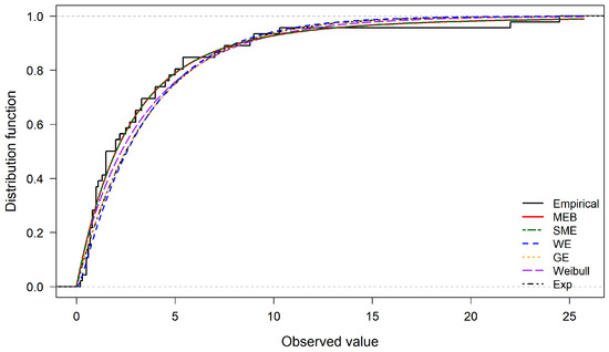
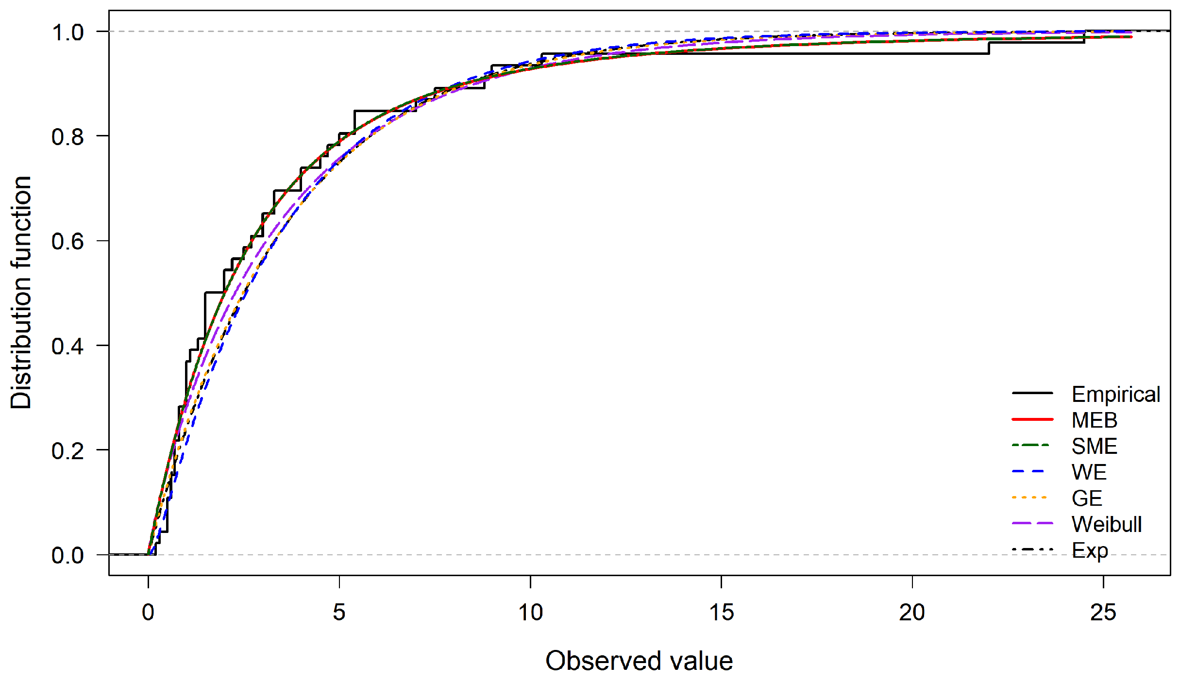
To further illustrate the fitting performance of the considered distributions, Figure 5 presents the empirical distribution function together with the fitted cdfs.

Figure 5. Empirical distribution function and fitted cdfs for the maintenance time data.

The results show that the fitted cumulative distribution functions of the considered models provide reasonable agreement with the empirical distribution over the observed range. Among these models, the proposed MEB distribution exhibits a close fit to the empirical distribution and provides greater flexibility due to its general beta mixing mechanism. The SME distribution, as a simpler special case of the MEB family, also shows competitive fitting performance. Overall, the comparison indicates that the proposed MEB distribution is capable of effectively describing the distributional characteristics of the maintenance time data.

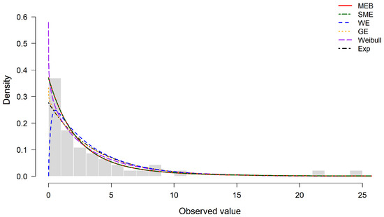
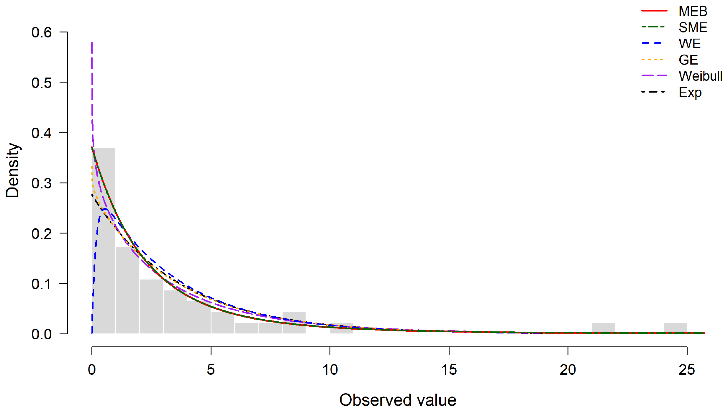
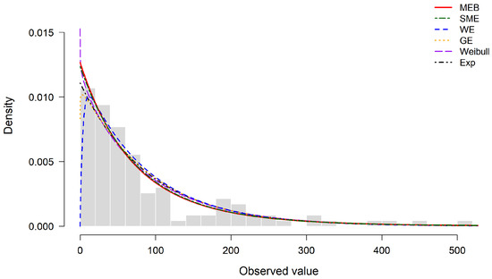
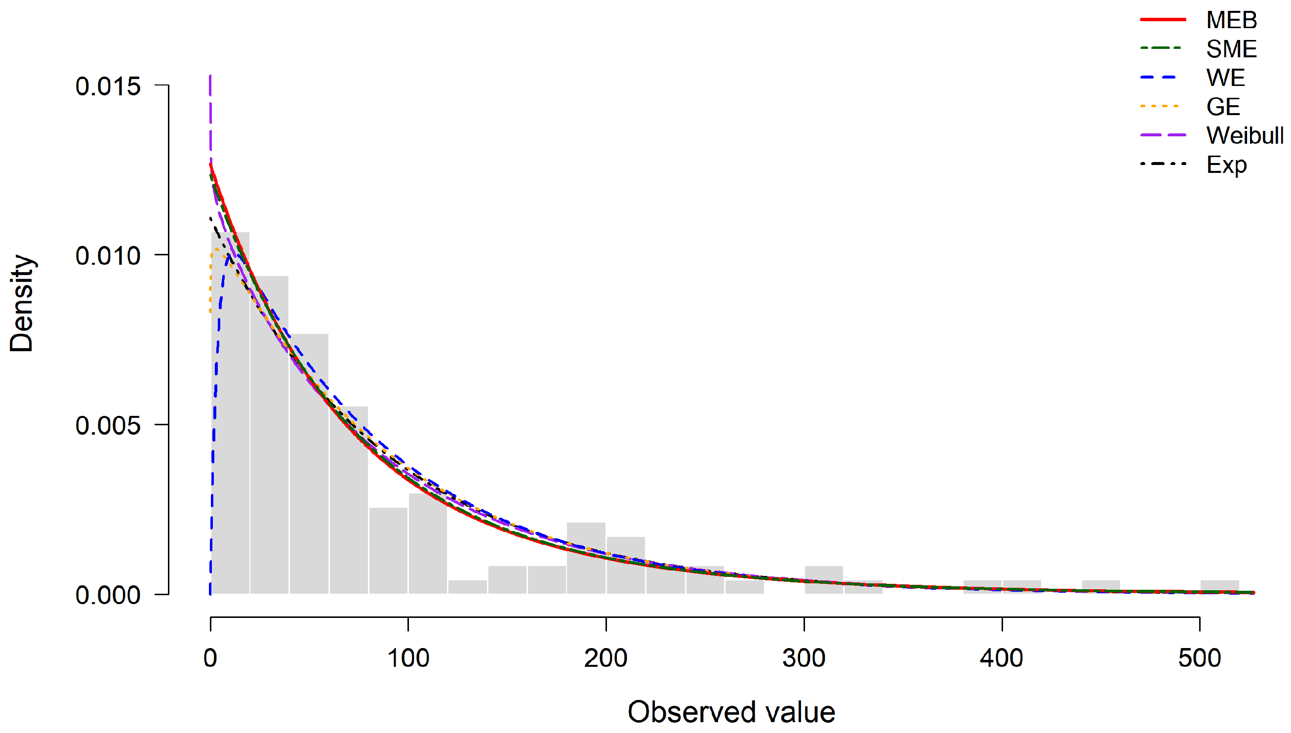
To further evaluate the fitting performance of the proposed MEB distribution, the fitted pdfs of MEB and other competing distributions are compared with the histogram of the maintenance time data.

Figure 6 shows that all considered models are able to capture the right-skewed pattern of the maintenance time data. The proposed MEB distribution provides a flexible representation of the empirical density over the main observation range and gives a competitive fit in the tail region. The SME distribution, as a simpler special case of the MEB family, also provides a comparable approximation with fewer parameters. Overall, the fitted density curves indicate that the proposed scale-mixture framework is effective for describing the skewed characteristics of the maintenance time data.

Figure 6. Comparison between the histogram of the maintenance time data and the fitted pdfs of the considered distributions.

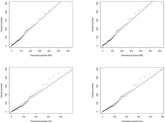
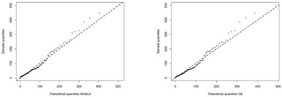
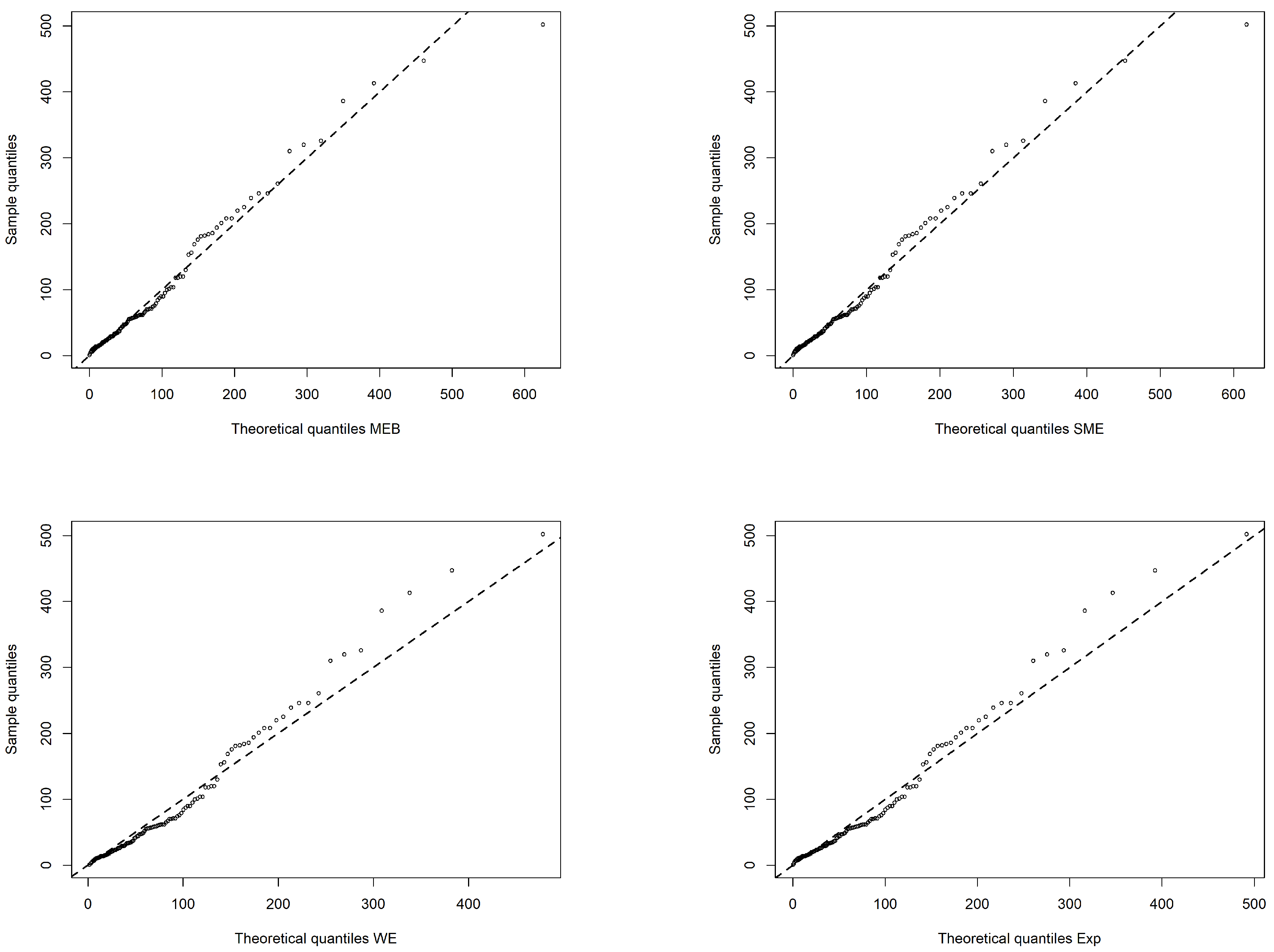
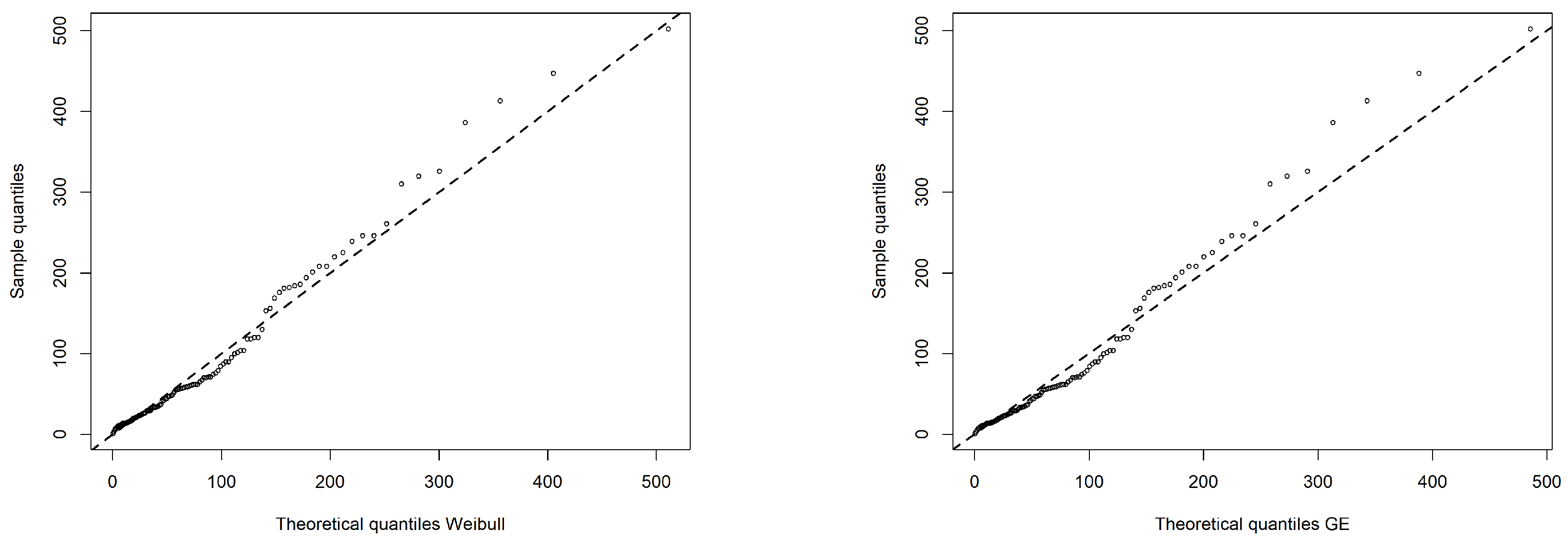
To further assess the fitting behavior of the considered distributions, Q-Q plots are provided in Figure 7.

Figure 7. Q-Q plots of the fitted distributions for the repair-time data of 46 airborne communication receivers.

The Q-Q plots in Figure 7 show that the MEB distribution (which nests the SME distribution as a special case) yields the closest overall agreement between the fitted theoretical quantiles and the observed sample quantiles. Most points lie near the reference line, though a noticeable deviation persists for one of the largest observations. The Weibull distribution also provides a reasonable fit, particularly in the upper tail. In contrast, the exponential, weighted exponential, and generalized exponential distributions exhibit more pronounced departures from the line for the largest observations. Overall, these Q-Q plots corroborate the earlier goodness-of-fit results, supporting the conclusion that the MEB distribution offers a comparatively better description of the repair-time data, especially in terms of tail behavior.

4.2. Application to the Inter-Failure Times of the Air Conditioning Systems of Boeing 720 Jet Aircraft

This dataset consists of the inter-failure times (hours) of the air conditioning systems of individual Boeing 720 jet aircraft in a fleet, as reported by Proschan [18]. In this study, the observations from six aircraft numbered 7907, 7908, 7909, 7910, 7911, and 7912 are selected for analysis. The selected failure interval data are listed in Table 8.

Table 8. Failure intervals (hours) of the air conditioning systems of six Boeing 720 aircraft (Nos.7907–7912).

194	15	41	29	33	181	413	14	58	37	100	65	9	169	447
184	36	201	118	34	31	18	18	67	57	62	7	22	34	90
10	60	186	61	49	14	24	56	20	79	84	44	59	29	118
25	156	310	76	26	44	23	62	130	208	70	101	208	74	57
48	29	502	12	70	21	29	386	59	27	153	26	326	55	320
56	104	220	239	47	246	176	182	33	15	104	35	23	261	87
7	120	14	62	47	225	71	246	21	42	20	5	12	120	11
3	14	71	11	14	11	16	90	1	16	52	95

Following the analysis in Section 4.1, the proposed MEB distribution is applied to this dataset and compared with several competing distributions, including SME, WE, Exp, Weibull, and GE. Table 9 presents the maximum likelihood estimates of the model parameters and several goodness-of-fit criteria.

Table 9. Comparison of parameter estimation and model fitting performance.

Parameters	MEB	SME	WE	Exp	Weibull	GE
$\widehat{\lambda }$	0.0922	0.0124	0.0115	0.0111	—	0.0113
$\widehat{\alpha }$	7.3752	—	23.4714	—	—	1.0294
$\widehat{\beta }$	100.0000	—	—	—	—	—
$\widehat{q}$	—	5.2639	—	—	—	—
$\widehat{k}$	—	—	—	—	0.9705	—
$\widehat{\theta }$	—	—	—	—	88.9243	—
log-likelihood	−643.0066	−643.1244	−642.2348	−643.7552	−643.6613	−643.7279
AIC	1292.0131	1290.2488	1288.4696	1289.5104	1291.3226	1291.4558
AD	0.8181	0.8408	1.5083	1.2561	1.1048	1.3403
p-value	0.6296	0.5963	0.1872	0.2288	0.3164	0.2020

Table 9 shows that the proposed MEB distribution provides competitive performance for the Boeing 720 aircraft failure interval data. Although the WE distribution achieves the largest log-likelihood and the smallest AIC value, the proposed MEB distribution obtains the smallest AD statistic and the largest p-value among all competing models. This indicates that the MEB distribution provides a better overall fit, particularly in capturing the distributional characteristics and tail behavior of the failure interval data.

To further evaluate the fitting capability of the proposed MEB distribution, the fitted density curves of the MEB distribution and several competing distributions are compared with the histogram of the Boeing 720 aircraft failure interval data.

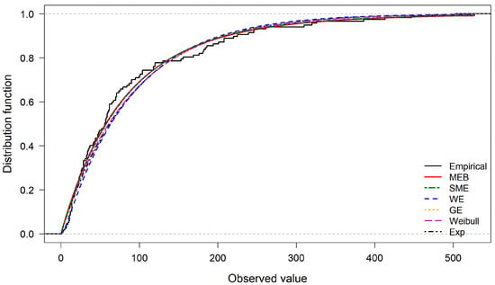
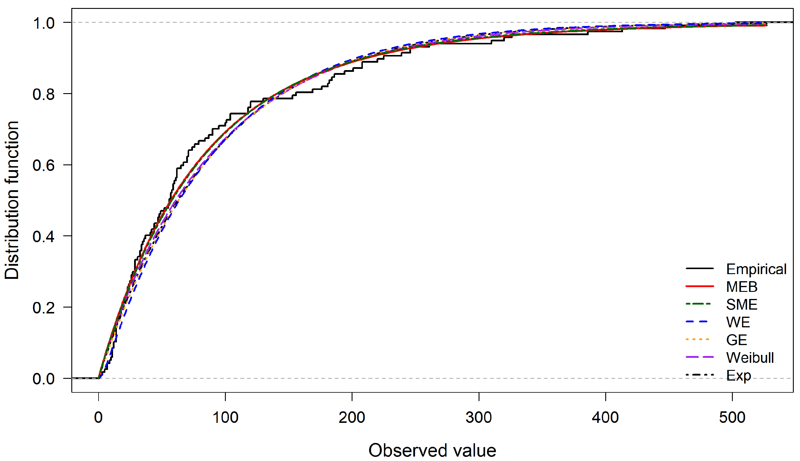
Figure 8 compares the empirical distribution function of the Boeing 720 aircraft failure interval data with the fitted distribution functions of the MEB distribution and several competing models. It can be observed that the proposed MEB distribution provides a close fit to the empirical distribution over the entire range of observations. In particular, the MEB model captures the distributional behavior and tail characteristics of the failure interval data more effectively than the conventional exponential-type models. These graphical results are consistent with the goodness-of-fit measures reported in Table 9.

Figure 8. Comparison of empirical and fitted distribution functions for Boeing 720 aircraft failure interval data.

Figure 9 illustrates the fitted density curves of the proposed MEB distribution and several competing distributions for the Boeing 720 aircraft failure interval data. The histogram represents the empirical distribution of the observed failure intervals, while the curves correspond to the fitted probability density functions obtained by different models. It can be observed that the proposed MEB distribution provides a close fit to the empirical data over the entire range of observations. In particular, the MEB density curve captures the decreasing trend and the long-tail behavior of the failure interval data effectively. Compared with the other competing distributions, the MEB distribution shows a more flexible fitting ability, especially in describing the tail region of the data.

Figure 9. Comparison of fitted density curves for Boeing 720 aircraft failure interval data.

To further assess the fitting behavior of the considered distributions, Q-Q plots are provided in Figure 10.

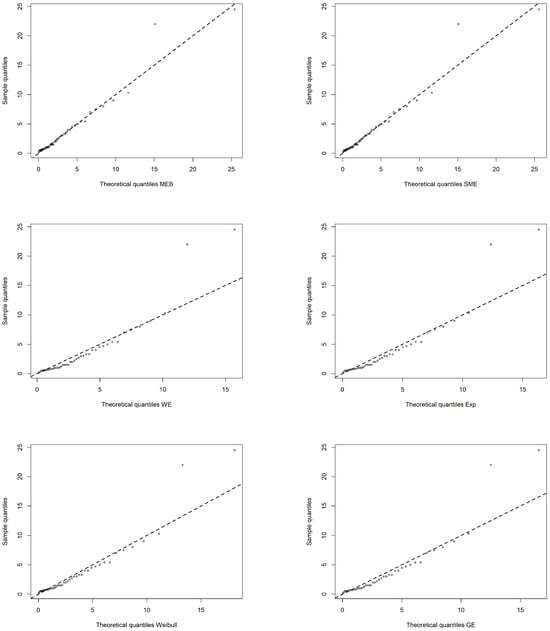
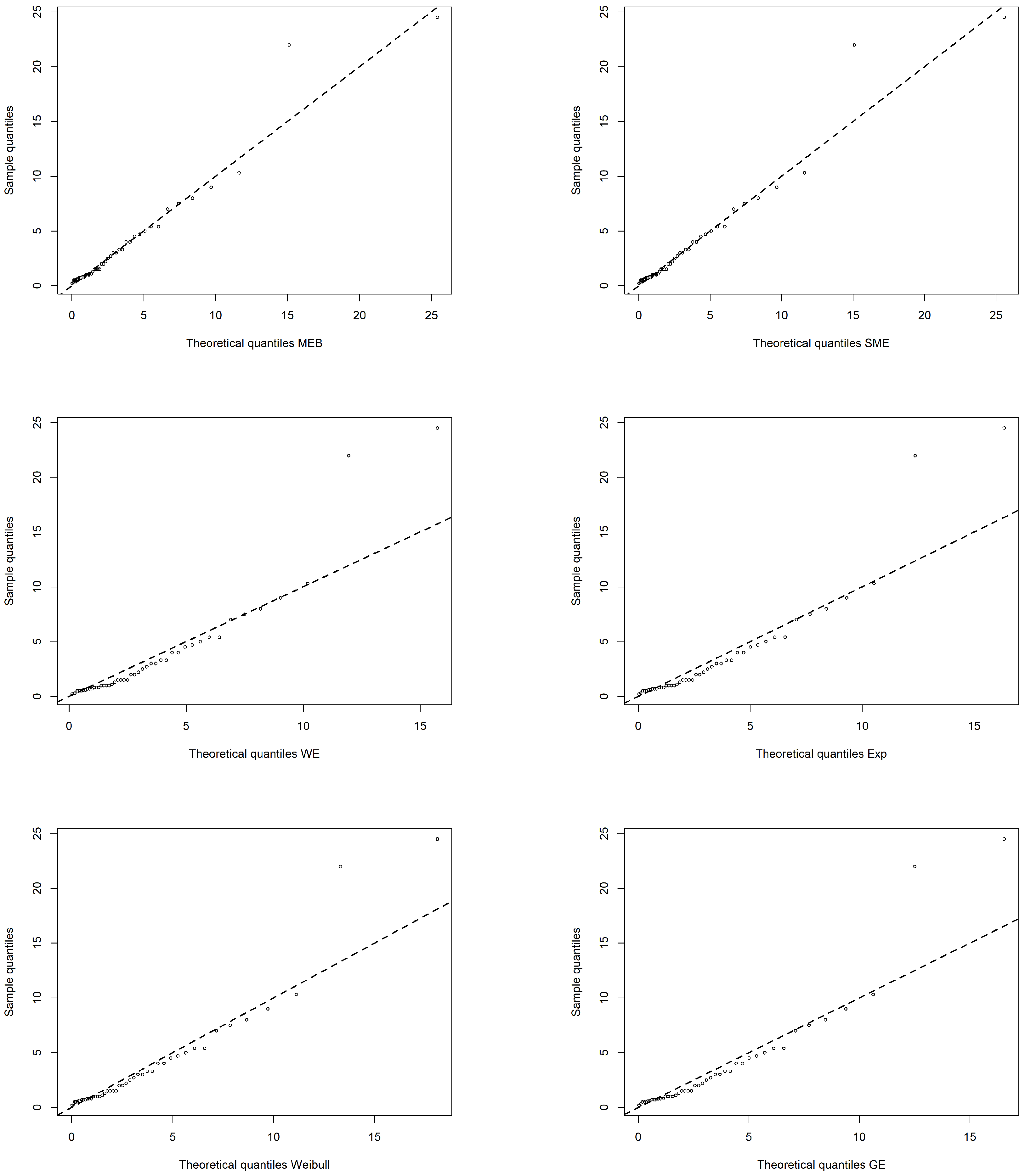
Figure 10. Q-Q plots of the fitted distributions for the Boeing 720 aircraft failure interval data.

The Q-Q plots of the fitted distributions are presented in Figure 10. It can be observed that the proposed MEB distribution provides a good agreement between the theoretical and empirical quantiles, especially in the tail region. The SME distribution also shows a comparable performance, while the other competing models exhibit larger deviations. These results further demonstrate the superiority of the MEB distribution in fitting the failure interval data.

5. Conclusions

In this paper, we proposed a new extended exponential distribution, called the MEB distribution, based on a scale-mixture representation involving exponential and beta distributions. The proposed model extends the classical exponential distribution by introducing two additional shape parameters, which provide greater flexibility in describing asymmetric lifetime data and observations with different tail characteristics.

The main statistical properties of the MEB distribution were systematically investigated, including its pdf, cdf, reliability function, moments, skewness, and kurtosis. In addition, the limiting relationship between the proposed model and the exponential distribution was established, showing that the exponential distribution can be obtained as a special limiting case under appropriate parameter conditions.

For parameter estimation, a ML estimation procedure based on the EM algorithm was developed by utilizing the stochastic representation of the MEB distribution. The proposed EM algorithm provides an effective approach for estimating the model parameters. Furthermore, the performance of the EM-based maximum likelihood estimator was compared with that of the least-squares estimation method through Monte Carlo simulations. The numerical results demonstrate that the EM-based ML estimator generally provides more accurate and stable parameter estimates, indicating its advantage for statistical inference of the proposed MEB distribution.

The practical applicability of the proposed model was further illustrated through two real data analyses. Compared with several existing exponential-type distributions, the MEB distribution showed competitive fitting performance and greater flexibility in capturing the skewness and tail behavior of positive lifetime data.

Although the present study focuses on parameter estimation based on the EM algorithm, further investigations are still needed. In particular, the theoretical development and computational implementation of interval estimation for the MEB distribution, including the construction of confidence intervals and related estimation algorithms, will be considered in future research.

References

- Andrews, D.F.; Mallows, C.L. Scale mixtures of normal distributions. J. R. Stat. Soc. Ser. B 1974, 36, 99–102. [Google Scholar] [CrossRef] [Scilit]
- Choy, S.T.B.; Chan, J.S.K.; Makov, U.E. Robust Bayesian analysis of loss reserving data using scale mixtures distributions. J. Appl. Stat. 2016, 43, 396–411. [Google Scholar] [CrossRef] [Scilit]
- Zhou, X.D.; Chen, S.Y. Analysis of test scores based on scale mixture of skew-normal distributions. Stat. Appl. 2024, 13, 1677–1689. [Google Scholar] [CrossRef]
- Kim, H.M. A note on scale mixtures of skew normal distribution. Stat. Probab. Lett. 2008, 78, 1694–1701. [Google Scholar] [CrossRef] [Scilit]
- Xia, Y.M.; Liu, Y.A. Robust Bayesian analysis of general factor analysis model based on normal scale mixture. Appl. Probab. Stat. 2014, 30, 423–438. [Google Scholar] [CrossRef]
- Haq, M.A.; Hashmi, S.; Aslam, M. Marshall–Olkin length biased exponential distribution for wind speed analysis alternative to Weibull distribution. Model. Earth Syst. Environ. 2024, 10, 1095–1108. [Google Scholar] [CrossRef] [Scilit]
- Moshera, A.M.A. Influence diagnostic in Log-Exponential-Inverse-Exponential regression failure model. Asian J. Probab. Stat. 2023, 21, 50–66. [Google Scholar] [CrossRef] [Scilit]
- Niu, R.N.; Tian, W.Z.; Zhang, Y.C. Discriminating among generalized exponential, weighted exponential and Weibull distributions. Mathematics 2023, 11, 3847. [Google Scholar] [CrossRef] [Scilit]
- Wang, J.; Bao, Z.H.; Xing, H. Construction and properties of a four-parameter generalized exponential distribution. Math. Pract. Theory 2024, 54, 232–238. [Google Scholar] [CrossRef]
- Gupta, R.D.; Kundu, D. Generalized exponential distributions. Aust. N. Z. J. Stat. 1999, 41, 173–188. [Google Scholar] [CrossRef] [Scilit]
- Gupta, R.D.; Kundu, D. Exponentiated exponential family: An alternative to gamma and Weibull distributions. Biometr. J. 2001, 43, 117–130. [Google Scholar] [CrossRef] [Scilit]
- Gupta, R.D.; Kundu, D. Generalized exponential distribution: Existing results and some recent developments. J. Stat. Plan. Inference 2007, 137, 3537–3547. [Google Scholar] [CrossRef] [Scilit]
- Yang, Y.; Tian, W.; Tong, T. Generalized mixtures of exponential distribution and associated inference. Mathematics 2021, 9, 1371. [Google Scholar] [CrossRef] [Scilit]
- Barahona, J.A.; Gómez, Y.M.; Gómez-Déniz, E.; Venegas, O.; Gómez, H.W. Scale mixture of exponential distribution with an application. Mathematics 2024, 12, 156. [Google Scholar] [CrossRef] [Scilit]
- Abramowitz, M.; Stegun, I.A. Handbook of Mathematical Functions with Formulas, Graphs, and Mathematical Tables, 9th ed.; National Bureau of Standards: Washington, DC, USA, 1970; pp. 505–558.
- Mao, S.S.; Wang, J.L.; Pu, X.L. Advanced Mathematical Statistics; Higher Education Press: Beijing, China, 2006; p. 119. [Google Scholar]
- Devore, J.L. Probabilidad Y Estadística Para Ingeniería Y Ciencias, 7th ed.; Cengage Learning Editores: Santa Fe, Mexico, 2008; p. 44. [Google Scholar]
- Proschan, F. Theoretical Explanation of Observed Decreasing Failure Rate. Technometrics 1963, 5, 375–383. [Google Scholar] [CrossRef]
Disclaimer/Publisher’s Note: The statements, opinions and data contained in all publications are solely those of the individual author(s) and contributor(s) and not of MDPI and/or the editor(s). MDPI and/or the editor(s) disclaim responsibility for any injury to people or property resulting from any ideas, methods, instructions or products referred to in the content. |
© 2026 by the authors. Licensee MDPI, Basel, Switzerland. This article is an open access article distributed under the terms and conditions of the Creative Commons Attribution (CC BY) license.