STOD: Sparse Tensor Train Optimization via Orthogonal Decomposition for High-Dimensional Learning

Abstract

This paper proposes a novel Tensor Train (TT)-based tensor-on-tensor regression optimization framework for variable selection based on mode-1 hyperslice sparsity. The formulation incorporates an ${\mathcal{l}}_{2,0}$-regularized term on the first TT-core while imposing Stiefel manifold constraints on the remaining $M-1$ TT-cores. Leveraging the property that the group sparsity of the first core is equivalent to the hyperslice sparsity of the global structure, we establish theoretical guarantees for the uniform variable-selection consistency of the proposed model. To efficiently solve the proposed model, we design an alternating iterative algorithm equipped with a preconditioned metric and prove its convergence to a critical point. Extensive numerical experiments on both synthetic and real-world datasets demonstrate that the numerical solutions generated by our algorithm exhibit exact support recovery in practice, tightly aligning with our theoretical analysis.

1. Introduction

Tensor-on-tensor regression modeling offers promising prospects for applications in various fields characterized by inherently high-dimensional data, such as signal processing [1], machine learning [2], chemometrics [3], and genetic engineering [4], as well as specific applications, such as sparse tensor canonical correlation analysis [5], and tensor completion [6]. Specifically, given N training observations, ${\left\{({\mathcal{X}}_n,{\mathcal{Y}}_n)\right\}}_{n=1}^N$, the tensor-on-tensor regression models the relationship between each tensor predictor, ${\mathcal{X}}_n\in {\mathbb{R}}^{I_1\times \cdots \times I_m}$, and tensor responses, ${\mathcal{Y}}_n\in {\mathbb{R}}^{I_{m+1}\times \cdots \times I_M}$, as

$${\mathcal{Y}}_n=\mathcal{W}{\times }_{1,2,\dots ,m}^{1,2,\dots ,m}{\mathcal{X}}_n+{\mathcal{E}}_n,$$

(1)

where $\mathcal{W}\in {\mathbb{R}}^{I_1\times \cdots \times I_M}$ denotes the regression coefficient tensor, and ${\mathcal{E}}_n\in {\mathbb{R}}^{I_{m+1}\times \cdots \times I_M}$ represents a noise tensor with i.i.d. $\mathcal{N}(0,{\sigma }^2)$ entries, ${\times }_{1,2,\dots ,m}^{1,2,\dots ,m}$ is the tensor contraction product defined in Section 2. As a generalized framework extending scalar-on-tensor [7,8], tensor-on-vector [9], and scalar-on-matrix [10,11], the tensor-on-tensor regression can intrinsically capture complex high-dimensional structural information.

High-dimensional features inherently complicate data processing due to redundant information [12]. This redundancy is inevitably mapped into the parameters to be estimated. A natural approach is to achieve variable selection using sparse regularization. Recent studies have successfully integrated low-rank tensor decompositions with sparsity constraints to perform feature selection in high-dimensional data [13,14]. For instance, CP decomposition has been utilized to enforce low-rankness; notably, a  sparse tensor-on-tensor regression model was proposed relying on an ${\mathcal{l}}_1$ regularizer to achieve sparsity [13]. Ou-Yang et al. [14] developed a sparse regularized Tucker tensor regression model that enforces an orthogonal constraint on factor matrices for identifiability and directly applies an ${\mathcal{l}}_1$-penalty on the entire coefficient tensor to conduct variable selection. While the CP decomposition provides a highly interpretable model by expressing the parameter array as a sum of rank-one components, determining its optimal rank is a computationally intractable problem, often leading to numerical instabilities [15,16,17]. Although Tucker decomposition offers a flexible representation but is exponential in M number of parameters, $\mathcal{O}(M\overline{r}\overline{I}+{\overline{r}}^M)$, where $\overline{r}:=\max \{r_i:i\in \left[M\right]\}$ and $\overline{I}:=\max \{I_i:i\in \left[M\right]\}$ [15,16]. The Tucker decomposition is well suited for low-order optimization problems, particularly those involving third-order tensors [18]. To bypass these limitations, the TT decomposition emerges as a more robust and scalable alternative, with its elements defined as

$$\begin{array}{c}\hfill w_{i_1,i_2,\dots ,i_M}=\stackrel{r_1}{\sum _{{\alpha }_1=1}}\stackrel{r_2}{\sum _{{\alpha }_2=1}}\dots \stackrel{r_{M-1}}{\sum _{{\alpha }_{M-1}=1}}{\left(w_1\right)}_{i_1,{\alpha }_1}{\left(w_2\right)}_{{\alpha }_1,i_2,{\alpha }_2}\dots {\left(w_M\right)}_{{\alpha }_{M-1},i_M}.\end{array}$$

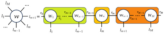
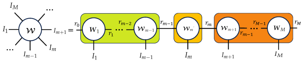
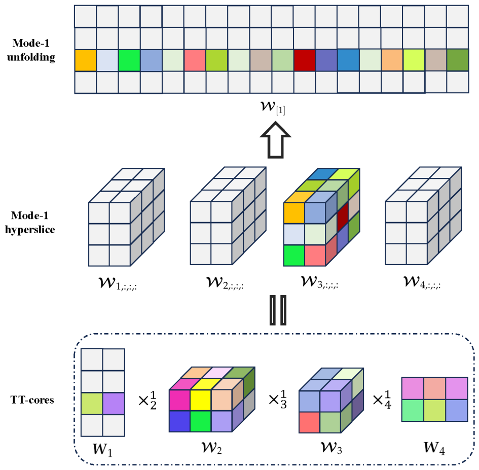
By factorizing the high-order tensor $\mathcal{W}$ into a sequence of low-order interconnected cores, as shown in Figure 1, TT decomposition ensures that storage and computational complexity scales as $\mathcal{O}\left(M\right)$ [15].

Figure 1. Illustration of the TT decomposition. $\mathcal{W}=〚{\mathit{W}}_1,{\mathcal{W}}_2,\dots ,{\mathcal{W}}_{M-1},{\mathit{W}}_M〛.$ $r_0=r_M=1.$

Here, we propose a novel sparse optimization model based on TT decomposition. Compared to the numerical instability of CP and the dimensionality curse of Tucker, the TT format provides a stable and highly compact representation with $\mathcal{O}(M\overline{I}{\overline{r}}^2+2\overline{r}\overline{I}-2\overline{I}{\overline{r}}^2)$ parameters, effectively avoiding the curse of dimensionality and enabling more scalable and efficient sparse optimization for high-order tensors. The linear tensor network underlying the TT decomposition inherently reflects local dependence along an ordered mode direction in the real-world data (e.g., time, space, and frequency), which resonates with the smoothness structure assumed along the domain in functional data analysis. In contrast, CP decomposes the tensor into a symmetric sum of rank-one terms with no notion of ordering, while Tucker, despite introducing a core tensor, still treats all modes symmetrically and thus similarly lacks this sequential locality.

Within tensor-decomposition frameworks, directly imposing sparsity on the core factors has emerged as a natural and effective strategy for feature selection [19,20,21]. For example, Ahmed et al. [19] proposed a tensor-structured regression model that achieves precise feature selection by directly imposing ${\mathcal{l}}_0$-norm sparsity constraints on the factor matrices within a Tucker decomposition framework. Their work demonstrated that characterizing sparsity at the factor level drastically reduces the parameter degrees of freedom, thereby improving sample complexity and facilitating model interpretability. Similarly, Chen and Luo [21] established the equivalence between frontal slice sparsity in a third-order tensor and row sparsity of the factor matrix corresponding to the third mode in the CP decomposition. This equivalence simultaneously achieves computational reduction through structural factorization and feature selection via sparsity. This paradigm of performing variable selection at the level of a structured coefficient block, rather than individual scalar coefficients, shares a profound methodological connection with functional data analysis [22]. In functional contexts, excluding a predictor requires setting its entire coefficient function to zero, a principle successfully addressed by structured penalties such as the adaptive function-on-scalar Lasso [23]. Motivated by this concept of structured blockwise selection, we aim to extend this property to high-dimensional tensor-on-tensor regression. In this paper, the primary objective of tensor-on-tensor regression modeling is to efficiently determine the high-order tensor estimator with mode-1 hyperslice sparsity (see Section 2) using a minimal number of training observations, ${\left\{({\mathcal{X}}_n,{\mathcal{Y}}_n)\right\}}_{n=1}^N$. To achieve this while maintaining computational efficiency, we leverage TT decomposition by directly imposing the sparsity of the high-order tensor $\mathcal{W}$ on the first core factor, ${\mathit{W}}_1$, which is equivalent to the mode-1 hyperslice sparsity in $\mathcal{W}$ (see Section 3). Furthermore, to statistically guarantee that the feature selection properties induced by this sparsity can be faithfully mapped back to the original high-order tensor, we enforce orthogonality constraints on the remaining $M-1$ core tensors.

In this paper, we propose the following Sparse Tensor Train Optimization via Orthogonal Decomposition (STOD) optimization:

$$\begin{array}{cc}\hfill \underset{{\mathit{W}}_1,{\left\{{\mathcal{W}}_i\right\}}_{i=2}^{M-1},{\mathit{W}}_M}{\min }& {\displaystyle \frac{1}{2}}\parallel \mathcal{Y}-〚{\mathit{W}}_1,{\left\{{\mathcal{W}}_i\right\}}_{i=2}^{M-1},{\mathit{W}}_M〛{\times }_{1,2,\dots ,m}^{1,2,\dots ,m}{\mathcal{X}\parallel }_F^2+\lambda {\parallel {\mathit{W}}_1\parallel }_{2,0}\hfill \\ \hfill \mathrm{s}.\mathrm{t}.& (\mathfrak{L}{\left({\mathcal{W}}_2\right)}^{\mathsf{T}},\dots ,\mathfrak{L}{\left({\mathcal{W}}_{M-1}\right)}^{\mathsf{T}},{\mathit{W}}_M^{\mathsf{T}})\hfill \\ \hfill & \in \mathrm{St}(I_2{r}_2,r_1)\times \cdots \times \mathrm{St}(I_{M-1}{r}_{M-1},r_{M-2})\times \mathrm{St}(I_M,r_{M-1}),\hfill \end{array}$$

(2)

where $\mathcal{X}\in {\mathbb{R}}^{I_1\times \cdots \times I_m\times N}$, $\mathcal{Y}\in {\mathbb{R}}^{I_{m+1}\times \cdots \times I_M\times N},$${\mathit{W}}_1\in {\mathbb{R}}^{I_1\times r_1},$${\mathit{W}}_M\in {\mathbb{R}}^{r_{M-1}\times I_M},$${\mathcal{W}}_i\in {\mathbb{R}}^{r_{i-1}\times I_i\times r_i}$, $i=2,3,\dots ,M-1$, and $\mathfrak{L}\left({\mathcal{W}}_i\right)$ is defined as

$$\mathfrak{L}\left({\mathcal{W}}_i\right)=[{\mathit{W}}_i(:,1,:),\dots ,{\mathit{W}}_i(:,I_i,:)]\in {\mathbb{R}}^{r_{i-1}\times \left(I_i{r}_i\right)},$$

with ${\mathit{W}}_i(:,1,:)$ being a lateral slice of ${\mathcal{W}}_i$. St$(r_i{I}_i,r_{i-1}):=\{\mathfrak{L}{\left({\mathcal{W}}_i\right)}^{\mathsf{T}}\in {\mathbb{R}}^{r_i{I}_i\times r_{i-1}}:\mathfrak{L}\left({\mathcal{W}}_i\right)\mathfrak{L}{\left({\mathcal{W}}_i\right)}^{\mathsf{T}}={\mathit{I}}_{r_{i-1}}\}$ is the Stiefel manifold. Given a matrix, $\mathit{A}\in {\mathbb{R}}^{I_1\times r_1}$, denote ${\parallel \mathit{A}\parallel }_{2,0}:=♯\{j\in \left[I_1\right]:\parallel {\mathit{a}}_{j:}{\parallel }_2\ne 0\}.$ Building upon this novel optimization (2), our formulation successfully decouples the high-dimensional feature selection task into a highly efficient TT decomposition. The identifiability of sparse coefficients in structured representations traces back to (Corollary 1 [24]). This work established a theoretical guarantee for underdetermined linear systems. Specifically, a sufficiently sparse solution is uniquely identified when its sparsity level is less than half the spark of the dictionary. This fundamental reasoning has been extended for decomposable tensor regression frameworks in [21], which demonstrated that, under a sufficiently sparse frontal-slice structure and mild rank conditions on the loading matrices, the coefficient tensor within a CP decomposition regression model achieves global identifiability. This foundational conclusion can also be naturally extended to our proposed model.

Achieving computational efficiency and scalability in evaluating tensor-on-tensor regression models has also garnered widespread attention. Qin et al. [16] proposed two first-order optimization algorithms, namely Iterative Hard Thresholding (IHT) and Riemannian Gradient Descent (RGD), to solve the optimization model and establish the upper and minimax lower bounds for parameter estimation in TT-based optimization under the restricted isometry property. Hu and Chen [25] addressed the sparse TT decomposition problem by incorporating an ${\mathcal{l}}_1$-norm regularization term. The proximal alternating linearized minimization (PALM) algorithm is employed to solve the problem. Inspired by [26], we further develop an efficient alternating optimization algorithm with a preconditioned metric. The primary contributions of this paper are threefold:

(1)

We introduce an ${\mathcal{l}}_{2,0}$-norm regularization on the first TT-core ${\mathit{W}}_1$. We establish a mathematical equivalence between the mode-1 hyperslice sparsity of $\mathcal{W}$ and the ${\mathcal{l}}_{2,0}$-norm sparsity of ${\mathit{W}}_1$. This structural equivalence theoretically guarantees the accuracy of feature selection.

(2)

We introduce an Alternating Proximal and Preconditioned Riemannian Gradient Descent (AP2RGD) method equipped with a preconditioned metric by exploiting the second-order information of the orthogonal variables. Furthermore, we theoretically guarantee that the optimization algorithm converges to a critical point.

(3)

Extensive numerical experiments on both synthetic and real-world datasets demonstrate the feasibility of the proposed model and the computational effectiveness of the alternating algorithm.

The remainder of the paper is organized as follows. In Section 2, we review basic tensor concepts and nonsmooth analysis for the ${\mathcal{l}}_{2,0}$-norm and Stiefel manifold. Section 3 develops the equivalence between the group sparsity of ${\mathit{W}}_1$ and the mode-1 hyperslice sparsity of $\mathcal{W}$ and establishes uniform variable-selection consistency. In Section 4, we introduce an alternating optimization algorithm to solve the STOD optimization model, and we prove that it converges to a critical point. In Section 5, we conduct comparative numerical experiments to validate the effectiveness of our proposed approach. Conclusions are drawn in Section 6.

2. Preliminaries

This section introduces some notations and nonsmooth analysis tools.

2.1. Notations and Tensor Basis

We denote scalars, vectors, matrices and tensors by lowercase letters and uppercase letters (e.g., $a,$ b, A, B), boldface lowercase letters (e.g., $\mathit{a},$ $\mathit{b}$), boldface uppercase letters (e.g., $\mathit{A},$ $\mathit{B}$), and boldface calligraphic letters (e.g., $\mathcal{A},$ $\mathcal{B}$), respectively. $\mathbb{N}$ denotes the set of natural numbers. Given a matrix, $\mathit{A}=[{\mathit{a}}_1,{\mathit{a}}_2,...,{\mathit{a}}_m]\in {\mathbb{R}}^{p\times m}$, the vectorization $\mathrm{vec}\left(\mathit{A}\right)$ is defined as $[{\mathit{a}}_1;{\mathit{a}}_2;...;{\mathit{a}}_m]$; ${\mathrm{vec}}^{-1}(·)$ is its inverse operation. Denote $\left[p\right]:=\{1,2,\dots ,p\}$. Define the row support set of $\mathit{A}$ by $\mathrm{supp}\left(\mathit{A}\right):=\{i\in \left[p\right]|\parallel {\mathit{a}}_{i:}{\parallel }_2\ne 0\}$, with $\parallel {\mathit{a}}_{i:}{\parallel }_2$ being the Euclidean norm. ${\parallel \mathit{A}\parallel }_F$ denotes the Frobenius norm of $\mathit{A}$.

An Nth-order tensor $\mathcal{A}\in {\mathbb{R}}^{I_1\times I_2\times \dots \times I_N}$ with $(i_1,i_2,\dots ,i_N)$th entry is denoted as $a_{i_1,i_2,\dots ,i_N}$, where $i_n=1,2,\dots ,I_n$ for all $n\in \left[N\right]:=\{1,2,\dots ,N\}$. In particular, vectors and matrices are considered low-order tensors with $N=1$ and $N=2$, respectively. The mode-k hyperslice of tensor $\mathcal{A}$ is a $(N-1)$th-order tensor of size $I_1\times \cdots \times I_{k-1}\times I_{k+1}\times \cdots \times I_N$. The jth mode-k hyperslice is given by $\mathcal{A}(:,\dots ,:,j,:,\dots ,:)$. The  mode-k hyperslice sparsity is defined as

$$\parallel \begin{array}{c}\hfill \mathcal{A}\end{array}{\parallel }_{m_k,0}=♯\{j\in \left[I_k\right]|\parallel \mathcal{A}(:,\dots ,:,j,:,\dots ,:){\parallel }_F\ne 0\}.$$

Table 1 lists the tensor operations utilized in this study, which include the contraction product, mode-n unfolding, k-unfolding, and mode-permuted tensor. The specific formulations for these operations are provided in Appendix A.

Table 1. Basic tensor operations.

Notations	Descriptions
${\times }_{s,s+1,\dots ,t}^{s,s+1,\dots ,t}$	contraction product; see (A1)
${\mathcal{A}}_{\left[n\right]}$	mode-n unfolding; see (A2)
${\mathcal{A}}_{⟨k⟩}$	k-unfolding; see (A3)
${\mathcal{T}}_{\pi \left(1\right),\dots ,\pi \left(N\right)}\left(\mathcal{A}\right)$	mode-permuted tensor; see (A4)

2.2. Nonsmooth Analysis

The fundamental notions and concepts used below follow the monograph [27] and the properties of ${\mathcal{l}}_{2,0}$-norm discussed in [28]. For a proper, closed function, $g:{\mathbb{R}}^{P\times Q}\to (-\infty ,\infty ]$, the subdifferential and the proximal operator of g are recalled below.

The proximal operator of g is given by

$${\mathrm{Prox}}_{\lambda g(·)}\left(\mathit{X}\right):=\arg \underset{\mathit{Z}}{\min }\left\{\lambda g\left(\mathit{Z}\right)+{\displaystyle \frac{1}{2}}{\parallel \mathit{Z}-\mathit{X}\parallel }_F^2\right\},\forall \mathit{X}\in {\mathbb{R}}^{P\times Q}.$$

(3)

Specifically, the proximal operator of ${\parallel ·\parallel }_{2,0}$ takes the following form:

$$\begin{array}{c}{\left[{\mathrm{Prox}}_{{\lambda \parallel ·\parallel }_{2,0}}\left(\mathit{X}\right)\right]}_{i:}=\left\{\begin{array}{cc}\left\{{\mathit{x}}_{i:}\right\},\hfill & \mathrm{if}\parallel {\mathit{x}}_{i:}{\parallel }_2>\sqrt{2\lambda }\hfill \\ \{{\mathit{x}}_{i:},\mathbf{0}\},\hfill & \mathrm{if}\parallel {\mathit{x}}_{i:}{\parallel }_2=\sqrt{2\lambda }\hfill \\ \left\{\mathbf{0}\right\},\hfill & \mathrm{if}\parallel {\mathit{x}}_{i:}{\parallel }_2<\sqrt{2\lambda }\hfill \end{array},\right.i\in \left[P\right].\hfill \end{array}$$

The indicator function of a set, $\mathbb{C}\subseteq {\mathbb{R}}^{P\times Q}$, denoted as ${\delta }_{\mathbb{C}}$, is defined by

$${\delta }_{\mathbb{C}}\left(\mathit{X}\right)=0,\mathrm{if}\mathit{X}\in \mathbb{C},{\delta }_{\mathbb{C}}\left(\mathit{X}\right)=\infty ,\mathrm{if}\mathit{X}\notin \mathbb{C}.$$

The subdifferential of ${\delta }_{\mathrm{St}(P,Q)}$ at any $\mathit{X}\in \mathrm{St}(P,Q)$ is given as follows:

$$\partial {\delta }_{\mathrm{St}(P,Q)}\left(\mathit{X}\right)=\left\{\mathit{X}\mathit{S}|\mathit{S}={\mathit{S}}^{\mathsf{T}},\mathit{S}\in {\mathbb{S}}^{Q\times Q}\right\},$$

(4)

The proximal operator of ${\delta }_{\mathrm{St}(P,Q)}$ is exactly the projection operator onto $\mathrm{St}(P,Q)$, which takes the form

$${\mathcal{P}}_{\mathrm{St}(P,Q)}\left(\mathit{X}\right)=\mathit{U}{\mathit{V}}^{\mathsf{T}},$$

(5)

where $\mathit{U}\in {\mathbb{R}}^{P\times Q},\mathit{V}\in {\mathbb{R}}^{Q\times Q}$ are the column-orthogonal matrices from the SVD of $\mathit{X}$.

3. Statistical Results

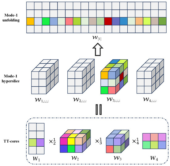
This section establishes the theoretical guarantees for both the uniform variable-selection consistency for $\mathcal{W}$ and the oracle estimation consistency. The theoretical development hinges on the equivalence between the row-sparsity of the first TT-core ${\mathit{W}}_1$ and the mode-1 hyperslice sparsity of the high-order estimator $\mathcal{W}$, as depicted in Figure 2. This implies that $\mathrm{supp}\left(\mathcal{W}\right)=\mathrm{supp}\left({\mathit{W}}_1\right),$ where $\mathrm{supp}\left(\mathcal{W}\right):=\{j\in \left[I_1\right]:\parallel \mathcal{W}(j,:,\dots ,:){\parallel }_F\ne 0\}.$

Figure 2. Illustration of the equivalence between the group sparsity of ${\mathit{W}}_1$ and the mode-1 hyperslice sparsity of $\mathcal{W}.$ Here, $\mathcal{W}\in {\mathbb{R}}^{4\times 2\times 2\times 3}.$ $\mathit{r}=(2,2,2).$ ${\parallel \mathcal{W}\parallel }_{m_1,0}={\parallel {\mathit{W}}_1\parallel }_{2,0}=1.$ $\mathrm{supp}\left(\mathcal{W}\right)=\mathrm{supp}\left({\mathit{W}}_1\right)=\left\{3\right\}.$ Also, the elements of matrices and tensors are zero (gray) and nonzero (color).

The motivation for our theoretical development stems from functional data analysis [22], where variable selection operates strictly on structured blocks to achieve oracle properties [23]. Inspired by this blockwise selection, the following derivations are dedicated to proving that our discrete ${\mathcal{l}}_{2,0}$ penalty, combined with TT decomposition, effectively translates this oracle estimation capability to high-dimensional tensor-on-tensor regression. To facilitate reading, we list some of the notations used in this section in Table 2.

Table 2. Some notations used in statistical analysis.

Notations	Descriptions
${\mathbb{S}}_{\mathit{r},s_0}$	orthogonally constrained sparse TT set
${\mathcal{W}}^{\mathrm{R}},{\mathcal{W}}_i^{\mathrm{R}}$	ground truth
$\mathfrak{L}\left({\mathcal{W}}_i\right)$	$[{\mathit{W}}_i(:,1,:),\dots ,{\mathit{W}}_i(:,I_i,:)]$
${\mathcal{W}}_{\ge 2}^{\mathrm{R}}$	(M-1)-order tensor obtained by the contraction sequence from ${\mathcal{W}}_2^{\mathrm{R}}$ to ${\mathit{W}}_M^{\mathrm{R}}$
${\mathcal{W}}_{\left[1\right]}^{\mathrm{R}}$	mode-1 unfolding of ${\mathcal{W}}^{\mathrm{R}}$
${\left({\mathcal{W}}_{\left[1\right]}^{\mathrm{R}}\right)}_{j:}$	the j-th row of the mode-1 unfolding matrix of tensor ${\mathcal{W}}^{\mathrm{R}}$
$C_{\min }\left({\mathcal{W}}^{\mathrm{R}}\right)$	, a measure of separation between the ground-truth parameter and the least favorable candidate model
${\eta }_{\min }\left({\mathcal{W}}^{\mathrm{R}}\right)$	the minimum row-wise signal strength of the true parameter
${\mathcal{W}}^i$	the element of the least-favorable set
$D_{\mathrm{KL}}({\mathcal{W}}^i,{\mathcal{W}}^j)$	Kullback-Leibler (KL) divergence

Definition 1

(Orthogonally Constrained Sparse TT Set). Let $\mathit{r}=(r_1,r_2,\dots ,r_{M-1})$ be the TT rank vector and $\parallel {\mathit{W}}_1^R{\parallel }_{2,0}=s_0$. The orthogonally constrained sparse TT set ${\mathbb{S}}_{\mathit{r},s_0}$ is defined as:

$$\begin{array}{c}\hfill {\mathbb{S}}_{\mathit{r},s_0}=\{{\mathcal{W}}^R\in {\mathbb{R}}^{I_1\times \cdots \times I_M}|{\mathcal{W}}^R=〚{\mathit{W}}_1^R,{\left\{{\mathcal{W}}_i^R\right\}}_{i=2}^{M-1},{\mathit{W}}_M^R〛,{\parallel {\mathit{W}}_1^R\parallel }_{2,0}=s_0,\\ \hfill \mathfrak{L}{\left({\mathcal{W}}_i^R\right)}^{\mathsf{T}}\in \mathit{St}(I_i{r}_i,r_{i-1}),i=2,\dots ,M-1,{\left({\mathit{W}}_M^R\right)}^{\mathsf{T}}\in \mathit{St}(I_M,r_{M-1})\}.\end{array}$$

(6)

Proposition 1.

Suppose that $\mathfrak{L}{\left({\mathcal{W}}_i\right)}^{\mathsf{T}}\in \mathit{St}(I_i{r}_i,r_{i-1})$, for each $i=2,\dots ,M-1,$ ${\mathit{W}}_M^{\mathsf{T}}\in \mathrm{St}(I_M,r_{M-1})$. Define

$$\overline{\mathcal{W}}={\mathcal{W}}_i{\times }_3^1{\mathcal{W}}_{i+1},i=2,\dots ,M-1.$$

Here, we use ${\mathit{W}}_M$ to denote the terminal core ${\mathcal{W}}_M.$ Then, we have

$${\overline{\mathcal{W}}}_{\left[1\right]}^{\mathsf{T}}\in \mathrm{St}(I_i{I}_{i+1}{r}_{i+1},r_{i-1}).$$

The proof of Proposition 1 is provided in Appendix B. The conclusion derived in Proposition 1 serves as the base case for a broader structural property. By induction over the sequence of mode contractions, it is straightforward to generalize this orthogonal constraint. Therefore, for any ${\mathcal{W}}^{\mathrm{R}}=〚{\mathit{W}}_1^{\mathrm{R}},{\left\{{\mathcal{W}}_i^{\mathrm{R}}\right\}}_{i=2}^{M-1},{\mathit{W}}_M^{\mathrm{R}}〛\in {\mathbb{S}}_{\mathit{r},s_0}$, it naturally follows that

$${\left({\mathcal{W}}_{\ge 2}^{\mathrm{R}}\right)}_{\left[1\right]}^{\mathsf{T}}\in \mathrm{St}({\Pi }_{i=2}^M{I}_i,r_1),$$

(7)

where

$$\begin{array}{ccc}{\mathcal{W}}_{\ge 2}^{\mathrm{R}}& =& 〚{\mathcal{W}}_2^{\mathrm{R}},\dots ,{\mathit{W}}_M^{\mathrm{R}}〛\hfill \\ & =& {\mathcal{W}}_2^{\mathrm{R}}{\times }_3^1{\mathcal{W}}_3^{\mathrm{R}}{\times }_4^1\cdots {\times }_i^1{\mathcal{W}}_i^{\mathrm{R}}{\times }_{i+1}^1\cdots {\times }_M^1{\mathit{W}}_M^{\mathrm{R}}.\hfill \end{array}$$

It follows from ${\mathcal{W}}_{\left[1\right]}^{\mathrm{R}}={\mathit{W}}_1^{\mathrm{R}}{\left({\mathcal{W}}_{\ge 2}^{\mathrm{R}}\right)}_{\left[1\right]}$ and (7) that

$$\parallel {\left({\mathcal{W}}_{\left[1\right]}^{\mathrm{R}}\right)}_{j:}{\parallel }_2={\parallel {\left({\mathit{W}}_1^{\mathrm{R}}\right)}_{j:}\parallel }_2,\forall j\in \left[I_1\right].$$

(8)

Remark 1.

Let $\mathcal{W}\in {\mathbb{R}}^{I_1\times \cdots \times I_M}$ be a tensor with exact TT-ranks $\{r_1,\dots ,r_{M-1}\}$. Suppose that $\mathcal{W}$ admits two representations in the constrained TT format, denoted by $〚{\mathit{W}}_1,{\left\{{\mathcal{W}}_i\right\}}_{i=2}^{M-1},{\mathit{W}}_M〛$ and $〚{\mathit{W}}_1^{\prime },{\left\{{\mathcal{W}}_i^{\prime }\right\}}_{i=2}^{M-1},{\mathit{W}}_M^{\prime }〛$, with both satisfying the right-orthogonality constraints as defined in (2). Then, there exist orthogonal matrices ${\mathcal{Q}}_i$ for $i=1,\dots ,M-1$, such that the two representations are related by gauge transformations. Consequently, $\mathit{supp}\left({\mathit{W}}_1\right)=\mathit{supp}\left({\mathit{W}}_1^{\prime }\right)$, and this row-sparsity pattern uniquely coincides with the mode-1 hyperslice support of $\mathcal{W}$.

To quantify the difficulty of support recovery, we introduce a measure of separation between the ground-truth parameter and the least favorable candidate model, which is described as

$$C_{\min }\left({\mathcal{W}}^{\mathrm{R}}\right)=\underset{\begin{array}{c}\mathcal{W}:\mathcal{W}\ne \mathrm{supp}\left({\mathcal{W}}^{\mathrm{R}}\right)\\ \left|\mathrm{supp}\left(\mathcal{W}\right)\right|\le \alpha s_0\end{array}}{\inf }{\displaystyle \frac{h^2(\mathcal{W},{\mathcal{W}}^{\mathrm{R}})}{\max \left(\right|\mathrm{supp}\left({\mathcal{W}}^{\mathrm{R}}\right)\setminus \mathrm{supp}\left(\mathcal{W}\right)|,1)}},$$

where $\alpha >1$, $|·|$ and ∖ denote set cardinality and set difference, respectively, and

$$h^2(\mathcal{W},{\mathcal{W}}^{\mathrm{R}})=1-\exp (-{\displaystyle \frac{1}{8{\sigma }^2}}\parallel (\mathcal{W}-{\mathcal{W}}^{\mathrm{R}}){\times }_{1,2,\dots ,m}^{1,2,\dots ,m}\mathcal{X}{\parallel }_F^2)$$

with $h(\mathcal{W},{\mathcal{W}}^{\mathrm{R}})$ being the Hellinger distance. By virtue of the property established in (8), the minimum row-wise signal strength of the true parameter can be defined as

$${\eta }_{\min }\left({\mathcal{W}}^{\mathrm{R}}\right):=\underset{j\in \mathrm{supp}\left({\mathcal{W}}^{\mathrm{R}}\right)}{\min }\parallel {\left({\mathcal{W}}_{\left[1\right]}^{\mathrm{R}}\right)}_{j:}{\parallel }_2=\underset{j\in \mathrm{supp}\left({\mathit{W}}_1^{\mathrm{R}}\right)}{\min }{\parallel {\left({\mathit{W}}_1^{\mathrm{R}}\right)}_{j:}\parallel }_2=:{\eta }_{\min }\left({\mathit{W}}_1^{\mathrm{R}}\right).$$

Equation (8) yields

$${\parallel \mathcal{W}\parallel }_{m_1,0}:={♯\left\{i\right|\parallel \mathcal{W}(i,:,\dots ,:)\parallel }_F\ne 0,i\in \left[I_1\right]\}=\parallel {\mathit{W}}_1{\parallel }_{2,0}.$$

We construct an approximated least-favorable parameter class for feature selection,

$${\mathcal{W}}_{m_1,0}(lb,ub):=\{\mathcal{W}\in {\mathbb{R}}^{I_1\times \cdots \times I_M},C_{\min }\left(\mathcal{W}\right)\ge {lb,\parallel \mathcal{W}\parallel }_{m_1,0}\le ub\},$$

where $0<ub\le \min \{N,I_1\}$ and $lb>0$. We construct the approximated least-favorable set $\Theta =\{{\mathcal{W}}^0,{\mathcal{W}}^1,\dots ,{\mathcal{W}}^{I_1}\}$ as described in [29]. Based on TT decomposition, we define ${\mathcal{W}}^j=〚{\mathit{W}}_1^j,{\left\{{\mathcal{W}}_i^j\right\}}_{i=2}^{M-1},{\mathit{W}}_M^j〛$, $j=0,1,\dots ,I_i$. ${\mathit{W}}_1^0$ is defined, such that $\parallel {\left({\mathit{W}}_1^0\right)}_{j:}{\parallel }_2={\eta }_{\min }\left({\mathcal{W}}^{\mathrm{R}}\right)$ for all $j\in \mathrm{supp}\left({\mathit{W}}_1^{\mathrm{R}}\right)$ and $\parallel {\left({\mathit{W}}_1^0\right)}_{j:}{\parallel }_2=0$ for $j\in \left[I_1\right]\setminus \mathrm{supp}\left({\mathit{W}}_1^{\mathrm{R}}\right).$ For each $i\in \left[I_i\right],$

$$\left\{\begin{array}{c}\parallel {\left({\mathit{W}}_1^i\right)}_{j:}{\parallel }_2={\eta }_{\min }\left({\mathcal{W}}^{\mathrm{R}}\right),j\in \mathrm{supp}\left({\mathit{W}}_1^{\mathrm{R}}\right)\setminus \left\{i\right\},\hfill \\ \parallel {\left({\mathit{W}}_1^i\right)}_{j:}{\parallel }_2=0,j\in \{\left[I_1\right]\setminus \mathrm{supp}\left({\mathit{W}}_1^{\mathrm{R}}\right)\}\cup \left\{i\right\},\hfill \end{array}\right.i\le s_0,$$

(9)

and

$$\left\{\begin{array}{c}\parallel {\left({\mathit{W}}_1^i\right)}_{j:}{\parallel }_2={\eta }_{\min }\left({\mathcal{W}}^{\mathrm{R}}\right),j\in \mathrm{supp}\left({\mathit{W}}_1^{\mathrm{R}}\right)\cup \left\{i\right\},\hfill \\ \parallel {\left({\mathit{W}}_1^i\right)}_{j:}{\parallel }_2=0,j\in \{\left[I_1\right]\setminus \mathrm{supp}\left({\mathit{W}}_1^{\mathrm{R}}\right)\}\setminus \left\{i\right\},\hfill \end{array}\right.i>s_0.$$

(10)

By virtue of this construction, the factor matrices inherently satisfy $\mathfrak{L}{\left({\mathcal{W}}_k^i\right)}^{\mathsf{T}}\in \mathrm{St}(I_i{r}_i,r_{i-1}),$ ${\left({\mathit{W}}_M^i\right)}^{\mathsf{T}}\in \mathrm{St}(I_M,r_{M-1})$, $k=2,\dots ,M-1,$ $i=0,1,\dots ,I_1$.

The following proposition establishes the relationship between the elements of the least-favorable set and the minimum row-wise signal strength of the true parameter, ${\eta }_{\min }\left({\mathcal{W}}^{\mathrm{R}}\right)$. This relationship lays the theoretical foundation for the necessary condition under which (2) achieves uniform variable selection consistency.

Proposition 2.

For any ${\mathcal{W}}^i,{\mathcal{W}}^j\in \Theta ,i\ne j,$ the following inequality holds:

$$\parallel {\mathcal{W}}^i-{\mathcal{W}}^j{\parallel }_F\le (\sqrt{2}+\sqrt{I_1}b){\eta }_{\min }\left({\mathcal{W}}^{\mathrm{R}}\right),$$

(11)

where $b={\displaystyle \sum _{k=2}^{M-1}}\parallel {\mathcal{W}}_k^i-{\mathcal{W}}_k^j{\parallel }_F+{\parallel {\mathit{W}}_M^i-{\mathit{W}}_M^j\parallel }_F.$

The proof of Proposition 2 is shown in Appendix C. Building upon the theoretical results established in Proposition 2, we obtain the following upper bound for the Kullback–Leibler (KL) divergence

$$\begin{array}{ccc}{D}_{\mathrm{KL}}({\mathcal{W}}^i,{\mathcal{W}}^j)\hfill & =\hfill & {\displaystyle \frac{1}{2{\sigma }^2}}{\parallel ({\mathcal{W}}^i-{\mathcal{W}}^j){\times }_{1,2,\dots ,m}^{1,2,\dots ,m}\mathcal{X}\parallel }_F^2\hfill \\ \hfill & \le \hfill & {\displaystyle \frac{{\parallel \mathcal{X}\parallel }_F^2{(\sqrt{2}+\sqrt{I_1}b)}^2}{2{\sigma }^2}}{\eta }_{\min }^2\left({\mathcal{W}}^{\mathrm{R}}\right),\hfill \end{array}$$

for any ${\mathcal{W}}^i,{\mathcal{W}}^j\in \Theta ,i\ne j.$ Since the coefficient ${\parallel \mathcal{X}\parallel }_F^2{(\sqrt{2}+\sqrt{I_1}b)}^2/2{\sigma }^2>0$, this construction implies that a necessary condition for selection consistency takes the form $C_{\min }\left({\mathcal{W}}^{\mathrm{R}}\right)\ge \kappa {\displaystyle \frac{I_1}{N}}$ for a consistency constant $\kappa >0$ [30].

To quantify the local complexity of the model, we introduce the function class

$${\mathcal{W}}_S=\{f_s^{{\displaystyle \frac{1}{2}}}\left(\mathrm{vec}\left({\mathcal{Y}}_n\right)\right|\mathrm{vec}\left({\mathcal{X}}_n\right),{\mathcal{W}}_{⟨m⟩})\mid \mathcal{W}=({\mathcal{W}}_{S:};{\mathcal{O}}_{\left[I_1\right]\setminus S:}),h(\mathcal{W},{\mathcal{W}}^{\mathrm{R}})\le \epsilon \},$$

with $f_s(\mathrm{vec}\left({\mathcal{Y}}_n\right)\mid \mathrm{vec}\left({\mathcal{X}}_n\right),{\mathcal{W}}_{⟨m⟩})$ being the density function of Gaussian distribution given by

$$\mathcal{N}({\mathcal{W}}_{⟨m⟩}^{\mathsf{T}}\mathrm{vec}\left({\mathcal{X}}_n\right),{\sigma }^2{\mathit{I}}_{{\Pi }_{j=m+1}^M{I}_j}).$$

The bracketing Hellinger metric entropy of ${\mathcal{W}}_S$, denoted as $H(u,{\mathcal{W}}_S)$, is defined as the logarithm of the cardinality of the smallest u-bracketing of ${\mathcal{W}}_S$. It follows from [31] that $H(u,{\mathcal{W}}_S)\le c_0\left|S\right|\ln \left({\displaystyle \frac{\epsilon }{u}}\right)$ for $0<u<\epsilon \le 1$ and $\left|S\right|\le \alpha s_0$, where $c_0$ is a positive constant. Let ${\mathcal{W}}^{*}$ be a global minimizer of (2), and let ${\mathcal{W}}_{\mathrm{ML}}^{*}$ denote the oracle estimator.

Theorem 1.

If $\lambda \le c_{1}N/s_0$ and ${\displaystyle \frac{2\ln I_1+\ln (t^{(\alpha -1)s_0}+1)}{N{C}_{\min }\left({\mathcal{W}}^{\mathrm{R}}\right)}}<c_2$, we have

$$\mathrm{Pr}({\mathcal{W}}^{*}\ne {\mathcal{W}}_{\mathrm{ML}}^{*})\le \exp \left\{-c_{2}N{C}_{\min }\left({\mathcal{W}}^{\mathrm{R}}\right)+2\ln I_1+\ln (t^{(\alpha -1)s_0}+1)\right\},$$

(12)

where $c_1=1/24$, $c_2=2/26001$, and $t=I_1-s_0$. Furthermore, if the consistency constant satisfies $\kappa >(2+(\alpha -1)s_0)/c_2$, then the following properties hold:  

(i) 

Reconstruction of the oracle estimator:

$$\underset{N\to \infty }{\lim }\mathrm{Pr}\left({\mathcal{W}}^{*}={\mathcal{W}}_{\mathit{ML}}^{*}\right)=1.$$

(ii) 

Uniform variable-selection consistency:

$$\underset{N\to \infty }{\lim }\underset{{\mathcal{W}}^R\in {\mathcal{W}}_{m_1,0}(lb,ub)}{\sup }\mathrm{Pr}(\mathit{supp}\left({\mathcal{W}}^{*}\right)=\mathit{supp}\left({\mathcal{W}}^R\right))=1.$$

The proof follows a similar procedure to that of Theorem 1 in [30].

Remark 2.

Theorem 1 (ii) ensures mode-1 hyperslice support recovery, while (i) guarantees oracle estimator reconstruction. These findings generalize back to functional tensor regression [32]. The ${\mathcal{l}}_{2,0}$-norm sparsity on ${\mathit{W}}_1$ naturally converges to the exclusion of entire coefficient functions as dimensions approach infinity. Thus, STOD extends structured blockwise selection and its oracle properties to functional tensor regression.

4. The Solution Approach

In this section, we rigorously analyze the optimality conditions of the optimization model (2). To efficiently solve this problem, we propose an Alternating Proximal and Preconditioned Riemannian Gradient Descent algorithm (AP2RGD) and subsequently establish its theoretical convergence to a critical point. For the reader’s convenience, a summary of the notations in this section is shown in Table 3.

Table 3. Some notations used in optimality analysis and algorithm.

Notations	Descriptions
$g_{{\mathcal{W}}_i}({\xi }_i,{\mathit{\eta }}_i)$	a metric on a manifold
$\overline{\mathit{H}},{\overline{\mathit{H}}}_i\left({\mathcal{W}}_i\right),{\overline{\mathit{H}}}_i$	a self-adjoint positive-definite linear operator
${\mathrm{grad}}_{g,{\mathcal{W}}_i}h(·)$	the Riemannian gradient of h
${\nabla }_{{\mathcal{W}}_i}h(·)$	the gradient of h with respect to ${\mathcal{W}}_i$
${\mathcal{T}}_{{\mathcal{W}}_i}\mathrm{St}(I_i{r}_i,r_{i-1})$	the tangent space to $\mathrm{St}(I_i{r}_i,r_{i-1})$ at ${\mathcal{W}}_i$
${\mathrm{Retr}}_{{\overline{\mathcal{W}}}^k}\left(s^k{\overline{\mathit{\eta }}}^k\right)$	a retraction on a manifold

4.1. Optimality

To facilitate subsequent analysis, we first present the explicit expressions for the gradient and Hessian of the loss function. For notational simplicity, we denote $h({\mathit{W}}_1,{\left\{{\mathcal{W}}_i\right\}}_{i=2}^{M-1},{\mathit{W}}_M)={\displaystyle \frac{1}{2}}\parallel \mathcal{Y}-〚{\mathit{W}}_1,{\left\{{\mathcal{W}}_i\right\}}_{i=2}^{M-1},{\mathit{W}}_M〛{\times }_{1,2,\dots ,m}^{1,2,\dots ,m}\mathcal{X}{\parallel }_F^2.$

Property 1.

(i) The contraction product term in (2) can be equivalently reformulated as follows:

$$\begin{array}{cc}\hfill & 〚{\mathit{W}}_1,{\left\{{\mathcal{W}}_i\right\}}_{i=2}^{M-1},{\mathit{W}}_M〛{\times }_{1,2,\dots ,m}^{1,2,\dots ,m}\mathcal{X}\hfill \\ \hfill & ={\mathcal{T}}_{[M-m,M-m-1,\dots ,1,M-m+1]}\left({\mathit{W}}_M{\times }_1^2(\cdots {\times }_1^2\left({\mathcal{W}}_{m+1}{\times }_1^1{\mathcal{G}}_1\right))\right)\hfill \end{array}$$

with

$${\mathcal{G}}_1={\mathcal{W}}_m{\times }_{1,2}^{1,2}(\cdots {\times }_{1,2}^{1,2}\left({\mathcal{W}}_2{\times }_{1,2}^{1,2}\left({\mathit{W}}_1{\times }_1^1\mathcal{X}\right)\right)).$$

(ii) The gradient of function h can be evaluated using two approaches.

■

Approach 1. The gradient of function h with respect to ${\mathcal{W}}_i$ (for $i=2,\dots ,M-1$) is given by

$${\nabla }_{{\mathcal{W}}_i}h({\mathit{W}}_1,{\left\{{\mathcal{W}}_i\right\}}_{i=2}^{M-1},{\mathit{W}}_M)={\mathcal{G}}_2,$$

where

$${\mathcal{G}}_2={\mathcal{G}}_3{\times }_{M-i+2}^2{\mathit{W}}_M{\times }_{M-i+1,M-i+2}^{2,3}{\mathcal{W}}_{M-1}{\times }_{M-i,M-i+1}^{2,3}\cdots {\times }_{3,4}^{2,3}{\mathcal{W}}_{i+1}$$

with

$${\mathcal{G}}_3={\mathcal{W}}_{i-1}{\times }_{1,2}^{1,2}(\cdots {\times }_{1,2}^{1,2}\left({\mathit{W}}_1{\times }_1^1{\mathcal{G}}_4\right))$$

and

$${\mathcal{G}}_4=\mathcal{X}{\times }_{m+1}^{M-m+1}(〚{\mathit{W}}_1,{\left\{{\mathcal{W}}_i\right\}}_{i=2}^{M-1},{\mathit{W}}_M〛{\times }_{1,2,\dots ,m}^{1,2,\dots ,m}\mathcal{X}-\mathcal{Y}).$$

Furthermore, the gradients of h with respect to ${\mathit{W}}_1$ and ${\mathit{W}}_M$ are explicitly defined as

$${\nabla }_{{\mathit{W}}_1}h({\mathit{W}}_1,{\left\{{\mathcal{W}}_i\right\}}_{i=2}^{M-1},{\mathit{W}}_M)={\mathcal{G}}_4{\times }_M^2{\mathit{W}}_M{\times }_{M-1,M}^{2,3}{\mathcal{W}}_{M-1}{\times }_{M-2,M-1}^{2,3}\cdots {\times }_{2,3}^{2,3}{\mathcal{W}}_2,$$

and

$${\nabla }_{{\mathit{W}}_M}h({\mathit{W}}_1,{\left\{{\mathcal{W}}_i\right\}}_{i=2}^{M-1},{\mathit{W}}_M)={\mathcal{G}}_3.$$

■

Approach 2. The gradient of function h with respect to ${\mathcal{W}}_i$ (for $i\in \left[M\right]$) is given by the following two cases:

• Case I: For any $i\le m$, we have

  $$\begin{array}{cc}& {\nabla }_{{\mathcal{W}}_i}h({\mathit{W}}_1,{\left\{{\mathcal{W}}_i\right\}}_{i=2}^{M-1},{\mathit{W}}_M)\hfill \\ \hfill =& {\mathcal{G}}_2^{\prime }{\times }_3^{M-m+1}(〚{\mathit{W}}_1,{\left\{{\mathcal{W}}_i\right\}}_{i=2}^{M-1},{\mathit{W}}_M〛{\times }_{1,2,\dots ,m}^{1,2,\dots ,m}\mathcal{X}-\mathcal{Y}){\times }_{4,5}^{1,2}{\mathcal{W}}_{m+1}\hfill \\ & {\times }_{M-m+3,4}^{1,2}{\mathcal{W}}_{m+2}\cdots {\times }_{5,4}^{1,2}{\mathit{W}}_M,\hfill \end{array}$$

  where

  $${\mathcal{G}}_2^{\prime }={\mathcal{W}}_{i-1}{\times }_{1,2}^{1,2}(\cdots {\times }_{1,2}^{1,2}\left({\mathit{W}}_1{\times }_1^1\mathcal{X}\right)){\times }_3^2{\mathcal{W}}_{i+1}{\times }_{3,m-i+4}^{2,1}{\mathcal{W}}_{i+2}\dots {\times }_{3,6}^{2,1}{\mathit{W}}_M.$$
• Case II: For any $i=m+1,\dots ,M,$ we have

  $$\begin{array}{cc}& {\nabla }_{{\mathcal{W}}_i}h({\mathit{W}}_1,{\left\{{\mathcal{W}}_i\right\}}_{i=2}^{M-1},{\mathit{W}}_M)\hfill \\ \hfill =& \left({\mathcal{W}}_{i-1}{\times }_{1,2}^{1,2}(\cdots {\times }_{1,2}^{1,2}({\mathcal{W}}_{m+1}\times {\mathcal{G}}_3^{\prime }))\right){\times }_3^2{\mathcal{W}}_{i+1}{\times }_{M-i+3,3}^{1,2}{\mathcal{W}}_{i+2}\cdots {\times }_{5,3}^{1,2}{\mathit{W}}_M,\hfill \end{array}$$

  where

  $${\mathcal{G}}_3^{\prime }={\mathcal{W}}_m{\times }_{1,2}^{1,2}(\cdots {\times }_{1,2}^{1,2}\left({\mathit{W}}_1{\times }_1^1\mathcal{X}\right)){\times }_2^{M-m+1}(〚{\mathit{W}}_1,{\left\{{\mathcal{W}}_i\right\}}_{i=2}^{M-1},{\mathit{W}}_M〛{\times }_{1,2,\dots ,m}^{1,2,\dots ,m}\mathcal{X}-\mathcal{Y}).$$

In this paper, we adopt the second approach due to its computational efficiency.

(iii) The Hessian of function h with respect to ${\mathcal{W}}_i$ (for $i\in \left[M\right]$) is given by the following two cases:

• Case I: For any $i\le m$, we have

  $$\begin{array}{c}{\nabla }_{{\mathcal{W}}_i}^{2}h({\mathit{W}}_1,{\left\{{\mathcal{W}}_i\right\}}_{i=2}^{M-1},{\mathit{W}}_M)={\mathcal{T}}_{[1,2,3,6,5,4]}\left({\mathcal{G}}_5{\times }_{3,5,6,\dots ,M-m+4}^{M-m+3,M-m,M-m-1,\dots ,1}{\mathcal{G}}_6\right),\hfill \end{array}$$

  where

  $$\begin{array}{c}{\mathcal{G}}_5={\mathcal{W}}_{i-1}{\times }_{1,2}^{1,2}(\dots \left({\mathcal{W}}_2{\times }_{1,2}^{1,2}\left({\mathit{W}}_1{\times }_1^1\mathcal{X}\right)\right)){\times }_3^2{\mathcal{W}}_{i+1}\hfill \\ {\times }_{m-i+4,3}^{1,2}{\mathcal{W}}_{i+2}\cdots {\times }_{6,3}^{1,2}{\mathcal{W}}_m{\times }_5^1{\mathcal{W}}_{m+1}\cdots {\times }_{M-m+4}^1{\mathit{W}}_M\hfill \end{array}$$

  and

  $$\begin{array}{c}{\mathcal{G}}_6={\mathit{W}}_M{\times }_1^3{\mathcal{W}}_{M-1}{\times }_2^3\cdots {\times }_{M-i}^3{\mathcal{W}}_{i+1}{\times }_{M-i+1,\dots ,M-m+1}^{i+1,\dots ,m}\mathcal{X}{\times }_{M-m+2}^1{W}_1\hfill \\ {\times }_{M-m+2,M-m+i+1}^{2,1}{\mathcal{W}}_2\cdots {\times }_{M-m+2,M-m+5}^{2,1}{\mathcal{W}}_{i-1}.\hfill \end{array}$$
• Case II: For any $i=m+1,\dots ,M,$ we have

  $$\begin{array}{c}{\nabla }_{{\mathcal{W}}_i}^{2}h({\mathit{W}}_1,{\left\{{\mathcal{W}}_i\right\}}_{i=2}^{M-1},{\mathit{W}}_M)={\mathcal{T}}_{[1,5,2,4,6,3]}({\mathcal{G}}_7{\times }_{1,3,\dots ,i-m+1,i-m+3,\dots ,M-m+2}^{M-m+1,\dots ,M-i+1,M-i-1,\dots ,1}{\mathcal{G}}_8\circ {\mathit{I}}_{I_i}),\hfill \end{array}$$

  where

  $$\begin{array}{c}{\mathcal{G}}_7={\mathcal{W}}_{i-1}{\times }_1^2\dots \left({\mathcal{W}}_{m+2}{\times }_1^2\left({\mathcal{W}}_{m+1}{\times }_1^1({\mathcal{W}}_m{\times }_{1,2}^{1,2}\dots \left({\mathcal{W}}_2{\times }_{1,2}^{1,2}\left({\mathit{W}}_1{\times }_1^1\mathcal{X}\right)\right))\right)\right)\hfill \\ \circ {\mathcal{W}}_{i+1}{\times }_{i-m+4}^1{\mathcal{W}}_{i+2}\cdots {\times }_{M-m+2}^1{\mathit{W}}_M\hfill \end{array}$$

  and

  $$\begin{array}{c}{\mathcal{G}}_8={\mathit{W}}_M{\times }_1^3{\mathcal{W}}_{M-1}\cdots {\times }_{M-i}^3{\mathcal{W}}_{i+1}\circ \mathcal{X}{\times }_{M-i+2}^1{\mathit{W}}_1{\times }_{M-i+2,M+m-i+2}^{2,1}{\mathcal{W}}_2\hfill \\ {\times }_{M-i+2,M+m-i+1}^{2,1}\cdots {\times }_{M-i+2,M-i+5}^{2,1}{\mathit{W}}_m{\times }_{M-i+3}^1{\mathcal{W}}_{m+1}\cdots {\times }_{M-m+1}^1{\mathcal{W}}_{i-1}.\hfill \end{array}$$

We now characterize the first-order optimality conditions for (2). Following the framework in [26], the critical point of (2) is defined via the Riemannian gradient, which inherently depends on the chosen metric g. To elegantly capture the geometric structure of the objective function, we adopt the preconditioned metric proposed by [33]. By embedding the second-order information directly into this metric space, we can formulate the Riemannian gradient and the corresponding critical point of (2). We define a metric using a self-adjoint, positive-definite linear operator, $\overline{\mathit{H}}$, on the tangent bundle $\mathcal{TE}$, such that

$$g_{\tilde{\mathit{W}}}(\xi ,\eta )={\displaystyle \sum _{i=2}^M}{g}_{{\mathcal{W}}_i}({\xi }_i,{\eta }_i)=\stackrel{M}{\sum _{i=2}}\mathrm{tr}\left({\xi }_i^{\mathsf{T}}{\eta }_i{\overline{\mathit{H}}}_i\left({\mathcal{W}}_i\right)\right),{\xi }_i,{\eta }_i\in {\mathcal{T}}_{{\mathcal{W}}_i}\mathrm{St}(I_i{r}_i,r_{i-1}),$$

(13)

where $\mathcal{E}:=\mathrm{St}(I_2{r}_2,r_1)\times \cdots \times \mathrm{St}(I_{M-1}{r}_{M-1},r_{M-2})\times \mathrm{St}(I_M,r_{M-1}),$ and ${\overline{\mathit{H}}}_i\left({\mathcal{W}}_i\right)$ is a matrix defined by

$${\overline{\mathit{H}}}_i\left({\mathcal{W}}_i\right)=\left\{\begin{array}{cc}\hfill {\left({\mathcal{G}}_5\right)}_{\left[1\right]}{\left({\mathcal{G}}_5\right)}_{\left[1\right]}^{\mathsf{T}}+\delta {\mathit{I}}_{r_{i-1}},& \mathrm{if}i=1,\dots ,m,\hfill \\ \hfill {\left({\mathcal{G}}_7\right)}_{\left[2\right]}{\left({\mathcal{G}}_7\right)}_{\left[2\right]}^{\mathsf{T}}+\delta {\mathit{I}}_{r_{i-1}},& \mathrm{if}i=m+1,\dots ,M,\hfill \end{array}\right.$$

(14)

with ${\mathcal{G}}_5$ and ${\mathcal{G}}_7$ being defined in Property 1 and $\delta$ being a positive constant. It follows that ${\overline{\mathit{H}}}_i\left({\mathcal{W}}_i\right)$ is positive-definite. Therefore, the Riemannian gradient of h at $\mathfrak{L}{\left({\mathcal{W}}_i\right)}^{\mathsf{T}}\in \mathrm{St}(I_i{r}_i,r_{i-1})$ with respect to g can be computed using the following equation (Proposition 3.61 [34]):

$$\begin{array}{cc}\hfill & gra{d}_{g,{\mathcal{W}}_i}h({\mathit{W}}_1,{\left\{{\mathcal{W}}_j\right\}}_{j=2}^{M-1},{\mathit{W}}_M)\hfill \\ \hfill & ={\mathrm{Proj}}_{g,{\mathcal{W}}_i}\left(\mathcal{L}{\left({\nabla }_{{\mathcal{W}}_i}h({\mathit{W}}_1,{\left\{{\mathcal{W}}_j\right\}}_{j=2}^{M-1},{\mathit{W}}_M)\right)}^{\mathsf{T}}{\overline{\mathit{H}}}_i{\left({\mathcal{W}}_i\right)}^{-1}\right),i=2,\dots ,M,\hfill \end{array}$$

(15)

where ${\mathrm{Proj}}_{g,{\mathcal{W}}_i}(·)$ is an orthogonal projector. Before providing the definition of a critical point, we introduce the following subdifferentiability property.

Proposition 3.

Since the function h is continuously differentiable, for any $({\mathit{W}}_1,{\left\{{\mathcal{W}}_i\right\}}_{i=2}^{M-1},{\mathit{W}}_M)$, we have

$$\begin{array}{cc}& \partial \overline{f}({\mathit{W}}_1,{\left\{{\mathcal{W}}_i\right\}}_{i=2}^{M-1},{\mathit{W}}_M)\hfill \\ \hfill =& ({\nabla }_{{\mathit{W}}_1}h({\mathit{W}}_1,{\left\{{\mathcal{W}}_i\right\}}_{i=2}^{M-1},{\mathit{W}}_M)+\lambda \partial \parallel {\mathit{W}}_1{\parallel }_{2,0},\hfill \\ & gra{d}_{g,{\mathcal{W}}_2}h({\mathit{W}}_1,{\left\{{\mathcal{W}}_j\right\}}_{j=2}^{M-1},{\mathit{W}}_M),\dots ,gra{d}_{g,{\mathit{W}}_M}h({\mathit{W}}_1,{\left\{{\mathcal{W}}_j\right\}}_{j=2}^{M-1},{\mathit{W}}_M)),\hfill \end{array}$$

where $\overline{f}({\mathit{W}}_1,{\left\{{\mathcal{W}}_i\right\}}_{i=2}^{M-1},{\mathit{W}}_M)=h({\mathit{W}}_1,{\left\{{\mathcal{W}}_i\right\}}_{i=2}^{M-1},{\mathit{W}}_M)+\lambda {\parallel {\mathit{W}}_1\parallel }_{2,0}+{\displaystyle \sum _{i=1}^{M-1}}{\delta }_{\mathrm{St}(I_i{r}_i,r_{i-1})}\left({\mathcal{W}}_i\right)$ $+{\delta }_{\mathrm{St}(I_M,r_{M-1})}\left({\mathit{W}}_M\right).$

The proof of Proposition 3 can be found in Appendix D. We then introduce the definition of a critical point.

Definition 2.

A tuple $({\mathit{W}}_1^{*},{\left\{{\mathcal{W}}_i^{*}\right\}}_{i=2}^{M-1},{\mathit{W}}_M^{*})$ is a critical point if it satisfies the first-order optimality condition

$$\left\{\begin{array}{c}\mathit{O}\in {\nabla }_{{\mathit{W}}_1}h({\mathit{W}}_1^{*},{\left\{{\mathcal{W}}_i^{*}\right\}}_{i=2}^{M-1},{\mathit{W}}_M^{*})+\lambda \partial {\parallel {\mathit{W}}_1^{*}\parallel }_{2,0},\hfill \\ \mathit{O}={\mathit{grad}}_{g,{\mathcal{W}}_i}h({\mathit{W}}_1^{*},{\left\{{\mathcal{W}}_i^{*}\right\}}_{i=2}^{M-1},{\mathit{W}}_M^{*}),i=2,\dots ,M-1,\hfill \\ \mathit{O}={\mathit{grad}}_{g,{\mathit{W}}_M}h({\mathit{W}}_1^{*},{\left\{{\mathcal{W}}_i^{*}\right\}}_{i=2}^{M-1},{\mathit{W}}_M^{*}).\hfill \end{array}\right.$$

4.2. Algorithm

To efficiently solve the formulated problem, we propose the AP2RGD algorithm. The essence of this approach lies in an alternating minimization framework that iteratively updates ${\mathit{W}}_1$ and the variable block $({\mathcal{W}}_2,\dots ,{\mathit{W}}_M)$. For notational convenience, let

$$\begin{array}{c}{\overline{\mathit{H}}}_i={\overline{\mathit{H}}}_i\left({\mathcal{W}}_i\right),\hfill \\ \tilde{\mathcal{W}}=({\left\{{\mathcal{W}}_i\right\}}_{i=2}^{M-1},{\mathit{W}}_M),\hfill \\ {\nabla }_{{\mathit{W}}_1}h({\mathit{W}}_1,\tilde{\mathcal{W}})={\nabla }_{{\mathit{W}}_1}h({\mathit{W}}_1,{\left\{{\mathcal{W}}_i\right\}}_{i=2}^{M-1},{\mathit{W}}_M),\hfill \\ {\nabla }_{\tilde{\mathcal{W}}}h({\mathit{W}}_1,\tilde{\mathcal{W}})=({\nabla }_{{\mathcal{W}}_2}h({\mathit{W}}_1,{\left\{{\mathcal{W}}_i\right\}}_{i=2}^{M-1},{\mathit{W}}_M),\dots ,{\nabla }_{{\mathit{W}}_M}h({\mathit{W}}_1,{\left\{{\mathcal{W}}_i\right\}}_{i=2}^{M-1},{\mathit{W}}_M)).\hfill \end{array}$$

${\mathit{W}}_1$-subproblem: With the other variables fixed, we solve ${\mathit{W}}_1$-subproblem via a proximal gradient approach. Specifically, taking a linear approximation of h around ${\mathit{W}}_1^k$ gives

$$\begin{array}{ccc}{\mathit{W}}_1^{k+1}\hfill & :=\hfill & \arg \underset{{\mathit{W}}_1}{\min }⟨{\mathit{W}}_1-{\mathit{W}}_1^k,\nabla h\left({\mathit{W}}_1^k\right)⟩+{\displaystyle \frac{1}{2{\alpha }_1^k}}\parallel {\mathit{W}}_1-{\mathit{W}}_1^k{\parallel }_F^2+\lambda {\parallel {\mathit{W}}_1\parallel }_{2,0}\hfill \\ \hfill & =\hfill & \arg \underset{{\mathit{W}}_1}{\min }{\displaystyle \frac{1}{2{\alpha }_1^k}}\parallel {\mathit{W}}_1-{\mathit{W}}_1^k+{\alpha }_1^k\nabla h\left({\mathit{W}}_1^k\right){\parallel }_F^2+\lambda {\parallel {\mathit{W}}_1\parallel }_{2,0},\hfill \end{array}$$

(16)

which has the following closed-form solution

$${\mathit{W}}_1^{k+1}={\mathrm{Prox}}_{{\alpha }_1^k\lambda {\parallel ·\parallel }_{2,0}}({\mathit{W}}_1^k-{\alpha }_1^k\nabla h\left({\mathit{W}}_1^k\right)).$$

(17)

$\tilde{\mathcal{W}}$-subproblem: For any $\mathfrak{L}{\left({\mathcal{W}}_i\right)}^{\mathsf{T}}\in \mathrm{St}(I_i{r}_i,r_{i-1}),$ the tangent space of $\mathrm{St}(I_i{r}_i,r_{i-1})$ is defined as

$$\begin{array}{cc}\hfill & {\mathcal{T}}_{{\mathcal{W}}_i}\mathrm{St}(I_i{r}_i,r_{i-1})\hfill \\ & =\{\mathfrak{L}{\left({\mathcal{W}}_i\right)}^{\mathsf{T}}{\mathsf{\Omega }}_1+{\left(\mathfrak{L}{\left({\mathcal{W}}_i\right)}^{\mathsf{T}}\right)}^{\perp }{\mathsf{\Omega }}_2|{\mathsf{\Omega }}_1^{\mathsf{T}}+{\mathsf{\Omega }}_1=0,{\mathsf{\Omega }}_1\in {\mathbb{R}}^{r_{i-1}\times r_{i-1}},{\mathsf{\Omega }}_2\in {\mathbb{R}}^{(I_i{r}_i-r_{i-1})\times r_{i-1}}\},\hfill \end{array}$$

where the columns of ${\left(\mathfrak{L}{\left({\mathcal{W}}_i\right)}^{\mathsf{T}}\right)}^{\perp }\in {\mathbb{R}}^{I_i{r}_i\times (I_i{r}_i-r_{i-1})}$ form an orthonormal basis for the orthogonal complement of the subspace $\mathrm{span}\left(\mathfrak{L}{\left({\mathcal{W}}_i\right)}^{\mathsf{T}}\right).$ As a necessary step toward computing ${\mathrm{grad}}_{g,\tilde{\mathcal{W}}}h({\mathit{W}}_1^{k+1},{\tilde{\mathcal{W}}}^k)$, the following proposition explicitly establishes the orthogonal complement to the tangent space of $\mathrm{St}(I_i{r}_i,r_{i-1})$.

Proposition 4.

The orthogonal complement with respect to the metric (13) of the tangent space ${\mathcal{T}}_{{\mathcal{W}}_i}\mathit{St}(I_i{r}_i,r_{i-1})$ is defined as follows:

$${\left({\mathcal{T}}_{{\mathcal{W}}_i}\mathit{St}(I_i{r}_i,r_{i-1})\right)}^{\perp }=\left\{\mathfrak{L}{\left({\mathcal{W}}_i\right)}^{\mathsf{T}}{\mathit{S}}_i{\overline{\mathit{H}}}_i^{-1}\right|{\mathit{S}}_i\in {\mathbb{S}}^{r_{i-1}\times r_{i-1}}\},$$

(18)

where ${\mathit{S}}_i$ is the unique solution of the Lyapunov equation ${\overline{\mathit{H}}}_i^{-1}{\mathit{S}}_i+{\mathit{S}}_i{\overline{\mathit{H}}}_i^{-1}=2\mathit{sym}\left(\mathfrak{L}\left({\mathcal{W}}_i\right){\tilde{\eta }}_i\right)$ with $\mathit{sym}\left(\mathit{A}\right)={\displaystyle \frac{\mathit{A}+{\mathit{A}}^{\mathsf{T}}}{2}}$ and ${\tilde{\eta }}_i=\mathfrak{L}{\left({\nabla }_{{\mathcal{W}}_i}h({\mathit{W}}_1^{k+1},{\tilde{\mathcal{W}}}^k)\right)}^{\mathsf{T}}{\left({\overline{\mathit{H}}}_i^k\right)}^{-1}.$

It follows from (15) and Proposition 4 that

$${\mathrm{grad}}_{g,{\mathcal{W}}_i}h({\mathit{W}}_1^{k+1},{\tilde{\mathcal{W}}}^k)=\mathfrak{L}{\left({\nabla }_{{\mathcal{W}}_i}h({\mathit{W}}_1^{k+1},{\tilde{\mathcal{W}}}^k)\right)}^{\mathsf{T}}{\left({\overline{\mathit{H}}}_i^k\right)}^{-1}-\mathfrak{L}{\left({\mathcal{W}}_i^k\right)}^{\mathsf{T}}{\mathit{S}}_i{\left({\overline{\mathit{H}}}_i^k\right)}^{-1}.$$

Thus, we have

$${\mathrm{grad}}_{g,\tilde{\mathcal{W}}}h({\mathit{W}}_1^{k+1},{\tilde{\mathcal{W}}}^k)=({\mathrm{grad}}_{g,{\mathcal{W}}_2}h({\mathit{W}}_1^{k+1},{\tilde{\mathcal{W}}}^k),\dots ,{\mathrm{grad}}_{g,{\mathit{W}}_M}h({\mathit{W}}_1^{k+1},{\tilde{\mathcal{W}}}^k)).$$

(19)

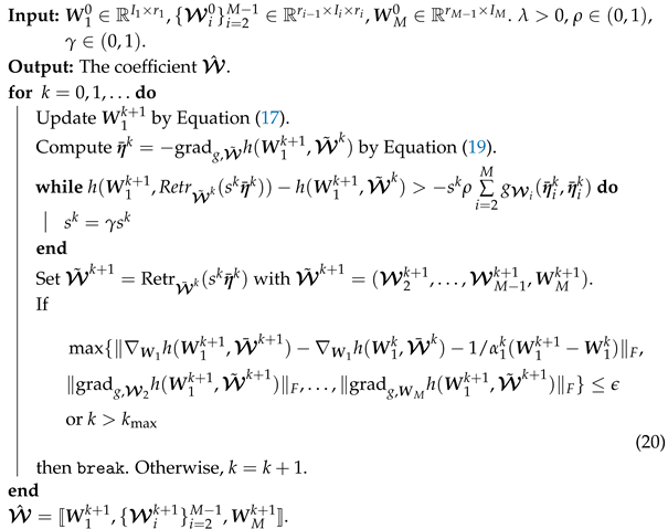
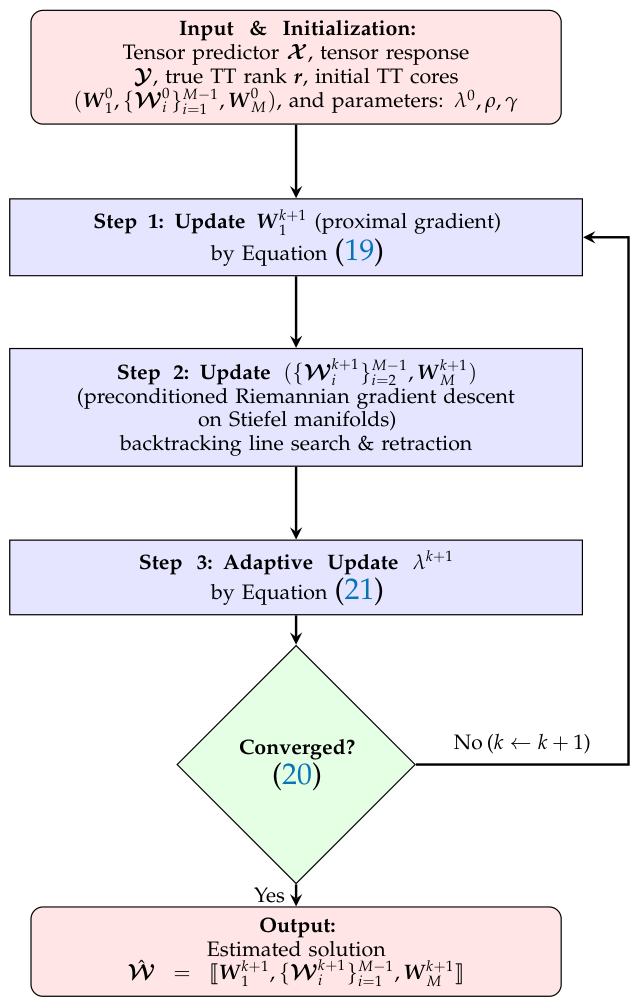
The proposed method, AP2RGD, is outlined in Algorithm 1 (a flowchart is also provided in Figure A1). As we will show in Lemma 1, this backtracking line search procedure is well defined.

Algorithm 1: AP2RGD

At the end of this section, we provide the computational complexity of Algorithm 1, with a focus on evaluating the gradient and Hessian of function h. For the sake of conciseness, let $\overline{I}=\max \{I_i:i\in \left[M\right]\}$ and $\overline{r}=\max \{r_i:i=0,1,\dots ,M\}$. According to Property 1 (i) and (ii), the computational complexity of computing the gradient is

$$\left\{\begin{array}{cc}\mathcal{O}(N{\overline{r}}^2{\overline{I}}^m+N{\overline{r}}^3+{\overline{I}}^{m-i}+{\overline{r}}^4{\overline{I}}^{M-m}),\hfill & \mathrm{if}i\le m,\hfill \\ \mathcal{O}(N{\overline{r}}^2{\overline{I}}^m+N\overline{r}{\overline{I}}^{M-m}+{\overline{r}}^3{\overline{I}}^{M-i}+{\overline{r}}^4{\overline{I}}^{M-i}),\hfill & \mathrm{if}i>m,\hfill \end{array}\right.$$

and the complexity of computing the Hessian is

$$\left\{\begin{array}{cc}\mathcal{O}(N{\overline{r}}^2{\overline{I}}^m+N{\overline{r}}^3{\overline{I}}^{m-i}+N{\overline{r}}^4{\overline{I}}^{M-m}+N{\overline{r}}^3{\overline{I}}^{M-m})\hfill & \mathrm{if}i\le m,\hfill \\ \mathcal{O}(N{\overline{r}}^2{\overline{I}}^m+N{\overline{r}}^2{\overline{I}}^{i-m}+N{\overline{r}}^{M-m+2}{\overline{I}}^{M-m}+N{\overline{r}}^3{\overline{I}}^{M-m}),\hfill & \mathrm{if}i>m,\hfill \end{array}\right.$$

Solving the Lyapunov equation for ${\mathit{S}}_i$ requires a complexity of $\mathcal{O}\left({\overline{r}}^3\right)$.

In summary, the computational complexity per iteration is $\mathcal{O}\left(\max \{N{\overline{r}}^2{\overline{I}}^m+N{\overline{r}}^3{\overline{I}}^{m-i}+N{\overline{r}}^4{\overline{I}}^{M-m},N{\overline{r}}^2{\overline{I}}^m+N{\overline{r}}^{M-m+2}{\overline{I}}^{M-m}+N{\overline{r}}^3{\overline{I}}^{M-m}\}\right).$

4.3. Convergence Analysis

In this section, we establish the convergence of AP2RGD. For notational convenience, let $f({\mathit{W}}_1,\tilde{\mathcal{W}})=h({\mathit{W}}_1,\tilde{\mathcal{W}})+\lambda {\parallel {\mathit{W}}_1\parallel }_{2,0}$.

Lemma 1.

For any given line search parameter, $\rho \in (0,1)$, there exists a constant, $\overline{s}>0$, such that, for any $0<s^k\le \overline{s}$, the backtracking line search procedure is well defined, and the sequence generated satisfies the sufficient decrease condition

$$h({\mathit{W}}_1^{k+1},{\mathit{Retr}}_{{\tilde{\mathit{W}}}^k}\left(s^k{\overline{\eta }}^k\right))-h({\mathit{W}}_1^{k+1},{\tilde{\mathit{W}}}^k)\le -s^k\rho {\displaystyle \sum _{i=2}^M}{g}_{{\mathcal{W}}_i}({\overline{\eta }}_i^k,{\overline{\eta }}_i^k).$$

Theorem 2.

Let ${\left\{({\mathit{W}}_1^k,{\left\{{\mathcal{W}}_i^k\right\}}_{i=2}^{M-1},{\mathit{W}}_M^k)\right\}}_{k\in \mathbb{N}}$ be the sequence generated by Algorithm 1. The following results hold.  

(i) 

The sequence ${\left\{f({\mathit{W}}_1^k,{\left\{{\mathcal{W}}_i^k\right\}}_{i=2}^{M-1},{\mathit{W}}_M^k)\right\}}_{k\in \mathbb{N}}$ is convergent.

(ii) 

The sequence ${\left\{({\mathit{W}}_1^k,{\left\{{\mathcal{W}}_i^k\right\}}_{i=2}^{M-1},{\mathit{W}}_M^k)\right\}}_{k\in \mathbb{N}}$ is bounded.

(iii) 

The sequence ${\left\{({\mathit{W}}_1^k,{\left\{{\mathcal{W}}_i^k\right\}}_{i=2}^{M-1},{\mathit{W}}_M^k)\right\}}_{k\in \mathbb{N}}$ converges to a critical point.

The proofs of Lemma 1 and Theorem 2 are provided in Appendices Appendix F and Appendix G, respectively.

5. Numerical Experiments

All numerical experiments were conducted in MATLAB R2023b on a laptop running on 64-bit Windows with an Intel Core Ultra 9 185H $2.30$ GHz and 32 GB of RAM. We conducted numerical experiments on both simulated and real-world datasets. For the simulated data, we set $ϵ={10}^{-5}\sqrt{I_1}$, whereas for the real-world datasets, we set $ϵ=3\times {10}^{-4}$. Additionally, all methods are terminated once the iteration number reaches the maximum MaxIter $=5\times {10}^3$.

5.1. Synthetic Data

To systematically validate the performance of the proposed framework, the numerical experiments presented in this section evaluate two aspects: algorithmic effectiveness and modeling feasibility.

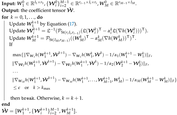
• Example 1. (E1) The effectiveness of the proposed algorithm is verified through a comparison with the first-order algorithm PALM (Algorithm 2).
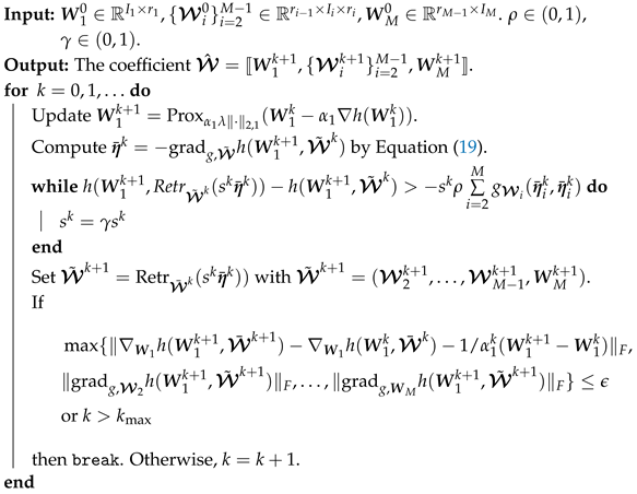
• Example 2. (E2) The effectiveness of the model is validated by comparing the ${\mathcal{l}}_{2,1}$-regularized optimization (22) and the least-squares optimization model (23), which are solved by Algorithm 3 and Algorithm 4, respectively. A total of six simulated datasets are tested in Examples 1 and 2, where we set $m=2$ and $M=4$. The corresponding values for $\mathit{I}$, $\mathit{r}$, and s are detailed in Table 4.

Table 4. Synthetic datasets for E1 and E2.

Datasets	$\mathit{I}=({\mathit{I}}_1,{\mathit{I}}_2,{\mathit{I}}_3,{\mathit{I}}_4)$	$\mathit{r}=({\mathit{r}}_1,{\mathit{r}}_2,{\mathit{r}}_3)$	s
D1	$(20,20,20,20)$	$(2,2,2)$	0.1
D2	$(20,20,20,20)$	$(2,2,2)$	0.2
D3	$(20,20,20,20)$	$(4,4,4)$	0.2
D4	$(30,30,30,30)$	$(2,2,2)$	0.1
D5	$(30,30,30,30)$	$(2,2,2)$	0.2
D6	$(30,30,30,30)$	$(4,4,4)$	0.2

Table 4. Synthetic datasets for E1 and E2.

Datasets	$\mathit{I}=({\mathit{I}}_1,{\mathit{I}}_2,{\mathit{I}}_3,{\mathit{I}}_4)$	$\mathit{r}=({\mathit{r}}_1,{\mathit{r}}_2,{\mathit{r}}_3)$	s
D1	$(20,20,20,20)$	$(2,2,2)$	0.1
D2	$(20,20,20,20)$	$(2,2,2)$	0.2
D3	$(20,20,20,20)$	$(4,4,4)$	0.2
D4	$(30,30,30,30)$	$(2,2,2)$	0.1
D5	$(30,30,30,30)$	$(2,2,2)$	0.2
D6	$(30,30,30,30)$	$(4,4,4)$	0.2

Algorithm 2: PALM

Algorithm 3: AP2RGD (gLasso)

Algorithm 4: AP2RGD (TOD)

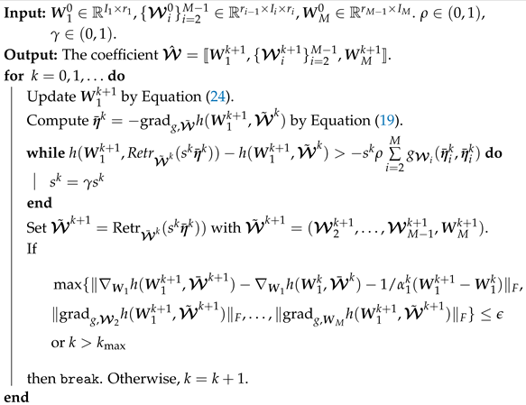Table 4 summarizes the values of $[\mathit{I},\mathit{r},s]$ used in the synthetic datasets for Examples 1 and 2. We construct a synthetic predictor tensor, $\mathcal{X}\in {\mathbb{R}}^{I_1\times \dots I_m\times N}$, where each entry is independently sampled from a Gaussian distribution , $N(0,1/\sqrt{I_1\dots I_m}).$ The ground-truth parameter tensor ${\mathcal{W}}^{\mathrm{R}}=〚{\mathit{W}}_1^{\mathrm{R}},{\mathcal{W}}_2^{\mathrm{R}},\dots ,{\mathit{W}}_M^{\mathrm{R}}〛\in {\mathbb{R}}^{I_1\times \cdots \times I_M}$. The TT-cores ${\mathit{W}}_1^{\mathrm{R}},$ ${\mathcal{W}}_i^R$, $i=2,\dots ,M-1,$ ${\mathit{W}}_M^{\mathrm{R}}$ satisfy $\parallel {\mathit{W}}_1^{\mathrm{R}}{\parallel }_{2,0}=s_0$ and

$$(\mathfrak{L}{\left({\mathcal{W}}_2^R\right)}^{\mathsf{T}},\dots ,\mathfrak{L}{\left({\mathcal{W}}_{M-1}^R\right)}^{\mathsf{T}},{\left({\mathit{W}}_M^R\right)}^{\mathsf{T}})\in \mathrm{St}(I_2{r}_2,r_1)\times \cdots \times \mathrm{St}(I_{M-1}{r}_{M-1},r_{M-2})\times \mathrm{St}(I_M,r_{M-1}).$$

The response tensor $\mathcal{Y}\in {\mathbb{R}}^{I_{m+1}\times \cdots \times I_M\times N}$ is then synthesized by combining the predictor tensor $\mathcal{X}$, the true parameter tensor ${\mathcal{W}}^{\mathrm{R}}$, and an additive noise tensor, where each entry is drawn from a standard Gaussian distribution $\mathcal{N}(0,1)$ and scaled by a factor of 0.001.

To assess the performance of all methods for E1 and E2, we implement the following four metrics: the Relative Estimation Error defined as $\mathrm{REE}=\parallel \widehat{\mathcal{W}}-{\mathcal{W}}^{\mathrm{R}}{\parallel }_F/{\parallel {\mathcal{W}}^{\mathrm{R}}\parallel }_F$, where $\widehat{\mathcal{W}}$ is the approximate estimator generated by each method; the CPU time (s); the total number of iterations (Iter); the row-sparsity $\parallel {\widehat{\mathit{W}}}_1{\parallel }_{2,0}$. Numerical results are reported as the average over 10 independent runs.

Example 1.

To evaluate the algorithmic performance, we compare the proposed AP2RGD method (Algorithm 1) with the PALM algorithm (Algorithm 2). Notably, because the proximal operator of ${\delta }_{\mathit{St}(n,r)}$ is equivalent to the projection onto $\mathit{St}(n,r)$, the ${\mathcal{W}}_i$-subproblem admits a closed-form solution for all $i=2,\dots ,M$, as detailed in Algorithm 2.

Table 5 collects the numerical results of 14 instances with 6 choices of $(\mathit{I},\mathit{r},s)$ with $N=400$ and $N=600$. For each instance, the best results in terms of the aforementioned four metrics are boldfaced, and the estimated $\parallel {\widehat{\mathit{W}}}_1{\parallel }_{2,0}$, which exactly matches that of the ground truth ${\mathit{W}}_1^{\mathrm{R}}$, is also boldfaced. In terms of recovery accuracy, AP2RGD demonstrates exceptional precision. The REE of AP2RGD consistently remains within an extremely low range of 0.003 to 0.009, achieving highly accurate structural recovery. Conversely, PALM exhibits significantly higher REE values, generally ranging from 0.01 to 0.35, indicating a failure to accurately capture the underlying deterministic mapping. The proposed AP2RGD exactly recovers the true number of nonzero components across all parameter combinations. The $\parallel {\widehat{\mathit{W}}}_1{\parallel }_{2,0}$ metric for AP2RGD aligns perfectly with the true nonzero rows. PALM performs poorly in this regard, frequently producing fractional or incorrect sparsity counts and failing to pinpoint the true sparse structure. Table 6 lists the maximum memory consumption (in GB).

Table 5. Average results on synthetic data for E1 with various $\mathit{I}=(I_1,I_2,I_3,I_4)$, $\mathit{r}=(r_1,r_2,r_3)$ and s. nnz$:= \parallel {\mathit{W}}_1^{\mathrm{R}}{\parallel }_{2,0}$. Standard deviations of REE are reported in brackets. Bold font indicates the best results.

Datasets	nnz	REE (AP2RGD$|$PALM)	CPU Time (s) (AP2RGD$|$PALM)	Iter. (AP2RGD$|$PALM)	$\parallel {\widehat{\mathit{W}}}_1{\parallel }_{2,0}$ (AP2RGD$|$PALM)
$N=400$
D1	2	0.0059 (0.0021)$|$0.2764 (0.3149)	16.1274$|$9.5024	300$|$892	2$|$1
D2	4	0.0036 (0.0009)$|$0.2129 (0.3300)	6.0663$|$6.6689	162$|$733	4$|$3
D3	4	0.0053 (0.0008)$|$0.0204 (0.0251)	73.0652$|$42.5561	531$|$2449	4$|$4
D4	3	0.0069 (0.0032)$|$0.3143 (0.3241)	45.8313$|$45.0325	294$|$926	3$|$1.7
D5	6	0.0067 (0.0010)$|$0.0126 (0.0192)	46.3172$|$55.0668	276$|$1140	6$|$6.1
D6	6	0.0099 (0.0022)$|$0.0100 (0.0019)	167.8407$|$78.7146	512$|$1412	6$|$6
$N=600$
D1	2	0.0051 (0.0017)$|$0.2319 (0.2881)	14.6824$|$18.1603	349$|$1431	2$|$1
D2	4	0.0034 (0.0008)$|$0.0043 (0.0006)	29.1847$|$22.2224	167$|$173	4$|$4
D3	4	0.0044 (0.0006)$|$0.0456 (0.0609)	91.8941$|$57.3893	584$|$3217	4$|$4
D4	3	0.0063 (0.0008)$|$0.3543 (0.3684)	40.8414$|$19.3603	261$|$519	2$|$1.5
D5	6	0.0054 (0.0009)$|$0.2257 (0.3581)	30.5841$|$17.9254	195$|$489	4$|$4.2
D6	6	0.0069 (0.0008)$|$0.0167 (0.0211)	74.5372$|$71.6251	366$|$1539	6$|$6

Table 6. Maximum memory consumption (in GB) of the proposed AP2RGD algorithm for E1.

Datasets	N	Max Memory Consumption	N	Max Memory Consumption
D1	400	4.5034 GB	600	4.8624 GB
D2	400	4.5036 GB	600	4.8628 GB
D3	400	4.5053 GB	600	4.8930 GB
D4	400	4.5330 GB	600	4.7913 GB
D5	400	4.5360 GB	600	4.8571 GB
D6	400	4.5343 GB	600	4.9032 GB

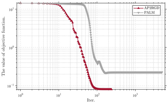
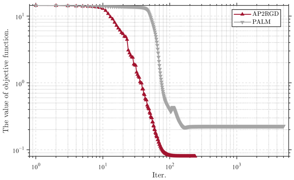
Furthermore, AP2RGD exhibits highly efficient convergence characteristics. It requires substantially fewer iterations to satisfy the convergence criterion compared to PALM, often reducing the iteration count by factors of approximately 3–4. Figure 3 demonstrates the convergence trajectories of the two methods for solving problem (2). Clearly, the AP2RGD method converges much faster than PALM. Although CPU times vary, depending on specific dimension configurations, AP2RGD remains highly competitive and generally more computationally efficient. This comprehensive advantage is especially pronounced, given its superior recovery accuracy.

Figure 3. Convergence behavior of AP2RGD and PALM for E1.

In our implementation, the regularization parameter $\lambda$ is dynamically tuned using the adaptive formulation

$${\lambda }^{k+1}=\min \{{\tau }_1{\lambda }_{\max },{\tau }_2{\lambda }^k\},$$

(21)

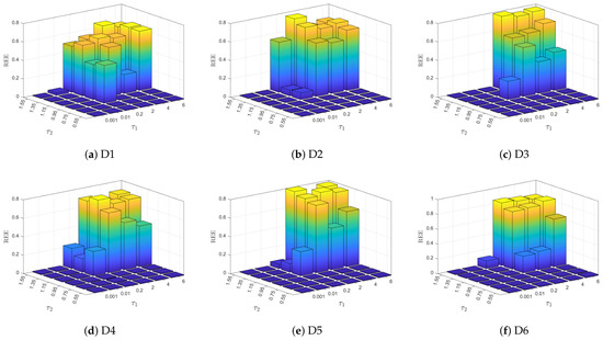
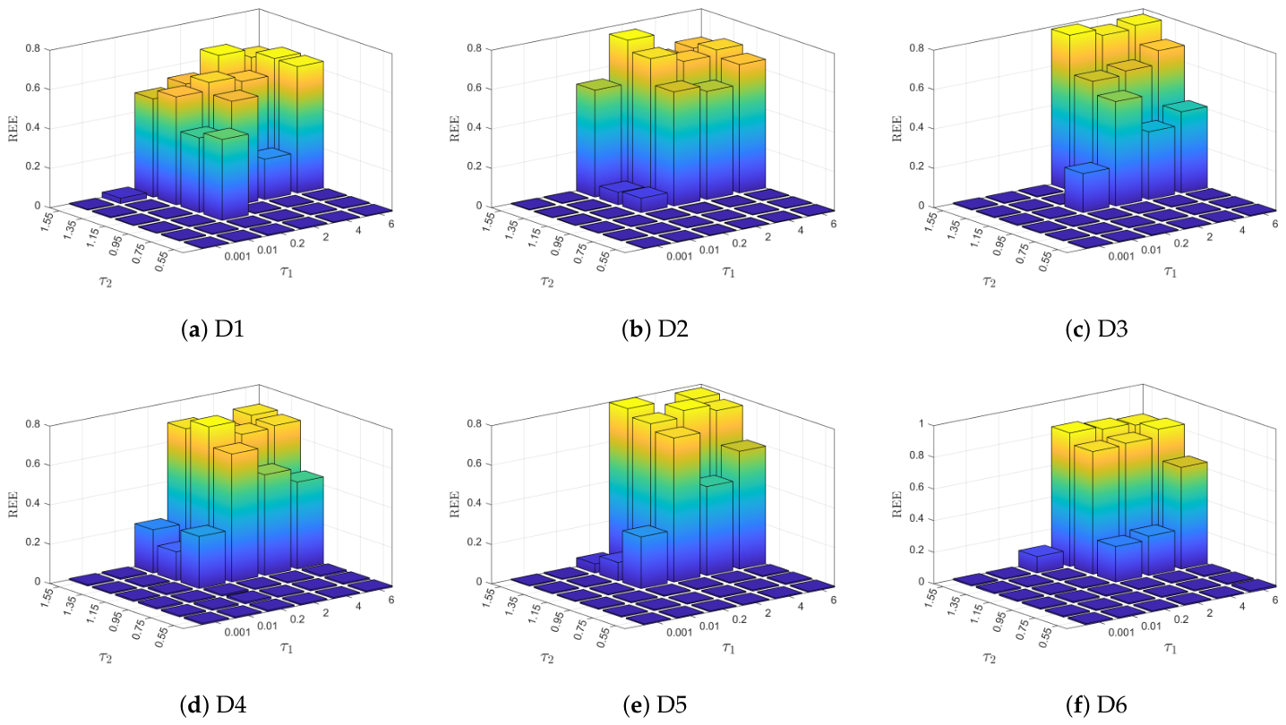
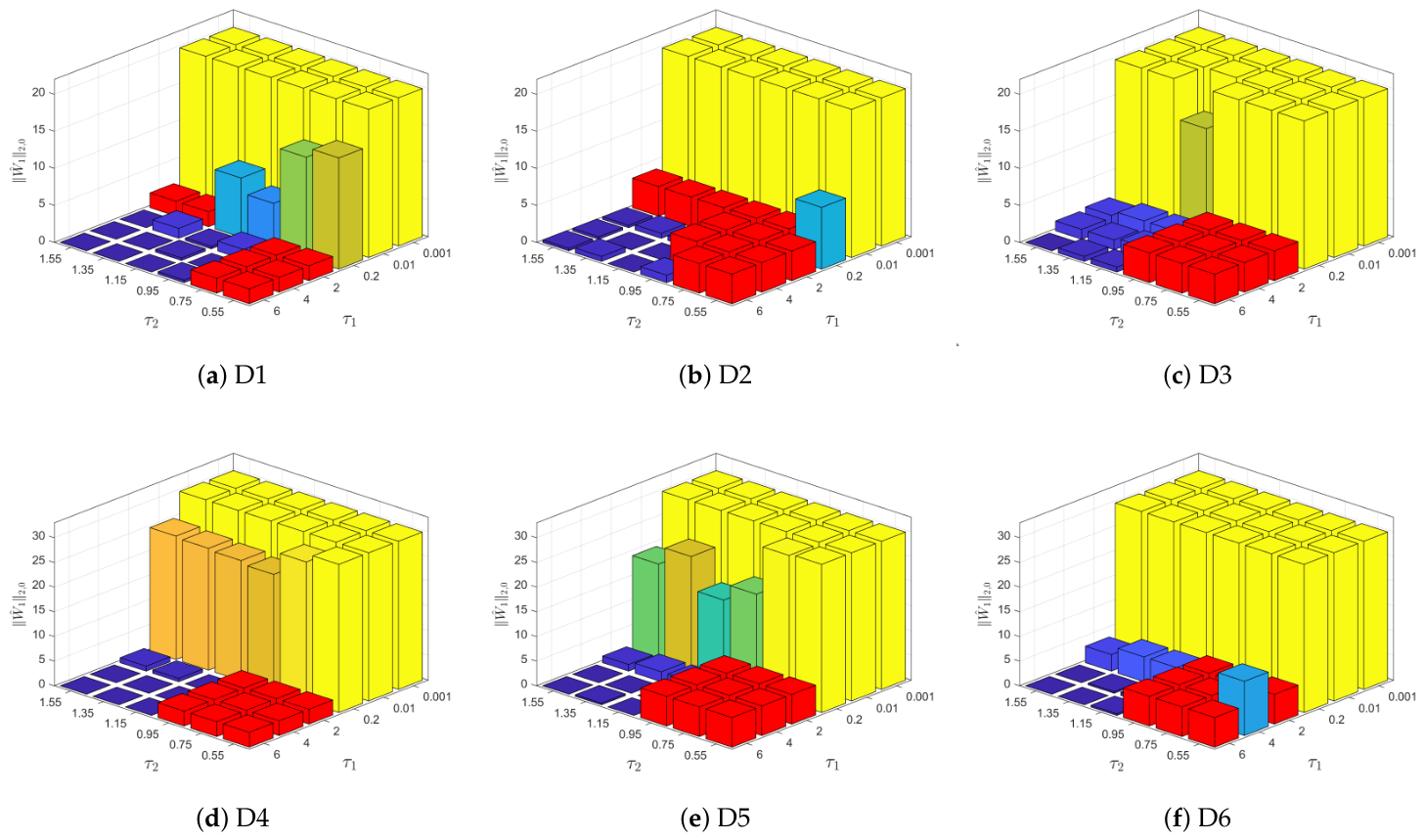
starting with an initial value of ${\lambda }^0=0.1{\lambda }_{\max }$ and ${\lambda }_{\max }=\max \left\{\right|a_{i_1,i_2,\dots ,i_M}|:\mathcal{A}=\mathcal{X}{\times }_{m+1}^{M-m+1}\mathcal{Y}\}$. To evaluate the parameter sensitivity, Figure 4 and Figure 5 plot the average REE and $\parallel {\widehat{\mathit{W}}}_1{\parallel }_{2,0}$ derived from 10 independent trials under different configurations of ${\tau }_1$ and ${\tau }_2$. As observed in Figure 4, when ${\tau }_1\in \{2,4,6\}$ and ${\tau }_2\in \{0.55,0.75\}$, AP2RGD achieves a relatively small REE while ensuring that $\parallel {\widehat{\mathit{W}}}_1{\parallel }_{2,0}=\parallel {\mathit{W}}_1^{\mathbf{R}}{\parallel }_{2,0}$. In contrast, when ${\tau }_1\in \{0.01,0.001\}$, the REE remains relatively small for any ${\tau }_2\in \{0.55,0.75,0.95,1.15,1.35,1.55\}$. Figure 5 indicates that the corresponding values of $\parallel {\widehat{\mathit{W}}}_1{\parallel }_{2,0}$ are quite large, implying a failure to correctly identify the non-zero rows of the ground-truth solution ${\mathit{W}}_1^{\mathbf{R}}$. These findings provide valuable guidance for parameter selection in our numerical experiments.

Figure 4. Effects of ${\tau }_1$ and ${\tau }_2$ on REE across different datasets for E1 when $N=600$. Subplots (a–f) denote the results evaluated on datasets D1–D6, respectively.

Figure 5. Effects of ${\tau }_1$ and ${\tau }_2$ on $\parallel {\widehat{\mathit{W}}}_1{\parallel }_{2,0}$ across different datasets for E1 when $N=600$. Subplots (a–f) denote the results evaluated on datasets D1–D6, respectively. The height of the red bar corresponds to the true number of non-zero rows in $W_1$, which is $\parallel {\mathit{W}}_1^{\mathrm{R}}{\parallel }_{2,0}$.

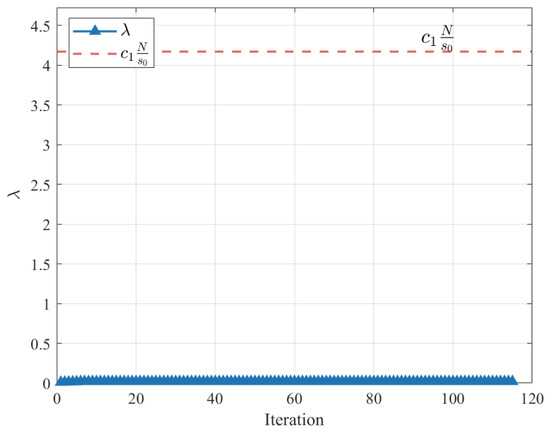
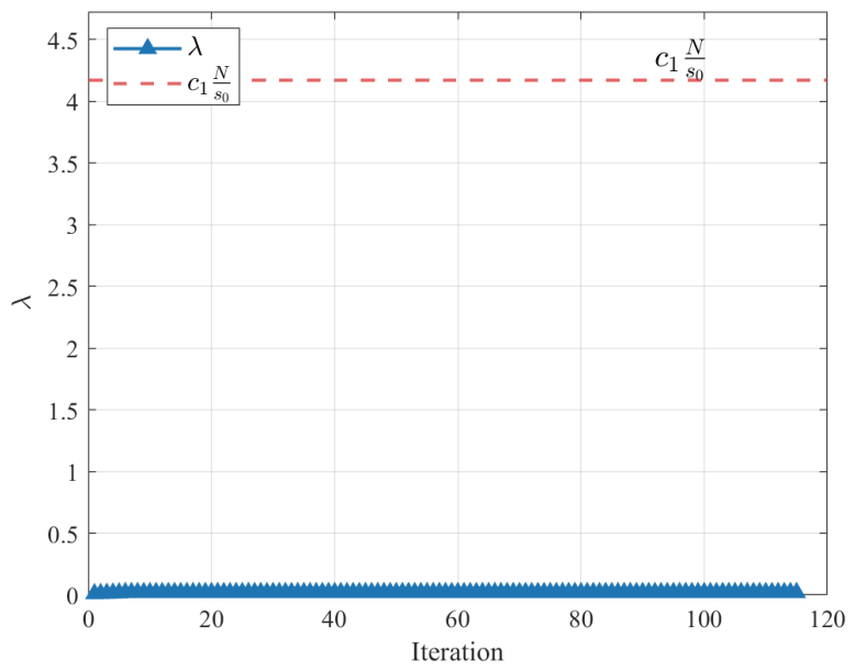
Figure 6 illustrates the evolution of $\lambda$ over iterations, where the red dashed line represents $c_1{\displaystyle \frac{N}{s_0}}$, where $c_1=1/24,$ $N=600,$ and $s_0=6$. As clearly shown, the parameter $\lambda$ consistently satisfies the condition established in Theorem 1.

Figure 6. Evolution of the parameter $\lambda$ over iterations. $c_1=1/24,$ $N=600,$ $s_0=6$.

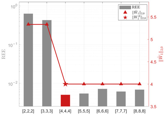
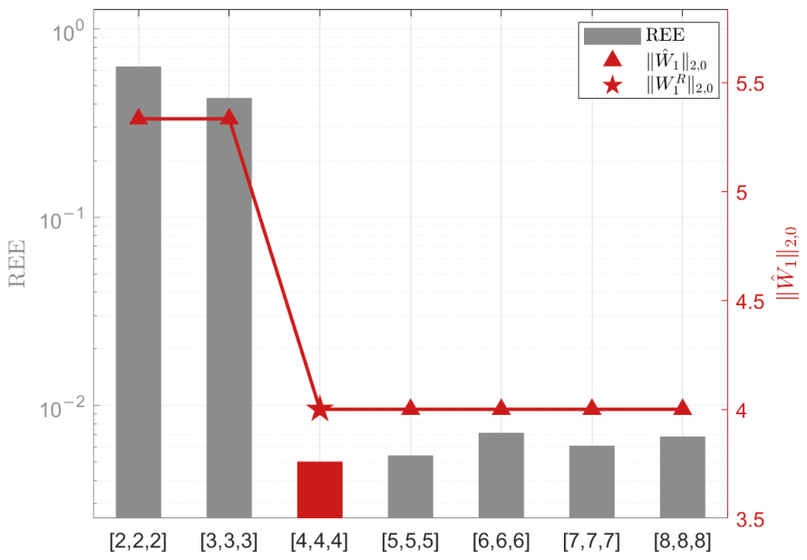
Taking the setting $\mathit{I}=[20,20,20,20]$, $\mathit{r}=[4,4,4]$, and $s=0.2$ as an example, Figure 7 illustrates the corresponding values of REE and $\parallel {\widehat{\mathit{W}}}_1{\parallel }_{2,0}$ when the components of the input rank uniformly decrease or increase. As can be observed from the results, when the rank value is smaller than the true rank (e.g., $[2,2,2]$ and $[3,3,3]$), the REE values are significantly larger. In this case, the estimated $\parallel {\widehat{\mathit{W}}}_1{\parallel }_{2,0}$ deviates from the ground truth, indicating a failure to correctly identify the non-zero rows of ${\mathit{W}}_1^{\mathrm{R}}$. Conversely, when the rank value is equal to or larger than the true rank (i.e., from $[4,4,4]$ to $[8,8,8]$), the REE sharply decreases to a relatively low level and remains stable. Simultaneously, the estimated $\parallel {\widehat{\mathit{W}}}_1{\parallel }_{2,0}$ exactly matches the true value $\parallel {\mathit{W}}_1^{\mathrm{R}}{\parallel }_{2,0}$ (as indicated by the alignment of the red triangles with the red star). This demonstrates that, while underestimating the rank severely degrades performance, overestimating the rank has a minimal impact on the estimation results.

Figure 7. Impact of different rank settings on the estimation performance for E1. The experiment is conducted with the baseline configuration of $\mathit{I}=[20,20,20,20]$, $\mathit{r}=[4,4,4]$, and $s=0.2$. The horizontal axis represents the varying input values for the rank $\mathit{r}$. The primary axis shows the REE, denoted by the bar charts, where the red bar highlights the result at the ground-truth rank setting. The secondary axis indicates the estimated number of non-zero rows, $\parallel {\widehat{\mathit{W}}}_1{\parallel }_{2,0}$, plotted as triangle markers. The red star marker corresponds to the ground-truth value, $\parallel {\mathit{W}}_1^{\mathbf{R}}{\parallel }_{2,0}$.

Example 2.

To demonstrate the effectiveness of the proposed model, we compare the primary formulation (2) against the ${\mathcal{l}}_{2,1}$-regularized optimization (22) and the optimization (23), which omits the ${\mathcal{l}}_{2,0}$-regularized term.

STODgLasso. The STODgLasso framework formulates an optimization problem that minimizes a least-squares data-fitting loss plus an ${\mathcal{l}}_{2,1}$ penalty, subject to Stiefel-manifold constraints.

$$\begin{array}{cc}\hfill \underset{{\left\{{\mathcal{W}}_i\right\}}_{i=1}^M}{\min }& {\displaystyle \frac{1}{2}}\parallel \mathcal{Y}-〚{\mathit{W}}_1,{\left\{{\mathcal{W}}_i\right\}}_{i=2}^{M-1},{\mathit{W}}_M〛{\times }_{1,2,\dots ,m}^{1,2,\dots ,m}{\mathcal{X}\parallel }_F^2+\lambda {\parallel {\mathit{W}}_1\parallel }_{2,1}\hfill \\ \hfill \mathrm{s}.\mathrm{t}.& (\mathfrak{L}{\left({\mathcal{W}}_2\right)}^{\mathsf{T}},\dots ,\mathfrak{L}{\left({\mathcal{W}}_{M-1}\right)}^{\mathsf{T}},{\mathit{W}}_M^{\mathsf{T}})\hfill \\ \hfill & \in \mathrm{St}(I_2{r}_2,r_1)\times \cdots \times \mathrm{St}(I_{M-1}{r}_{M-1},r_{M-2})\times \mathrm{St}(I_M,r_{M-1}).\hfill \end{array}$$

(22)

The subproblem for ${\mathit{W}}_1$ can be solved using the proximal operator of the ${\mathcal{l}}_{2,1}$-norm, while the solution methods for the remaining variables are identical to those in AP2RGD; see Algorithm 3.

TOD. This framework presents an optimization model that minimizes a least-squares data-fitting objective under Stiefel manifold constraints without any sparse regularization.

$$\begin{array}{cc}\hfill \underset{{\left\{{\mathcal{W}}_i\right\}}_{i=1}^M}{\min }& {\displaystyle \frac{1}{2}}\parallel \mathcal{Y}-〚{\mathit{W}}_1,{\left\{{\mathcal{W}}_i\right\}}_{i=2}^{M-1},{\mathit{W}}_M〛{\times }_{1,2,\dots ,m}^{1,2,\dots ,m}\mathcal{X}{\parallel }_F^2\hfill \\ \hfill \mathrm{s}.\mathrm{t}.& (\mathfrak{L}{\left({\mathcal{W}}_2\right)}^{\mathsf{T}},\dots ,\mathfrak{L}{\left({\mathcal{W}}_{M-1}\right)}^{\mathsf{T}},{\mathit{W}}_M^{\mathsf{T}})\hfill \\ \hfill & \in \mathrm{St}(I_2{r}_2,r_1)\times \cdots \times \mathrm{St}(I_{M-1}{r}_{M-1},r_{M-2})\times \mathrm{St}(I_M,r_{M-1}).\hfill \end{array}$$

(23)

The solution to ${\mathit{W}}_1$-subproblem is defined as follows

$${\mathit{W}}_1^{k+1}={\mathrm{vec}}^{-1}\left(\mathrm{vec}\left(\mathcal{Y}{\times }_{1,2,\dots ,M-m,M-m+1}^{M-m+2,M-m+1,\dots ,3,1}{\check{\mathcal{W}}}_{\ge 2}\right)\begin{array}{c}\hfill {\check{\mathcal{W}}}_{⟨2⟩}^{†}\end{array}\right),$$

(24)

where

$${\check{\mathcal{W}}}_{\ge 2}={\mathcal{T}}_{[M-m+3,\dots ,1]}\left({\overline{\mathcal{W}}}_{\ge 2}\right),{\overline{\mathcal{W}}}_{\ge 2}={\mathcal{W}}_{\ge 2}{\times }_{2,\dots ,m}^{2,\dots ,m}\mathcal{X}$$

and

$$\check{\mathcal{W}}={\mathcal{T}}_{[2,1,3,4]}\left(\overline{\mathcal{W}}\right),\overline{\mathcal{W}}={\overline{\mathcal{W}}}_{\ge 2}{\times }_{2,3,\dots ,M-m+1,M-m+3}^{M-m+2,M-m+1,\dots ,3,1}{\check{\mathcal{W}}}_{\ge 2},$$

and † is the Moore-Penrose pseudoinverse. The remaining variables are updated using the same approach as in AP2RGD, and the details of this method are shown in Algorithm 4.

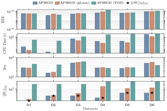
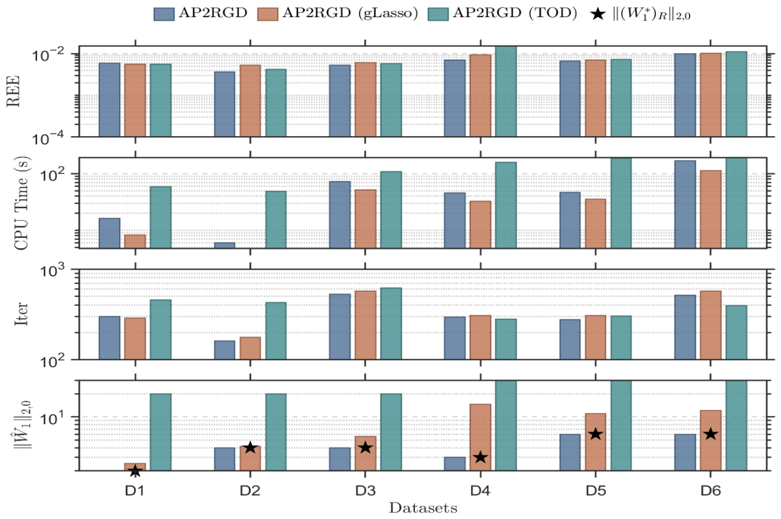
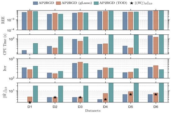
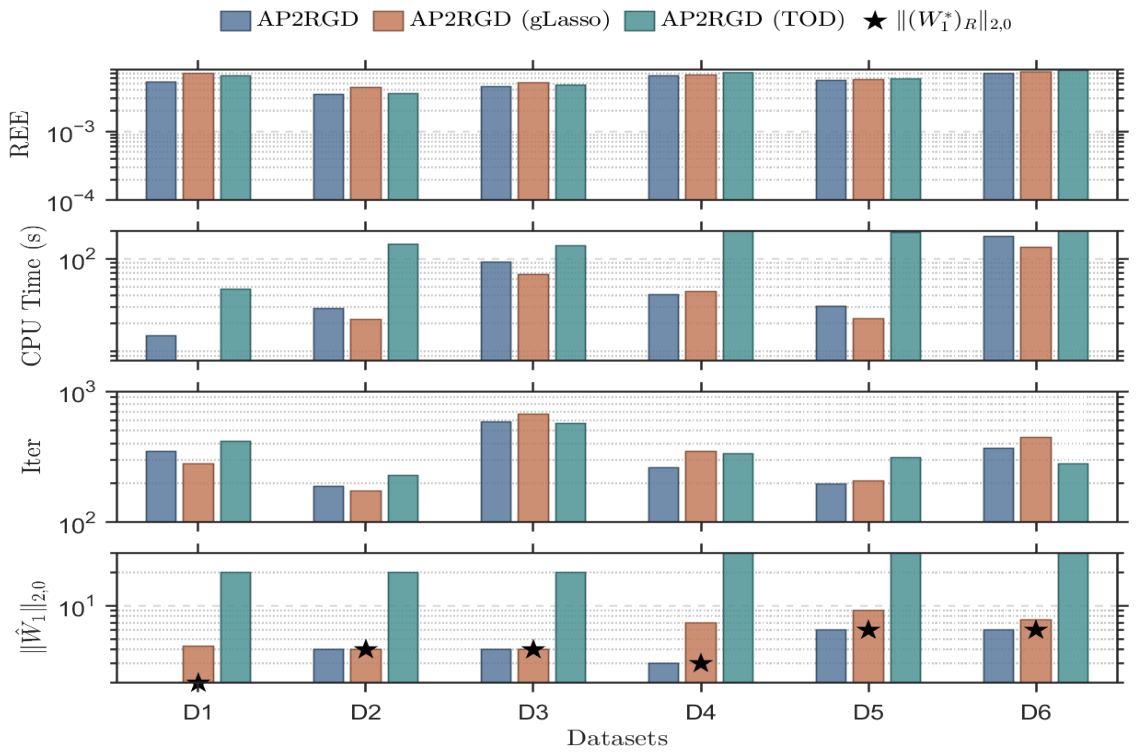
Figure 8 and Figure 9 present the ablation study to comprehensively compare the performance of the proposed method, the variant with ${\mathcal{l}}_{2,1}$ norm regularization, and the baseline model without any regularization terms across six simulation settings (D1 to D6). In terms of REE, all three methods achieve similarly low REE across all datasets. This indicates that the foundational deterministic model effectively reconstructs the target mapping. Although all three methods can attain a low reconstruction error, the main distinction is their ability to recover the true nonzero-row support of ${\mathit{W}}_1$, the core challenge lies in precisely isolating the true nonzero components, rather than merely minimizing the numerical reconstruction error. The three methods exhibit significant differences in the critical task of sparse structure identification. The $\parallel {\widehat{\mathit{W}}}_1{\parallel }_{2,0}$ metric comparison in the figure clearly demonstrates that AP2RGD successfully and exactly identifies the true number of nonzero rows in all datasets, aligning perfectly with the true values marked by black stars. In contrast, AP2RGD (gLasso) fails to recover the correct nonzero-row support in some cases; it significantly overestimates the number of nonzero components, particularly on datasets with more complex parameter scaling (such as D4 to D6). Lacking any regularization term, AP2RGD (TOD) completely loses the ability to select features, resulting in a fully dense solution. Regarding computational efficiency, AP2RGD (TOD) incurs the highest computational cost, requiring significantly more iterations and CPU time than the other two methods. Although the proximal update in AP2RGD (gLasso) is slightly less expensive in a single update step, leading to the shortest total elapsed time, the overall iteration count of AP2RGD is comparable to it. Given the decisive advantage of AP2RGD in accurately pinpointing the true sparse pattern, this modest computational-time trade-off is entirely reasonable and necessary.

Figure 8. Performance comparison of AP2RGD, AP2RGD (gLasso), and AP2RGD (TOD) for E2. $M=4$, $m=2$, $N=400$. The four subplots (from top to bottom) present the REE, CPU time (s), iterations, and estimated non-zero rows ($\parallel {\widehat{\mathit{W}}}_1{\parallel }_{2,0}$) on a logarithmic scale across six datasets (D1–D6). The black star (★) denotes the ground-truth value $\parallel {\left({\mathit{W}}_1^{*}\right)}_R{\parallel }_{2,0}$.

Figure 9. Performance comparison of AP2RGD, AP2RGD (gLasso), and AP2RGD (TOD) for E2. $M=4$, $m=2$, $N=600$. The four subplots (from top to bottom) present the REE, CPU time (s), iterations, and estimated non-zero rows ($\parallel {\widehat{\mathit{W}}}_1{\parallel }_{2,0}$) on a logarithmic scale across six datasets (D1–D6). The black star (★) denotes the ground-truth value $\parallel {\left({\mathit{W}}_1^{*}\right)}_R{\parallel }_{2,0}$.

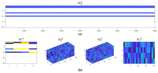
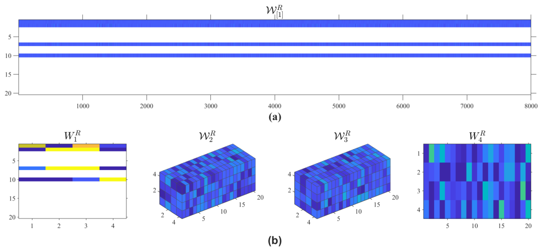
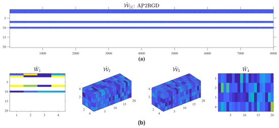
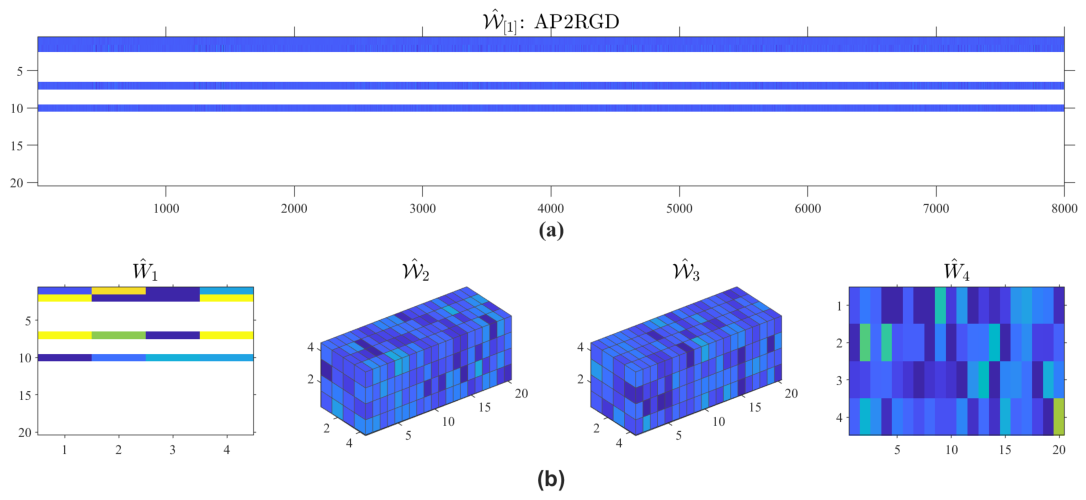
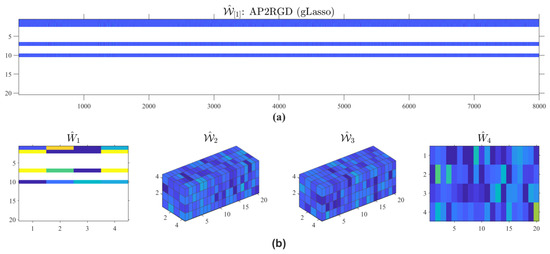
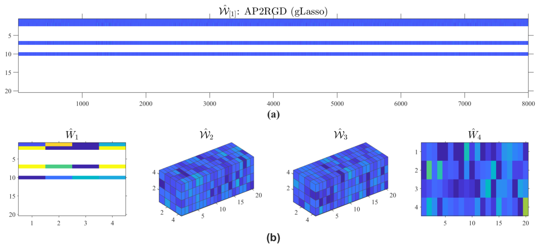
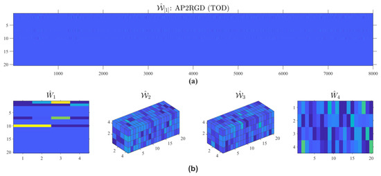
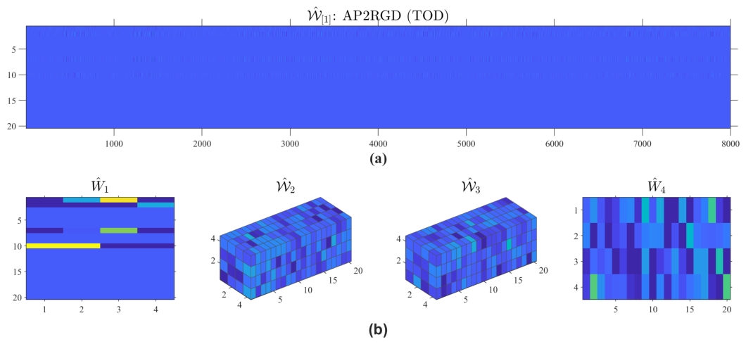
Figure 10, Figure 11, Figure 12 and Figure 13 show the mode-1 unfoldings and TT-core heatmaps for the ground truth and the solutions obtained using AP2RGD, AP2RGD (gLasso), and AP2RGD (TOD), respectively. The parameters for this numerical example are $[\mathit{I},\mathit{r},s]=\left[\right(20,20,20,20),(2,2,2),0.2]$ and $N=400$. As shown in figures, the optimal solution ${\widehat{\mathit{W}}}_1$ obtained using AP2RGD satisfies the equality $\parallel {\widehat{\mathit{W}}}_1{\parallel }_{2,0}=\parallel {\mathit{W}}_1^{\mathrm{R}}{\parallel }_{2,0}={\parallel {\mathcal{W}}^{\mathrm{R}}\parallel }_{m_1,0}=4$, which is consistent with Theorem 1. The proposed method also identifies the locations of the nonzero rows of ${\mathit{W}}_1^{\mathrm{R}}$. Furthermore, the indices of the nonzero rows of its mode-1 unfolding correspond exactly to nonzero-row indices of ${\mathcal{W}}_{\left[1\right]}^{\mathrm{R}}$. This confirms the equivalence between the row-sparsity of ${\mathit{W}}_1$ and the mode-1 hyperslice sparsity of the high-order tensor $\mathcal{W}$. Additionally, the ${\mathcal{l}}_{2,1}$-regularization term in the optimization model (22), acting as a convex relaxation strategy for the ${\mathcal{l}}_{2,0}$-norm, also successfully pinpoints the nonzero rows in ${\widehat{\mathit{W}}}_1$ for this example. Conversely, the estimator obtained from model (23) does not have the ability to identify these nonzero row indices. This indicates a lack of feature selection capability, which consequently incurs a greater computational cost; as reflected by the CPU Time (s) reported in Figure 8 and Figure 9, this method demands the highest execution time.

Figure 10. Visualization of the ground-truth ${\mathcal{W}}^{\mathrm{R}}$ (E2). (a) The mode-1 unfolding matrix ${\mathcal{W}}_{\left[1\right]}^{\mathrm{R}}$. (b) The core matrices and tensors ${\mathit{W}}_1^{\mathrm{R}},{\mathcal{W}}_2^{\mathrm{R}},{\mathcal{W}}_3^{\mathrm{R}},\mathrm{and}{\mathcal{W}}_4^{\mathrm{R}}$. The row-sparsity level is $\parallel {\mathcal{W}}^{\mathrm{R}}{\parallel }_{m_1,0}=4$, visually reflected by the four colored rows in (a) and ${\mathcal{W}}_1^{\mathrm{R}}$. The elements of matrices and tensors are zero (white) and nonzero (color).

Figure 11. Visualization of the optimal solution $\widehat{\mathcal{W}}$ via AP2RGD (E2). (a) The mode-1 unfolding matrix ${\widehat{\mathcal{W}}}_{\left[1\right]}$. (b) The core matrices and tensors ${\widehat{\mathit{W}}}_1,{\widehat{\mathcal{W}}}_2,{\widehat{\mathcal{W}}}_3,\mathrm{and}{\widehat{\mathit{W}}}_4$. The row-sparsity level is $\parallel \widehat{\mathcal{W}}{\parallel }_{m_1,0}=4$, visually reflected by the four colored rows in (a) and ${\widehat{\mathcal{W}}}_1$. The elements of matrices and tensors are zero (white) and nonzero (color).

Figure 12. Visualization of the optimal solution $\widehat{\mathcal{W}}$ via AP2RGD (gLasso) (E2). (a) The mode-1 unfolding matrix ${\widehat{\mathcal{W}}}_{\left[1\right]}$. (b) The core matrices and tensors ${\widehat{\mathit{W}}}_1,{\widehat{\mathcal{W}}}_2,{\widehat{\mathcal{W}}}_3,\mathrm{and}{\widehat{\mathit{W}}}_4$. The row-sparsity level is $\parallel \widehat{\mathcal{W}}{\parallel }_{m_1,0}=4$, visually reflected by the four colored rows in (a) and ${\widehat{\mathcal{W}}}_1$. The elements of matrices and tensors are zero (white) and nonzero (color).

Figure 13. Visualization of the optimal solution $\widehat{\mathcal{W}}$ via AP2RGD (TOD) (E2). (a) The mode-1 unfolding matrix ${\widehat{\mathcal{W}}}_{\left[1\right]}$. (b) The core matrices and tensors ${\widehat{\mathit{W}}}_1,{\widehat{\mathcal{W}}}_2,{\widehat{\mathcal{W}}}_3,\mathrm{and}{\widehat{\mathit{W}}}_4$. The row-sparsity level is $\parallel \widehat{\mathcal{W}}{\parallel }_{m_1,0}=4$, visually reflected by the four colored rows in (a) and ${\widehat{\mathcal{W}}}_1$. The elements of matrices and tensors are zero (white) and nonzero (color).

5.2. Traffic Flow Prediction

Example 3.

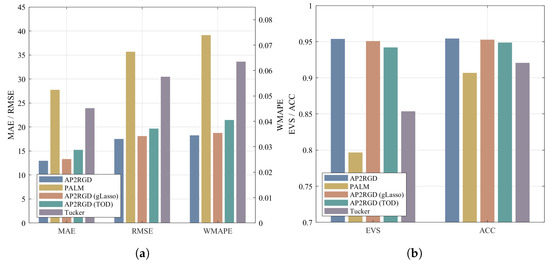
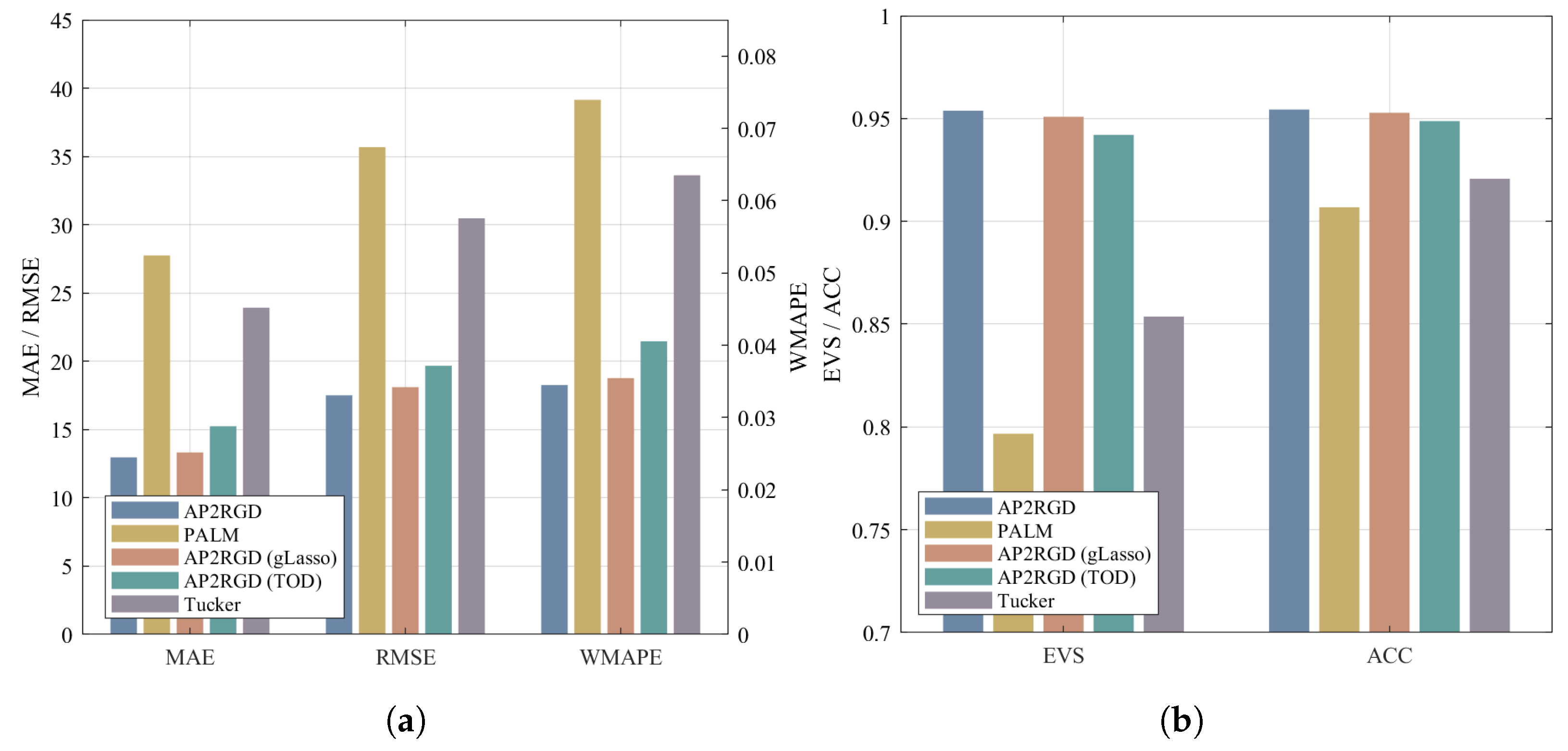
We evaluate the performance of our model by performing spatiotemporal traffic flow prediction on real-world transportation network datasets (https://pems.dot.ca.gov/). In this example, we utilize two days of historical data from 50 traffic zones to forecast the traffic flow of 5 zones across 6 future time steps. Each time step corresponds to a 5-min interval, aggregating to 288 time intervals per day. The dataset comprises a total of 500 samples, and a 5-fold cross-validation approach is employed to select the optimal rank. We compared the three methods (PALM, AP2RGD (gLasso), and AP2RGD (TOD)) mentioned in the simulation data, as well as a sparse tensor-on-tensor regression model based on Tucker decomposition, formulated as:

$$\begin{array}{cc}\hfill \underset{\mathcal{G},{\left\{{\mathit{U}}_i\right\}}_{i=1}^M}{\min }& {\displaystyle \frac{1}{2}}\parallel \mathcal{Y}-〚\mathcal{G};{\mathit{U}}_1,\dots ,{\mathit{U}}_M〛{\times }_{1,2,\dots ,m}^{1,2,\dots ,m}{\mathcal{X}\parallel }_F^2+\lambda {\parallel {\mathit{U}}_1\parallel }_{2,0}\hfill \\ \hfill \mathrm{s}.\mathrm{t}.& ({\mathit{U}}_2,\dots ,{\mathit{U}}_M)\in \mathrm{St}(I_2,r_2)\times \cdots \times \mathrm{St}(I_M,r_M),\hfill \end{array}$$

where $\mathcal{G}\in {\mathbb{R}}^{r_1\times \cdots \times r_M}$ and ${\mathit{U}}_i\in {\mathbb{R}}^{I_i\times r_i},i\in \left[M\right]$ To evaluate algorithmic performance, we define five metrics:

$$\mathit{MAE}={\displaystyle \frac{1}{I_{m+1}\cdots I_M{N}_{\mathit{test}}}}\stackrel{I_{m+1}}{\sum _{i_{m+1}=1}}\cdots \stackrel{I_M}{\sum _{i_M=1}}\stackrel{N_{\mathit{test}}}{\sum _{n=1}}\left|y_{i_{m+1},\cdots ,i_M,n}-{\widehat{y}}_{i_{m+1},\cdots ,i_M,n}\right|,$$

$$\mathit{RMSE}=\sqrt{{\displaystyle \frac{1}{I_{m+1}\cdots I_M{N}_{\mathit{test}}}}\stackrel{I_{m+1}}{\sum _{i_{m+1}=1}}\cdots \stackrel{I_M}{\sum _{i_M=1}}\stackrel{N_{\mathit{test}}}{\sum _{n=1}}{(y_{i_{m+1},\cdots ,i_M,n}-{\widehat{y}}_{i_{m+1},\cdots ,i_M,n})}^2},$$

$$\mathit{WMAPE}=\stackrel{I_{m+1}}{\sum _{i_{m+1}=1}}\cdots \stackrel{I_M}{\sum _{i_M=1}}\stackrel{N_{\mathit{test}}}{\sum _{n=1}}\left({\displaystyle \frac{y_{i_{m+1},\cdots ,i_M,n}}{{\displaystyle \stackrel{I_{m+1}}{\sum _{i_{m+1}=1}}}\cdots {\displaystyle \stackrel{I_M}{\sum _{i_M=1}}}{\displaystyle \stackrel{N_{\mathit{test}}}{\sum _{n=1}}}{y}_{i_{m+1},\cdots ,i_M,n}}}\left|{\displaystyle \frac{y_{i_{m+1},\cdots ,i_M,n}-{\widehat{y}}_{i_{m+1},\cdots ,i_M,n}}{y_{i_{m+1},\cdots ,i_M,n}}}\right|\right),$$

$$\mathit{EVS}=1-{\displaystyle \frac{\mathit{var}(\mathcal{Y}-\widehat{\mathcal{Y}})}{\mathit{var}\left(\mathcal{Y}\right)}},\mathit{and}\mathit{ACC}=1-{\displaystyle \frac{\parallel \mathcal{Y}-\widehat{\mathcal{Y}}{\parallel }_F^2}{{\parallel \mathcal{Y}\parallel }_F^2}}.$$

Here, $N_{\mathit{test}}$ is the number of samples. $\mathcal{Y}$ and $\widehat{\mathcal{Y}}$ represent the ground truth and predicted value, respectively. Lower values for MAE, RMSE, and WMAPE indicate better performance, whereas values closer to 1 are preferable for EVS and ACC. Figure 14 presents the results of these five metrics evaluated across four different methods on this dataset. Across all five evaluation metrics, AP2RGD achieves the lowest values for MAE, RMSE, and WMAPE, alongside the highest values for EVS and ACC. This indicates that the method delivers the best performance on the real-world dataset.

Figure 14. Performance on the real-world dataset for E3. (a) MAE and RMSE on the primary axis, and WMAPE on the secondary axis; (b) EVS and ACC.

Overall, based on the comparison of the numerical results in Section 5.1 and Section 5.2, our method achieves the highest computational accuracy. Particularly on the real-world dataset, it yields the best performance across all predictive metrics. These numerical results demonstrate the effectiveness and feasibility of the proposed model.

6. Conclusions

This paper has proposed an alternating algorithm for a TT-based tensor regression model with sparse regularization and orthogonality constraints. By integrating a preconditioned metric into the subproblems for orthogonal variables, the algorithm achieves improved recovery accuracy. Theoretically, we proved that the algorithm converges to a critical point. Statistically, the variable selection consistency induced by the sparse penalty was established. Finally, numerical experiments on synthetic data and real-world traffic flow dataset verified the feasibility of the proposed model and the practical effectiveness of the algorithm.

References

- Cichocki, A.; Mandic, D.; De Lathauwer, L.; Zhou, G.; Zhao, Q.; Caiafa, C.; Phan, H.A. Tensor Decompositions for Signal Processing Applications: From Two-Way to Multiway Component Analysis. IEEE Signal Process Mag. 2015, 32, 145–163. [Google Scholar] [CrossRef] [Scilit]
- Sidiropoulos, N.D.; De Lathauwer, L.; Fu, X.; Huang, K.; Papalexakis, E.E.; Faloutsos, C. Tensor Decomposition for Signal Processing and Machine Learning. IEEE Trans. Signal Process. 2017, 65, 3551–3582. [Google Scholar] [CrossRef] [Scilit]
- Acar, E.; Yener, B. Unsupervised Multiway Data Analysis: A Literature Survey. IEEE Trans. Knowl. Data Eng. 2009, 21, 6–20. [Google Scholar] [CrossRef] [Scilit]
- Hore, V.; Vinuela, A.; Buil, A.; Knight, J.; McCarthy, M.I.; Small, K.; Marchini, J. Tensor Decomposition for Multiple-Tissue Gene Expression Experiments. Nat. Genet. 2016, 48, 1094–1100. [Google Scholar] [CrossRef] [Scilit]
- Sun, J.; Xiu, X.; Luo, Z.; Liu, W. Learning High-Order Multi-View Representation by New Tensor Canonical Correlation Analysis. IEEE Trans. Circuits Syst. Video Technol. 2023, 33, 5645–5654. [Google Scholar] [CrossRef] [Scilit]
- Sofi, S.S.; De Lathauwer, L. Tensor Train Completion from Fiberwise Observations Along a Single Mode. Mathematics 2026, 14, 922. [Google Scholar] [CrossRef] [Scilit]
- Zhou, H.; Li, L.; Zhu, H. Tensor Regression with Applications in Neuroimaging Data Analysis. J. Am. Stat. Assoc. 2013, 108, 540–552. [Google Scholar] [CrossRef] [Scilit]
- Mu, C.; Huang, B.; Wright, J.; Goldfarb, D. Square Deal: Lower Bounds and Improved Relaxations for Tensor Recovery. In Proceedings of the 31st International Conference on Machine Learning, Bejing, China, 21–26 June 2014; Volume 32, pp. 73–81. [Google Scholar]
- Li, L.; Zhang, X. Parsimonious Tensor Response Regression. J. Am. Stat. Assoc. 2017, 112, 1131–1146. [Google Scholar] [CrossRef] [Scilit]
- Recht, B.; Fazel, M.; Parrilo, P.A. Guaranteed Minimum-Rank Solutions of Linear Matrix Equations via Nuclear Norm Minimization. SIAM Rev. 2010, 52, 471–501. [Google Scholar] [CrossRef] [Scilit]
- Chi, Y.; Lu, Y.M.; Chen, Y. Nonconvex Optimization Meets Low-Rank Matrix Factorization: An Overview. IEEE Trans. Signal Process. 2019, 67, 5239–5269. [Google Scholar] [CrossRef] [Scilit]
- Xiu, X.; Huang, C.; Shang, P.; Liu, W. Bi-Sparse Unsupervised Feature Selection. IEEE Trans. Image Process. 2025, 34, 7407–7421. [Google Scholar] [CrossRef] [Scilit]
- Mao, H.; Dou, J.X. Decomposable Sparse Tensor on Tensor Regression. arXiv 2022, arXiv:2212.05024v2. [Google Scholar]
- Ou-Yang, L.; Zhang, X.F.; Yan, H. Sparse Regularized Low-Rank Tensor Regression with Applications in Genomic Data Analysis. Pattern Recognit. 2020, 107, 107516. [Google Scholar] [CrossRef] [Scilit]
- Oseledets, I.V. Tensor-Train Decomposition. SIAM J. Sci. Comput. 2011, 33, 2295–2317. [Google Scholar] [CrossRef] [Scilit]
- Qin, Z.; Zhu, Z. Computational and Statistical Guarantees for Tensor-on-Tensor Regression with Tensor Train Decomposition. IEEE Trans. Pattern Anal. Mach. Intell. 2025, 47, 10577–10587. [Google Scholar] [CrossRef] [Scilit]
- Gu, Y.; Zhao, P.; Cheng, L.; Guo, Y.; Wang, H.; Ding, W.; Liu, Y. TensorTrack: Tensor Decomposition for Video Object Tracking. Mathematics 2025, 13, 568. [Google Scholar] [CrossRef] [Scilit]
- Oseledets, I.V.; Savostianov, D.V.; Tyrtyshnikov, E.E. Tucker Dimensionality Reduction of Three-Dimensional Arrays in Linear Time. SIAM J. Matrix Anal. Appl. 2008, 30, 939–956. [Google Scholar] [CrossRef] [Scilit]
- Ahmed, T.; Raja, H.; Bajwa, W.U. Tensor Regression Using Low-Rank and Sparse Tucker Decompositions. SIAM J. Math. Data Sci. 2020, 2, 944–966. [Google Scholar] [CrossRef] [Scilit]
- Pan, C.; Ling, C.; He, H.; Qi, L.; Xu, Y. A Low-Rank and Sparse Enhanced Tucker Decomposition Approach for Tensor Completion. Appl. Math. Comput. 2024, 465, 128432. [Google Scholar] [CrossRef] [Scilit]
- Chen, Y.; Luo, Z. Group SLOPE Penalized Low-Rank Tensor Regression. J. Mach. Learn. Res. 2023, 24, 352. [Google Scholar]
- Kokoszka, P.; Reimherr, M. Introduction to Functional Data Analysis; Chapman and Hall/CRC: Boca Raton, FL, USA, 2017. [Google Scholar]
- Fan, Z.; Reimherr, M. High-Dimensional Adaptive Function-on-Scalar Regression. Econom. Stat. 2017, 1, 167–183. [Google Scholar] [CrossRef] [Scilit][Green Version]
- Donoho, D.L.; Elad, M. Optimally Sparse Representation in General (Nonorthogonal) Dictionaries via ℓ1 Minimization. Proc. Natl. Acad. Sci. USA 2003, 100, 2197–2202. [Google Scholar] [CrossRef] [Scilit]
- Hu, Z.; Chen, Z. Proximal Alternating Linearized Minimization Algorithm for Sparse Tensor Train Decomposition. Stat. Optim. Inf. Comput. 2025, 13, 2119–2135. [Google Scholar] [CrossRef] [Scilit]
- Gao, B.; Peng, R.F.; Yuan, Y.X. Optimization on Product Manifolds under a Preconditioned Metric. SIAM J. Matrix Anal. Appl. 2025, 46, 1816–1845. [Google Scholar] [CrossRef] [Scilit]
- Rockafellar, R.T.; Wets, R.J.B. Variational Analysis; Springer: New York, NY, USA, 2009. [Google Scholar]
- Attouch, H.; Bolte, J.; Svaiter, B. Convergence of Descent Methods for Semi-Algebraic and Tame Problems: Proximal Algorithms, Forward-Backward Splitting, and Regularized Gauss-Seidel Methods. Math. Program. 2013, 137, 91–129. [Google Scholar] [CrossRef] [Scilit]
- Shen, X.; Pan, W.; Zhu, Y. Likelihood-Based Selection and Sharp Parameter Estimation. J. Am. Stat. Assoc. 2012, 107, 223–232. [Google Scholar] [CrossRef] [Scilit]
- Chen, Y.; Luo, Z.; Kong, L. ℓ2,0-Norm Based Selection and Estimation for Multivariate Generalized Linear Models. J. Multivar. Anal. 2021, 185, 104782. [Google Scholar] [CrossRef] [Scilit]
- Wong, W.H.; Shen, X.T. Probability Inequalities for Likelihood Ratios and Convergence Rates of Sieve MLES. Ann. Stat. 1995, 23, 339–362. [Google Scholar] [CrossRef] [Scilit]
- Wang, C.; Zhao, X.L.; Zheng, Y.B.; Li, B.Z.; Ng, M.K. Functional Tensor Singular Value Decomposition. SIAM J. Sci. Comput. 2025, 47, A2180–A2204. [Google Scholar] [CrossRef] [Scilit]
- Gao, B.; Peng, R.; Yuan, Y.X. Riemannian Preconditioned Algorithms for Tensor Completion via Tensor Ring Decomposition. Comput. Optim. Appl. 2024, 88, 443–468. [Google Scholar] [CrossRef] [Scilit]
- Boumal, N. An Introduction to Optimization on Smooth Manifolds; Cambridge University Press: Cambridge, UK, 2023. [Google Scholar] [CrossRef] [Scilit]
- Beck, A. First-Order Methods in Optimization; Society for Industrial and Applied Mathematics (SIAM): Philadelphia, PA, USA, 2017. [Google Scholar] [CrossRef] [Scilit]
Disclaimer/Publisher’s Note: The statements, opinions and data contained in all publications are solely those of the individual author(s) and contributor(s) and not of MDPI and/or the editor(s). MDPI and/or the editor(s) disclaim responsibility for any injury to people or property resulting from any ideas, methods, instructions or products referred to in the content. |
© 2026 by the authors. Licensee MDPI, Basel, Switzerland. This article is an open access article distributed under the terms and conditions of the Creative Commons Attribution (CC BY) license.