End-to-End Graph-Embedded Reinforcement Learning for Solving the Shortest Path Problem with Constraints

Abstract

The shortest path problem (SPP) with constraints constitutes a fundamental yet computationally prohibitive NP-hard challenge in operations research and logistics. Traditional optimization algorithms, including both exact and approximate methods, often suffer from prohibitive computational times and severe scalability bottlenecks on large-scale instances. In contrast, emerging Neural Combinatorial Optimization (NCO) approaches offer the potential for rapid inference but frequently fail to guarantee structural feasibility under strict constraints. To bridge this gap, this study introduces E2E_GERL, a novel end-to-end graph-embedded reinforcement learning algorithm for the time-constrained SPP. The problem is reformulated as a structure-aware and resource-aware sequential decision-making process, where a neural graph embedding network, structure2vec, is integrated to capture the long-term structural equivalence of critical graph nodes. In our framework, a ReLU-based Lagrangian penalty is introduced to embed time constraint violation into the learning objective, and n-step Q-learning is employed to effectively overcome delayed path-level consequences. Extensive experiments on synthetic graphs, modified benchmark instances, and a real-world logistics network demonstrate the superiority of the proposed algorithm, E2E_GERL. It achieves better results with substantially lower inference time than classical and NCO baselines, which also validate the potential of integrating NCO into constrained optimization problem algorithms.

1. Introduction

The SPP represents a fundamental optimization challenge with extensive applications in domains such as transportation, logistics, communication networks, and supply chain decision systems. As a combinatorial optimization problem, it is often associated with the NP-hard characteristic, a trait it shares with numerous other complex problems [1]. This NP-hard nature makes finding good solutions for SPPs particularly challenging, especially for large instances. Early research in this area led to the development of two main categories of algorithms: exact algorithms and approximate algorithms [1,2,3,4,5].

Each of these algorithms has its own strengths and weaknesses. Exact algorithms can find precise solutions for smaller-scale problems but often require significant computational time. On the other hand, approximate algorithms trade off accuracy for speed in finding near-optimal solutions. These algorithms are typically applied to specific problems and often require extensive manual tuning through trial and error, which does not guarantee optimization performance. Although traditional algorithms have been instrumental in solving optimization problems, their low efficiency and unsuitability for large instances still limit their effectiveness in many cases.

The rapid advancement of machine learning methods has made scholars increasingly optimistic that these sophisticated tools can be harnessed to design more efficient NCO algorithms. Nowadays, an increasing number of scholars are turning their attention to this direction. Machine learning for combinatorial optimization offers a complementary strategy: rather than solving each instance from the beginning, a model can exploit regularities across a distribution of problem instances and learn reusable construction policies. Some proposed algorithms that utilize machine learning methods can truly achieve better performance than traditional algorithms with even less computational resources [6,7,8,9]. According to Kotary et al. [10], existing research on leveraging machine learning methods for designing new NCO algorithms mainly adopts two structures: augmented and end-to-end.

The augmented structure primarily uses traditional optimization algorithms to solve problems, supplemented by machine learning methods for decision-making, which involves adapting important features of traditional optimization algorithms, such as parameter tuning. In contrast, the end-to-end structure integrates machine learning methods with optimization problems to form a holistic learning model that is trained and improved to directly provide solutions.

The augmented structure enhances the performance of traditional algorithms through machine learning, meaning the overall effectiveness depends heavily on the traditional algorithms. Consequently, some drawbacks of traditional algorithms are also reflected. For instance, it is necessary to select the corresponding benchmark algorithm for specific problems; otherwise, the overall performance is greatly discounted. This makes it challenging for such algorithms to establish a generalized framework, lacking generalization ability. Additionally, due to the modular structure, the combination of different parts can lead to error accumulation. In complex systems, these errors can significantly impact the overall performance [11].

In contrast, the end-to-end architecture simplifies system complexity by treating the whole system as a single module, thereby reducing the likelihood of error accumulation. End-to-end algorithms can directly optimize the overall system from input to output, often achieving better performance. This approach makes them more adaptable to different inputs and environments, thus exhibiting good generalization ability in many cases.

Designing end-to-end algorithms to solve optimization problems has shown great potential, though it is still in its early stage of development. Current research primarily addresses a relatively limited subset of simple optimization problems, such as the classic Traveling Salesman Problems (TSPs) and Vehicle Routing Problems (VRPs), with minimal focus on the SPP, which has unique graph structures. Moreover, most of these algorithms are unable to handle constrained problems, and the challenges posed by parameterized constraints hinder their broader applicability. Therefore, designing an end-to-end algorithm that can effectively solve the SPP with constraints is the primary motivation of this work.

There are two main machine learning methods that can be combined with end-to-end algorithms: supervised learning and reinforcement learning [7,12,13,14,15]. In the two methods, supervised learning requires labeled data for training, which are difficult to obtain in these NP-hard problems. In contrast, reinforcement learning does not rely on optimal labels; instead, it continuously receives feedback rewards through the interaction of an agent with the environment.

Most optimization problems, including the SPP, inherently possess an objective function. The solution process can be viewed as continuously receiving reward feedback from interactions with this objective function, which acts as a reward function in reinforcement learning. Therefore, reinforcement learning demonstrates greater adaptability in integrating our algorithms.

Despite recent progress in NCO, most end-to-end studies have concentrated on TSPs, VRPs, or unconstrained graph problems. The SPP is structurally different because only a source-to-destination path is required, feasible actions are defined by graph adjacency, and the resource constraint must be respected throughout path construction. These differences motivate a learning framework that simultaneously encodes graph structure, partial-solution state, and constraint consumption. This paper aims to design a reinforcement learning-based end-to-end algorithm for solving the SPP with constraints. Two main challenges exist: one arising from the problem structure of the SPP, and the other from the constraints. Researchers have observed that optimization problems within the same category often share a similar problem structure, differing mainly in data [16]. As a classic graph theory problem, different instances of SPPs share the same graph structure [17]. By learning from many instances, the model can approximate a reusable node selection heuristic that exploits these regularities while avoiding the manual feature engineering required by classical heuristics. However, traditional optimization algorithms often fail to exploit this inherent structural similarity effectively.

To bridge these critical methodological gaps, this study introduces a novel end-to-end reinforcement learning framework, designated as E2E_GERL, specifically for the constrained SPP. Rather than treating constraints as rigid roadblocks or relying on myopic heuristics, we reformulate the constrained routing task into a sequential decision-making process. Starting from the origin node, it incrementally constructs a path by selecting feasible successor nodes until the destination node is reached. We integrate a structure2vec graph embedding module to dynamically capture the structural equivalence of network nodes. Based on this representation, an action-value function evaluates the long-term utility of selecting each candidate successor node under the current partial path state. Furthermore, instead of treating the time constraint as an external post-processing condition, we introduce a ReLU-based Lagrangian penalty to embed time constraint violation directly into the reinforcement learning reward. When a generated path satisfies the time constraint, the penalty is inactive and the objective reduces to the original path cost, while when the time constraint is violated, the magnitude of violation is explicitly penalized.

Here are the main contributions of this paper:

• A resource-aware sequential formulation of the time-constrained shortest path problem is proposed. We formulate the time-constrained shortest path problem as a finite-horizon Markov decision process in which the state jointly represents the ordered partial path, current and destination nodes, visited-node status, accumulated routing cost, accumulated travel time, and the prescribed time budget. This formulation captures a defining property of resource-constrained path optimization: two partial paths reaching the same node may have different future feasibility because they consume different amounts of the available resource. The resulting action space is restricted to structurally admissible successor nodes, enabling source-to-destination path construction directly on sparse directed graphs.
• A state-dependent resource-aware graph value model for cumulative resource path decisions is proposed. We develop a graph-based action-value model in which the value of each candidate path extension is conditioned jointly on graph topology, directed edge attributes, the evolving partial path, and cumulative resource consumption. The graph representation is updated as the constrained path state changes, enabling candidate nodes to be evaluated according to their role under the current path and remaining resource context rather than through a static node representation.
• A constraint-aligned reinforcement learning objective with exact path-level return equivalence is proposed. Building on established Lagrangian constraint handling, we define the immediate reward as the negative increment of a ReLU–Lagrangian path objective. With a fixed within-episode multiplier and an undiscounted finite-horizon return γ = 1, we show that the cumulative return of every completed trajectory telescopes exactly to the negative terminal penalized path cost. This establishes an explicit mathematical alignment between sequential value learning and the original constrained path objective.

2. Literature Review

In this section, we discuss the connections between our study and several streams of the literature in terms of the problems, algorithms, and framework.

(1)

Section 2.1: We first demonstrate the classification of traditional algorithms for solving the SPP in previous works and point out their limitations.

(2)

Section 2.2: We review existing end-to-end NCO algorithms that perform well on some combinatorial optimization problems and analyze why end-to-end algorithms are seldom designed for the SPP and constrained problems.

(3)

Section 2.3: We discuss the constraint handling approaches in recent NCO and safe RL with our proposed method.

(4)

Section 2.4: We collate and analyze common graph embedding networks and select the structure2vec network for our work.

2.1. Traditional Algorithms for the Shortest Path Problem

The SPP is a typical problem in both combinatorial optimization and graph theory, with widespread applications. Consequently, research into algorithms for solving the SPP has remained a hot topic [1,5,18,19]. Traditional algorithms for solving the SPP have indeed achieved good results to some extent. These algorithms can generally be categorized into several types: path sorting, dynamic programming, labeling methods, and relaxation methods. They can be either exact or approximate, and the choice of algorithm depends on the graph’s characteristics and the application’s requirements.

In Chitra & Subbaraj [20], the authors used an elitist multi-objective evolutionary algorithm to solve the dynamic SPP in computer networks which is based on the non-dominated sorting genetic algorithm (NSGA). Their results for a sample test network demonstrated the proposed approach’s capabilities to generate well-distributed Pareto-optimal solutions for dynamic routing problems in a single run. Another study proposed a dynamic programming algorithm to solve a variant of the SPP, the k-Color SPP (k-CSPP). The numerical validation results showed that the dynamic programming algorithm vastly outperformed previous approaches [21]. Wang, Yang, and Gao [22] investigated a constrained SPP that makes assumptions on the link travel time in a transportation network, treating it as a random variable defined by a joint probability mass function. The constraints in this problem encompass common traffic balance and side constraints, along with a unique link selection constraint. The proposed algorithm is based on the 0–1 integer programming model, combined with the Lagrangian relaxation method to handle the constraints, decomposing the hard constraint relaxation into two parts. Duque, Lozano, and Medaglia [23] designed an exact algorithm for the bi-objective shortest path problem (BSP) that uses implicit enumeration to recursively prune the dominant solutions and ultimately obtain an exact solution. Irnich and Desaulniers [24] present a comprehensive taxonomy of constrained shortest path problems and conduct a survey of established solution methodologies. The review primarily focuses on algorithms grounded in dynamic programming, Lagrangian relaxation, and constraint programming techniques.

Recent research demonstrates that exact and approximate algorithms for resource-constrained shortest paths continue to advance. Jin and Yu [25] developed a two-stage exact method for doubly resource-constrained elementary shortest paths, combining resource-based network reduction with an improved pulse search. Ahmadi et al. [26] proposed an enhanced bidirectional A* framework for a resource-constrained shortest path (RCSP) problem in large networks, using constraint-aware pruning to substantially reduce search effort. These developments show that modern methods increasingly rely on stronger bounds, state-space reduction, dominance, and heuristic-guided bidirectional search rather than conventional one-directional labeling alone.

Nevertheless, these traditional algorithms still solve each instance through explicit combinatorial search and may face increasing computational effort as instance size, resource dimensionality, or constraint difficulty grows. This motivates the exploration of new methods for improvement. Learning-based methods with an end-to-end structure offer a promising avenue for this purpose.

2.2. End-to-End NCO Algorithms for Combinatorial Problems

With the rapid development of machine learning technologies, many relevant problems have become trends in their respective fields, and the optimization domain is no exception [13,27,28,29,30,31,32,33]. Many studies have adopted the end-to-end algorithmic structure to build NCO frameworks for solving optimization problems [34,35,36,37,38].

To address the TSP problem, Bello et al. [39] designed a framework that leverages machine learning methods. Within this framework, they utilized reinforcement learning to train a recurrent neural network capable of predicting the arrangement of different cities. Another study incorporated the optimization problem’s structure into the framework, representing the structures through graphs, and proposed a unique combination of reinforcement learning and graph embedding to solve them [16]. They demonstrated that their framework could be applied to some optimization problems over graphs, such as Minimum Vertex Cover, Maximum Cut, and TSPs, which have no constraints. However, their framework could not solve the SPP and optimization problems with constraints.

Surprisingly, existing end-to-end algorithms have not focused on the SPP. Most of them are primarily designed to solve optimization problems such as TSPs [34,39,40,41] and VRPs [6,8,42,43,44,45]. For example, Pointer network [46] and attention-based solvers [47] learn constructive policies for TSPs and VRPs, but their canonical formulations assume complete graphs or problem-specific decoder structures and do not directly address source-to-destination constrained shortest paths. Graph embedding RL frameworks [16] learn greedy policies over graphs but have mainly targeted unconstrained graph problems or TSP-like objectives. In these problems, there is usually only one edge considered between any two nodes, and solutions are paths where the starting and ending nodes always coincide, requiring traversal of all nodes.

In contrast, the SPP is different as it can have many different edges between any two nodes, and the ending node is distinct and needs to be identified. Additionally, end-to-end algorithms typically handle simplified optimization problems without constraints, making them less applicable to constrained SPPs. This is primarily because incorporating constraints into a holistic learning model for training and solving in an end-to-end structure is highly challenging. As a result, the existing literature often simplifies optimization problems, ignoring constraints and focusing solely on the objective function when using end-to-end structures.

In this work, we design an end-to-end algorithm combining machine learning methods to solve the SPP. Existing research mainly combines machine learning methods through two approaches: supervised learning [48] and reinforcement learning [49,50]. Each of these machine learning methods has its own characteristics. Although supervised learning methods are currently the most well known and successful within machine learning, their reliance on labeled data renders them less suitable for the SPP. The primary obstacle lies in the fact that these problems are often NP-hard, making it challenging to obtain optimal labels for training supervised learning models [7].

Upon realizing the limitations of supervised learning, attention shifted towards reinforcement learning. Reinforcement learning differs significantly from supervised learning as it does not heavily depend on optimal labels from data. Instead, it interacts with an environment to continually receive feedback, ultimately maximizing cumulative rewards during training [51]. The SPP inherently possesses an objective function, which can be viewed as a reward function in reinforcement learning. By continuously comparing the quality of solutions, rewards can be obtained, aligning well with the principles of reinforcement learning.

Considering the characteristics of the SPP, its NP-hard nature makes it difficult to obtain labeled data. Meanwhile, the nature of path optimization problems naturally fits the framework of reinforcement learning. Therefore, the algorithm design in this study combines reinforcement learning methods. The model characteristics of the SPP make it highly suitable for reinforcement learning. Additionally, as a classic problem in graph theory, its graph structure offers many interesting points worth delving into.

2.3. Constraint Handling in NCO and Safe RL

Constraint handling has always been an important topic in NCO. Earlier works incorporate Lagrangian relaxation and constrained policy optimization into neural routing for constrained TSPs and VRPs, demonstrating that neural policies can explicitly trade solution quality against constraint violation. More recently constrained combinatorial optimization approaches have moved beyond conventional feasibility masking. Bi et al. [52] proposed Proactive Infeasibility Prevention (PIP), which incorporates Lagrangian-based constraint awareness and preventative masking for routing constraints. Recent approaches further combine learned construction with lazy feasibility masking and backtracking to improve feasibility under difficult routing constraints [53,54]. A related research stream is safe reinforcement learning, where cumulative trajectory costs are typically modeled through constrained Markov decision processes. Wu et al. [55] has shown that inaccurate cumulative cost estimation can substantially affect constraint satisfaction, particularly in off-policy learning. Alternative formulations augment the state with cumulative constraint information and apply reward penalties to infeasible trajectories. Finite-horizon safe RL studies have further highlighted the importance of treating non-discounted trajectory constraints explicitly rather than relying on infinite-horizon discounted approximations [56].

These researches demonstrate that Lagrangian relaxation, primal–dual optimization, cumulative cost state augmentation, reward penalization, and feasibility-aware decoding are established techniques for constrained learning. E2E_GERL specializes constraint-aware reinforcement learning to the time-constrained shortest path setting, where the decision process constructs only a source-to-destination path on a sparse directed graph and must condition each action on the evolving partial path and accumulated resource consumption. In particular, the contribution of the proposed constraint formulation lies in defining the instantaneous reward as the negative increment of the ReLU–Lagrangian path objective. Under the finite-horizon undiscounted setting γ = 1, the cumulative return of a completed trajectory telescopes exactly to the negative terminal penalized path cost. This provides an explicit alignment between sequential value learning and the SPP with time constraints and the path-level objective, rather than introducing Lagrangian relaxation itself as a new constrained optimization principle.

2.4. Graph Embedding Networks

The SPP is a classic graph theory problem and fully leveraging its structural features presents a challenge. One promising approach is to solve it using graph embedding techniques. These techniques can be very useful tools [37,38,57]. As a dimensionality reduction method, graph embedding aims to represent nodes on a graph as vectors in a low-dimensional space [58]. In this low-dimensional space, the node information and topological structure of the original graph network are preserved, making vector space operations simpler and faster than graph operations. Moreover, it allows for the direct application of existing machine learning algorithms. Essentially, the core of graph embedding methods is to transform attributed graphs into vector representations by finding low-dimensional representations of high-dimensional graphs, followed by applying machine learning methods to accomplish subsequent tasks.

Graph embedding methods preserve different notions of similarity and should therefore be distinguished according to the structural information they are designed to encode. Random walk approaches such as Node2Vec [59] and DeepWalk [60] primarily preserve contextual or proximity relationships, whereas message-passing architectures such as GAT [61] and GCN [62] construct task-dependent node representations through neighborhood aggregation. A separate family focuses explicitly on structural identity.

A complementary research direction characterizes graph structure using optimal transport. Gromov–Wasserstein formulations compare relational structures through their intrinsic pairwise geometry. Xu et al. [63] combined Gromov–Wasserstein discrepancy with graph matching and node embedding, allowing learned representations to reflect both graph topology and cross-graph correspondence. More recently, Seyedi et al. [64] proposed a Fused Unbalanced Gromov–Wasserstein framework for transportation network resilience assessment that jointly compares topological structure and node-level demand distributions between baseline and perturbed networks. These optimal transport-based approaches broaden structure-aware graph analysis beyond local proximity and demonstrate that relational geometry, graph attributes, and distributional differences can be represented explicitly. However, their principal objective differs from the representation required by E2E_GERL, which must repeatedly encode the evolving state of a single constrained path construction problem rather than measure a static discrepancy between graphs or network distributions.

In this study, we use structure2vec [65] which produces structured representations through iterative learnable function mappings inspired by graphical model inference and can naturally be conditioned on task-dependent node and edge features. It was subsequently incorporated into graph-based reinforcement learning to represent evolving partial solutions during sequential combinatorial optimization. The motivation for using structure2vec in E2E_GERL is therefore not that it provides a universal measure of global structural similarity. Rather, it provides an iterative and differentiable graph representation that can be recomputed as the current node, visited set, accumulated routing cost, and travel time change, while incorporating directed edge attributes and being jointly optimized with the action-value function. Optimal transport-based structural distances and structural role embeddings are complementary alternatives for representing network structure, whereas their direct integration into state-dependent sequential time-constrained SPP construction remains beyond the scope of the present study.

In summary, previous research on solving the constrained SPP has predominantly relied on traditional optimization algorithms, which often suffer from low efficiency and unsuitability for large instances. Additionally, existing NCO algorithms are not well suited for this problem. This paper proposes a novel approach, E2E_GERL: an end-to-end graph-embedded algorithm combining reinforcement learning to address the SPP with a time constraint. E2E_GERL combines restricted path construction, graph-embedded value estimation, and a constraint violation penalty within one sequential decision process for the time-constrained SPP.

3. Problem Description and Modeling

This section presents the description and formal modeling of the time-constrained shortest path problem and its transformation into a graph-embedded sequential decision-making problem. We first define the mathematical optimization model of the constrained SPP and then introduce a ReLU-based Lagrangian penalty to incorporate the time constraint into a unified objective function. Finally, we reformulate the problem as a Markov Decision Process (MDP) and develop a structure2vec-based graph embedding module to parameterize the action-value function used in the proposed E2E–GERL framework.

3.1. Mathematical Model of Shortest Path Problem with Time Constraint

Consider a directed graph G = (V, E), where V = {1, 2, …, n} is the set of nodes and E represents the set of edges. Each edge (i,j) ∈ E is characterized by a routing cost c_ij > 0 and time consumption t_ij > 0. Given an origin node o and a destination node d, the objective is to find a path P = (v₀, v₁, …, v_d) from o to d, where v₀ = o and v_d = d, that minimizes the total cost while the total time does not exceed T_max.

Based on the problem description, its optimization mathematical model is as follows:

$$\mathit{min}{\sum }_{i=1}^n{\sum }_{j=1}^n{c}_{ij}•x_{ij}$$

(1)

This is subject to the following:

$${\sum }_{i=1}^n{\sum }_{j=1}^n{t}_{ij}•x_{ij}\le T_{max}$$

(2)

$${\sum }_{i=1}^n{\sum }_{j=1}^n{x}_{ij}-{\sum }_{i=1}^n{\sum }_{j=1}^n{x}_{ji}=\left\{\begin{array}{cc}1,& ifi=o\\ -1,& ifi=d\\ 0,& otherwise\end{array}\right.\forall i\in V$$

(3)

$$x_{ij}\in 0,1,\forall (i,j)\in E$$

(4)

where $x_{ij}$ is a binary decision variable, meaning it takes a value of 1 only when edge (i,j) is selected; otherwise, it takes a value of 0. Equation (2) imposes the time constraint, while the flow conservation constraints in Equation (3) ensure that the selected edges form a path from o to d.

The above is the mathematical model we have established for the SPP with a time constraint. Although this formulation is mathematically compact, directly solving it can be computationally expensive on large-scale instances. Therefore, we transform the constrained optimization problem into a learning-based sequential decision problem.

3.2. ReLU-Based Lagrangian Penalty for Constraint Embedding

The core issue in applying end-to-end learning to the constrained SPP is how to incorporate the time constraint into the learning objective. Traditional methods often employ static, massive penalty constants that severely distort the reward landscape, leading to training instability. To tackle this challenge, we introduce a ReLU-based Lagrangian penalty. For a candidate path P, the penalized cost is defined as follows:

$${\mathcal{L}}_{\lambda }\left(P\right)=C\left(P\right)+{\lambda [T\left(P\right)-T_{max}]}_{+}$$

(5)

where λ ≥ 0 represents the Lagrangian penalty coefficient, C(P) and T(P) are the total cost and time of path P, respectively, and [z]₊ = max (0, z) defines the Rectified Linear Unit (ReLU) function.

The penalty term in Equation (5) has a clear interpretation. If P satisfies the time constraint, T(P) ≤ T_max; then, [T(P) − T_max]₊ = 0, and the penalized objective reduces to the original path cost C(P). If P violates the time constraint, the violation magnitude T(P) − T_max is explicitly penalized. Therefore, Equation (5) preserves the original optimization objective for feasible paths while assigning larger costs to infeasible paths.

The coefficient λ controls the trade-off between cost minimization and constraint satisfaction. A larger λ imposes stronger punishment on time constraint violations, while a smaller λ allows for more exploration of low-cost but potentially infeasible paths during training. In this study, λ is treated as a non-negative hyperparameter selected on validation instances. During each episode l, ${\lambda }^{\left(l\right)}$ is held fixed so that all incremental rewards correspond to a common penalized objective. After the episode terminates, to maintain numerical stability across heterogeneous graphs, λ is dynamically updated via a projected subgradient rule during training:

$${{\lambda }^{(l+1)}=[{\lambda }^{\left(l\right)}+{\eta }_{\lambda }(T\left(P^{\left(l\right)}\right)-T_{max}\left)\right]}_{+}$$

(6)

where l is the training episode and ${\eta }_{\lambda }$ is the step size. This update increases the penalty when the generated path violates the time constraint and decreases its relative effect when the constraint is satisfied, ensuring a robust balance between cost minimization and constraint satisfaction.

3.3. Sequential Path Construction Model

Instead of solving the integer programming model directly, E2E–GERL constructs a path sequentially. At each step t, the agent observes the current partial path and selects a feasible successor node. This process continues until the destination node is reached or no feasible extension exists.

Let P_t = (v₀, v₁, …, v_t) be the partial path at step t, where v_t is the current node. The discrete set of all previously visited nodes up to step t is denoted as follows:

$$V_t^{vis}=\{v_0,v_1,\dots ,v_t\}$$

(7)

The accumulated cost and time up to step t are as follows:

$$C_t={\sum }_{i=1}^t{c}_{v_{i-1}{v}_i}$$

(8)

$$T_t={\sum }_{i=1}^t{t}_{v_{i-1}{v}_i}$$

(9)

We define the current state tuple as follows:

$$s_t=(G,v_t,d,V_t^{vis},C_t,T_t,T_{max})$$

(10)

A critical requirement for reinforcement learning is the Markov property. This state representation contains all information required to determine the next available actions, the transition to the next state, and the incremental reward. Therefore, the Markov property holds under this formulation: given s_t and action a_t, the next state s_t+1 is independent of earlier states.

To deterministically prevent invalid paths and infinite loops, the discrete action space is governed by a strict feasibility mask:

$$\mathcal{A}\left(s_t\right)=\left\{u\in V|\left(v_t,u\right)\in E,u\notin V_t^{vis}\right\}$$

(11)

This action mask achieves two targets. First, it ensures strict graph connectivity by filtering out non-adjacent nodes. Second, it deterministically eliminates loops by excluding nodes that have already appeared in the current partial path. If $\mathcal{A}\left(s_t\right)=\mathsf{\varnothing }$ and $v_t\ne d$, the episode terminates as an invalid path and receives a large terminal penalty.

3.4. Reward Design

Since the original optimization objective is a minimization problem, while reinforcement learning commonly maximizes cumulative reward, we define reward as the negative increase in penalized cost. Let the penalized cost at step t be $\mathsf{\Phi }\left(s_t\right)=C_t+{\mathsf{\lambda }[T_t-{\mathrm{T}}_{\mathrm{m}\mathrm{a}\mathrm{x}}]}_{+}$. After selecting action a_t = u, the immediate reward is defined as follows:

$$r_t=-(\Phi \left(s_{t+1}\right)-\Phi (s_t\left)\right)$$

(12)

This reward formulation has two advantages. First, it directly aligns the reinforcement learning objective with the original constrained shortest path objective and minimizing penalized path cost is equivalent to maximizing the cumulative negative cost increment. Second, the ReLU penalty is activated only when the accumulated time exceeds T_max, which avoids unnecessary distortion of the cost for feasible partial paths.

For a complete path P_d ending at d, the cumulative reward equates perfectly to the global minimization objective: ${\sum }_{t=0}^{d-1}{r}_t=-{\mathcal{L}}_{\lambda }\left(P_d\right)$.

3.5. Structure2vec-Based Graph Representation

Upon researching, we found that graph embedding networks can effectively represent the relational structure on the graph. This is exactly what this problem requires in terms of depicting the graph’s structure. Therefore, we focused on graph neural networks and found some graph embedding methods suitable for this problem’s graph structure. Random walk embeddings such as DeepWalk and Node2Vec primarily preserve graph-context proximity, whereas GCN- and GAT-type models construct representations through neighborhood message aggregation. E2E_GERL instead adopts a task-conditioned structure2vec formulation because its graph representation must be recomputed from dynamic node, edge, and resource features during sequential path construction. Structure2vec learns representations for structured data through iterative neighborhood-based function mappings.

In our model, each node v ∈ V is associated with a dynamic and state-dependent node feature vector $x_v^{\left(t\right)}$ at path construction step t:

$$x_v^{\left(t\right)}=[\mathbb{I}(v=v_t),\mathbb{I}(v=d),\mathbb{I}(v\in V_t^{vis}),{\displaystyle \frac{C_t}{\overline{C}}},{\displaystyle \frac{T_t}{T_{max}}},{\displaystyle \frac{T_{max}-T_t}{T_{max}}}]$$

(13)

where $\mathbb{I}(·)$ is the indicator function and $\overline{\mathrm{C}}$ is a normalization constant for cost. The first three components identify the current node, destination node, and visited nodes, respectively, while the last three components encode the current cost and time consumption state.

The edge feature vector for edge (v, u) ∈ E is defined as follows:

$$e_{vu}=[{\displaystyle \frac{c_{vu}}{\overline{c}}},{\displaystyle \frac{t_{vu}}{\overline{t}}}]$$

(14)

where $\overline{c}$ and $\overline{t}$ are the average edge cost and average edge time in the training set.

Let ${\mu }_v^{(k,t)}\in {\mathbb{R}}^{d_{\mu }}$ denote the embedding of node v after the k-th structure2vec propagation iteration at path construction step t. With the initial embedding set as ${\mu }_v^{(0,t)}=0$, the embeddings are iteratively updated for k = 0, …, K_μ − 1:

$${\mu }_v^{(k+1,t)}=\sigma (W_x{x}_v^{\left(t\right)}+W_n{\sum }_{u\in \mathcal{N}\left(v\right)}{\mu }_u^{\left(k,t\right)}+W_e{\sum }_{u\in \mathcal{N}\left(v\right)}{\mathsf{\varnothing }}_e\left(e_{vu}\right))$$

(15)

where $\mathcal{N}\left(v\right)$ is the neighborhood of node v, W_x, W_n, and W_e are trainable parameters, σ(·) is a nonlinear activation function, and ${\mathsf{\varnothing }}_e(·)$ is an edge feature transformation network. The edge transformation network ${\mathsf{\varnothing }}_e(·)$ is a two-layer MLP that maps the two normalized directed-edge attributes, routing cost and travel time, from 2 to 32 and subsequently to 64 dimensions, with ReLU activation after the first affine transformation. After K_μ propagation iterations, the final node embedding at state s_t is as follows:

$${\mu }_v^{\left(t\right)}={\mu }_v^{(K_{\mu },t)}$$

(16)

Compared with static node embedding methods, the structure2vec representation in Equation (15) is state-dependent, which encodes the graph structure, edge features, and the current path construction state simultaneously. This property makes it suitable for value-based path construction.

For each feasible candidate action $u\in \mathcal{A}\left(s_t\right)$, we construct the following state–action representation:

$$h_{\Theta }(s_t,u)=[{\mu }_{v_t}^{\left(t\right)},{\mu }_u^{\left(t\right)},{\mu }_d^{\left(t\right)},{\mathsf{\varnothing }}_e(e_{v_{t}u}),{\displaystyle \frac{C_t}{\overline{C}}},{\displaystyle \frac{T_t}{T_{max}}},{\displaystyle \frac{T_{max}-T_t}{T_{max}}},\mathbb{I}(u=d)]$$

(17)

where Θ denotes the trainable parameters of the structure2vec embedding module.

The action-value function is then parameterized as follows:

$$Q_{\Theta ,\omega }\left(s_t,u\right)=f_{\omega }\left(h_{\Theta }\right(s_t,u\left)\right)$$

(18)

where ${\mathrm{f}}_{\mathsf{\omega }}(·)$ is a multi-layer neural network with parameter ω. The network ${\mathrm{f}}_{\mathsf{\omega }}(·)$ is a three-layer MLP with input dimension 196, two hidden layers of 128 and 64 units, ReLU activations after every hidden layer, and a scalar linear output. No drop-out is used because the network is trained on dynamically generated graph states and regularization is controlled through held-out validation. The value function ${\mathrm{Q}}_{\mathsf{\Theta },\mathsf{\omega }}\left({\mathrm{s}}_{\mathrm{t}},\mathrm{u}\right)$ estimates the long-term utility of extending the current partial path from node v_t to candidate node u.

3.6. Decoding with Feasibility Masking

According to the value function $Q_{\mathsf{\Theta },\omega }\left(s_t,u\right)$, E2E–GERL constructs a path by repeatedly selecting the feasible candidate node with the highest estimated action value:

$$a_t^{\ast }=arg\underset{u\in \mathcal{A}\left(s_t\right)}{\mathit{max}}{Q}_{\Theta ,\omega }\left(s_t,u\right)$$

(19)

The feasible action mask $\mathcal{A}\left(s_t\right)$ ensures that the selected node u is adjacent to the current node and has not been visited before. Therefore, the generated path remains connected and loop-free. After each action a_t, the partial path, visited-node set, accumulated cost, and accumulated time are updated as follows:

$$P_{t+1}=(P_t,u)$$

(20)

$$C_{t+1}=C_t+c_{v_{t}u}$$

(21)

$$T_{t+1}=T_t+t_{v_{t}u}$$

(22)

The next state is therefore as follows:

$$s_{t+1}=(G,u,d,V_t^{vis}\cup u,C_{t+1},T_{t+1},T_{max})$$

(23)

The decoding process terminates when the destination node is reached, when the feasible action set becomes empty before reaching the destination, or when a predefined maximum path length $H_{max}$ is reached. Since visited nodes cannot be selected again and every generated trajectory is a simple path, we therefore set $H_{max}=\left|V\right|-1$, which is the maximum number of edges in any simple path over $\left|V\right|$ nodes and is not an empirically tuned parameter.

As mentioned in previous sections, for NP-hard problems like the SPP, it is challenging to provide labeled data for each input graph G, and we also lack sufficient training data. Therefore, supervised learning methods are not suitable for our problem. This is precisely why reinforcement learning is more suitable, as it does not require labeled data. Thus, we adopt reinforcement learning to learn parameters Θ and ω.

4. Reinforcement Learning Training of E2E_GERL

Reinforcement learning is a learning approach that emphasizes goal-oriented learning through interaction [66]. This section describes how the structure2vec-based action-value function is trained by reinforcement learning. 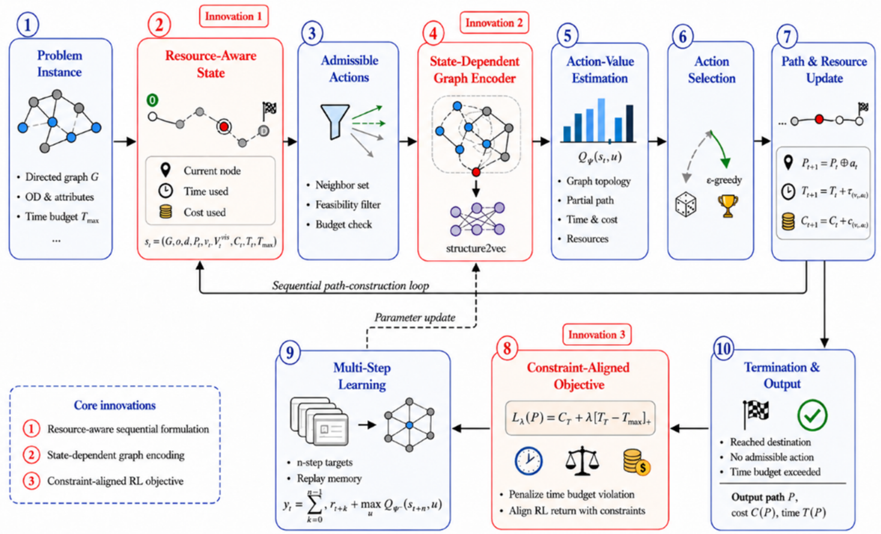Based on the defined MDP, the objective is to learn parameters Θ and ω so that $Q_{\mathsf{\Theta },\omega }\left(s_t,u\right)$ can accurately evaluate the long-term decision value of selecting candidate node u under the current partial path state s_t. After training, the learned value function is used to guide greedy path construction under feasibility masking. The complete pipeline of the proposed framework E2E_GERL is illustrated in Figure 1.

4.1. Training Procedure

For each training episode, a graph instance (G, o, d, T_max) is sampled from the training set. The agent starts from the origin node o and sequentially constructs the partial path. At each step t, the agent constructs the state s_t, computes structure2vec embeddings ${\mu }_v^{\left(t\right)}$, evaluates all feasible actions $u\in \mathcal{A}\left(s_t\right)$, and selects one candidate node according to an exploration policy.

The trainable model consists of two components. The first component is the structure2vec embedding module with parameters Θ, which maps graph structure, edge features, and path state features into node embeddings. The second component is the multi-layer neural network $f_{\omega }(·)$, which maps the state–action representation $h_{\mathsf{\Theta }}(s_t,u)$ to the action-value function $Q_{\mathsf{\Theta },\omega }\left(s_t,u\right)$. Defining Ψ = {Θ, ω} as the complete set of trainable parameters, the objective is to optimize Ψ so that $Q_{\mathsf{\Psi }}\left(s_t,u\right)$ accurately evaluates the long-term decision value of extending the path to candidate u.

4.2. Action-Value Function Learning via n-Step Q-Learning

The optimal action-value function satisfies the Bellman optimality equation:

$$Q^{\ast }\left(s_t,a_t\right)=r_t+\gamma \underset{u\in \mathcal{A}\left(s_{t+1}\right)}{\mathit{max}}{Q}^{\ast }\left(s_{t+1},u\right)$$

(24)

where γ is the discount factor. In E2E_GERL, the reward in Equation (12) is defined as the negative increment in the ReLU–Lagrangian path objective. We therefore use an undiscounted finite-horizon return with γ = 1. For a completed trajectory and a multiplier held fixed within the episode, ${\sum }_{t=0}^{K-1}{r}_t=L_{\lambda }\left(P_0\right)-L_{\lambda }\left(P_K\right)=-L_{\lambda }\left(P_K\right)$, where $L_{\lambda }\left(P_0\right)=0$. Hence, maximizing cumulative return is exactly equivalent to minimizing the terminal penalized path objective over completed trajectories. For γ < 1, later cost and constraint-violation increments would receive smaller weights, and this equality would no longer hold.

In the proposed framework, $Q^{\ast }\left(s_t,a_t\right)$ is approximated by $Q_{\mathsf{\Psi }}\left(s_t,a_t\right)$. The action-value function is trained to estimate the long-term consequence of extending the current partial path by one candidate node. This is important for the time-constrained SPP because a locally low-cost edge may lead to future infeasibility, while a locally more expensive edge may preserve resource feasibility and lead to a better final path.

Although γ = 1 preserves objective alignment, the consequences of an action may still emerge only after several subsequent path extensions. We therefore employ n-step Q-learning to improve credit assignment for such delayed effects. With γ = 1, the n-step return is as follows:

$$R_t^{\left(n\right)}={\sum }_{k=0}^{n-1}{r}_{t+k}$$

(25)

If the episode does not terminate within the next n steps, the target value is as follows:

$$y_t=R_t^{\left(n\right)}+{\gamma }^n\underset{u\in \mathcal{A}\left(s_{t+n}\right)}{\mathit{max}}{Q}_{\overline{\Psi }}\left(s_{t+n},u\right)$$

(26)

where $Q_{\overline{\mathsf{\Psi }}}$ is the target network used to stabilize training. If the episode terminates before or at step t + n, the target is simply $y_t=R_t^{\left(n\right)}$. The model parameters Ψ are updated by minimizing the Mean Squared Error (MSE) loss across a sampled mini-batch B. For a mini-batch B sampled from the replay memory, the training loss is as follows:

$$\mathcal{J}\left(\Psi \right)={\displaystyle \frac{1}{\left|\mathcal{B}\right|}}{\sum }_{(s_t,a_t,y_t)\in \mathcal{B}}{(Q_{\Psi }\left(s_t,a_t\right)-y_t)}^2$$

(27)

The model parameters Ψ are updated by minimizing Equation (27) using Adam optimizer. The target network parameters $\overline{\mathsf{\Psi }}$ are periodically synchronized with Ψ, or updated by a soft update rule:

$$\overline{\Psi }\leftarrow \tau \Psi +(1-\tau )\overline{\Psi }$$

(28)

where τ ∈ (0, 1] is the target update coefficient.

4.3. Balancing Exploration and Exploitation

During training, the agent follows an ϵ-greedy policy strictly bounded by the feasible action set $\mathcal{A}\left(s_t\right)$:

$$a_t=\left\{\begin{array}{cc}arandomnodefromA\left(s_t\right),\hfill & \hfill withprobabilityϵ\\ arg\underset{u\in \mathcal{A}\left(s_t\right)}{\mathit{max}}{Q}_{\Psi }\left(s_t,u\right),\hfill & \hfill withprobability1-ϵ\end{array}\right.$$

(29)

To effectively balance exploration and exploitation, ϵ is fixed or decayed gradually across episodes: ${ϵ}_l=\mathrm{m}\mathrm{a}\mathrm{x}({ϵ}_{min},{ϵ}_0·{\mathsf{\alpha }}_{\epsilon }^l)$, where l is the episode index, ϵ₀ is the initial exploration rate, ϵ_min is the minimum exploration rate and ${\mathsf{\alpha }}_{\epsilon }^l\in (0,1]$ is the decay factor. A larger ϵ encourages the agent to explore different path structures, while a smaller ϵ makes the agent rely more heavily on the learned value function.

4.4. Episode Termination and Fitted Q-Iteration

The feasible action mask is applied during the training procedure. This mask ensures that the selected action is valid and prevents the constructed path from revisiting nodes. In the training, an episode will terminate if (1) the destination node d is reached, (2) the feasible action set $\mathcal{A}\left(s_t\right)$ becomes empty before reaching d, or (3) the maximum path length $H_{max}$ is met. Reaching the destination and failing to reach the destination are treated differently. A completed path is evaluated using the ReLU–Lagrangian path objective in Equation (5), irrespective of whether its time budget is satisfied. In contrast, a trajectory terminated before reaching d is an incomplete path and receives an auxiliary terminal failure penalty −M. Let $c^{max}=\underset{(u,v)\in E}{\max }{c}_{uv}$ and $t^{max}=\underset{(u,v)\in E}{\max }{t}_{uv}$; a conservative upper bound on the penalized objective of any completed simple path is as follows:

$$U=H_{max}{c}^{max}+{\lambda [H_{max}{t}^{max}-T_{max}]}_{+}$$

(30)

We therefore define $M=\kappa U$, where $\kappa >1$. This construction makes the incomplete-path penalty scale with the graph instance and ensures that an incomplete trajectory is assigned a lower terminal value than any completed simple path under the bounded multiplier. The safety factor κ is selected on the validation set.

To improve sample efficiency and reduce the correlation among consecutive transitions, E2E–GERL uses an experience replay memory $\mathcal{M}$. During training, the generated transitions are stored in the $\mathcal{M}$ tuples as $(s_t,a_t,R_t^{\left(n\right)},s_{t+n},done)$, where done indicates whether the episode terminates at step t + n or before it.

At each update step, a mini-batch B is randomly sampled from $\mathcal{M}$. The target y_t is computed according to Equation (26), and the model parameters are updated by minimizing the loss in Equation (27). This process follows the fitted Q-iteration principle [67], where the function approximator is repeatedly fitted to Bellman target values generated from stored transitions.

After training, the learned action-value function is used for path construction. The framework executes the deterministic path construction policy $a_t^{\ast }=arg{max}_{u\in \mathcal{A}\left(s_t\right)}{Q}_{\mathsf{\Psi }}\left(s_t,u\right)$ to yield stable and reliable solutions. The final output is the constructed path P, total cost C(P), total travel time T(P), and feasibility status. If T(P) ≤ T_max, the path is feasible and its reported objective value is C(P). Otherwise, the path is evaluated by the penalized objective in Equation (5).

The entire training procedure of E2E_GERL with structure2vec is shown in Algorithm 1:

Algorithm 1: Training procedure of E2E_GERL with structure2vec

1: Initialize structure2vec parameters Θ and value-network parameters ω. Set Ψ ← {Θ, ω}. 2: Initialize target network parameters $\overline{\mathsf{\Psi }}\leftarrow \mathsf{\Psi }$. 3: Initialize experience replay memory $\mathcal{M}$ with capacity N. 4: for episode l = 1, 2, …, L do 5:     Sample a training instance $\left(G,o,d,T_{max}\right)$ from training graph dataset ${\mathcal{D}}_{train}$. 6:     Initialize partial path $P_0=\left(o\right)$, visited set $V_0^{vis}=\left\{o\right\}$, cumulative cost $C_0=0$, and time $T_0=0$. 7:     Update exploration probability ${ϵ}_l\leftarrow \mathrm{m}\mathrm{a}\mathrm{x}({ϵ}_{min},{ϵ}_0·{\mathsf{\alpha }}_{\epsilon }^l)$. 8:     for step t = 0, 1, …, $H_{max}$ do 9:        Construct current state $s_t=(G,v_t,d,V_t^{vis},C_t,T_t,T_{max})$. 10:       Construct feasibility mask $\mathcal{A}\left(s_t\right)=\left\{u\in V|\left(v_t,u\right)\in E,u\notin V_t^{vis}\right\}$. 11:       if $\mathcal{A}\left(s_t\right)=\mathsf{\varnothing }$ and $v_t\ne d$ then 12:         Assign terminal penalty −M and terminate the episode. 13:         break 14:       end if 15:       Compute structure2vec node embeddings ${\left\{{\mu }_v^{\left(t\right)}\right\}}_{v\in V}$ using parameters Θ. 16:       Select action $a_t$ using the ϵ-greedy policy over the masked set $\mathcal{A}\left(s_t\right)$: $${\mathrm{a}}_t=\left\{\begin{array}{cc}\mathrm{a}\mathrm{random}\mathrm{node}\mathrm{from}A\left(s_t\right),\hfill & \hfill \mathrm{with}\mathrm{probability}\mathsf{ϵ}\\ arg\underset{u\in \mathcal{A}\left(s_t\right)}{\mathit{max}}{Q}_{\mathsf{\Psi }}\left(s_t,u\right),\hfill & \hfill \mathrm{with}\mathrm{probability}1-\mathsf{ϵ}\end{array}\right.$$ 17:       Execute ${\mathrm{a}}_t$: append ${\mathrm{a}}_t$ to $P_t$, update $V_{t+1}^{vis}\leftarrow V_t^{vis}\bigcup \left\{{\mathrm{a}}_t\right\}$. 18:       Update accumulators: $C_{t+1}\leftarrow C_t+c_{v_t{a}_t}$ and $T_{t+1}\leftarrow T_t+t_{v_t{a}_t}$. 19:       Update state $s_{t+1}=(G,a_t,d,V_{t+1}^{vis},C_{t+1},T_{t+1},T_{max})$. 20:       Calculate state-level penalized cost $\mathsf{\Phi }\left(s_{t+1}\right)\leftarrow C_{t+1}+{\mathsf{\lambda }[T_{t+1}-{\mathrm{T}}_{\mathrm{m}\mathrm{a}\mathrm{x}}]}_{+}$. 21:       Compute reward $r_t\leftarrow -(\mathsf{\Phi }\left(s_{t+1}\right)-\mathsf{\Phi }(s_t\left)\right)$. 22:       Store transition information for n-step return construction. 23:       if an n-step transition is available then 24:         Compute $R_t^{\left(n\right)}={\sum }_{k=0}^{n-1}{r}_{t+k}$. 25:         Insert tuple $(s_t,a_t,R_t^{\left(n\right)},s_{t+n},\mathrm{d}\mathrm{o}\mathrm{n}\mathrm{e})$ into replay memory $\mathcal{M}$. 26:       end if 27:       if $\left|\mathcal{M}\right|\ge \mathcal{B}$ then 28:       Sample a random mini-batch $\mathcal{B}$ from $\mathcal{M}$. 29:       for each tuple i in $\mathcal{B}$ do 30:          if episode is terminated before or at $t+n$ then $y_i=R_i^{\left(n\right)}$ 31:          else $y_i=R_i^{\left(n\right)}+{\gamma }^n\underset{u\in \mathcal{A}\left(s_{i+n}\right)}{\mathit{max}}{Q}_{\overline{\mathsf{\Psi }}}\left(s_{i+n},u\right)$ 32:        end for 33:        Update Ψ by minimizing MSE loss: $\mathcal{J}\left(\mathsf{\Psi }\right)={\displaystyle \frac{1}{\mathcal{B}}}\sum _{i\in \mathcal{B}}{(Q_{\mathsf{\Psi }}\left(s_i,a_i\right)-y_i)}^2$ 34:        Softly update target network: $\overline{\mathsf{\Psi }}\leftarrow \tau \mathsf{\Psi }+(1-\tau )\overline{\mathsf{\Psi }}$. 35:        end if 36:        if $a_t=d$ then 37:          Terminate the episode. 38:            break 39:        end if 40:     end for 41: end for 42: return $\mathsf{\Psi }$

5. Numerical Experiments

This section evaluates the effectiveness, efficiency and generalization ability of the proposed E2E–GERL framework for the time-constrained SPP.

5.1. Datasets and Instance Generation

Existing standard benchmark datasets, such as the Solomon benchmark [68], are ill-suited for the specific SPP constraints addressed in this study and thus could not be directly utilized. To bridge this gap, we construct a custom dataset employing two complementary strategies.

The first phase entails generating a subset of data via simulation. After reviewing the relevant literature, we decide to generate graph instances using the Erdős-Rényi (ER) models [69], as this type of graph is commonly used to simulate many real-world networks. We first specify a range for the number of nodes and then randomly sample the number of nodes from this range using a uniform distribution. Then, we use this number to generate a graph based on the ER model. For our experiment, we vary the training and test graph sizes in the ranges {7–15, 20–30, 40–60, 70–100, 100–150}.

Nevertheless, relying solely on simulated data may lack sufficient empirical robustness. To address this, we implement a second strategy: adapting established benchmarks to our specific context. Guided by the SPP’s inherent characteristics, we perform targeted modifications on an extended version of the standard Solomon benchmark, which is the Gehring and Homberger benchmark [70] whose sizes are {200, 400, 600, 800}. This process involves calibrating specific parameters to meet our structural requirements while strictly preserving essential original data elements. Consequently, the performance of the proposed method E2E_GERL is rigorously evaluated using both the synthetic and the modified benchmark datasets.

5.2. Constraint Generation

For each graph instance, the time constraint is generated relative to the unconstrained shortest path. A valid time-constrained shortest path instance should satisfy two requirements. The first requirement is that the prescribed time constraint must allow for at least one feasible path from the origin to the destination. The second requirement is that the time constraint must be sufficiently restrictive to exclude the unconstrained minimum cost path. Otherwise, the constrained problem has the same optimal solution as the ordinary shortest path problem and the effect of the proposed constraint-handling mechanism cannot be meaningfully evaluated. For each graph and origin–destination pair, two reference paths are therefore computed before assigning the time constraint.

First, the unconstrained minimum cost path is obtained as follows:

$$P_i^c=arg\underset{P\in P_i}{\min }C\left(P\right)$$

(31)

where $P_{\mathrm{i}}$ denotes the set of all valid paths from the origin to the destination at instance $i$ and $C\left(P\right)={\sum }_{(u,v)\in P}{c}_{uv}$. Its total travel time is denoted by the following:

$$T_i^c=T(P_i^c)={\sum }_{(u,v)\in P_i^c}{t}_{uv}$$

(32)

When multiple paths have the same minimum cost, a rule is adopted: cost is minimized first, and travel time is minimized second. This ensures that $T_i^c$ is the smallest travel time among all unconstrained minimum cost paths. Consequently, any constraint satisfying $T_{max,i}<T_i^c$ excludes every unconstrained minimum cost solution rather than only one arbitrarily selected path.

Second, the minimum time path is computed as follows:

$$P_i^t=arg\underset{P\in P_i}{\min }T\left(P\right)$$

(33)

Its total travel time is $T_i^t=T\left(P_i^t\right).$ When multiple paths have the same minimum travel time, cost is used as the secondary criterion. Because $P_i^t$ is the fastest path between the specified nodes, any constraint satisfying $T_{max,i}\ge T_i^t$ guarantees that the feasible set is nonempty. The time constraint is then generated within the interval between the minimum time path and the unconstrained minimum cost path:

$$T_{max,i}=T_i^t+\delta \left(T_i^c-T_i^t\right),0<\delta <1$$

(34)

where $\delta$ controls the tightness of the time constraint. This construction guarantees $T_i^t\le T_{max,i}<T_i^c$. Therefore, the minimum time path remains feasible, whereas the unconstrained minimum cost path is infeasible. The constrained optimization problem must consequently identify a path that explicitly balances transportation cost and travel time.

5.3. Evaluation Metrics

The performance of the compared methods is evaluated based on solution feasibility and solution quality. Because a path with a low transportation cost may violate the prescribed time constraint, objective values are interpreted only together with feasibility information. CPLEX is used as the sole reference solver throughout the experiments.

Let $P_i^m$ denote the path returned by method $m$ for test instance $i$, where $i\in 1,\dots ,N$. Its total transportation cost and total travel time are denoted by $C_i^m=C\left(P_i^m\right)$ and $T_i^m=T\left(P_i^m\right)$. A returned solution is considered feasible only if it satisfies all structural and resource requirements of the problem. Specifically, the path must satisfy $T_i^m\le T_{max,i}$. The feasibility indicator is defined as follows:

$$I_i^m=\left\{\begin{array}{cc}1,& if{P}_i^{m}isavalidtime-feasiblepath\\ & 0,otherwise\end{array}\right.$$

(35)

The feasibility rate (fsb%) of method $m$ over $N$ test instances is calculated as follows:

$${\displaystyle \frac{1}{N}}{\sum }_{i=1}^N{I}_i^m\times 100\%$$

(36)

The feasibility rate is reported for every exact, approximate and NCO method. An infeasible path is not treated as a valid solution, even if its transportation cost is lower than that of the feasible solutions returned by the other methods. If a method does not produce any feasible solution within a test group, its feasible objective value and relative solution quality metric are reported as not available. The feasible objective value is always presented together with the feasibility rate, thereby preventing a method with a low feasibility rate from appearing favorable merely because of a small number of low-cost feasible solutions.

For small-scale instances, CPLEX is allowed to run until global optimality is certified. Let $C_i^{{CPLEX}^{\ast }}$ denote the optimal objective value proved by CPLEX for instance $i$. For a feasible solution returned by method $m$, the optimality gap is defined as follows:

$${Gap}_{i,m}^{opt}={\displaystyle \frac{C_i^m-C_i^{{CPLEX}^{\ast }}}{C_i^{{CPLEX}^{\ast }}}}\times 100\%$$

(37)

This metric is used only when CPLEX has formally certified the global optimum. A value of zero indicates that the evaluated method obtains a solution with the same objective value as the certified CPLEX optimum, whereas a positive value indicates the relative cost increase with respect to that optimum. For medium and large-scale instances, CPLEX is executed under a predefined time limit 3600 s. If global optimality is not certified within this limit, the best feasible solution found by CPLEX is treated as a reference incumbent rather than as an exact optimum. Let $C_i^{{CPLEX}^{inc}}$ denote the objective value of the best feasible incumbent returned by CPLEX for instance $i$. The relative percentage deviation (RPD) gap of method $m$ from the CPLEX incumbent is defined as follows:

$${RPD}_{i,m}^{CPLEX}={\displaystyle \frac{C_i^m-C_i^{{CPLEX}^{inc}}}{C_i^{{CPLEX}^{inc}}}}\times 100\%$$

(38)

This quantity is referred to as the relative deviation from the CPLEX incumbent rather than the approximation ratio. When CPLEX has not proved global optimality, its incumbent cannot be interpreted as the exact optimal solution. Therefore, a negative value indicates that method $m$ finds a feasible solution with a lower cost than the best feasible solution obtained by CPLEX within 3600 s. It does not imply that the method outperforms the unknown global optimum. CPLEX itself has ${RPD}^{CPLEX}=0$ by definition. The CPLEX solver-reported incumbent-to-bound gap is reported separately and is not used as the solution quality metric of the approximate and NCO methods.

All CPLEX experiments use IBM ILOG CPLEX 20.1.0 through the python interface on CPU. The number of solver threads is fixed at 1 for every instance, and the random seed is fixed at 5. For medium- and large-scale instances, the wall-clock time limit is 3600 s per query. Parallel mode is set to Auto. Presolve, cut generation, and MIP primal heuristics are left at the solver’s documented automatic defaults, and no problem-specific parameter tuning is performed on the test set.

5.4. Hyperparameter Tuning and Generalization Analysis

For our proposed method E2E_GERL, we adopt a pre-training approach, which involves initial training on small-scale graphs, then using the preliminary results to select suitable hyperparameters for the model, and finally applying it to large-scale graphs. In the case of the SPP, since the model will be trained on a large graph with 150 nodes, we use the model trained on small graphs as initialization for training on large graphs. This process is known as pre-training. After pre-training, a series of experiments are conducted to analyze the generalization of E2E_GERL.

5.4.1. Hyperparameter Tuning

The hyperparameters of E2E_GERL are shown in

Table 1. Hyperparameters of E2E_GERL.

Hyperparameter	Setting
Iteration rounds Kμ	4
Embedding dimension $d_{\mu }$	64
Batch size	64
n-step horizon	2
Discount factor γ	1
Exploration probability ${ϵ}_0$	0.1
Training episodes L	20,000
Maximum path length $H_{max}$	$\left|V\right|-1$
Terminal failure penalty M	$\mathsf{\kappa }\mathrm{U}$
Safety factor $\kappa$	1.1
Random seeds	10

.

For each graph instance, the time constraint is generated within the interval between the minimum time path and the unconstrained minimum cost path through tightness δ. A smaller δ produces a tighter time constraint because the budget is closer to the travel time of the minimum time path. Conversely, a larger δ provides greater flexibility but still excludes the unconstrained minimum cost path. 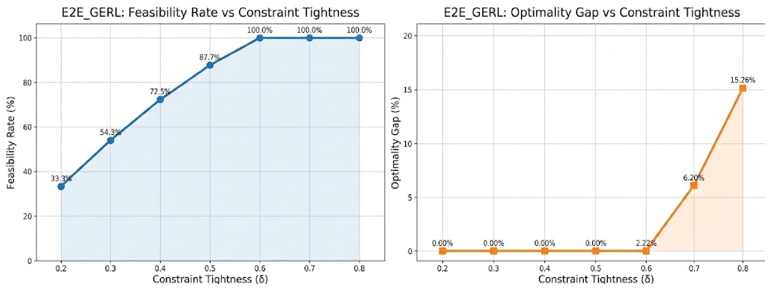To evaluate the impact of tightness δ on experimental solution feasibility and solution quality, we conduct tests using 30-node benchmark graphs. In the tests, seven constraint levels are considered: $\delta \in \{0.2,0.3,0.4,0.5,0.6,0.7,0.8\}$. As illustrated in Figure 2, these figures represent the impact of tightness δ on experimental solution feasibility and solution quality, and tests produce the most favorable results when δ is 0.6. Therefore, this setting is used in the subsequent experiments.

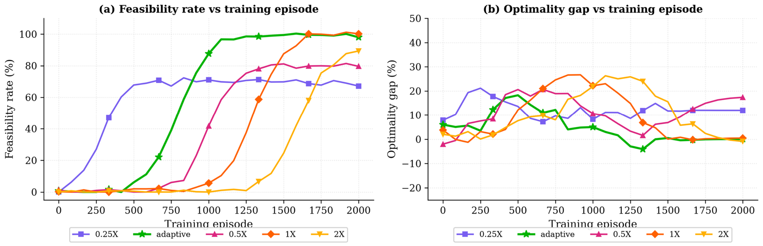
For the Lagrangian coefficient $\lambda$ in Equation (5), we initially apply an iterative primal–dual method with projected gradient updates to determine its value [71]. To quantify the role of the λ, we conduct controlled ablation on the 30-node benchmark graphs. A relatively large constant value X is set as $c^{max}$, where $c^{max}=\underset{(u,v)\in E}{\max }{c}_{uv}$ in the benchmark graphs. As a controlled comparison, we construct a fixed-λ variant as a constant during both training and inference in which the multiplier is set by the large constant X. We additionally evaluate $\lambda \in \{0.25X,0.5X,X,2X\}$. 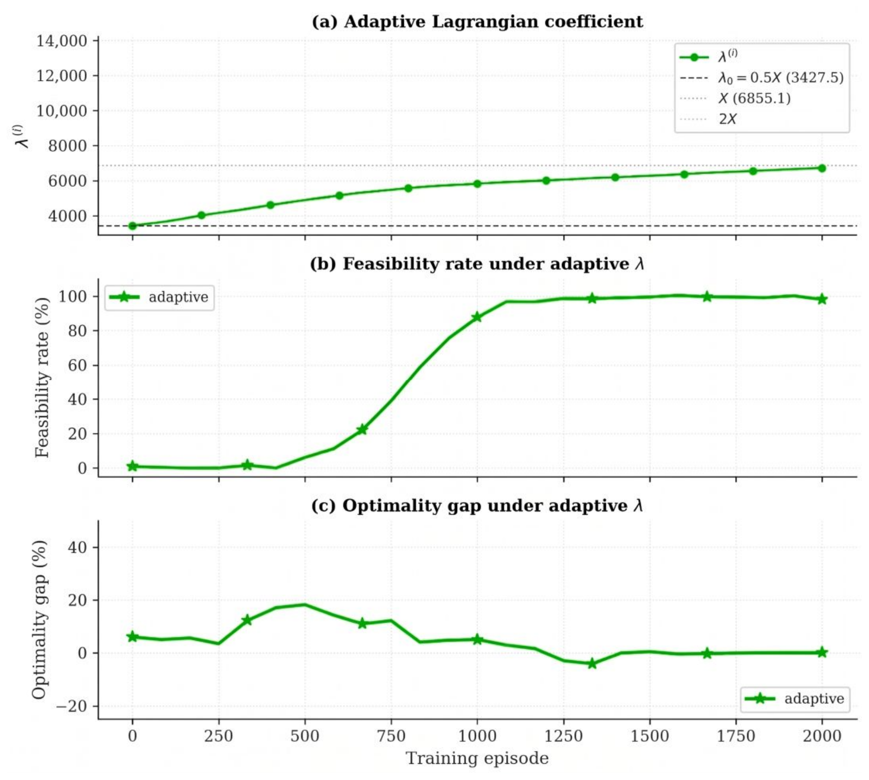As for the adaptive-λ variant, the initial ${\lambda }_0$ is set as 0.5X and it updates after every episode by the projected subgradient rule of Equation (6) with ${\eta }_{\lambda }=0$.1. As illustrated in Figure 3 and Figure 4, these figures represent the difference between the fixed coefficients and the adaptive coefficient on solution quality and feasibility. The results indicate that even though the large constant can obtain good solution quality and feasibility, it fluctuates more and requires many more training episodes than the adaptive λ. The adaptive λ achieves the most favorable results. The λ sensitivity analysis in Figure 3 and Figure 4 is restricted to the N = 30 validation graphs and is not independently repeated at the largest scales. Consequently, the large-scale experiments evaluate E2E_GERL under the stated size-scaled λ rule rather than establishing that the precise λ sensitivity profile observed at N = 30 is invariant to graph size.

To ensure reproducibility, we report the complete architecture and optimization settings of E2E_GERL. In addition to the multi-layer neural network $f_{\mathsf{\omega }}(·)$ and the edge transformation network ${\mathrm{\varnothing }}_{\mathrm{e}}(·)$, we use Adam optimizer to optimize all model parameters Ψ with a learning rate $\eta =1\times {10}^{-4}$. The learning rate schedule of Adam is constant, weight decay is 0, ${\beta }_1$ is 0.9 and ${\beta }_2$ is 0.999. Gradients are clipped at 1.0 and mini-batches of 64 transitions are sampled from a replay buffer of capacity 5000. For other training parameters, the discount factor is fixed at γ = 1 and is not tuned. The initial exploration probability is set to ϵ = 0.1. The maximum number of training episodes L is 20,000. The maximum iteration episodes L was is to 20,000. For n-step Q-learning, n is set to 2.

5.4.2. Generalization Analysis

In the experiments mentioned above, we train our method E2E_GERL on instances of the same size for experiments of different scales. A central motivation for using a structure2vec-based policy is that the learned graph representation and value function can be transferred across graph sizes. To evaluate this property, we train E2E_GERL on graphs of both the synthetic and modified benchmark dataset with varying numbers of nodes and then test its performance on graphs of larger sizes to demonstrate its generalization ability. The results are shown in

Table 2. E2E_GERL’s performance on the synthetic dataset.

	Test	10	20	30	50	100	150
Train
8		0.00%	0.00%	0.52%	2.35%	3.37%	5.88%
15			0.00%	0.03%	0.86%	1.43%	4.15%
30				0.01%	0.72%	1.00%	2.72%
50					0.03%	0.71%	1.62%
80						0.18%	0.66%

and

Table 3. E2E_GERL’s performance on the synthetic and modified Gehring and Homberger benchmark dataset.

	Test	200	400	600	800
Train
50		7.79%	9.08%	11.54%	14.29%
100		2.63%	3.21%	4.82%	6.34%
200		0.47%	0.93%	1.50%	2.92%

.

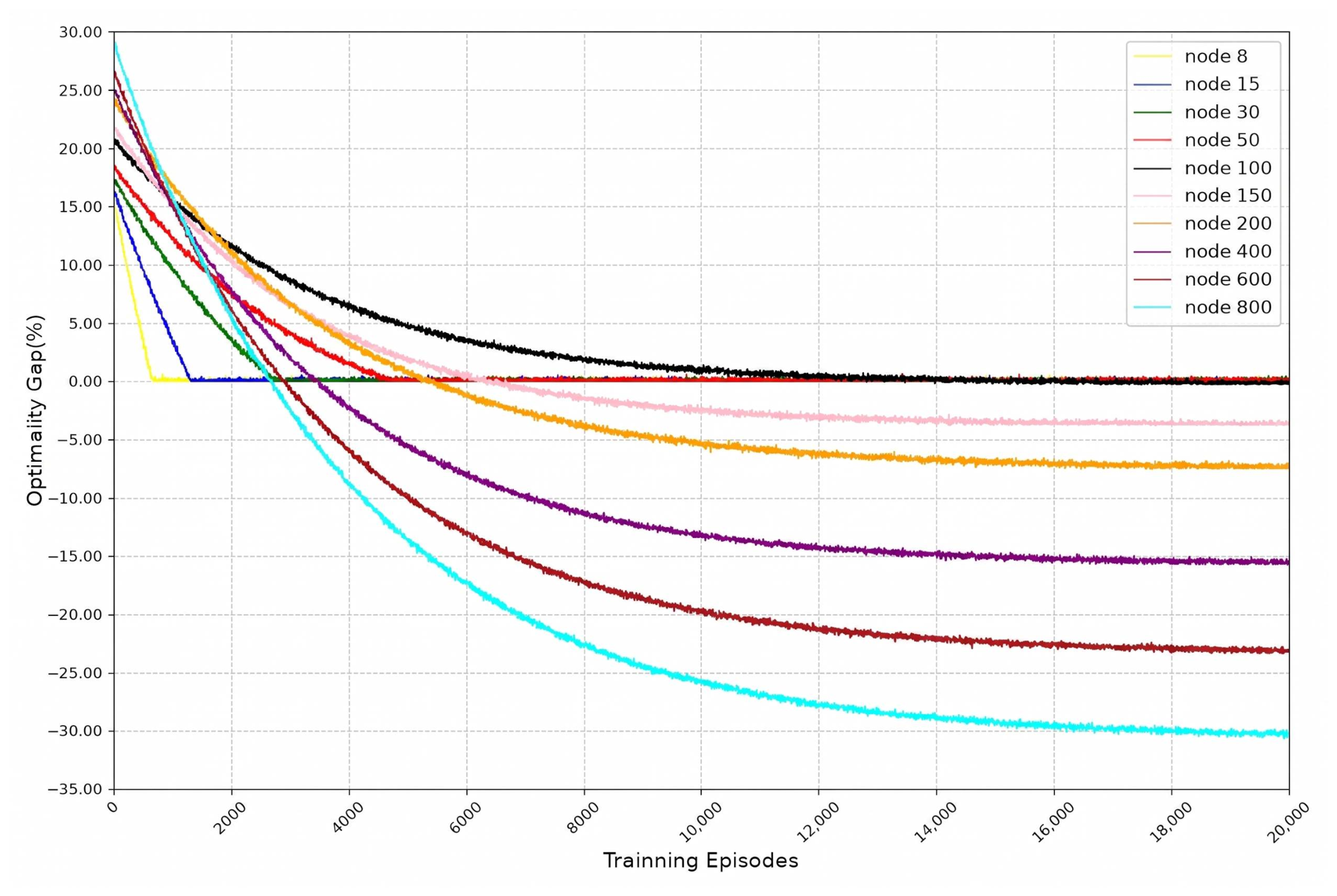
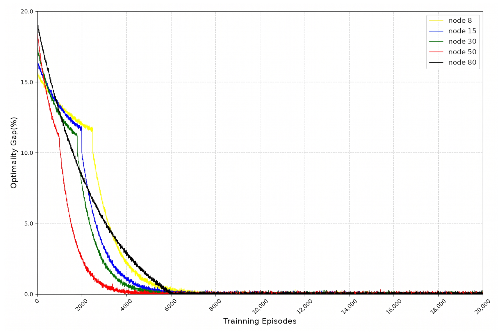
To better demonstrate the generalization ability of our method E2E_GERL, we apply models trained on graphs of the synthetic dataset with 8, 15, 30, 50, and 80 nodes, respectively, to solve problems on a larger-scale graph with 150 nodes. The results are shown in Figure 5.

These results support the claim that structure2vec-based policy provides meaningful generalization ability. However, the performance degradation observed when training on very small graphs and testing on much larger graphs indicates that pre-training should be complemented by fine-tuning or curriculum learning when the target graph size is substantially larger than the training size.

5.5. Convergence of E2E_GERL

In Figure 6, we demonstrate the convergence of our algorithm E2E_GERL through the experimental results presented. During experiments conducted at different scales, we plot the convergence curves of the algorithm during the learning and training process.

Figure 5 and Figure 6 show that our algorithm converges nicely. We employ a pre-training approach to train the model on small-scale graphs and subsequently extend it to large-scale instances. The algorithm also exhibits rapid convergence, thus making our algorithm highly suitable for problems of varying sizes.

5.6. Baselines and Constraint Adaptions

As mentioned earlier, existing research on solving the SPP often involves using exact, approximate and NCO algorithms. We have selected and adapted some classic and state-of-the-art baselines from these methods for comparison purposes. All baselines receive the same graph instance G, origin o, destination d, and time budget $T_{max}$. Solutions returned by every method are independently re-evaluated using the same feasibility checker, which verifies source–destination connectivity, directed-edge validity, non-repetition, and the cumulative time constraint.

We use CPLEX as the sole reference solver throughout the experiments, and it solves the mathematical model in Equations (1)–(4) directly.

Labeling algorithms constitute the predominant class of methods for solving the constrained SPP, with the Bidirectional Dijkstra (BD) algorithm serving as a widely established benchmark. The classical BD algorithm solves the unconstrained shortest path problem and therefore cannot be applied directly to this problem. In the experiments, we use a resource-constrained bidirectional label-setting algorithm (RC-BD) [19]. Each forward and backward label records both accumulated routing cost and travel time. Labels exceeding the time budget or failing a remaining-time lower-bound test are pruned, and Pareto dominance is applied at each node. Forward and backward labels can be joined only when their combined travel time does not exceed $T_{\mathrm{m}ax}$.

In terms of approximate algorithms, we select the classical heuristic algorithm Ant Colony Optimization (ACO) for comparison. The SPP is one of the several successful applications of ACO [72], and ACO algorithms can be useful for quickly finding high-quality solutions in the SPP. During the construction of paths by the ant colony, at every node expansion step each ant checks to find out whether the accumulated travel time exceeds $T_{max}$. Once this threshold is exceeded, the ant is immediately terminated, contributing no pheromone to the global optimal path pool and thus prohibited from completing its search. This enforces the constraint ensuring that all generated paths satisfy the time constraint through early pruning.

We also compare an augmented algorithm, Learning to Improve (L2I), which combines machine learning methods but does not have an end-to-end structure [73]. We adapt L2I to the time-constrained SPP by establishing an intra-route action space including 2-Opt, symmetric exchanges and relocations so that the controller learns the distinct dynamics of each move size. We also replace the encoder with a 4-dim feature embedded through an 8-head self-attention layer, mean-pooled across nodes and concatenated with the running H-step history, then fed to a two-layer MLP. The time constraint $T_{max}$ is enforced by hard rejection: every operator candidate is checked end-to-end against $T_{max}$ and discarded if infeasible.

To address the limitation that classical baselines alone are insufficient for evaluating a graph-embedded reinforcement learning method, we also compare some state-of-the-art NCO baselines. The Attention Model (AM) is adopted as a neural routing baseline [47] and the Graph Attention Network (GAT) is adopted as a graph neural network baseline [61]. Neither the AM nor the GAT are treated as unconstrained off-the-shelf solvers, and they are re-trained on the same training instances and time budget distributions as E2E_GERL and are adapted to the sparse origin-to-destination setting. Their decoders use the stated adjacency and visited-node restrictions and receive the resource information required by the constrained problem. For the GAT comparison, we additionally use a controlled encoder replacement configuration in which the state representation, Q-learning procedure, reward, decoder, training data, and computational budget are held fixed and only the structure2vec encoder is replaced by the GAT. This makes the representation comparison directly interpretable. Due to computational resource limitations, we conduct training on graphs with a maximum of 150 nodes.

5.7. Performance Comparison

Next, we compare our proposed E2E_GERL method with the baselines through comparative experiments. Each cell aggregates K = 100 independently generated fixed test instances. E2E_GERL, the AM, and the GAT are independently trained using R = 10 random seeds; values are reported as the mean ± standard deviation across the 10 complete training runs. CPLEX and RC-BD are executed once per instance, and ACO is evaluated under independent random seeds using the same declared computational budget.

In

Table 4. Average objective, computing times, optimality gap and feasibility rate with standard deviations of each method on synthetic dataset (N = 8, 15).

	N = 8				N = 15
Method	Obj.	Time (s)	Gap%	Fsb%	Obj.	Time (s)	Gap%	Fsb%
CPLEX	335	0.23	0.00%	100%	443	1.22	0.00%	100%
RC-BD	335	0.05	0.00%	100%	443	0.53	0.00%	100%
ACO	335	0.04	0.00 ± 0.00%	100 ± 0.00%	443	0.05	0.00 ± 0.00%	100 ± 0.00%
L2I	335	0.03	0.00 ± 0.00%	100 ± 0.00%	443	0.05	0.00 ± 0.00%	100 ± 0.00%
AM	335	0.05	0.00 ± 0.00%	100 ± 0.00%	443	0.05	0.00 ± 0.00%	100 ± 0.00%
GAT	335	0.05	0.00 ± 0.00%	100 ± 0.00%	443	0.06	0.00 ± 0.00%	100 ± 0.00%
E2E_GERL	335	0.05	0.00 ± 0.00%	100 ± 0.00%	443	0.06	0.00 ± 0.00%	100 ± 0.00%

,

Table 5. Average objective, computing times, optimality gap and feasibility rate with standard deviations of each method on synthetic dataset (N = 30, 50).

	N = 30				N = 50
Method	Obj.	Time (s)	Gap%	Fsb%	Obj.	Time (s)	Gap%	Fsb%
CPLEX	678	51.60	0.00%	100%	1537	261.47	0.00%	100%
RC-BD	678	3.63	0.00%	100%	1537	10.47	0.00%	100%
ACO	681.15	0.57	0.46 ± 0.03%	100 ± 0.00%	1586.35	1.63	3.21 ± 0.34%	100 ± 0.00%
L2I	695.33	0.53	2.53 ± 0.32%	97.25 ± 0.04%	1594.28	1.72	3.67 ± 0.57%	95.69 ± 0.12%
AM	681.92	0.14	0.57 ± 0.02%	99.41 ± 0.01%	1606.64	1.14	4.45 ± 0.07%	98.57 ± 0.01%
GAT	678.51	0.12	0.06 ± 0.01%	99.83 ± 0.01%	1576.40	0.38	2.58 ± 0.04%	99.23 ± 0.01%
E2E_GERL	678	0.15	0.00 ± 0.00%	100 ± 0.00%	1537	0.23	0.00 ± 0.00%	100 ± 0.00%

,

Table 6. Average objective, computing times, RPD to CPLEX incumbent and feasibility rate with standard deviations of each method on synthetic dataset (N = 100, 150).

	N = 100				N = 150
Method	Obj.	Time (s)	RPD%	Fsb%	Obj.	Time (s)	RPD%	Fsb%
CPLEX	4593.18	3600	0.00%	100%	10,985.26	3600	0.00%	100%
RC-BD	4582	38.52	−0.24%	100%	10,544.25	646.51	−4.01%	100%
ACO	4855.42	7.35	5.73 ± 0.58%	100 ± 0.00%	11,648.18	17.15	6.03 ± 0.83%	100 ± 0.00%
L2I	4888.20	2.83	6.45 ± 0.82%	92.74 ± 0.61%	11,741.94	4.28	6.81 ± 1.02%	90.63 ± 0.81%
AM	4972.59	2.57	8.35 ± 0.15%	95.66 ± 0.07%	11,408.37	5.62	3.75 ± 0.24%	94.51 ± 0.11%
GAT	4814.73	0.41	4.78 ± 0.07%	98.91 ± 0.04%	11,268.38	0.54	2.56 ± 0.14%	96.85 ± 0.07%
E2E_GERL	4582	0.32	−0.24 ± 0.00%	100 ± 0.00%	10,578.93	0.46	−3.70 ± 0.02%	100 ± 0.00%

,

Table 7. Average objective, computing times, RPD to CPLEX incumbent and feasibility rate with standard deviations of each method on modified Gehring and Homberger benchmark dataset (N = 200, 400).

	N = 200				N = 400
Method	Obj.	Time (s)	RPD%	Fsb%	Obj.	Time (s)	RPD%	Fsb%
CPLEX	3821.56	3600	0.00%	100%	7752.64	3600	0.00%	100%
RC-BD	3585.83	3600	−6.17%	100%	6835.50	3600	−11.83%	100%
ACO	3854.80	38.66	0.81 ± 0.67%	100 ± 0.00%	7653.25	82.58	−1.22 ± 0.94%	100 ± 0.00%
L2I	3913.25	4.47	2.31 ± 1.52%	86.12 ± 1.92%	7925.18	6.35	2.24 ± 1.77%	81.73 ± 2.63%
AM	3845.71	7.25	0.55 ± 0.27%	91.94 ± 0.19%	7754.45	8.82	0.06 ± 0.31%	90.42 ± 0.26%
GAT	3832.42	0.71	0.21 ± 0.17%	95.78 ± 0.11%	7143.56	0.88	−7.76 ± 0.25%	94.24 ± 0.14%
E2E_GERL	3535.74	0.54	−7.48 ± 0.03%	100 ± 0.00%	6533.11	0.57	−15.73 ± 0.05%	99.95 ± 0.02%

and

Table 8. Average objective, computing times, RPD to CPLEX incumbent and feasibility rate with standard deviations of each method on modified Gehring and Homberger benchmark dataset (N = 600, 800).

	N = 600				N = 800
Method	Obj.	Time (s)	RPD%	Fsb%	Obj.	Time (s)	RPD%	Fsb%
CPLEX	18,732.96	3600	0.00%	100%	33,725.63	3600	0.00%	100%
RC-BD	15,040.69	3600	−19.71%	100%	25,091.86	3600	−25.60%	100%
ACO	17,952.53	367.58	−4.21 ± 1.65%	100 ± 0.00%	30,532.15	1958.33	−9.60 ± 2.18%	100 ± 0.00%
L2I	19,067.85	10.25	1.75 ± 2.39%	74.26 ± 4.14%	33,847.29	11.80	0.36 ± 3.52%	65.31 ± 6.42%
AM	17,446.22	16.57	−6.73 ± 0.52%	86.25 ± 0.34%	31,493.58	35.28	−7.14 ± 0.79%	80.82 ± 0.53%
GAT	15,718.04	0.91	−16.27 ± 0.31%	92.66 ± 0.26%	24,985.91	1.15	−25.97 ± 0.43%	88.46 ± 0.30%
E2E_GERL	14,355.16	0.67	−23.34 ± 0.09%	96.19 ± 0.06%	23,363.83	0.92	−30.81 ± 0.14%	94.34 ± 0.12%

, we compare the performance of our algorithm with the previously mentioned CPLEX, RC-BD, ACO, L2I, AM and GAT on the synthetic and modified Gehring and Homberger benchmark dataset.

As illustrated in Table 4, Table 5 and Table 6, E2E_GERL demonstrates superior performance on the synthetic dataset, yielding higher solution accuracy and shorter computing times compared to the baseline algorithms. Notably, this performance advantage scales effectively with graph size. Furthermore, the results presented in Table 7 and Table 8 confirm that our algorithm consistently outperforms competing algorithms on the large-scale modified Gehring and Homberger benchmark dataset. Notably, some algorithms can sometimes achieve better results with a lower cost than the best feasible solution obtained by CPLEX within 3600 s, but it does not imply that the algorithms outperform the unknown global optimum.

The experiments show that the solution quality of E2E_GERL is very good, indicating its excellent generalization ability.

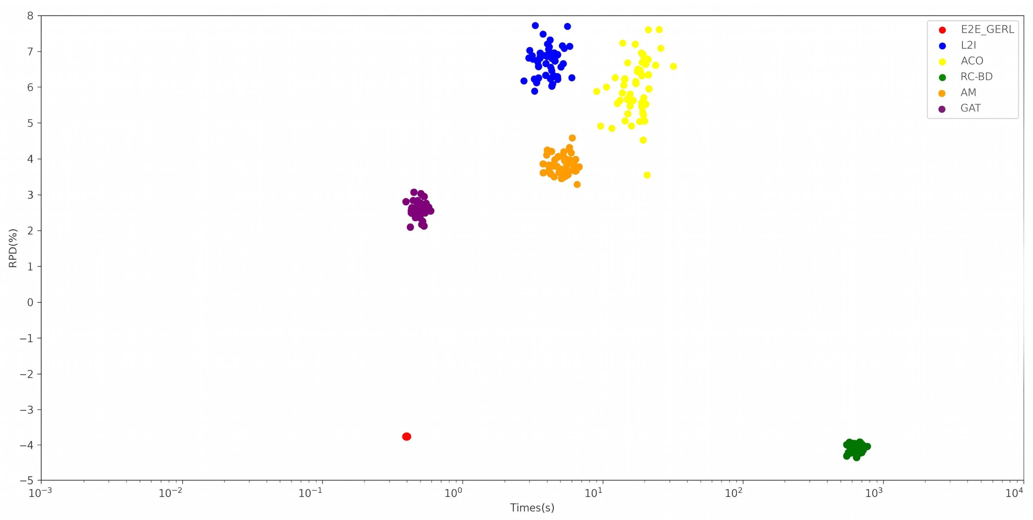
Figure 7 illustrates the time taken by each method to terminate the run and the solution quality they ultimately achieved. In the figure, our algorithm is obviously quicker than other methods while achieving even better solution quality.

5.8. Ablation Study

To strictly evaluate the independent contribution of each component, we conduct a comprehensive ablation study by removing or replacing one component at a time while keeping the other settings unchanged on the N = 50 and N = 150 synthetic datasets by training with 10 random seeds. Three main variants are recommended.

The first is without structure2vec. This variant removes the structure2vec-based graph embedding module. The action-value function is learned using only local edge features and resource-related state features, such as edge cost, edge time, accumulated cost, accumulated travel time, and remaining time limit.

The second is without the ReLU–Lagrangian penalty. This variant removes the penalty term ${\lambda [T\left(P\right)-T_{max}]}_{+}$ from the learning objective. The reward is defined only according to the cost.

The third is one-step Q-learning. This variant replaces the n-step Q-learning with standard one-step temporalmdifference learning.

The ablation results are shown in

Table 9. Ablation study of E2E_GERL.

	N = 50				N = 150
Variant	Obj.	Time (s)	Gap%	Fsb%	Obj.	Time (s)	RPD%	Fsb%
Full E2E_GERL	1537	0.23	0.00 ± 0.00%	100 ± 0.00%	10,578.93	0.46	−3.70 ± 0.02%	100 ± 0.00%
w/o structure2vec	1652.56	2.62	7.52 ± 1.68%	96.53 ± 0.24%	12,188.37	6.27	10.92 ± 3.58%	91.74 ± 0.36%
w/o ReLU-Lagrangian penalty	1537	0.06	0.00 ± 0.00%	64.68 ± 12.64%	10,546.52	0.12	−3.97 ± 0.02%	46.14 ± 24.20%
1-step Q-learning	1537	0.75	0.00 ± 0.00%	99.62 ± 0.02%	10,623.71	1.02	−3.36 ± 0.03%	98.37 ± 0.15%

.

The comparison between the full E2E_GERL and that without structure2vec evaluates the role of graph-structured representation learning. Without the structure2vec module, the model relies mainly on local edge and resource features and cannot sufficiently capture the structural context of candidate nodes. As a result, it makes more myopic path extension decisions, especially on large-scale graphs. Degradation in optimality gap, RPD to CPLEX incumbent and feasibility rate indicates that the structure2vec is important for identifying candidate nodes under the current partial path state.

The result of that without the ReLU–Lagrangian penalty reveals the effect of explicit constraint embedding. When the penalty term is removed, the agent receives no direct feedback of time constraint violation and tends to optimize traversal cost alone. Therefore, this variant may generate paths with low cost but poor feasibility. A significantly lower feasibility rate demonstrates that the ReLU–Lagrangian penalty is essential for guiding the policy into the feasible solutions.

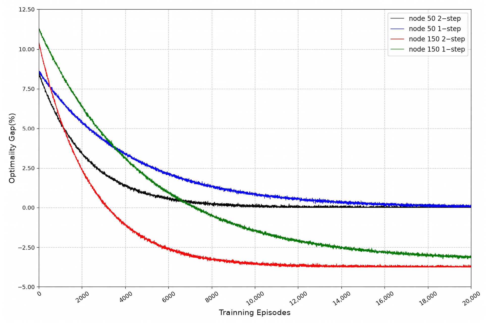
As shown in Figure 8, one-step Q-learning requires many more episodes to converge and settles at a sub-optimal cost, which evaluates the importance of delayed reward propagation. In the constrained SPP, the quality of a current node selection decision is often determined by its long-term influence on future path feasibility and total cost. A one-step temporal difference target may be too myopic to capture such delayed consequences. Therefore, it obtains a worse optimality gap, RPD to CPLEX incumbent and feasibility rate, which indicates that the n-step learning mechanism is more suitable for sequential constrained path construction.

Overall, this ablation study verifies that the proposed E2E_GERL benefits from the combination of the structure2vec-based graph representation, ReLU–Lagrangian penalty constraint embedding, and n-step value learning. The full model achieves the best balance among solution quality, feasibility and efficiency.

5.9. Efficiency Analysis

Because the node representation in E2E_GERL is conditioned on the evolving partial path and resource state, structure2vec embeddings are recomputed after every path extension decision. This design improves state sensitivity but introduces repeated graph encoding cost, which may become relevant on large graphs. We therefore explicitly profile this cost rather than relying solely on aggregate wall-clock measurements.

We instrument the inference pipeline of E2E_GERL and measure the wall-clock cost of every component separately, across seven graph sizes |V| ∈ {30, 50, 100, 200, 600, 800, 1558}. For each test query, the end-to-end online inference time is decomposed as $T_{total}=T_{embed}+T_Q+T_{step}+T_{other}$, where $T_{embed}$ includes all structure2vec forward labels, $T_Q$ denotes Q-network forward labels with candidate action-value evaluation, and the remaining terms capture dynamic feature construction, structural masking, and step updates. Because the number of embedding recomputations equals the number of path extension decisions, we additionally report the average number of decisions $H\left(P\right)$, i.e., the total embedding latency per query. The average embedding latency per decision is ${\overline{T}}_{embed/step}={\displaystyle \frac{T_{embed}}{H\left(P\right)}}$. The proportion of inference time attributable to embedding and Q-network are reported as $R_{embed}={\displaystyle \frac{T_{embed}}{T_{total}}}\times 100\%$ and $R_Q={\displaystyle \frac{T_Q}{T_{total}}}\times 100\%$. The results of the profiling experiment are shown in

Table 10. Inference time decomposition of E2E_GERL.

N	H(P)	Rembed%	RQ%	$\overline{\mathbf{T}}$embed/step (s)	Ttotal (s)
30	5.3	60.32%	38.00%	0.016	0.15
50	7.2	63.43%	35.15%	0.020	0.23
100	8.5	70.86%	28.31%	0.026	0.32
200	10.8	74.92%	24.36%	0.037	0.54
600	13.1	83.54%	16.15%	0.042	0.67
800	15.4	84.41%	15.31%	0.050	0.92
1558	14.5	83.29%	16.25%	0.070	1.23

.

The embedding recomputation is the largest single cost. Shown in the Table 10, structure2vec forward accounts for 60–84% of the per-episode wall-clock time. Even though the embedding must be recomputed at every step, there are still three mitigations keeping the cost tractable. The one is that the edge transformation network ${\mathsf{\varnothing }}_e(·)$ is computed once per episode and cached, so the $K_{\mu }$ propagation steps reuse the cached edge embeddings instead of re-running the two-layer MLP per step. Effective cost per step is $O(K_{\mu }·|E|·d)$ instead of $O(K_{\mu }·|E|·d^2)$. The second one is that the Q-network is batched once per step with the candidate-action set $\mathcal{A}\left(s_t\right)$, so its per-step cost is independent of |V| and only the embedding recomputation depends on |V|. The structure2vec cost scales roughly linearly in |V|, and the cost is $O\left(\right|E|·d)$, not $O\left(\right|V{|}^2·d)$. The third mitigation is that the Lagrangian λ update in Equation (6) drives the agent toward feasible paths quickly, and hence the worst-case recomputation count is rarely reached.

5.10. Experiments on Real-World Instance

To further verify the actual performance of our method, we conduct experiments using both generated data and real-world data, applying the algorithm to a real-world instance for the problem. The real-world instance data come from a logistics company in China, based on which a vast graph is modeled, composed of 1558 nodes and 3253 edges. A summary of the results is shown in

Table 11. Average objective, computing times and RPD to CPLEX incumbent of each method under real-world instance.

	Real-World Instance N = 1558
Method	Obj.	Time (s)	RPD%
CPLEX	292,450	3600	0.00%
RC-BD	258,584	3600	−11.58%
ACO	278,675	3600	−4.71%
L2I	301,106	15.92	2.96%
AM	260,602	65.84	−10.89%
GAT	246,331	5.01	−15.77%
E2E_GERL	202,867	1.23	−30.63%

, where E2E_GERL outperforms all competing baselines.

The experimental results clearly demonstrate that traditional exact algorithms and heuristic algorithms CPLEX, BD, and ACO all reach the 3600 s time limit, and are unable to effectively solve large-scale problems. NCO baselines can solve it with relatively less time, while our algorithm shows high efficiency and accuracy.

To strengthen the real-world evaluation beyond a single routing instance, we construct a multiple O-D pairs experiment. The experiment constructs a fixed set of $K_{OD}=20$ valid origin–destination pairs from the independent 1558-node logistics network. We define $K_{OD}=20$ O-D pairs on the same graph using a greedy spread procedure: We first sample random (origin, destination) pairs and collect those with a directed path from origin to destination, and then iteratively pick the remaining pair. Candidate origin–destination pairs are first screened to ensure directed reachability. We then compute the lexicographic minimum cost and minimum time paths for each candidate pair and retain only non-degenerate pairs satisfying $T_i^t<T_i^c$, so that the routing cost and travel time objectives exhibit a genuine trade-off. For every O-D pair, the time constraint is generated as $T_{max,i}=T_i^t+\delta \left(T_i^c-T_i^t\right),\delta =0.6$. This guarantees the existence of at least one feasible path while excluding the unconstrained minimum cost path from the feasible set. In total, $K_{OD}=20$ O-D constrained routing queries are evaluated. Of these 20 pairs, 5 are training pairs and 15 are hold-out pairs. This split is the standard experimental protocol for assessing generalization in RL agents. The five training O-D pairs are included in both phases so that we can compare in-distribution performance (train O-D) against out-of-distribution performance (hold-out O-D). CPLEX is executed separately for every query. When global optimality is certified, solution quality is reported using certified optimality gap; otherwise, RPD to the time-limited CPLEX incumbent is reported. To account for stochastic training variability, E2E_GERL is trained using 10 random seeds.

The results in

Table 12. Validation of multiple O-D pairs under real-world instance.

Group	Time (s)	RPD%	Fsb%
Train O-D	0.35	−0.27 ± 0.00%	100 ± 0.00%
Hold-out O-D	0.42	−0.24 ± 0.02%	99.14 ± 0.06%
All O-D	0.45	−0.24 ± 0.03%	98.25 ± 0.11%

show that the difference in solution quality and feasibility between the trained O-D pairs and the hold-out O-D pairs is small, which means that the learned policy has captured transferable structural patterns of the logistics network rather than over-fitting to a single origin–destination instance. This is the primary evidence to claim thst E2E_GERL has good generalization ability.

6. Conclusions

This study investigates the constrained SPP, a fundamental resource-constrained routing optimization problem with important applications in transportation, logistics, communication networks, and supply chain decision systems. To overcome the exponential scalability bottlenecks of traditional exact and heuristic algorithms and the feasibility violations inherent in standard NCO, we propose E2E_GERL, an end-to-end graph-embedded reinforcement learning algorithm for the time-constrained SPP. Our approach reformulates the problem as a structure-aware and resource-aware sequential decision-making process, where an agent incrementally constructs a path from the source node to the destination node by evaluating feasible successor nodes under the current partial path state. By synergizing structure2vec graph embeddings with a n-step fitted Q-iteration algorithm, the model successfully captures the long-term structural equivalence of critical graph nodes while effectively propagating delayed constraint feedback. Furthermore, the integration of feasibility action mask and a ReLU-based Lagrangian penalty embedding time constraint violation into the reinforcement learning objective not only guarantees loop-free trajectory construction, but also enables the model to jointly consider cost minimization and time feasibility.

The effectiveness of our proposed method has been demonstrated through experiments. The empirical results demonstrate that E2E_GERL can not only match the optimality of exact algorithms on small-scale instances but also significantly outperform other baselines in both solving accuracy and speed on large-scale instances. Comprehensive ablation studies further confirm that the performance benefits from the joint contribution of structure2vec-based graph representation, ReLU–Lagrangian penalty constraint embedding, and n-step value learning.

Although our proposed algorithm has yielded promising results in solving the SPP with constraints, it is important to note that the existing framework is primarily evaluated on deterministic graphs featuring a single resource constraint. When faced with problems involving multiple or complex constraints, our algorithm begins to exhibit certain limitations. The principal computational bottleneck is the state-dependent graph embedding, which is recomputed after each path extension decision. The profiling experiments therefore quantify this component explicitly rather than relying only on aggregate wall-clock time. The reported results provide evidence of scalability over the graph sizes and sparsity regimes evaluated here, including the real logistics network, but should not be interpreted as guaranteeing unchanged performance on arbitrarily large or substantially denser graphs. These shortcomings have also motivated our future research. In subsequent work, we will attempt to refine the algorithm to handle the SPP with more complex constraints, while also expanding its application to a broader range of combinatorial optimization problems. Related adaptations may also be investigated for constrained orienteering, resource-constrained routing, and other graph-based combinatorial problems in which solutions are built sequentially under cumulative resource limits. Another promising direction is to study E2E_GERL as a fast heuristic or warm-start mechanism for resource-constrained pricing subproblems within larger exact decomposition frameworks. Extension to non-graph or non-sequential combinatorial optimization problems would require more substantial architectural changes and is left for future research.