


Abstract
Real data such as road traffic mortality rates and lifetime observations are often zero-inflated and right-skewed. The zero-inflated two-parameter Rayleigh (ZITR) distribution is employed to model such data in this study. The coefficient of variation (CV) is a statistical measure that is used to quantify the relative dispersion of a population, by comparing the standard deviation with the mean. It is widely used to evaluate variability and facilitate comparisons among datasets with different scales or measurement units. This study develops and evaluates seven methods for constructing confidence intervals for the single CV of the ZITR distribution. Three proposed approaches, including Bayesian Markov chain Monte Carlo (MCMC), Bayesian highest posterior density (HPD), and approximate normal (AN) methods, are compared with three existing approaches: generalized confidence interval (GCI), percentile bootstrap (PB), and bootstrap with standard error (BS). Monte Carlo simulations are employed to assess the efficacy of these methods in terms of expected length (EL) and coverage probability (CP). The simulation results show that the HPD method gives acceptable CP with shorter interval lengths than other methods. Moreover, the proposed methods are illustrated with road traffic mortality rates per 100,000 population collected in January 2026 from the Phichit, Suphan Buri, and Prachuap Khiri Khan provinces in Thailand. The results indicate the applicability of the proposed methods for analyzing zero-inflated and right-skewed data in this real-data example.
Keywords:
resampling; pivotal quantities; generalized confidence interval; prior distribution; highest posterior density; delta method; bayesian credible interval; gibbs sampling MSC:
62F25
1. Introduction
Estimation of population parameters is an important part of statistical inference. A point estimate provides a single summary result. However, it does not account for uncertainty due to the sampling procedure. Interval estimation solves this problem by giving a confidence interval (CI) that includes a range of possible values for the parameter of interest. These intervals explicitly account for variability arising from the sampling process, thereby offering a more comprehensive framework for statistical inference. Therefore, it is important to construct suitable confidence intervals to make reliable statistical inferences [1].
In many practical situations, a large number of zero observations may cause serious problems in statistical analysis, especially when accurate estimation is required and zero outcomes are a natural consequence of the data-generating process. Continuous distributions may produce inaccurate parameter estimates and increased dispersion when applied to datasets containing an excessive number of zero observations, since they are not specifically designed to accommodate exact zeros. Ignoring the presence of excess zeros may lead to unreliable and even misleading inferential results [2,3]. Aitchison [4] proposed a simple framework to address these problems. The observations are represented through a mixed framework consisting of a degenerate component at zero together with a continuous distribution for positive values, thereby improving the ability to accommodate excess zeros in the data. Later, Lambert [5] extended zero-inflated modeling approaches by introducing a systematic method for handling data with more zeros than expected under conventional models.
The Rayleigh distribution is a non-negative continuous distribution defined on the positive real line including zero and is widely applied to describe right-skewed data [6]. However, the standard model has limited flexibility, primarily capturing the degree of skewness without accounting for potential shifts in location. To this end, a two-parameter Rayleigh distribution (TR) was developed with an additional location parameter. The fundamental properties of this generalized form of the distribution were systematically examined in pioneering studies, particularly by Johnson [7]. Statistical inference for TR distribution, particularly in the context of unknown parameter estimation, has received increasing attention in recent years, as reported by Dey [8]. Moreover, numerous works have focused on the development and evaluation of estimators for this distribution to pursue accurate and reliable parameter estimation, as illustrated by Seo [9].
The zero-inflated two-parameter Rayleigh distribution () incorporates an additional parameter, , which corresponds to the probability mass at zero. This construction maintains the capacity of TR to characterize right-skewed behavior in the positive domain, while providing a mechanism to explicitly account for excess zeros in the data. Thus, it offers a flexible framework for modeling datasets characterized by excess zeros and positive continuous observations, making it suitable for applications in many fields, including the analysis of accident-related fatalities, severe disease outcomes, and lifetime data.
The coefficient of variation (CV), defined as the ratio of the standard deviation to the mean, is a unitless measure of relative variability [10]. Although the CV is a function of the mean and variance, direct inference on the CV provides information on variability relative to the mean that cannot be obtained by considering the mean or variance separately. In particular, its dimensionless nature facilitates meaningful comparisons of relative variability across datasets with different scales or measurement units. Thus, it has been extensively used in several different areas. For instance, Kim et al. [11] used the CV to study the patterns of variability in hydrogen-fueled engines, and Gulhar et al. [12] used it to study the fluctuations of smoking prevalence in the tobacco control settings. A considerable amount of studies have also been devoted to the construction of confidence intervals for CV. For instance, for the CV under the normal distribution, Vangel [13] proposed confidence intervals. Curto and Pinto [14] developed statistical tests for comparing two coefficients of variation in the non-independent and non-identically distributed case. For standard continuous distributions without zero inflation, inference on the coefficient of variation has been extensively studied in classical statistical settings. La-ongkaew [15] examined Bayesian credible intervals for the Weibull distribution. Sangnawakij [16] discussed confidence interval methods for the population mean and CV of the two-parameter exponential distribution.
In contrast, several studies have considered estimation of CV for distributions with a probability mass at zero. For instance, Yosboonruang [17] examined Bayesian credible intervals for CV of a zero-inflated lognormal distribution. More recently, Janthasuwan [18] investigated confidence interval procedures for the CV under the Delta–Birnbaum–Saunders distribution, while Khumpasee et al. [19] proposed confidence interval methods for CV in delta inverse Gaussian distributions.
The estimation of a single CV constitutes an important inferential problem because it quantifies relative variability within a population and provides a basis for subsequent comparative inference, such as the difference and ratio of CVs between populations. Therefore, reliable interval estimation for a single CV remains important, particularly for complex distributions involving excess zeros.
The present study is closely related to a companion manuscript that investigates interval estimation of the difference and ratio of CVs between two independent populations under the ZITR distribution. Nevertheless, the objectives and inferential problems addressed in the two studies are fundamentally different. While the companion manuscript focuses on comparative inference based on the difference and ratio of CVs between two populations, the present study addresses direct interval estimation of a single population CV. Thus, the two studies answer different inferential questions: the former assesses relative variability between populations, whereas the present study quantifies and provides uncertainty assessment for relative variability within a population.
Although the interval estimation techniques considered in this study are established methods in the statistical literature, their application to the ZITR distribution is not a direct substitution. The CV of the ZITR distribution has a different functional form from those of previously studied zero-inflated models because both the zero-inflation parameter and the two-parameter Rayleigh distribution jointly determine its mean and variance. Consequently, likelihood-based inference, Bayesian posterior construction, and interval estimation procedures must be formulated specifically for the ZITR model. To the best of our knowledge, confidence interval estimation for the CV under the ZITR distribution has not previously been investigated. Therefore, the inferential contribution of this study lies in developing the framework required for interval estimation of the CV under the ZITR distribution, whereas the interval estimation algorithms themselves are adaptations of existing methodologies.
Methodologically, this study investigates and compares several interval estimation methods for the coefficient of variation under the ZITR distribution. Specifically, Bayesian MCMC and HPD credible intervals and the approximate normal (AN) method are considered and compared with three standard methods, namely the generalized confidence interval (GCI), percentile bootstrap (PB), and bootstrap based on standard errors (BS) methods. Their performances are comprehensively evaluated through Monte Carlo simulations in terms of coverage probability (CP) and expected length (EL).
2. Materials and Methods
Let the positive observations in the population be suitably modeled by a continuous distribution. The population consists of both positive value and zeros observations, where the probability of observing a zero is denoted by , with . A random sample of size n is partitioned into two groups: zero observations, denoted by , and positive observations, denoted by , such that .
This study assumes that the positive observations follow a two-parameter Rayleigh distribution (TR). Consider a random sample from the zero-inflated two-parameter Rayleigh distribution, written as , where is the scale parameter, is the location parameter, and is the zero-inflation probability. The corresponding probability density function is
The likelihood function based on the observed data is
Hence, the log-likelihood function is
Calculating the derivative of the log-likelihood about yields
Equating the score equation to zero yields
Differentiating with respect to gives
Since the score equation for is non-linear, no closed-form solution exists. Therefore, is obtained numerically using the uniroot function in R version 4.4.1. The search interval is defined as
where with s denoting the sample standard deviation of the positive observations. The convergence tolerance is set to , with a maximum of 20 iterations. Therefore, the coefficient of variation (CV) can be expressed as
The estimator of the CV is then obtained by substituting the corresponding MLEs of the parameters into the following expression:
2.1. Proposed Method
This study discusses ways to create credible intervals and confidence intervals for estimating the parameter CV for the ZITR distribution. The proposed approaches include Bayesian Markov Chain Monte Carlo (MCMC), Bayesian highest posterior density (HPD), and approximation normal (AN) procedures. They have been chosen due to their adaptable and computationally efficient characteristics in intricate distributional scenarios. Appendix B contains the theoretical formulation of the AN technique.
2.1.1. Bayesian Markov Chain Monte Carlo (MCMC)
The CV parameter is estimated for data assumed to follow the distribution inside a Bayesian framework. According to Bayes’ theorem [20,21], the posterior distribution of the unknown parameters is determined by revising the prior distributions with the information available in the observed data. Because the resulting posterior distribution is analytically intractable, posterior samples are generated using MCMC methods, specifically Gibbs sampling, and are subsequently used to make inferences about .
Here, we use informative priors to incorporate available prior information while maintaining posterior propriety [8]. The prior distributions are selected according to the characteristics and the support of the corresponding parameters. Specifically, the Gamma, Uniform, and Beta priors are provided to the scale parameter , the location parameter , and the zero-inflation parameter , respectively.
In the R version 4.4.1 environment, the R2OpenBUGS package version 3.2-3.2.1 is employed to conduct all Bayesian analyses. The Gibbs sampling algorithm, which is implemented in OpenBUGS version 3.2.3, is employed to generate posterior samples.
The convergence and mixing performance of the MCMC algorithm were assessed before conducting Bayesian inference. In this study, a single Markov chain was generated with 20,000 iterations, where the first 5000 iterations were discarded as burn-in. Therefore, the remaining 15,000 posterior samples were retained for estimating and constructing the corresponding Bayesian credible intervals. The convergence of the Markov chain was examined using trace plots and autocorrelation function (ACF) plot. The trace plots demonstrate that the sampled chains move consistently around their posterior averages, exhibiting no discernible trends or non-stationary characteristics, indicating adequate convergence. In addition, the ACF plots show a rapid decay of autocorrelation toward zero, indicating weak serial dependence among posterior samples and adequate mixing performance. The corresponding diagnostic plots are provided in Figure A1 and Figure A2 in the Appendix A.
The following describes the procedure for constructing two-sided Bayesian credible intervals for based on these MCMC posterior samples.
In this work, the credible interval for CV of the is computed using the Bayesian MCMC technique, following the steps described in Algorithm 1.
| Algorithm 1: Bayesian Markov Chain Monte Carlo |
|
2.1.2. Bayesian Highet Posterior Density (HPD)
The Bayesian HPD technique defines an interval derived from the posterior distribution that encompasses the most likely parameter values while reducing the interval’s length [22]. In this study, HPDs are used to estimate CV parameter, denoted by . The computation of these intervals is carried out using the R package HDInterval. Accordingly, the HPD criterion yields a two-sided Bayesian credible interval for , which is denoted as
In this study, the credible interval for CV of the is calculated using Bayesian HPD approach, following the steps of Algorithm 2.
| Algorithm 2: Bayesian Highet Posterior Density |
|
2.1.3. Approximate Normal (AN)
The asymptotic properties of MLE for the coefficient of variation are established using the Delta method. Let
denote the coefficient of variation of the ZITR distribution, and let
be its MLEs. The following results are established under the standard regularity conditions for MLEs. Specifically, it is assumed that the true parameter values satisfy
the log-likelihood function
is twice continuously differentiable with respect to the model parameters, and the corresponding Fisher information exists and is finite and positive. Under these conditions, the MLEs are consistent, i.e.,
and are asymptotically normally distributed. Furthermore, the coefficient of variation
is continuously differentiable with respect to , , and . Therefore, the first-order Delta method can be applied. Specifically, by a first-order Taylor expansion of around the true parameter values ,
which forms the basis of the first-order Delta method for deriving the asymptotic distribution and variance of . The detailed derivation is provided in Appendix B. The following theorem establishes the asymptotic distribution of .
Theorem 1.
Asymptotic normality of the coefficient of variation estimator.
Consider a random sample from the ZITR distribution. Let
denote CV of the ZITR distribution. Then, as ,
where denotes the asymptotic variance of . An explicit estimator of is derived using the Delta method and is presented in Theorem 2, with the detailed derivation provided in Appendix B.
Theorem 2.
Asymptotic variance of the CV estimator.
Under the conditions of Theorem 1, the asymptotic variance of is given by
The above expression is obtained using the Delta method by applying a plug-in estimator to the asymptotic variance derived in Theorem 1. The detailed proof is provided in Appendix B. Based on the approximation normal, the confidence interval for is .
where represents the upper critical value from the standard normal distribution, and denotes the estimated variance of derived via the Delta method.
2.2. Standard Method
The three suggested techniques were evaluated against three conventional approaches, namely the generalized confidence interval (GCI), the percentile bootstrap (PB), and the bootstrap method using standard error (BS) to assess their efficacy.
2.2.1. Generalized Confidence Interval (GCI)
An alternative framework for parameter estimation was developed by Krishnamoorthy et al. [23], who constructed pivotal quantities (GPQ) for the TR distribution. GCI method for interval estimation has been suggested by many authors and was introduced by Weerahandi [24] as a flexible approach to constructing confidence intervals when nuisance parameters are present.
A function is referred to as GPQ for interval estimation when the parameter of interest is denoted by , the nuisance parameters are represented by , and the following conditions hold:
- No unknown parameters are present in the probability distribution of .
- Evaluating at the observed sample values yields a quantity that depends only on the parameter of interest , while the nuisance parameters are eliminated from the resulting expression.
The methodology was further extended by Wu and Hsieh [25] who applied variance-stabilizing transformations (VSTs) to construct GPQ for the proportion of zero observations. Building upon this framework, GPQ for CV is defined as follows
The confidence interval for derived via GCI approach is expressed as
GCI for the coefficient of variation of is obtained following the procedure described in Algorithm 3.
2.2.2. Percentile Bootstrap (PB)
The bootstrap is a simulation-based technique established by Efron [26] that estimates the sampling distribution of a data set by repeated resampling. Bootstrap samples are generated by repeatedly sampling with replacement from the original dataset. This technique, when repeated, produces a series of bootstrap estimates of , from which an empirical distribution is derived. PB for is defined based on the empirical quantiles of the ordered bootstrap estimates as
In this expression, and are the empirical quantiles of order and of the bootstrap samples. The procedure for the calculation of this is given in Algorithm 4.
| Algorithm 3: Generalized Confidence Interval |
|
| Algorithm 4: Percentile bootstrap |
|
2.2.3. The Bootstrap with Standard Error (BS)
BS presents an alternative to the usual interval estimation processes without the need for an explicit analytical representation of the standard error. The estimator’s variability is derived directly from the resampling method. In this context, several bootstrap samples are generated, and the empirical distribution derived from this procedure is used to estimate the standard error, which will be utilized to create confidence intervals. This method is especially beneficial in scenarios with a restricted sample size or where the theoretical variance cannot be derived in a closed form. Let , where , represent the bootstrap estimates of the parameter of interest derived from B resamples. The corresponding standard error is determined as the sample standard deviation of . Thus, the two-sided confidence interval for , derived from the bootstrap standard error, may be articulated as
where is the standard error estimate from resampling, and is the upper -quantile of the standard normal distribution. The methodology for computing this is outlined in Algorithm 5.
| Algorithm 5: Bootstrap with standard error |
|
3. Results
Monte Carlo simulation was employed to assess the effectiveness of confidence intervals for CV associated with the distribution at a nominal confidence level of 0.95. Coverage probability (CP) and expected length (EL) were used as performance criteria. An efficient approach should yield CPs that are at least as large as the nominal confidence level together with comparatively narrow interval widths. For each replication, random samples were generated from the ZITR distribution under the specified parameter settings . The coefficient of variation () was subsequently estimated, and the corresponding confidence intervals were constructed using each competing method. For each interval, it was determined whether the true CV value was contained within the interval. The CP was then estimated as the proportion of intervals covering the true CV, whereas the EL was calculated as the average interval width across all replications. Specifically, the CP and EL were computed as
and
where M denotes the total number of Monte Carlo replications, and are the lower and upper confidence limits obtained from the mth replication, respectively, is the true coefficient of variation, and is the indicator function that takes the value 1 if the true CV is contained within the interval and 0 otherwise.
For each parameter configuration, m = 1000 Monte Carlo simulations were generated for all considered methods. In the bootstrap procedures, b = 1000 bootstrap resamples were drawn within each replication, whereas the generalized confidence interval method was implemented using q = 2500 repetitions. For the Bayesian approaches, both MCMC and HPD methods were based on t = 20,000 posterior simulations, with the first c = 5000 iterations discarded as burn-in samples.
The simulation settings were specified with and 1, and 1, and , , and , while the sample sizes considered were and 200.
Table 1, Table 2, Table 3, Table 4, Table 5 and Table 6 summarize the corresponding CP and EL results, which are illustrated in Figure 1, Figure 2, Figure 3 and Figure 4.
Table 1.
Simulation results for 95% confidence intervals of CV under the distribution with fixed and .
Table 2.
Simulation results for 95% confidence intervals of CV under the distribution with fixed and .
Table 3.
Simulation results for 95% confidence intervals of CV under the distribution with fixed and .
Table 4.
Simulation results for 95% confidence intervals of CV under the distribution with fixed and
Table 5.
Simulation results for 95% confidence intervals of CV under the distribution with fixed and .
Table 6.
Simulation results for 95% confidence intervals of CV under the distribution with fixed and .
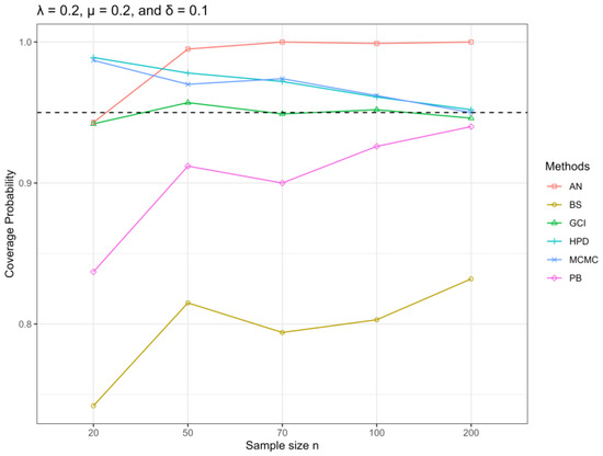
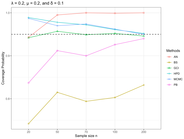
Figure 1.
CPs for the confidence intervals of the coefficient of variation under the were assessed for the parameter configuration , , and . The techniques were considered appropriate when the corresponding CP reached at least 0.95, as indicated by the dashed reference line in the figure representing the nominal confidence level, thereby reflecting adequate coverage of the true parameter. The findings shown in the figure indicate that the HPD, MCMC, and AN techniques consistently yielded CP values at or above the nominal level. This signifies that these methods provide dependable interval estimations for this context.
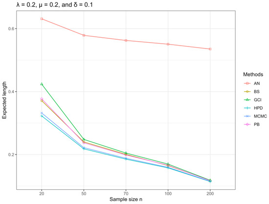
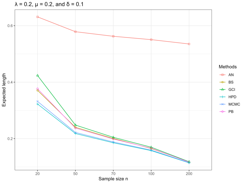
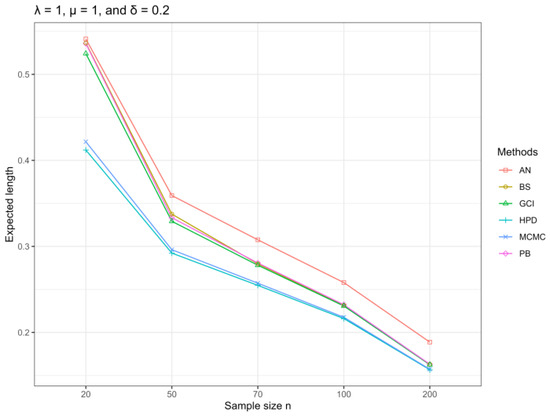
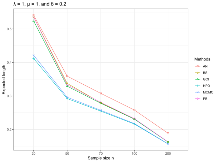
Figure 2.
ELs of the confidence intervals for the coefficient of variation under the were analyzed for the parameter configuration , , and . This study focused on approaches that yielded CPs at or above the nominal confidence level of 0.95, while also generating the smallest interval lengths. In this context, the HPD, MCMC, and AN methodologies fulfilled the CP requirement. The HPD approach yielded the shortest EL, signifying a more efficient interval estimation under the specified parameters.
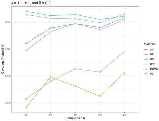
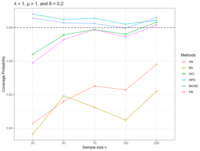
Figure 3.
CPs of the confidence intervals for the coefficient of variation under the were assessed for the parameter configuration , , and . The techniques were considered appropriate when the corresponding CP reached at least 0.95, as indicated by the dashed reference line in the figure representing the nominal confidence level, thereby reflecting adequate coverage of the true parameter. The findings indicate that the majority of the methods, especially HPD and MCMC, yielded CP values near or beyond the nominal level, indicating that these techniques provide dependable interval estimates in this context.
Figure 4.
ELs of the confidence intervals for the coefficient of variation under the distribution were assessed for the parameter configuration , , and . The comparison emphasized approaches that attained CPs around or above the nominal threshold of , while concurrently yielding reduced interval lengths. In this context, HPD and MCMC methodologies satisfied the CP criteria. According to these situations, the HPD approach yielded the shortest EL, suggesting a more effective interval estimate.
The CPs of CV are generally close to the nominal confidence level of 0.95, as shown by Table 1, Table 2, Table 3, Table 4, Table 5 and Table 6 and Figure 1, Figure 2, Figure 3 and Figure 4. The Bayesian MCMC, Bayesian HPD, and GCI methods are robust in the considered scenarios, even for small sample size cases. However, the AN and BS methods show undercoverage in several situations, particularly for small sample sizes. The problem for AN method is more severe when the location parameter is relatively large compared to the scale parameter, but its coverage performance improves with increasing sample size. The PB method also improves gradually with increasing sample size; CPs get closer to the nominal level. On the other hand, the BS method tends to produce shorter ELs but with lower CPs, especially in small sample situations. All methods show that larger sample sizes tend to produce shorter ELs, which indicates the improvement of the estimation precision. In summary, in terms of both CP and EL, the HPD method has the most desirable performance characteristics by preserving acceptable CPs and relatively shorter interval lengths.
4. Application
The proposed confidence interval procedures under the are shown with the use of real data in the application section of this study. The dataset exhibits a zero-inflated configuration, including both zero observations and positive values that adhere to a two-parameter Rayleigh distribution. The information utilized in this examination consists of traffic mortality rates per 100,000 individuals, sourced from the road traffic fatality statistics provided by the Thai Road Safety Center (https://www.thairsc.com/) (accessed on 10 June 2026) and the relevant district population figures acquired from the Bureau of Registration Administration, Department of Provincial Administration, Ministry of Interior, Thailand (https://stat.bora.dopa.go.th/stat/statnew/statMenu/newStat/home.php) (accessed on 10 June 2026). Following the definition of the World Health Organization (WHO), the road traffic mortality rate is defined as the number of road traffic deaths per 100,000 population. Accordingly, the mortality rate for each district was calculated as
where represents the road traffic mortality rate for district i, represents the number of road traffic fatalities, and represents the corresponding district population. The statistics include the road traffic fatality rates per 100,000 people for January 2026, categorized by district in the provinces of Phichit, Suphan Buri, and Prachuap Khiri Khan, Thailand. The data that were observed are shown in Table 7. The Akaike Information Criterion (AIC) and the Bayesian Information Criterion (BIC) are employed to select an appropriate model for the real-data analysis based on the positive observations. These criteria are used to determine which candidate distribution provides the best fit to the data. The model exhibiting the lowest AIC and BIC values is considered the optimal depiction of the data [27,28].
Table 7.
Road traffic mortality rates per 100,000 population for districts in the Phichit, Suphan Buri, and Prachuap Khiri Khan provinces.
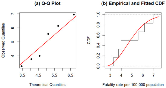
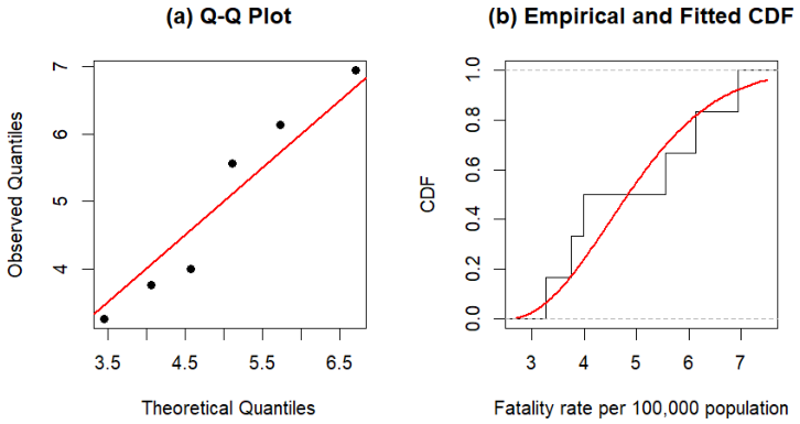
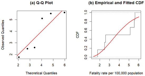
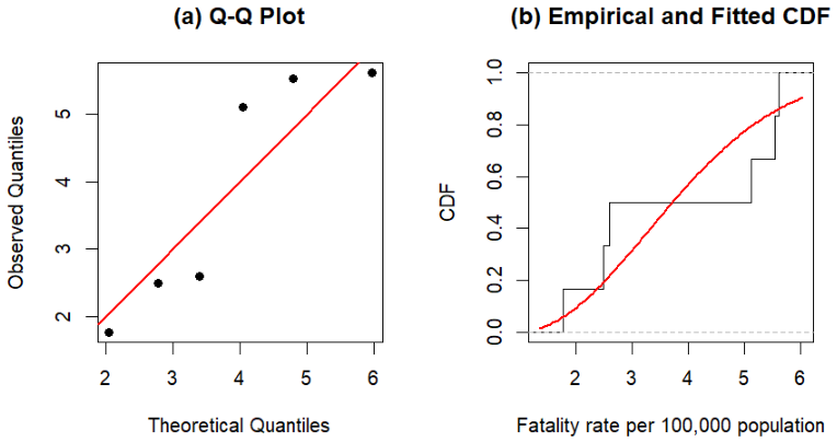
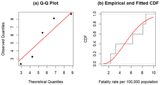
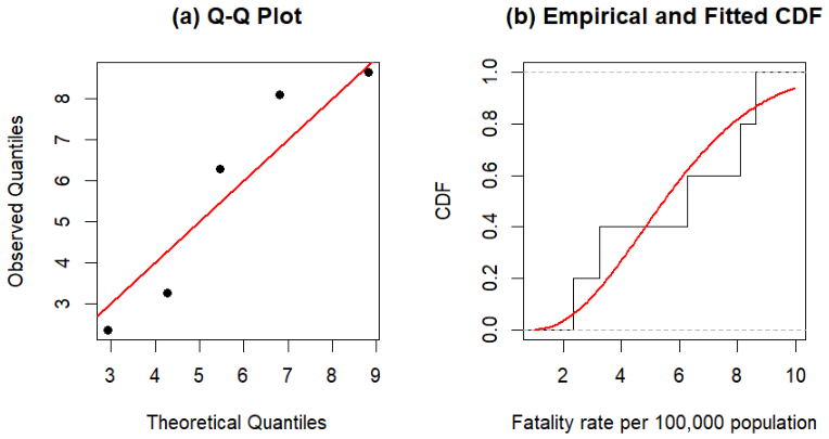
The AIC and BIC values of the candidate models used to evaluate the suitability of the distributions for the data are presented in Table 8, Table 9 and Table 10. The findings suggest that the TR distribution offers the most accurate representation of the road traffic death rate data collected in January 2026 from the Phichit, Suphan Buri, and Prachuap Khiri Khan provinces in Thailand. Figure 5, Figure 6 and Figure 7 display Q–Q plots and the comparison of the empirical and the fitted CDFs for the three provinces, which lends further support to the suitability of the TR distribution. The observed quantiles are close to the theoretical quantiles and the fitted CDFs are in good agreement with the empirical CDFs showing that the TR distribution is appropriate for the observed road traffic fatality rate data. The MLEs of the parameters under the model, together with the corresponding estimate of the CV, are presented in Table 11. Summary statistics of the posterior of the coefficient of variation () under the ZITR model are presented in Table 12. For all three provinces, the posterior mean and posterior median are similar, suggesting symmetric posterior distributions. The posterior means are reasonably close to the corresponding maximum likelihood estimates reported in Table 11, indicating general agreement between the Bayesian and frequentist point estimates. Table 13, Table 14 and Table 15 present the confidence intervals for the CV obtained from the proposed methods under the model. The results indicate that the shortest interval length is obtained by the HPD method, followed by the MCMC, AN, BS, PB, and GCI methods. Based on the simulation results, considering both the CP and EL, the HPD approach appears to be the most appropriate method for constructing confidence intervals for the coefficient of variation when the underlying population follows the distribution.
Table 8.
Model comparison based on AIC and BIC for road traffic mortality rates per 100,000 population across districts in Phichit Province, January 2026.
Table 9.
Model comparison based on AIC and BIC for road traffic mortality rates per 100,000 population across districts in Suphan Buri Province, January 2026.
Table 10.
Model comparison based on AIC and BIC for road traffic mortality rates per 100,000 population across districts in Prachuap Khiri Khan Province, January 2026.
Figure 5.
Q–Q plot and comparison of the empirical and fitted cumulative distribution functions (CDFs) for the positive observations under the fitted two-parameter Rayleigh distribution using the road traffic fatality rates per 100,000 population in Phichit Province, Thailand, for January 2026.
Figure 6.
Q–Q plot and comparison of the empirical and fitted cumulative distribution functions (CDFs) for the positive observations under the fitted two-parameter Rayleigh distribution using the road traffic fatality rates per 100,000 population in Suphan Buri Province, Thailand, for January 2026.
Figure 7.
Q–Q plot and comparison of the empirical and fitted cumulative distribution functions (CDFs) for the positive observations under the fitted two-parameter Rayleigh distribution using the road traffic fatality rates per 100,000 population in Prachuap Khiri Khan Province, Thailand, for January 2026.
Table 11.
MLEs of the ZITR model parameters and the corresponding estimated coefficient of variation for the road traffic mortality rates per 100,000 population in the Phichit, Suphan Buri, and Prachuap Khiri Khan provinces in January 2026.
Table 12.
Summary statistics of the posterior distribution for the coefficient of variation () under the ZITR model.
Table 13.
Estimates of the confidence interval for the CV parameter under : January 2026 mortality rates per 100,000 population in Phichit province.
Table 14.
Estimates of the confidence interval for the CV parameter under : January 2026 mortality rates per 100,000 population in Suphan Buri province.
Table 15.
Estimates of the confidence interval for the CV parameter under : January 2026 mortality rates per 100,000 population in Prachuap Khiri Khan province.
The sample sizes of the provincial datasets are relatively small, which might affect the performance of some interval estimation approaches for the CV. In particular, the AN and GCI approaches might have lower coverage performance under the small sample condition, as indicated in the simulation study. Therefore, the interval estimates for the CV obtained from these approaches should be interpreted with caution. The performance of the proposed interval estimation approaches was systematically evaluated through the simulation study, while this practical application aims to demonstrate their implementation for the CV under the ZITR distribution using real-world data.
5. Discussion
The results obtained in this study demonstrate that, across most considered scenarios, the HPD approach outperforms the PB, BS, GCI, AN, and Bayesian MCMC methods in estimating interval bounds for the coefficient of variation under . The main advantage is that it can produce shorter interval lengths while maintaining satisfactory coverage probability.
The HPD method generates shorter interval lengths than the percentile bootstrap method, probably due to the different inferential frameworks on which the two approaches are based. The posterior distribution of CV, which is a combination of the information in the likelihood function and the prior distribution, is used to estimate the HPD interval. HPD interval will select the region of highest posterior density and will tend to give a tighter interval if the posterior distribution is concentrated enough. On the other hand, PB is based on the empirical distribution of bootstrap estimates that may be more variable particularly for small sample sizes leading to wider interval estimates.
However, the GCI and MCMC methods also showed satisfactory performance. Both methods maintained CPs consistently close to or above the nominal confidence level. Although they did not achieve the minimum expected lengths, they provided a reasonable balance between interval width and coverage probability, even for small sample sizes.
In some situations, in particular when the sample size is small and the location parameter is large relative to the scale parameter, the AN method showed considerable undercoverage. This is explained by the use of a first-order Taylor expansion and the asymptotic normality of the estimator. Under such circumstances, the asymptotic approximation may not sufficiently reflect the sampling distribution of the CV, which is a non-linear function of the model parameters. As a result, the delta method based estimates of the variance may be underestimated, leading to confidence intervals that are too narrow and demonstrate undercoverage. With increasing sample size, the asymptotic assumptions become more valid, resulting in improved coverage probabilities. Therefore caution is needed in the application of AN method with small sample sizes, especially when the location parameter is large in comparison to the scale parameter.
Also, the use of AN and GCI methods to real data with small sample sizes needs to be taken care of, as the coverage performance of these methods can degrade in such conditions. This is particularly important for the provincial data used in this study, which has a relatively small number of observations.
These results are consistent with our previous work on interval estimation of the mean and variance parameters of ZITR. In particular, Kijsason et al. ([29,30]) found that Bayesian-based approaches, in particular the HPD interval, performed competitively by providing reasonable coverage probabilities with relatively shorter interval lengths compared to some existing methods. The similar behavior observed in the present study indicates that the effectiveness of the HPD approach can be extended from direct parameter estimation, such as the mean and variance, to the CV of the ZITR distribution. However, unlike the mean and the variance, the CV is a non-linear function of the location and scale parameters. This makes the interval estimation more difficult, since the transformation of the parameter introduces additional uncertainty.
One limitation of the Bayesian procedures is their higher computational cost due to the MCMC sampling scheme. Although the Bayesian HPD method demonstrated competitive statistical performance in terms of coverage probability and expected length, its practical implementation requires longer computation times and greater computational resources than the competing frequentist methods.
Overall, the performances of the frequentist procedures, particularly the PB and AN methods, improved as the sample size increased, reflecting the enhanced accuracy of their large-sample approximations.
The results obtained in this study demonstrate that, across most of the investigated scenarios, the HPD method provides the best overall performance compared with the other considered methods. Although the HPD approach requires higher computational time due to the Bayesian framework, it is preferable when accurate interval estimation is required. In particular, the HPD method generally produces shorter interval lengths while maintaining satisfactory coverage probabilities. These findings indicate that the HPD method offers an appropriate balance between interval precision and coverage accuracy under the investigated settings.
6. Conclusions
In this study, we investigate interval estimation of the coefficient of variation (CV) under the ZITR distribution using several established interval estimation methods adapted to this model. Only a limited set of parameter configurations was considered, in which the scale and location parameters were varied to reflect different degrees of skewness and changes in the minimum observed values. Six interval estimation methods were considered: three proposed methods (Bayesian MCMC, HPD, and AN) and three standard methods (GCI, PB, and BS). Their performances were evaluated through a Monte Carlo simulation study.
In addition, the proposed methods were illustrated using three real datasets on road traffic mortality rates per 100,000 populations in the provinces of Phichit, Suphan Buri, and Prachuap Khiri Khan in January 2026. The empirical results were generally consistent with the simulation findings, with the HPD method often producing the shorter interval estimates across the datasets. The simulation results also showed that the Bayesian MCMC method achieved performance comparable to that of the HPD method under some parameter settings. Overall, for the simulation scenarios and real-data applications considered in this study, the HPD method generally provided the shorter interval estimates while maintaining satisfactory coverage probability. Therefore, the HPD method can be regarded as a favorable choice for interval estimation of the CV under the ZITR distribution within the investigated settings.
One limitation of the proposed methodology is that at extreme levels of zero-inflation or with very small sample sizes its performance may be compromised. Where the proportion of zero observations is very large, the information available for estimating the parameters of the positive component may be limited. This may reduce the stability of the estimator of the CV and the associated interval estimates. Likewise, very small sample sizes can result in less reliable parameter estimation and interval construction. The proposed methods were found to perform satisfactorily for the scenarios investigated, although further investigations with more extreme levels of zero-inflation and smaller sample sizes would provide further insights in their robustness.
Future research might extend the proposed framework of confidence interval to more complex data structures. In particular, the proposed methods could be further explored for the case of censored data, right and left censored observations, which are often encountered in reliability engineering and survival analysis. Moreover, it would be interesting to extend the proposed methodology to other zero-inflated lifetime distributions. These extensions would extend the scope of the proposed methods of confidence interval and provide more flexible tools for the analysis of zero-inflated lifetime data encountered in practical applications.
Author Contributions
Conceptualization, S.K. and S.-A.N.; Methodology, S.K. and S.N.; software, S.-A.N. and S.N.; validation, S.-A.N. and S.N.; formal analysis, S.K.; investigation, S.K. and S.-A.N.; resources, S.-A.N. and S.N.; data curation, S.K.; writing—original draft preparation, S.K. and S.N.; writing—review and editing, S.-A.N. and S.N.; visualization, S.K.; supervision, S.-A.N.; project administration, S.K. and S.N.; funding acquisition, S.-A.N. All authors have read and agreed to the published version of this manuscript.
Funding
This research budget was allocated by the National Science, Research, and Innovation Fund (NSRF) and King Mongkut’s University of Technology North Bangkok (Project no. KMUTNB- FF-69-B-06).
Data Availability Statement
The data presented in this study are openly available in Thai Road Safety Culture Data Center at https://www.thairsc.com (accessed on 28 April 2026).
Acknowledgments
The authors would like to acknowledge King Mongkut’s University of Technology North Bangkok for its support and for providing the necessary facilities and resources that contributed to the successful completion of this research. The authors also sincerely thank the editor and reviewers for their valuable comments, constructive suggestions, and careful evaluation of this manuscript, which have greatly contributed to improving the quality and presentation of this work. During the development of this manuscript, the authors utilized ChatGPT (OpenAI, GPT-5.5) and Grammarly Pro as language assistance tools to improve English expression, grammar, and overall readability. All AI-assisted suggestions were carefully reviewed, revised where appropriate, and verified by the authors, who remain fully responsible for the accuracy and integrity of the published content.
Conflicts of Interest
The authors declare no conflicts of interest.
Abbreviations
The following abbreviations are used in this manuscript:
| CP | Coverage probability |
| EL | Expected length |
| AIC | Akaike information criterion |
| BIC | Bayesian information criterion |
| MCMC | Bayesian Markov chain Monte Carlo credible interval |
| HPD | Bayesian highest posterior density credible interval |
| AN | Approximate normal |
| GCI | Generalized confidence interval |
| PB | Percentile bootstrap |
| BS | Bootstrap method with standard error |
Appendix A
This analysis employed Bayesian methodologies to provide reasonable ranges for CV. Under the baseline prior specification, the analysis concentrated on the convergence and mixing characteristics of the Bayesian technique. The prior distributions were defined as , , and . The MCMC technique was applied using a single Markov chain with 20,000 iterations, where the first 5000 iterations were discarded as burn-in, resulting in 15,000 posterior samples available for Bayesian inference.
Figure A1 and Figure A2 contain the trace plots and autocorrelation function (ACF) plots for the MCMC samples, which are used to evaluate the convergence and mixing behavior. The Markov chains lack apparent trends or non-stationary patterns, as evidenced by the trace plots, which demonstrate that they fluctuate around their posterior means. In addition, the ACF plots demonstrate that the autocorrelations rapidly diminish to zero in the initial delays, suggesting that the chains are adequately mixed, and there is minimal serial dependency. Diagnostic results verify that the posterior samples obtained are sufficient for additional Bayesian inference.
In addition, a previous sensitivity analysis was performed to study the robustness of the Bayesian interval estimators to different choices of prior hyperparameters. Three different prior specifications with different degrees of concentration were considered to study the sensitivity of the Bayesian methods’ performance in terms of CP and EL to the prior assumptions. The results of this analysis provide further evidence for the robustness and reliability of Bayesian estimation procedures under different prior settings.
Figure A1.
Trace plots of the MCMC chains for the CV.
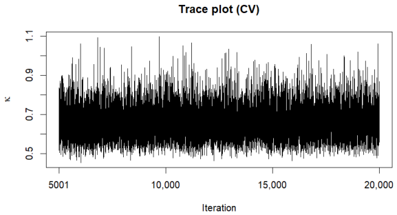
Figure A2.
ACF graphs of the MCMC samples for the CV.
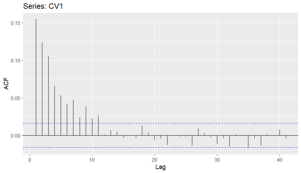
Table A1.
Hyperparameter settings of prior distributions for the sensitivity analysis.
The prior configurations summarized in Table A1 represent different levels of prior information. Specification S1 serves as the baseline prior used throughout the simulation study and real-data application, whereas S2 and S3 correspond to progressively less informative prior settings. The prior distribution of was kept unchanged in all scenarios to isolate the effects of prior choices for the scale and zero-inflation parameters.
The previous sensitivity study used a subset of simulated scenarios with a sample size of , maintaining the location parameter at .
For each prior configuration, the performance was evaluated using the CP and EL of the 95% MCMC and HPD credible intervals under the selected simulation scenarios. The results of the prior sensitivity analysis are summarized in Table A2.
The results indicate that the CP and EL of the Bayesian credible intervals for CV under the ZITR distribution, as determined by the MCMC and HPD methods, remained very consistent across various prior specifications. The variations in CP and EL among the three previous configurations were minimal, suggesting that the posterior inference was quite resilient to different prior assumptions. This stability is crucial for the suggested Bayesian interval estimators, indicating that the resultant credible intervals are not heavily reliant on a specific prior specification.
The prior specification S1, which was implemented in the primary simulation study and real-data application, continues to be a reasonable baseline option, as indicated by the previous sensitivity analysis. Despite the evaluation of several prior configurations, the efficacy of the Bayesian credible intervals for the CV, CP, and EL, remained mostly unchanged. Consequently, the use of prior specification S1 yields consistent and dependable interval estimation outcomes within the examined contexts.
Table A2.
CP and EL of the Bayesian credible intervals for the CV under different prior specifications.
Appendix B
The variance approximation for is developed in this appendix using the delta technique. Let , where CV for is defined as
where and represent the mean and variance of the distribution, respectively. By conducting a first-order Taylor expansion of around the true parameter values , the delta method approximation is obtained. These values are expressed as follows:
Consequently, the variance of can be estimated as follows:
The following is the derivation of the partial derivatives of g(,,):
For illustration, the derivation of the partial derivative with respect to is provided. Since
where and are functions of the model parameters , , and , the partial derivative with respect to can be obtained by applying the quotient rule as follows.
The first term can be obtained as
where
Moreover,
Therefore,
The remaining partial derivatives with respect to and can be obtained similarly.
and
Therefore,
According to Dey et al. [8], the asymptotic covariance matrix of MLEs for the TR can be obtained from the inverse Fisher information matrix. Based on their results, the asymptotic variances of and are given by
and
These asymptotic variance expressions are incorporated into the delta-method procedure for constructing the AN for CV. Thus,
So, an estimate of defined as is expressed as
Appendix C
This appendix presents the computational time required by each interval estimation method considered in the simulation study. The computational time was measured in seconds using the proc.time() function in R under the same computing environment for all methods. All computations were performed on a computer equipped with a 13th Gen Intel Core i7-13650HX processor (2.60 GHz) and 32 GB of RAM.
Table A3 summarizes the average computational time of each method for selected simulation scenarios. The reported times are the average execution times obtained from 1000 Monte Carlo simulation replications. Specifically, the results are presented for sample sizes of and to illustrate the effect of sample size on computational efficiency. The location parameter was fixed at , while various combinations of the scale parameter and the zero-inflation parameter were considered. These selected scenarios provide an overall comparison of the computational efficiency of the competing interval estimation methods.
The AN approach necessitates the least computing duration among all examined interval estimation techniques, exhibiting execution durations almost at zero seconds in all case, as seen in Table A3. This is unsurprising, given that the AN approach relies on an analytical approximation and does not need iterative sampling or resampling techniques. The GCI technique has a small computational time, but its computational cost slightly increases with sample size due to the numerical calculations.
The Bayesian MCMC and HPD methods are more computationally expensive than the other methods due to the iterative procedure of the posterior sampling and the construction of the HPD intervals. Their computational times vary from about 3 s for n = 20 to about 5 s for n = 200. The difference of computational time between the MCMC and HPD techniques is negligible, which shows that the extra computations to generate the HPD intervals based on the posterior sample are minor.
The bootstrap-based methods PB and BS require moderate computational time. The computational costs increase with the sample size because of the repeated implementation of the resampling and parameter estimation procedures. The overall results on computing time suggest a trade-off between computational efficiency and statistical effectiveness.
Although the Bayesian MCMC and HPD approaches are more computationally demanding than the other approaches, their acceptable coverage probabilities and shorter expected lengths observed in the simulation study make the extra computational cost justifiable. In particular, the HPD method provides a good balance between computational cost and interval estimation performance, as it generally maintains coverage probabilities close to the nominal level while producing shorter expected lengths. Therefore, the HPD method can be considered a practical choice for interval estimation of the coefficient of variation under the ZITR distribution within the investigated settings.
Table A3.
Average computational time (in seconds) of the competing interval estimation methods based on 1000 Monte Carlo simulation replications.
References
- Casella, G.; Berger, R. Statistical Inference; Chapman and Hall/CRC: Boca Raton, FL, USA, 2024. [Google Scholar]
- Kassahun, W.; Neyens, T.; Molenberghs, G.; Faes, C.; Verbeke, G. Marginalized multilevel hurdle and zero-inflated models for overdispersed and correlated count data with excess zeros. Stat. Med. 2014, 33, 4402–4419. [Google Scholar] [CrossRef] [Scilit]
- Feng, C.X. A comparison of zero-inflated and hurdle models for modeling zero-inflated count data. J. Stat. Distrib. Appl. 2021, 8, 8. [Google Scholar] [CrossRef] [Scilit] [PubMed]
- Aitchison, J. On the distribution of a positive random variable having a discrete probability mass at the origin. J. Am. Stat. Assoc. 1955, 50, 901–908. [Google Scholar] [CrossRef] [Scilit]
- Lambert, D. Zero-inflated Poisson regression, with an application to defects in manufacturing. Technometrics 1992, 34, 1–14. [Google Scholar] [CrossRef] [Scilit]
- Rayleigh, L. On the resultant of a large number of vibrations of the same pitch and of arbitrary phase. Philos. Mag. 1880, 10, 73–78. [Google Scholar] [CrossRef] [Scilit]
- Johnson, N.L.; Kotz, S.; Balakrishnan, N. Continuous Univariate Distributions; Wiley: New York, NY, USA, 1994; Volume 1. [Google Scholar]
- Dey, S.; Dey, T.; Kundu, D. Two-parameter Rayleigh distribution: Different methods of estimation. Am. J. Math. Manag. Sci. 2014, 33, 55–74. [Google Scholar] [CrossRef] [Scilit]
- Seo, J.I.; Seo, B.G.; Kang, S.B. Estimation on a two-parameter Rayleigh distribution under the progressive Type-II censoring scheme: Comparative study. Commun. Stat. Appl. Methods 2019, 26, 91–102. [Google Scholar] [CrossRef] [Scilit]
- Kelley, K. Sample size planning for the coefficient of variation from the accuracy in parameter estimation approach. Behav. Res. Methods 2007, 39, 755–766. [Google Scholar] [CrossRef] [Scilit] [PubMed]
- Kim, Y.Y.; Lee, J.T.; Choi, G.H. An investigation on the causes of cycle variation in direct injection hydrogen fueled engines. Int. J. Hydrogen Energy 2005, 30, 69–76. [Google Scholar] [CrossRef] [Scilit]
- Gulhar, M.; Kibria, B.M.; Albatineh, A.; Ahmed, N. A comparison of some confidence intervals for estimating the population coefficient of variation: A simulation study. SORT 2012, 36, 45–68. [Google Scholar]
- Vangel, M.G. Confidence intervals for a normal coefficient of variation. Am. Stat. 1996, 50, 21–26. [Google Scholar] [CrossRef] [Scilit]
- Curto, J.D.; Pinto, J.C. The coefficient of variation asymptotic distribution in the case of non-iid random variables. J. Appl. Stat. 2009, 36, 21–32. [Google Scholar] [CrossRef] [Scilit]
- La-ongkaew, M.; Niwitpong, S.A.; Niwitpong, S. The Bayesian confidence intervals for the coefficient of variation of a Weibull distribution. In Proceedings of the International Symposium on Automation, Mechanical and Design Engineering; Springer: Cham, Switzerland, 2022; pp. 417–427. [Google Scholar]
- Sangnawakij, P. Alternative confidence interval estimation for the mean and coefficient of variation in a two-parameter exponential distribution. J. Stat. Comput. Simul. 2023, 93, 2936–2955. [Google Scholar] [CrossRef] [Scilit]
- Yosboonruang, N.; Niwitpong, S.A.; Niwitpong, S. Measuring the dispersion of rainfall using Bayesian confidence intervals for coefficient of variation of delta-lognormal distribution: A study from Thailand. PeerJ 2019, 7, e7344. [Google Scholar] [CrossRef] [Scilit] [PubMed]
- Janthasuwan, U.; Niwitpong, S.; Niwitpong, S.A. Confidence intervals for coefficient of variation of Delta-Birnbaum-Saunders distribution with application to wind speed data. AIMS Math. 2024, 9, 34248–34269. [Google Scholar] [CrossRef] [Scilit]
- Khumpasee, W.; Niwitpong, S.A.; Niwitpong, S. Confidence intervals for the coefficient of variation in Delta Inverse Gaussian distributions. Symmetry 2024, 16, 1488. [Google Scholar] [CrossRef] [Scilit]
- Gelman, A.; Carlin, J.B.; Stern, H.S.; Rubin, D.B. Bayesian Data Analysis; Chapman and Hall/CRC: Boca Raton, FL, USA, 1995. [Google Scholar]
- Robert, C.P.; Casella, G. Monte Carlo Statistical Methods, 2nd ed.; Springer: New York, NY, USA, 2004. [Google Scholar]
- Box, G.; Tiao, G.C. Bayesian Inference in Statistical Analysis; Wiley Classics: New York, NY, USA, 1973. [Google Scholar]
- Krishnamoorthy, K.; Waguespack, D.; Hoang-Nguyen-Thuy, N. Confidence interval, prediction interval and tolerance limits for a two-parameter Rayleigh distribution. J. Appl. Stat. 2020, 47, 160–175. [Google Scholar] [CrossRef] [Scilit] [PubMed]
- Weerahandi, S. Generalized confidence intervals. J. Am. Stat. Assoc. 1993, 88, 899–905. [Google Scholar] [CrossRef]
- Wu, W.H.; Hsieh, H.N. Generalized confidence interval estimation for the mean of delta-lognormal distribution: An application to New Zealand trawl survey data. J. Appl. Stat. 2014, 41, 1471–1485. [Google Scholar] [CrossRef] [Scilit]
- Efron, B.; Tibshirani, R.J. An Introduction to the Bootstrap; Chapman & Hall/CRC: New York, NY, USA, 1993. [Google Scholar]
- Akaike, H. A new look at the statistical model identification. IEEE Trans. Autom. Control 1974, 19, 716–723. [Google Scholar] [CrossRef] [Scilit]
- Schwarz, G. Estimating the dimension of a model. Ann. Stat. 1978, 6, 461–464. [Google Scholar] [CrossRef] [Scilit]
- Kijsason, S.; Niwitpong, S.A.; Niwitpong, S. Confidence intervals for the parameter mean of zero-inflated two-parameter Rayleigh distribution. Symmetry 2025, 17, 1019. [Google Scholar] [CrossRef] [Scilit]
- Kijsason, S.; Niwitpong, S.A.; Niwitpong, S. Confidence intervals for parameter variance of zero-inflated two-parameter Rayleigh distribution. Symmetry 2026, 18, 765. [Google Scholar] [CrossRef] [Scilit]

Disclaimer/Publisher’s Note: The statements, opinions and data contained in all publications are solely those of the individual author(s) and contributor(s) and not of MDPI and/or the editor(s). MDPI and/or the editor(s) disclaim responsibility for any injury to people or property resulting from any ideas, methods, instructions or products referred to in the content. |
© 2026 by the authors. Licensee MDPI, Basel, Switzerland. This article is an open access article distributed under the terms and conditions of the Creative Commons Attribution (CC BY) license.