


Abstract
Innovation can strengthen industrial resilience, but in interconnected networks, it may also create financial fragility. This paper develops a coupled nonlinear multiplex-network model in which financial distress and effective knowledge evolve on risk-propagation and knowledge-diffusion layers. Innovation success depends on firm capability, industry conditions, and accessible knowledge; success lowers susceptibility and strengthens recovery, whereas failure adds distress pressure. We establish positive invariance and well-posedness. For the source-free knowledge and conditional unforced distress subsystems, global threshold results show extinction at or below the corresponding spectral threshold and a unique positive equilibrium above it. For the fully coupled unforced system, comparison arguments provide sufficient extinction and persistence bounds. We further show that improved knowledge weakly lowers the conditional financial distress persistence threshold and we derive a local innovation–failure boundary. Extended simulations examine directed asymmetry, rank alignment, edge overlap, and numerical and parameter uncertainty. Capability and supportive industry conditions reduce long-run distress, failure losses attenuate innovation benefits, and favorable knowledge-capability allocation among structurally influential firms is associated with greater resilience. These findings are model-generated mechanisms rather than empirically identified policy optima.
Keywords:
distress contagion; knowledge diffusion; innovation capability; multiplex networks; spectral thresholds MSC:
91G45; 37N40; 91G60
1. Introduction
Industrial innovation creates a resilience paradox. Interfirm collaboration can broaden firms’ knowledge bases and strengthen their adaptive capabilities [1,2,3,4], yet innovation projects require financial and organizational commitments before their outcomes become observable. Empirical evidence shows that difficulties in R&D cooperation can delay or terminate innovation projects, while internal and external financial constraints increase the probability of project abandonment [5,6]. Once unsuccessful innovation weakens liquidity or disrupts production, its consequences may spread beyond the innovating firm: supplier-specific shocks can reduce customers’ output and market value, and production linkages can transmit disruptions across firms and national borders [7,8]. The central question is therefore not simply whether firms should innovate, but when innovation capability reduces persistent financial distress and when innovation–failure risk erodes this stabilizing effect.
This question is inherently multiplex. Industrial firms are connected through a knowledge-diffusion layer formed by R&D collaboration, technical exchange, personnel mobility, and supplier learning, and through a risk-propagation layer formed by production dependence, trade credit, contractual obligations, and financing exposure. The knowledge layer can improve innovation performance and adaptive capacity by expanding access to external expertise [1,2,3,4], whereas the risk layer can transform local operating or liquidity pressure into network-wide distress [7,8,9,10]. Because dynamics on interacting layers cannot generally be inferred from either layer in isolation [11,12], systemic resilience depends on how knowledge access and financial exposure are distributed across the same population of firms.
The innovation literature explains why the benefits of networked knowledge are heterogeneous. Open-innovation research shows that firms benefit from external technological sources and collaborative search [1,2], while absorptive capacity and dynamic capability studies emphasize that the value of external knowledge depends on firms’ ability to recognize, assimilate, and apply it [3,4]. Research on unsuccessful innovation further demonstrates that cooperation difficulties and financial barriers can prevent firms from completing planned projects [5,6]. Recent empirical work also links innovation-network participation to cross-industry knowledge diffusion [13]. However, this literature primarily evaluates innovation at the project or firm level and pays limited attention to how capability heterogeneity, capability–industry mismatch, project failure, and liquidity pressure affect the stability of an interconnected industrial system.
A parallel literature examines how operational and financial shocks propagate through networks. Production-network studies show how firm-level disruptions generate aggregate fluctuations through input dependence and supplier–customer linkages [7,8,9,10]. Financial-network research highlights exposure concentration, structural centrality, and interconnectedness [14,15,16,17]. More recent work studies bank–firm–asset multilayer systems, cross-market spillovers, and cyclic amplification across financial layers [18,19,20,21,22], while two-layer supply-chain models couple disruption risk with information or awareness processes [23]. Endogenous network formation research further shows that systemic risk can depend on the links strategically formed before shocks occur [24]. These studies demonstrate why multiple transmission channels, network architecture, and cross-layer structures matter, but they generally do not model an effective knowledge stock that simultaneously changes innovation success, financial susceptibility, recovery, and failure-induced liquidity pressure.
Coupled awareness–epidemic and resource–epidemic models provide the closest mathematical analogs because a second endogenous process modifies a primary contagion process [25,26,27,28,29]. Cooperative and interacting multilayer spreading models further show that cross-layer reinforcement can alter persistence thresholds and equilibrium regimes [30]. These frameworks provide the mathematical baseline for the present study rather than a novelty claim in themselves. The coupling considered here differs in its economic and dynamical role: effective knowledge is capability-dependent and simultaneously affects innovation success, effective susceptibility, and recovery; financial distress erodes subsequent knowledge accumulation; and unsuccessful innovation generates an additional distress pressure channel. Global-value-chain analysis also highlights the distinct meanings of incoming and outgoing structural positions in production systems [31]. Table 1 therefore compares the present model with the closest contagion frameworks and identifies which results rely on established theory and which arise from the innovation–knowledge coupling.
Table 1.
Mathematical comparison with related coupled contagion frameworks.
Table 1 also clarifies the mathematical status of the results developed below. The generic extinction–persistence structure of the source-free knowledge subsystem and the fixed-knowledge unforced distress subsystem follows established theory for irreducible cooperative and strictly sublinear network systems; the paper does not claim this generic threshold machinery as new. The model-specific analytical contribution begins when knowledge is allowed to change the financial-risk operators: the conditional financial distress persistence threshold becomes an endogenous function of the knowledge state, innovation participation generates a success–failure boundary, and monotonicity of the conditional system yields sufficient comparison bounds for the fully coupled unforced model.
To address this gap, this paper develops a coupled nonlinear multiplex-network model for heterogeneous industrial systems. Each firm is characterized by financial distress intensity and an effective knowledge stock. Knowledge accumulates through internal innovation input and interfirm diffusion on a collaboration layer, while financial distress evolves through recurrent healthy–distressed transitions on a risk exposure layer. Innovation success is modeled as a bounded function of firm capability, industry conditions, and accessible knowledge. Successful innovation and accumulated knowledge reduce effective contagion and enhance recovery, whereas unsuccessful innovation generates additional liquidity pressure. Unlike recent stabilization-oriented network models that focus on rescue strategies or support allocation after distress emerges [36,37], the proposed framework endogenizes how innovation outcomes connect the knowledge and risk layers.
The paper makes three contributions. First, it formulates a bidirectionally coupled risk–knowledge dynamical system in which effective knowledge is more than a protective auxiliary state: knowledge changes innovation success, effective susceptibility, and recovery simultaneously, innovation–failure adds a distinct distress hazard, and financial distress erodes subsequent learning. Second, the paper explicitly separates established threshold machinery from model-specific analytical results. Theorems 3 and 4 use standard cooperative and strictly sublinear-system arguments to characterize two deliberately isolated subsystems. Building on that baseline, Proposition 1 proves that the conditional financial distress persistence threshold is ordered by the knowledge state, while Theorem 6 converts this monotonicity into sufficient extinction and persistence bounds for the fully coupled unforced system without claiming a sharp threshold for the forced benchmark. Third, Proposition 3 derives a local innovation–failure boundary that balances failure-induced liquidity pressure against the preventive and recovery benefits of successful innovation. The numerical design complements these results by separating rank alignment from edge overlap, testing genuinely directed asymmetric networks, and quantifying numerical and parameter uncertainty. These features distinguish the present paper from the authors’ earlier single-layer stabilization and performance-propagation studies [37,38].
The remainder of the paper is organized as follows. Section 2 formulates the coupled multiplex-network model. Section 3 establishes subsystem thresholds, full-system comparison bounds, forced equilibrium existence, and the local innovation–failure boundary. Section 4 explains the calibration strategy, presents the numerical experiments and extended validation, and discusses the model-generated implications. Section 5 concludes the paper.
2. Model Formulation and Coupled Mechanism
This section formulates the coupled model used in the remainder of the paper. The model is built on the idea that knowledge diffusion and financial distress evolve on two non-identical but interacting network layers. Innovation capability and industry conditions affect knowledge absorption and innovation success, while successful and failed innovation alter the transition between healthy and distressed financial states. The formulation therefore combines a multiplex industrial network, heterogeneous firm attributes, bounded innovation success probabilities, and recurrent distress–knowledge dynamics.
Figure 1 provides a conceptual roadmap of the model. The upper part distinguishes the risk-propagation layer from the knowledge-diffusion layer, while the middle part shows how innovation capability, industry conditions, and accessible knowledge jointly affect innovation success and failure. The lower part summarizes how these mechanisms feed back into financial distress dynamics and network stability.
Figure 1.
Integrated mechanism of coupled knowledge diffusion and financial distress contagion in heterogeneous industrial networks.
Guided by this mechanism, the following subsections define the multiplex-network structure, firm-level states, innovation success mechanism, and coupled distress–knowledge dynamics.
2.1. Multiplex Industrial Network
Consider an industrial system consisting of a finite set of firms . Firms are connected through two weighted directed layers. The first layer captures risk propagation through trade credit, supplier–customer dependence, contractual obligations, or financing exposure. The second layer captures knowledge diffusion through R&D collaboration, technical exchange, personnel mobility, supplier learning, or other channels of inter-organizational learning. The multiplex network is denoted by
The convention is that means that firm receives financial or operational pressure from firm , whereas means that firm can receive knowledge from firm . The two layers need not coincide. A supplier may be strongly dependent on a focal customer without engaging in joint R&D, while two technologically related firms may exchange knowledge even when direct financial exposure is limited. Unless otherwise stated, .
Each firm is characterized by two normalized state variables. The first is financial distress intensity, . It is a normalized continuous distress state rather than an observed default indicator and summarizes the intensity of short-term liquidity and operating pressure; larger values indicate greater financial vulnerability. The second is effective knowledge stock, , which represents knowledge that has been sufficiently absorbed to improve innovation or operational adjustment. Define the state vectors and .
The local exposure of firm to financial distress and knowledge is given by
Thus, exposure depends jointly on network position and the current state of connected counterparties. A firm connected to highly distressed or heavily weighted counterparties faces greater risk exposure, whereas a firm connected to knowledge-rich partners receives more potential learning input.
2.2. Capability, Industry Conditions, and Innovation Success
Firm has innovation capability and belongs to industry , whose normalized innovation environment is denoted by . Innovation capability summarizes the firm’s ability to identify technological opportunities, combine internal and external knowledge, manage innovation projects, and convert R&D inputs into commercially viable outcomes. Industry conditions capture technological maturity, regulatory requirements, policy support, market demand, infrastructure, and the availability of complementary resources.
The joint configuration of and determines how effectively a firm absorbs external knowledge and converts innovation inputs into successful outcomes. High-capability firms operating under supportive industry conditions are more likely to transform accessible knowledge into successful innovation. By contrast, innovation projects undertaken by low-capability firms in restrictive environments may consume liquidity without generating sufficient technological or commercial returns. To capture this heterogeneity, the effective knowledge absorption intensity of firm is specified as the bounded function
Here, is the maximum absorption scale, measures the contribution of capability, and captures the effect of industry conditions. The logistic mapping guarantees bounded absorption and avoids treating industry conditions themselves as unrestricted probabilities.
Let indicate whether firm participates in innovation. The aggregate innovation participation rate is defined by
Thus, summarizes the population share of participating firms. The finite-network assignment procedure is described in Section 4.3. For the local comparative-static analysis in Section 3.6, is relaxed to [0, 1], where it represents firm-level innovation intensity.
Innovation success depends on firm capability, industry conditions, and accessible knowledge:
The logistic form ensures and permits diminishing marginal effects when capability or accessible knowledge is already high. Innovation therefore affects financial stability through two opposing channels: successful innovation improves recovery and reduces susceptibility, whereas failed innovation generates liquidity pressure and may increase distress.
Capability and industry conditions operate through two conceptually distinct channels. They affect the rate at which external knowledge is absorbed through , and they also affect the conversion of a given knowledge exposure into a successful innovation outcome through . The first channel governs learning intensity, whereas the second governs innovation conversion conditional on current knowledge access.
2.3. Coupled Distress and Knowledge Dynamics
Financial distress arises from persistent external pressure, contagion from distressed counterparties, and unsuccessful innovation. Recovery is supported by baseline adjustment capacity, accumulated knowledge, and successful innovation.
The local exposure captures contemporaneous distress received from directly connected counterparties. To represent a firm’s time-invariant capacity to transmit pressure through the risk layer, let denote its weighted outgoing strength under the convention for a link from firm to recipient firm The normalized transmission-based risk centrality is defined by
with = 0 when all nodes have identical outgoing strength. Thus, measures current state-dependent pressure received by firm i, whereas captures its time-invariant structural influence as a source of risk transmission. The baseline contagion intensity is specified as
where is the common baseline contagion intensity and measures the strength of centrality amplification. When , all firms have the same baseline contagion intensity.
Define the effective contagion rate of firm as
where measure the protective effects of accumulated knowledge and successful innovation, respectively. The innovation–failure hazard and effective recovery rate are
where is the external distress rate, is the liquidity loss caused by unsuccessful innovation, is the baseline recovery rate, is the recovery contribution of knowledge, and is the gain from successful innovation.
The financial distress dynamics are
The first term describes entry into distress. The factor is the remaining non-distressed component of the firm, and the expression in braces combines external pressure, innovation-related failure pressure, and counterparty risk exposure. The second term describes recovery.
A firm’s effective knowledge stock increases through internal innovation activity and absorption from connected counterparties. It decreases through ordinary depreciation and the erosion of learning capacity caused by financial distress. Let denote internal knowledge input, the depreciation rate, and the extent to which distress weakens R&D expenditure, employee retention, alliance participation, and absorptive capacity. The knowledge dynamics are
Equations (10) and (11) form the coupled feedback system. Knowledge lowers future contagion and raises recovery, whereas distress weakens future learning and innovation capacity. This feature distinguishes the model from contagion models that treat recovery and susceptibility as fixed parameters.
2.4. Vector Form, Assumptions, and Notation
Let and . Define , , and . Let , , and . The complete node-level system is
Here, denotes the Hadamard product and is the -dimensional vector of ones. The unforced benchmark system sets for all and is used for threshold analysis. The forced system allows and/or ; in this case, the zero-distress state is generally not an equilibrium and the relevant object is a positive forced equilibrium whose level depends on the forcing intensity and network feedback.
The analysis uses the following assumptions.
Assumption 1 (Network regularity).
and are finite, non-negative, and time-invariant over the analytical horizon. When strict persistence or instability statements are made, the relevant layer is assumed to be irreducible.
Assumption 2 (Parameter admissibility).
The parameters
, , , and are strictly positive. All remaining rate parameters are non-negative, with . The coefficients in the absorption and success functions satisfy .
Assumption 3 (Bounded behavioral mappings).
Knowledge absorption and innovation success follow logistic functions, so
and .
Assumption 4 (Recurrent distress).
Financial distress is reversible rather than absorbing. Bankruptcy, permanent exit, and endogenous link rewiring are outside the benchmark model.
For clarity, Table 2 summarizes the main notation used to describe the multiplex-network structure, firm-level states, innovation mechanism, and threshold quantities in the coupled model.
Table 2.
Main notation used in the coupled network model.
3. Mathematical Analysis
This section distinguishes mathematical properties inherited from established cooperative network systems from results generated by the specific innovation–knowledge coupling proposed here. Positive invariance and well-posedness establish basic feasibility. Theorems 3 and 4 recover the global extinction–persistence structure of two deliberately isolated subsystems—the source-free knowledge subsystem and the fixed-knowledge unforced distress subsystem—using established cooperative and strictly sublinear-system arguments; these results are analytical baselines rather than the principal mathematical novelty. The model-specific results begin with the endogenous dependence of financial fragility on knowledge: Proposition 1 orders by the knowledge state, Theorem 5 characterizes local stability of the coupled distress-free equilibrium, Theorem 6 supplies sufficient comparison bounds for the fully coupled unforced system, and Proposition 3 derives the local innovation–failure boundary generated by the competing success and failure channels.
3.1. Positive Invariance and Well-Posedness
Define the feasible state space
Theorem 1 (Positive invariance).
For every initial condition, the solution of system (12a)–(12b) remains in for all .
Proof.
Consider the vector field on the boundary of the state space. If , then ; if , then . Similarly, if , then ; if , then . Hence, the vector field points inward or is tangent on every boundary face of . No trajectory starting in can leave the feasible region. □
Theorem 2 (Existence and uniqueness).
For every initial condition in , system (12a)–(12b) admits a unique solution defined for all .
Proof.
The logistic functions in (3) and (5) are continuously differentiable, and the remaining components of the vector field are finite sums and products of continuously differentiable functions. The vector field is therefore locally Lipschitz on an open neighborhood of , which guarantees a unique local solution. By Theorem 1, the solution remains in the compact set and cannot diverge in finite time. Hence, the local solution extends uniquely to all . □
3.2. Global Knowledge-Diffusion Threshold
The first threshold concerns whether knowledge obtained through interfirm links can persist without a continuing internal source. To isolate this mechanism, set and . The source-free knowledge subsystem is
The knowledge-free state is an equilibrium. Linearization at gives
Define the knowledge-diffusion threshold as
where denotes the spectral radius.
The source-free knowledge subsystem has the cooperative SIS-type structure studied in established network-spreading theory. Theorem 3 therefore records the resulting global threshold property as a baseline result for the coupled model rather than as a new generic threshold theorem.
Theorem 3 (Global knowledge-diffusion threshold).
Suppose that
is irreducible and that
and
for all
. If
, the knowledge-free equilibrium
is globally asymptotically stable in
. If
, the knowledge-free equilibrium is unstable, and the source-free subsystem admits a unique positive equilibrium
that attracts every nonzero initial state in the feasible cube.
Proof.
Let . The next-generation matrix argument [39] implies that the sign of the spectral abscissa is determined by . When ,
Because is Hurwitz, the comparison principle gives for every feasible initial condition. At , let be a left Perron vector satisfying and define . Then,
Irreducibility implies that the largest invariant subset of is , so LaSalle’s invariance principle yields . When , the zero equilibrium is unstable. Moreover, the vector field is strongly cooperative in the interior and strictly sublinear because, for every and ,
A positive equilibrium exists by the sub- and supersolution argument detailed in Appendix A.2. Positive invariance and irreducibility, together with strong cooperativity and strict sublinearity, then imply its uniqueness and global attraction for every nonzero feasible initial condition [40,41].
At the critical value , convergence to the knowledge-free equilibrium is generally slower than below the threshold because the linearized system has zero spectral abscissa; extinction is secured by the nonlinear saturation term. □
3.3. Conditional Financial Distress Persistence Threshold
For any feasible knowledge state , define the diagonal susceptibility and recovery matrices by
Fix a feasible knowledge state and impose the unforced conditions . Holding fixed, the complete conditional distress subsystem is
Its linearization at the distress-free equilibrium is
For every feasible knowledge state , define the conditional financial distress persistence threshold as
For fixed knowledge, the conditional distress dynamics likewise reduce to an irreducible cooperative and strictly sublinear SIS-type system. Theorem 4 therefore applies established threshold machinery to the knowledge-conditioned susceptibility and recovery operators defined above.
Theorem 4 (Global conditional distress threshold).
Fix a feasible knowledge state
. Suppose that
is irreducible and that
and
are positive diagonal matrices. If
, the distress-free equilibrium
is globally asymptotically stable in
. If
, the distress-free equilibrium is unstable, and the conditional subsystem admits a unique positive equilibrium
that attracts every nonzero feasible initial state.
Proof.
Let . The next-generation matrix construction [39] implies that the sign of is determined by . When ,
and the comparison principle gives . At , a positive left Perron vector yields a Lyapunov function whose derivative is nonpositive, and irreducibility identifies as the largest invariant subset of the zero-derivative set. When , the zero equilibrium is unstable, while strong cooperativity and strict sublinearity imply the existence, uniqueness, and global attraction of [40,41]. Detailed arguments are given in Appendix A.3. □
The global statement applies only to the conditional unforced distress subsystem with the knowledge state held fixed. It does not imply global stability of the fully coupled or forced system.
The model-specific implication begins when the fixed-knowledge state is allowed to vary. Unlike the generic SIS threshold result above, the present coupling makes the persistence threshold itself an endogenous function of knowledge.
Proposition 1 (Knowledge-induced reduction in the distress threshold).
Let
satisfy
componentwise. Because
is non-negative and
,
If is irreducible and at least one diagonal entry of is strictly smaller than the corresponding entry of , then .
Proof.
Since , implies . The logistic success function is increasing in when , so . The susceptibility factor therefore weakly decreases, whereas the recovery rate weakly increases. Hence, . Perron–Frobenius monotonicity for non-negative matrices yields the weak inequality in (26). If is irreducible and at least one diagonal entry is strictly reduced, strict spectral radius monotonicity gives . □
3.4. Local Stability of the Coupled Distress-Free Equilibrium
Let be a locally asymptotically stable equilibrium of the knowledge subsystem at , including the internal knowledge source . Under the unforced benchmark, the coupled system admits the equilibrium
The Jacobian at has the block lower triangular form
The zero upper-right block arises because, at and in the absence of forcing, a marginal change in knowledge affects the distress equation only through terms multiplied by current distress. The lower-left block is generally nonzero because financial distress directly erodes knowledge accumulation.
Theorem 5 (Local stability of the coupled equilibrium).
Suppose that
is locally asymptotically stable in the knowledge subsystem. If
, the coupled equilibrium
is locally asymptotically stable. If
,
is unstable.
Proof.
Because is block lower triangular, its eigenvalues are the union of the eigenvalues of and . The second block is stable by assumption. The first block has negative spectral abscissa when and positive spectral abscissa when . The result follows. □
No general stability conclusion is asserted for the full coupled system at . At this critical value, the Jacobian has zero spectral abscissa, and higher-order cross-layer feedback terms may determine the local behavior. The equality result in Theorem 4 applies only to the conditional subsystem with knowledge held fixed.
3.5. Comparison Bounds for the Fully Coupled Unforced System
Although the subsystem thresholds are not a sharp global threshold for the full coupled model, monotonicity of the conditional persistence threshold yields informative sufficient bounds. Consider the fully coupled unforced system with = = 0. Because every feasible knowledge trajectory satisfies 0 ≤ y(t) ≤ 1 and Proposition 1 implies that susceptibility decreases while recovery increases with knowledge,
Define the worst- and best-protection conditional persistence thresholds by
Theorem 6 (Comparison bounds for the fully coupled unforced system).
Suppose that
is irreducible and the effective susceptibility and recovery matrices at y = 0 and y = 1 satisfy the conditions of Theorem 4. (i) If
, then
→0 for every feasible initial state of the fully coupled unforced system. (ii) If
, then every solution with
≠ 0 is uniformly persistent: it is bounded below asymptotically by the unique positive equilibrium of the conditional system frozen at y = 1.
Proof.
The distress vector field is order-preserving in its conditional susceptibility and recovery matrices. The bounds above imply the comparison inequality
The upper comparison system is the conditional model at y = 0; Theorem 4 gives global extinction when . The lower comparison system is the conditional model at y = 1; when , Theorem 4 gives a unique globally attracting positive equilibrium, and comparison yields the stated uniform lower bound. The complete argument is provided in Appendix A.6. These are sufficient, not necessary, conditions; the intermediate region remains genuinely state-dependent. □
3.6. Forced Equilibrium and Innovation–Failure Boundary
When or , the state is generally not an equilibrium. At an equilibrium, Equations (10) and (11) imply
Proposition 2 (Existence of a forced equilibrium).
Under Assumptions 1–4, the forced system admits at least one feasible equilibrium in
.
Proof.
The right-hand sides of (34)–(35) define a continuous map from the compact convex set into itself. The numerators are non-negative, and all denominators are strictly positive because and . Brouwer’s fixed point theorem therefore guarantees at least one fixed point. □
Innovation participation can be locally stabilizing or destabilizing. Relax to and hold the current states , , , and the associated success probability fixed. This treatment is consistent with the benchmark specification because depends on capability, industry conditions, and current knowledge exposure, but not directly on . Define the total marginal stabilization intensity
The first term in is the preventive benefit of successful innovation, and the second is the curative benefit when the firm is already distressed. Differentiating the distress drift with respect to gives
Proposition 3 (Local innovation–failure boundary).
Let
. If
, an increase in innovation intensity raises the instantaneous distress drift if and only if , where
Equivalently,
If
, then
and no local innovation–failure region exists.
Proof.
For , Equation (37) is positive if and only if . Rearranging gives , which proves (38)–(39). If , Equation (37) reduces to (40). □
The boundary in Proposition 3 is local and instantaneous. It does not, by itself, determine the long-run systemic equilibrium, because knowledge accumulation, recovery reinforcement, and network feedback continue to evolve after a marginal change in innovation intensity.
3.7. Analytical Implications
The analytical results have three distinct levels of interpretation. First, Theorems 3 and 4 establish the baseline extinction–persistence behavior of the two isolated cooperative subsystems. The source-free knowledge subsystem is characterized by the knowledge-diffusion threshold , whereas the fixed-knowledge unforced distress subsystem is characterized by the conditional financial distress persistence threshold . These results provide the analytical baseline and do not constitute a sharp global threshold for the fully coupled forced system.
Second, Proposition 1 provides the endogenous link between the two subsystem thresholds. A componentwise improvement in the knowledge state weakly lowers , and the reduction is strict under irreducibility and a nontrivial change in the effective susceptibility-to-recovery ratios. Thus, knowledge affects systemic resilience through two reinforcing channels: it reduces effective contagion and increases recovery capacity.
Third, Theorem 6 converts this knowledge-dependent ordering into sufficient comparison bounds for the fully coupled unforced system. If distress disappears even under the worst feasible knowledge protection, extinction follows for the fully coupled unforced system. If distress persists even under maximal knowledge protection, uniform persistence follows. Between these bounds, the endogenous knowledge trajectory and cross-layer feedback determine the outcome. Theorem 6 therefore provides a full-system statement without converting the subsystem thresholds into a single sharp threshold for the coupled model.
Theorem 5 further clarifies the distinction between conditional and coupled stability. The global result in Theorem 4 applies when the knowledge state is held fixed. For the full coupled system, local stability of the distress-free equilibrium follows when the corresponding conditional financial distress persistence threshold is below one, while instability follows when it is above one. At the critical value, higher-order cross-layer feedback may determine the local behavior. This distinction prevents the conditional threshold from being interpreted as a global threshold for the fully forced multiplex system.
Finally, Proposition 3 characterizes a different object: the state-dependent local effect of innovation participation. Its instantaneous effect depends on the balance between failure-induced liquidity pressure and the preventive and recovery benefits of successful innovation. This local innovation–failure boundary does not imply a long-run backfire region. In the numerical range examined below, participation reduces long-run distress, although its stabilizing benefit weakens as failure losses rise. The relevant question is therefore not simply whether more firms should innovate, but which firms should innovate, under what industry conditions, and with what access to complementary knowledge.
4. Numerical Experiments
This section examines the subsystem threshold patterns, capability–industry effects, innovation–failure losses, and cross-layer organization. It also adds four reviewer-motivated validation blocks: directed asymmetric networks; separate rank alignment and edge overlap experiments; convergence diagnostics using longer horizons and an adaptive solver without ex post clipping; and parameter uncertainty. The reported 95% intervals are Monte Carlo sampling intervals conditional on each maintained design, not empirical or structural confidence intervals.
4.1. Parameter Interpretation and Calibration Strategy
The numerical analysis is a stylized, mechanism-oriented calibration rather than an empirical estimation exercise. Parameters are organized into three groups. Recurrent contagion and recovery magnitudes are anchored to the normalized ranges used in related financial-network simulations [36,37]. Evidence on failed R&D cooperation and financially constrained innovation [5,6] motivates the direction and economic role of the success/failure channels, but does not provide directly portable continuous-time rates; the innovation success coefficients and failure loss parameter are therefore treated as normalized mechanism intensities rather than empirical estimates. Classical network-generation settings provide structural benchmarks, while the remaining innovation–knowledge coefficients are chosen to keep the forced system away from mechanical extinction or explosion and are evaluated through structured scans, directed-network alternatives, and joint parameter uncertainty.
Table 3 provides an empirical interpretation map. It clarifies which observable firm- or network-level measures could be used in a future calibration while preserving the present paper’s claim as a theoretical and computational study.
Table 3.
Mapping from abstract model parameters to potential measurable constructs.
4.2. Experimental Design and Benchmark Setting
We simulate the continuous-time node-level model developed in Section 2. Let
denote average financial distress intensity and average effective knowledge stock, respectively.
The benchmark risk layer is generated as a weighted Barabási–Albert network, while the knowledge layer follows a weighted Watts–Strogatz structure. The former captures concentrated exposure, whereas the latter represents clustered collaboration and short learning paths. Alternative Barabási–Albert, Watts–Strogatz, and Erdős–Rényi structures are examined in the robustness analysis [42,43,44]. Edge weights are normalized by the target average degree.
Cross-layer similarity is measured by the directed-edge overlap coefficient
where and denote the edge sets of the risk and knowledge layers. The benchmark value allows the two layers to be related but non-identical.
The benchmark contagion and recovery parameters are informed by qualitative ranges used in related financial-network simulations [36,37], but they are interpreted as normalized mechanism intensities rather than directly estimated empirical rates. Innovation-related coefficients without direct empirical counterparts are likewise treated as normalized mechanism intensities. Table 4 summarizes the benchmark settings, while Table 3 maps the principal abstract parameters to measurable constructs for future empirical calibration.
Table 4.
Benchmark simulation settings and parameter rationale.
4.3. Numerical Implementation and Reproducibility
The primary simulations use the second-order Heun method with Δt = 0.5. Projection to [0, 1] is retained only as a floating-point safeguard, and the implementation records every prospective bound violation before projection. In the 50-seed convergence audit reported below, no Heun projection was triggered. As an independent check, the same trajectories are solved with adaptive DOP853 (relative tolerance and absolute tolerance ) without clipping.
For each of M = 1000 replications, the network layers, firm attributes, innovation assignments, and initially distressed firms are regenerated from seeds derived from master seed 20,260,713. In the reciprocal benchmark, connected BA, WS, and ER skeletons are represented by weighted arcs. Edge weights are drawn from [0.8, 1.2] and normalized by target average degree; the WS rewiring probability is 0.10. Industry conditions are assigned with equal probability, and round () firms are selected uniformly without replacement for innovation. Section 4.10 separately evaluates genuinely directed asymmetric layers with distinct incoming and outgoing strength distributions. Reported intervals quantify Monte Carlo variation across replications under the specified model and parameter design.
where is the sample standard deviation across replications. For threshold validation, the relevant absorption or contagion scale is rescaled for each realized network to obtain target threshold values of 0.8, 1.0, and 1.2.
Numerical convergence is evaluated more stringently in Section 4.11 and Appendix C. Across T {120, 240, 480}, we report terminal vector field norms, successive-window differences, bound violations, and agreement between Heun and adaptive DOP853. Threshold patterns are also checked on individual-network realizations and multiple initial conditions, rather than only through averages over rescaled networks.
4.4. Outcome Measures
The numerical analysis uses peak distress, cumulative distress, long-run distress, and long-run knowledge:
where . We also report the terminal share of innovating firms below the local failure boundary:
where 1{·} is the indicator function.
4.5. Benchmark Dynamics and Threshold Validation
Because the benchmark contains external forcing and innovation–failure losses, the distress-free state is not an equilibrium. Under the benchmark initialization, the simulation approaches a positive numerically observed forced equilibrium. The benchmark produces , and , with a 95% Monte Carlo interval of for peak distress. The similarity between and reflects the near-monotonic convergence toward this numerically observed steady state. The estimated local failure boundary share is , and the benchmark edge overlap is .
Threshold validation is conducted using the two corresponding unforced subsystems. For the knowledge subsystem, internal knowledge input is suppressed and is rescaled to 0.8, 1.0, and 1.2. For the distress subsystem, knowledge is fixed at its conditional equilibrium and both external forcing and innovation–failure losses are removed before rescaling .
Figure 2a shows rapid knowledge extinction when , slower decay at the critical value , and persistence when . Figure 2b displays the corresponding distress pattern: distress disappears below the threshold at , converges more slowly at the critical value , and approaches a positive level above it at . These results numerically corroborate the subsystem threshold patterns established in Section 3.2 and Section 3.3; they are not presented as a validation of a sharp threshold for the fully coupled forced benchmark.
Figure 2.
Threshold validation for the coupled network model. Panel (a) reports knowledge-diffusion dynamics under target values of . Panel (b) reports financial distress dynamics under target values of .
4.6. Joint Effects of Capability and Industry Conditions
We vary mean innovation capability and industry condition , while holding the remaining parameters at their benchmark values. Figure 3 presents the resulting capability–industry regime map, where the horizontal axis represents mean innovation capability, the vertical axis represents industry condition, and each cell reports the corresponding long-run distress level .
Figure 3.
Capability–industry regime map. The heatmap reports the long-run distress level under different combinations of mean innovation capability and industry condition . Lower values indicate stronger systemic resilience.
Long-run distress decreases monotonically with both capability and industry support. It falls from 0.584 at to 0.278 at (0.9, 1). Thus, higher capability and more supportive industry conditions jointly strengthen resilience by improving firms’ ability to convert accessible knowledge into successful innovation.
4.7. Innovation Participation Under Failure Losses
We next vary the innovation participation rate λ and failure loss ξ. The incremental long-run effect of innovation is
Negative values indicate that innovation participation reduces long-run distress. Figure 4 summarizes these results.
Figure 4.
Attenuation of innovation benefits under failure losses. Panel (a) reports the long-run distress level . Panel (b) reports , where negative values indicate a stabilizing effect of innovation participation.
Innovation remains stabilizing throughout the examined parameter range, but its benefit decreases as failure losses rise. When ξ = 0.03, increasing participation from zero to one reduces long-run distress from 0.570 to 0.193. When ξ = 0.15, the corresponding reduction is from 0.570 to 0.395. The results therefore show attenuation rather than a long-run backfire region, consistent with the distinction between the local drift condition in Proposition 3 and the system’s long-run equilibrium.
4.8. Joint Cross-Layer Configurations of Structural Influence, Knowledge Access, and Capability
We examine how the joint allocation of knowledge access and innovation capability across structurally influential firms is associated with persistent financial distress. Three configurations—aligned, random, and mismatched—are compared. Within each Monte Carlo replication, the risk layer realization, the marginal topology and weight distribution of the knowledge layer, the capability distribution, and the random seeds are preserved. The configurations differ in how knowledge layer nodes and capability values are assigned to firms ranked by transmission-based risk centrality . Because the reassignment of knowledge layer nodes also changes the realized edge overlap between the two layers, the experiment compares joint cross-layer configurations rather than isolating a ceteris paribus rank alignment effect.
In the aligned configuration, knowledge layer weighted degree and innovation capability are assigned in the same rank direction as . In the mismatched configuration, both attributes are assigned in the reverse rank direction. In the random configuration, knowledge layer node labels and capability values are independently permuted while their marginal distributions are retained. To make the resulting cross-layer structures transparent, Figure 5 reports the realized Spearman rank correlations and , together with the realized edge overlap coefficient .
Figure 5.
Joint cross-layer configurations and persistent financial distress. Panel (a) reports the mean long-run distress level, with error bars denoting 95% Monte Carlo intervals across 1000 Monte Carlo replications. Panel (b) reports the realized Spearman rank correlations between transmission-based risk centrality and knowledge layer weighted degree, and between transmission-based risk centrality and innovation capability. Panel (c) reports the realized edge overlap coefficient. Because both node-level rank associations and realized edge overlap vary across configurations, the figure should be interpreted as a comparison of joint cross-layer configurations rather than as a pure marginal alignment experiment.
Figure 5a shows a consistent ordering of long-run distress. The aligned configuration yields the lowest mean long-run distress, =0.3863, followed by the random configuration at 0.3980 and the mismatched configuration at 0.4063. Relative to the random configuration, the aligned configuration reduces long-run distress by approximately 2.95%; relative to the mismatched configuration, the reduction is approximately 4.94%. The narrow and non-overlapping Monte Carlo intervals indicate high sampling precision conditional on this synthetic design; they do not represent empirical or structural uncertainty.
The realized structural measures clarify what differs across the three cases. In the aligned configuration, = 0.8408 and = 0.6530, indicating that firms with greater structural risk influence tend to receive stronger knowledge access and possess higher innovation capability. In the random configuration, the capability–risk association is approximately zero, = −0.0023, whereas a residual positive association remains between risk exposure and knowledge layer degree, = 0.5735. In the mismatched configuration, both associations are negative, with = −0.5911 and = −0.6516.
The realized edge overlap coefficients are 0.0322, 0.2500, and 0.0155 for the aligned, random, and mismatched configurations, respectively. Consequently, the observed differences cannot be attributed exclusively to rank alignment. Nevertheless, the aligned and mismatched configurations both exhibit relatively low edge overlap but produce distinctly different distress outcomes. This contrast is consistent with the mechanism that concentrating knowledge access and innovation capability among firms with high structural risk influence is associated with lower persistent financial distress. The result should therefore be interpreted as evidence on favorable joint cross-layer organization, rather than as a causal decomposition of a single alignment parameter.
4.9. Robustness Checks
Robustness is examined with respect to capability dispersion, risk layer topology, and the size and location of the initial shock. The corresponding robustness results are summarized in Table 5.
Table 5.
Robustness results based on long-run distress X∞.
Greater capability dispersion slightly increases long-run distress, although the magnitude is limited. The topology results depend on the normalized-exposure and cross-layer settings: the WS and ER layers produce higher long-run distress than the BA benchmark, but this should not be interpreted as a universal topology ranking.
Long-run distress is nearly invariant to the initial shock, whereas cumulative distress is not. For example, AX increases from 45.416 under a 5% random shock to 47.368 under a 15% shock. Initial conditions therefore affect the transition burden more strongly than the forced long-run equilibrium.
4.10. Directed Asymmetry and Isolation of Cross-Layer Mechanisms
The original joint configuration experiment changes rank associations and realized edge overlap simultaneously. We therefore add two controlled comparisons. First, edge overlap is fixed at = 0.25 while knowledge-degree and capability ranks are aligned, randomized, or reversed relative to structural risk influence. Second, aligned ranks are held fixed while target overlap is varied. A third experiment replaces reciprocal benchmark layers with moderately and strongly asymmetric directed layers. Risk arcs are oriented using a latent supplier–customer power score, so an arc from source j to recipient i represents pressure transmitted from j and received by i; knowledge arcs preferentially flow from higher to lower capability firms. Reciprocity is reduced while total layer weight is approximately preserved. Appendix C, Table A5 reports realized reciprocity together with mean in- and out-degree and the corresponding coefficients of variation for both layers, while the overall layer weight scale is normalized across designs. This makes the directional structure explicit rather than treating the directed model as a relabeled reciprocal network. The resulting comparisons are summarized in Figure 6.
Figure 6.
Mechanism-isolation and directed-network experiments. Panel (a) fixes realized edge overlap at 0.25 and varies rank configuration. Panel (b) fixes aligned knowledge and capability ranks and varies realized edge overlap. Panel (c) compares reciprocal, moderately asymmetric, and strongly asymmetric directed networks. Error bars in panels (a,b) are 95% Monte Carlo intervals across 1000 replications.
With overlap fixed at 0.25, long-run distress is 0.3843 under alignment, 0.3973 under random assignment, and 0.4069 under mismatch. With aligned ranks fixed, increasing realized overlap from approximately 0.033 to 0.600 lowers long-run distress from 0.3862 to 0.3805. The directed-network experiment produces 0.4268, 0.3931, and 0.3228 under reciprocal, moderate-asymmetry, and strong-asymmetry designs, respectively. The last ordering is conditional on the stated directional generator and is not interpreted as a universal benefit of asymmetry; it demonstrates that directionality can materially change the equilibrium and should not be suppressed by a reciprocal benchmark alone.
To check that the threshold evidence is not specific to reciprocal benchmark graphs, Appendix C also reports a small realized network validation on the directed designs. For ten common-seed networks under each reciprocity setting, we first compute the unscaled realized knowledge-diffusion threshold RK and the conditional financial distress persistence threshold RD(y*), where y* is the equilibrium knowledge state of the x = 0 knowledge subsystem with the benchmark internal knowledge source. We then rescale each realized network separately to target RK values of 0.8 and 1.2 for the source-free knowledge subsystem and target RD(y*) values of 0.8 and 1.2 for the conditional unforced distress subsystem, and integrate each isolated subsystem to T = 480. Table A6 shows that directionality changes the realized spectral quantities, but the qualitative threshold pattern remains unchanged: both subsystems approach zero below one and remain positive above one under reciprocal, moderately asymmetric, and strongly asymmetric networks. This validation complements the broader multiple-initial-condition tests in Table A3 and is not interpreted as a threshold for the fully coupled forced system.
4.11. Numerical Convergence, Individual-Network Thresholds, and Parameter Uncertainty
Convergence diagnostics use 50 common network realizations at T = 120, 240, and 480. At T = 120, the mean terminal infinity norm of the Heun vector field is 5.90 × and the mean difference between the final two 20-unit windows is 5.77 × . At T = 240, these values fall to 7.48 × and 4.07 × , and at T = 480 to 1.49 × 1 and 3.71 × . No Heun projection or DOP853 bound violation occurs. The mean Heun–DOP853 difference in terminal long-run distress is 1.40 × at T = 120 and below 5 × at T = 480.
Individual-realization tests use 10 networks, three initial levels (0.01, 0.10, and 0.30), and T = 480. Below the target threshold, terminal states approach zero for every initial condition; at the critical target, decay is substantially slower over the finite horizon; and above the threshold, trajectories approach a positive level that is nearly independent of the initial condition. These checks corroborate the qualitative threshold patterns without relying solely on cross-network averages.
Parameter uncertainty is assessed with 80 Latin-hypercube designs that vary β0, γ, ξ, τ0, , , η, and ω jointly by ±20%, using 20 network replications per design. The resulting 5th–95th percentile range of X∞ is [0.363, 0.493], with a median of 0.425. Univariate Spearman associations identify β0 (0.657) and γ (−0.494) as the strongest monotone drivers, followed by η (−0.250). These are global rank-sensitivity diagnostics under the specified joint ranges, not empirical parameter estimates.
4.12. Discussion
From a mathematical perspective, the contribution should not be interpreted as a new generic SIS threshold theorem. The cooperative and strictly sublinear structures of the isolated subsystems allow established extinction–persistence results to serve as analytical building blocks. What is specific to the present formulation is that effective knowledge modifies both susceptibility and recovery through innovation success, financial distress feeds back into knowledge accumulation, and innovation–failure creates an opposing distress channel. These features generate the knowledge-dependent threshold mapping, the local innovation–failure boundary, and the full-system comparison bounds. Consistent with this positioning, the global theorems in Section 3.2 and Section 3.3 concern source-free and conditional unforced subsystems, whereas Theorem 6 provides only sufficient bounds for the fully coupled unforced model; no sharp global threshold is claimed for the forced benchmark.
The directed and mechanism-isolation experiments show that topology, directionality, rank association, and edge overlap are distinct design dimensions. At fixed overlap, favorable allocation of knowledge access and capability to structurally influential firms lowers distress. At fixed alignment, greater overlap is also stabilizing in the examined range. Directed asymmetry materially changes long-run outcomes, but its sign depends on the economic direction rule and should not be generalized beyond the maintained generator.
The local innovation–failure boundary and the long-run innovation effect remain different objects. Proposition 3 concerns an instantaneous firm-level drift, whereas long-run outcomes incorporate knowledge accumulation, recovery reinforcement, and network feedback. Parameter scans and Latin-hypercube variation show attenuation of innovation benefits but no long-run backfire region in the examined domain. The 95% intervals reported for fixed designs measure Monte Carlo sampling variation only; the wider parameter uncertainty range in Figure 7 better represents sensitivity to maintained coefficients.
Figure 7.
Parameter uncertainty and sensitivity. Panel (a) reports Spearman rank correlations between jointly varied parameters and X∞ across 80 Latin-hypercube designs. Panel (b) reports the median and 5th–95th percentile range of long-run distress across those designs.
Accordingly, the managerial and policy implications are framed as model-generated hypotheses. The framework does not include intervention costs, budget constraints, moral hazard, endogenous participation, firm exit, or endogenous partner formation, and therefore does not establish an optimal or welfare-improving targeting rule. It predicts that knowledge support may be more effective when structurally influential firms possess sufficient absorptive capability; empirical calibration and explicit optimization are required before this mechanism can support prescriptive policy.
5. Conclusions
This paper develops a coupled nonlinear multiplex-network model to examine how effective knowledge, innovation capability, success and failure, and financial distress interact across heterogeneous industrial networks. Its mathematical contribution does not lie in generic SIS threshold machinery; rather, it lies in the asymmetric innovation–knowledge coupling that makes the distress persistence threshold knowledge-dependent, creates an explicit success–failure boundary, and permits comparison bounds for the fully coupled unforced system.
The findings are fourfold. First, the source-free knowledge and fixed-knowledge unforced distress subsystems exhibit the global threshold structure expected for irreducible cooperative systems and therefore provide the analytical baseline. Second, a componentwise improvement in knowledge weakly lowers the conditional financial distress persistence threshold, and comparison systems yield sufficient extinction and persistence bounds for the fully coupled unforced model. Third, the local innovation–failure boundary identifies when failure pressure exceeds the preventive and recovery benefits of successful innovation. Fourth, directed-network, mechanism-isolation, convergence, and uncertainty experiments show that capability–industry conditions, rank allocation, edge overlap, network directionality, and parameter variation jointly shape long-run distress.
These model-based results generate testable hypotheses rather than policy optima. They suggest that the resilience value of innovation may depend on whether knowledge access reaches structurally influential firms with adequate capability, and that failure loss control may preserve innovation benefits. Because costs, resource constraints, endogenous behavior, and welfare are not modeled, prescriptive targeting recommendations require empirical calibration and an explicit intervention problem.
The study has several limitations. The framework is phenomenological and uses stylized parameterization with synthetic network layers. The directed experiments rely on an imposed economic direction rule, and the cross-layer assignments remain exogenous. Monte Carlo intervals are conditional on the maintained design, while the Latin-hypercube analysis covers only specified ±20% ranges. Future research should calibrate the model using firm-level supply-chain, patent, and financial data; estimate directional exposure and knowledge links; introduce endogenous innovation entry, exit, and partner selection; and formulate an optimal-control problem with intervention costs, budgets, and welfare criteria.
Author Contributions
Conceptualization, Q.Q.; methodology, Q.Q.; software, K.S.; validation, K.S. and Q.Q.; formal analysis, K.S.; investigation, Q.Q.; writing—original draft preparation, Q.Q.; writing—review and editing, K.S. and Q.Q.; visualization, K.S.; supervision, Q.Q.; project administration, Q.Q.; funding acquisition, Q.Q. All authors have read and agreed to the published version of the manuscript.
Funding
This research was funded by Natural Science Foundation Project of Sichuan Province, grant number 2023NSFSC1022.
Data Availability Statement
The raw data supporting the conclusions of this article will be made available by the authors on request.
Conflicts of Interest
The authors declare no conflicts of interest.
Appendix A. Detailed Proofs of the Threshold and Stability Results
This appendix supplies the complete arguments supporting the subsystem threshold results, the knowledge-induced threshold reduction, the local stability result, the full-system comparison bounds, forced equilibrium existence, and the local innovation–failure boundary. All vector inequalities are componentwise.
Appendix A.1. Mathematical Preliminaries
For vectors and , denotes componentwise inequality, means and , and means strict inequality in every component. For a square matrix , denotes its spectral abscissa and its spectral radius. A Metzler matrix has non-negative off-diagonal entries.
Lemma A1 (Spectral sign equivalence).
Let
be a non-negative irreducible matrix and let
be a positive diagonal matrix. Then
This is the standard next-generation matrix relation for irreducible Metzler systems [39]. Equivalently, is a nonsingular -matrix when , a singular irreducible -matrix when , and ceases to be an -matrix when .
Lemma A2 (Cooperativity and strict sublinearity).
Let be non-negative and irreducible and let be positive diagonal. Consider
For
in the interior of
, the off-diagonal derivatives satisfy
Hence, the system is cooperative, and irreducibility of
makes it strongly cooperative in the interior. Moreover, for every
,
For , irreducibility implies , so the right-hand side is strictly positive. Thus, the vector field is strictly sublinear. Standard results for irreducible cooperative and strictly sublinear systems imply uniqueness and global attraction of a positive equilibrium whenever the zero equilibrium is unstable and a positive equilibrium exists [40,41].
Appendix A.2. Detailed Proof of Theorem 3
For the source-free knowledge subsystem, define and . The subsystem can be written as
Case 1: . By Lemma A1, , so is Hurwitz. Since the nonlinear saturation term is non-negative componentwise,
The semigroup generated by a Metzler matrix is non-negative. The comparison principle therefore gives
Because is Hurwitz, as . Hence, for every feasible initial condition, proving global asymptotic stability below the threshold.
Case 2: . By Lemma A1, . Since is irreducible Metzler, there exists satisfying . Define . Along solutions,
Let . Every term in is non-negative. If , irreducibility gives , contradicting . If is a nonzero boundary point, let be its nonempty proper support. For every , the equality condition requires . Irreducibility ensures that at least one node receives a positive link from , so . Since , Equation (A5) gives , and the trajectory immediately leaves . Therefore, the largest invariant subset of is . LaSalle’s invariance principle yields for every feasible initial condition.
Case 3: . By Lemma A1, , so is unstable. Let satisfy , where . For sufficiently small ,
At the upper boundary, . Hence, a positive equilibrium exists between a sufficiently small multiple of and the upper solution . By Lemma A2, the subsystem is strongly cooperative and strictly sublinear. The global convergence theorem for irreducible cooperative sublinear systems therefore implies that the positive equilibrium is unique and attracts every nonzero feasible initial condition [40,41]. This completes the proof of Theorem 3.
Appendix A.3. Detailed Proof of Theorem 4
Fix a feasible knowledge state and define
The complete conditional unforced distress subsystem is
Under the assumptions of Theorem 4, is non-negative and irreducible, while is positive diagonal. Lemma A1 therefore applies with
Case 1: . The matrix is Hurwitz and the nonlinear term in (A11) is non-negative, so
Thus, the distress-free equilibrium is globally asymptotically stable below the threshold.
Case 2: . Choose satisfying and define . Then,
The support argument used in the proof of Theorem 3 shows that the largest invariant subset of is . Any nonzero boundary point satisfying immediately generates a positive derivative in a zero component along a path of the irreducible matrix . LaSalle’s invariance principle therefore gives .
Case 3: . The zero equilibrium is unstable. Let , and let be the corresponding Perron eigenvector. For sufficiently small ,
Moreover, . A positive equilibrium therefore exists. Lemma A2 gives strong cooperativity and strict sublinearity, so the positive equilibrium is unique and attracts every nonzero feasible initial condition [40,41]. This completes the proof of Theorem 4.
Appendix A.4. Detailed Proof of Proposition 1
Let . Since ,
Because and the logistic map is increasing,
Consequently, each diagonal susceptibility term weakly decreases and each recovery term weakly increases:
Since all matrices involved are non-negative,
Perron–Frobenius monotonicity gives . If is irreducible and , then both scaled matrices in (A19) are irreducible and the inequality is strict in at least one entry. Strict Perron–Frobenius monotonicity therefore gives . This proves Proposition 1.
Appendix A.5. Detailed Proof of Theorem 5
Let the full vector field be written as and . At the unforced equilibrium , the derivative of the distress vector field with respect to is
Because and every explicit dependence of on y is multiplied by or , the upper-right derivative block vanishes:
The knowledge vector field depends directly on through the erosion term , so its lower-left derivative block is generally nonzero. Consequently,
The spectrum of a block triangular matrix is the union of the spectra of its diagonal blocks. By assumption, all eigenvalues of have negative real parts. Lemma A1 shows that the upper-left block has negative spectral abscissa when and positive spectral abscissa when . The coupled equilibrium is therefore locally asymptotically stable in the first case and unstable in the second. At , the upper-left block has zero spectral abscissa, so linearization alone is inconclusive for the full coupled system. This proves Theorem 5.
Appendix A.6. Detailed Proof of Theorem 6
For every feasible knowledge trajectory, 0 ≤ y(t) ≤ 1. By the monotonicity established in Proposition 1, B(1) ≼ B(y(t)) ≼ B(0) and D(0) ≼ D(y(t)) ≼ D(1). Therefore, the distress component of the fully coupled unforced vector field is bounded between the conditional vector fields frozen at y = 1 and y = 0.
Let (t) solve the upper comparison system at y = 0 with . Cooperativity gives x(t) ≤ (t). If Theorem 4 implies (t)→0, and hence x(t)→0. This proves part (i).
For part (ii), let (t) solve the lower comparison system at y = 1 with the same nonzero initial condition. Then, ≤ x(t). If (1) > 1, Theorem 4 gives a unique positive equilibrium that attracts every nonzero feasible initial state. Consequently, for every component. The comparison requires no convergence assumption for y(t); it uses only its invariant bounds. The conditions are sufficient rather than necessary, leaving the intermediate region state-dependent.
Appendix A.7. Detailed Proof of Proposition 2
Define the fixed point map on by
All components are continuous because the logistic functions, matrix products, sums, products, and quotients involved are continuous. The denominators are strictly positive: and . The numerators are non-negative and do not exceed their corresponding denominators. Hence,
Thus, maps the compact convex set continuously into itself. Brouwer’s fixed point theorem guarantees at least one fixed point . By construction, this fixed point satisfies the equilibrium equations of the forced system. This proves Proposition 2.
Appendix A.8. Detailed Proof of Proposition 3
Fix the current state , , the local exposure , and the associated success probability . The dependence of the distress drift on innovation intensity enters through
Differentiating with respect to while holding the current state fixed gives
For , define
Substitution into the distress equation yields
If , the derivative is positive if and only if
The denominator is strictly positive because . If , Equation (A34) reduces to , so no local innovation–failure region exists. This proves Proposition 3.
Appendix A.9. Scope of the Appendix Results
Theorems 3 and 4 apply to deliberately isolated source-free and conditional unforced subsystems. Theorem 6 extends the analysis to the fully coupled unforced system through sufficient comparison bounds, but it does not provide a sharp threshold in the intermediate region and does not apply to the externally forced benchmark. Proposition 2 guarantees the existence, not uniqueness or global attraction, of a forced equilibrium. Proposition 3 is local and instantaneous. These scope restrictions are maintained in the abstract, highlights, discussion, and conclusions.
Appendix B. Numerical Step Size Robustness
The benchmark simulation was repeated at three step sizes using the same model parameters and the same 1000 Monte Carlo seeds. Table A1 reports the resulting means. Reducing the step size from 1.0 to 0.25 changes by less than , by less than , and by less than . The cumulative distress measure changes by approximately 0.0073, or less than 0.02% of its benchmark value. The principal numerical findings are therefore insensitive to the integration step.
Table A1.
Step size robustness of the benchmark simulation (1000 common-seed replications).
Appendix C. Extended Numerical Validation
Appendix C reports the summary diagnostics supporting Section 4.10 and Section 4.11. Additional replication-level outputs and simulation scripts are available from the authors on request.
Table A2.
Convergence and solver diagnostics based on 50 common-seed realizations.
The residual is the infinity norm of the full vector field at the terminal state. The window difference compares the final two 20-unit averages.
Table A3.
Individual-network threshold validation at T = 480 (means across 10 fixed networks).
For the knowledge rows, the target quantity is RK; for the distress rows, it is RD(y*) in the fixed-knowledge conditional subsystem. At the critical target, positive finite horizon terminal values reflect slow critical decay and are not interpreted as positive equilibria.
Table A4.
Mechanism-isolation and uncertainty summaries.
Table A5.
Directed-network structural diagnostics (means across 1000 replications).
Directed-network threshold validation: to examine whether the subsystem threshold patterns depend on the reciprocal benchmark structure, we conduct an additional realized network validation under reciprocal, moderately asymmetric, and strongly asymmetric designs. For each design, ten common-seed network realizations are used. We first calculate the unscaled realized RK and RD(y*), and then rescale each realization separately to target RK values of 0.8 and 1.2 for the source-free knowledge subsystem and target RD(y*) values of 0.8 and 1.2 for the conditional unforced distress subsystem. Table A6 shows that directionality changes the realized threshold values, but not the qualitative extinction–persistence ordering: both isolated subsystems approach zero below one and retain positive terminal levels above one.
Table A6.
Directed-network threshold validation on realized networks.
References
- Chesbrough, H.W. Open Innovation: The New Imperative for Creating and Profiting from Technology; Harvard Business School Press: Boston, MA, USA, 2003. [Google Scholar]
- Laursen, K.; Salter, A. Open for innovation: The role of openness in explaining innovation performance among U.K. manufacturing firms. Strateg. Manag. J. 2006, 27, 131–150. [Google Scholar] [CrossRef] [Scilit]
- Cohen, W.M.; Levinthal, D.A. Absorptive capacity: A new perspective on learning and innovation. Adm. Sci. Q. 1990, 35, 128–152. [Google Scholar] [CrossRef] [Scilit]
- Teece, D.J.; Pisano, G.; Shuen, A. Dynamic capabilities and strategic management. Strateg. Manag. J. 1997, 18, 509–533. [Google Scholar]
- Lhuillery, S.; Pfister, E. R&D cooperation and failures in innovation projects: Empirical evidence from French CIS data. Res. Policy 2009, 38, 45–57. [Google Scholar] [CrossRef] [Scilit]
- García-Quevedo, J.; Segarra-Blasco, A.; Teruel, M. Financial constraints and the failure of innovation projects. Technol. Forecast. Soc. Change 2018, 127, 127–140. [Google Scholar] [CrossRef] [Scilit]
- Barrot, J.N.; Sauvagnat, J. Input specificity and the propagation of idiosyncratic shocks in production networks. Q. J. Econ. 2016, 131, 1543–1592. [Google Scholar] [CrossRef] [Scilit]
- Boehm, C.E.; Flaaen, A.; Pandalai-Nayar, N. Input linkages and the transmission of shocks: Firm-level evidence from the 2011 Tōhoku earthquake. Rev. Econ. Stat. 2019, 101, 60–75. [Google Scholar] [CrossRef] [Scilit]
- Acemoglu, D.; Carvalho, V.M.; Ozdaglar, A.; Tahbaz-Salehi, A. The network origins of aggregate fluctuations. Econometrica 2012, 80, 1977–2016. [Google Scholar] [CrossRef] [Scilit]
- Carvalho, V.M. From micro to macro via production networks. J. Econ. Perspect. 2014, 28, 23–48. [Google Scholar] [CrossRef] [Scilit]
- Kivelä, M.; Arenas, A.; Barthelemy, M.; Gleeson, J.P.; Moreno, Y.; Porter, M.A. Multilayer networks. J. Complex Netw. 2014, 2, 203–271. [Google Scholar] [CrossRef] [Scilit]
- Battiston, F.; Cencetti, G.; Iacopini, I.; Latora, V.; Lucas, M.; Patania, A.; Young, J.G.; Petri, G. Networks beyond pairwise interactions: Structure and dynamics. Phys. Rep. 2020, 874, 1–92. [Google Scholar] [CrossRef] [Scilit]
- Bawa, S.; Benin, I.W.; Almudaihesh, A.S. Innovation networks and knowledge diffusion across industries: An empirical study from an emerging economy. Sustainability 2024, 16, 11308. [Google Scholar] [CrossRef] [Scilit]
- Allen, F.; Gale, D. Financial contagion. J. Political Econ. 2000, 108, 1–33. [Google Scholar] [CrossRef] [Scilit]
- Elliott, M.; Golub, B.; Jackson, M.O. Financial networks and contagion. Am. Econ. Rev. 2014, 104, 3115–3153. [Google Scholar] [CrossRef] [Scilit]
- Battiston, S.; Puliga, M.; Kaushik, R.; Tasca, P.; Caldarelli, G. DebtRank: Too central to fail? Financial networks, the FED and systemic risk. Sci. Rep. 2012, 2, 541. [Google Scholar] [CrossRef] [Scilit] [PubMed]
- Caccioli, F.; Barucca, P.; Kobayashi, T. Network models of financial systemic risk: A review. J. Comput. Soc. Sci. 2018, 1, 81–114. [Google Scholar] [CrossRef] [Scilit]
- Gao, Q.; Lv, D.; Jin, X. Systemic risk of multi-layer financial network system under macroeconomic fluctuations. Front. Phys. 2022, 10, 943520. [Google Scholar] [CrossRef] [Scilit]
- Gao, Q. Systemic risk analysis of multi-layer financial network system based on multiple interconnections between banks, firms, and assets. Entropy 2022, 24, 1252. [Google Scholar] [CrossRef] [Scilit] [PubMed]
- Foglia, M.; Pacelli, V.; Wang, G.-J. Systemic risk propagation in the Eurozone: A multilayer network approach. Int. Rev. Econ. Financ. 2023, 88, 332–346. [Google Scholar] [CrossRef] [Scilit]
- Gao, Q.; Fan, H.; Yu, C. Systemic importance and risk characteristics of banks based on a multi-layer financial network analysis. Entropy 2024, 26, 378. [Google Scholar] [CrossRef] [Scilit] [PubMed]
- Pang, C.; Fan, H. Risk amplification effect of multilayer financial networks: Feedback mechanism or cyclic structure? Econ. Lett. 2024, 242, 111887. [Google Scholar] [CrossRef] [Scilit]
- Yao, Q.; Fan, R.; Chen, R.; Qian, R. A model of the enterprise supply chain risk propagation based on partially mapping two-layer complex networks. Phys. A 2023, 613, 128506. [Google Scholar] [CrossRef] [Scilit]
- Erol, S.; Vohra, R. Network formation and systemic risk. Eur. Econ. Rev. 2022, 148, 104213. [Google Scholar] [CrossRef] [Scilit]
- Xu, H.; Xie, W.; Han, D. A coupled awareness–epidemic model on a multi-layer time-varying network. Chaos 2023, 33, 013110. [Google Scholar] [CrossRef] [Scilit] [PubMed]
- Jia, M.; Li, X.; Ding, L. Epidemic spreading with awareness on multi-layer activity-driven networks. Phys. A 2021, 579, 126119. [Google Scholar] [CrossRef] [Scilit]
- Wu, Q.; Hadzibeganovic, T.; Han, X.-P. Coupled dynamics of endemic disease transmission and gradual awareness diffusion in multiplex networks. Math. Model. Methods Appl. Sci. 2023, 33, 2785–2821. [Google Scholar] [CrossRef] [Scilit]
- Zhang, W.; Ye, Y.; Li, Z.; Xian, J.; Wang, T.; Liu, D.; Hu, D.; Liu, M. The coupled awareness–epidemic dynamics with individualized self-initiated awareness in multiplex networks. Front. Phys. 2024, 12, 1437341. [Google Scholar] [CrossRef] [Scilit]
- Huang, P.; Chen, X.-L.; Tang, M.; Cai, S.-M. Coupled dynamic model of resource diffusion and epidemic spreading in time-varying multiplex networks. Complexity 2021, 2021, 6629105. [Google Scholar] [CrossRef] [Scilit]
- Wei, X.; Chen, S.; Wu, X.; Ning, D.; Lu, J. Cooperative spreading processes in multiplex networks. Chaos 2016, 26, 065311. [Google Scholar] [CrossRef] [Scilit] [PubMed]
- Angelidis, G.; Ioannidis, E.; Makris, G.; Antoniou, I.; Varsakelis, N. Competitive conditions in global value chain networks: An assessment using entropy and network analysis. Entropy 2020, 22, 1068. [Google Scholar] [CrossRef] [Scilit] [PubMed]
- Kermack, W.O.; McKendrick, A.G. A contribution to the mathematical theory of epidemics. Proc. R. Soc. A 1927, 115, 700–721. [Google Scholar] [CrossRef] [Scilit]
- Hethcote, H.W. The mathematics of infectious diseases. SIAM Rev. 2000, 42, 599–653. [Google Scholar] [CrossRef] [Scilit]
- Pastor-Satorras, R.; Vespignani, A. Epidemic spreading in scale-free networks. Phys. Rev. Lett. 2001, 86, 3200–3203. [Google Scholar] [CrossRef] [Scilit] [PubMed]
- Newman, M.E.J. Spread of epidemic disease on networks. Phys. Rev. E 2002, 66, 016128. [Google Scholar] [CrossRef] [Scilit] [PubMed]
- Sun, B.; Liu, Y. A SEIQRS model for interbank financial risk contagion and rescue strategies in complex networks. Mathematics 2025, 13, 3059. [Google Scholar] [CrossRef] [Scilit]
- Shuai, K.; Qian, Q. Targeted stabilization under limited support capacity: A heterogeneous network model of liquidity contagion. Mathematics 2026, 14, 1852. [Google Scholar] [CrossRef] [Scilit]
- Qian, Q.; Ren, J. Executive myopia, industry partners, and financial performance: A simulation study using complex network and propagation model. Environ. Dev. Sustain. 2026, 28, 14671–14702. [Google Scholar] [CrossRef] [Scilit]
- van den Driessche, P.; Watmough, J. Reproduction numbers and sub-threshold endemic equilibria for compartmental models of disease transmission. Math. Biosci. 2002, 180, 29–48. [Google Scholar] [CrossRef] [Scilit] [PubMed]
- Smith, H.L. Monotone Dynamical Systems: An Introduction to the Theory of Competitive and Cooperative Systems; American Mathematical Society: Providence, RI, USA, 1995. [Google Scholar]
- Hirsch, M.W.; Smith, H.L. Monotone dynamical systems. In Handbook of Differential Equations: Ordinary Differential Equations; Elsevier: Amsterdam, The Netherlands, 2006; Volume 2, pp. 239–357. [Google Scholar] [CrossRef] [Scilit]
- Barabási, A.L.; Albert, R. Emergence of scaling in random networks. Science 1999, 286, 509–512. [Google Scholar] [CrossRef] [Scilit] [PubMed]
- Watts, D.J.; Strogatz, S.H. Collective dynamics of small-world networks. Nature 1998, 393, 440–442. [Google Scholar] [CrossRef] [Scilit] [PubMed]
- Erdős, P.; Rényi, A. On random graphs. I. Publ. Math. 1959, 6, 290–297. [Google Scholar] [CrossRef] [Scilit]
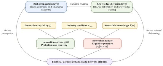
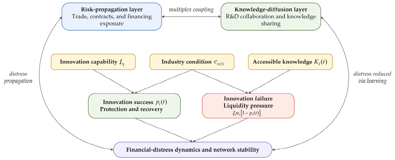
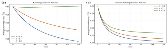
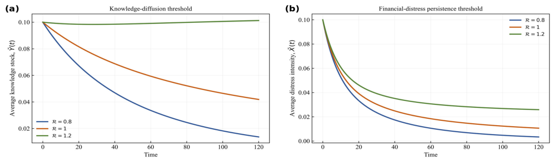
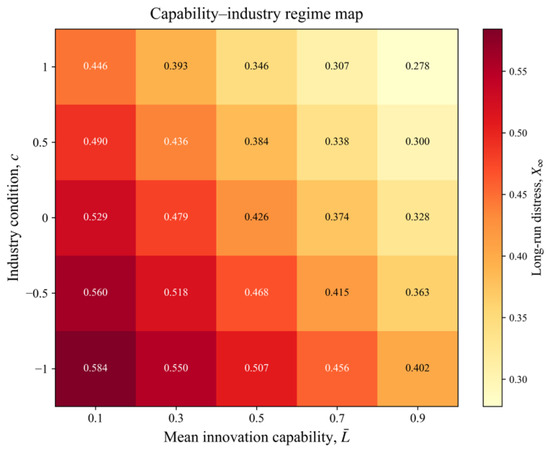
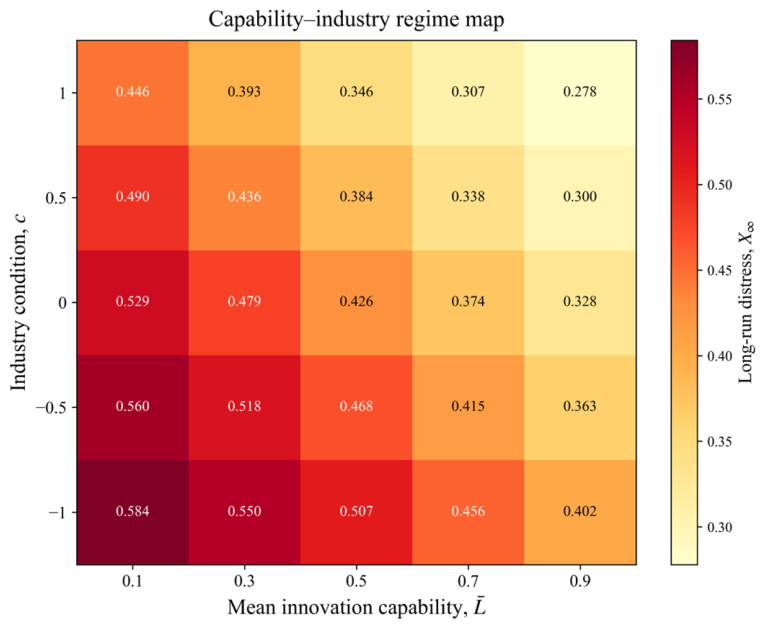
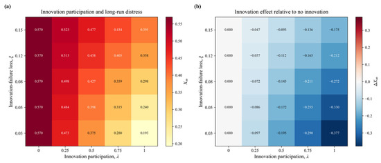
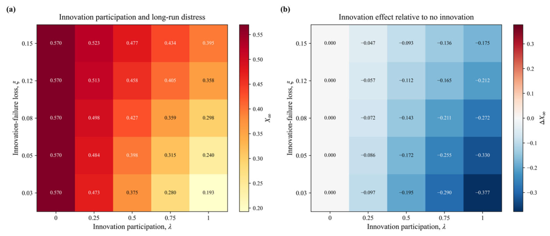
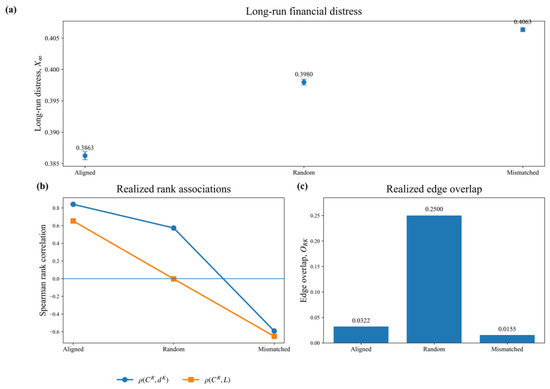
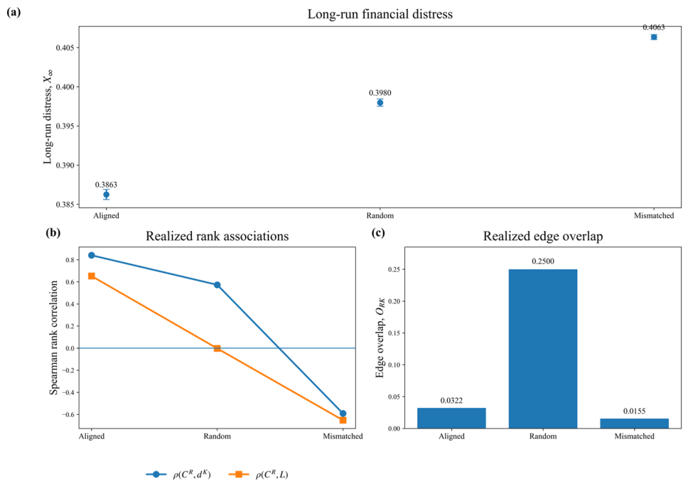
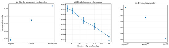
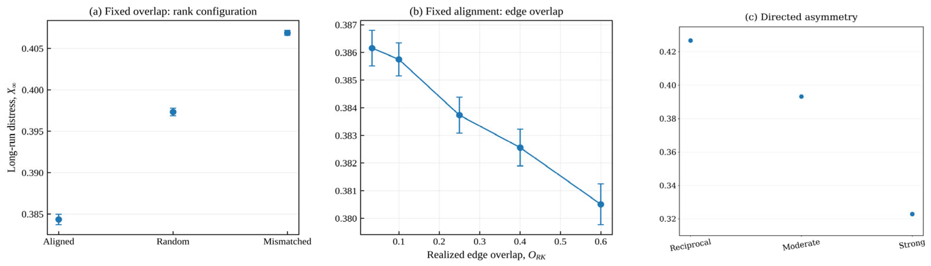
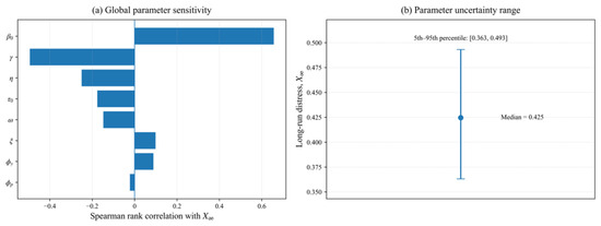
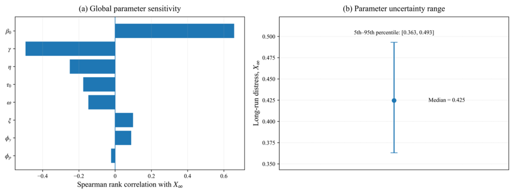

Disclaimer/Publisher’s Note: The statements, opinions and data contained in all publications are solely those of the individual author(s) and contributor(s) and not of MDPI and/or the editor(s). MDPI and/or the editor(s) disclaim responsibility for any injury to people or property resulting from any ideas, methods, instructions or products referred to in the content. |
© 2026 by the authors. Licensee MDPI, Basel, Switzerland. This article is an open access article distributed under the terms and conditions of the Creative Commons Attribution (CC BY) license.