Article

Transverse Bifurcations Occurring on Simple Robust Homoclinic Cycles

School of Mathematical Sciences, Beihang University, Beijing 100191, China
*
Author to whom correspondence should be addressed.
Mathematics 2026, 14(16), 3012; https://doi.org/10.3390/math14163012
Submission received: 20 July 2026 / Revised: 16 August 2026 / Accepted: 18 August 2026 / Published: 20 August 2026

Abstract

This paper studies codimension-one transverse bifurcations of several classes of simple robust homoclinic cycles in group-symmetric systems on R 5 . The analysis follows a complete classification induced by the representation of the symmetric group. Sufficient conditions are established under which new homoclinic cycles or heteroclinic connections bifurcate from the original cycle. An asymptotic expansion of the Poincaré map is derived, yielding explicit criteria for the bifurcation of periodic orbits from such homoclinic cycles and for determining their stability.

1. Introduction

Homoclinic and heteroclinic cycles frequently emerge in dynamical systems with symmetries, particularly in those related to fluid dynamics [1] and population dynamics [2,3]. A heteroclinic cycle is an invariant closed curve formed by a finite number of equilibria and trajectories. Heteroclinic cycles are generally structurally unstable in general dynamical systems, but can persist in symmetric systems under symmetry-preserving perturbations provided that each trajectory is robustly contained in a flow-invariant subspace forced by the symmetry. If all equilibria in the cycle belong to a group orbit associated with a symmetry, the resulting heteroclinic cycle is called a homoclinic cycle.
The first robust homoclinic cycle was introduced by Guckenheimer and Holmes [4] in the context of a three-dimensional system studied by [1], which involves three equilibria. Since the work of [4], simple robust homoclinic cycles in R k with k 5 have been extensively studied. The classification and stability analysis of homoclinic cycles in R 3 are relatively straightforward, as these cycles are structurally elementary. Field and Swift [5] first analyzed the case in R 4 , generalizing the earlier work of Guckenheimer [4]. Chossat et al. [6] classified simple homoclinic cycles in R 4 into three types. Subsequently, Sottocornola [7] further proposed a symmetry-based classification, which identifies groups that admit robust cycles.
However, a complete theory for the stability and bifurcations of heteroclinic and homoclinic cycles remains unavailable. Krupa and Melbourne [8,9,10] systematically studied simple robust heteroclinic cycles in R 4 , establishing necessary and sufficient conditions for asymptotic stability. This stability is associated with the eigenvalues of the linearization of the vector field at equilibria within the cycles, where the eigenvalues corresponding to eigenvectors outside the flow-invariant subspaces are called transverse.
The stability and bifurcation of simple robust heteroclinic cycles have been extensively studied [11,12,13,14,15]. The bifurcations of three-dimensional cycles have also been discussed, for instance in [16]. Chossat et al. [6], motivated by instabilities of magnetic field considered in [17], investigated the transverse bifurcation exhibited by simple homoclinic cycles in R 4 , which occurs when the real part of a transverse eigenvalue crosses zero. Driesse and Homburg [18] analyzed the resonance bifurcation for different types of homoclinic cycles, which occurs as the real parts of these eigenvalues satisfy a specific algebraic condition.
Sottocornola [19] investigated simple homoclinic cycles with two-dimensional invariant subspaces in R 5 and, within the special orthogonal group SO ( 5 ) , classified the minimal admissible groups—the simplest groups allowing such cycles. Podvigina [20] extended this work by systematically enumerating all possible classes of simple homoclinic cycles and their symmetry group in R 5 . Furthermore, she introduced a general classification in R n based on the representation of the isotropy subgroup of the fixed-point subspace on its orthogonal complement, establishing for each class the conditions for asymptotic and fragmentary asymptotic stability. Unlike their lower-dimensional analogs, the bifurcations of simple homoclinic cycles in dimensions five and above remain largely unexplored. As far as we are aware, the only existing results concern cycles with specific symmetry groups [21,22].
The aim of this paper is to take a step towards filling this gap by investigating codimension-one transverse bifurcations of simple robust homoclinic cycles in R 5 , triggered by a transverse eigenvalue crossing zero. Our analysis follows the Poincaré-map program initiated by Chossat et al. [6] for R 4 , together with the classification of Podvigina [20,23]: after reducing the local dynamics near each equilibrium to normal form, we derive the asymptotic expansion of the first-return map along the heteroclinic connections, from which we obtain explicit bifurcation criteria. It is instructive to contrast this mechanism with alternative techniques developed outside the equivariant framework.
Geometric Singular Perturbation Theory (GSPT) is concerned with multiple-time-scale (fast−slow) dynamical systems that depend on a small parameter. Its theoretical basis is Fenichel theory, and relaxation oscillations (periodic solution) arise from the analysis of the fast and slow subsystems [24,25]. In most situations where normal hyperbolicity holds, the approximation of high-dimensional systems by low-dimensional models is mathematically rigorous and reliable, providing profound insights across diverse fields ranging from neuroscience to chemical reactions. When the transverse dynamics is much slower than that within the cycle, the Poincaré map expansion yields an effective slow dynamics that GSPT can interpret geometrically [26]. Melnikov-type and Lin’s methods instead treat structurally unstable connections via splitting integrals or jump conditions [27,28]; here the connections persist by symmetry-forced invariant subspaces [4]. In hyperbolic reaction–transport models, traveling waves are obtained as heteroclinic orbits of the traveling-wave ODE [29,30,31]; our framework instead treats the equivariant ODE directly and yields criteria that hold uniformly for entire classes of cycles.
In particular, we focus on the loss of asymptotic stability in the associated homoclinic network. For several classes, we establish the existence of a periodic orbit bifurcating from the cycle and provide sufficient conditions for its stability; for the other classes, we prove the emergence of either new homoclinic cycles or heteroclinic trajectories joining equilibria within the original network. Theorems 1, 2, and 4 can be regarded as direct extensions of the results of [6] from R 4 to R 5 , since the cycles involved possess symmetry structures and expressions of the Poincaré map analogous to those of the corresponding cycles in [6]. The bifurcations described in Theorems 3 and 5, however, are specific to R 5 ; for these classes different arguments are required.
The paper is organized as follows. Section 2 introduces the key definitions and reviews existing classifications of simple homoclinic cycles in R 5 . Section 3 derives the associated Poincaré map. Section 4 and Section 5 are devoted to the transverse bifurcation analysis of type Z and type A cycles respectively. Section 6 investigates bifurcations of the remaining types of cycles. Finally, Section 7 provides concluding remarks.

2. Preliminaries

2.1. Robust Heteroclinic Cycle

We start with some simple and essential definitions [32]. Let
x ˙ = d x d t = f ( x , λ ) , x R n , λ R ,
be a system of ordinary differential equations, where λ is a real parameter and f : R n × R R n is smooth. Let γ be an invertible n × n matrix. Then γ is called a symmetry of (1) (or f) if
f ( γ x , λ ) = γ f ( x , λ )
for all ( x , λ ) R n × R . From (2) it follows directly that if ϕ ( t ) solves (1), then so does γ ϕ ( t ) . In the particular case of an equilibrium ϕ ( t ) x 0 , this means that γ x 0 is also an equilibrium. If γ x 0 x 0 , this yields a new equilibrium; if γ x 0 = x 0 , then γ is said to be a symmetry of the equilibrium x 0 . When enumerating all equilibria of (1), one need only consider orbits of the symmetry group, since all other equilibria are obtained by the action of the symmetries of f.
Equation (2) also implies that symmetries map T periodic solutions to T periodic solutions: if ϕ ( t ) is a T periodic solution of (1), then γ ϕ ( t ) is again T periodic. In the periodic setting, however, it is natural to broaden the notion of a symmetry of a solution. By uniqueness for the initial value problem, the trajectories of ϕ ( t ) and γ ϕ ( t ) are either disjoint—giving a distinct periodic solution—or identical. In the latter case, the two solutions differ only by a phase shift, that is,
ϕ ( t ) = γ ϕ ( t t 0 )
for some t 0 . We then call the pair ( γ , t 0 ) a symmetry of the periodic solution ϕ ( t ) . Hence, symmetries of periodic solutions possess both a spatial part γ and a temporal part t 0
Let O ( n ) denote the n dimensional orthogonal group, consisting of all n × n matrices A over R satisfying
A A T = I n ,
where I n is the n × n identity matrix and A T is the transpose of A.
From now on, we assume Γ is a nontrivial finite group acting linearly on R n . Without loss of generality, we assume Γ O ( n ) is a subgroup of orthogonal group O ( n ) [16,19].
We shall henceforth take system (1) to be Γ -equivariant, i.e., (2) is satisfied for all γ Γ . In other words, each member of Γ is a symmetry of (1).
Let ξ j ( j = 1 , 2 , , m ) be hyperbolic equilibria of the system (1) with their stable manifolds and unstable manifolds denoted by W s ( ξ j ) and W u ( ξ j ) , respectively. A solution trajectory ϕ ( t ) of the system (1) is called a heteroclinic trajectory from an equilibrium ξ to another ξ if it is backward asymptotic to ξ , and forward to ξ , i.e.,
lim t ϕ ( t ) = ξ and lim t + ϕ ( t ) = ξ .
For each j = 1 , 2 , , m , we denote by ϕ j = ϕ j ( t ) a heteroclinic trajectory from ξ j to ξ j + 1 .
Before proceeding, we recall a few definitions and lemmas necessary for our discussion.
Definition 1.
The collection of equilibria and trajectories { ξ j , ϕ j ( t ) , j = 1 , 2 , , m } is called a heteroclinic cycle if ξ m + 1 = ξ 1 .
Definition 2
([20]). A heteroclinic cycle is termed a homoclinic cycle, if there exists an element γ Γ such that
γ ξ j = ξ j + 1 , j = 1 , 2 , , m .
Such symmetry γ is called a twist.
We recall that for a subgroup Σ Γ , its fixed-point subspace is given by
Fix ( Σ ) = { x R n σ x = x , σ Σ } .
It follows from the equivariance of the system that every fixed-point subspace is flow-invariant.
A subgroup Σ of Γ is said to be the isotropy subgroup of a subset S R n if
Σ = { γ Γ : γ x = x , for all x S } .
By the Proposition 2.5 of [8], a heteroclinic cycle is structurally stable (under Γ equivariant perturbation) if, for each j { 1 , 2 , , m } , there exists a subgroup Σ j Γ whose fixed-point subspace is P j : = Fix ( Σ j ) , with Σ j being the isotropy subgroup of P j , such that
  • ξ j + 1 is a sink in P j ;
  • ϕ j P j .
Structurally stable heteroclinic (or homoclinic) cycles are also known as robust heteroclinic (or homoclinic) cycles.
Let L j : = P j 1 P j for j = 1 , 2 , , m , with the convention that P 0 = P m . The isotropy subgroup of L j is denoted by Ω j ; note that ξ j L j .
Definition 3
([23]). A robust heteroclinic cycle in R n { 0 } is called simple, if
dim ( P j 1 L j ) = 1 , j = 1 , 2 , , m ,
and all eigenvalues of the linearization d f ( ξ j ) are distinct.
The following lemma shows that for a simple robust heteroclinic cycle, the fixed-point subspaces P j all have the same dimension.
Lemma 1
([20]). If a robust heteroclinic cycle is simple, then dim P j = dim P j + 1 for all j = 1 , 2 , , m 1 .
Definition 4
([23]). A simple robust heteroclinic cycle is said to be of type Z if, for every j, the isotropy subgroup Σ j of P j decomposes P j into one-dimensional isotypic components.
Definition 5
([20]). A simple robust heteroclinic cycle is said to be of type A if, for every j, the isotypic decomposition of P j under the action of Σ j contains exactly one isotypic component.
Definition 6
([20]). A homoclinic network is a connected component of the Γ orbit of a homoclinic cycle.
Following the classification established in [8,20], for a structurally stable heteroclinic cycle, the eigenvalues of d f ( ξ j ) are divided into four types according to the location of their corresponding eigenspaces:
  • Radial eigenvalues: Those whose eigenspace is contained in L j .
  • Contracting eigenvalues: Those whose eigenspace is contained in P j 1 L j .
  • Expanding eigenvalues: Those whose eigenspace is contained in P j L j .
  • Transverse eigenvalues: Those whose eigenspace is orthogonal to all the subspaces above.
To simplify notation, we will often omit the subscripts from P j , ξ j , and ϕ j in subsequent discussion when no ambiguity arises.
Assume that the eigenvalues of d f ( ξ j ) are of the following types:
  • radial eigenvalues r l ( 1 l n r ) ;
  • a unique contracting eigenvalue c < 0 ;
  • a unique expanding eigenvalue e > 0 ;
  • transverse eigenvalues t l ( 1 l n t ) .
In what follows, the term homoclinic cycle will always mean a simple robust homoclinic cycle.
Definition 7.
Let λ 1 , , λ n be the eigenvalues of d f ( ξ ) . They are said to satisfy the nonresonance condition up to order N if
λ i j = 1 n a j λ j , i = 1 , 2 , , n
holds for all nonnegative integers a 1 , a 2 , , a n with 2 j = 1 n a j N .
In this paper, we consider only those homoclinic cycles for which the eigenvalues of the linearization d f ( ξ ) —apart from the eigenvalue corresponding to the bifurcation direction—have real parts that satisfy the nonresonance condition to all orders N N .

2.2. Stability of Homoclinic Cycles in R n

We write ϕ t ( x ) = ϕ ( t , x ) for the trajectory of system (1) starting from x, called the flow (or the flow map) generated by the vector field defined by system (1). For a compact invariant set X R n of system (1) and a number δ > 0 , we define its δ neighborhood as
N δ ( X ) = { x R n : d ( x , X ) < δ } ,
and its δ local basin of attraction as
B δ ( X ) = x R n : ϕ t ( x ) N δ ( X ) for t 0 , and lim t + d ( ϕ t ( x ) , X ) = 0 .
Definition 8.
A compact subset X R n that is positively invariant under the flow ϕ ( t , x ) is called stable if, for every δ > 0 , there exists δ 1 > 0 such that
ϕ ( t , N δ 1 ( X ) ) N δ ( X ) , t 0 .
X is called asymptotically stable if it is both stable and attracting; that is, if its basin of attraction
B ( X ) = { x R n : lim t + d ( ϕ t ( x ) , X ) = 0 }
is a neighborhood of X.
A homoclinic cycle itself cannot be asymptotically stable by definition since the unstable manifold of ξ i contains another trajectory that lies outside the homoclinic cycle. Following [12,23], we say a homoclinic cycle is asymptotically stable when the homoclinic network containing it is asymptotically stable.

2.3. Classification of Homoclinic Cycles in R n

Here we present the classification of homoclinic cycles in R n as given in [20].
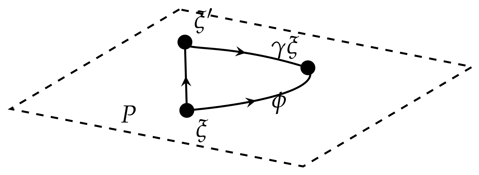
Let X R n be a homoclinic cycle of (1), ξ X an equilibrium, and P the invariant plane containing ξ and γ ξ . We define two bases for P as follows:
B 1 = { p k : 1 k K } ; B 2 = { q k : 1 k K } ,
where the p k are eigenvectors of d f ( ξ )   ( p 1 contracting); the q k are eigenvectors of d f ( γ ξ ) ( q 1 expanding), while the transverse eigenvectors satisfy q k = γ p k for 2 k K .
We assume that the isotypic decomposition of P under the action of Σ takes the form
P = V 1 V J .
Due to the invariance of both the isotypic components and the eigenspaces of d f ( ξ ) and d f ( γ ξ ) , each isotypic component V i ( i = 1 , 2 , , J ) is spanned by vectors belonging exclusively to either B 1 or B 2 .
Assume q 1 V 1 .We arrange the eigenvectors in B 2 so that the q k belonging to each V i appear with consecutive indices. Setting dim V i = l i and s i = k = 1 i l k for i = 1 , , J , this ordering yields
V 1 = span { q 1 , , q s 1 } V 2 = span { q s 1 + 1 , , q s 2 } V J = span { q s J 1 + 1 , , q s J } .
Likewise, each isotypic component V j is spanned by some eigenvectors p k whose indices range over k = i s j 1 + 1 , i s j 1 + 2 , , i s j 1 + s j . That is
V j = span p k B 1 : k { i s j 1 + 1 , i s j 1 + 2 , , i s j } ,
where the indices { i 1 , i 2 , , i s J } form a permutation of { 1 , 2 , , s J } .
Let m = dim P . The homoclinic cycle is labeled by a sequence of numbers, with square brackets grouping the subsequences that correspond to the individual isotypic components:
m [ i 1 , , i s 1 ] V 1 [ i s 1 + 1 , , i s 2 ] V 2 [ i s J 1 + 1 , , i s J ] V J .
For example, the homoclinic cycle X of class 3-[12][3] in R 5 refers to a configuration where dim P = 3 and P consists of two isotypic components. The associated subspaces are:
dim V 1 = 2 , V 1 = span { p 1 , p 2 } , q 1 V 1 ; dim V 2 = 1 , V 2 = span { p 3 } .
The following lemma implies that not every permutation inside the brackets can occur in a homoclinic cycle constructed this way.
Lemma 2
([20]). Let X be a simple robust homoclinic cycle of the Γ-equivariant system, and let
P = V 1 V J
be the isotypic decomposition under Σ Γ . Denote by V * the component containing p 1 . Following the ordering described above, take q 1 V 1 , Then the following properties hold:
(i) 
dim V 1 = dim V * .
(ii) 
γ p j V 1 for any p j V * .

2.4. Classification and Stability of Homoclinic Cycles in R 5

We review the complete classification of homoclinic cycles in R 5 and their class-wise stability conditions, following [20].
Let d denote the dimension of the fixed-point subspace P associated with a homoclinic cycle, where d can be 4, 3, or 2. The classification according to d is given as follows:
  • For d = 4 , there is exactly one class, denoted by 1-[1].
  • For d = 3 , there are three distinct classes: 2-[12], 2-[1][2], and 2-[2][1].
  • For d = 2 , there are seven classes: 3-[123], 3-[1][2][3], 3-[2][1][3], 3-[2][3][1], 3-[1][3][2], 3-[1][23], and 3-[12][3].
The 1-[1] class exhibits no transverse eigenvalues and thus offer no scope for transverse stability analysis. Accordingly, such cycles are excluded from the subsequent discussion.
We recall the notation for the eigenvalues of d f ( ξ ) : (i) radial eigenvalues r l for 1 l d 1 ( d = 2 or 3 ), (ii) a unique contracting eigenvalue c , (iii) a unique expanding eigenvalue e, (iv) transverse eigenvalues t l for 1 l 4 d .
Table 1, adapted from Table 4 of [20], presents asymptotic stability conditions for different classes of cycles.
Assuming all eigenvalues of d f ( ξ ) are real and distinct, each eigenspace is one-dimensional. Since d f ( ξ ) commutes with the symmetry group Σ , each eigenspace is Σ invariant. Thus, for any eigenvector v, any σ Σ must map v to a scalar multiple of itself. Given the multiplicative action of the group, this scalar is restricted to ± 1 . Therefore, the representation of Σ on each isotypic component is either the identity id or id . Moreover, there must exist some σ Σ that acts as 1 on the isotypic component containing the transverse eigenvalues. Otherwise, the entire group Σ would act trivially on that component, implying the corresponding directions are fully symmetric under Σ , which defines them as radial rather than transverse.

3. Poincaré Maps for Simple Homoclinic Cycles in R 5

We now turn to constructing the Poincaré maps for the homoclinic cycles of system (1) when n = 5 , assuming the eigenvalues of d f ( ξ ) are distinct. Let γ represent the twist associated with the homoclinic cycle.

3.1. The Case dim P = 2

Without loss of generality, we assume the transverse eigenvalue t 2 ( λ ) passes through zero transversely near λ = 0 ; that is t 2 ( 0 ) = 0 , t 2 ( 0 ) 0 . (If not, we simply relabel t 1 and t 2 ). Moreover, by rescaling the parameter we may take t 2 ( 0 ) > 0 and subsequently reparameterize so that t 2 ( λ ) λ .
Under the nonresonance conditions, it was shown by Takens [33] and Bonckaert [34] that for any positive integer k, for | λ | sufficiently small, the system (1) is locally C k -equivalent in a neighborhood of ξ to a system of the type:
u ˙ = r ( z 2 , λ ) u v ˙ = c ( z 2 , λ ) v w ˙ = e ( z 2 , λ ) w z 1 ˙ = t 1 ( z 2 , λ ) z 1 z 2 ˙ = Z 2 ( z 2 , λ ) ,
where r ( z 2 , λ ) , c ( z 2 , λ ) , e ( z 2 , λ ) , t 1 ( z 2 , λ ) , Z 2 ( z 2 , λ ) are all C k functions of z 2 and λ . By symmetry, Z 2 admits the local expansion near z 2 = 0 :
Z 2 ( z 2 , λ ) = t 2 ( λ ) z 2 + h ( z 2 , λ ) = λ z 2 + h ( z 2 , λ ) , h ( z 2 , λ ) = O ( | z 2 | 3 ) .
We further assume the generic condition 3 h z 2 3 ( 0 , 0 ) 0 .
For a sufficiently small δ > 0 , we rescale the variables via
u δ u ; v δ v ; w δ w ; z 1 δ z 1 ; z 2 δ z 2 .
Let ( u 0 , v 0 , 0 , 0 , 0 ) γ 1 P be the intersection point of the heteroclinic trajectory with the sphere u 2 + v 2 = 1 . Assuming v 0 > 0 (which can be achieved by symmetry), we further renormalize the v coordinate by v v 0 v . We then define the local cross-sections
H i n = { ( u , 1 , w , z 1 , z 2 ) : | u | , | w | , | z 1 | , | z 2 |   < 1 } , H o u t = { ( u , v , 1 , z 1 , z 2 ) : | u | , | v | , | z 1 | , | z 2 |   < 1 } ,
which are evidently traversed by the homoclinic cycle.
We define the first hit map φ : H i n H o u t for system (1) in a neighborhood of ξ . For a point ( u , 1 , w , z 1 , z 2 ) H i n with w > 0 , and sufficiently small coordinates, the forward trajectory of system (6) starting from it yields a first intersection point near ξ with H o u t , which is taken as φ ( u , w , z 1 , z 2 ) . This map is well defined for points sufficiently close to the homoclinic cycle.
Lemma 3.
Suppose w > 0 , then the first hit map φ takes the form
φ ( u , w , z 1 , z 2 ) = u w r 0 e 0 ( 1 + O ( z 2 ) ) w c 0 e 0 ( 1 + O ( z 2 ) ) z 1 w t 10 e 0 ( 1 + O ( z 2 ) ) z 2 w λ e 0 ( 1 + O ( z 2 ) ) T ,
where c ( 0 , λ ) = c 0 , e ( 0 , λ ) = e 0 , r ( 0 , λ ) = r 0 , t 1 ( 0 , λ ) = t 10 .
Proof. 
To avoid confusion, we denote the initial coordinates by ( u 0 , 1 , w 0 , x 0 , z 0 ) H i n . Introduce the time reparametrization e ( z 2 , λ ) d t = d τ , which yields d w d τ = w and hitting time T = ln w 0 ( w 0 > 0 ) . Let z 2 ( τ , z 0 ; λ ) be the solution of
d z 2 d τ = λ z 2 + h ( z 2 , λ ) e ( z 2 , λ ) = λ e 0 z 2 + h * ( z 2 , λ ) .
where h * ( z 2 , λ ) = h ( z 2 , λ ) e ( z 2 , λ ) + λ e ( z 2 , λ ) λ e 0 z 2 , with a small initial condition z 2 ( 0 ) = z 0 . Since h * ( z 2 , λ ) inherits the invariance h * ( z 2 , λ ) = h * ( z 2 , λ ) , its Taylor expansion about z 2 = 0 contains only odd powers of z 2 . So, z 2 0 is a solution of (7).
The solution of (7) can be written formally as
z 2 ( τ , z 0 ; λ ) = e λ τ / e 0 z 0 + 0 τ e λ s / e 0 h * ( z 2 , λ ) d s .
Setting τ = T = ln w 0 , then gives
z 2 ( T , z 0 ; λ ) = w 0 λ / e 0 z 0 + 0 ln w 0 e λ s / e 0 h * ( z 2 , λ ) d s .
To evaluate the integral 0 ln w 0 e λ s / e 0 h * ( z 2 , λ ) d s , we first need an estimate for z 2 ( T , z 0 ; λ ) .
We begin with the case z 0 > 0 ; the case z 0 < 0 follows similarly.
Choose a sufficiently small constant ε > 0 and restrict the parameter to the regime | λ | < 1 2   min { e 0 , 1 } ϵ . By h * ( z 2 , λ ) = O ( | z 2 | 3 ) , the inequality
λ e 0 z 2 + h * ( z 2 , λ ) ϵ z 2
holds for all 0 z 2 < ϵ . To obtain an estimate for z 2 , we first consider the auxiliary equation
z 2 ˙ = ϵ z 2 .
By the comparison lemma and uniqueness of Equation (7), we have
0 z 2 ( τ , z 0 ; λ ) z 0 e ϵ τ , 0 τ a , 0 z 2 < ϵ
for some a. Choosing sufficiently small initial conditions satisfying z 0 < w 0 < 1 4 ϵ 2 , we have
z 0 e ϵ T = z 0 w 0 ϵ < z 0 1 ϵ < 1 2 ϵ 2 2 ϵ < ϵ .
Since h * ( z 2 , λ ) is at least of third order in z 2 , there exist a constant C such that
0 T e λ s e 0 h * ( z 2 , λ ) d s < C T max 0 t T | z 2 | 3 < C | ln z 0 | z 0 3 3 ϵ < C z 0 2 .
Consequently, z 2 ( T , z 0 ; λ ) = z 0 w 0 λ / e 0 ( 1 + O ( z 0 ) ) .
The equation for v in the τ variable reads
d v d τ = c ( z 2 ( τ , z 0 ; λ ) , λ ) e ( z 2 ( τ , z 0 ; λ ) , λ ) v = c 0 e 0 + c 1 ( z 2 ( τ , z 0 ; λ ) , λ ) v ,
where c 1 ( z 2 , λ ) = O ( z 2 ) . The solution of (11) is
v ( τ ) = e τ c 0 e 0 + 0 τ c 1 ( z 2 ( s , z 0 ; λ ) , λ ) d s .
Evaluating at the hitting time T = ln w 0 yields
v ( T ) = w 0 c 0 e 0 e 0 ln w 0 c 1 ( z 2 ( s , z 0 ; λ ) , λ ) d s .
Applying 0 z 2 ( τ , z 0 ; λ ) z 0 e ϵ τ and c 1 ( 0 , λ ) = 0 , we conclude that
v ( T ) = w 0 c 0 e 0 ( 1 + O ( z 0 ) ) .
The analysis for the u-component and z 1 -component follows similarly. The proof is finished by substituting initial condition back.    ☐
The connecting diffeomorphism ψ : H o u t γ H i n is induced by the trajectories of system (1) near the heteroclinic trajectory ϕ from ξ to γ ξ . The map γ 1 ψ ( u , v , z 1 , z 2 ) admits a linear approximation of the form
γ 1 ψ ( u , v , z 1 , z 2 ) = M ( u , v , z 1 , z 2 ) T + O ( u , v , z 1 , z 2 ) 2 ,
where M is the 4 × 4 matrix given by the linearization of the connecting diffeomorphism γ 1 ψ at ( 0 , 1 , 0 , 0 ) :
M = a 11 a 12 a 13 a 14 0 a 22 a 23 a 24 0 a 32 a 33 a 34 0 a 42 a 43 a 44 .
The zeros in the first column follow from the invariance of P: for any ( u , 0 , 0 , 0 ) H o u t , we have ψ ( u , 0 , 0 , 0 ) P , so the w , z 1 , z 2 -components of γ 1 ψ ( u , 0 , 0 , 0 ) vanish identically. The diagonal entries a 11 , a 22 , a 33 , a 44 are generically nonzero. In contrast, the off-diagonal entries may vanish for certain symmetry group structures, and the generic nonvanishing conditions required for our results are imposed on these entries only when they are needed in the subsequent theorems (see Section 5 and Section 6).
The Poincaré map g = γ 1 ψ φ can be presented by
g ( u , w , z 1 , z 2 ) = η ( u , w , z 1 , z 2 , λ ) a 22 w c 0 e 0 + a 23 z 1 w t 10 e 0 + a 24 z 2 w λ e 0 + ω 1 ( u , w , z 1 , z 2 ) a 32 w c 0 e 0 + a 33 z 1 w t 10 e 0 + a 34 z 2 w λ e 0 + ω 2 ( u , w , z 1 , z 2 ) a 42 w c 0 e 0 + a 43 z 1 w t 10 e 0 + a 44 z 2 w λ e 0 + ω 3 ( u , w , z 1 , z 2 ) T
where η is smooth in the variables u , w , z 1 , z 2 and the parameter λ with the asymptotic form:
η = a 11 u w r 0 e 0 ( 1 + O ( z 2 ) ) + a 12 w c 0 e 0 ( 1 + O ( z 2 ) ) + a 13 z 1 w t 10 e 0 ( 1 + O ( z 2 ) ) + a 14 z 2 w λ e 0 ( 1 + O ( z 2 ) ) + O ( ( u w r 0 e 0 , w c 0 e 0 , z 1 w t 10 e 0 , z 2 w λ e 0 ) k ) ,
and the functions ω i ( w , z 1 , z 2 ) ( i = 1 , 2 , 3 ) have the asymptotic forms:
ω 1 = w c 0 e 0 O ( z 2 ) + z 1 w t 10 e 0 O ( z 2 ) + z 2 w λ e 0 O ( z 2 ) + O w c 0 e 0 , z 1 w t 10 e 0 , z 2 w λ e 0 u w r 0 e 0 , w c 0 e 0 , z 1 w t 10 e 0 , z 2 w λ e 0 k 1 , ω 2 = w c 0 e 0 O ( z 2 ) + z 1 w t 10 e 0 O ( z 2 ) + z 2 w λ e 0 O ( z 2 ) + O w c 0 e 0 , z 1 w t 10 e 0 , z 2 w λ e 0 u w r 0 e 0 , w c 0 e 0 , z 1 w t 10 e 0 , z 2 w λ e 0 k 1 , ω 3 = w c 0 e 0 O ( z 2 ) + z 1 w t 10 e 0 O ( z 2 ) + z 2 w λ e 0 O ( z 2 ) + O w c 0 e 0 , z 1 w t 10 e 0 , z 2 w λ e 0 u w r 0 e 0 , w c 0 e 0 , z 1 w t 10 e 0 , z 2 w λ e 0 k 1 .
as ( w , z 1 , z 2 , λ ) ( 0 , 0 , 0 , 0 ) , where k 2 .

3.2. The Case dim P = 3

Under the nonresonance conditions, for any positive integer k, the systems (1) are locally C k -equivalent in some neighborhood of ξ to a system of the form:
u ˙ 1 = r 1 ( z , λ ) u 1 u ˙ 2 = r 2 ( z , λ ) u 2 v ˙ = c ( z , λ ) v w ˙ = e ( z , λ ) w z ˙ = Z ( z , λ ) ,
where Z ( z , λ ) is a C k function of z and λ . As in the case dim P = 2 , we set the transverse eigenvalue t ( λ ) λ . Expanding Z about z = 0 yields
Z ( z , λ ) = t ( λ ) z + h ( z , λ ) = λ z + h ( z , λ ) , h ( z , λ ) = O ( | z | 3 ) .
We also make the generic assumption that the cubic term is nondegenerate, i.e, 3 z 3 ( 0 , 0 ) 0 .
Then we rescale the coordinates ( u 1 , u 2 , v , w , z ) and choose the cross-sections
H i n = { ( u , 1 , w , z ) : | u | , | w | , | z | < 1 } , H o u t = { ( u , v , 1 , z ) : | u | , | v | , | z | < 1 } ,
where u = ( u 1 , u 2 ) . We define, as before, the first−hit map φ : H i n H o u t system (1) by the forward trajectories of system (12) near ξ . Denote c ( 0 , λ ) = c 0 , e ( 0 , λ ) = e 0 , r 1 ( 0 , λ ) = r 10 , r 2 ( 0 , λ ) = r 20 .
Lemma 4.
The first hit map φ takes the form
φ ( u 1 , u 2 , w , z ) = u 1 w r 10 e 0 ( 1 + O ( z ) ) u 2 w r 20 e 0 ( 1 + O ( z ) ) w c 0 e 0 ( 1 + O ( z ) ) z w λ e 0 ( 1 + O ( z ) ) T .
The proof is analogous to that of Lemma 3 and is therefore omitted.
Then we consider a connecting diffeomorphism ψ : H o u t γ H i n .
The map γ 1 ψ ( u 1 , u 2 , v , z ) admits a linear approximation of the form
γ 1 ψ ( u 1 , u 2 , v , z ) = M ( u 1 , u 2 , v , z ) T + O ( | ( u 1 , u 2 , v , z ) | 2 ) ,
where
M = a 11 a 12 a 13 a 14 a 21 a 22 a 23 a 24 0 0 a 33 a 34 0 0 a 43 a 44 .
The 2 × 2 zero block in the lower-left corner also follows from the invariance of P: for any ( u 1 , u 2 , 0 , 0 ) H o u t , we have ψ ( u 1 , u 2 , 0 , 0 ) P , so the last two components of γ 1 ψ ( u 1 , u 2 , 0 , 0 ) vanish identically. The diagonal entries a 11 , a 22 , a 33 , a 44 are generically nonzero while the generic nonvanishing conditions on the off-diagonal entries specially required for our results are imposed on these entries in the subsequent theorems (see Section 5).
So the Poincaré map g = γ 1 ψ φ can be presented by
g ( u 1 , u 2 , w , z ) = η 1 ( u 1 , u 2 , w , z , λ ) η 2 ( u 1 , u 2 , w , z , λ ) a 33 w c 0 e 0 + a 34 z w λ e 0 + ω 4 ( u 1 , u 2 , w , z ) a 43 w c 0 e 0 + a 44 z w λ e 0 + ω 5 ( u 1 , u 2 , w , z ) T ,
where η 1 and η 2 are smooth functions of u 1 , u 2 , w , z and parameter λ with the asymptotic forms:
η 1 = a 11 u 1 w r 10 e 0 ( 1 + O ( z ) ) + a 12 u 2 w r 20 e 0 ( 1 + O ( z ) ) + a 13 w c 0 e 0 ( 1 + O ( z ) ) + a 14 z w λ e 0 ( 1 + O ( z ) ) + O ( ( u 1 w r 10 e 0 , u 2 w r 20 e 0 , w c 0 e 0 , z w λ e 0 ) k ) , η 2 = a 21 u 1 w r 10 e 0 ( 1 + O ( z ) ) + a 22 u 2 w r 20 e 0 ( 1 + O ( z ) ) + a 23 w c 0 e 0 ( 1 + O ( z ) ) + a 24 z w λ e 0 ( 1 + O ( z ) ) + O ( ( u 1 w r 10 e 0 , u 2 w r 20 e 0 , w c 0 e 0 , z w λ e 0 ) k ) ,
and the functions ω 4 and ω 5 have the asymptotic forms:
ω 4 ( u 1 , u 2 , w , z ) = w c 0 e 0 O ( z ) + z w λ e 0 O ( z ) + O w c 0 e 0 , z w λ e 0 u 1 w r 10 e 0 , u 2 w r 20 e 0 , w c 0 e 0 , z w λ e 0 k 1 , ω 5 ( u 1 , u 2 , w , z ) = w c 0 e 0 O ( z ) + z w λ e 0 O ( z ) + O w c 0 e 0 , z w λ e 0 u 1 w r 10 e 0 , u 2 w r 20 e 0 , w c 0 e 0 , z w λ e 0 k 1 .
as w 0 , z 0 , λ 0 , where k 2 .

4. Transverse Bifurcation of Type Z

This section is devoted to the study of transverse bifurcations in type Z homoclinic cycles.
The classification of type-Z homoclinic cycles in R 5 is as follows:
  • For dim P = 3 : 2-[1][2], 2-[2][1].
  • For dim P = 2 : 3-[1][2][3], 3-[1][3][2], 3-[2][1][3], 3-[2][3][1].
For a homoclinic cycle of type Z, the isotypic components of P are eigenspaces of d f ( ξ ) , a consequence of their flow invariance. Furthermore, the direct product of any such component with P itself forms a subspace that is invariant under both the symmetry and the flow.
The following lemma establishes the existence of these invariant subspaces.
Lemma 5
([23]). Let a group Λ act on a linear space V. Consider the isotypic decomposition of the linear space under the action of Λ:
V = W 0 W 1 W K .
Suppose:
  • the action of Λ on W 0 is trivial;
  • any σ Λ acts on a W k , 1 k K , either as id or as -id.
Then for any collection of indices 1 i 1 , , i l K there exists a subgroup G i 1 , , i l Λ such that the subspace
V i 1 , , i l = W 0 W i 1 W i l
is a fixed-point subspace of the group G i 1 , , i l .
For cycles with dim P = 3 , d f ( ξ ) has a single transverse eigenvalue (with a one-dimensional eigenspace). For cycles with dim P = 2 , there are two transverse eigenvalues, thus giving rise to two distinct cases in which a transverse bifurcation can occur.
Therefore, before proceeding, we must assign labels to the isotypic components. For a given subspace P, we order the eigenvectors of d f ( ξ ) in P according to the classification given in the previous section, denoting them by { p 1 , p 2 } or { p 1 , p 2 , p 3 } . The isotypic components of P are then labeled as follows: the component containing the contracting eigenvector p 1 of d f ( ξ ) is designated as the first component U 1 ; the component containing p 2 is designated as the second component U 2 ; and, when present, the component containing p 3 is designated as the third component U 3 . The action of the twist γ on these isotypic components for all types is provided in Table 2:

4.1. The Case dimP = 3

When the parameter λ crosses zero, Equation (12) undergoes a pitchfork bifurcation near the equilibrium ξ , resulting in two new equilibria ξ and ξ . This bifurcation takes place within the second component U 2 of the local system (12), and hence ξ also lies in U 2 .
By Lemma 5, the subspaces Q = P U 2 and Q = P U 1 are invariant. In type 2-[1][2] cycles, P divides Q into two connected components. Since there exists an element σ Σ which acts as 1 on U 2 , we may assume (after replacing γ by σ γ if necessary) that γ preserves these components. For type 2-[2][1] cycles, P and γ P together divide Q into four connected components. In this case, we can also choose γ so that ξ and γ 2 ξ lie in the same component of Q.
The following theorem states that, alongside these pitchfork bifurcations, the homoclinic cycle, denoted by X, also undergoes a transverse bifurcation. This bifurcation produces new homoclinic cycles and is itself called a pitchfork bifurcation in [6]. We will analyze this bifurcation for the local system (12) (i.e., system (1)) under the following nondegeneracy condition:
r 1 ( 0 , 0 ) > 0 , r 2 ( 0 , 0 ) > 0 , c ( 0 , 0 ) > e ( 0 , 0 ) > 0 , t ( 0 ) = 0 , t ( 0 ) > 0 , h z z z ( 0 , 0 ) < 0
where h ( z , λ ) is defined by system (12).
Theorem 1.
If the nondegeneracy conditions (13) hold, and the real parts of all eigenvalues at ξ (except t ( λ ) ) satisfy a nonresonance condition up to a sufficiently high order N, then, for sufficiently small λ > 0 , new asymptotically stable homoclinic cycles bifurcate from X. Among them is a cycle X containing ξ such that:
(a) 
for type 2-[1][2], X includes the heteroclinic trajectory from ξ to γ ξ ;
(b) 
for type 2-[2][1], X includes the heteroclinic trajectory from ξ to γ 2 ξ .
Proof. 
For type 2-[1][2], γ preserves U 2 , and thus the pitchfork bifurcation at λ = 0 occurs in U 2 , producing four equilibria ξ , ξ , γ ξ , and γ ξ in Q when λ > 0 .
It suffices to search for the homoclinic cycles X containing ξ , since the group orbit of X consists of homoclinic cycles with identical stability properties.
The point ξ lies in the invariant subspace Q γ 1 Q . Its linearization d f ( ξ ) admits three negative eigenvalues: one close to r 1 , one close to r 2 , and one near 0. Furthermore, there exists a contracting eigenvalue close to c in γ 1 Q and an expanding eigenvalue close to e in Q. By the invariance of Q, the one-dimensional unstable manifold of ξ is contained in Q, which makes ξ a saddle inside Q. Under the action of γ , the expanding eigenvector of d f ( ξ ) is mapped into U 1 outside Q, so that γ ξ becomes a sink within Q.
We select a neighborhood B ( γ ξ , δ 1 ) in Q that contains both γ ξ and γ ξ for sufficiently small λ . Since the heteroclinic trajectories ϕ between ξ and γ ξ intersects B ( γ ξ , δ 1 ) , by continuity the unstable manifold of ξ also meets this neighborhood. Consider now trajectories starting in B ( γ ξ , δ 1 ) . These remain inside B ( γ ξ , δ 1 ) for all time and are attracted to one of the equilibria γ ξ , γ ξ , or γ ξ . Consequently, the unstable manifold of ξ is likewise attracted to one of these three equilibria.
Note that the stable manifold of γ ξ lies in P, and P divides Q into two flow-invariant components: one contains γ ξ and ξ , while the other contains γ ξ and ξ . The unstable manifold of ξ must therefore be attracted to γ ξ , which implies the existence of a new homoclinic cycle X formed by { γ j ξ j j = 1 , 2 , } together with their connecting trajectories. By definition, X is also a simple robust homoclinic cycle having Q as its invariant subspace. Applying the stability criterion for simple homoclinic cycles given in Table 1, we readily conclude that X is asymptotically stable.
For type 2-[2][1], we have γ U 1 = U 2 and γ U 2 = U 1 . Consequently, ξ undergoes a pitchfork bifurcation in Q, while γ ξ undergoes a pitchfork bifurcation in Q and γ 2 ξ again bifurcates in Q. For λ > 0 , the equilibria ξ , ξ , ξ , γ 2 ξ , γ 2 ξ , and γ 2 ξ lie in Q, whereas γ ξ and γ ξ lie in Q .
The eigenvalue structure of d f ( ξ ) is similar to that of type 2-[1][2]. Within the invariant subspace P γ 1 P , there are two negative eigenvalues: one close to r 1 and one close to r 2 . An additional eigenvalue close to 0 (yet negative) lies in U 2 , a contracting eigenvalue close to c lies in U 1 and an expanding eigenvalue close to e lies in P. The one-dimensional unstable manifold of ξ is contained in Q.
Under the action of γ , the expanding eigenvector of d f ( ξ ) is mapped to U 2 , implying that γ ξ is a saddle with a one-dimensional unstable manifold in Q. Moreover, γ 2 ξ is a saddle in Q, while γ 2 ξ is a sink in Q.
As before, we focus on trajectories emanating from ξ . We choose two small neighborhoods in Q: B ( γ 2 ξ , δ 2 ) , which contains the equilibria γ 2 ξ , γ 2 ξ , and γ 2 ξ for sufficiently small λ > 0 , and B ( γ ξ , δ 1 ) . Since γ ξ is a saddle in Q, trajectories starting in B ( γ ξ , δ 1 ) eventually leave the neighborhood, while those beginning in B ( γ 2 ξ , δ 2 ) converge to one of γ 2 ξ , γ 2 ξ , or γ 2 ξ .
Because the heteroclinic trajectory γ ϕ between γ ξ and γ 2 ξ intersects B ( γ ξ , δ 1 ) , continuity implies that trajectories originating from B ( γ ξ , δ 1 ) also intersect B ( γ 2 ξ , δ 2 ) provided δ 1 is sufficiently small. Moreover, for small λ , the unstable manifold of ξ intersects B ( γ ξ , δ 1 ) as it follows ϕ . Consequently, the unstable manifold of ξ is attracted to one of γ 2 ξ , γ 2 ξ , or γ 2 ξ .
Since ξ and γ 2 ξ lie in the same connected component of Q separated by P and γ P , and the stable manifold of γ 2 ξ lies within γ P , the unstable manifold of ξ must converge to γ 2 ξ . This establishes the existence of a new homoclinic cycle X , consisting of { γ k ξ k = 0 , 2 , } together with their connecting trajectories. As in type 2-[1][2], X is also a simple homoclinic cycle. Applying the stability criterion for simple homoclinic cycles, along with the eigenvalues of ξ , we conclude that X is stable.    ☐

4.2. The Case dimP = 2

Similar to the case dim P = 3 , as the bifurcation parameter λ passes through zero, Equation (6) undergoes a pitchfork bifurcation near the equilibrium ξ , producing two new equilibria ξ and ξ . However, the bifurcation may occur in either the second component U 2 or the third component U 3 . We denote the subspaces Q = P U 2 , Q = P U 3 , and Q = P U 1 . According to Lemma 5, these subspaces are flow-invariant.
The following theorem asserts that for the homoclinic cycle X of type 3-[1][2][3] or 3-[2][1][3], the cycle likewise undergoes a transverse bifurcation when the equilibrium ξ undergoes a pitchfork bifurcation, thereby producing new homoclinic cycles. Furthermore, one may choose the symmetry γ so that the equilibria ξ and γ 2 ξ remain in the same connected component. We shall work with the local system (6) (i.e., system (1)) under the following nondegeneracy conditions:
r ( 0 , 0 ) > 0 , t 1 ( 0 , 0 ) < 0 , c ( 0 , 0 ) > e ( 0 , 0 ) > 0 , t 2 ( 0 ) = 0 , t 2 ( 0 ) > 0 , h z z z ( 0 , 0 ) < 0 ,
where h ( z 2 , λ ) is defined by system (6). The proof follows the same pattern as for the cases of type 2-[1][2] and 2-[2][1].
Theorem 2.
Assume X is of type 3-[1][2][3] or 3-[2][1][3]. If the nondegeneracy conditions (14) hold, and the real parts of all eigenvalues at ξ (except t 2 ( λ ) ) satisfy a nonresonance condition up to a sufficiently high order N, then, for sufficiently small λ > 0 , new asymptotically stable homoclinic cycles bifurcate from X. Among them is a cycle X containing ξ such that:
(a) 
for type 3-[1][2][3], X includes the heteroclinic trajectory from ξ to γ ξ ;
(b) 
for type 3-[2][1][3], X includes the heteroclinic trajectory from ξ to γ ξ if the bifurcation occurs in the third component, and the heteroclinic trajectory from ξ to γ 2 ξ if it occurs in the second component.
Proof. 
For the 3-[1][2][3] type, γ preserves both U 2 and U 3 . Consequently, the proof follows an argument analogous to that for the type 2-[1][2] case, applied within the four-dimensional invariant subspace where the bifurcation occurs.
For the 3-[2][1][3] type:
  • if the bifurcation takes place in the third component, the proof parallels that of type 2-[1][2] in the subspace Q ;
  • if the bifurcation occurs in the second component, the proof proceeds similarly to type 2-[2][1] in the subspace Q.
For the types 3-[2][3][1] and 3-[1][3][2], the pitchfork bifurcation of ξ does not lead to the formation of a new homoclinic cycle. The unstable manifold of ξ is attracted to γ ξ or γ 2 ξ . These additional heteroclinic connections, together with the cycle X, constitute a larger robust heteroclinic network. The existence of such connections, which are denoted by ξ ξ γ ξ or ξ ξ γ 2 ξ , is asserted by the following theorem.
Theorem 3.
Assume X is of type 3-[2][3][1] or 3-[1][3][2]. If the nondegeneracy conditions (14) hold, and the real parts of all eigenvalues at ξ (except t 2 ( λ ) ) satisfy a nonresonance condition up to a sufficiently high order N, then, for sufficiently small λ > 0 , new heteroclinic connections bifurcate from X such that:
(a) 
for type 3-[2][3][1], there exists a new heteroclinic connection ξ ξ γ ξ if the bifurcation occurs in the third component, or a heteroclinic connection ξ ξ γ 2 ξ if it occurs in the second component;
(b) 
for type 3-[1][3][2], there exists a new heteroclinic connection ξ ξ γ ξ .
Proof. 
For type 3-[2][3][1], we have γ U 1 = U 3 , γ U 3 = U 2 , and γ U 2 = U 1 . We first consider the case where the bifurcation occurs in the second component U 2 . The equilibria ξ and ξ lie in Q. The linearization d f ( ξ ) possesses the following eigenvalues:
  • one negative eigenvalue close to r in the invariant subspace P γ 1 P ;
  • one negative eigenvalue close to t 1 in U 3 ;
  • an eigenvalue near 0 (yet still negative) in U 2 ;
  • a contracting eigenvalue close to c in U 1 ;
  • an expanding eigenvalue close to e in P.
The one-dimensional unstable manifold of ξ is contained in Q. Under the action of γ , the expanding eigenvector of d f ( ξ ) is mapped into U 2 , implying that γ ξ is a saddle whose one-dimensional unstable manifold lies in Q. Moreover, it follows directly that γ 2 ξ is a sink in Q.
Similar to type 2-[2][1], the unstable manifold of ξ first follows the heteroclinic trajectory from ξ to γ ξ and then the heteroclinic trajectory from γ ξ to γ 2 ξ within the original cycle X. It approaches a neighborhood of γ 2 ξ and is eventually attracted to the sink γ 2 ξ . This establishes the existence of the heteroclinic chain ξ ξ γ 2 ξ .
We next consider the case where the bifurcation occurs in the third component U 3 . Here the equilibria ξ and ξ lie in Q . The linearization d f ( ξ ) has the following eigenvalues:
  • one negative eigenvalue close to r in the invariant subspace P γ 1 P ;
  • one negative eigenvalue close to t 1 in U 2 ;
  • an eigenvalue near 0 (still negative) in U 3 ;
  • a contracting eigenvalue close to c in U 1 ;
  • an expanding eigenvalue close to e in P.
The one-dimensional unstable manifold of ξ is contained in Q . Under the action of γ , the point γ ξ is a sink in Q . By continuity, the unstable manifold of ξ first follows the trajectory of X from ξ to γ ξ and is finally attracted to γ ξ . Hence the heteroclinic connection ξ ξ γ ξ exists.
For type 3-[1][3][2], we have γ U 2 = U 3 and γ U 3 = U 2 , and γ preserves the subspace Q that contains the original homoclinic cycle X. Without loss of generality, we assume the bifurcation occurs in U 2 . The equilibria ξ and ξ lie in Q, while γ ξ and γ ξ lie in Q .
The linearization d f ( ξ ) possesses the following eigenvalues:
  • one negative eigenvalue close to r in the invariant subspace P γ 1 P ;
  • one negative eigenvalue close to t 1 in U 3 ;
  • an eigenvalue near 0 (yet still negative) in U 2 ;
  • a contracting eigenvalue close to c in U 1 ;
  • an expanding eigenvalue close to e in P.
The one-dimensional unstable manifold of ξ is contained in Q. Meanwhile, both the expanding eigenvalue and the positive transverse eigenvalue of d f ( γ ξ ) lie outside Q; hence γ ξ is a sink within Q. Consequently, the unstable manifold of ξ is attracted to γ ξ by following the heteroclinic trajectory ϕ , which establishes the existence of the heteroclinic chain ξ ξ γ ξ .    ☐
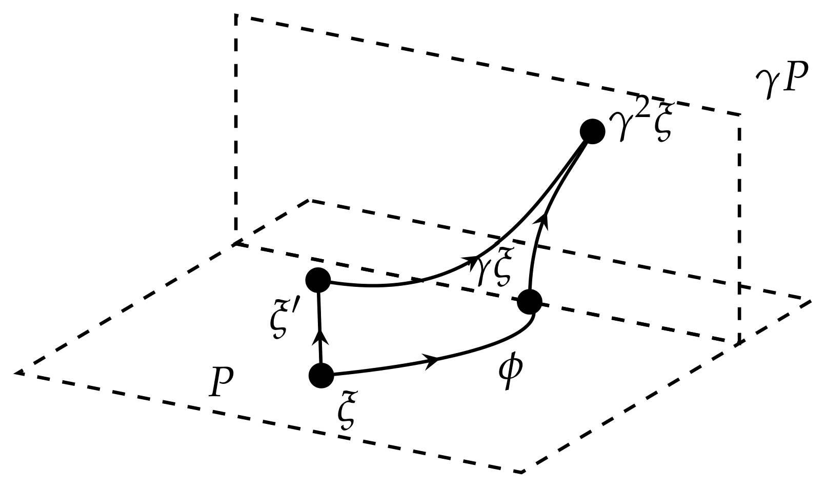
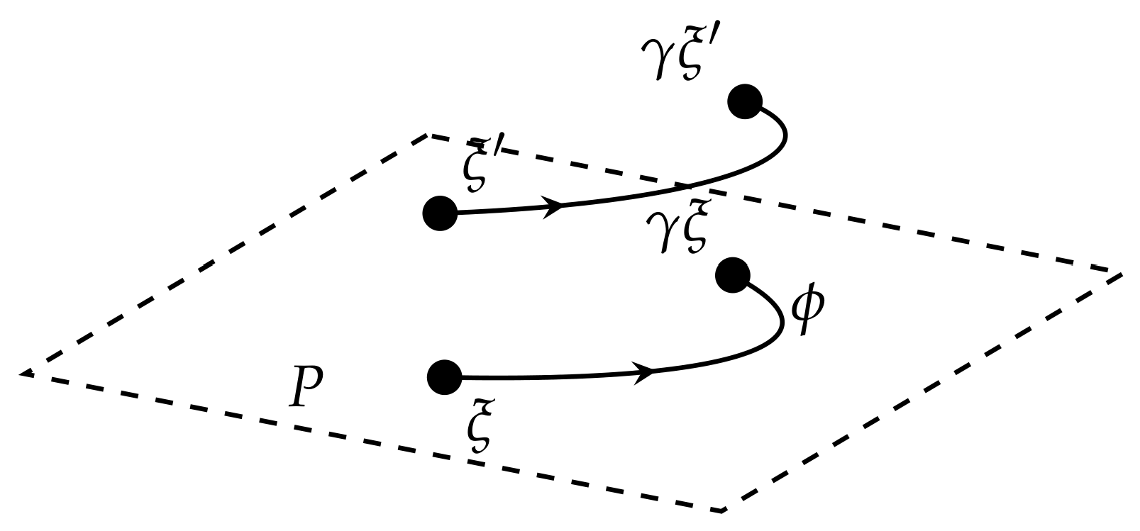
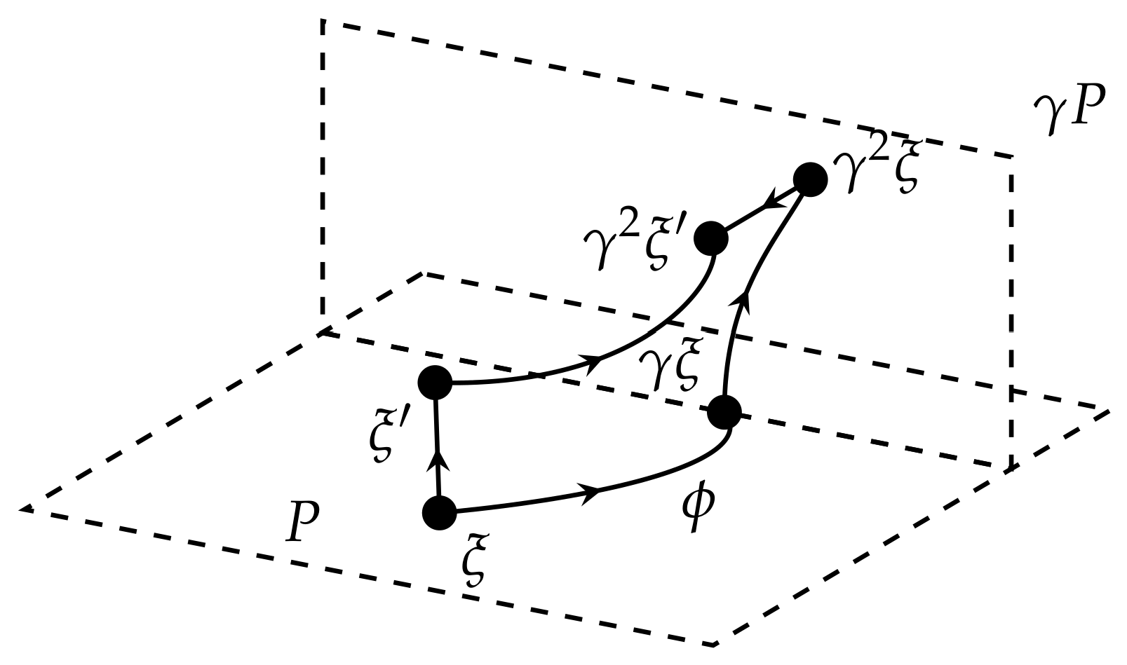
The schematic diagrams of the two kinds of new heteroclinic trajectories in Theorem 1 and Theorem 2 are shown in Figure 1 and Figure 2. Figure 3 and Figure 4 depict the two kinds of new heteroclinic connections in Theorem 3.

5. Transverse Bifurcation of Type A

Here we study transverse bifurcations for homoclinic cycles of type A . Our aim is to demonstrate that when a transverse bifurcation takes place, it gives rise to periodic solutions originating from the cycle.
The classification of Type A homoclinic cycles in R 5 is as follows:
  • For dim P = 3 : 2-[12].
  • For dim P = 2 : 3-[123].
Lemma 6.
For type A homoclinic cycles, the isotropy subgroup of the invariant plane P is Σ Z 2 . Its generator σ acts trivially on P and as −id on P .
Proof. 
According to Definition 5, every element of Σ acts in the same way on each eigenspace of d f ( ξ ) within P . If an element σ Σ acts as multiplication by 1 on one transverse eigenspace, then it must act as 1 on all the remaining eigenspaces. Thus, σ is precisely the required nontrivial element, and its uniqueness is ensured by the distinctness of the eigenvalues of d f ( ξ ) .    ☐
Consider the cross sections H i n and H o u t together with the Poincaré map g = γ 1 ψ φ defined in Section 3 for a homoclinic cycle X. Let x ( t ) be a periodic solution of system (1) lying in a sufficiently small neighborhood of X. Assume that x ( t ) intersects γ i H i n for every integer i > 1 and choose x ( 0 ) H i n . We say that x ( t ) is k periodic if there exists an integer k > 1 such that
g k ( x ( 0 ) ) Γ x ( 0 ) ,
and
g i ( x ( 0 ) ) Γ x ( 0 ) , i = 1 , 2 , , k 1
(see [6]). Because H i n is a small cross section, if some δ Γ satisfies δ x ( 0 ) H i n , then necessarily δ H i n = H i n . The following lemma is adapted from Proposition 4.3 of [6]; the proof remains the same.
Lemma 7.
Suppose δ Γ . Then
δ H i n = H i n iff δ = id or δ = γ 1 σ γ .
This lemma implies if δ x ( 0 ) H i n , then δ = id or δ = γ 1 σ γ .
Notice that if a k periodic solution x ( t ) satisfies
g k x ( 0 ) = γ 1 σ γ x ( 0 ) ,
then x ( t ) actually lies in a small neighborhood of a homoclinic cycle different from X. In particular, if x ( 0 ) is a fixed point of γ 1 σ γ g , then x ( t ) is a 1-periodic solution close to the homoclinic cycle that contains the equilibria ( σ γ ) i ξ for i = 1 , 2 , 3 , . Therefore, we restrict our attention to the case where the coefficient a 44 0 for both type 2-[12] and type 3-[123]; this condition will be shown to produce a fixed point of g in the following subsections. Otherwise, we simply replace γ by σ γ .

5.1. Type 2-[12] Cycles

In this subsection, we study the homoclinic cycle X under the following nondegeneracy conditions:
r 1 ( 0 , 0 ) > 0 , r 2 ( 0 , 0 ) > 0 , c ( 0 , 0 ) > e ( 0 , 0 ) > 0 , t ( 0 ) = 0 , t ( 0 ) > 0 , a 34 0 , a 44 > 0 , a 44 1 .
Theorem 4.
Assume X is of type 2-[12]. If the nondegeneracy conditions (15) hold, and the real parts of all eigenvalues at ξ (except t ( λ ) ) satisfy a nonresonance condition up to a sufficiently high order N, then, for sufficiently small | λ | , a unique 1-periodic solution bifurcates from X with the properties:
(a) 
if 0 < a 44 < 1 , the bifurcation occurs for λ > 0 , and the periodic solution is asymptotically stable;
(b) 
if a 44 > 1 , the bifurcation occurs for λ < 0 , and the periodic solution is unstable.
Proof. 
We reparameterize so that t ( λ ) λ and set
c ( 0 , λ ) = c 0 , e ( 0 , λ ) = e 0 , r 1 ( 0 , λ ) = r 10 , r 2 ( 0 , λ ) = r 20
as in Section 3.
We seek a fixed point ( u 1 , u 2 , w , z ) of the Poincaré map g ( u 1 , u 2 , w , z ) , which satisfies
g ( u 1 , u 2 , w , z ) = ( u 1 , u 2 , w , z ) .
In the ( u 1 , u 2 ) coordinates the equations read
F 1 ( u 1 , u 2 , w , z ) = u 1 η 1 ( u 1 , u 2 , w , z , λ ) = 0 , F 2 ( u 1 , u 2 , w , z ) = u 2 η 2 ( u 1 , u 2 , w , z , λ ) = 0 .
Recalling the construction of Poincaré map g from Section 3, we directly obtain
F 1 u 1 F 1 u 2 F 2 u 1 F 2 u 2 = 1 at ( u 1 , u 2 , w , z , λ ) = ( 0 , 0 , 0 , 0 , 0 ) .
Since the Jacobian determinant is nonzero, the implicit function theorem guarantees a unique local solution, which we write as
( u 1 , u 2 ) = ( η 1 * ( w , z , λ ) , η 2 * ( w , z , λ ) ) ,
where η 1 * , η 2 * are smooth in their arguments. Substituting this into the equations for the w and z coordinates yields the reduced system:
w = a 33 w c 0 e 0 + a 34 z w λ e 0 + ω 4 ( u 1 , u 2 , w , z ) , z = a 43 w c 0 e 0 + a 44 z w λ e 0 + ω 5 ( u 1 , u 2 , w , z ) .
For λ 0 , we introduce new variables
τ = w λ e 0 , ρ = z w .
Then (18) becomes
τ e 0 λ = a 33 τ c 0 λ + a 34 ρ τ e 0 λ 1 + ω 4 ( η 1 * , η 2 * , τ e 0 λ , ρ τ e 0 λ ) , ρ τ e 0 λ = a 43 τ c 0 λ + a 44 ρ τ e 0 λ 1 + ω 5 ( η 1 * , η 2 * , τ e 0 λ , ρ τ e 0 λ ) .
The functions ω 4 and ω 5 have the following asymptotic forms:
ω 4 ( η 1 * , η 2 * , τ e 0 λ , ρ τ e 0 λ ) = τ c 0 λ O ( ρ τ e 0 λ ) + ρ τ e 0 λ 1 O ( ρ τ e 0 λ ) + O ( ( τ c 0 λ , ρ τ e 0 λ 1 ) ( τ c 0 λ , ρ τ e 0 λ 1 , τ r 10 λ , τ r 20 λ ) k 1 ) , ω 5 ( η 1 * , η 2 * , τ e 0 λ , ρ τ e 0 λ ) = τ c 0 λ O ( ρ τ e 0 λ ) + ρ τ e 0 λ 1 O ( ρ τ e 0 λ ) + O ( ( τ c 0 λ , ρ τ e 0 λ 1 ) ( τ c 0 λ , ρ τ e 0 λ 1 , τ r 10 λ , τ r 20 λ ) k 1 ) ,
where k 2 .
Multiplying both sides of Equations (19) by τ 1 e 0 λ yields the transformed system
τ = a 33 τ c 0 e 0 λ + 1 + a 34 ρ + τ 1 e 0 λ ω 4 ( η 1 * , η 2 * , τ e 0 λ , ρ τ e 0 λ ) , ρ τ = a 43 τ c 0 e 0 λ + 1 + a 44 ρ + τ 1 e 0 λ ω 5 ( η 1 * , η 2 * , τ e 0 λ , ρ τ e 0 λ ) .
We now rewrite system (20) in the more compact form
τ a 34 ρ + Ω ( τ 1 λ ) = 0 , ρ τ a 44 ρ + Ω ¯ ( τ 1 λ ) = 0 .
where Ω ( τ 1 λ ) , Ω ¯ ( τ 1 λ ) denotes functions whose leading terms are of order
τ C 0 λ , C 0 = min { e 0 , c 0 e 0 } .
together with all remaining higher-order contributions.
Since 0 < w 1 , 0 < τ < 1 for λ > 0 and τ > 1 for λ < 0 . It is obvious that there is no solution for λ < 0 when 0 < a 44 < 1 and no solution for λ > 0 when a 44 > 1 .
Now we begin with the case 0 < a 44 < 1 . To analyze the behavior near λ = 0 , we smoothly extend the function τ 1 λ originally defined for λ > 0 to λ 0 by setting τ 1 λ = 0 for λ 0 . We still denote this extended function by τ 1 λ , so that Equations (21) keep the same form.
Applying the implicit function at the point ( τ , ρ , λ ) = ( a 44 , a 44 a 34 , 0 ) gives, for sufficiently small λ , a unique solution
τ = a 44 + o ( 1 ) , ρ = a 44 a 34 + o ( 1 ) .
Returning to the original variables ( w , z ) = ( τ e 0 / λ , ρ τ e 0 / λ ) , we obtain
w = a 44 e 0 λ + o ( a 44 e 0 λ ) , z = a 44 a 34 a 44 e 0 λ + o ( a 44 e 0 λ ) .
Hence, for 0 < a 44 < 1 , a unique 1 periodic solution bifurcates from the homoclinic cycle.
For the case a 44 > 1 , we consider the solution of (21) for λ < 0 . We extend the function τ 1 λ originally defined for λ < 0 smoothly to λ 0 by setting τ 1 λ = 0 for λ 0 . The analysis then proceeds analogously to the case 0 < a 44 < 1 , yielding a unique 1 periodic solution for λ < 0 with the same asymptotic form as given in (23).
We now consider the stability of the 1 periodic solution. The linearization of the Poincaré map at the solution ( u 1 , u 2 , w , z ) is given by
D g | ( u 1 , u 2 , w , z ) = B 1 B 3 0 B 2
where
B 1 = a 11 w r 10 e 0 a 12 w r 20 e 0 a 21 w r 10 e 0 a 22 w r 20 e 0 + h . o . t . ,
and
B 2 = a 33 c 0 e 0 w c 0 e 0 e 0 a 34 λ e 0 z w λ e 0 1 a 34 w λ e 0 a 43 c 0 e 0 w c 0 e 0 e 0 a 44 λ e 0 z w λ e 0 1 a 44 w λ e 0 + h . o . t . ,
with h.o.t. denoting matrices whose entries consist entirely of higher-order terms.
Substituting the fixed point ( u 1 , u 2 , w , z ) given by (23) into the matrices B 1 and B 2 , and discarding terms that contain positive powers of a 44 1 λ , we obtain
B 1 = 0
and
B 2 = λ e 0 a 34 a 44 λ e 0 a 44 a 34 1 .
Notice det B 2 = 0 and Tr ( B 2 ) = 1 λ e 0 . Consequently, the eigenvalues of B 1 are both close to 0, while those of B 2 are approximately 0 and 1 λ e 0 . It follows that for 0 < a 44 < 1 and small λ > 0 , the quantity 1 λ e 0 lies inside the unit circle, so the periodic solution is asymptotically stable. For a 44 > 1 and λ < 0 (small | λ | ), we have 1 λ e 0 > 1 , and the periodic solution is unstable.    ☐

5.2. Type 3-[123] Cycles

For the case dim P = 2 , we impose the following nondegeneracy conditions for the homoclinic cycle X:
r ( 0 , 0 ) > 0 , t 1 ( 0 , 0 ) < 0 , c ( 0 , 0 ) > e ( 0 , 0 ) > 0 , t 2 ( 0 ) = 0 , t 2 ( 0 ) > 0 , a 24 0 , a 44 > 0 , a 44 1 .
Theorem 5.
Assume X is of type 3-[123]. If the nondegeneracy conditions (24) hold, and the real parts of all eigenvalues at ξ (except t 2 ( λ ) ) satisfy a nonresonance condition up to a sufficiently high order N, then, for sufficiently small | λ | , a unique 1 periodic solution bifurcates from X with the properties:
(a) 
if 0 < a 44 < 1 , the bifurcation occurs for λ > 0 , and the periodic solution is asymptotically stable;
(b) 
if a 44 > 1 , the bifurcation occurs for λ < 0 , and the periodic solution is unstable.
Proof. 
We reparameterize so that t 2 ( λ ) λ and set
c ( 0 , λ ) = c 0 , e ( 0 , λ ) = e 0 , r ( 0 , λ ) = r 0 , t 1 ( 0 , λ ) = t 10 .
We seek a fixed point ( u , w , z 1 , z 2 ) of the Poincaré map g ( u , w , z 1 , z 2 ) , which satisfies
g ( u , w , z 1 , z 2 ) = ( u , w , z 1 , z 2 ) .
In the u coordinate equation reads
u = η ( u , w , z 1 , z 2 , λ ) .
Applying the implicit function theorem, we obtain a solution of the form
u = η * ( w , z 1 , z 2 , λ ) ,
where η * is a smooth function of its arguments.
Substituting this expression into the equations for the w , z 1 , z 2 coordinates gives
w = a 22 w c 0 e 0 + a 23 z 1 w t 10 e 0 + a 24 z 2 w λ e 0 + ω 1 ( η * , w , z 1 , z 2 ) , z 1 = a 32 w c 0 e 0 + a 33 z 1 w t 10 e 0 + a 34 z 2 w λ e 0 + ω 2 ( η * , w , z 1 , z 2 ) , z 2 = a 42 w c 0 e 0 + a 43 z 1 w t 10 e 0 + a 44 z 2 w λ e 0 + ω 3 ( η * , w , z 1 , z 2 ) ,
Since t 10 < 0 and c 0 > e 0 , by using the asymptotic form of ω 2 ( w , z 1 , z 2 ) given in Section 3, in a neighborhood of ( w , z 1 , z 2 , λ ) = ( 0 , 0 , 0 , 0 ) , we obtain the asymptotic expression for z 1 = z 1 ( w , z 2 , λ ) as follows:
z 1 = a 32 w c 0 e 0 + a 34 z 2 w λ e 0 + w c 0 e 0 O ( z 2 ) + z 2 w λ e 0 O ( z 2 ) + O w c 0 e 0 , z 2 w λ e 0 w r 0 e 0 , w c 0 e 0 , z 2 w λ e 0 k 1 1 a 33 w t 10 e 0 w t 10 e 0 O ( z 2 ) + w t 10 e 0 O w c 0 e 0 , z 2 w λ e 0 w r 0 e 0 , w c 0 e 0 , z 2 w λ e 0 k 1 = a 32 w c 0 e 0 + a 34 z 2 w λ e 0 + ω 6 ( w , z 2 ) , k 2 ,
where ω 6 ( w , z 2 ) has the asymptotic form
ω 6 ( w , z 2 ) = w c 0 e 0 O ( z 2 ) + z 2 w λ e 0 O ( z 2 ) + O w c 0 e 0 , z 2 w λ e 0 w r 0 e 0 , w c 0 e 0 , z 2 w λ e 0 k 1 + O ( w t 10 e 0 ) O ( ( w c 0 e 0 , z 2 w λ e 0 ) k 1 ) , k 2 ,
as ( w , z 2 , λ ) ( 0 , 0 , 0 ) . Notice that all terms in (28) are of higher order than w c 0 e 0 or z 2 w λ e 0 . Moreover, the expression z 1 w t 10 e 0 can be estimated as
z 1 w t 10 e 0 = w c 0 e 0 O ( w t 10 e 0 ) + z 2 w λ e 0 O ( w t 10 e 0 ) + O ( w t 10 e 0 ) O ( ( w c 0 e 0 , z 2 w λ e 0 ) k ) .
Consequently, for k 1 ,
O ( ( w c 0 e 0 , z 1 w t 10 e 0 , z 2 w λ e 0 ) k ) = O ( ( w c 0 e 0 , z 2 w λ e 0 ) k ) .
Substituting this expression for z 1 from (28) into the equations for w and z 2 yields the reduced system
w = a 22 w c 0 e 0 + a 24 z 2 w λ e 0 + ω ¯ 1 ( w , z 2 ) , z 2 = a 42 w c 0 e 0 + a 44 z 2 w λ e 0 + ω ¯ 3 ( w , z 2 ) ,
where
ω ¯ 1 = w c 0 e 0 O ( z 2 ) + z 2 w λ e 0 O ( z 2 ) + O w c 0 e 0 , z 2 w λ e 0 w r 0 e 0 , w c 0 e 0 , z 2 w λ e 0 k 1 + w c 0 e 0 O ( w t 10 e 0 ) ( 1 + O ( z 2 ) ) + z 2 w λ e 0 O ( w t 10 e 0 ) ( 1 + O ( z 2 ) ) ω ¯ 3 = w c 0 e 0 O ( z 2 ) + z 2 w λ e 0 O ( z 2 ) + O w c 0 e 0 , z 2 w λ e 0 w r 0 e 0 , w c 0 e 0 , z 2 w λ e 0 k 1 + w c 0 e 0 O ( w t 10 e 0 ) ( 1 + O ( z 2 ) ) + z 2 w λ e 0 O ( w t 10 e 0 ) ( 1 + O ( z 2 ) ) , k 2 .
The following analysis is analogous to the proof of Theorem 4. For λ 0 , we introduce new variables
τ = w λ e 0 , ρ = z 2 w ,
and multiply each side of Equations (29) by τ 1 e 0 λ . This gives the system
τ = a 22 τ c 0 e 0 λ + 1 + a 24 ρ + τ 1 e 0 λ ω ¯ 1 ( τ e 0 λ , ρ τ e 0 λ ) , ρ τ = a 42 τ c 0 e 0 λ + 1 + a 44 ρ + τ 1 e 0 λ ω ¯ 3 ( τ e 0 λ , ρ τ e 0 λ ) ,
From (28), the functions ω ¯ 1 and ω ¯ 3 have the following asymptotic forms:
ω ¯ 1 = τ c 0 λ O ( ρ τ e 0 λ ) + ρ τ e 0 λ 1 O ( ρ τ e 0 λ ) + O ( ( τ c 0 λ , ρ τ e 0 λ 1 ) ( τ r 0 λ , τ c 0 λ , ρ τ e 0 λ 1 ) k 1 ) + τ c 0 λ O ( τ t 10 λ ) ( 1 + O ( ρ τ e 0 λ ) ) + ρ τ e 0 λ 1 O ( τ t 10 λ ) ( 1 + O ( ρ τ e 0 λ ) ) ω ¯ 3 = τ c 0 λ O ( ρ τ e 0 λ ) + ρ τ e 0 λ 1 O ( ρ τ e 0 λ ) + O ( ( τ c 0 λ , ρ τ e 0 λ 1 ) ( τ r 0 λ , τ c 0 λ , ρ τ e 0 λ 1 ) k 1 ) + τ c 0 λ O ( τ t 10 λ ) ( 1 + O ( ρ τ e 0 λ ) ) + ρ τ e 0 λ 1 O ( τ t 10 λ ) ( 1 + O ( ρ τ e 0 λ ) ) ,
where k 2 .
We rewrite system (30) in the form
τ = a 24 ρ + Ω ( τ 1 λ ) , ρ τ = a 44 ρ + Ω ¯ ( τ 1 λ ) ,
where Ω ( τ 1 λ ) , Ω ¯ ( τ 1 λ ) denote functions whose leading terms are of order
τ C 0 λ , C 0 = min { e 0 , c 0 e 0 , t 10 } .
together with all remaining higher-order contributions.
When 0 < a 44 < 1 , we consider the solution for λ > 0 . After uniquely extending the function τ 1 λ (defined for λ > 0 ) to λ 0 and applying the implicit function theorem at ( τ , ρ , λ ) = ( a 44 , a 44 a 24 , 0 ) , we obtain a unique solution ( τ ( λ ) , ρ ( λ ) ) :
τ = a 44 + o ( 1 ) , ρ = a 44 a 24 + o ( 1 ) .
Tracking back through the substitutions, we derive the unique 1 periodic solution
w = a 44 e 0 λ + o ( a 44 e 0 λ ) , z 1 = a 34 a 24 a 44 e 0 λ + o ( a 44 e 0 λ ) , z 2 = a 44 a 24 a 44 e 0 λ + o ( a 44 e 0 λ ) .
For the case when a 44 > 1 , we consider the solution for λ < 0 . By extending the function τ 1 λ (defined for λ < 0 ) uniquely to λ 0 , the analysis is similar to the case 0 < a 44 < 1 and the solution takes the same form.
Next, we consider the stability of the 1 periodic solution. Linearizing the Poincaré map at the solution ( u , w , z 1 , z 2 ) yields
D g | ( u 1 , w , z 1 , z 2 ) = a 11 w r 0 e 0 + o ( w r 0 e 0 ) b 3 0 B 2
where
B 2 = a 22 c 0 e 0 w c 0 e 0 1 a 23 z 1 t 10 e 0 w t 10 e 0 1 a 24 z 2 λ e 0 w λ e 0 1 a 23 w t 10 e 0 a 24 w λ e 0 a 32 c 0 e 0 w c 0 e 0 1 a 33 z 1 t 10 e 0 w t 10 e 0 1 a 34 z 2 λ e 0 w λ e 0 1 a 33 w t 10 e 0 a 34 w λ e 0 a 42 c 0 e 0 w c 0 e 0 1 a 43 z 1 t 10 e 0 w t 10 e 0 1 a 44 z 2 λ e 0 w λ e 0 1 a 43 w t 10 e 0 a 44 w λ e 0 + h . o . t . ,
with h.o.t. denoting matrices whose entries consist entirely of higher-order terms.
Substituting the fixed point given by (33) into the matrix B 2 , and discarding terms that contain positive powers of a 44 1 λ , we obtain
B 2 = λ e 0 0 a 24 a 44 a 34 a 24 λ e 0 0 a 34 a 44 a 44 a 24 λ e 0 0 1
The three eigenvalues of B 2 are
m 1 , 2 = 0 , m 3 = 1 λ e 0 .
Consequently, for 0 < a 44 < 1 and small λ > 0 , we have m 1 , 2 , 3 < 1 ; hence the periodic solution is asymptotically stable. For a 44 > 1 and small | λ | with λ < 0 , we obtain m 3 > 1 , and the periodic solution is unstable.    ☐

5.3. Numerical Simulation

Here are two examples to illustrate the bifurcation behavior predicted by Theorems 4 and 5 in R 5 .
Example 1.
For a cycle of type 2-[12] with dim P = 3 (Theorem 4), we take
x ˙ 1 = x 1 ( 0.5 x 1 2 x 2 2 x 3 2 ) x 1 x 2 + 0.01 x 3 x 5 3 , x ˙ 2 = ( 1 x 2 2 x 1 2 x 3 2 ) x 2 + x 1 2 x 3 2 , x ˙ 3 = x 3 ( 0.5 x 3 2 x 2 2 x 1 2 ) + x 3 x 2 + 0.01 x 1 x 5 3 , x ˙ 4 = 2 x 4 + x 1 2 x 3 2 , x ˙ 5 = λ x 5 x 5 3 ,
where the symmetry group Γ 1 is generated by
σ 1 : ( x 1 , x 2 , x 3 , x 4 , x 5 ) ( x 1 , x 2 , x 3 , x 4 , x 5 ) , γ 1 : ( x 1 , x 2 , x 3 , x 4 , x 5 ) ( x 3 , x 2 , x 1 , x 4 , x 5 ) .
A homoclinic cycle consisting of ξ = ( 0 , 1 , 0 , 0 , 0 ) and γ ξ = ( 0 , 1 , 0 , 0 , 0 ) together with their connecting trajectories can be obtained by the method of [35]. The invariant subspace P = { ( x 1 , x 2 , 0 , x 4 , 0 ) } has isotropy group Σ 1 = < σ 1 > , implying the cycle is of Type A . The eigenvalues of d f ( ξ ) are one expanding eigenvalue 0.5, contracting eigenvalue −1.5 and two radial eigenvalues −2, and a transverse eigenvalue λ which plays the role of the bifurcation parameter. We chose the parameter values for convenience; a small perturbation of the parameters restores the nonresonance condition without affecting the qualitative behavior of the numerical results.
Example 2.
For a cycle of type 3-[123] with dim P = 2 (Theorem 5), we take
x ˙ 1 = x 1 ( 0.5 x 1 2 x 2 2 x 3 2 ) x 1 x 2 + 0.01 x 3 ( x 4 3 + x 5 3 ) , x ˙ 2 = ( 1 x 2 2 x 1 2 x 3 2 ) x 2 + x 1 2 x 3 2 , x ˙ 3 = x 3 ( 0.5 x 3 2 x 2 2 x 1 2 ) + x 3 x 2 + 0.01 x 1 ( x 4 3 + x 5 3 ) , x ˙ 4 = 2 x 4 , x ˙ 5 = λ x 5 x 5 3 ,
where the symmetry group Γ 2 is generated by
σ 2 : ( x 1 , x 2 , x 3 , x 4 , x 5 ) ( x 1 , x 2 , x 3 , x 4 , x 5 ) , γ 2 : ( x 1 , x 2 , x 3 , x 4 , x 5 ) ( x 3 , x 2 , x 1 , x 4 , x 5 ) .
The same argument as for system (35) yields the existence of a homoclinic cycle of type A .
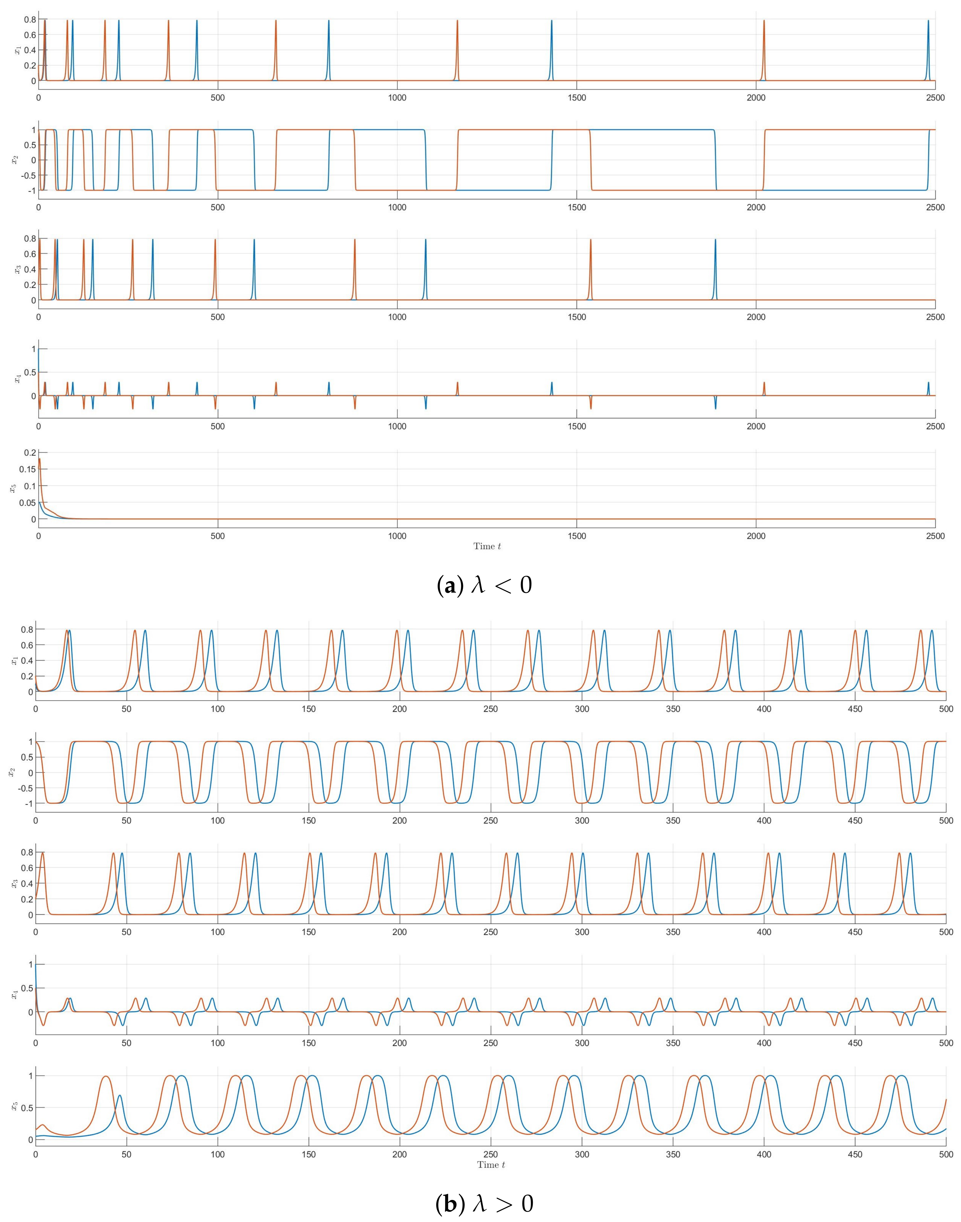
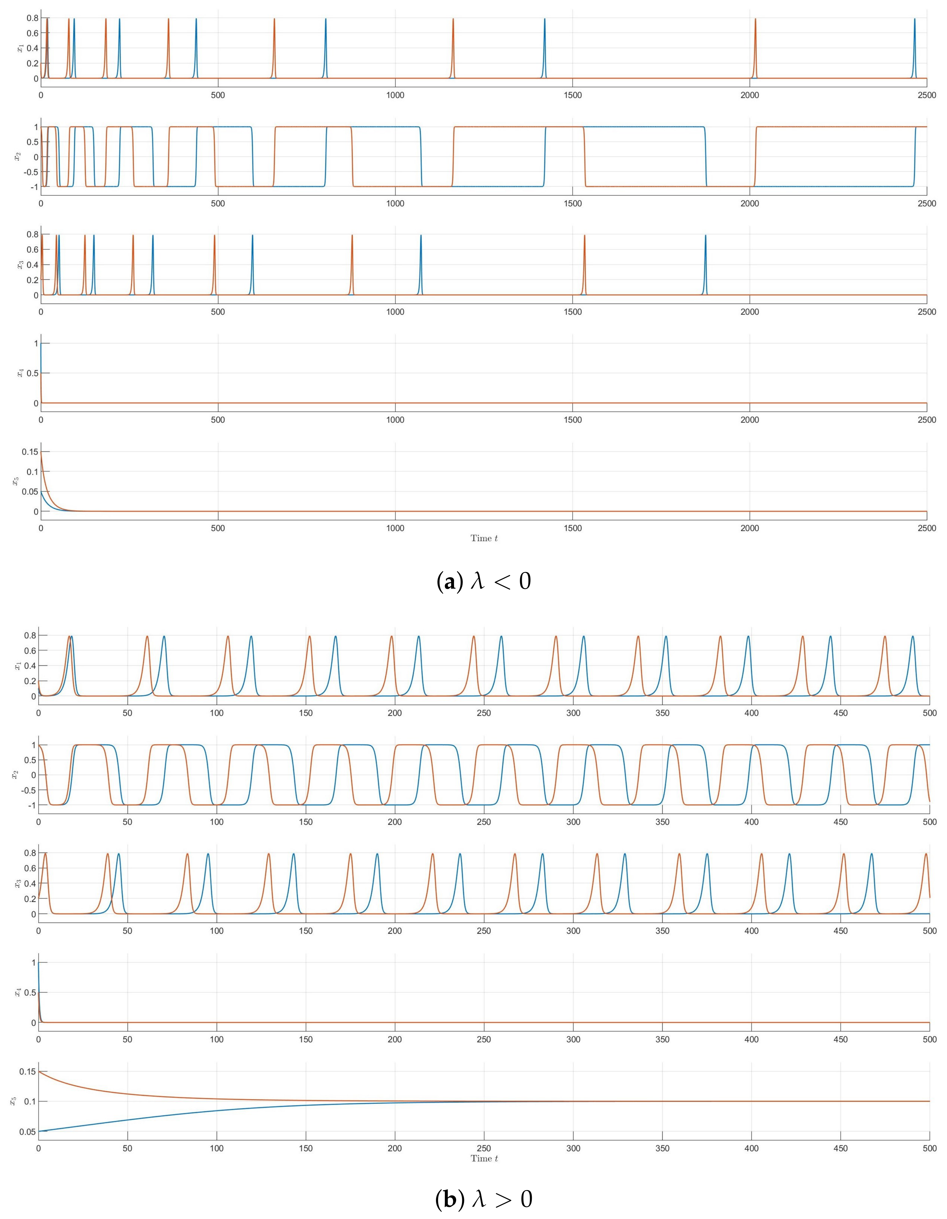
We solve each system on both sides of the bifurcation and display the time series of the state variables in Figure 5 and Figure 6. For each system we integrate with the two initial conditions
IC 1 = ( x 1 ( 0 ) , , x 5 ( 0 ) ) = ( 0.1 , 1 , 0.2 , 1 , 0.05 ) , IC 2 = ( x 1 ( 0 ) , , x 5 ( 0 ) ) = ( 0.2 , 1 , 0.2 , 0.5 , 0.15 ) ,
for the parameter values λ = 0.05 < 0 and λ = 0.01 > 0 , respectively, and the curves obtained from both initial conditions are displayed in each panel of the figures. The time series exhibit a clear contrast between the two sides of the bifurcation. For λ < 0 the trajectories converge to the homoclinic cycle and display an eruptive, non-regular motion: long intervals of near-stationary behavior near the saddle equilibria are interrupted by abrupt fast excursions along the connecting orbits. For λ > 0 , in contrast, the motion becomes regular and periodic: the trajectories settle onto a stable periodic orbit with a well-defined amplitude and frequency, confirming the emergence of a stable 1-periodic solution bifurcating from the cycle, as predicted by Theorems 4 and 5.

6. Transverse Bifurcation of Type 3-[12][3] and Type 3-[1][23]

For a cycle X of type 3-[12][3], it is confined to a four-dimensional flow-invariant subspace denoted by R 1 . When the bifurcation occurs along the transverse eigenvalue of d f ( ξ ) within R 1 , the behavior is similar to the type A case with dim P = 3 , leading to the emergence of a 1 periodic solution. When the bifurcation occurs along the eigenvalue of d f ( ξ ) outside R 1 , the argument parallels that of the type Z case, resulting in the formation of new homoclinic cycles.
We label the isotypic components by the first component U 1 and the second component U 2 in the same way as in Section 4. Assume the following nondegeneracy conditions are satisfied
r ( 0 , 0 ) > 0 , t 1 ( 0 , 0 ) < 0 , c ( 0 , 0 ) > e ( 0 , 0 ) > 0 , t 2 ( 0 ) = 0 , t 2 ( 0 ) > 0 , h z z z ( 0 , 0 ) < 0 , a 24 0 , a 44 > 0 , a 44 1 ,
Theorem 6.
Assume X is of type 3-[12][3]. If the nondegeneracy conditions (37) hold, and the real parts of all eigenvalues at ξ (except t 2 ( λ ) ) satisfy a nonresonance condition up to a sufficiently high order N, then,
(a) 
if the bifurcation occurs in the second component, a unique 1-periodic solution bifurcates from X for | λ | sufficiently small. Moreover, it is asymptotically stable for 0 < a 44 < 1 and unstable for a 44 > 1 .
(b) 
if the bifurcation occurs in the first component, new asymptotically stable homoclinic cycles bifurcate from X for sufficiently small λ > 0 .
For a cycle X of type 3-[1][23], X is confined to a three-dimensional invariant subspace denoted by Q. By symmetry, the coefficients a 23 and a 24 in the Poincaré map vanish.
When searching for 1-periodic solutions bifurcating from the homoclinic cycle X, following a discussion analogous to that for the type A cycle, one must solve
w = a 22 w c 0 e 0 + o ( w c 0 e 0 ) ,
which yields a contradiction for w close to zero. Hence, no 1 periodic solution exists in a neighborhood of X for small λ . Moreover, because no additional invariant subspaces beyond Q are present, the existence of new homoclinic cycles as λ passes through zero cannot be established.

7. Conclusions

This paper has studied codimension-one transverse bifurcations—where a single transverse eigenvalue crosses zero—for every class of simple robust homoclinic cycles in R 5 . For cycles belonging to the types 2-[1][2], 2-[2][1], 2-[12], 3-[12][3], 3-[1][2][3], and 3-[2][1][3], the transverse bifurcations behave similarly to those of homoclinic cycles in R 4 described in [6], giving rise either to new homoclinic cycles or to a unique 1 periodic solution bifurcating from the original cycle. For cycles of type 3-[123], the emergence of a unique 1 periodic solution has also been established.
For type 3-[1][23], the approach fails for a structural reason: the cycle is confined to a three-dimensional invariant subspace Q, symmetry forces a 23 = a 24 = 0 , and the fixed-point equation for a 1 periodic solution, w = a 22 w c 0 / e 0 + o ( w c 0 / e 0 ) , has no solution near w = 0 ; moreover, with no invariant subspace beyond Q, new homoclinic cycles cannot be established either. This marks the boundary of the Poincaré-map framework and motivates non-symmetric or numerical approaches for this class.
Within this framework, the main assumptions are not merely technical: the nonresonance condition guarantees that the normal-form reduction in Takens [33] and Bonckaert [34] applies, while the eigenvalues conditions keep the connecting dynamics one-dimensional, so that the return map is governed by a single scalar power law and the bifurcation criteria by a single coefficient; their violation would couple radial and transverse dynamics and destroy these explicit criteria. The approach is preferable to GSPT or Melnikov-type methods whenever connections are robust and symmetries are preserved, as it yields uniform criteria for entire classes of cycles without requiring a fast-slow structure; the latter methods become necessary only when connections are non-robust or symmetries are broken.
A natural direction for future work is the simultaneous crossing of a pair of transverse eigenvalues, which would induce a Hopf bifurcation and require a two-dimensional extension of the Poincaré-map construction. Resonant cases, where the nonresonance conditions fail, and the numerical exploration of classes inaccessible to the present framework, such as type 3-[1][23], are further open problems.

Author Contributions

Conceptualization, Y.Z. and C.L.; methodology, Y.Z. and C.L.; formal analysis, Y.Z., C.L. and K.H.; investigation, Y.Z. and C.L.; resources, C.L.; writing—original draft, Y.Z.; writing—review and editing, Y.Z., C.L. and X.W.; visualization, Y.Z. and K.H.; supervision, C.L. and X.W.; project administration, Y.Z.; funding acquisition, C.L. All authors have read and agreed to the published version of the manuscript

Funding

This work is supported by NSFC [Grant No. 62227810].

Data Availability Statement

The original contributions presented in this study are included in the article. Further inquiries can be directed to the corresponding authors.

Conflicts of Interest

The authors declare no conflict of interest.

References

  1. Busse, F.H.; Heikes, K.E. Convection in a Rotating Layer: A Simple Case of Turbulence. Science 1980, 208, 173–175. [Google Scholar] [CrossRef] [Scilit] [PubMed]
  2. Hofbauer, J.; Sigmund, K. The Theory of Evolution and Dynamical Systems; Cambridge University Press: New York, NY, USA, 1988. [Google Scholar]
  3. May, R.M.; Leonard, W.J. Nonlinear aspects of competition between three species. SIAM J. Appl. Math. 1975, 29, 243–253. [Google Scholar] [CrossRef] [Scilit]
  4. Guckenheimer, J.M.; Holmes, P.J. Structurally stable heteroclinic cycles. Math. Proc. Camb. Philos. Soc. 1988, 103, 189–192. [Google Scholar] [CrossRef] [Scilit]
  5. Field, M.J.; Swift, J.W. Stationary bifurcation to limit cycles and heteroclinic cycles. Nonlinearity 1991, 4, 1001–1043. [Google Scholar] [CrossRef] [Scilit]
  6. Chossat, P.; Krupa, M.; Melbourne, I.; Scheel, A. Transverse bifurcations of homoclinic cycles. Phys. D 1997, 100, 85–100. [Google Scholar] [CrossRef] [Scilit]
  7. Sottocornola, N. Robust homoclinic cycles in. Nonlinearity 2003, 16, 1–24. [Google Scholar] [CrossRef] [Scilit]
  8. Krupa, M.; Melbourne, I. Asymptotic stability of heteroclinic cycles in systems with symmetry. Ergod. Theory Dynam. Syst. 1995, 15, 121–147. [Google Scholar] [CrossRef] [Scilit]
  9. Krupa, M. Robust heteroclinic cycles. J. Nonlinear Sci. 1997, 7, 129–176. [Google Scholar] [CrossRef] [Scilit]
  10. Krupa, M.; Melbourne, I. Asymptotic stability of heteroclinic cycles in systems with symmetry. II. Proc. Roy. Soc. Edinb. Sect. A 2004, 134, 1177–1197. [Google Scholar] [CrossRef] [Scilit]
  11. Castro, S.B.S.D.; Lohse, A. Stability in simple heteroclinic networks in. Dyn. Syst. 2014, 29, 451–481. [Google Scholar] [CrossRef] [Scilit]
  12. Lohse, A. Stability of heteroclinic cycles in transverse bifurcations. Phys. D 2015, 310, 95–103. [Google Scholar] [CrossRef] [Scilit]
  13. Kirk, V.; Postlethwaite, C.M.; Rucklidge, A.M. Resonance bifurcations of robust heteroclinic networks. SIAM J. Appl. Dyn. Syst. 2012, 11, 1360–1401. [Google Scholar] [CrossRef] [Scilit]
  14. Podvigina, O.M.; Chossat, P. Simple heteroclinic cycles in. Nonlinearity 2015, 28, 901–926. [Google Scholar] [CrossRef] [Scilit]
  15. Podvigina, O.M.; Chossat, P. Asymptotic stability of pseudo-simple heteroclinic cycles in. J. Nonlinear Sci. 2017, 27, 343–375. [Google Scholar] [CrossRef] [Scilit]
  16. Chossat, P.; Lauterbach, R. Methods in Equivariant Bifurcations and Dynamical Systems; World Scientific Publishing Company: Singapore, 2000; Volume 15. [Google Scholar]
  17. Childress, S.; Soward, A.M. Convection-Driven Hydromagnetic Dynamo. Phys. Rev. Lett. 1972, 29, 837–839. [Google Scholar] [CrossRef] [Scilit]
  18. Driesse, R.; Homburg, A.J. Resonance bifurcation from homoclinic cycles. J. Differ. Equ. 2009, 246, 2681–2705. [Google Scholar] [CrossRef] [Scilit]
  19. Sottocornola, N. Simple homoclinic cycles in low-dimensional spaces. J. Differ. Equ. 2005, 210, 135–154. [Google Scholar] [CrossRef] [Scilit]
  20. Podvigina, O.M. Classification and stability of simple homoclinic cycles in. Nonlinearity 2013, 26, 1501–1528. [Google Scholar] [CrossRef] [Scilit]
  21. Driesse, R.; Homburg, A.J. Essentially asymptotically stable homoclinic networks. Dyn. Syst. 2009, 24, 459–471. [Google Scholar] [CrossRef] [Scilit]
  22. Postlethwaite, C.M.; Dawes, J.H.P. Resonance bifurcations from robust homoclinic cycles. Nonlinearity 2010, 23, 621–642. [Google Scholar] [CrossRef] [Scilit]
  23. Podvigina, O.M. Stability and bifurcations of heteroclinic cycles of type Z. Nonlinearity 2012, 25, 1887–1917. [Google Scholar] [CrossRef] [Scilit]
  24. Jones, C.K.R.T. Geometric singular perturbation theory. In Dynamical Systems; Lecture Notes in Mathematics 1609; Springer: Berlin/Heidelberg, Germany, 1995; pp. 44–118. [Google Scholar]
  25. Kuehn, C. Multiple Time Scale Dynamics. In Applied Mathematical Sciences 191; Springer: Cham, Switzerland, 2015. [Google Scholar]
  26. Grifò, G.; Iuorio, A. Travelling pulses in the Barkley model: A geometric singular perturbation approach. Chaos Solitons Fractals 2025, 201, 117307. [Google Scholar] [CrossRef] [Scilit]
  27. Melnikov, V.K. On the stability of the center for time periodic perturbations. Trans. Mosc. Math. Soc. 1963, 12, 1–57. [Google Scholar]
  28. Lin, X.-B. Using Melnikov’s method to solve Silnikov’s problems. Proc. Roy. Soc. Edinb. Sect. A 1990, 116, 295–325. [Google Scholar]
  29. Grifó, G.; Currò, C.; Valenti, G. Heteroclinic connections in a hyperbolic reaction-transport model for excitable media. Chaos Solitons Fractals 2025, 200, 117030. [Google Scholar] [CrossRef] [Scilit]
  30. Grifó, G.; Currò, C.; Valenti, G. Travelling waves in dryland ecology: Continuous and discontinuous connections in a hyperbolic vegetation model. Nonlinear Dyn. 2025, 113, 15295–15319. [Google Scholar] [CrossRef] [Scilit]
  31. Grifó, G.; Currò, C.; Valenti, G. Wavefront propagation in a hyperbolic model of hantavirus infection. Math. Comput. Simul. 2026, 249, 300–322. [Google Scholar] [CrossRef] [Scilit]
  32. Golubitsky, M.; Stewart, I.; Schaeffer, D.G. Singularities and Groups in Bifurcation Theory, Volume II; Applied Mathematical Sciences 69; Springer: New York, NY, USA; Reprinted by World Publishing Corporation: Beijing, China, 1991. [Google Scholar]
  33. Takens, F. Partially hyperbolic fixed points. Topology 1971, 10, 133–147. [Google Scholar] [CrossRef] [Scilit]
  34. Bonckaert, P. Symmetric and reversible families of vector fields near a partially hyperbolic singularity. Ergod. Theory Dynam. Syst. 2000, 20, 1627–1637. [Google Scholar] [CrossRef] [Scilit]
  35. Sandstede, B.; Scheel, A. Forced Symmetry Breaking of Homoclinic Cycles. Nonlinearity 1995, 8, 333–365. [Google Scholar] [CrossRef] [Scilit]
Figure 1. Schematic diagram of the heteroclinic trajectory from ξ to γ ξ .
Mathematics 14 03012 g001
Figure 2. Schematic diagram of the heteroclinic trajectories from ξ to γ 2 ξ .
Mathematics 14 03012 g002
Figure 3. Schematic diagram of the heteroclinic connection ξ ξ γ ξ .
Mathematics 14 03012 g003
Figure 4. Schematic diagram of the heteroclinic connection ξ ξ γ 2 ξ .
Mathematics 14 03012 g004
Figure 5. Numerical simulation for a cycle of type 2-[12] governed by (35): time series of the state variables for (a) λ = 0.05 and (b) λ = 0.01 . The blue and red curves correspond to the initial conditions IC 1 and IC 2 , respectively.
Mathematics 14 03012 g005
Figure 6. Numerical simulation for a cycle of type 3-[123] governed by (36): time series of the state variables for (a) λ = 0.05 and (b) λ = 0.01 . The blue and red curves correspond to the initial conditions IC 1 and IC 2 , respectively.
Mathematics 14 03012 g006
Table 1. Conditions for asymptotic stability in R 5 .
ClassConditions for Asymptotic StabilityType
1-[1] c > e A , Z
2-[12] c > e , t < 0 A
2-[1][2] c > e , t < 0 Z
2-[2][1] c t > e , t < 0 Z
3-[123] c > e , t 1 < 0 , t 2 < 0 A
3-[12][3] c > e , t 1 < 0 , t 2 < 0
3-[1][23] c > e , t 1 < 0 , t 2 < 0
3-[1][2][3] c > e , t 1 < 0 , t 2 < 0 Z
3-[1][3][2] c > e , t 1 < 0 , t 2 < 0 Z
3-[2][1][3] c t 1 > e , t 1 < 0 , t 2 < 0 Z
3-[2][3][1] c t 1 t 2 > e , t 1 < 0 , t 2 < 0 Z
Table 2. Action of the twist γ on the isotypic components of P for each cycle type.
Cycle TypeComponents of P Action of γ
2-[1][2] U 1 U 2 γ U 1 = U 1 , γ U 2 = U 2
2-[2][1] U 1 U 2 γ U 1 = U 2 , γ U 2 = U 1
3-[1][2][3] U 1 U 2 U 3 γ U 1 = U 1 , γ U 2 = U 2 , γ U 3 = U 3
3-[2][1][3] U 1 U 2 U 3 γ U 1 = U 2 , γ U 2 = U 1 , γ U 3 = U 3
3-[2][3][1] U 1 U 2 U 3 γ U 1 = U 3 , γ U 2 = U 1 , γ U 3 = U 2
3-[1][3][2] U 1 U 2 U 3 γ U 1 = U 1 , γ U 2 = U 3 , γ U 3 = U 2
Disclaimer/Publisher’s Note: The statements, opinions and data contained in all publications are solely those of the individual author(s) and contributor(s) and not of MDPI and/or the editor(s). MDPI and/or the editor(s) disclaim responsibility for any injury to people or property resulting from any ideas, methods, instructions or products referred to in the content.