


Abstract
The biological interfaces encountered by ultrasound are rarely welded in the ideal elastic sense. Around tissue–implant contacts, fibrotic capsules, thin membranes, hydrated layers, and tissue-mimicking phantoms, a weak boundary may involve finite mechanical compliance, viscoelastic memory, and local thermo-diffusive exchange. Here, we develop a forward scattering model for a plane P-wave incident from an elastic half-space onto a fractional bio-thermo-diffusive viscoelastic half-space through such an imperfect interface. Caputo-type memory is used in the viscoelastic moduli and the thermal and diffusive relaxation terms, while normal and tangential spring-layer laws describe the mechanical weakness of the contact. The formulation gives a coupled longitudinal dispersion matrix and a reduced six-amplitude interface system. In the revised flux calculation, mechanical reflection and transmission are obtained from the signed total stress–velocity work of the complete reflected and transmitted fields, so modal cross-contributions are retained. The accepted computational population contains 1326 paths and 131,361 points from sub-kilohertz frequencies to ten megahertz, with high-precision recomputation and reliability grades used where conditioning requires caution. Thermochemical quantities remain separate diagnostic channels because a physical absorption coefficient cannot be identified from the present source model. The results show parameter-dependent associations with fractional order, interface stiffness, and frequency, but they do not establish single-parameter causation. The model is therefore intended as a verification-oriented framework for future calibrated studies of weak biological interfaces, not as an experimentally validated or patient-specific predictor.
Keywords:
fractional thermoelasticity; Caputo derivative; imperfect interface; wave scattering; bio-viscoelasticity; signed total-field mechanical flux; cross-terms; conditioning; mass diffusion MSC:
74J20; 35R11; 74F05; 74S40; 80A19
1. Introduction
The ultrasound scattering at soft biological interfaces is often more delicate than the familiar textbook picture of reflection from a perfectly welded elastic boundary. Real contacts are rarely that clean. They may be mechanically weak, thermally imperfect, chemically active, and dispersive in their rheological response, sometimes within the same narrow interfacial region.
The same issue arises in several biomedical and experimental settings. Tissue–implant contacts, fibrotic capsules around foreign bodies, membrane-like tissue barriers, adhesion defects, and hydrated boundaries in tissue-mimicking phantoms all depart from the ideal bonded interface. If perfect bonding is assumed too early, the role of interfacial compliance can be hidden. A change in reflected amplitude may then be interpreted as a simple bulk impedance effect, even when the interface is carrying part of the response.
Fractional viscoelastic models are useful here because they represent distributed relaxation and power-law memory with a relatively small set of parameters. In this work, the Caputo derivative is used for a practical reason: it preserves the usual interpretation of classical initial conditions while allowing hereditary behavior to enter the constitutive response. In the harmonic setting considered below, this choice also keeps the link between fractional memory and frequency-dependent viscoelastic moduli relatively transparent. Other fractional operators may be more suitable for other types of memory. For the present frequency-domain description of soft tissue relaxation, however, the Caputo form gives a controlled first model.
The Caputo source is retained as the primary definition and constitutive memory reference, while causal all-frequency wave behavior is treated as a separate question [1,2]. The substitution is used only after the transient part has decayed: the fields are assumed to be in a long-time periodic state, with zero prehistory or an equivalent steady-state preparation. This restriction is now stated explicitly because the finite lower-terminal transform is not an unconditional identity.
The ingredients of the formulation are established in separate strands of the literature. Generalized thermoelasticity and fractional thermoelastic diffusion provide the bulk background [3,4]. Imperfect mechanical interfaces and two-medium reflection/transmission are also established [5]. The directly closest external study identified in the source-bounded comparison used phase-lag memory, two temperatures, diffusion, and two half-spaces [6]. The authors’ earlier work examined thermo-diffusive viscoelastic reflection and transmission at an imperfect interface [7], and a second related study considered diffusion-linked reflection/transmission in viscoelastic tissue [8]. Other recent models report energy or interaction terms in coupled two-medium problems [9]. These works rule out a first-ever claim for imperfect-interface thermo-diffusive scattering, six scattered amplitudes, or interaction terms.
This contribution is narrower and more precise. The present paper integrates Caputo-type memory, finite mechanical and transport interface laws, signed total-field mechanical , explicit self/cross-term provenance, analytic branch continuation, conditioning-aware precision escalation, and reliability grading in one reproducible scattering workflow. Energy flux theory and quadratic eigenvalue conditioning are known foundations [10,11]; our contribution is their controlled application to this coupled system, not their invention. The biomedical wording is also bounded: experimental fractional-viscoelastic evidence exists [12], but the calculations reported here are not an experimental validation.
The aim is limited but not minor. We do not claim patient-specific prediction from representative parameters. Instead, we construct a forward scattering framework in which the mathematical structure, the mechanical limiting cases, and the calibration requirements are made explicit. This matters for future inverse studies, because bulk acoustic properties, fractional memory, interface stiffness, and transport admittance cannot be inferred safely from a single reflection measurement.
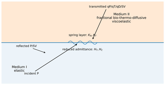
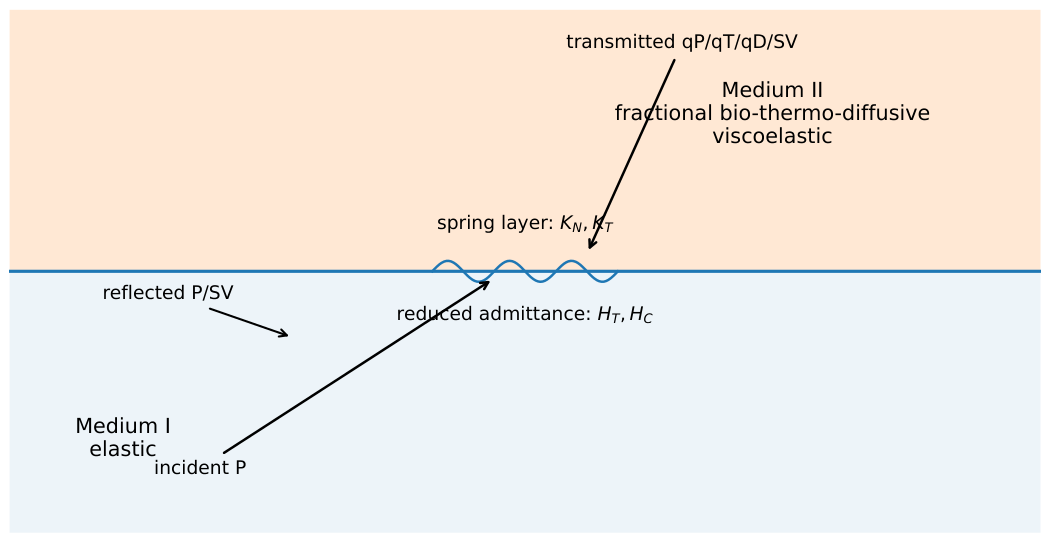
Figure 1 is used as the framework diagram. It identifies the two media, the incident/reflected/transmitted modal content, the mechanical spring layer, and the reduced thermal and chemical exchange laws (see Table 1).
Figure 1.
Framework schematic showing scattering geometry, modal content, mechanical spring layer, and reduced thermochemical interface laws.
Table 1.
Source-bounded comparison used to define this contribution. “Not verified” means that the available authoritative evidence did not support a positive feature claim.
Contributions
The main contributions of this work can be summarized as follows:
- We derive a coupled longitudinal dispersion matrix for the quasi-P, quasi-thermal, and quasi-diffusive branches in a fractional bio-thermo-diffusive viscoelastic half-space under an explicit long-time harmonic assumption and stated common-order and common-relaxation restrictions.
- We formulate a reduced six-amplitude interface system for a plane P-wave incident from a purely elastic half-space. The system includes spring-layer mechanical rows and reduced thermochemical admittance rows, together with analytic branch continuation and normalized eigenvectors.
- We evaluate the mechanical power flux through stress–velocity work using the total fields, including all reflected and transmitted self- and cross-terms. No clipping or forced closure is applied, and the formulation is checked against the relevant elastic limiting cases.
- We report conditioning, residuals, precision escalation, and reliability grades for the accepted population rather than relying on isolated illustrative points.
- We compare the fractional imperfect-interface response with accepted limiting cases, and we interpret frequency and stiffness through the dimensionless groups and , while keeping computational ultrasonic-frequency coverage separate from experimental validation.
- We provide a calibration roadmap linking the model coefficients to measurable inputs from tissue-property databases, phantom experiments, rheometry, elastography, and interface-contact tests, without claiming specimen-level or patient-specific calibration.
2. Mathematical Model
2.1. Geometry and Harmonic Convention
Consider two homogeneous half-spaces separated by the plane . Medium I occupies and is treated as purely elastic. Medium II occupies and is modeled as a fractional bio-thermo-diffusive viscoelastic medium. We restrict the motion to the plane:
All fields are taken to be proportional to
where p denotes the conserved horizontal wavenumber, and q is the vertical wavenumber. For an incident P wave at angle , , with . The elastic Lamé moduli are obtained from the stated density and wave speeds as
These relations are used consistently in the elastic limiting checks.
2.2. Caputo Memory and Fractional Factors
For , the Caputo derivative of a sufficiently smooth scalar is
We assume a long-time steady harmonic state, with the transient associated with the finite lower terminal removed by zero prehistory or equivalent periodic preparation. Under this stated assumption, gives
The temporal branch of the fractional operator is therefore fixed before the spatial radiation condition is imposed. The model uses one order in the viscoelastic, thermal, and diffusive factors. This is a restrictive parameter-reduction assumption, not a universal physical statement. Separate , , and are a direct extension when independent spectra are available.
2.3. Governing Equations in Fractional Medium
The equation of motion is
The fractional heat equation is written as
The fractional diffusion equation is
Here, , , and . The coefficient is kept distinct from the chemoelastic stress coefficient . The stress law in Medium II is
with
The common in the volumetric and shear moduli is another deliberate first-model restriction. It reduces the number of uncalibrated spectral parameters but does not imply that bulk and shear relaxation are identical in tissue. Separate time scales should be used when independent bulk and shear spectra are available. At , the adopted modulus has a Kelvin–Voigt-type frequency dependence; it is not presented as a general integer-order relaxation law.
Causality and passivity are treated as admissibility requirements, not as consequences of the numerical solution. For the chosen harmonic convention, the fractional power is taken on the causal branch, and the constitutive parameters are restricted so that the cycle-averaged material dissipation is non-negative. The accepted calculations also preserve , , , , , and . A complete coupled thermodynamic proof would also require a positive semidefinite heat/mass transport matrix and source-variable choices under which reciprocal cross coefficients satisfy the relevant Onsager symmetry. The present parameterization does not establish that full theorem. We therefore treat , , , , and as calibrated coefficients subject to positivity and reciprocity screening, and we avoid a global thermodynamic-closure claim.
3. Modal Structure and Dispersion Relation
The in-plane displacement field is represented by
For a longitudinal mode,
and substitution gives , with .
where , , , and . The longitudinal roots satisfy ; the SV branch satisfies .
| Entry | Expression | Entry | Expression | Entry | Expression |
The three longitudinal roots are not ordered independently at every point. Starting from a verified seed, each branch is continued through the parameter path by minimizing a composite mismatch in q, phase-aligned eigenvector content, and modal class. Candidate roots are filtered by boundedness and then by outward energy direction; is sufficient for decay but is not used alone to identify a propagating outgoing branch. The longitudinal eigenvectors are normalized with , and their phase is fixed by making the dominant component real and non-negative. The labels quasi-P, quasi-thermal, and quasi-diffusive follow the continued component content rather than a fresh magnitude sort. The computational records retain the root identities for every point. Representative seed labels are the three Stage-C root IDs attached to each accepted parameter case, and transition classes are stored as propagating, attenuating, evanescent, or mixed. Critical transitions are therefore identified from the continued branch and outward-flux status, not from sharp minima in a plotted curve alone. Near a root approach or a large scaled condition number, the solution is recomputed at higher precision, and the point is graded rather than silently discarded.
4. Imperfect Interface System
4.1. Modal Expansion
The scattering unknowns are collected in
For a longitudinal mode m, for transmission and for reflection.
The unit-amplitude interface coefficients are
For an SV mode, , , , , and the thermal/diffusive components vanish.
4.2. Boundary Conditions and Reduced Rows
The mechanical interface is described by traction continuity together with spring-layer displacement jumps:
The reduced thermochemical rows are
These Robin-type conditions represent exchange with reference states on the elastic side that are held at zero perturbation: and . Thus, , and . The chemical driving variable is . It is a reduced interfacial chemical-potential proxy, while the bulk law is written in terms of the concentration gradient. Their compatibility is an adopted linear constitutive reduction; a full chemical-potential formulation would require a free-energy specification and is not claimed here. The six conditions give .
5. Total-Field Mechanical Flux and Thermochemical Reporting
5.1. Total-Field Stress–Velocity Work
For harmonic motion, . On each side of the interface, the total time-averaged mechanical flux is evaluated from the total fields,
Expanding a multimode total field gives the self-terms and all cross-terms. The reflected and transmitted coefficients are
They are signed mechanical coefficients. The symbols , , , , , and remain displacement amplitude coefficients and are never relabeled as energy coefficients. For real spring stiffnesses, the spring layer is mechanically conservative on average. The population-wide balance residual is therefore checked independently from any diagnostic normalization. The accepted residual range is approximately . This residual is a numerical balance check; it is not absorption. We do not clip negative contributions, do not force , and do not define . Physical absorption is not identifiable from the current source model because a complete thermo-mechanical energy balance and an interfacial free-energy law are not present.
5.2. Thermochemical Quantities
The signed thermal and diffusive bilinear quantities are retained, when needed, before any display normalization:
No operation is used in the revised physical results. These quantities are not combined with mechanical R and T through arbitrary weights, and their signs are not suppressed. They remain thermochemical proxies until an independently calibrated free-energy and chemical-potential framework is supplied.
6. Calibration Pathway and Parameter Anchoring
The representative parameters are not intended to reproduce a specific organ, specimen, or patient.
The revision separates parameters that are fixed in the accepted population from those that vary along controlled paths. The only accepted dimensional stiffness value is Pa m−1; the old – stiffness sweep is withdrawn. The compact calibration roadmap is retained, but thermochemical scale factors are no longer used to create physical energy shares (see Table 2).
Table 2.
Calibration roadmap and present interpretation boundary.
7. Numerical Verification and Accepted Results
7.1. Population, Parameter Coverage, and Safeguards
The revised results use the frozen accepted population rather than the earlier private proxy plots. It contains 1326 paths and 131,361 points. The primary orders are ; and are sparse refinement values with 92 points each. The frequency set spans 250 Hz to 10 MHz, including 31.6228 kHz, 100 kHz, 316.228 kHz, 1 MHz, 3.16228 MHz, and 10 MHz as computational ultrasonic-frequency coverage. The accepted dimensional stiffness is Pa m−1. The fixed representative constants inherited from the submitted model are kg m−3, m s−1, m s−1, kg m−3, m s−1, m s−1, W m−1 K−1, J kg−1 K−1, m2 s−1, and K. The dimensionless frequency records correspond to s and s. Coupling and exchange variants are retained through explicit coupling_case and exchange_regime identifiers in the supplied source tables; they are model scenarios, not calibrated tissue constants. The earlier proxy weights are not used in the revised physical results.
The numerical policy reports the full rank, minimum singular value, scaled condition number, relative residual, backward error, precision state, and reliability grade. The descriptive condition bands are <, –, –, and ≥. A total of 68,707 points trigger high precision because of scaled conditioning, and all converge. The final grades are 62,217 Grade A, 68,707 Grade B, and 437 Grade W points. Grade B is retained with escalated-precision provenance; Grade W is retained with an explicit interpretive warning (see Table 3).
Table 3.
Accepted population and numerical-reliability summary.
7.2. Signed Mechanical Coefficients and Selected Angular Path
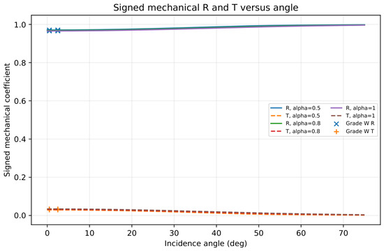
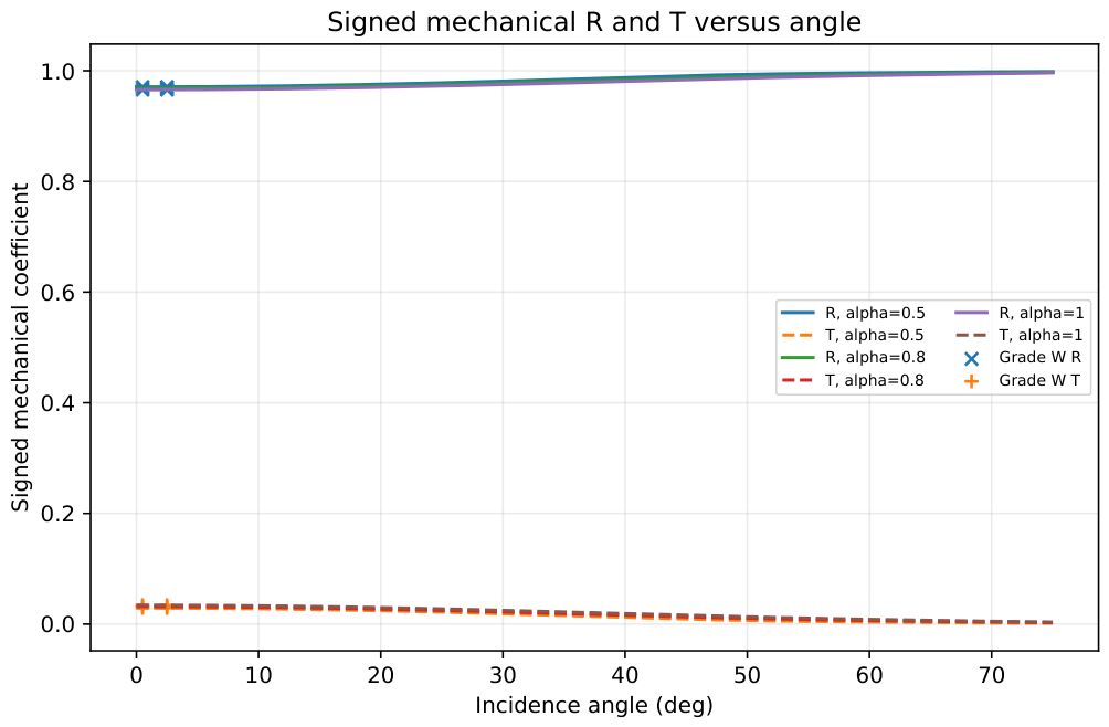
Figure 2 replaces the proxy-normalized angular plots. It is a controlled angle path at 1 kHz with Pa m−1, the frozen exchange case CONTINUITY-KHZ-HT1-HC1, and the baseline coupling case ALL_ZERO. The latter label means that no additional coupling perturbation is applied beyond the stored baseline model coefficients. The path compares the three primary fractional orders while all other recorded path coordinates remain fixed. The total-field R and T values are signed and are not clipped. Small values outside the interval remain linked to residual, cross-term, and precision evidence; they are not converted into a physical absorption coefficient.
Figure 2.
Signed total-field mechanical R and T along the selected angular paths at 1 kHz, with Pa m−1, exchange regime CONTINUITY-KHZ-HT1-HC1, and baseline coupling case ALL_ZERO. No clipping or physical A is used; the six Grade W points are marked.
The accepted population also contains sparse fractional-order refinement paths and a refined frequency path. Those objects are retained in the computational archive, but separate article figures are omitted because their fixed incidence coordinate is not materialized in the frozen path-definition evidence. No coordinate is guessed in this revision.
7.3. Frequency Coverage and Dimensionless Regimes
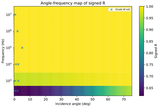
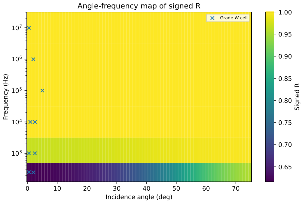
The angle–frequency map in Figure 3 uses six selected accepted frequency slices: 250 Hz, 1 kHz, 10 kHz, 100 kHz, 1 MHz, and 10 MHz. The raw cells are plotted at the actual frequency and angle coordinates with no smoothing or interpolation. This figure is not a full eleven-frequency population average.
Figure 3.
Angle–frequency map of signed R for six selected accepted frequency slices (250 Hz, 1 kHz, 10 kHz, 100 kHz, 1 MHz, and 10 MHz), using raw coordinates without interpolation. Nine Grade W cells are marked.
The dimensionless groups are
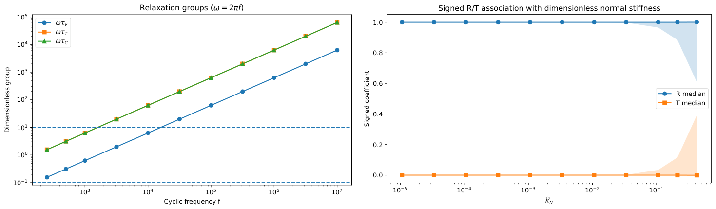
where , and . Figure 4 shows the relaxation groups and the association of the fixed dimensional stiffness with . The dimensional stiffness is not swept. Thus, the displayed dimensionless stiffness changes with frequency and cannot be interpreted as an independent stiffness law.
Figure 4.
Dimensionless interpretation. The left panel gives the accepted relaxation groups. The dashed horizontal lines at and 10 denote descriptive boundaries separating the low (), transitional (), and high () regimes; they are not acceptance thresholds. The right panel shows signed against dimensionless normal stiffness while the dimensional stiffness remains fixed; the association therefore changes with frequency and is not an independent stiffness sweep.
7.4. Cross-Terms and Mechanical Balance
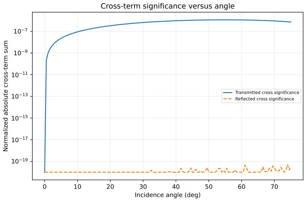
The cross-terms are evaluated from the total fields. Figure 5 reports the absolute reflected and transmitted cross-term significance for the selected path at , 10 kHz, coupling case C14_CROSS_ASYMMETRIC_2, and the baseline angle path. It shows that the cross contribution can be small but non-zero and must remain in the total-field work. Because the plotted ordinate is absolute, the figure does not establish the sign of a cross contribution.
Figure 5.
Absolute reflected and transmitted cross-term significance along the selected baseline angle path at and 10 kHz for coupling case C14_CROSS_ASYMMETRIC_2. The complete signed contributions are retained in the total-field flux; this absolute plot does not show their sign.
The population-wide mechanical residual is independent of any diagnostic normalization and remains at numerical roundoff. Conditioning and reliability diagnostics are reported in Appendix A with their selected path and unequal population limitations.
7.5. Elastic Limiting Checks
In the purely elastic normal-incidence limit, the reflected-P energy coefficient is 0.006361 from both the impedance formula and the numerical formulation; the absolute difference is . The oblique P/SV checks recover the corresponding welded elastic reference when fractional and thermo-diffusive effects are suppressed.
These are limiting benchmarks for the mechanical formulation. They do not validate the coupled biomedical interpretation.
8. Discussion
The central implication of the results is that fractional memory and imperfect contact can interact strongly enough to make oblique reflection more than a simple impedance-contrast problem. The selected accepted paths support this reading, but the associations are not attributed to one scalar parameter and are not treated as specimen-specific calibration. A second implication is methodological. Mechanical reflection and transmission must be calculated from the total stress and velocity fields, with cross contributions retained; thermochemical quantities remain separate diagnostics until an independent calibration fixes their physical scale.
The framework is most relevant when interfacial weakness and material relaxation are expected to occur in the same region. In implant assessment, the spring layer may represent incomplete bonding or local slip. In fibrotic capsules and membrane-like barriers, the reduced admittance rows may represent restricted exchange. For phantom design, the model helps identify which measurements are needed before a phantom can be used to test interface-sensitive ultrasound inversion. For tissue characterization, the same results point toward a combined angular and spectral reading, rather than interpretation from a single measurement. These are proposed interpretation and calibration pathways, not experimentally validated applications.
The spring-layer model should be read as a first-order representation of imperfect contact. It does not attempt to describe roughness, interfacial mass, finite-thickness adhesive layers, or nonlinear contact in full detail. Its role here is more focused: it supplies the simplest mechanically interpretable interface law on which fractional and thermodiffusive effects can be tested. High-frequency scattering, rough interfaces, and finite-thickness coatings would require extensions of this idealization.
The formulation is also linear. It is therefore most appropriate for small-amplitude diagnostic or characterization regimes. Therapeutic ultrasound, high-intensity focused ultrasound, and large-strain deformation may require nonlinear constitutive laws, temperature-dependent properties, perfusion, damage, or finite-strain interface models. Those effects remain outside the scope of the present paper. Still, the scattering structure developed here could provide a useful starting point for such extensions. The accepted calculations include computational coverage into the megahertz range, but no transducer, specimen, or patient data are fitted.
The non-monotonic behavior with fractional order is physically plausible but not attributable to fractional order alone. A change in the common order changes both the magnitude and phase of the complex moduli, the continued roots and modal content, the interface matrix, and the phase relations in total-field work. A local minimum must therefore be read together with branch continuity, cross-terms, scaled conditioning, residual, and precision state.
The stiffness interpretation is narrower than in the submitted manuscript. The accepted population uses one dimensional stiffness value. As frequency changes, the dimensionless stiffness groups change even though the dimensional stiffness does not. The displayed association is useful for regime identification, but it is not an independent stiffness sweep or a monotonic stiffness law.
The closest related literature also narrows the novelty. Imperfect-interface scattering, thermo-diffusive two-medium models, fractional memory, energy terms, and quadratic-eigenvalue methods all predate this work. The contribution is the controlled combination of finite transfer, signed total-field mechanical flux, complete self/cross provenance, branch continuity, precision escalation, reliability grading, and explicit claim boundaries.
9. Relation to Classical Models and Limiting Cases
The formulation recovers several familiar limiting cases:
- gives the integer-order limit of the adopted Kelvin–Voigt-type modulus.
- , suppressed thermodiffusive fields, and recover elastic reflection and transmission.
- recovers perfect mechanical contact.
- and give insulated thermal and diffusive interface conditions.
- approximate reservoir-type temperature and chemical-driving constraints relative to the stated zero perturbation reference states.
Relative to classical imperfect thermoelastic–diffusive interface models, the present framework adds Caputo-type hereditary response and a reliability-controlled total-field flux calculation. Relative to fractional thermoelastic wave models that assume perfect or unspecified contact, it retains spring-layer conditions and finite thermochemical exchange within a directly solvable scattering system. In the common elastic limit, the formulation recovers the classical mechanical benchmarks. Outside that common limit, fractional memory and finite interfacial compliance remain active and can change the reflected and transmitted response. These statements describe a methodological extension, not a universal priority claim.
10. Limitations and Concrete Next Steps
The formulation remains limited by design. It is linear, isotropic, planar, two-dimensional, and restricted to a single incident P wave. It does not include anisotropy, poroelastic flow, finite strain, nonlinear contact, roughness scattering, interfacial mass, finite-thickness coatings, perfusion, active remodeling, or experimentally measured fractional spectra. It also does not derive a physical interfacial storage or dissipation term from a complete thermodynamic potential. The common fractional order and common volumetric/shear relaxation time are additional first-model restrictions. A complete causality/passivity proof for the full coupled system and a calibrated chemical–potential interface law are not supplied. Physical absorption is therefore withheld.
The most important theoretical extension is a thermodynamically grounded interface law. A successor model should introduce an interfacial Helmholtz free energy, derive admissible storage and dissipation from entropy production, and identify , , , and from independent measurements. A biomedical extension would then need to test the framework against tissue-property databases, tissue-mimicking phantoms, and ex vivo tissue measurements.
A practical calibration strategy should not try to fit all parameters at once. A more defensible workflow would first anchor the bulk acoustic and thermal properties, then estimate separate bulk, shear, thermal, and diffusive memory spectra. The continuation and reliability audit should then be repeated without changing the total-field flux definition. Only after these steps should interface stiffness or thermochemical admittance be inferred from angular and spectral measurements with an independently specified transducer geometry.
11. Conclusions
We developed a scattering framework for ultrasonic biological interfaces with fractional memory and imperfect mechanical contact. The model brings together the dispersion relation, the six-amplitude interface system, and the mechanical power-flux calculation in one forward formulation. In the revised calculation, the mechanical coefficients are obtained from total stress–velocity work with all self- and cross-contributions retained. It also avoids adding an empirical residual term just to close the balance, and it does not replace the missing physical absorption coefficient with a balance residual.
The elastic limiting checks support the mechanical part of the model. The accepted angular, frequency, and dimensionless-coordinate records show parameter-dependent associations, but they do not establish single-parameter causation or experimental validation. The reliability records identify where high precision or interpretive warnings are required. The calibration roadmap also shows what would be needed to move from representative simulations toward tissue-specific or phantom-based studies. The model should therefore be read as a theoretical and verification-oriented framework for calibrated studies of weak biological interfaces, not as a finished clinical predictor.
Author Contributions
Conceptualization, A.M.Y.A. and I.S.E.; methodology, A.M.Y.A. and I.S.E.; software, A.M.Y.A.; validation, I.S.E.; formal analysis, A.M.Y.A. and I.S.E.; investigation, A.M.Y.A. and I.S.E.; data curation, A.M.Y.A. and I.S.E.; visualization, A.M.Y.A.; writing—original draft, A.M.Y.A.; writing—review and editing, A.M.Y.A. and I.S.E.; supervision, I.S.E.; funding acquisition, A.M.Y.A. All authors have read and agreed to the published version of the manuscript.
Funding
This research was funded by the Ongoing Research Funding Program, King Saud University, Riyadh, Saudi Arabia, under project number ORF-2026-1780.
Data Availability Statement
No experimental or external datasets were used in this theoretical study. The numerical results supporting the conclusions presented in this article are contained within the article. The underlying machine-readable computational records are retained in a frozen computational archive for traceability, while the private implementation is not publicly released. Further inquiries can be directed to the corresponding authors.
Conflicts of Interest
The authors declare no conflicts of interest.
Abbreviations
The following abbreviations are used in this manuscript:
| Symbol | Definition | Unit | Range/Sign |
| Mass density | kg m−3 | >0 | |
| Longitudinal and shear wave speeds | m s−1 | >0 | |
| Lamé moduli | Pa | , | |
| Common fractional order in the first model | 1 | ||
| Viscoelastic, thermal, and diffusive time scales | s | >0 | |
| Thermal conductivity | W m−1 K−1 | >0 | |
| Specific heat | J kg−1 K−1 | >0 | |
| D | Diffusion coefficient | m2 s−1 | >0 |
| Thermoelastic stress coupling | Pa K−1 | Calibrated | |
| Chemoelastic stress coupling | Pa per concentration unit | Calibrated | |
| Strain–diffusion coupling | Equation-consistent | Calibrated | |
| Heat/mass cross-coupling coefficients | Equation-consistent | Positivity/reciprocity screened | |
| Normal and tangential interface stiffness | Pa m−1 | >0 | |
| Thermal interface conductance | W m−2 K−1 | ≥0 | |
| Diffusive interface conductance | Flux per driving-force unit | ≥0 | |
| Horizontal and vertical wavenumbers | m−1 | Complex q allowed | |
| Signed total-field mechanical coefficients | 1 | Not clipped | |
| Scaled condition number | 1 | Scaling-dependent diagnostic | |
| Relative linear-system residual | 1 | Reported, not used as absorption |
Appendix A. Numerical Reliability and Reporting Boundaries
The accepted population records the rank, minimum singular value, scaled condition number, relative residual, backward error, precision state, and reliability grade at every point. The largest relative residual is ; the balance residual lies within approximately . These quantities support numerical consistency but are not physical absorption measures. The complete machine-readable population and figure source tables are retained in the frozen computational archive used for this revision.
Figure A1 is a selected-path diagnostic, not a population-wide distribution. It uses the same 151-point source path as Figure 5: , 10 kHz, coupling case C14_CROSS_ASYMMETRIC_2, and the baseline angle path. The scaled condition number is algorithmic and scaling-dependent; Grade B points are retained only with converged high-precision provenance.
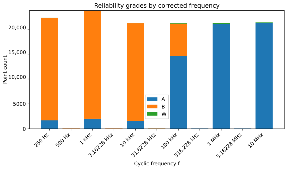
Figure A2 reports raw reliability-grade counts by frequency. The number of populated paths and points is unequal across frequencies, including sparse midpoint frequencies. Bar height alone therefore does not indicate improved or degraded reliability. The count must be read with the corresponding population cardinality and high-precision fraction.
Figure A1.
Selected-pathconditioning and reliability diagnostic at and 10 kHz for coupling case C14_CROSS_ASYMMETRIC_2. The scaled condition number is algorithmic and scaling-dependent; this is not a population-wide distribution.
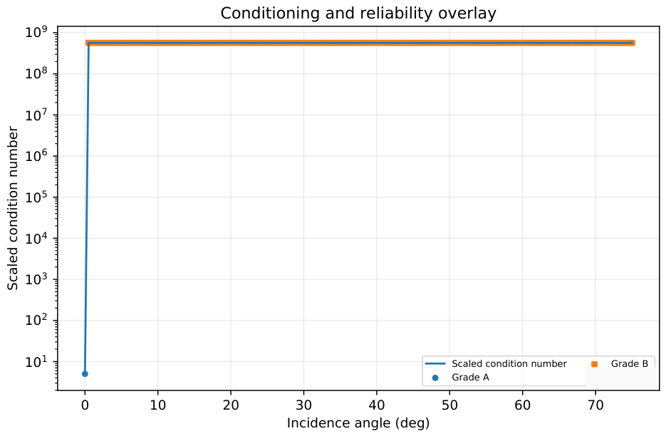
Figure A2.
Raw reliability-grade counts by corrected frequency. Population cardinalities are unequal across frequencies; bar height alone is not a measure of improved or degraded reliability.
Appendix B. Minimal Thermodynamic Closure Template
A fully thermodynamic successor to the present model could begin by assigning an interfacial Helmholtz free energy per unit area. One possible starting form is
where and denote the normal and tangential displacement jumps, and denote the thermochemical jumps, and represents possible internal variables associated with interfacial memory, roughness, damage, or adhesion state. Thermodynamically admissible tractions and exchange laws would then follow from conjugate derivatives of together with non-negative dissipative terms.
The associated entropy production requirement may then be written in the schematic form
where and denote the thermal and diffusive driving forces after a specific thermodynamic choice has been made. The present paper does not impose such a closure, because doing so would require additional experimental information. The template is included only to indicate how a future model could replace the present diagnostic treatment with a first-principles law for interfacial storage and dissipation. No value of is inferred from the numerical balance residual, and no is reported.
References
- Caputo, M. Linear models of dissipation whose Q is almost frequency independent—II. Geophys. J. R. Astron. Soc. 1967, 13, 529–539. [Google Scholar] [CrossRef] [Scilit]
- Holm, S.; Näsholm, S.P. A causal and fractional all-frequency wave equation for lossy media. J. Acoust. Soc. Am. 2011, 130, 2195–2202. [Google Scholar] [CrossRef] [Scilit] [PubMed]
- Lord, H.W.; Shulman, Y. A generalized dynamical theory of thermoelasticity. J. Mech. Phys. Solids 1967, 15, 299–309. [Google Scholar] [CrossRef] [Scilit]
- Xiong, C.; Niu, Y. Fractional-order generalized thermoelastic diffusion theory. Appl. Math. Mech. 2017, 38, 1091–1108. [Google Scholar] [CrossRef] [Scilit]
- Kumar, R.; Sharma, N.; Ram, P. Reflection and transmission of micropolar elastic waves at an imperfect boundary. Multidiscip. Model. Mater. Struct. 2008, 4, 15–36. [Google Scholar] [CrossRef] [Scilit]
- Kaur, I.; Lata, P.; Singh, K. Reflection and refraction of plane wave in piezo-thermoelastic diffusive half spaces with three phase lag memory dependent derivative and two-temperature. Waves Random Complex Media 2022, 32, 2499–2532. [Google Scholar] [CrossRef] [Scilit]
- Abdelaty, A.M.Y.; Lotfy, K.; Sharma, S.; Kumar, R.; Shang, F.; El-Bary, A.A.; Jlali, L.; Elshazly, I.S. Reflection and transmission of thermo-diffusive viscoelastic waves with variable thermal conductivity at an imperfect interface. Struct. Eng. Mech. 2026, 98, 211–234. [Google Scholar] [CrossRef]
- Ghangas, S.; Sharma, S.; Kumar, R.; Abou El Nasr, M.; Lotfy, K.; El-Bary, A.A.; Elshazly, I.S.; Halouani, B. Investigation into viscoelastic tissue under diffusion-related reflection and transmission phenomena. Mech. Res. Commun. 2026, 154, 104659. [Google Scholar] [CrossRef] [Scilit]
- Bibi, F.; Ali, H. Reflection and transmission phenomenon of plane waves at the interface of diffusive viscoelastic porous rotating isotropic medium under Hall current and nonlocal thermoelastic porous solid. J. Strain Anal. Eng. Des. 2024, 59, 491–516. [Google Scholar] [CrossRef] [Scilit]
- Tisseur, F.; Meerbergen, K. The quadratic eigenvalue problem. SIAM Rev. 2001, 43, 235–286. [Google Scholar] [CrossRef] [Scilit]
- Červený, V.; Pšenčík, I. Energy flux in viscoelastic anisotropic media. Geophys. J. Int. 2006, 166, 1299–1317. [Google Scholar] [CrossRef] [Scilit][Green Version]
- Gomez, A.; Callejas, A.; Rus, G.; Saffari, N. Experimental evidence of shear waves in fractional viscoelastic rheological models. Sci. Rep. 2022, 12, 7448. [Google Scholar] [CrossRef] [Scilit] [PubMed]

Disclaimer/Publisher’s Note: The statements, opinions and data contained in all publications are solely those of the individual author(s) and contributor(s) and not of MDPI and/or the editor(s). MDPI and/or the editor(s) disclaim responsibility for any injury to people or property resulting from any ideas, methods, instructions or products referred to in the content. |
© 2026 by the authors. Licensee MDPI, Basel, Switzerland. This article is an open access article distributed under the terms and conditions of the Creative Commons Attribution (CC BY) license.