The Optimal and Robust Siting and Ranking Framework for ESS and STATCOM Under 765 kV Double-Circuit N-2 Contingencies

Abstract

We propose an optimal and robust siting and ranking framework for energy storage systems (ESSs) and static synchronous compensators (STATCOMs) under 765 kV double-circuit N-2 contingencies in the Republic of Korea transmission lines. Each N-2 contingency is constructed by pairing two parallel circuits that share the same 765 kV sending and receiving substations, so the contingency set is enumerated directly from the network topology. The framework screens 765 kV candidate buses at a fixed reference capacity, and it sizes ESS and STATCOM supports through independent active- and reactive-power capacity sweeps of repeated static post-contingency AC power flows. Then, it ranks candidates by a rank-aggregated robust score that combines scenario-averaged severity, scenario-averaged improvement, and evaluation reliability. Each sweep exercises only the non-negative support direction of its resource, namely ESS discharge and capacitive STATCOM operation, which is stated as an explicit modeling assumption. Here, robust means averaged over the multi-scenario set of the study year, load level, planning condition, and HVDC state rather than the worst-case in the min–max sense. The framework shows that the bus, which performs best on individual contingency pairs, does not coincide with the bus that is robust across scenarios, and it separately identifies the most frequent worst pair and the most difficult pair without relying on substation names. It therefore recommends the scenario-robust bus rather than the single-pair winner, orders candidates by the rank-aggregated robust score, and gives a STATCOM-leaning ESS–STATCOM mix at the top of the ranking under a transparent cost proxy, weight, cost-ratio, and coverage assumption. Therefore, the recommendation stays reproducible under alternative planning inputs.

1. Introduction

The 765 kV transmission network in the Korean power system forms the main bulk-transfer backbone between large generation areas and major receiving areas [1]. A small number of extra-high-voltage corridors carries a large share of long-distance power transfer, so corridor-level disruptions can propagate rapidly and, in extreme cases, initiate cascading sequences [2]. The structural vulnerability is intensified by Korea’s Renewable Portfolio Standard (RPS) policy, which has expanded variable renewable generation and increased operational uncertainty under stressed conditions [3] and has motivated stochastic cooperative-game-theoretic cost-allocation frameworks for renewable-driven transmission expansion under uncertain corridor conditions [4]. Here, “robust” denotes scenario-averaged rank aggregation rather than worst-case min–max optimization, and “optimal” denotes the best capacity on the finite sweep grid for a fixed metric rather than a globally cost-minimizing investment. Relative to conventional single-case contingency or siting studies, the framework aggregates per-contingency severity into a scenario-averaged robust score and reports the divergence between the pair-level best bus and the scenario-level robust bus, which a single-case evaluation does not directly capture.

The specific concern is the 765 kV double-circuit N-2 event, in which two parallel circuits within the same corridor are lost simultaneously, triggering abrupt power-flow redistribution, thermal stress on adjacent facilities, and voltage depression in receiving areas [5,6]. The technical problem is therefore not only to rank contingencies but also to site corrective support so that the post-contingency operating point remains feasible. The difficulty is that the best location under one outage pair is often not the best under another, and the preferred location may change across years, load levels, planning conditions, and HVDC operating states.

Existing solution families address important portions of this problem but leave a practical gap when the siting decision must remain valid across structurally different operating conditions. Conventional AC contingency analysis effectively identifies dangerous outage combinations but does not, on its own, determine where corrective support should be installed or at what size, a limitation that becomes more consequential in long-term multi-condition planning studies [7] in which the planning and scheduling layer is increasingly addressed by dedicated optimization-algorithm frameworks [8]. Recent multiple-element contingency screening studies have improved N-2 severity enumeration [9,10], but screening alone does not map contingency severity into a robust location-and-size recommendation.

ESS and STATCOM represent two technically distinct forms of corrective support. ESS injects or absorbs active power and directly alters post-contingency power redistribution, making it relevant to transmission congestion relief [11]. ESS can support preventive and curative congestion management under stressed operating conditions [12,13], and its capacity and operation are increasingly set by dedicated optimization and learning-based scheduling methods [14]. STATCOM, by contrast, provides fast reactive-power support and primarily strengthens voltage regulation and local voltage-security margins [15]. Because the two resources do not play the same physical role, a meaningful siting problem must determine not only where support is needed but also which resource type remains effective across diverse future scenarios.

Despite these advances, the literature has not established a scenario-integrated siting and sizing algorithm that simultaneously compares pair-level best performance and scenario-level robustness under 765 kV double-circuit N-2 contingencies. This paper proposes such a framework. It automatically constructs valid N-2 pairs, screens candidate buses at the 765 kV level under a fixed reference capacity, sizes ESS and STATCOM support through independent active- and reactive-power capacity sweeps, and re-ranks candidates with a robust-score metric reflecting performance, improvement, and reliability. Applied to a multi-year scenario set (2023/2026/2033) with multiple load levels, planning conditions, and HVDC states, the framework demonstrates that Bus C dominates at the pair-level whereas Bus D and Bus F emerge at the scenario-level, while Bus A–Bus F is identified as the representative worst pair, and Bus I–Bus J is identified as the most persistent high-difficulty pair.

The contributions of this study are as follows:

• It formulates 765 kV double-circuit N-2 mitigation as a formal scenario-robust siting and ranking optimization problem (Problem (4)) for ESS and STATCOM, with a transparent cost-comparison proxy ($c_{\mathrm{ESS}}:c_{\mathrm{STATCOM}}=3:1$) and an explicit rank-aggregation objective (Definition 3).
• It establishes the mathematical properties of the framework. These properties are (i) finite-termination of the capacity sweeps (Theorem 1), (ii) a closed-form total complexity bound (Corollary 1), (iii) existence of an optimal sized capacity on the sweep grid (Proposition 1), (iv) an exact decomposition of the joint problem into $|\mathcal{B}|$ independent per-bus inner sizing problems plus a single outer ranking step (Proposition 2), and (v) percentile-bootstrap consistency for the top-share confidence intervals (Proposition 3).
• It presents a screening-and-sweep evaluation algorithm (Figure 1) whose computational budget is bounded a priori by Corollary 1, so the full scenario sweep completes within a planned wall-clock budget without solver-dependent stopping behavior.
• It empirically demonstrates on a multi-year scenario set of the Republic of Korea backbone that pair-level best performance and scenario-level robustness lead to different candidate preferences, and it interprets residual pair difficulty as a corridor-level vulnerability ranking with direct implications for long-term transmission planning.

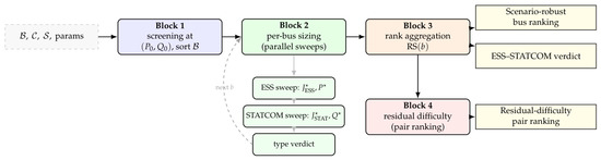
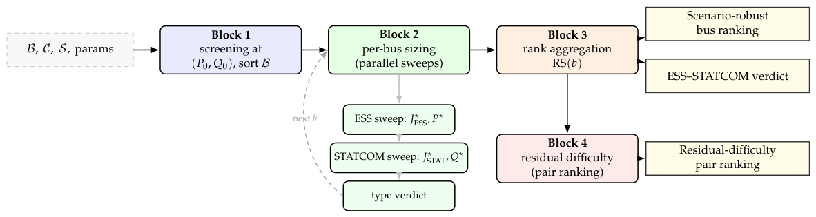
Figure 1. Workflow diagram of the proposed scenario-robust siting and ranking framework, the algorithmic counterpart of Problem (4). Block 1 performs screening at the reference capacity $(P_0,Q_0)$ and sorts $\mathcal{B}$. Block 2 executes per-bus sizing through two logically independent one-dimensional capacity sweeps (the ESS sweep on P and the STATCOM sweep on Q, which share no state or decision variable and may be evaluated in any order or in parallel) and assigns the ESS-better, STATCOM-better, or neutral verdict (the inner dashed arrow iterates over $b\in \mathcal{B}$). Block 3 aggregates the per-bus ranks into $\mathrm{RS}\left(b\right)$. Block 4 re-scores the N-2 pairs after optimal corrective support and ranks them by residual difficulty. The three planning outputs are the scenario-robust bus ranking, the per-bus ESS–STATCOM verdict, and the residual-difficulty pair ranking.

The scope of this paper is deliberately bounded to the screening, evaluation, and ranking layer of the corrective-support problem. It establishes a static post-contingency scoring rule, a scenario-robust rank-aggregation of candidate buses, and an explicit ESS-versus-STATCOM comparison under a transparent economic-weight ratio, and it isolates the contingencies that no single-node injection can resolve. It does not attempt a formal joint investment optimization. Capacity here is sized by per-resource one-dimensional sweeps rather than by a cost-minimizing program, and demand-side resources are outside its scope. Embedding the screening and ranking results developed here into a formal multi-resource investment-optimization model—one that jointly sizes ESS, STATCOM, and demand-side response under an explicit cost objective—is a substantial and distinct problem, identified as the principal direction of follow-up work (Section 6).

The remainder of this paper is organized as follows. Section 2 describes the study system, Section 3 presents the proposed framework, Section 4 reports the numerical results, Section 5 discusses their implications, and Section 6 concludes this paper.

2. Study System and Problem Setting

This section describes the study system, the contingency construction process, and the static post-contingency evaluation setting.

2.1. Security Implications of 765 kV Double-Circuit N-2 Contingencies

Power system security is described using the N-k criterion, where N-2 denotes the simultaneous loss of two facilities. The 765 kV network transfers substantially larger power than lower-voltage transmission systems [1]. When two parallel circuits within the same corridor are lost, power-flow redistribution is highly abrupt. Overloads concentrate on alternative facilities, and receiving areas become vulnerable to reactive-power deficiency and voltage depression [5,6].

The post-contingency state must satisfy both network equilibrium and static security constraints. Let $\mathcal{N}$ be the bus set and $\mathcal{L}$ be the line/transformer set. The AC power-balance equations under contingency c are

$$\begin{array}{cc}\hfill P_i& =\sum _{k\in \mathcal{N}}|V_i||V_k|\left[G_{ik}^{\left(c\right)}\cos \Delta {\theta }_{ik}+B_{ik}^{\left(c\right)}\sin \Delta {\theta }_{ik}\right],\hfill \end{array}$$

(1)

$$\begin{array}{cc}\hfill Q_i& =\sum _{k\in \mathcal{N}}|V_i||V_k|\left[G_{ik}^{\left(c\right)}\sin \Delta {\theta }_{ik}-B_{ik}^{\left(c\right)}\cos \Delta {\theta }_{ik}\right],i\in \mathcal{N},\hfill \end{array}$$

(2)

where $\Delta {\theta }_{ik}={\theta }_i-{\theta }_k$, and the static security constraints require

$$|S_{ij}|\le S_{ij}^{\max },(i,j)\in \mathcal{L};V_i^{\min }\le |V_i|\le V_i^{\max },i\in \mathcal{N}.$$

(3)

If no feasible post-contingency solution exists, or if the power flow fails to converge, the condition is interpreted as an insufficient steady-state security margin, the standard steady-state specialization of the general power system stability definition [16].

2.2. Key 765 kV Transmission Corridors and Candidate Buses

The 765 kV transmission system of the Republic of Korea links the east- and south-coast generation areas to the central load center and the western thermal-generation nodes. The 10 candidate buses are grouped by geographic role in Table 1. Throughout this paper individual substations of the Republic of Korea are anonymized to Bus A–Bus J so that the framework can be read without prior knowledge of the local substation names, and the geographic locations of these labels are summarized in the schematic map of Figure 2. The 500 kV HVDC Bus A–Bus E link is available from 2026 and is evaluated separately in both on/off states.

Table 1. Geographic grouping and principal roles of the ten 765 kV candidate buses in the Republic of Korea backbone. Individual substations are anonymized to Bus A–Bus J. The grouping in the first column is functional (by the role each substation plays in the bulk-transfer architecture), and it is not strictly geographic. In particular, Bus J is grouped here with Bus E as an east-coast nuclear receiving substation because both serve as 765 kV interfaces to large-scale nuclear output, even though Bus J is geographically located on the south-east coast and Bus E on the north-east coast, as reflected in Figure 2.

Geographic Role	Candidate Buses	Principal Role
East-coast nuclear corridor	Bus E, Bus J	Receiving substations for large-scale nuclear output
Inland backbone	Bus D, Bus F, Bus A	Main east-coast to metropolitan bulk-transfer chain
Central nodes	Bus C, Bus B	Aggregation and redistribution hubs for westbound power flow
West-coast generation nodes	Bus H, Bus G	Thermal-generation nodes serving western demand
Southern node	Bus I	Interface to the southern industrial load zone

Figure 2. Illustrative regional grouping of the ten 765 kV candidate buses in the Republic of Korea, together with the 765 kV double-circuit corridors that are evaluated as N-2 contingency pairs in the case data analyzed in this paper and an illustrative set of 345 kV inter-regional interconnections. Each shaded zone collects the buses that belong to a single geographic region of the country, in correspondence with the geographic role column of Table 1. Solid lines indicate the 765 kV double-circuit corridors enumerated in Table 2; the dashed line indicates the 500 kV HVDC link between Bus A and Bus E that is commissioned in 2026 and is included separately in the HVDC-on scenarios; the dashed-dotted lines indicate representative 345 kV inter-regional interconnections (Inland ↔ Central, Central ↔ West coast, Central ↔ Southern, and within-region links) that are present in the underlying case data but are not evaluated as part of the 765 kV double-circuit N-2 contingency set; they are shown only to indicate that the geographic regions are not topologically isolated at the sub-765 kV level. The figure is laid out by geographic region rather than to geographic scale, so the line lengths and angles do not correspond to physical distances. Substation names are anonymized to Bus A–Bus J as defined in Table 1.

Figure 2. Illustrative regional grouping of the ten 765 kV candidate buses in the Republic of Korea, together with the 765 kV double-circuit corridors that are evaluated as N-2 contingency pairs in the case data analyzed in this paper and an illustrative set of 345 kV inter-regional interconnections. Each shaded zone collects the buses that belong to a single geographic region of the country, in correspondence with the geographic role column of Table 1. Solid lines indicate the 765 kV double-circuit corridors enumerated in Table 2; the dashed line indicates the 500 kV HVDC link between Bus A and Bus E that is commissioned in 2026 and is included separately in the HVDC-on scenarios; the dashed-dotted lines indicate representative 345 kV inter-regional interconnections (Inland ↔ Central, Central ↔ West coast, Central ↔ Southern, and within-region links) that are present in the underlying case data but are not evaluated as part of the 765 kV double-circuit N-2 contingency set; they are shown only to indicate that the geographic regions are not topologically isolated at the sub-765 kV level. The figure is laid out by geographic region rather than to geographic scale, so the line lengths and angles do not correspond to physical distances. Substation names are anonymized to Bus A–Bus J as defined in Table 1.

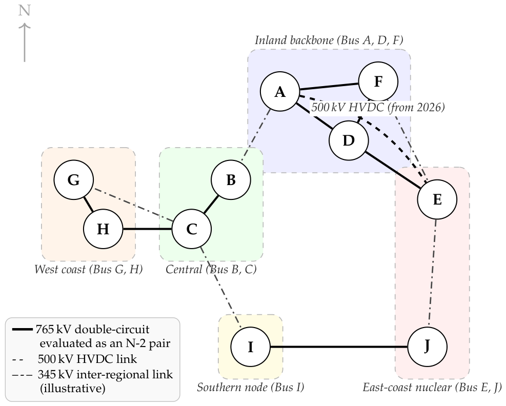
Table 2. Relative vulnerability comparison by N-2 contingency pair. The “Analyzed scen.” column counts only scenario files in which the pair survives coverage screening and yields a valid residual-difficulty entry, so it differs across pairs and may slightly exceed the 60 scenarios retained by the cost-ratio analysis (Section 4.6) because the residual-difficulty filter is per-pair rather than per-scenario. The “Worst-pair sel.” column counts the number of scenarios in which the pair is the single worst-ranked contingency after corrective support is optimally placed. Rows omitted from the table contribute the remainder, and tied worst pairs can sum to a count slightly larger than the number of scenarios. Pairs can additionally appear in Top-3 difficulty without being the worst.

N-2 Pair	Analyzed Scen.	Worst-Pair Sel.	Top-3 Diff. Entries	Avg. Rank
Bus A–Bus F	46	22	28	3.22
Bus I–Bus J	60	17	38	3.13
Bus A–Bus D	14	9	9	2.79
Bus D–Bus F	46	7	32	3.35
Bus D–Bus E	61	6	31	3.62
Bus C–Bus H	60	1	35	3.77
Bus G–Bus H	60	0	5	4.50
Bus B–Bus C	60	0	4	5.52

Table 2. Relative vulnerability comparison by N-2 contingency pair. The “Analyzed scen.” column counts only scenario files in which the pair survives coverage screening and yields a valid residual-difficulty entry, so it differs across pairs and may slightly exceed the 60 scenarios retained by the cost-ratio analysis (Section 4.6) because the residual-difficulty filter is per-pair rather than per-scenario. The “Worst-pair sel.” column counts the number of scenarios in which the pair is the single worst-ranked contingency after corrective support is optimally placed. Rows omitted from the table contribute the remainder, and tied worst pairs can sum to a count slightly larger than the number of scenarios. Pairs can additionally appear in Top-3 difficulty without being the worst.

N-2 Pair	Analyzed Scen.	Worst-Pair Sel.	Top-3 Diff. Entries	Avg. Rank
Bus A–Bus F	46	22	28	3.22
Bus I–Bus J	60	17	38	3.13
Bus A–Bus D	14	9	9	2.79
Bus D–Bus F	46	7	32	3.35
Bus D–Bus E	61	6	31	3.62
Bus C–Bus H	60	1	35	3.77
Bus G–Bus H	60	0	5	4.50
Bus B–Bus C	60	0	4	5.52

The east-coast inland backbone in Table 1 is the main bulk-transfer chain toward the metropolitan load center, the structural reason why outages involving Bus A, Bus D, and Bus F repeatedly emerge as high-severity pairs in the results.

2.3. Relationship Between ACCC and Static Post-Contingency Evaluation

The AC contingency calculation (ACCC) framework provides the conceptual basis for evaluating N-2 effects on the transmission network. A base operating point is solved, predefined contingencies are then sequentially applied, and the resulting power flow, voltage profile, and thermal-limit violations are repeatedly evaluated [9]. This repeated AC power-flow approach is consistent with multi-scenario stochastic power-flow evaluation frameworks used in transmission planning studies [17]. The conventional ACCC concept is extended here into a scenario-integrated corrective-support evaluation algorithm in which 765 kV double-circuit N-2 pairs are constructed automatically and the constraint alleviation achieved by ESS and STATCOM is evaluated per contingency [10].

The present study is confined to the static post-contingency regime. Every candidate is judged by post-contingency thermal-loading and voltage-security feasibility, and the framework is positioned as a pre-screening stage that narrows the 765 kV siting decision before any dynamic study is undertaken. Dynamic phenomena (transient stability, short-circuit strength, and frequency response) are out of scope by design. Surveys of dynamic security assessment document the substantial methodological gap between static screening and a full dynamic-security workflow [18], and these indicators are identified in Section 6 as the natural next stage.

2.4. Construction of N-2 Contingency Pairs and Candidate-Bus Set

This study automatically identifies 765 kV double-circuit line pairs and constructs the full N-2 pair set. Two lines form a valid pair only when they connect the same sending and receiving substations at 765 kV. Candidate buses are generated from the input bus data, deduplicated, and filtered to the 765 kV level.

2.5. System Data and Scenario Configuration

The system data reflect long-term network conditions based on the 6th (2013) and 7th (2015) Basic Plans for Long-term Electricity Supply and Demand of the Republic of Korea, reviewed against the 10th Basic Plan (2023). The dataset represents a multi-year planning perspective incorporating changes in demand, generation, operating conditions, and transmission configuration.

Table 3 summarizes the demand and generation assumptions. Peak load grows from 98.8 GW (2023) to 113.6 GW (2033), and medium and off-peak conditions are set to 80% and 60% of peak, respectively. Installed generation capacity grows from 116.8 GW to 139.9 GW, reflecting the increased renewable share and the 4.5 GW operating reserve of the 10th Basic Plan.

Table 3. Summary of demand and generation conditions.

Category	Condition	2023 (GW)	2026 (GW)	2033 (GW)
Demand	Peak	98.8	104.2	113.6
	Medium	79.0	83.4	90.9
	Off-peak	59.3	62.5	68.2
Generation	Installed capacity	116.8	129.6	139.9
	Peak output	101.6	107.2	119.5
	Medium output	82.2	86.6	97.9
	Off-peak output	61.2	65.0	72.9

Beyond the demand and generation figures in Table 3, the transmission configuration is differentiated by year. The 500 kV HVDC Bus A–Bus E line is assumed as in service from 2026 onward and is represented in the static AC power flow as a two-terminal scheduled-power link, with reactive-power contributions of the converter stations bounded by the per-station limits stored in the case file rather than introduced as additional decision variables of the framework. Under this representation the “HVDC-on” state imposes the scheduled link flow, the “HVDC-off” state disables the link, and dynamic converter controls are outside the scope of the static post-contingency evaluation. Accordingly, the 2026 and 2033 scenarios are analyzed under both HVDC-on and HVDC-off conditions, and the 2023 scenario is modeled without HVDC and serves as the pre-commissioning baseline:

• Year 2023: Pre-HVDC baseline case.
• Year 2026: 500 kV HVDC Bus A–Bus E line available.
• Year 2033: Long-term expanded system with the HVDC line retained.

2.6. Definition of the Scenario Set

The full scenario set combines four axes. Study year (2023, 2026, and 2033), load level (peak, medium, and off-peak), planning condition (6thPlan, 7thPlan, and No2nd), and HVDC operating state (on/off, where applicable). The three planning-condition labels denote the generation- and transmission-expansion inputs adopted in each case. The 6thPlan label follows the 6th Basic Plan (2013) for Long-term Electricity Supply and Demand, 7thPlan adopts the updated generation and corridor assumptions of the 7th Basic Plan (2015), and No2nd retains the 7th Basic Plan (2015) generation set but excludes the second-circuit reinforcement of the inland backbone that the 7th Plan added. A candidate bus that performs strongly under one year or load level is not automatically robust under the full scenario set. The scenario structure therefore transforms the siting problem from a single-case engineering decision into a multi-scenario planning decision, analogous in spirit to long-term transmission expansion planning studies that must accommodate structural uncertainty [7].

3. Scenario-Robust Siting and Ranking Framework

Before describing the algorithmic components, the underlying selection problem is stated in compact form. Let $\mathcal{B}$ denote the set of admissible 765 kV candidate buses (Section 2.2), let $\mathcal{C}$ denote the set of 765 kV double-circuit N-2 contingencies (Section 2.4), and let $\mathcal{S}$ denote the multi-scenario set spanning study year, load level, planning condition, and HVDC state (Section 2.6). For each candidate $(b,P,Q)\in \mathcal{B}\times [0,P_{\max }]\times [0,Q_{\max }]$ and each scenario $s\in \mathcal{S}$, let $S_s^{\left(c\right)}(b,P,Q)$ denote the post-contingency score (Definition 1) under contingency $c\in \mathcal{C}$. The scenario-robust siting and ranking problem is then

$$\left(\mathrm{P}\right)\underset{b\in \mathcal{B}}{\min }\mathrm{RS}\left(b;\overline{S},\overline{I},\mathrm{Rel}\right)\mathrm{s}.\mathrm{t}.\left\{\begin{array}{c}\overline{S}(b,P,Q)=\frac{1}{|\mathcal{S}||\mathcal{C}|}{\displaystyle \sum _{s,c}}{S}_s^{\left(c\right)}(b,P,Q),\hfill \\ P\in \arg {\min }_{P^{\prime }}{J}_{\mathrm{ESS}}(b,P^{\prime }),\hfill \\ Q\in \arg {\min }_{Q^{\prime }}{J}_{\mathrm{STAT}}(b,Q^{\prime }),\hfill \\ \mathrm{feasibility}:\mathrm{no}\mathrm{islanding},\mathrm{no}\mathrm{divergence},\hfill \end{array}\right.$$

(4)

where $\mathrm{RS}(·)$ is the scenario-robust score of Definition 3, the inner $\arg \min$ problems are the per-axis capacity sweeps of Section 3.7, and the feasibility constraint requires a converged post-contingency operating point for at least the minimum required fraction of sub-scenarios. Problem (4) is treated by decomposition. The inner sizing problems are handled by independent one-dimensional sweeps with finite termination guaranteed by Theorem 1, while the outer ranking objective is evaluated off-line after all per-scenario AC power flows have been solved. The framework comprises three interacting layers, namely an optimal-location layer that proposes candidate 765 kV buses and sizes ESS/STATCOM support at each candidate, a robustness layer that aggregates per-contingency severity across the multi-scenario set, and a ranking layer that converts the aggregate into $\mathrm{RS}\left(k\right)$ and the residual-difficulty signal. The remaining subsections develop each layer in turn.

3.1. Physical Roles of ESS and STATCOM in the Post-Contingency Regime

ESS operates through active-power injection or absorption and directly modifies post-contingency power-transfer paths, reducing thermal congestion on heavily loaded lines [11,13]. This controllable active-power capability makes ESS a dispatchable corrective resource at the transmission level. STATCOM primarily provides reactive-power support and therefore mitigates voltage depression and improves voltage-security margins [15]. Its principal contribution in the post-contingency state is to prevent voltage collapse in receiving-area buses that lose reactive-power support when a 765 kV double-circuit is lost. A grid-connected battery is interfaced through a four-quadrant converter and can in principle supply reactive power alongside active power, so the ESS–STATCOM distinction is one of energy buffering rather than of reactive capability [19]; the framework nonetheless decouples the two—assigning active support to the ESS branch and reactive support to the STATCOM branch—to return an interpretable per-bus verdict, and a combined active–reactive device would approach an integrated hybrid ESS–STATCOM whose joint two-dimensional $(P,Q)$ sizing is a direct generalization.

The relative effectiveness of the two resources depends on the dominant type of post-contingency violation. ESS is more effective when the primary limitation is thermal congestion driven by active-power redistribution, whereas STATCOM provides stronger benefit when voltage weakness is dominant. Accordingly, the two resources are treated as complementary rather than substitutable throughout this study.

3.2. Congestion-Relief and Voltage-Support Mechanisms

Building on Section 3.1, the effect of each resource is evaluated by solving the post-contingency AC flow after applying injection P (ESS) or Q (STATCOM) at bus b. Active-power injection alters branch flows and mainly addresses overloads, while reactive-power injection alters local voltage magnitudes and mainly addresses voltage-security violations. The overall post-contingency severity is summarized by the weighted penalty index

$${\Phi }^{\left(c\right)}=w_V{\varphi }^V+w_O{\varphi }^O+w_D{\varphi }^D+w_S{\varphi }^S+w_I{n}_I+w_M{\varphi }^M,$$

(5)

where ${\varphi }^V={\sum }_{i\in \mathcal{N}}\left[\max (V^{\min }-|V_i|,0)+\max (|V_i|-V^{\max },0)\right]$ is the total bus voltage-limit violation, ${\varphi }^O={\sum }_{\ell \in \mathcal{L}}\max ({\mathrm{load}}_{\ell }-100\%,0)$ is the total thermal overload beyond rating, ${\varphi }^D={\sum }_{i\in \mathcal{N}}\left||V_i|-1\right|$ is the total voltage deviation from nominal, ${\varphi }^S$ is the swing-bus active/reactive limit violation, $n_I$ is the number of islanded buses, and ${\varphi }^M$ is the total bus MVA mismatch. All violation terms are linear (first-order) sums, so no single term dominates purely through quadratic scaling. A larger ${\Phi }^{\left(c\right)}$ indicates a more severe post-contingency state and explains why certain N-2 pairs repeatedly emerge as dominant difficult cases. This severity index is the post-contingency score $S^{\left(c\right)}$ used in the candidate evaluation defined in the following subsection.

3.3. Post-Contingency Score $S^{\left(c\right)}$

The per-contingency score consumed by the ranking pipeline is exactly the weighted linear penalty index ${\Phi }^{\left(c\right)}$ introduced in Section 3.2. This weighted-penalty construction follows the established performance-index methodology for contingency ranking [20]; the six weights encode a three-tier engineering-severity ordering (operating-point-invalidating conditions are highest, genuine security-limit excursions are in the middle, and mild local excursions are at the base), so that only the tier separation, not the exact numerical values, is intended to matter. A sensitivity analysis on these weights is provided in Appendix Table A2 and confirms that the ranking is preserved under every tier-preserving perturbation and changes only when the hierarchy is inverted.

Definition 1

(Post-contingency score). For a candidate bus b with active-power injection P and reactive-power injection Q, and an N-2 contingency $c\in \mathcal{C}$, the post-contingency score $S^{\left(c\right)}(b,P,Q)$ is the weighted linear penalty index ${\Phi }^{\left(c\right)}$ of Equation (5) evaluated on the solved post-contingency operating point obtained after applying the injection $(P,Q)$ at bus b and tripping the two circuits of contingency c. If the AC power flow fails to converge or yields no valid operating point, $S^{\left(c\right)}(b,P,Q)$ is set to the fixed non-convergence penalty M.

The fixed weights are $(w_V,w_O,w_D,w_S,w_I,w_M)=(1,5,5,1,50,10)$ and $M={10}^3$. The voltage band $[V^{\min },V^{\max }]=[0.95,1.05]$ pu follows the conservative range of the Korean reliability and electricity-quality standard [21], and the overload term uses a $100\%$ thermal-rating threshold. The weights are ordered by engineering severity rather than tuned. Violations that invalidate the operating point dominate (islanding $w_I=50$; mismatch $w_M=10$), overload and aggregate voltage deviation form the middle tier ($w_O=w_D=5$), and pointwise voltage-limit and swing-limit violations form the base tier ($w_V=w_S=1$). This ordinal ordering is preserved under any positive monotone rescaling, so the ranking is insensitive to the precise values as long as the tiers stay disjoint. A formal rank-aggregation weight-sensitivity analysis appears in Section 4.4.

3.4. Candidate Evaluation and Economic Comparison Metric

Each candidate is evaluated by repeated post-contingency AC power flow over the scenario set of Section 2.6. For a candidate bus b with support capacity $(P,Q)$, the scenario-averaged quantities consumed by the pipeline are defined as follows.

Definition 2

(Scenario-averaged score and improvement). For a candidate $(b,P,Q)$ evaluated over the scenario set $\mathcal{S}$ (Section 2.6) and the N-2 contingency set $\mathcal{C}$ (Section 2.4), the scenario-averaged score and scenario-averaged improvement are

$$\begin{array}{cc}\hfill \overline{S}(b,P,Q)& ={\displaystyle \frac{1}{|\mathcal{S}||\mathcal{C}|}}\sum _{s\in \mathcal{S}}\sum _{c\in \mathcal{C}}{S}_s^{\left(c\right)}(b,P,Q),\hfill \end{array}$$

(6)

$$\begin{array}{cc}\hfill \overline{I}(b,P,Q)& ={\displaystyle \frac{1}{|\mathcal{S}||\mathcal{C}|}}\sum _{s\in \mathcal{S}}\sum _{c\in \mathcal{C}}\left[S_{0,s}^{\left(c\right)}-S_s^{\left(c\right)}(b,P,Q)\right],\hfill \end{array}$$

(7)

where $S_s^{\left(c\right)}$ is the post-contingency score of Definition 1 in scenario s, and $S_{0,s}^{\left(c\right)}$ is the corresponding no-support baseline. Evaluations that fail to converge are counted as failures and excluded from $\overline{S},\overline{I}$ but retained in the reliability statistic used in Section 3.8.

Candidate evaluation proceeds in two stages. In the screening stage, every candidate bus is evaluated once at a fixed reference capacity $(P_0,Q_0)=(500\mathrm{MW},150\mathrm{Mvar})$, and the buses are ordered by their screening score. In the sizing stage, ESS and STATCOM are sized independently. An ESS branch sweeps active power P with $Q=0$, a STATCOM branch sweeps reactive power Q with $P=0$, and each sweep is scored by a capacity-penalized metric

$$J_{\mathrm{ESS}}(b,P)=\overline{S}(b,P,0)+{\gamma }_{\mathrm{ESS}}|P|,J_{\mathrm{STAT}}(b,Q)=\overline{S}(b,0,Q)+{\gamma }_{\mathrm{STAT}}|Q|,$$

(8)

where $({\gamma }_{\mathrm{ESS}},{\gamma }_{\mathrm{STAT}})$ are economic weights fixed at the ratio ${\gamma }_{\mathrm{ESS}}:{\gamma }_{\mathrm{STAT}}=3:1$. This ratio is a normalized planning proxy anchored to public utility-scale battery-storage cost benchmarks and to the lower per-MVAr investment burden of shunt reactive-power compensation equipment [22,23]. To avoid treating the proxy as fixed economic truth, Section 4.5 reports the neutral cases and explicitly discusses sensitivity to this assumed ratio.

For each candidate bus, the best feasible ESS size minimizes $J_{\mathrm{ESS}}$, and the best feasible STATCOM size minimizes $J_{\mathrm{STAT}}$. A capacity is admitted only if it yields a feasible post-contingency operating point (no islanding, no divergence, and no failed sub-scenario). The bus is then labeled ESS-better, STATCOM-better, or neutral according to which capacity-penalized metric is smaller, with a tolerance band defining the neutral (no-decision) outcome. Because feasibility is enforced inside each sweep, infeasible capacities never compete with feasible ones, so the comparison is feasible-first by construction.

3.5. Implementation Settings

Table 4 summarizes the main algorithm settings, fixed throughout this study so that cross-scenario comparisons reflect structural differences rather than parameter sensitivity. The screening reference capacity is of the order of one utility-scale battery block and one transmission-class STATCOM rating; it affects only the order in which buses enter the sizing stage, since every bus is subsequently re-sized over the full sweep, so the final ranking is set by the swept optima rather than by the reference capacity. All post-contingency AC power flows are computed in Siemens PSS^®E 34 through its Python 2.7 API, with Newton–Raphson iteration and the engine’s standard convergence flags applied identically across all cases.

Table 4. Main algorithm settings used throughout this study.

Item	Value	Description
Target voltage	765 kV	Only 765 kV lines are used to construct valid double-circuit N-2 pairs.
Valid N-2 pair	Same bus pair, 2 circuits	Two lines form a valid pair only when they belong to the same 765 kV double-circuit corridor.
Candidate filter	765 kV buses	Candidate siting buses are taken at the 765 kV level (renewable-injection buses excluded).
Screening capacity	$P_0=500$ MW, $Q_0=150$ Mvar	Fixed reference capacity applied to every candidate bus in the screening stage.
Sizing-stage buses	All screened buses	Every screened bus is sized, and buses are processed in descending screening-score order.
Capacity sweep range	ESS up to 4000 MW and STATCOM up to 4000 Mvar	Per-axis defense limit applied independently to the ESS active-power sweep and the STATCOM reactive-power sweep.
Sweep step sizes	ESS 100 MW, STATCOM 10 Mvar	Linear capacity increments for the independent ESS (P) and STATCOM (Q) sweeps.
Sweep termination	2 steps without improvement	Each sweep stops after two consecutive increments fail to improve the capacity-penalized metric beyond a $0.1$ tolerance.
Zero-capacity anchor	$(0,0)$ included	The no-installation case is the sweep starting point and reference.
Economic weights	ESS : STATCOM $=3:1$	Capacity-penalty ratio in the ESS/STATCOM comparison metric, Equation (8).
Failure treatment	No-result	Solver failure or non-convergence is recorded and excluded from the robust ranking.
Robust-score weights	0.65/0.25/0.10	Weights assigned to score rank, improvement rank, and reliability, respectively.

The screening capacity $(P_0,Q_0)=(500\mathrm{MW},150\mathrm{Mvar})$ discriminates candidate buses without masking individual characteristics. The capacity sweeps extend up to a 4000-unit defense limit (MW for ESS; Mvar for STATCOM), far above any realistic single-site installation, so the sweep range itself acts as an extreme test. If neither sweep restores feasibility even at this near-unlimited capacity, the contingency is identified as structurally unsolvable by single-node compensation, as reported jointly in Section 4.6. All settings are applied identically across scenarios.

3.6. Overall Workflow

The end-to-end procedure is given as Figure 1. The target system case is loaded, all 765 kV double-circuit line pairs are automatically identified, candidate buses are screened under the fixed reference capacity $(P_0,Q_0)$, each screened bus is sized along independent ESS and STATCOM capacity sweeps, and feasible solutions are prioritized in the final scenario-robust ranking. The hierarchy keeps the per-scenario cost bounded by Corollary 1 and records solver non-convergence as part of the reliability outcome rather than discarding it silently.

Each step of Figure 1 corresponds to a self-contained function described in Appendix A, so the same workflow can be re-executed with a different case file or scenario list without modifying intermediate stages.

3.7. Hierarchical Screening and Independent Capacity Sizing

In the screening stage, every candidate bus is evaluated once at $(P_0,Q_0)=(500\mathrm{MW},$ $150\mathrm{Mvar})$ and ordered by screening score. In the sizing stage, each bus is sized by two independent 1D sweeps. The ESS branch sweeps P in 100 MW steps with $Q=0$, and the STATCOM branch sweeps Q in 10 Mvar steps with $P=0$, each up to 4000 MW or 4000 Mvar. An increment is retained only if the resulting operating point is feasible (no islanding, no divergence, and no failed sub-scenario) and improves the capacity-penalized metric of Equation (8) by more than $0.1$, and the sweep stops after two consecutive non-improving increments [24]. The best feasible ESS and STATCOM sizes are then compared through their capacity-penalized metrics, and the bus is labeled ESS-better, STATCOM-better, or neutral.

Two design choices keep the sizing tractable. First, screening supplies a structurally informed processing order so effective buses are sized first. Second, sweeping ESS and STATCOM separately avoids the 2D search, with the active- and reactive-power axes sized independently and compared afterwards. Calculation failures and non-convergence are no-result [25], and a bus that neither a modest ESS nor a modest STATCOM restores to feasibility is flagged as a defense failure. A candidate that cannot restore feasibility within the 4000-unit limit for a contingency is marked structurally unsolvable and excluded from that candidate’s scenario-averaged score.

The complete framework is summarized as a workflow diagram in Figure 1, which serves as the algorithmic counterpart of Problem (4). The pipeline takes the candidate-bus set $\mathcal{B}$, the N-2 pair set $\mathcal{C}$, the scenario set $\mathcal{S}$, and the algorithm parameters $(P_0,Q_0,C_{\max },{\Delta }_{\mathrm{ESS}},{\Delta }_{\mathrm{STAT}},\tau ,{\gamma }_{\mathrm{ESS}},{\gamma }_{\mathrm{STAT}},{\omega }_{\mathrm{score}},{\omega }_{\mathrm{imp}},{\omega }_{\mathrm{rel}})$ as input and proceeds in four blocks. Block 1 (screening) evaluates every candidate once at the reference capacity $(P_0,Q_0)$ over $\mathcal{S}\times \mathcal{C}$ and sorts $\mathcal{B}$ by screening score. Block 2 (per-bus sizing) executes the ESS sweep on P with step ${\Delta }_{\mathrm{ESS}}$ and the STATCOM sweep on Q with step ${\Delta }_{\mathrm{STAT}}$ in parallel for each $b\in \mathcal{B}$, each retaining a step only when it is feasible and improves the capacity-penalized metric of Equation (8) by more than $\tau$, terminating after two consecutive non-improving steps (Theorem 1) and then assigning the ESS-better, STATCOM-better, or neutral verdict by comparing the two capacity-penalized optima. Block 3 (rank aggregation) computes the normalized score and improvement ranks together with the reliability and evaluates $\mathrm{RS}\left(b\right)$ by Definition 3. Block 4 (residual-difficulty layer) re-scores each N-2 pair with corrective support placed at the scenario-level winner and ranks pairs by their residual difficulty. The three outputs are the scenario-robust bus ranking, the per-bus type verdict, and the residual-difficulty pair ranking.

3.8. Statistical Re-Scoring Algorithm

In the post-processing stage, an integrated robust score is computed for each surviving candidate. The three rank-aggregation weights are set by a transparent ordinal rule in the spirit of ordered-weighted-averaging operators [26]—the largest weight on score rank, the next on improvement rank, and the smallest on reliability as a tie-breaker—so the specific triple $(0.65,0.25,0.10)$ is one ordinal assignment rather than a fitted value.

Definition 3

(Scenario-robust score). Let $R_{\mathrm{score}}\left(k\right)\in [0,1]$ and $R_{\mathrm{imp}}\left(k\right)\in [0,1]$ denote the normalized score and improvement ranks of candidate k, and let $\mathrm{Rel}\left(k\right)\in [0,1]$ denote the empirical success rate of its evaluations. The scenario-robust score is

$$\begin{array}{cc}\hfill \mathrm{RS}\left(k\right)\equiv & 100({\omega }_{\mathrm{score}}{R}_{\mathrm{score}}\left(k\right)+{\omega }_{\mathrm{imp}}{R}_{\mathrm{imp}}\left(k\right)\hfill \\ \hfill & +{\omega }_{\mathrm{rel}}[1-\mathrm{Rel}\left(k\right)]),\hfill \end{array}$$

(9)

with rank-aggregation weights $({\omega }_{\mathrm{score}},{\omega }_{\mathrm{imp}},{\omega }_{\mathrm{rel}})$ satisfying ${\omega }_{•}\ge 0$ and ${\sum }_{•}{\omega }_{•}=1$, and with lower $\mathrm{RS}\left(k\right)$ preferred. The default configuration used throughout is $({\omega }_{\mathrm{score}},{\omega }_{\mathrm{imp}},{\omega }_{\mathrm{rel}})=(0.65,0.25,0.10)$. These rank-aggregation weights are distinct from the economic weights ${\gamma }_{\mathrm{ESS}},{\gamma }_{\mathrm{STAT}}$ in Equation (8).

The default weights are chosen by a transparent ordinal rule rather than by external tuning, in the spirit of ordered-weighted aggregation operators [26]. The largest weight is placed on score rank as the primary planning objective, the next is placed on improvement rank to separate candidates with similar absolute scores, and the smallest is placed on reliability as a tie-breaker because failures are already flagged before re-scoring. Ties at the integer-rank level are broken first by the raw score $\overline{S}(b,P,Q)$ and then by the raw improvement $\overline{I}(b,P,Q)$, so that the rank-aggregation is well-defined even when several candidates share an integer rank. The metric is scenario-averaged rank-robust rather than worst-case robust in the min–max sense of classical robust optimization [27]. The appropriate worst-case extension would replace the scenario average $\overline{S}$ in $R_{\mathrm{score}}$ by ${\max }_{c\in \mathcal{C}}{S}^{\left(c\right)}$, while a complementary direction is a distributionally robust optimization that hedges against an ambiguity set of scenario distributions [28]. Both extensions are left to future work. Sensitivity to the weight choice is quantified in Section 4.4. Rows with failures, within-tolerance ties (band of ${10}^{-3}$ on the capacity-penalized metric of Equation (8)), or fewer than the minimum required valid cases are excluded. The framework yields three complementary outputs, namely a pair-level ranking, a scenario-level robust ranking, and a vulnerable-pair ranking from residual difficulty after optimal support placement.

Theorem 1

(Finite termination of the capacity sweep). For each candidate bus b and each support type (ESS active-power sweep; STATCOM reactive-power sweep), the capacity sweep of Section 3.7 terminates in at most $\lceil C_{\max }/\Delta \rceil +2$ evaluations, where $C_{\max }=4000$ is the upper capacity bound, and $\Delta \in \{100\mathrm{MW},10\mathrm{Mvar}\}$ is the per-axis step size, regardless of the post-contingency score values returned by the AC power-flow engine.

Proof. 

Each sweep starts at zero and advances by one step $\Delta$ per iteration, so the capacity reaches $C_{\max }$ in at most $\lceil C_{\max }/\Delta \rceil$ iterations. The early-stopping rule terminates after at most 2 additional non-improving iterations, giving a bound of $\lceil C_{\max }/\Delta \rceil +2$ that is independent of the score sequence. With $C_{\max }=4000$, the ESS sweep ($\Delta =100$ MW) takes at most 42 evaluations, and the STATCOM sweep ($\Delta =10$ Mvar) takes at most 402 per (bus, contingency, and scenario). □

This finite-termination property is what makes the overnight batch in Section 3.5 possible. The total number of AC power-flow solves per scenario is bounded a priori by Theorem 1 multiplied by the candidate-bus and N-2 pair counts, so the wall-clock budget can be planned without relying on solver-dependent stopping behavior. Theorem 1 immediately yields a global complexity bound for Problem (4).

Corollary 1

(Total complexity of Problem (4)). The total number of AC power-flow solves required by Figure 1 to compute the scenario-robust ranking ${\left\{\mathrm{RS}\left(b\right)\right\}}_{b\in \mathcal{B}}$ is bounded by

$$N_{\mathrm{solve}}\le |\mathcal{S}||\mathcal{C}||\mathcal{B}|\left(1+⌈C_{\max }/{\Delta }_{\mathrm{ESS}}⌉+⌈C_{\max }/{\Delta }_{\mathrm{STAT}}⌉+4\right),$$

where the first 1 accounts for the screening evaluation, and the $+4$ absorbs the two early-stopping tails of Theorem 1.

Proof. 

For each scenario $s\in \mathcal{S}$, each contingency $c\in \mathcal{C}$, and each candidate $b\in \mathcal{B}$, the algorithm performs one screening AC solve plus the two independent sweeps. By Theorem 1, each sweep performs at most $\lceil C_{\max }/\Delta \rceil +2$ AC solves. Summing the two sweeps and the screening solve gives the per-triple bound, and multiplying by $|\mathcal{S}||\mathcal{C}||\mathcal{B}|$ gives the stated total. □

3.9. Theoretical Properties

Beyond finite termination, three additional properties make Problem (4) well-posed and tractable. Practically, finite termination and the complexity bound fix the number of solves in advance, existence guarantees a well-defined size per candidate, the exact decomposition makes the per-bus sizing parallelizable, and bootstrap consistency lets the reported intervals be read as honest uncertainty statements.

Proposition 1

(Existence of an optimal sized capacity). For every candidate $b\in \mathcal{B}$ whose no-support baseline score $\overline{S}(b,0,0)$ is finite, the capacity-penalized ESS metric $J_{\mathrm{ESS}}(b,P)=\overline{S}(b,P,0)+{\gamma }_{\mathrm{ESS}}|P|$ is bounded below by ${\gamma }_{\mathrm{ESS}}|P|\ge 0$ and attains its minimum on the finite sweep grid $\{0,{\Delta }_{\mathrm{ESS}},2{\Delta }_{\mathrm{ESS}},\dots ,\lceil C_{\max }/{\Delta }_{\mathrm{ESS}}\rceil {\Delta }_{\mathrm{ESS}}\}$ restricted to feasible operating points. The analogous statement holds for $J_{\mathrm{STAT}}(b,Q)$.

Proof. 

$J_{\mathrm{ESS}}$ is the sum of two non-negative terms, and the feasibility-filtered sweep grid is non-empty (since $P=0$ is feasible by assumption), so a real-valued function on a non-empty finite set attains its minimum. The same argument applies to $J_{\mathrm{STAT}}$. □

Proposition 2

(Decomposition of Problem (4)). Under the capacity-penalized metric of Equation (8) and the rank-aggregation score of Definition 3, Problem (4) decomposes into $|\mathcal{B}|$ independent inner sizing problems

$$P^{\star }\left(b\right)\in \arg \underset{P\in [0,C_{\max }]}{\min }{J}_{\mathrm{ESS}}(b,P),Q^{\star }\left(b\right)\in \arg \underset{Q\in [0,C_{\max }]}{\min }{J}_{\mathrm{STAT}}(b,Q),$$

followed by a single outer ranking step that evaluates $\mathrm{RS}\left(b\right)$ on ${\left\{(b,P^{\star }\left(b\right),Q^{\star }\left(b\right))\right\}}_{b\in \mathcal{B}}$. The decomposition is exact whenever the rank-aggregation weights of Definition 3 are bus-independent.

Proof. 

$J_{\mathrm{ESS}}(b,P)$ and $J_{\mathrm{STAT}}(b,Q)$ depend on b only and not on any other bus, so the inner optima $P^{\star }\left(b\right)$ and $Q^{\star }\left(b\right)$ can be obtained per bus independently. Once the inner solutions are fixed, $\mathrm{RS}\left(b\right)$ depends only on per-bus quantities and the bus-independent weights $({\omega }_{\mathrm{score}},{\omega }_{\mathrm{imp}},{\omega }_{\mathrm{rel}})$, so the outer ranking is an exact aggregation of the inner solutions. □

Proposition 3

(Consistency of the percentile-bootstrap confidence intervals). Let ${\widehat{p}}_b$ denote the empirical top-share of bus $b\in \mathcal{B}$ over $|\mathcal{S}|$ independent scenarios, and let ${\widehat{p}}_b^{(*1)},\dots ,{\widehat{p}}_b^{(*B)}$ denote the percentile-bootstrap replicates obtained by resampling scenarios independently with replacement. Then, as $B\to \infty$ with $|\mathcal{S}|$ fixed, the $1-\alpha$ percentile-bootstrap confidence interval $[{\widehat{p}}_b^{*(\alpha /2)},{\widehat{p}}_b^{*(1-\alpha /2)}]$ converges in probability to a fixed deterministic interval, and, as $|\mathcal{S}|\to \infty$, this interval has asymptotic coverage equal to the nominal level $1-\alpha$.

Proof. 

The first convergence follows from the law of large numbers applied to the empirical quantile of the bootstrap distribution. The second is the classical first-order consistency of the percentile bootstrap for empirical averages with finite variance [29], applied here to the bounded scenario-level indicator of bus b being top-ranked. □

Proposition 1 guarantees that the inner sizing problems are well-posed. Proposition 2 justifies the decomposition that turns a high-dimensional joint problem into $|\mathcal{B}|$ independent low-dimensional searches, and Proposition 3 legitimizes the percentile-bootstrap confidence intervals used throughout the results.

4. Results

Three ranking outputs are reported, namely pair-level best-bus selection, scenario-level robust ranking, and the corridor-vulnerability signal. Case labels reflect year (2023, 2026, and 2033), load level (peak, medium, and off-peak), planning condition (6thPlan, 7thPlan, and No2nd, defined in Section 2.6), and HVDC state (on/off). The ten candidate buses carry the anonymized labels Bus A–Bus J defined in Table 1.

4.1. Pair-Level and Scenario-Level Candidate Rankings

Throughout the figures and the discussion that follows, the ten candidate buses are labeled Bus A–Bus J. The anonymized label and the internal bus code are listed in the first two columns of Table 5 so that the figure label and the headline percentages can be read together at a single location, while the geographic role of each bus is fixed in Table 1.

Table 5. Top-ranked shares by anonymized candidate bus (Bus A–Bus J), internal bus code, and percentile-bootstrap 95% confidence intervals [29] with $B=2000$ scenario-level resamples.

Bus Label	Bus Code	Pair-Level (%)	Pair 95% CI	Scenario-Level (%)	Scenario 95% CI
Bus A	1020	12.0	[9.2, 15.0]	7.7	[1.5, 15.4]
Bus B	4010	15.0	[11.5, 18.5]	4.6	[0.0, 10.8]
Bus C	4020	48.6	[43.7, 53.1]	13.9	[6.2, 23.1]
Bus D	5010	6.6	[4.2, 9.2]	32.3	[21.5, 43.1]
Bus E	5020	13.2	[10.1, 16.4]	6.2	[1.5, 12.3]
Bus F	5040	3.1	[1.6, 4.7]	16.9	[7.7, 26.2]
Bus G	6020	0.2	[0.0, 0.7]	6.2	[1.5, 12.3]
Bus H	6030	0.2	[0.0, 0.7]	4.6	[0.0, 10.8]
Bus I	8010	0.2	[0.0, 0.7]	0.0	[0.0, 0.0]
Bus J	9010	0.9	[0.2, 1.9]	7.7	[1.5, 15.4]

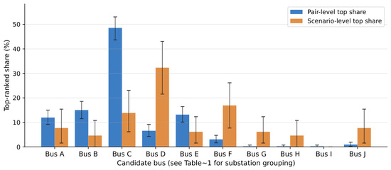
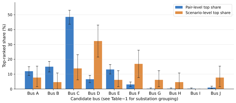
Table 5 summarizes the central ranking result. At the pair-level, Bus C is selected most frequently, accounting for 198 of 407 N-2 pairs (48.6%). At the scenario-level, however, Bus D becomes the leading candidate with a 32.3% top-ranked share, followed by Bus F at 16.9% and Bus C at 13.9%. The two rankings therefore identify different preferred buses, confirming that a siting decision based on a single severe outage pair does not generalize to the broader scenario space.

The contrast between the third and fifth numerical columns of Table 5 is best read jointly with the bar chart of Figure 3, which shows the pair-level and scenario-level shares side by side for every candidate. The bar-chart view also makes the asymmetry of the bootstrap 95% confidence intervals visible at a glance, in particular for the buses with very small pair-level share, where the upper CI bound dominates over the point estimate.

Figure 3. Pair-level (blue) versus scenario-level (orange) top-ranked share for each candidate bus, with bootstrap 95% confidence intervals shown as error bars (B = 2000 resamples).

Figure 3 confirms the divergence at the level of the individual buses. The scenario-level top-3 are statistically separated from the lower group, motivating the more detailed year/load/HVDC decomposition presented next.

4.2. Scenario-Level Sensitivity Summary

This subsection aggregates the sensitivity signal across the year, load, planning, and HVDC axes. The scenario-level sensitivity across the full scenario axes is summarized in Table 6. The 2023 cases remain relatively concentrated, whereas the 2026 and 2033 cases exhibit broader dispersion under medium- and peak-load conditions. HVDC has limited influence on the pair-level dominant bus but a clearer effect on the scenario-level robust ranking. Among 16 matched HVDC on/off scenario pairs, the final top-ranked candidate changes in 10 cases (62.5%).

Table 6. Scenario-level sensitivity summary across year, load, planning, and HVDC axes.

Axis	Representative Result	Implication
2023	Medium-load cases center on Bus C, and off-peak cases on Bus A.	Candidate concentration is clear in the pre-HVDC baseline system.
2026	Medium and peak cases are shared among Bus D, Bus F, Bus C, and Bus J.	HVDC commissioning and expanded generation reorder the robust ranking.
2033	Off-peak cases favor Bus D, and medium and peak cases remain dispersed.	Long-term structural change broadens the effective mitigation region.
HVDC	Pair-level top remains Bus C, but 10/16 matched on/off scenarios change the scenario-level winner.	HVDC affects the robust ranking more strongly than it affects pair-level local optima.

Table 6 reinforces the previous observations. The robust winner is far more sensitive to scenario axes than the pair-level dominant bus. This motivates a separate corridor-level view of residual difficulty, which is examined in the following subsection.

4.3. Vulnerable N-2 Pair Ranking

Table 2 summarizes residual corridor difficulty. The most frequent representative worst pair is Bus A–Bus F, whereas Bus I–Bus J records the largest number of Top-3 difficulty entries. These two pairs represent different threat profiles. The former is the most characteristic worst-pair contingency, while the latter remains persistently difficult across a broader portion of the scenario set. Representative post-contingency power-flow results for selected cases, showing which contingencies cause thermal and voltage violations, are provided in Appendix Table A1, and the specific N-2 pairs that drive each top-ranked bus are tabulated in Appendix Table A4.

The worst-pair analysis in Table 2 also reveals an important sub-finding. The locally preferred candidate for the most severe contingencies differs from the globally robust candidate. Within Bus A–Bus F, local preferences center on Bus A and Bus C. Within Bus I–Bus J, Bus C is overwhelmingly preferred locally. In neither case does the local optimum match the scenario-level robust winner. This observation has direct planning significance. The pair that appears worst on a scenario-averaged basis is not necessarily the pair for which conventional single-pair siting studies would recommend the same corrective bus, and the two views must therefore be interpreted jointly rather than treated as interchangeable outputs.

4.4. Sensitivity to Robust-Score Weights

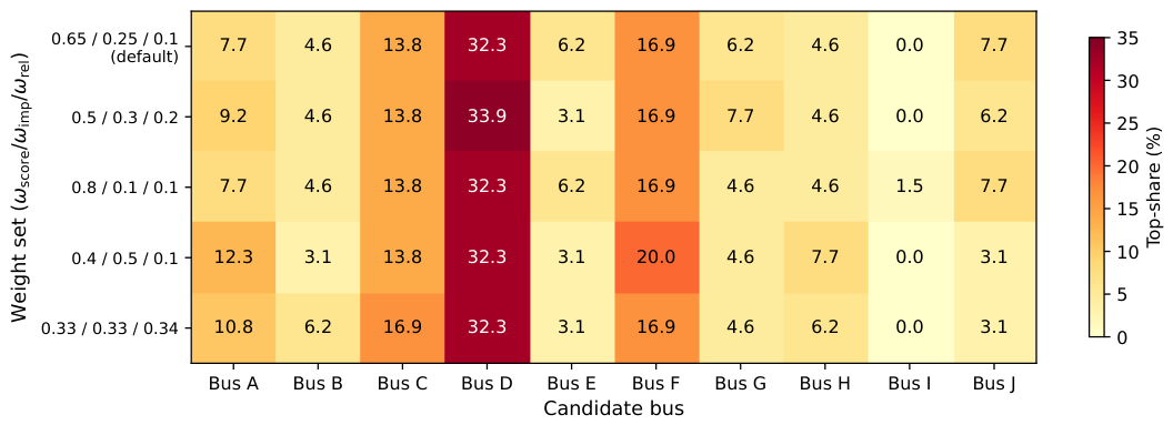
To verify that the headline ranking is not an artifact of the default weight $(0.65,0.25,0.10)$, Table 7 reports the scenario-level top-share under five representative weight configurations, recomputed off-line from the saved per-scenario rank data without re-running the power-flow engine.

Table 7. Scenario-level top-ranked share (%) under five weight configurations. Column headers A–J denote Bus A–Bus J as defined in Table 1.

Weight Set (${\mathit{\omega }}_{\mathbf{score}}/{\mathit{\omega }}_{\mathbf{imp}}/{\mathit{\omega }}_{\mathbf{rel}}$)	A	B	C	D	E	F	G	H	I	J
0.65/0.25/0.10 (default)	7.7	4.6	13.9	32.3	6.2	16.9	6.2	4.6	0.0	7.7
0.50/0.30/0.20	9.2	4.6	13.8	33.8	3.1	16.9	7.7	4.6	0.0	6.2
0.80/0.10/0.10	7.7	4.6	13.8	32.3	6.2	16.9	4.6	4.6	1.5	7.7
0.40/0.50/0.10	12.3	3.1	13.8	32.3	3.1	20.0	4.6	7.7	0.0	3.1
0.33/0.33/0.34	10.8	6.2	16.9	32.3	3.1	16.9	4.6	6.2	0.0	3.1

Figure 4 confirms that Bus D leads in every tested weighting and that the same top-3 (Bus D, Bus F, and Bus C) holds across all configurations.

Figure 4. Heatmap of scenario-level top-share (%) per candidate bus under five weight configurations of the robust score $\mathrm{RS}\left(k\right)$.

4.5. Cost-Ratio Sensitivity ($c_{\mathrm{ESS}}:c_{\mathrm{STATCOM}}$)

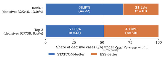
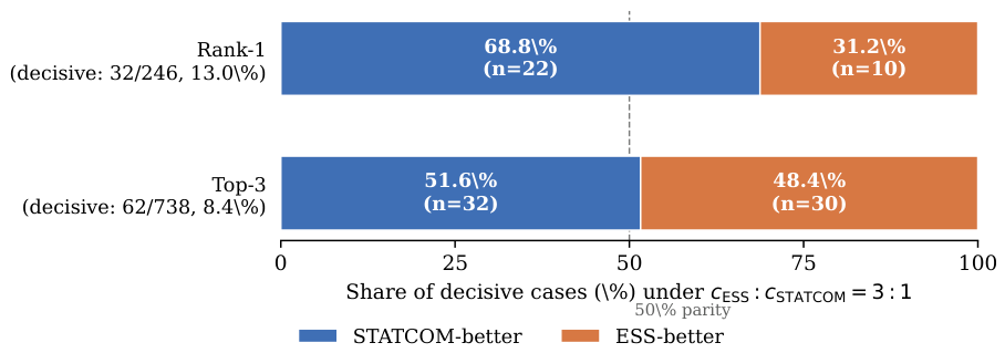
The economic comparison is evaluated under the cost-comparison proxy with an ESS-to-STATCOM unit-cost ratio of $3:1$, restricted to the decisive subset. The denominator flow is 65 scenario files into coverage accounting, 60 retain a full $(P,Q)$ sweep (the 5 excluded scenarios are lost to solver failures or active pruning), 246 valid Rank-1 rows are pooled across those 60 scenarios, and 32 are decisive after neutral ties are removed. The matching Top-3 denominator is $246\times 3=738$ rows, of which 62 are decisive. Among the decisive Rank-1 cases, STATCOM is preferred in 22 ($68.8\%$) and ESS in 10 ($31.2\%$). Among the decisive Top-3 rows, the split is nearly even (32, $51.6\%$ STATCOM-better and 30, $48.4\%$ ESS-better). Figure 5 visualizes the decisive subset. The decisive ESS-versus-STATCOM split at the $3:1$ proxy is tabulated in Appendix Table A3; because that split shifts with the assumed cost ratio only through the sizing step, a systematic sweep over other ratios is left to future work.

Figure 5. Breakdown of decisive Rank-1 ($n=32$) and Top-3 ($n=62$) economic-comparison outcomes under $c_{\mathrm{ESS}}:c_{\mathrm{STATCOM}}=3:1$.

4.6. Coverage and the Identification of Structurally Unsolvable Contingencies

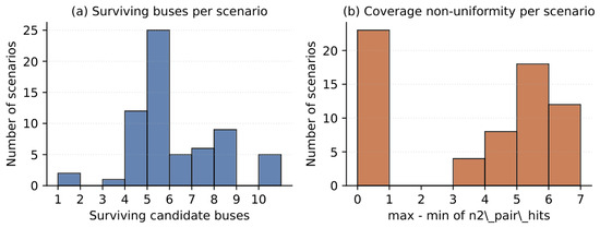
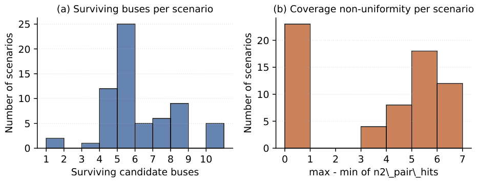
The weight and cost-ratio analyses above assume comparable per-candidate footing, so the cases in which a candidate bus drops out of the surviving rank table deserve explicit interpretation. Of the 65 scenario files analyzed, 60 (the set used by the single-pair baseline in Section 4.7) retain a complete per-candidate $(P,Q)$ sweep but contain fewer than the full 10 candidate buses in the surviving rank table because of solver non-convergence, timeouts, or active screening pruning. The remaining 5 are dropped (denominator flow given in Section 4.5). Within the 60 retained scenarios, 42 exhibit a non-uniform n2_pair_hits distribution, with the 2033 peak files most affected (per-bus range 1–7 in five of seven files). These coverage diagnostics are tabulated in Appendix Table A5.

These drop-outs are not an algorithmic artifact to be discounted. They are themselves a result. When a candidate fails to yield a feasible post-contingency operating point for a given N-2 pair—even under the near-unlimited single-bus injection permitted by the extreme search bounds of Section 3.5—the appropriate reading is that the pair is structurally unsolvable by single-node compensation, not that the candidate is poorly evaluated. Restricting the scenario-level comparison to the candidates that remain feasible across a pair set is therefore a deliberate and methodologically appropriate screening step. It ranks the realizable alternatives against one another, while the eliminated cases separately flag the contingencies for which no single-node corrective alternative exists. The two outputs answer different planning questions—where to site support, and which contingencies require structural reinforcement instead—and must not be conflated. Excluding these unmitigable contingencies from the scenario-level ranking prevents the distortion of corrective-support performance metrics, ensuring that candidates are judged only on problems that single-node compensation can actually solve.

Figure 6 presents the joint distribution of surviving candidates and n2_pair_hits spread. Because the surviving pool is non-uniform, the scenario-level top-share figures in Table 5 should be read jointly with this coverage information, and a candidate that remains feasible on only one or two N-2 pairs should not be placed on the same footing as one that remains feasible on all pairs. A natural extension is to re-execute the non-converged cases with an extended solver budget so that the surviving pool becomes uniform and the structurally unsolvable pairs can be isolated with certainty. Per-scenario coverage flags are released in the Supplementary File v7_supp_coverage.csv.

Figure 6. Coverage diagnostics. (a) Distribution of the number of surviving candidate buses per scenario. (b) Distribution of $\max -\min$ of n2_pair_hits within each scenario.

4.7. Comparison with a Single Severe-Pair Baseline

The coverage diagnostics above establish that the scenario-level ranking is internally robust within the surviving pool. To check that scenario averaging is operationally distinguishable from the conventional single-case approach, the proposed ranking is compared against a baseline that selects the corrective-support bus from the single worst N-2 pair per scenario. Across the 60 scenarios, the two procedures agree on the headline candidate in 50 ($83.3\%$) and disagree in 10 ($16.7\%$). Within each scenario only $73.0\%$ of N-2 pairs yield the same per-pair winner as the scenario-averaged winner on average. Disagreements concentrate in the 2033 peak/middle and 2026 peak/middle cases with the second-line modification.

4.8. Reliability and Failure Handling

The reliability observations are summarized in Table 8. Most failures originate from the computational burden of the all-scenario optimization stage and are concentrated in the 2033 peak cases. The refined re-analysis stage reconstructs recoverable cases, but the final results contain only surviving candidates. Hence, rows with fail_cases=0 and reliability 1.0 do not imply that no failures occurred in the original experiment.

Table 8. Reliability and failure-handling summary.

Item	Observation	Implication
Source	Original runs jointly evaluate all N-2 pairs and search points.	Burden increases sharply in stressed scenarios.
Peak	Failures occur mainly in 2033 peak cases.	Scenario hardness dominates, not a single modeling bug.
Retry	Timeouts selectively retried, and unstable pairs excluded from aggregation.	Final results reflect refined survivors rather than raw failures.
Coverage	In 2033 peak files, n2_pair_hits ranges from 1 to 7 across surviving candidates.	Coverage differences remain part of the reliability outcome.

Table 8 indicates that reliability and coverage are empirical outcomes of the repeated AC power-flow evaluation and must be interpreted alongside average performance. Candidate quality should not be judged on average performance alone.

5. Discussion

This section interprets the ranking results along three lines. Section 5.1 explains why the pair-level winner and the scenario-level robust winner identify different buses, drawing on the inland backbone topology and the HVDC state. Section 5.2 reads the residual-difficulty layer as a corridor-level vulnerability signal that points to where additional grid reinforcement is required. Section 5.3 revisits the ESS-versus-STATCOM verdict under the three-to-one cost proxy and discusses sensitivity to the assumed ratio.

5.1. Divergence Between Pair-Level and Scenario-Level Rankings

Pair-level performance and scenario-level robustness identify different buses, and the divergence is structural. Bus C excels at pair-level rankings because it influences many redistribution paths, but its diffuse connectivity does not concentrate benefit on any particular dominant stress corridor. Buses on the structural bottleneck (the inland backbone from 2026 onward, occupied by Bus D and Bus F) provide more consistent per-scenario benefit. The HVDC operating state is the most influential switching factor, changing the scenario-level winner in 10 of 16 matched on/off pairs. This also explains the ESS–STATCOM split. Pair-level dominance of an active-power-sensitive hub suggests ESS drives per-pair benefit, while the scenario-level emergence of Bus F alongside Bus D indicates STATCOM becomes relatively more important once voltage stress is evaluated across diverse scenarios. Conventional single-case studies therefore systematically favor hubs and underweight structural-bottleneck buses, the candidates that matter most under long-term horizons.

5.2. Corridor-Level Vulnerability and Planning Implications

The vulnerable-pair results provide a complementary planning signal. Bus A–Bus F and Bus I–Bus J represent different threat profiles—the former is the most frequently worst pair, the latter the most persistently difficult—so corridor-level vulnerability assessment requires both a worst-case representative pair and a persistence-based difficulty measure. A corridor that remains high-difficulty even after optimal corrective support signals that no single-point injection can compensate for the structural deficit, suggesting more fundamental reinforcement (new line, series compensation, or topology change) [7,30]. This two-layer interpretation—scenario-robust corrective siting plus corridor-level vulnerability for reinforcement—is aligned with two-stage frameworks that separate operational dispatch from structural reinforcement decisions [31], and with scenario-based cost-allocation frameworks for renewables-driven transmission expansion [4].

5.3. ESS vs. STATCOM Selection Under the $3:1$ Cost Proxy

The cost-ratio result of Section 4.5 merits separate consideration. Neutral comparisons constitute a no-decision outcome of the proxy rather than a physical equivalence claim. Within the decisive subset ($n=32$ Rank-1; $n=62$ Top-3), STATCOM dominates at Rank-1 ($68.8\%$) while the Top-3 split is nearly even. The pair-level intuition that ESS is the leading corrective resource does not consistently translate into an economic preference under a cost burden, and the recommendation is sensitive to the assumed ratio. The present paper therefore reports both the neutral count and the decisive split so that downstream studies can re-evaluate under their own cost assumptions. The ranked buses are pre-screening candidates for subsequent dynamic security assessment—transient, voltage, and frequency stability, which a static power flow cannot certify—rather than final deployment sites, so the ranking narrows the decision to a short list that is then carried into the more expensive time-domain studies. The measured computational cost and a projection to a larger system are reported in Supplementary Table S6, and the same pipeline applied unchanged to an independent IEEE 118-bus system (Supplementary Table S7) reproduces the two-layer structure of a robust siting winner plus a residual-difficulty layer. As future work, we will re-run the per-bus sizing under a range of ESS-to-STATCOM cost ratios—for example $2:1$, $4:1$, and $5:1$—to test how sensitive the STATCOM-leaning verdict is to the assumed ratio.

6. Conclusions

We propose an optimal and robust siting and ranking framework for ESS and STATCOM under 765 kV double-circuit N-2 contingencies. The framework constructs valid N-2 pairs, screens candidate buses at the 765 kV level under a fixed reference capacity, sizes ESS and STATCOM support through independent active- and reactive-power capacity sweeps, and re-ranks candidates with the integrated robust score $\mathrm{RS}\left(k\right)$ under a fixed economic-weight ratio (ESS : STATCOM $=3:1$). The framework finds optimal and robust solutions by repeating static post-contingency AC power-flow evaluations over a multi-year scenario set (2023/2026/2033) covering multiple load levels, planning conditions, and HVDC states. The pair-level best-performing bus does not coincide with the scenario-level robust winner. For example, Bus C dominates at the pair-level (48.6%), whereas Bus D (32.3%) and Bus F (16.9%) lead at the scenario-level. This divergence is structural, since Bus D and Bus F sit on the inland backbone that becomes the dominant stress path once HVDC is in service. HVDC on/off changes the scenario-level winner in 10 of 16 matched pairs. Furthermore, the residual-difficulty layer identifies Bus A–Bus F as the representative worst pair and Bus I–Bus J as the most persistent high-difficulty pair.

Three robustness diagnostics support the top three option. The Five-weight sensitivity in Table 7 keeps Bus D first in every tested configuration, including a score-dominant weight $(0.80/0.10/0.10)$ and equal weighting of equal-thirds $(0.33/0.33/0.34)$. The bootstrap 95% CI in Table 5 separate the top-3 of the scenario-level from the lower group. Under the $c_{\mathrm{ESS}}:c_{\mathrm{STATCOM}}=3:1$ proxy, 32 of 246 Rank-1 comparisons are economically decisive as STATCOM $68.8\%$ and ESS $31.2\%$, with the 62 decisive Top-3 rows split nearly evenly as $51.6\%$ and $48.4\%$. A coverage diagnostic, whose 60 of 65 scenarios end with fewer than 10 survived candidates, is reported alongside the rankings, and candidate drop-outs are explicitly excluded from the robust candidate ranking. Contingencies that do not reach a feasible post-contingency state even at the extreme 4000 MW/Mvar injection limit are identified as structurally unsolvable by single-node compensation. This indicates that they require fundamental grid reinforcement rather than operational corrective support. The four directions extend naturally. First, our framework embeds the screening and ranking layer into a multi-resource investment-optimization model that jointly sizes ESS, STATCOM, and demand-side response resources, under an explicit cost objective. Therefore, it turns the present comparison between ESS and STATCOM into a portfolio decision that minimizes costs [32]. Second, the framework also provides candidate-bus ranking, per-resource sensitivity, and a set of structurally unsolvable contingencies, so it constitutes the optimization model, the demand-side resource, and the associated economic analysis. Third, it adds dynamic indicators, which are transient stability, short-circuit ratio, and frequency nadir, to replace the set of deterministic scenarios with a probabilistic distribution to allow chance-constrained or robust extensions of $\mathrm{RS}\left(k\right)$. Fourth, it uses the vulnerable-pair signal as a seed set for line-addition, series-compensation, or topology-change studies in the 765   kV backbone.

References

- Kim, S.; Kim, H.; Lee, H.; Lee, J.; Lee, B.; Jang, G.; Lan, X.; Kim, T.; Jeon, D.; Kim, Y.; et al. Expanding power systems in the Republic of Korea: Feasibility studies and future challenges. IEEE Power Energy Mag. 2019, 17, 61–72. [Google Scholar] [CrossRef] [Scilit]
- Papic, M.; Bell, K.; Chen, Y.; Dobson, I.; Fonte, L.; Haq, E.; Hines, P.; Kirschen, D.; Luo, X.; Miller, S.S.; et al. Survey of tools for risk assessment of cascading outages. In Proceedings of the 2011 IEEE Power and Energy Society General Meeting, Detroit, MI, USA, 24–28 July 2011; pp. 1–9. [Google Scholar] [CrossRef] [Scilit]
- Morales, J.M.; Conejo, A.J.; Madsen, H.; Pinson, P.; Zugno, M. Integrating Renewables in Electricity Markets: Operational Problems; Springer: New York, NY, USA, 2014. [Google Scholar] [CrossRef] [Scilit]
- Go, Y.; Choi, W.; Kim, M.; Chung, J.-H.; Kim, H.; Lee, D. Fair transmission expansion cost allocation for renewable energy resource interconnection based on stochastic cooperative game theory. Mathematics 2025, 13, 3898. [Google Scholar] [CrossRef] [Scilit]
- Korea Electric Power Corporation. Transmission and Distribution Business: Transmission and Substation Facility Overview. 2024. Available online: https://home.kepco.co.kr/ (accessed on 31 March 2026).
- Jeong, I.; Oh, S.; Song, J.; Ku, H.; Bae, M.; Kwak, E.-S.; Min, J.-H.; Shin, J. A study on analysis of margin of transient stability and calculation of power generation constraints according to renewable energy sources in the East Coast. Trans. Korean Inst. Electr. Eng. 2022, 71, 1564–1570. [Google Scholar] [CrossRef] [Scilit]
- Conejo, A.J.; Baringo, L.; Kazempour, S.J.; Siddiqui, A.S. Investment in Electricity Generation and Transmission: Decision Making Under Uncertainty; Springer: Cham, Switzerland, 2016. [Google Scholar] [CrossRef] [Scilit]
- Abdi, H. A survey of combined heat and power-based unit commitment problem: Optimization algorithms, case studies, challenges, and future directions. Mathematics 2023, 11, 4170. [Google Scholar] [CrossRef] [Scilit]
- Davis, C.M.; Overbye, T.J. Multiple element contingency screening. IEEE Trans. Power Syst. 2011, 26, 1294–1301. [Google Scholar] [CrossRef] [Scilit]
- Kaplunovich, P.; Turitsyn, K. Fast and reliable screening of N-2 contingencies. IEEE Trans. Power Syst. 2016, 31, 4243–4252. [Google Scholar] [CrossRef] [Scilit]
- Aguado, J.A.; de la Torre, S.; Triviño, A. Battery energy storage systems in transmission network expansion planning. Electr. Power Syst. Res. 2017, 145, 63–72. [Google Scholar] [CrossRef] [Scilit]
- Lindner, M.; Peper, J.; Offermann, N.; Biele, C.; Teodosic, M.; Pohl, O.; Menne, J.; Häger, U. Operation strategies of battery energy storage systems for preventive and curative congestion management in transmission grids. IET Gener. Transm. Distrib. 2023, 17, 589–603. [Google Scholar] [CrossRef] [Scilit]
- Khani, H.; Dadash Zadeh, M.R.; Hajimiragha, A.H. Transmission congestion relief using privately owned large-scale energy storage systems in a competitive electricity market. IEEE Trans. Power Syst. 2016, 31, 1449–1458. [Google Scholar] [CrossRef] [Scilit]
- Jung, S.-W.; An, Y.-Y.; Suh, B.; Park, Y.; Kim, J.; Kim, K.-I. Multi-agent deep reinforcement learning for scheduling of energy storage system in microgrids. Mathematics 2025, 13, 1999. [Google Scholar] [CrossRef] [Scilit]
- Xu, Y.; Dong, Z.Y.; Xiao, C.; Zhang, R.; Wong, K.P. Optimal placement of static compensators for multi-objective voltage stability enhancement of power systems. IET Gener. Transm. Distrib. 2015, 9, 2144–2151. [Google Scholar] [CrossRef] [Scilit]
- Kundur, P.; Paserba, J.; Ajjarapu, V.; Andersson, G.; Bose, A.; Canizares, C.; Hatziargyriou, N.; Hill, D.; Stankovic, A.; Taylor, C.; et al. Definition and classification of power system stability IEEE/CIGRE Joint Task Force on Stability Terms and Definitions. IEEE Trans. Power Syst. 2004, 19, 1387–1401. [Google Scholar] [CrossRef] [Scilit]
- Bai, W.; Lee, D.; Lee, K.Y. Stochastic dynamic AC optimal power flow based on a multivariate short-term wind power scenario forecasting model. Energies 2017, 10, 2138. [Google Scholar] [CrossRef] [Scilit]
- Bhattacharya, A.; Chakraborty, A.K.; Bhattacharjee, A. Dynamic security assessment of power systems: A comprehensive review of computational intelligence techniques. Int. J. Electr. Power Energy Syst. 2020, 121, 106126. [Google Scholar] [CrossRef] [Scilit]
- Chakraborty, A.; Musunuri, S.K.; Srivastava, A.K.; Kondabathini, A.K. Integrating STATCOM and battery energy storage system for power system transient stability. Adv. Power Electron. 2012, 2012, 676010. [Google Scholar] [CrossRef] [Scilit]
- Ejebe, G.C.; Wollenberg, B.F. Automatic contingency selection. IEEE Trans. Power Appar. Syst. 1979, PAS-98, 97–109. [Google Scholar] [CrossRef] [Scilit]
- Ministry of Trade, Industry and Energy. Standard for Reliability and Quality of Electricity in Power Systems; MOTIE Notification No. 2023-65. Ministry of Trade, Industry and Energy: Sejong, Republic of Korea, 2023. Available online: https://www.law.go.kr/admRulLsInfoP.do?admRulSeq=69497 (accessed on 15 May 2026).
- Cole, W.; Ramasamy, V.; Turan, M. Cost Projections for Utility-Scale Battery Storage: 2025 Update; NREL/TP-6A40-93281. National Renewable Energy Laboratory: Golden, CO, USA, 2025.
- Carbonara, A.; Dambone Sessa, S.; L’Abbate, A.; Sanniti, F.; Chiumeo, R. Comparison of advanced flexible alternating current transmission system (FACTS) devices with conventional technologies for power system stability enhancement: An updated review. Electronics 2024, 13, 4262. [Google Scholar] [CrossRef] [Scilit]
- Hooke, R.; Jeeves, T.A. Direct search solution of numerical and statistical problems. J. ACM 1961, 8, 212–229. [Google Scholar] [CrossRef] [Scilit]
- Kollenda, K.; Schrief, A.; Biele, C.; Lindner, M.; Sundorf, N.; Hoffrichter, A.; Roehder, A.; Moser, A.; Rehtanz, C. Curative measures identification in congestion management exploiting temporary admissible thermal loading of overhead lines. IET Gener. Transm. Distrib. 2022, 16, 3171–3183. [Google Scholar] [CrossRef] [Scilit]
- Yager, R.R. On ordered weighted averaging aggregation operators in multicriteria decisionmaking. IEEE Trans. Syst. Man Cybern. 1988, 18, 183–190. [Google Scholar] [CrossRef] [Scilit]
- Ben-Tal, A.; El Ghaoui, L.; Nemirovski, A. Robust Optimization; Princeton Series in Applied Mathematics; Princeton University Press: Princeton, NJ, USA, 2009. [Google Scholar] [CrossRef] [Scilit]
- Wang, Z.; Cao, R.; Tang, D.; Wang, C.; Liu, X.; Hu, W. Distributionally robust energy optimization with renewable resource uncertainty. Mathematics 2025, 13, 992. [Google Scholar] [CrossRef] [Scilit]
- Efron, B.; Tibshirani, R. Bootstrap methods for standard errors, confidence intervals, and other measures of statistical accuracy. Stat. Sci. 1986, 1, 54–75. [Google Scholar] [CrossRef] [Scilit]
- Fisher, E.B.; O’Neill, R.P.; Ferris, M.C. Optimal transmission switching. IEEE Trans. Power Syst. 2008, 23, 1346–1355. [Google Scholar] [CrossRef] [Scilit]
- Zhou, B.; Xu, D.; Chan, K.W.; Li, C.; Cao, Y.; Bu, S. A two-stage framework for multiobjective energy management in distribution networks with a high penetration of wind energy. Energy 2017, 135, 754–766. [Google Scholar] [CrossRef] [Scilit]
- Aghaei, J.; Amjady, N.; Shayanfar, H.A. Multi-objective electricity market clearing considering dynamic security by lexicographic optimization and augmented epsilon constraint method. Appl. Soft Comput. 2011, 11, 3846–3858. [Google Scholar] [CrossRef] [Scilit]
Disclaimer/Publisher’s Note: The statements, opinions and data contained in all publications are solely those of the individual author(s) and contributor(s) and not of MDPI and/or the editor(s). MDPI and/or the editor(s) disclaim responsibility for any injury to people or property resulting from any ideas, methods, instructions or products referred to in the content. |
© 2026 by the authors. Licensee MDPI, Basel, Switzerland. This article is an open access article distributed under the terms and conditions of the Creative Commons Attribution (CC BY) license.