Global Dynamics of Population–Toxin Systems with Nonlocal Usage of Memory Under Periodic Boundary Conditions

Abstract

We study a reaction–diffusion model for population–toxin interactions on a two-dimensional torus, where avoidance is driven by a nonlocal average of toxin-related memory. The variables represent population density, toxin concentration, and a phenomenological information field generated by population–toxin encounters. This information diffuses, decays, and enters the taxis term through convolution with a perceptual kernel. We prove local well-posedness, global existence and uniform boundedness, and give sufficient conditions for exponential convergence to either the positive equilibrium or the toxin-only equilibrium. Numerical simulations with two perceptual radii yield stripe and spot patterns, illustrating that the sensing scale can alter spatial organization. These simulations do not establish an effect on population persistence and should be viewed as hypotheses for empirical study.

1. Introduction

1.1. The Model

Toxicants can alter reproduction, mortality, and movement, thereby changing the abundance and spatial distribution of exposed populations [1,2,3,4,5]. Their effects may propagate through interacting populations and, under sustained exposure, contribute to local population loss. Reaction–diffusion models provide a natural setting in which demographic processes, dispersal, and environmental stress can be studied together [6,7,8,9].

Movement need not depend only on conditions at an individual’s current location. Chemical, visual, and social cues can convey information acquired at other locations or earlier times, allowing animals to avoid contaminated regions or locate resources [10,11,12,13,14,15]. Such spatially distributed information motivates models in which movement responds to a nonlocal signal rather than solely to the contemporaneous local toxin concentration [16].

Reaction–diffusion and taxis models have been used to describe contaminated environments. Huang et al. [2] and Shan and Huang [17] analyzed toxin-dependent population interactions, with emphasis on the direct demographic effects of toxicants. Deng et al. [18] and Xing et al. [19] incorporated avoidance of toxicants and studied global dynamics, bistability, and pattern formation. In those systems, movement is driven by the current local toxicant field; there is no separate information state used over a spatial neighborhood.

Keller–Segel-type systems supply much of the analytical background for taxis-driven aggregation and pattern formation [7,20]. Bellomo et al. [20] reviewed mechanisms that prevent blow-up, whereas Xu et al. [21] studied finite-speed propagation under degenerate diffusion. These studies identify difficulties caused by taxis, but they do not include toxin-related memory.

Nonlocal perception and spatial memory appear in several ecological movement models. Potts and Lewis [22], Wang and Salmaniw [16], and Painter et al. [23] considered movement based on spatially averaged information and its role in aggregation or pattern formation. Song et al. [24] and Xue et al. [25] examined detection scales, stability, and bifurcation in cognitive or memory-based systems, while Bo et al. [26] studied bifurcation in a cognitive population model for a toxic environment. The closest analytical precedent is the cognitive consumer–resource model of Zhang et al. [15], for which global solvability and stability were established. Here the resource equation is replaced by an externally supplied toxin that is depleted by the population, and the analysis covers both coexistence and toxin-only equilibria under periodic boundary conditions.

The contribution is therefore specific to the population–toxin feedback considered here: exposure generates an information field, and a nonlocal average of this field drives avoidance. We establish well-posedness and uniform boundedness, derive sufficient conditions and convergence rates for two equilibria, and examine the effect of perceptual radius on the simulated spatial distribution. Periodic boundary conditions remove boundary fluxes from this analysis.

We consider the following reaction–diffusion system on a two-dimensional torus:

$$\begin{array}{c}\hfill \left\{\begin{array}{cc}{u}_t=d_1\Delta u+\chi \nabla ·\left(u\nabla \widehat{z}\right)+ru\left(1-{\displaystyle \frac{u}{K}}\right)-auv,\hfill & x\in U,t>0,\\ v_t=d_2\Delta v+h-\beta v-\eta uv,\hfill & x\in U,t>0,\\ z_t=d_3\Delta z+buv-\gamma z,\hfill & x\in U,t>0,\\ u(x,0)=u_0(x),v(x,0)=v_0(x),z(x,0)=z_0(x),\hfill & x\in U,t=0,\end{array}\right.\end{array}$$

(1)

where $U={\mathbb{R}}^2/L{\mathbb{Z}}^2\cong {\left(-{\displaystyle \frac{L}{2}},{\displaystyle \frac{L}{2}}\right)}^2$ is a torus of side length $L>0$, with periodic boundary conditions. The variables u, v, and z denote population density, toxin concentration, and toxin-related information, respectively. The convolution $\widehat{z}=G\ast z$ is the spatially averaged information used in the taxis term. The parameters r and K are the intrinsic growth rate and carrying capacity; a is the toxin-induced mortality rate; h, $\beta$, and $\eta$ are the toxin input, decay, and population uptake rates; and b and $\gamma$ are the production and decay rates of toxin-related information. The diffusion coefficients of u, v, and z are $d_1$, $d_2$, and $d_3$.

The equation for z is phenomenological. Its source $buv$ assumes that information is generated when the population and toxin co-occur, with b converting exposure into shared information. The terms $d_3\Delta z$ and $-\gamma z$ describe spatial transmission and loss of information. This production–transmission–decay structure is consistent with models of memory-dependent movement and collective sensing [16,27,28,29]. Accordingly, z is an aggregate information state, not a directly measured physiological concentration.

The field $\widehat{z}=G\ast z$ averages information over a perceptual neighborhood. The term $\chi \nabla ·(u\nabla \widehat{z})$ represents movement away from locations with larger perceived toxin information, following the use of nonlocal signals in collective-movement and spatial-memory models [22,30].

More precisely, $\widehat{z}(x,t)={\int }_{U}z(y,t)G(x-y)dy$, where $G(x-y)$ weights information at displacement $x-y$. We impose the following assumptions on the kernel:

(H1)

$G\in L^1(U)\cap L^{\infty }(U)$, with a constant $G_0>0$ such that ${max\{\parallel G\parallel }_{L^1}{,\parallel G\parallel }_{L^{\infty }}\}\le G_0$.

(H2)

There exists $C_G>0$ such that for all smooth $\varphi$, ${\parallel \nabla G\ast \varphi \parallel }_{L^1(U)}\le C_G{\parallel \varphi \parallel }_{L^1(U)}$, or equivalently, $G\in \mathrm{BV}(U)$ with total variation ${\parallel \nabla G\parallel }_{\mathrm{TV}}<C_{TV}<\infty$, where $\mathrm{BV}(U)$ is the space of functions of bounded variation.

(H3)

$G(x-y)>0$, $G(x-y)=G(y-x)$, and ${\int }_{U}G(x-y)dy=1$ for $x,y\in U$.

(H4)

G is compactly supported.

We specifically consider the perceptual kernel

$$\begin{array}{c}\hfill G(x-y):=\left\{\begin{array}{cc}{\displaystyle \frac{1}{\pi R^2}},\hfill & \parallel x-y\parallel \le R,\hfill \\ 0,\hfill & \mathrm{otherwise},\hfill \end{array}\right.\end{array}$$

(2)

where $\parallel x-y\parallel$ is the Euclidean distance and $R\ge 0$ is the perceptual range. For some $\alpha \in (0,1)$, the initial data satisfy

$$\left\{\begin{array}{c}{u}_0(x)\in C^{2+\alpha }(U),u_0(x)>0\mathrm{in}U,\hfill \\ v_0(x)\in C^{2+\alpha }(U),v_0(x)>0\mathrm{in}U,\hfill \\ z_0(x)\in C^{2+\alpha }(U),z_0(x)>0\mathrm{in}U.\hfill \end{array}\right.$$

(3)

1.2. Objectives and Challenges

We establish local well-posedness and global boundedness, and then derive sufficient conditions for the global asymptotic stability of the positive and toxin-only equilibria. Numerical simulations are used to examine how the perceptual range changes spatial organization. The analytical results concern the proposed model; claims about persistence or management would require empirical validation.

The principal estimate couples u and z. The population equation contains $\chi \nabla ·(u\nabla \widehat{z})$, while the information equation contains the source $buv$. A bound for u therefore requires control of derivatives of $\widehat{z}=G\ast z$, which in turn depends on the regularity available for z. The taxis term also prevents a direct application of the scalar maximum principle to the u-equation. These features require joint energy and semigroup estimates rather than separate estimates for the three components [31].

Two points require particular care:

(i)

The taxis term contains $\nabla \widehat{z}$, the gradient of a convolution. Higher-order estimates must accommodate the limited regularity $G\in BV(U)$, rather than assuming a smooth kernel such as $G\in C^2(U)$ [32].

(ii)

Global continuation requires uniform control of the norms in the extensibility criterion. Taxis may concentrate the population even when movement is directed away from toxin, so the proof must combine diffusion, logistic damping, and decay to rule out loss of regularity [24].

The resulting argument combines energy inequalities, heat-semigroup estimates, interpolation, and parabolic regularity.

1.3. Main Results

The first theorem gives global existence and boundedness for (1).

Theorem 1.

Let $U={\mathbb{R}}^2/L{\mathbb{Z}}^2\cong {\left(-{\displaystyle \frac{L}{2}},{\displaystyle \frac{L}{2}}\right)}^2\subset {\mathbb{R}}^2$ be a torus of size $L>0$. For any initial data $(u_0,v_0,z_0)$ satisfying (3) and any $T>0$, system (1) has a unique solution

$$(u,v,z)\in {[C^{2+\alpha ,1+{\displaystyle \frac{\alpha }{2}}}(U\times [0,T])]}^3,$$

with

$$u>0,z>0,\mathit{and}0<v\le max\{\parallel v_0{\parallel }_{L^{\infty }(U)},{\displaystyle \frac{h}{\beta }}\}\mathrm{in}U\times (0,T).$$

The asymptotic analysis concerns the homogeneous equilibria $E_0=(0,h/\beta ,0)$ and $E^{\ast }=(u^{\ast },v^{\ast },z^{\ast })$. Their components satisfy

$$\left\{\begin{array}{c}ru\left(1-{\displaystyle \frac{u}{K}}\right)-auv=0,\hfill \\ h-\beta v-\eta uv=0,\hfill \\ buv-\gamma z=0.\hfill \end{array}\right.$$

(4)

Eliminating v from the first two equations gives

$$f(u):=r\eta u^2-(r\eta K-r\beta )u-K(r\beta -ah)=0.$$

If $r\beta >ah$, then $f(0)=-K(r\beta -ah)<0$ and $f(K)=Kah>0$. Hence, f has a unique root $u^{\ast }\in (0,K)$, namely

$$u^{\ast }={\displaystyle \frac{r(\eta K-\beta )+\sqrt{r^2{(\beta -\eta K)}^2+4r\eta K(r\beta -ah)}}{2r\eta }}.$$

The remaining components are

$$v^{\ast }={\displaystyle \frac{h}{\beta +\eta u^{\ast }}}>0,z^{\ast }={\displaystyle \frac{b{u}^{\ast }{v}^{\ast }}{\gamma }}>0.$$

The stability result is stated next.

Theorem 2.

Under the assumptions of Theorem 1, the solution $(u,v,z)$ of system (1) exhibits the following convergence:

(1) 

If condition (56) holds, then

$$(u,v,z)\to (u^{\ast },v^{\ast },z^{\ast })\mathit{exponentially}\mathit{as}t\to \infty .$$

(2) 

If condition (65) holds, then

$$(u,v,z)\to (0,{\displaystyle \frac{h}{\beta }},0)\mathit{exponentially}\mathit{as}t\to \infty .$$

Section 2 proves local existence and uniqueness. The a priori estimates in Section 3 yield global boundedness and Theorem 1. Lyapunov arguments in Section 4 establish Theorem 2, after which Section 5 examines the effect of perceptual range in numerical simulations. The final section summarizes the results and their limitations.

2. Local Existence and Uniqueness of Solutions

We first obtain a local classical solution of (1) by a fixed-point argument and record the corresponding continuation criterion.

Lemma 1.

Assume that the initial data satisfy (3) and that the perceptual kernel G satisfies (H1)–(H4). Then there is a maximal time $T_{\max }\in (0,\infty ]$ and a unique classical solution $(u,v,z)$ of (1) such that

$$(u,v,z)\in {\left[C^{2+\alpha ,1+\alpha /2}(U\times [0,T_{\max }))\right]}^3,$$

(5)

for some $\alpha \in (0,1)$, with $u,v,z>0$ in $U\times [0,T_{\max })$. If $T_{\max }<\infty$, then

$$\underset{t\to T_{\max }^{-}}{lim\; sup}\left({\parallel u(·,t)\parallel }_{C^{2+\alpha }}+{\parallel v(·,t)\parallel }_{C^{2+\alpha }}+{\parallel z(·,t)\parallel }_{C^{2+\alpha }}\right)=\infty .$$

(6)

Proof. 

We construct a fixed point, verify that the defining map is contractive for small time, and then give an energy proof of uniqueness.

(i) Existence. Write the nonlinear terms in (1) as

$$\left\{\begin{array}{c}{f}_u(u,v,\widehat{z})=\chi \nabla ·(u\nabla \widehat{z})+ru\left(1-{\displaystyle \frac{u}{K}}\right)-auv,\hfill \\ f_v(u,v)=h-\beta v-\eta uv,\hfill \\ f_z(u,v,z)=buv-\gamma z,\hfill \end{array}\right.$$

where $\widehat{z}(x,t)={\int }_{U}z(y,t)G(x-y)dy$.

We define the solution space for a time interval $[0,T]$ as

$$X_T={\left[C^{2+\alpha ,1+\alpha /2}(U\times [0,T])\right]}^3,$$

equipped with the norm

$$\begin{array}{cc}\hfill {\parallel (u,v,z)\parallel }_{X_T}=& {\parallel u\parallel }_{C^{2+\alpha ,1+\alpha /2}}+{\parallel v\parallel }_{C^{2+\alpha ,1+\alpha /2}}\hfill \\ \hfill & +{\parallel z\parallel }_{C^{2+\alpha ,1+\alpha /2}}.\hfill \end{array}$$

where $\alpha \in (0,1)$ is determined by the regularity of the initial data $u_0,v_0,z_0\in C^{2+\alpha }(U)$. Define the closed subset

$$\begin{array}{cc}\hfill S_T=\{(u,v,z)\in X_T:& {\parallel u\parallel }_{C^{2+\alpha ,1+\alpha /2}}\le M,{\parallel v\parallel }_{C^{2+\alpha ,1+\alpha /2}}\le M,\hfill \\ \hfill & {\parallel z\parallel }_{C^{2+\alpha ,1+\alpha /2}}\le M,u,v,z\ge {\delta }_0\}.\hfill \end{array}$$

Here $M>max\{\parallel u_0{\parallel }_{C^{2+\alpha }},\parallel v_0{\parallel }_{C^{2+\alpha }},\parallel z_0{\parallel }_{C^{2+\alpha }}\}$, and ${\delta }_0>0$ is chosen below the initial infima so that positivity is retained for short time.

We construct the mapping $\Phi :S_T\to X_T$, defined by $\Phi (\tilde{u},\tilde{v},\tilde{z})=(u,v,z)$, where $(u,v,z)$ solves

$$\left\{\begin{array}{cc}{\partial }_{t}u-d_1\Delta u=f_u(\tilde{u},\tilde{v},\tilde{\widehat{z}}),\hfill & u(x,0)=u_0(x),\hfill \\ {\partial }_{t}v-d_2\Delta v=f_v(\tilde{u},\tilde{v}),\hfill & v(x,0)=v_0(x),\hfill \\ {\partial }_{t}z-d_3\Delta z=b\tilde{u}\tilde{v}-\gamma \tilde{z},\hfill & z(x,0)=z_0(x),\hfill \end{array}\right.$$

with $\tilde{\widehat{z}}=G\ast \tilde{z}$. We show that $\Phi (S_T)\subset S_T$ when $T>0$ is sufficiently small.

We begin with the u-equation. Since $\tilde{u},\tilde{z}\in C^{2+\alpha ,1+\alpha /2}$ have norms bounded by M, the convolution $\tilde{\widehat{z}}=G\ast \tilde{z}$ satisfies

$$\parallel \tilde{\widehat{z}}{\parallel }_{C^{k+\alpha }}\le {\parallel G\parallel }_{L^1}{\parallel \tilde{z}\parallel }_{C^{k+\alpha }}\le G_{0}M,k=0,1,2,$$

where $G_0={\parallel G\parallel }_{L^1}$. In particular, $\parallel \tilde{\widehat{z}}{\parallel }_{C^{2+\alpha }}\le G_{0}M$. For the taxis term,

$$\chi \nabla ·(\tilde{u}\nabla \tilde{\widehat{z}})=\chi (\nabla \tilde{u}·\nabla \tilde{\widehat{z}}+\tilde{u}\Delta \tilde{\widehat{z}}),$$

the Hölder product estimates give

$$\begin{array}{cc}\hfill & \parallel \nabla \tilde{u}{\parallel }_{C^{\alpha }}\le {\parallel \tilde{u}\parallel }_{C^{1+\alpha }}\le M,\hfill \\ \hfill & \parallel \nabla \tilde{\widehat{z}}{\parallel }_{C^{\alpha }}\le G_0{\parallel \nabla \tilde{z}\parallel }_{C^{\alpha }}\le G_{0}M,\hfill \\ \hfill & \parallel \nabla \tilde{u}·\nabla \tilde{\widehat{z}}{\parallel }_{C^{\alpha }}\le C\parallel \nabla \tilde{u}{\parallel }_{C^{\alpha }}{\parallel \nabla \tilde{\widehat{z}}\parallel }_{C^{\alpha }}\le C{M}^2,\hfill \\ \hfill & \parallel \tilde{u}{\parallel }_{C^{\alpha }}\le M,\hfill \\ \hfill & \parallel \Delta \tilde{\widehat{z}}{\parallel }_{C^{\alpha }}\le G_0{\parallel \Delta \tilde{z}\parallel }_{C^{\alpha }}\le G_{0}M,\hfill \\ \hfill & \parallel \tilde{u}\Delta \tilde{\widehat{z}}{\parallel }_{C^{\alpha }}\le C\parallel \tilde{u}{\parallel }_{C^{\alpha }}{\parallel \Delta \tilde{\widehat{z}}\parallel }_{C^{\alpha }}\le C{M}^2.\hfill \end{array}$$

It follows that $\parallel \chi \nabla ·(\tilde{u}\nabla \tilde{\widehat{z}}){\parallel }_{C^{\alpha }}\le C{M}^2$. The reaction terms satisfy

$$\parallel r\tilde{u}(1-\tilde{u}/K){\parallel }_{C^{\alpha }}\le CM(1+M/K)\le C{M}^2,{\parallel a\tilde{u}\tilde{v}\parallel }_{C^{\alpha }}\le a{M}^2.$$

Hence, $\parallel f_u{\parallel }_{C^{\alpha ,\alpha /2}}\le C{M}^2$. The parabolic Schauder estimate gives

$${\parallel u\parallel }_{C^{2+\alpha ,1+\alpha /2}}\le C_S\left(\parallel u_0{\parallel }_{C^{2+\alpha }}+T^{\theta }{\parallel f_u\parallel }_{C^{\alpha ,\alpha /2}}\right)\le C_S\left(\parallel u_0{\parallel }_{C^{2+\alpha }}+T^{\theta }C{M}^2\right).$$

Choose $M>2C_S{\parallel u_0\parallel }_{C^{2+\alpha }}$ and $T>0$ such that $C_S{T}^{\theta }C{M}^2\le M/2$, ensuring ${\parallel u\parallel }_{C^{2+\alpha ,1+\alpha /2}}\le M$.

The estimates for v and z are similar. For v,

$$\parallel f_v{\parallel }_{C^{\alpha ,\alpha /2}}\le {\parallel h\parallel }_{C^{\alpha }}+\beta \parallel \tilde{v}{\parallel }_{C^{\alpha }}+\eta {\parallel \tilde{u}\tilde{v}\parallel }_{C^{\alpha }}\le C(1+M^2).$$

Thus, ${\parallel v\parallel }_{C^{2+\alpha ,1+\alpha /2}}\le C_S\left(\parallel v_0{\parallel }_{C^{2+\alpha }}+T^{\theta }C(1+M^2)\right)$. For $M>2C_S{\parallel v_0\parallel }_{C^{2+\alpha }}$ and sufficiently small T, we ensure ${\parallel v\parallel }_{C^{2+\alpha ,1+\alpha /2}}\le M$.

For z,

$$\parallel f_z{\parallel }_{C^{\alpha ,\alpha /2}}\le b\parallel \tilde{u}\tilde{v}{\parallel }_{C^{\alpha }}+\gamma {\parallel \tilde{z}\parallel }_{C^{\alpha }}\le C{M}^2.$$

The Schauder estimate for ${\partial }_{t}z-d_3\Delta z=f_z$ yields

$${\parallel z\parallel }_{C^{2+\alpha ,1+\alpha /2}}\le C_S^{\prime }\left(\parallel z_0{\parallel }_{C^{2+\alpha }}+T^{\theta }{\parallel f_z\parallel }_{C^{\alpha ,\alpha /2}}\right)\le C_S^{\prime }\left(\parallel z_0{\parallel }_{C^{2+\alpha }}+T^{\theta }C{M}^2\right).$$

Choose $M>2C_S^{\prime }{\parallel z_0\parallel }_{C^{2+\alpha }}$ and then choose T so that $C_S^{\prime }{T}^{\theta }C{M}^2\le M/2$. This gives ${\parallel z\parallel }_{C^{2+\alpha ,1+\alpha /2}}\le M$. The constant $C_S^{\prime }$ may depend on the fixed coefficient $d_3$.

For small T, continuity from the positive initial data and the strong maximum principle give $u,v,z\ge {\delta }_0$; the source $b\tilde{u}\tilde{v}$ in the z-equation is nonnegative.

Hence, $\Phi (S_T)\subset S_T$ for the choices of M and T above.

(ii) Contraction property of $\Phi$. Take two inputs $({\tilde{u}}^i,{\tilde{v}}^i,{\tilde{z}}^i)\in S_T$, $i=1,2$, with outputs $(u^i,v^i,z^i)=\Phi ({\tilde{u}}^i,{\tilde{v}}^i,{\tilde{z}}^i)$, and define

$$\begin{array}{cc}\hfill & \delta u={\tilde{u}}^1-{\tilde{u}}^2,\delta v={\tilde{v}}^1-{\tilde{v}}^2,\delta z={\tilde{z}}^1-{\tilde{z}}^2,\delta \widehat{z}=G\ast \delta z\hfill \end{array}$$

We estimate the difference of the corresponding outputs in $X_T$.

Product estimates in Hölder spaces give

$$\begin{array}{cc}\hfill \parallel f_u^1-f_u^2{\parallel }_{C^{\alpha ,\alpha /2}}\le & CM\left({\parallel \delta u\parallel }_{C^{2+\alpha }}+{\parallel \delta z\parallel }_{C^{2+\alpha }}\right)\hfill \\ \hfill & +CM\left({\parallel \delta u\parallel }_{C^{\alpha }}+{\parallel \delta v\parallel }_{C^{\alpha }}\right)\hfill \\ \hfill \le & CM\left({\parallel \delta u\parallel }_{X_T}+{\parallel \delta v\parallel }_{X_T}+{\parallel \delta z\parallel }_{X_T}\right).\hfill \end{array}$$

The Schauder estimate gives

$$\parallel u^1-u^2{\parallel }_{C^{2+\alpha ,1+\alpha /2}}\le C_S{T}^{\theta }CM{\parallel (\delta u,\delta v,\delta z)\parallel }_{X_T}.$$

For v and z, the same argument gives

$$\begin{array}{cc}\hfill \parallel f_v^1-f_v^2{\parallel }_{C^{\alpha ,\alpha /2}}& ={∥h-\beta ({\tilde{v}}^1-{\tilde{v}}^2)-\eta ({\tilde{u}}^1{\tilde{v}}^1-{\tilde{u}}^2{\tilde{v}}^2)∥}_{C^{\alpha }}\hfill \\ \hfill & \le {CM(\parallel \delta u\parallel }_{C^{2+\alpha }}+{\parallel \delta v\parallel }_{C^{2+\alpha }}{)+CM(\parallel \delta u\parallel }_{C^{\alpha }}+{\parallel \delta v\parallel }_{C^{\alpha }})\hfill \\ \hfill & \le CM(\parallel \delta u{\parallel }_{X_T}+\parallel \delta v{\parallel }_{X_T}),\hfill \end{array}$$

and the Schauder estimate gives

$$\parallel v^1-v^2{\parallel }_{C^{2+\alpha ,1+\alpha /2}}\le C_S{T}^{\theta }CM{\parallel (\delta u,\delta v,\delta z)\parallel }_{X_T}.$$

For z,

$$\begin{array}{cc}\hfill \parallel f_z^1-f_z^2{\parallel }_{C^{\alpha ,\alpha /2}}=& {∥b({\tilde{u}}^1{\tilde{v}}^1-{\tilde{u}}^2{\tilde{v}}^2)-\gamma ({\tilde{z}}^1-{\tilde{z}}^2)∥}_{C^{\alpha }}\hfill \\ \hfill \le & CM\left({\parallel \delta u\parallel }_{C^{2+\alpha }}+{\parallel \delta v\parallel }_{C^{2+\alpha }}+{\parallel \delta z\parallel }_{C^{2+\alpha }}\right)\hfill \\ \hfill & +CM\left({\parallel \delta u\parallel }_{C^{\alpha }}+{\parallel \delta v\parallel }_{C^{\alpha }}+{\parallel \delta z\parallel }_{C^{\alpha }}\right)\hfill \\ \hfill \le & CM\left({\parallel \delta u\parallel }_{X_T}+{\parallel \delta v\parallel }_{X_T}+{\parallel \delta z\parallel }_{X_T}\right),\hfill \end{array}$$

and by Schauder estimates,

$$\parallel z^1-z^2{\parallel }_{C^{2+\alpha ,1+\alpha /2}}\le C_S^{\prime }{T}^{\theta }CM{\parallel (\delta u,\delta v,\delta z)\parallel }_{X_T}.$$

Combining these estimates gives

$$\begin{array}{cc}\hfill & \parallel \Phi ({\tilde{u}}^1,{\tilde{v}}^1,{\tilde{z}}^1)-\Phi ({\tilde{u}}^2,{\tilde{v}}^2,{\tilde{z}}^2){\parallel }_{X_T}\hfill \\ \hfill & \le C_{\mathrm{total}}{T}^{\theta }M{\parallel (\delta u,\delta v,\delta z)\parallel }_{X_T}.\hfill \end{array}$$

Choose T so that $C_{\mathrm{total}}{T}^{\theta }M<1$. Then $\Phi$ is a contraction and has a unique fixed point in $S_T$. Standard continuation gives a maximal interval $[0,T_{max})$ and the blow-up criterion (6).

(iii) Uniqueness. Assume that two classical solutions $(u^1,v^1,z^1)$ and $(u^2,v^2,z^2)$ in ${[C^{2+\alpha ,1+\alpha /2}]}^3$ have the same initial data. Define

$$U=u^1-u^2,V=v^1-v^2,Z=z^1-z^2.$$

The difference equations are

$$\left\{\begin{array}{cc}\hfill {\partial }_{t}U=& d_1\Delta U+\chi \nabla ·(u^1\nabla {\widehat{z}}^1-u^2\nabla {\widehat{z}}^2)\hfill \\ \hfill & +r\left[u^1\left(1-{\displaystyle \frac{u^1}{K}}\right)-u^2\left(1-{\displaystyle \frac{u^2}{K}}\right)\right]-a(u^1{v}^1-u^2{v}^2),\hfill \\ \hfill {\partial }_{t}V=& d_2\Delta V-\beta V-\eta (u^1{v}^1-u^2{v}^2),\hfill \\ \hfill {\partial }_{t}Z=& d_3\Delta Z+b(u^1{v}^1-u^2{v}^2)-\gamma Z.\hfill \end{array}\right.$$

Multiplying the U-equation by U and integrating by parts gives

$$\begin{array}{cc}\hfill {\displaystyle \frac{1}{2}}{\displaystyle \frac{d}{dt}}{\int }_U{U}^{2}dx=& -d_1{\int }_U{|\nabla U|}^{2}dx-\chi {\int }_U\nabla U·(u^1\nabla {\widehat{z}}^1-u^2\nabla {\widehat{z}}^2)dx\hfill \\ \hfill & +{\int }_{U}U\left[r\left(u^1\left(1-{\displaystyle \frac{u^1}{K}}\right)-u^2\left(1-{\displaystyle \frac{u^2}{K}}\right)\right)-a(u^1{v}^1-u^2{v}^2)\right]dx.\hfill \end{array}$$

For the taxis term,

$$u^1\nabla {\widehat{z}}^1-u^2\nabla {\widehat{z}}^2=u^1\nabla \widehat{Z}+U\nabla {\widehat{z}}^2.$$

$$\left|{\int }_U\nabla U·(u^1\nabla \widehat{Z})dx\right|\le {\parallel \nabla U\parallel }_{L^2}\parallel u^1{\parallel }_{L^{\infty }}\parallel \nabla \widehat{Z}{\parallel }_{L^2}\le C{M}_0{\parallel \nabla U\parallel }_{L^2}{\parallel Z\parallel }_{L^2},$$

$$\left|{\int }_U\nabla U·(U\nabla {\widehat{z}}^2)dx\right|\le {\parallel \nabla U\parallel }_{L^2}{\parallel U\parallel }_{L^2}\parallel \nabla {\widehat{z}}^2{\parallel }_{L^{\infty }}\le C{M}_0{\parallel \nabla U\parallel }_{L^2}{\parallel U\parallel }_{L^2}.$$

For the reaction terms,

$$r\left(u^1\left(1-{\displaystyle \frac{u^1}{K}}\right)-u^2\left(1-{\displaystyle \frac{u^2}{K}}\right)\right)=rU\left(1-{\displaystyle \frac{u^1+u^2}{K}}\right),$$

$$\left|{\int }_{U}U·rU\left(1-{\displaystyle \frac{u^1+u^2}{K}}\right)dx\right|\le r\left(1+{\displaystyle \frac{2M}{K}}\right){\int }_U{U}^{2}dx.$$

$$\left|{\int }_{U}U(u^1{v}^1-u^2{v}^2)dx\right|\le {\int }_U|U||u^{1}V+v^{2}U|dx\le CM{\int }_U(U^2+|U||V|)dx.$$

Young’s inequality gives

$${\int }_U|U||V|dx\le {\displaystyle \frac{1}{2}}{\int }_U{U}^{2}dx+{\displaystyle \frac{1}{2}}{\int }_U{V}^{2}dx.$$

Consequently,

$$\begin{array}{cc}{\displaystyle \frac{d}{dt}}{\int }_U{U}^{2}dx+2d_1{\int }_U{|\nabla U|}^{2}dx\le & CM\left({\int }_U{U}^{2}dx+{\int }_U{V}^{2}dx+{\int }_U{Z}^{2}dx\right)\\ & +C{M}_0{\parallel \nabla U\parallel }_{L^2}\left({\parallel U\parallel }_{L^2}+{\parallel Z\parallel }_{L^2}\right).\end{array}$$

(7)

Apply Young’s inequality to the final term:

$$\begin{array}{cc}\hfill {\parallel \nabla U\parallel }_{L^2}{\parallel U\parallel }_{L^2}& \le {\displaystyle \frac{d_1}{2}}{\parallel \nabla U\parallel }_{L^2}^2+C{\parallel U\parallel }_{L^2}^2,\hfill \\ \hfill {\parallel \nabla U\parallel }_{L^2}{\parallel Z\parallel }_{L^2}& \le {\displaystyle \frac{d_1}{2}}{\parallel \nabla U\parallel }_{L^2}^2+C{\parallel Z\parallel }_{L^2}^2.\hfill \end{array}$$

Thus,

$${\displaystyle \frac{d}{dt}}{\int }_U{U}^{2}dx+d_1{\int }_U{|\nabla U|}^{2}dx\le CM\left({\int }_U{U}^{2}dx+{\int }_U{V}^{2}dx+{\int }_U{Z}^{2}dx\right).$$

For V,

$${\displaystyle \frac{1}{2}}{\displaystyle \frac{d}{dt}}{\int }_U{V}^{2}dx=-d_2{\int }_U{|\nabla V|}^{2}dx-\beta {\int }_U{V}^{2}dx-\eta {\int }_{U}V(u^1{v}^1-u^2{v}^2)dx.$$

$$\begin{array}{cc}\hfill \left|{\int }_{U}V(u^1{v}^1-u^2{v}^2)dx\right|& \le CM{\int }_U(V^2+|U||V|)dx\hfill \\ \hfill & \le CM\left({\displaystyle \frac{1}{2}}{\int }_U{U}^{2}dx+{\displaystyle \frac{3}{2}}{\int }_U{V}^{2}dx\right).\hfill \end{array}$$

$${\displaystyle \frac{d}{dt}}{\int }_U{V}^{2}dx+2d_2{\int }_U{|\nabla V|}^{2}dx+2\beta {\int }_U{V}^{2}dx\le CM\left({\int }_U{U}^{2}dx+{\int }_U{V}^{2}dx\right).$$

For Z,

$${\displaystyle \frac{1}{2}}{\displaystyle \frac{d}{dt}}{\int }_U{Z}^{2}dx=-d_3{\int }_U{|\nabla Z|}^{2}dx+{\int }_{U}Z\left[b(u^1{v}^1-u^2{v}^2)-\gamma Z\right]dx.$$

$$\begin{array}{cc}\hfill \left|{\int }_{U}Z(u^1{v}^1-u^2{v}^2)dx\right|& \le CM{\int }_U|Z|(|U|+|V|)dx\hfill \\ \hfill & \le CM\left({\int }_U{Z}^{2}dx+{\displaystyle \frac{1}{2}}{\int }_U{U}^{2}dx+{\displaystyle \frac{1}{2}}{\int }_U{V}^{2}dx\right).\hfill \end{array}$$

$$\begin{array}{c}\hfill {\displaystyle \frac{d}{dt}}{\int }_U{Z}^{2}dx+2d_3{\int }_U{|\nabla Z|}^{2}dx+2\gamma {\int }_U{Z}^{2}dx\le CM\left({\int }_U{U}^{2}dx+{\int }_U{V}^{2}dx+{\int }_U{Z}^{2}dx\right).\end{array}$$

Define

$$E(t)={\int }_U{U}^{2}dx+{\int }_U{V}^{2}dx+{\int }_U{Z}^{2}dx.$$

Adding the three inequalities yields

$$\begin{array}{cc}\hfill {\displaystyle \frac{dE}{dt}}& +d_1{\int }_U{|\nabla U|}^{2}dx+2d_2{\int }_U{|\nabla V|}^{2}dx+2d_3{\int }_U{|\nabla Z|}^{2}dx\hfill \\ \hfill & +2\beta {\int }_U{V}^{2}dx+2\gamma {\int }_U{Z}^{2}dx\le CME(t).\hfill \end{array}$$

Because $E(0)=0$, Gronwall’s inequality gives $E(t)=0$ on $[0,T]$. Hence, $U=V=Z=0$, and uniqueness follows. □

We next record the periodic heat-semigroup estimates used in the continuation and boundedness arguments.

Lemma 2.

Consider the heat semigroup ${(e^{td\Delta })}_{t\ge 0}$ on a periodic domain U, where ${\lambda }_1>0$ denotes the first nonzero eigenvalue of $-\Delta$ under periodic boundary conditions and $d>0$ is a constant. There exist constants ${\xi }_1,\dots ,{\xi }_4$, depending only on U, such that:

(i)

For $1\le q\le p\le \infty$ and any $w\in L^q(U)$ with ${\int }_{U}w=0$,

$$\parallel e^{td\Delta }{w\parallel }_{L^p(U)}\le {\xi }_1\left(1+t^{-{\displaystyle \frac{n}{2}}({\displaystyle \frac{1}{q}}-{\displaystyle \frac{1}{p}})}\right)e^{-d{\lambda }_{1}t}{\parallel w\parallel }_{L^q(U)},t>0.$$

(8)

(ii)

For $1\le q\le p\le \infty$ and any $w\in L^q(U)$, the gradient satisfies:

$$\parallel \nabla e^{td\Delta }{w\parallel }_{L^p(U)}\le {\xi }_2\left(1+t^{-{\displaystyle \frac{1}{2}}-{\displaystyle \frac{n}{2}}({\displaystyle \frac{1}{q}}-{\displaystyle \frac{1}{p}})}\right)e^{-d{\lambda }_{1}t}{\parallel w\parallel }_{L^q(U)},t>0.$$

(9)

(iii)

For $2\le p<\infty$ and any $w\in W^{1,p}(U)$, the gradient satisfies:

$$\parallel \nabla e^{td\Delta }{w\parallel }_{L^p(U)}\le {\xi }_3{e}^{-d{\lambda }_{1}t}{\parallel \nabla w\parallel }_{L^p(U)},t>0.$$

(10)

(iv)

For $1<q\le p<\infty$ and any $w\in {(C_0^{\infty }(U))}^n$, the divergence satisfies:

$$\parallel e^{td\Delta }{(\nabla ·w)\parallel }_{L^p(U)}\le {\xi }_4\left(1+t^{-{\displaystyle \frac{1}{2}}-{\displaystyle \frac{n}{2}}({\displaystyle \frac{1}{q}}-{\displaystyle \frac{1}{p}})}\right)e^{-d{\lambda }_{1}t}{\parallel w\parallel }_{L^q(U)},t>0.$$

(11)

The operator $e^{t\Delta }\nabla ·$ extends uniquely from $L^q(U)$ to $L^p(U)$, and its norm is bounded as in (11).

Remark 1.

The corresponding estimates for the Neumann heat semigroup are proved in [7]. The periodic case follows by the same argument, so we omit the proof.

Lemma 3.

Suppose that $(u_0,v_0,z_0)$ satisfies (3). Then, there exists a constant $M_v>0$ such that

$${\parallel v(·,t)\parallel }_{L^{\infty }(U)}\le M_v.$$

(12)

Proof. 

Consider the auxiliary equation

$${\partial }_t\overline{v}=d_2\Delta \overline{v}+h-\beta \overline{v},$$

with initial condition $\overline{v}(x,0)=v_0(x)$. The strong maximum principle implies that

$$\overline{v}(x,t)\le max\left\{\parallel v_0{\parallel }_{L^{\infty }(U)},{\displaystyle \frac{h}{\beta }}\right\}.$$

The comparison principle gives $v\le \overline{v}$, and therefore,

$${\parallel v(·,t)\parallel }_{L^{\infty }(U)}\le max\left\{\parallel v_0{\parallel }_{L^{\infty }(U)},{\displaystyle \frac{h}{\beta }}\right\}=:M_v.$$

□

The next lemma replaces the Hölder-norm criterion in Lemma 1 by bounds on u and the gradients of v and z.

Lemma 4.

Let $(u,v,z)$ be the classical solution to (1) given by Lemma 1. Then either $T_{max}=\infty$, or

$$\underset{t\to T_{max}^{-}}{lim\; sup}\left({\parallel u(·,t)\parallel }_{L^{\infty }(U)}+{\parallel \nabla v(·,t)\parallel }_{L^4(U)}+{\parallel \nabla z(·,t)\parallel }_{L^4(U)}\right)=\infty .$$

Proof. 

Suppose, to the contrary, that $T_{max}<\infty$ while the following bounds hold on $[0,T_{max})$:

$${\parallel u(·,t)\parallel }_{L^{\infty }(U)}\le M_1{,\parallel \nabla v(·,t)\parallel }_{L^4(U)}\le M_1,{\parallel \nabla z(·,t)\parallel }_{L^4(U)}\le M_1,$$

(13)

where $M_1>0$. We show that these assumptions yield uniform $C^{2+{\alpha }^{\prime }}$-bounds for $u,v,z$, for some ${\alpha }^{\prime }\in (0,\alpha ]$. This contradicts the blow-up criterion in Lemma 1:

$$\underset{t\to T_{max}^{-}}{lim\; sup}\left({\parallel u(·,t)\parallel }_{C^{2+\alpha }(U)}+{\parallel v(·,t)\parallel }_{C^{2+\alpha }(U)}+{\parallel z(·,t)\parallel }_{C^{2+\alpha }(U)}\right)=\infty .$$

We use a bootstrap argument.

Testing the z-equation by z gives

$$\begin{array}{cc}\hfill {\displaystyle \frac{1}{2}}{\displaystyle \frac{d}{dt}}{\parallel z\parallel }_{L^2}^2+d_3{\parallel \nabla z\parallel }_{L^2}^2+\gamma {\parallel z\parallel }_{L^2}^2\le & b{\int }_{U}uvzdx\hfill \\ \hfill \le & {\displaystyle \frac{\gamma }{2}}{\parallel z\parallel }_{L^2}^2+{\displaystyle \frac{b^2{M}_1^2{M}_v^2|U|}{2\gamma }}.\hfill \end{array}$$

Therefore,

$${\displaystyle \frac{d}{dt}}{\parallel z\parallel }_{L^2}^2+2d_3{\parallel \nabla z\parallel }_{L^2}^2+\gamma {\parallel z\parallel }_{L^2}^2\le {\displaystyle \frac{b^2{M}_1^2{M}_v^2|U|}{\gamma }}.$$

Gronwall’s inequality gives

$${\parallel z(·,t)\parallel }_{L^2(U)}^2\le {\parallel z_0\parallel }_{L^2}^2{e}^{-\gamma t}+{\displaystyle \frac{b^2{M}_1^2{M}_v^2|U|}{{\gamma }^2}}(1-e^{-\gamma t})\le c_1,\mathrm{for}\mathrm{all}t\in [0,T_{max}).$$

Because $T_{max}<\infty$, integration over $[0,T_{max})$ yields

$${\int }_0^{T_{max}}{\parallel \nabla z(·,s)\parallel }_{L^2}^{2}ds\le c_2.$$

Since ${\parallel \nabla z\parallel }_{L^4}\le M_1$ by (13), and $U\subset {\mathbb{R}}^2$, the Sobolev embedding $W^{1,4}(U)\hookrightarrow L^p(U)$ for any $p<\infty$ implies that

$${\parallel z(·,t)\parallel }_{W^{1,4}(U)}\le c_3,{\parallel z(·,t)\parallel }_{L^p(U)}\le c_4,$$

for any $p<\infty$. The same reasoning, together with the $L^{\infty }$-bound for v, gives

$${\parallel v(·,t)\parallel }_{W^{1,4}(U)}\le c_5,{\parallel v(·,t)\parallel }_{L^p(U)}\le c_6.$$

We now improve the regularity of v and z. Set

$$S_v=h-\beta v-\eta uv$$

Since $u\in L^{\infty }([0,T_{max});L^{\infty }(U))$, $v\in L^{\infty }([0,T_{max});W^{1,4}(U))\subset L^{\infty }([0,T_{max});L^q(U))$ for every $q<\infty$, and $h\in C^{\alpha }(U)$, it follows that

$$S_v\in L^{\infty }([0,T_{max});L^q(U)),\forall q<\infty .$$

For the z-equation, set

$$S_z=buv-\gamma z.$$

The bounds for $u,v,z$ imply

$$S_z\in L^{\infty }([0,T_{max});L^q(U))\forall q<\infty .$$

For ${\partial }_{t}v-d_2\Delta v=S_v$, parabolic $L^p$-regularity [33] implies

$$v\in L^{\infty }([0,T_{max});W^{2,q}(U)),\forall q<\infty .$$

By Sobolev embeddings in ${\mathbb{R}}^2$, $W^{2,q}(U)\hookrightarrow C^{1,{\alpha }_1}(U)$ for ${\alpha }_1=1-2/q>0$ (for large q), so

$$v\in L^{\infty }([0,T_{max});C^{1,{\alpha }_1}(U)).$$

Similarly, for ${\partial }_{t}z-d_3\Delta z=S_z$, we obtain

$$z\in L^{\infty }([0,T_{max});W^{2,q}(U))\subset L^{\infty }([0,T_{max});C^{1,{\alpha }_1}(U)).$$

It remains to improve the regularity of u. Its source term is

$$f_u=\chi (u\Delta \widehat{z}+\nabla u·\nabla \widehat{z})+ru\left(1-{\displaystyle \frac{u}{K}}\right)-auv.$$

The reaction terms are bounded in $L^{\infty }(U)$. For the taxis term,

$$\parallel \nabla u·\nabla \widehat{z}{\parallel }_{L^2}\le {\parallel \nabla u\parallel }_{L^4}\parallel \nabla \widehat{z}{\parallel }_{L^4}\le {\parallel \nabla u\parallel }_{L^4}{\parallel G\parallel }_{L^1}{\parallel \nabla z\parallel }_{L^4}\le G_0{M}_1{\parallel \nabla u\parallel }_{L^4}.$$

Since $G\in L^1(U)$ and $z\in W^{2,2}(U)$, the identity $\Delta \widehat{z}=G\ast (\Delta z)$ holds in the distributional sense. Young’s convolution inequality gives

$$\parallel \Delta \widehat{z}{\parallel }_{L^2}\le {\parallel G\parallel }_{L^1}{\parallel \Delta z\parallel }_{L^2}\le G_0{\parallel \Delta z\parallel }_{L^2}\le G_0{c}_7.$$

Thus,

$$\parallel u\Delta \widehat{z}{\parallel }_{L^2}\le M_1{G}_0{c}_7.$$

For the remaining product, (H2) gives $\parallel \nabla \widehat{z}{\parallel }_{L^4}\le C_{TV}{\parallel z\parallel }_{L^4}\le C_{TV}{c}_4$. Hence,

$$\parallel \nabla u·\nabla \widehat{z}{\parallel }_{L^2}\le {\parallel \nabla u\parallel }_{L^4}\parallel \nabla \widehat{z}{\parallel }_{L^4}\le C_{TV}{c}_4{\parallel \nabla u\parallel }_{L^4}.$$

Together these estimates imply

$$\parallel f_u{(·,t)\parallel }_{L^2(U)}\le c_8+c_9{\parallel \nabla u(·,t)\parallel }_{L^4(U)}.$$

(14)

Duhamel’s formula for u reads

$$u(t)=e^{t{d}_1\Delta }{u}_0+{\int }_0^t{e}^{(t-s)d_1\Delta }{f}_u(s)ds.$$

(15)

Taking the gradient in (15), applying Lemma 2, and estimating in $L^4$, we obtain

$$\begin{array}{cc}\hfill {\parallel \nabla u(t)\parallel }_{L^4}& \le \parallel \nabla e^{t{d}_1\Delta }{u}_0{\parallel }_{L^4}+{\int }_0^t{\parallel \nabla e^{(t-s)d_1\Delta }{f}_u(s)\parallel }_{L^4}ds\hfill \\ \hfill & \le c_{10}\parallel \nabla u_0{\parallel }_{L^4}+c_{11}{\int }_0^t(1+{(t-s)}^{-3/4})e^{-d_1{\lambda }_1(t-s)}{\parallel f_u(s)\parallel }_{L^2}ds\hfill \\ \hfill & \le c_{10}\parallel \nabla u_0{\parallel }_{L^4}+c_{11}{\int }_0^t(1+{(t-s)}^{-3/4}){\parallel f_u(s)\parallel }_{L^2}ds.\hfill \end{array}$$

Substitution of (14) gives

$${\parallel \nabla u(t)\parallel }_{L^4}\le c_{12}+c_{11}{\int }_0^t{(t-s)}^{-3/4}(c_8+c_9{\parallel \nabla u(s)\parallel }_{L^4})ds.$$

Let $\varphi (t)={sup}_{s\in [0,t]}{\parallel \nabla u(s)\parallel }_{L^4}$. Then

$$\varphi (t)\le c_{12}+c_{11}{c}_8{\int }_0^t{(t-s)}^{-3/4}ds+c_{11}{c}_9\varphi (t){\int }_0^t{(t-s)}^{-3/4}ds.$$

Since ${\int }_0^t{(t-s)}^{-3/4}ds=4t^{1/4}\le 4T_{max}^{1/4}$, we obtain

$$\varphi (t)\le c_{12}+4c_{11}{c}_8{T}_{max}^{1/4}+4c_{11}{c}_9{T}_{max}^{1/4}\varphi (t).$$

If $4c_{11}{c}_9{T}_{max}^{1/4}<1$, then

$$\varphi (t)\le {\displaystyle \frac{c_{12}+4c_{11}{c}_8{T}_{max}^{1/4}}{1-4c_{11}{c}_9{T}_{max}^{1/4}}}.$$

Thus ${\parallel \nabla u(·,t)\parallel }_{L^4(U)}$ is uniformly bounded on $[0,T_{max})$.

The bounds for u, v, and z, together with Sobolev embedding, yield

$$u,v,z\in L^{\infty }([0,T_{max});C^{1,{\alpha }_1}(U)).$$

The source terms are therefore Hölder continuous:

$$\begin{array}{cc}\hfill & S_v,S_z\in L^{\infty }([0,T_{max});C^{{\alpha }_2}(U))\hfill \end{array}$$

since $u,v,z\in C^{{\alpha }_2}$.

For $f_u$, the reaction terms belong to $C^{{\alpha }_2}$. The taxis term involves $\nabla u$, $\nabla \widehat{z}$, and $\Delta \widehat{z}$. Since $z\in C^{2+{\alpha }_1}$, these quantities have the required Hölder regularity, and

$$f_u\in L^{\infty }([0,T_{max});C^{{\alpha }_2}(U)).$$

Applying parabolic Schauder estimates [34] to the system (1) with initial data $u_0,v_0,z_0\in C^{2+\alpha }(U)$ and source terms in $L^{\infty }([0,T_{max});C^{{\alpha }_2}(U))$, we obtain

$$u,v,z\in C^{2+{\alpha }_2,1+{\alpha }_2/2}(U\times [0,T_{max}^{\prime })),$$

for any $T_{max}^{\prime }<T_{max}$, with

$$\underset{t<T_{max}^{\prime }}{sup}\left({\parallel u(·,t)\parallel }_{C^{2+{\alpha }_2}(U)}+{\parallel v(·,t)\parallel }_{C^{2+{\alpha }_2}(U)}+{\parallel z(·,t)\parallel }_{C^{2+{\alpha }_2}(U)}\right)<\infty .$$

These uniform $C^{2+{\alpha }_2}$-bounds contradict Lemma 1. Therefore, $T_{max}=\infty$.

□

3. Boundedness and Global Existence

Starting from the continuation criterion in Section 2, we derive the a priori estimates needed to prove that $T_{max}=\infty$ and that the solution remains uniformly bounded.

Lemma 5.

Assume that the hypotheses of Lemma 1 hold. Then there are constants $C_1,C_2>0$ such that

$${\int }_{U}u(·,t)dx\le C_1,\mathit{for}\mathit{all}t\in (0,T_{max}),$$

(16)

and

$${\int }_t^{t+\tau }{\int }_U{u}^{2}dxdt\le C_2,\mathit{for}\mathit{all}t\in (0,T_{max}),$$

(17)

where $\tau =min\{1,{\displaystyle \frac{T_{max}}{2}}\}$.

Proof. 

Integrating the u-equation over the torus gives

$$\begin{array}{cc}\hfill {\displaystyle \frac{d}{dt}}{\int }_{U}udx& ={\int }_U{d}_1\Delta udx+{\int }_U\chi \nabla ·(u\nabla \widehat{z})dx+r{\int }_{U}u\left(1-{\displaystyle \frac{u}{K}}\right)dx-a{\int }_{U}uvdx\hfill \end{array}$$

(18)

$$\begin{array}{cc}\hfill =& r{\int }_{U}udx-{\displaystyle \frac{r}{K}}{\int }_U{u}^{2}dx-a{\int }_{U}uvdx\hfill \end{array}$$

(19)

$$\begin{array}{cc}\hfill \le & r{\int }_{U}udx-{\displaystyle \frac{r}{K}}{\int }_U{u}^{2}dx\hfill \end{array}$$

(20)

Hence,

$$\begin{array}{cc}\hfill {\displaystyle \frac{d}{dt}}{\int }_{U}udx+{\int }_{U}udx& \le (r+1){\int }_{U}udx-{\displaystyle \frac{r}{K}}{\int }_U{u}^{2}dx\hfill \\ \hfill & \le -{\displaystyle \frac{r}{2K}}{\int }_U{u}^{2}dx+{\displaystyle \frac{K{(r+1)}^2}{2r}}|U|.\hfill \end{array}$$

Therefore,

$${\displaystyle \frac{d}{dt}}{\int }_{U}udx+{\int }_{U}udx+{\displaystyle \frac{r}{2K}}{\int }_U{u}^{2}dx\le {\displaystyle \frac{K{(r+1)}^2}{2r}}|U|.$$

(21)

Let $y(t)={\int }_{U}u(·,t)dx$. Then

$${\displaystyle \frac{d}{dt}}y(t)+y(t)\le {\displaystyle \frac{K{(r+1)}^2}{2r}}|U|.$$

It follows that

$${\int }_{U}u(·,t)dx\le C_1.$$

Integrating (21) over $(t,t+\tau )$ gives

$$y(t+\tau )-y(t)+{\int }_t^{t+\tau }y(s)ds+{\displaystyle \frac{r}{2K}}{\int }_t^{t+\tau }{\int }_U{u}^{2}dxds\le C\tau .$$

Consequently,

$${\int }_t^{t+\tau }{\int }_U{u}^{2}dxds\le {\displaystyle \frac{2K}{r}}(C\tau +C_1)=:C_2.$$

The two asserted bounds follow. □

The mass bound for u controls the source in the next estimate for $\nabla v$.

Lemma 6.

Let $(u,v,z)$ solve (1) under the hypotheses of Lemma 1. There are constants $C_3,C_4>0$ such that

$${\parallel \nabla v\parallel }_{L^2(U)}\le C_3,t\in (0,T_{max}),$$

(22)

$${\int }_t^{t+\tau }{\int }_U{|\Delta v|}^{2}dxds\le C_4,t\in (0,T_{max}-\tau ),$$

(23)

where $\tau =min\{1,{\displaystyle \frac{T_{max}}{2}}\}$.

Proof. 

Multiplying the v-equation by v and integrating over U gives

$${\displaystyle \frac{1}{2}}{\displaystyle \frac{d}{dt}}{\parallel v\parallel }_{L^2}^2+d_2{\parallel \nabla v\parallel }_{L^2}^2\le h{M}_v|U|,$$

since ${\parallel v\parallel }_{L^{\infty }}\le M_v$ (from Lemma 3). Integrating over $(t,t+\tau )$, we get

$${\parallel v(·,t+\tau )\parallel }_{L^2}^2-{\parallel v(·,t)\parallel }_{L^2}^2+2d_2{\int }_t^{t+\tau }{\parallel \nabla v\parallel }_{L^2}^{2}ds\le 2h{M}_v|U|\tau .$$

Using ${\parallel v\parallel }_{L^2}^2\le M_v^2|U|$, we obtain

$${\int }_t^{t+\tau }{\parallel \nabla v\parallel }_{L^2}^{2}ds\le {\displaystyle \frac{M_v^2|U|+2h{M}_v|U|\tau }{2d_2}}:=C_5.$$

Next, multiplication by $-\Delta v$ gives

$${\displaystyle \frac{1}{2}}{\displaystyle \frac{d}{dt}}{\parallel \nabla v\parallel }_{L^2}^2+d_2{\parallel \Delta v\parallel }_{L^2}^2={\int }_U(h-\beta v-\eta uv)(-\Delta v)dx.$$

Young’s inequality bounds the right-hand side as follows:

$${\int }_U|h-\beta v-\eta uv||\Delta v|dx\le {\displaystyle \frac{d_2}{2}}{\parallel \Delta v\parallel }_{L^2}^2+C\left({(h+\beta M_v)}^2|U|+{\eta }^2{M}_v^2{\int }_U{u}^{2}dx\right).$$

Therefore,

$${\displaystyle \frac{d}{dt}}{\parallel \nabla v\parallel }_{L^2}^2+d_2{\parallel \Delta v\parallel }_{L^2}^2\le C\left({(h+\beta M_v)}^2|U|+{\eta }^2{M}_v^2{\int }_U{u}^{2}dx\right).$$

(24)

Integrating (24) over $(t,t+\tau )$ and using (17) gives

$${\int }_t^{t+\tau }{\parallel \Delta v\parallel }_{L^2}^{2}ds\le C\left({(h+\beta M_v)}^2|U|\tau +{\eta }^2{M}_v^2{C}_2\right)=:C_4.$$

Applying Gronwall’s inequality to (24), together with (17), yields ${\parallel \nabla v\parallel }_{L^2}^2\le C_3$, which proves (22). □

The preceding bounds also control the information variable z.

Lemma 7.

Under the hypotheses of Lemma 1, there are constants $C_6,C_7>0$ such that

$${\int }_{U}z(·,t)dx\le C_6,t\in (0,T_{max}),$$

(25)

$${\int }_U{z}^2(·,t)dx\le C_7,t\in (0,T_{max}).$$

(26)

Proof. 

Integrating the z-equation over U gives

$${\displaystyle \frac{d}{dt}}{\int }_{U}zdx={\int }_U[buv-\gamma z]dx\le b{M}_1{M}_v|U|-\gamma {\int }_{U}zdx,$$

since $u\le M_1$ (Lemma 4), $v\le M_v$ (Lemma 3), and $u,v,z\ge 0$. Define $y(t)={\int }_{U}zdx$. Then

$${\displaystyle \frac{d}{dt}}y+\gamma y\le b{M}_1{M}_v|U|.$$

Gronwall’s inequality gives

$$y(t)\le y(0)e^{-\gamma t}+{\displaystyle \frac{b{M}_1{M}_v|U|}{\gamma }}(1-e^{-\gamma t})\le max\left\{{\int }_U{z}_{0}dx,{\displaystyle \frac{b{M}_1{M}_v|U|}{\gamma }}\right\}=:C_6.$$

Multiplying the z-equation by z gives

$${\displaystyle \frac{1}{2}}{\displaystyle \frac{d}{dt}}{\parallel z\parallel }_{L^2}^2={\int }_U[buvz-\gamma z^2]dx\le b{M}_v{\int }_{U}u|z|dx-{\gamma \parallel z\parallel }_{L^2}^2,$$

where we used $v\le M_v$. Young’s inequality yields

$$b{M}_v{\int }_{U}u|z|dx\le {\displaystyle \frac{\gamma }{2}}{\parallel z\parallel }_{L^2}^2+{\displaystyle \frac{b^2{M}_v^2}{2\gamma }}{\int }_U{u}^{2}dx.$$

Consequently,

$${\displaystyle \frac{d}{dt}}{\parallel z\parallel }_{L^2}^2+\gamma {\parallel z\parallel }_{L^2}^2\le {\displaystyle \frac{b^2{M}_v^2}{\gamma }}{\int }_U{u}^{2}dx.$$

The time-averaged bound (17) and the uniform Gronwall lemma give

$${\parallel z\parallel }_{L^2}^2\le C_7,t\in (0,T_{max}).$$

□

Lemma 8.

Let $(u,v,z)$ solve (1). Under the hypotheses of Lemma 1, there are constants $C_8,C_9>0$ such that

$${\int }_U{|\nabla z(x,t)|}^{2}dx\le C_8,\mathit{for}\mathit{all}t\in (0,T_{max}),$$

(27)

and

$${\parallel z(·,t)\parallel }_{L^3}\le C_9\mathit{for}\mathit{all}t\in (0,T_{max}).$$

(28)

Proof. 

We multiply the third equation of (1) by $-\Delta z$ and integrate over U. Using integration by parts and the periodic boundary conditions, we obtain the first equality below; Young’s inequality gives the subsequent estimate:

$$\begin{array}{cc}\hfill {\displaystyle \frac{1}{2}}{\displaystyle \frac{d}{dt}}{\int }_U{|\nabla z|}^{2}dx+d_3{\int }_U{|\Delta z|}^{2}dx+\gamma {\int }_U{|\nabla z|}^{2}dx=& -b{\int }_{U}uv\Delta zdx\hfill \\ \hfill \le & b{M}_v{\int }_U|u||\Delta z|dx\hfill \\ \hfill \le & {\displaystyle \frac{d_3}{2}}{\int }_U{|\Delta z|}^{2}dx+{\displaystyle \frac{b^2{M}_v^2}{2d_3}}{\int }_U{u}^{2}dx.\hfill \end{array}$$

Thus

$$\begin{array}{c}\hfill {\displaystyle \frac{d}{dt}}{\int }_U{|\nabla z|}^{2}dx+d_3{\int }_U{|\Delta z|}^{2}dx+2\gamma {\int }_U{|\nabla z|}^{2}dx\le {\displaystyle \frac{b^2{M}_v^2}{d_3}}{\int }_U{u}^{2}dx.\end{array}$$

(29)

Let $Y(t)={\int }_U{|\nabla z(x,t)|}^{2}dx$ and $f(t)={\displaystyle \frac{b^2{M}_v^2}{d_3}}{\int }_U{u}^2(x,t)dx$. Then (29) implies

$$Y^{\prime }(t)+2\gamma Y(t)\le f(t).$$

(30)

By (17),

$$\underset{t\in [0,T_{max}-\tau )}{sup}{\int }_t^{t+\tau }f(s)ds\le {\displaystyle \frac{b^2{M}_v^2{C}_2}{d_3}}:=C_{10}.$$

The variation-of-constants estimate for (30) yields

$$\begin{array}{cc}\hfill Y(t)\le & Y(0)e^{-2\gamma t}+{\int }_0^t{e}^{-2\gamma (t-s)}f(s)ds\hfill \\ \hfill \le & Y(0)e^{-2\gamma t}+{\displaystyle \frac{C_{10}}{1-e^{-2\gamma \tau }}}:=C_8,\hfill \end{array}$$

since $z_0\in W^{1,\infty }(U)$, $Y(0)={\int }_U{|\nabla z_0|}^{2}dx$ is finite.

The Gagliardo–Nirenberg inequality then gives

$${\parallel z\parallel }_{L^3}\le C_{GN}{\parallel \nabla z\parallel }_{L^2}^{1/3}{\parallel z\parallel }_{L^2}^{2/3}\le C_{GN}{C}_8^{1/3}{C}_7^{2/3}:=C_9.$$

(31)

□

We now use the bounds for z to estimate u in $L^2$.

Lemma 9.

Assume that the initial data $(u_0,v_0,z_0)$ satisfy (3) and that the hypotheses of Lemma 1 hold. Then there are constants $C_{11},C_{12}>0$ such that

$${\int }_U{u}^{2}dx\le C_{11},\mathit{for}\mathit{all}t\in (0,T_{max}),$$

(32)

and

$${\int }_t^{t+\tau }{\int }_U{|\nabla u|}^{2}dx\le C_{12},\mathit{for}\mathit{all}t\in (0,T_{max}-\tau ).$$

(33)

Proof. 

Multiplying the first equation of (1) by u and integrating over U gives

$$\begin{array}{cc}\hfill {\displaystyle \frac{1}{2}}{\displaystyle \frac{d}{dt}}{\int }_U{u}^{2}dx=& {\int }_{U}u{\partial }_{t}udx\hfill \\ \hfill =& {\int }_{U}u\left[d_1\Delta u+\chi \nabla ·\left(u\nabla \widehat{z}\right)+ru\left(1-{\displaystyle \frac{u}{K}}\right)-auv\right]dx\hfill \\ \hfill \le & -d_1{\int }_U{|\nabla u|}^{2}dx-\chi {\int }_{U}u\nabla u·\nabla \widehat{z}dx+r{\int }_U{u}^{2}dx.\hfill \end{array}$$

For the taxis term, Young’s inequality gives

$$\begin{array}{cc}\hfill -\chi {\int }_{U}u\nabla u·(\nabla \widehat{z})dx\le & {\displaystyle \frac{d_1}{2}}{\int }_U{|\nabla u|}^{2}dx+{\displaystyle \frac{{\chi }^2}{2d_1}}{\int }_U{u}^2{|(\nabla G)\ast z|}^{2}dx\hfill \\ \hfill \le & {\displaystyle \frac{d_1}{2}}{\int }_U{|\nabla u|}^{2}dx+{\displaystyle \frac{{\chi }^2}{2d_1}}{\parallel \nabla \widehat{z}\parallel }_{L^{\infty }}^2{\int }_U{u}^{2}dx\hfill \\ \hfill \le & {\displaystyle \frac{d_1}{2}}{\int }_U{|\nabla u|}^{2}dx+{\displaystyle \frac{{\chi }^2}{2d_1}}{\parallel \nabla z\parallel }_{L^1}^2{\parallel G\parallel }_{L^{\infty }}^2{\int }_U{u}^{2}dx\hfill \\ \hfill \le & {\displaystyle \frac{d_1}{2}}{\int }_U{|\nabla u|}^{2}dx+{\displaystyle \frac{{\chi }^2|U|}{2d_1}}{\parallel \nabla z\parallel }_{L^2}^2{\parallel G\parallel }_{L^{\infty }}^2{\int }_U{u}^{2}dx\hfill \\ \hfill \le & {\displaystyle \frac{d_1}{2}}{\int }_U{|\nabla u|}^{2}dx+{\displaystyle \frac{{\chi }^2}{2d_1}}{C}_8|U|C_G^2{\int }_U{u}^{2}dx.\hfill \end{array}$$

(34)

Hence,

$$\begin{array}{cc}\hfill {\displaystyle \frac{1}{2}}{\displaystyle \frac{d}{dt}}{\int }_U{u}^{2}dx+{\displaystyle \frac{d_1}{2}}{\int }_U{|\nabla u|}^{2}dx\le & \left(r+{\displaystyle \frac{{\chi }^2}{2d_1}}{C}_8|U|C_G^2\right){\int }_U{u}^{2}dx.\hfill \end{array}$$

(35)

Gronwall’s inequality gives a constant $C_{11}>0$ such that

$${∥u∥}_{L^2}^2\le C_{11}.$$

Integrating (35) over $(t,t+\tau )$ gives

$$\begin{array}{cc}\hfill {\int }_{U}u(·,t+\tau )dx-{\int }_{U}u(·,t)dx+{\displaystyle \frac{d_1}{2}}{\int }_t^{t+\tau }{\int }_U{|\nabla u|}^{2}dx\le & \left(r+{\displaystyle \frac{{\chi }^2}{2d_1}}{C}_8|U|C_G^2\right){\int }_t^{t+\tau }{\int }_U{u}^{2}dx\hfill \\ \hfill \le & \left(r+{\displaystyle \frac{{\chi }^2}{2d_1}}{C}_8|U|C_G^2\right)C_8\tau ,\hfill \end{array}$$

and hence there is a constant $C_{12}>0$ such that

$${\int }_t^{t+\tau }{\int }_U{\parallel \nabla u\parallel }^{2}dx\le C_{12}.$$

□

An $L^2$-to-$L^4$ semigroup estimate now yields the gradient bound for v required in Lemma 4.

Lemma 10.

Under the hypotheses of Lemma 1, let $(u,v,z)$ solve (1) on the two-dimensional torus U. There is a constant $C_v>0$ such that

$${\parallel \nabla v(·,t)\parallel }_{L^4(U)}\le C_v,t\in (0,T_{max}).$$

(36)

Proof. 

Rewrite the v-equation as

$${\partial }_{t}v-d_2\Delta v+\beta v=F(x,t),$$

(37)

where $F(x,t):=h-\eta uv.$

By (32) and Lemma 3,

$$\begin{array}{cc}\hfill {\parallel F(·,t)\parallel }_{L^2}=& {\parallel h-\eta uv\parallel }_{L^2}\le {\parallel h\parallel }_{L^2}+\eta {\parallel uv\parallel }_{L^2}\hfill \\ \hfill \le & {h|U|}^{1/2}+\eta M_v{C}_{11}^{{\displaystyle \frac{1}{2}}}:=K_F\mathrm{for}\mathrm{all}t\in (0,T_{max}).\hfill \end{array}$$

(38)

The solution to the v-equation is given by the variation-of-constants formula

$$v(·,t)=e^{(d_2\Delta -\beta )t}{v}_0+{\int }_0^t{e}^{(d_2\Delta -\beta )(t-s)}F(·,s)ds.$$

(39)

Applying the gradient estimate in Lemma 2 to the semigroup $e^{(d_2\Delta -\beta )t}$ gives

$$\begin{array}{cc}\hfill {\parallel \nabla v(·,t)\parallel }_{L^4}\le & \parallel \nabla e^{(d_2\Delta -\beta )t}{v}_0{\parallel }_{L^4}+{\int }_0^t{\parallel \nabla e^{(d_2\Delta -\beta )(t-s)}F(·,s)\parallel }_{L^4}ds\hfill \\ \hfill \le & e^{-\beta t}\parallel \nabla e^{t{d}_2\Delta }{v}_0{\parallel }_{L^4}+{\int }_0^t{e}^{-\beta (t-s)}{\parallel \nabla e^{d_2\Delta (t-s)}F(·,s)\parallel }_{L^4}ds\hfill \\ \hfill \le & C_{13}{∥v_0∥}_{L^4}+{\xi }_2{\int }_0^t(1+{(t-s)}^{-{\displaystyle \frac{3}{4}}})e^{-d_2{\lambda }_1(t-s)}{∥F(·,s)∥}_{L^2}ds\hfill \\ \hfill \le & C_{13}{∥v_0∥}_{L^4}+{\xi }_2{K}_F{\int }_0^{\infty }(1+w^{-{\displaystyle \frac{3}{4}}})e^{-d_2{\lambda }_{1}w}dw\hfill \\ \hfill \le & C_{13}{∥v_0∥}_{L^4}+{\displaystyle \frac{{\xi }_2}{d_2{\lambda }_1}}{K}_F(1+\Gamma ({\displaystyle \frac{1}{4}}){(d_2{\lambda }_1)}^{{\displaystyle \frac{3}{4}}}),\hfill \end{array}$$

where $\Gamma (w)={\int }_0^{\infty }{t}^{w-1}{e}^{-t}dt$ is the Gamma function. Thus, (36) holds with

$$C_v=C_{13}{∥v_0∥}_{L^4}+{\displaystyle \frac{{\xi }_2}{d_2{\lambda }_1}}{K}_F(1+\Gamma ({\displaystyle \frac{1}{4}}){(d_2{\lambda }_1)}^{{\displaystyle \frac{3}{4}}}).$$

□

We next derive an $L^3$-bound for u, which is used in the subsequent $L^{\infty }$-estimate.

Lemma 11.

Let $(u,v,z)$ solve (1) on $U\times (0,T_{max})$, with initial data satisfying (3). There is a constant $C_{15}>0$, independent of t, such that

$${\parallel u(·,t)\parallel }_{L^3(U)}\le C_{15},\mathit{for}\mathit{all}t\in (0,T_{max}).$$

(40)

Proof. 

Multiplying the first equation of (1) by $u^2$ and applying Young’s inequality and the Gagliardo–Nirenberg inequality, we obtain

$$\begin{array}{cc}\hfill & {\displaystyle \frac{1}{3}}{\displaystyle \frac{d}{dt}}{\int }_U{u}^{3}dx+2d_1{\int }_{U}u{|\nabla u|}^{2}dx+{\displaystyle \frac{r}{K}}{\int }_U{u}^{4}dx\hfill \\ \hfill & =2\chi {\int }_U{u}^2\nabla (G\ast z)\nabla udx+r{\int }_U{u}^{3}dx-a{\int }_U{u}^{3}vdx\hfill \\ \hfill & \le d_1{\int }_{U}u{\left|\nabla u\right|}^{2}dx+{\displaystyle \frac{2{\chi }^2}{d_1}}{\int }_U{u}^3{|\nabla (G\ast z)|}^{2}dx+r{\int }_U{u}^{3}dx\hfill \\ \hfill & \le d_1{\int }_{U}u{\left|\nabla u\right|}^{2}dx+{\displaystyle \frac{2{\chi }^2}{d_1}}{\parallel u\parallel }_{L^6}^3{\parallel \nabla (G\ast z)\parallel }_{L^4}^2+r{\parallel u\parallel }_{L^3}^3\hfill \\ \hfill & \le d_1{\int }_{U}u{\left|\nabla u\right|}^{2}dx+C_{GN}{\displaystyle \frac{2{\chi }^2}{d_1}}{\parallel u\parallel }_{L^6}^3{\parallel \nabla G\parallel }_{TV}^2{\parallel \nabla z\parallel }_{L^2}{\parallel z\parallel }_{L^2}+r{\parallel u\parallel }_{L^3}^3\hfill \\ \hfill & \le d_1{\int }_{U}u{\left|\nabla u\right|}^{2}dx+{\displaystyle \frac{2C_{GN}{\chi }^2{C}_G^2{C}_7{C}_8}{d_1}}{\parallel u\parallel }_{L^6}^3+r{\parallel u\parallel }_{L^3}^3,\hfill \end{array}$$

which implies

$${\displaystyle \frac{d}{dt}}{\parallel u\parallel }_{L^3}^3+{\displaystyle \frac{4d_1}{3}}\parallel \nabla u^{{\displaystyle \frac{3}{2}}}{\parallel }_{L^2}^2+{\displaystyle \frac{3r}{K}}{\parallel u\parallel }_{L^4}^4\le C_{16}{\parallel u\parallel }_{L^6}^3+3r{\parallel u\parallel }_{L^3}^3,$$

(41)

where $C_{16}={\displaystyle \frac{2C_{GN}{\chi }^2{C}_G^2{C}_7{C}_8}{d_1}}$.

By (32), $\parallel u^{{\displaystyle \frac{3}{2}}}{\parallel }_{L^{{\displaystyle \frac{4}{3}}}}={\parallel u\parallel }_{L^2}^{{\displaystyle \frac{3}{2}}}\le C_{11}^{{\displaystyle \frac{3}{4}}}$. The Gagliardo–Nirenberg and Young inequalities give

$$\begin{array}{cc}\hfill & C_{16}{\parallel u\parallel }_{L^6}^3=C_{16}{\parallel u^{{\displaystyle \frac{3}{2}}}\parallel }_{L^4}^2\hfill \\ \hfill \le & C_{16}{C}_{17}\left(\parallel \nabla u^{{\displaystyle \frac{3}{2}}}{\parallel }_{L^2}^{{\displaystyle \frac{4}{3}}}\parallel u^{{\displaystyle \frac{3}{2}}}{\parallel }_{L^{{\displaystyle \frac{4}{3}}}}^{{\displaystyle \frac{2}{3}}}+{\parallel u^{{\displaystyle \frac{3}{2}}}\parallel }_{L^{{\displaystyle \frac{4}{3}}}}^2\right)\hfill \\ \hfill \le & C_{16}{C}_{17}{C}_{11}{\parallel \nabla u^{{\displaystyle \frac{3}{2}}}\parallel }_{L^2}^{{\displaystyle \frac{4}{3}}}+C_{16}{C}_{17}{C}_{11}^2\hfill \\ \hfill \le & {\displaystyle \frac{4d_1}{3}}{\parallel \nabla u^{{\displaystyle \frac{3}{2}}}\parallel }_{L^2}^2+C_{18},\hfill \end{array}$$

(42)

where $C_{18}=C_{16}{C}_{17}{C}_{11}^2+{\displaystyle \frac{{(C_{16}{C}_{17}{C}_{11})}^3}{3}}\sqrt{{\displaystyle \frac{3}{4d_1}}}$. A second application of Young’s inequality gives

$${3r\parallel u\parallel }_{L^3}^3\le {\displaystyle \frac{3r}{K}}{\parallel u\parallel }_{L^4}^4+C_{19},$$

(43)

where $C_{19}={\displaystyle \frac{81r{K}^3}{256}}|U|$. Adding ${\parallel u\parallel }_{L^3}^3$ to both sides of (41) and using (42) and (43), we obtain

$${\displaystyle \frac{d}{dt}}{\parallel u\parallel }_{L^3}^3+{\parallel u\parallel }_{L^3}^3\le C_{20}+C_{21}.$$

This proves (40) with $C_{15}={\left(\parallel u_0{\parallel }_{L^3}^3+C_{20}+C_{21}\right)}^{{\displaystyle \frac{1}{3}}}$. □

The $L^3$-bound allows us to estimate u in $L^{\infty }$.

Lemma 12.

Let $(u,v,z)$ solve (1) on $U\times (0,T_{max})$. There is a constant $M_u>0$, independent of t, such that

$${\parallel u(·,t)\parallel }_{L^{\infty }(U)}\le M_u\mathit{for}\mathit{all}t\in (0,T_{max}).$$

(44)

Proof. 

Rewrite the first equation of (1) as

$${\partial }_{t}u-d_1\Delta u+u=\chi \nabla ·(u\nabla (G\ast z))+ru\left(1-{\displaystyle \frac{u}{K}}\right)-auv+u.$$

(45)

The variation-of-constants formula gives

$$\begin{array}{cc}\hfill u(·,t)=& e^{t(d_1\Delta -1)}{u}_0+\chi {\int }_0^t{e}^{(t-s)(d_1\Delta -1)}\nabla ·(u\nabla (G\ast z))(·,s)ds\hfill \\ \hfill & +{\int }_0^t{e}^{(t-s)(d_1\Delta -1)}\left(ru\left(1-{\displaystyle \frac{u}{K}}\right)-auv+u\right)(·,s)ds\hfill \\ \hfill \le & e^{t(d_1\Delta -1)}{u}_0+\chi {\int }_0^t{e}^{(t-s)(d_1\Delta -1)}\nabla ·(u\nabla (G\ast z))(·,s)ds\hfill \\ \hfill & +{\int }_0^t{e}^{(t-s)(d_1\Delta -1)}(r+1)u(·,s)ds,\hfill \end{array}$$

Consequently,

$$\begin{array}{cc}\hfill & \parallel u(·,t){\parallel }_{L^{\infty }}\le \parallel u_0{e}^{t(d_1\Delta -1)}{\parallel }_{L^{\infty }}+\chi {\int }_0^t\parallel e^{(t-s)(d_1\Delta -1)}\nabla ·(u\nabla (G\ast z))(·,s){\parallel }_{L^{\infty }}ds\hfill \\ \hfill & +{\int }_0^t\parallel e^{(t-s)(d_1\Delta -1)}(r+1)u(·,s){\parallel }_{L^{\infty }}ds.\hfill \end{array}$$

(46)

By Lemma 2 and (40),

$$\parallel e^{(d_1\Delta -1)t}{u}_0{\parallel }_{L^{\infty }}\le 2{\xi }_1\parallel u_0{\parallel }_{L^{\infty }}$$

(47)

and

$$\begin{array}{cc}\hfill & {\int }_0^t\parallel e^{(t-s)(d_1\Delta -1)}(r+1)u(·,s){\parallel }_{L^{\infty }}ds\hfill \\ \hfill & \le (r+1){\xi }_1{\int }_0^t\left(1+{(t-s)}^{-{\displaystyle \frac{1}{3}}}\right)e^{-(t-s)}\parallel u(·,s){\parallel }_{L^3}ds\hfill \\ \hfill & \le (r+1){\xi }_1{C}_{12}{\int }_0^{\infty }(1+{\eta }^{-{\displaystyle \frac{1}{3}}})e^{-\eta }d\eta \hfill \\ \hfill & \le (r+1){\xi }_1{C}_{12}(1+\Gamma ({\displaystyle \frac{2}{3}})).\hfill \end{array}$$

(48)

Because $C_0^{\infty }(U)$ is dense in $L^p(U)$ for $1\le p<\infty$, the $L^p$–$L^q$ estimate in Lemma 2, together with (40), yields

$$\begin{array}{cc}\hfill & \chi {\int }_0^t\parallel e^{(d_1\Delta -1)(t-s)}\nabla ·(u\nabla (G\ast z))(·,s){\parallel }_{L^{\infty }}ds\hfill \\ \hfill & \le \chi {\xi }_4{\int }_0^t(1+{(t-s)}^{-{\displaystyle \frac{5}{6}}})e^{-d_1{\lambda }_{1}t}\parallel u(·,s){\parallel }_{L^3}\parallel \nabla (G\ast z){\parallel }_{L^{\infty }}ds\hfill \\ \hfill & \le \chi {\xi }_4{C}_{18}{C}_{14}{G}_0{\int }_0^{\infty }(1+z^{-{\displaystyle \frac{5}{6}}})e^{-{\lambda }_1{d}_1\eta }d\eta \hfill \\ \hfill & ={\displaystyle \frac{\chi {\xi }_4{C}_{18}{C}_{14}{G}_0}{d_1{\lambda }_1}}(1+\Gamma (1/6){({\lambda }_1{d}_1)}^{{\displaystyle \frac{5}{6}}}).\hfill \end{array}$$

(49)

Substituting (47)–(49) into (46) proves (44).

□

Lemma 13.

Let $(u,v,z)$ solve (1) on $U\times (0,T_{max})$, with initial data satisfying the hypotheses of Lemma 1. Then there is a constant $C_u>0$ such that

$${\parallel \nabla u(·,t)\parallel }_{L^4(U)}\le C_u,t\in (0,T_{max}).$$

(50)

Proof. 

The third equation of (1) gives

$$\begin{array}{cc}\hfill {\partial }_{t}z\le & d_3\Delta z+buv-\gamma z\le d_3\Delta z+b{M}_u{M}_v-\gamma z.\hfill \end{array}$$

(51)

Hence,

$${\parallel z(·,t)\parallel }_{L^{\infty }(U)}\le max\left(\parallel z_0{\parallel }_{L^{\infty }(U)},{\displaystyle \frac{b{M}_u{M}_v}{\gamma }}\right):=M_z,$$

(52)

Write the u-equation as

$${\partial }_{t}u=d_1\Delta u+\chi \nabla ·(u\nabla \widehat{z})+f(u,v),$$

where $f(u,v)=ru(1-u/K)-auv$. Lemmas 3 and 12 give

$${\parallel f(u,v)\parallel }_{L^{\infty }}\le r{M}_u(1+M_u/K)+a{M}_u{M}_v:=M_f\forall t\in (0,T_{max}).$$

The variation-of-constants formula and Lemma 2 give

$$\begin{array}{cc}\hfill {\parallel \nabla u(t)\parallel }_{L^4}\le & \parallel \nabla e^{t{d}_1\Delta }{u}_0{\parallel }_{L^4}\hfill \\ \hfill & +\chi {∥{\int }_0^t\nabla e^{(t-s)d_1\Delta }\nabla ·(u\nabla \widehat{z})ds∥}_{L^4}\hfill \\ \hfill & +{∥{\int }_0^t\nabla e^{(t-s)d_1\Delta }f(u,v)ds∥}_{L^4}\hfill \\ \hfill \le & {\xi }_3{\parallel \nabla u_0\parallel }_{L^4}+{\xi }_2{M}_f{\int }_0^t\left(1+{(t-s)}^{-{\displaystyle \frac{1}{2}}}\right)e^{-d_1{\lambda }_1(t-s)}ds\hfill \\ \hfill & +{\xi }_4\chi {\int }_0^t\left(1+{(t-s)}^{-{\displaystyle \frac{3}{4}}}\right)e^{-d_1{\lambda }_1(t-s)}{\parallel u\nabla \widehat{z}\parallel }_{L^2}ds.\hfill \end{array}$$

Hölder’s inequality and interpolation yield

$$\begin{array}{cc}\hfill \parallel u\nabla \widehat{z}{\parallel }_{L^2}\le & {\parallel u\parallel }_{L^4}{\parallel \nabla \widehat{z}\parallel }_{L^4}\hfill \\ \hfill \le & {\parallel u\parallel }_{L^2}^{1/2}{\parallel u\parallel }_{L^{\infty }}^{1/2}{\parallel \nabla G\parallel }_{\mathrm{TV}}{\parallel z\parallel }_{L^4}\hfill \\ \hfill \le & \sqrt{C_{11}}\sqrt{M_u}{C}_G{\parallel z\parallel }_{L^4}\hfill \\ \hfill \le & \sqrt{C_{11}}\sqrt{M_u}{C}_G{\parallel z\parallel }_{L^2}^{1/2}{\parallel z\parallel }_{L^{\infty }}^{1/2}\hfill \\ \hfill \le & \sqrt{C_{11}}\sqrt{M_u}{C}_G\sqrt{C_7}\sqrt{M_z}:=C_w.\hfill \end{array}$$

(53)

Thus, the taxis contribution satisfies

$$\begin{array}{cc}\hfill & \chi {\xi }_4{\int }_0^t\left(1+{(t-s)}^{-{\displaystyle \frac{3}{4}}}\right)e^{-d_1{\lambda }_1(t-s)}{\parallel u\nabla \widehat{z}\parallel }_{L^2}ds\hfill \\ \hfill & \le \chi {\xi }_4{C}_w{\int }_0^{\infty }\left(1+{\tau }^{-{\displaystyle \frac{3}{4}}}\right)e^{-d_1{\lambda }_1\tau }d\tau \le \chi {\xi }_4{C}_w{C}_3,\hfill \end{array}$$

where

$$C_3:={\displaystyle \frac{1}{d_1{\lambda }_1}}+\Gamma \left(\frac{1}{4}\right){(d_1{\lambda }_1)}^{-{\displaystyle \frac{1}{4}}}.$$

Combining the estimates gives

$${\parallel \nabla u(t)\parallel }_{L^4}\le {\xi }_3{\parallel \nabla u_0\parallel }_{L^4}+\chi {\xi }_4{C}_w{C}_3+C_1=:C_u.$$

□

Lemma 14.

Assume that the hypotheses of Lemma 1 hold and that $(u_0,v_0,z_0)$ satisfies (3). Then there is a constant $C_z>0$ such that

$${\parallel \nabla z(·,t)\parallel }_{L^4(U)}\le C_z\mathit{for}\mathit{all}t\in [0,T_{\max }).$$

(54)

Proof. 

Set $Y(t)={\parallel \nabla z(·,t)\parallel }_{L^4(U)}^4$. Differentiating the z-equation in space gives

$$\begin{array}{cc}\hfill {\partial }_t(\nabla z)& =d_3\Delta (\nabla z)+\nabla \left[buv-\gamma z\right]\hfill \\ \hfill & =d_3\Delta (\nabla z)+b(v\nabla u+u\nabla v)-\gamma \nabla z.\hfill \end{array}$$

Testing this equation by ${|\nabla z|}^2\nabla z$ gives

$$\begin{array}{cc}\hfill {\displaystyle \frac{1}{4}}{\displaystyle \frac{dY}{dt}}=& {\int }_U{|\nabla z|}^2(\nabla z·{\partial }_t\nabla z)dx\hfill \\ \hfill =& d_3{\int }_U{|\nabla z|}^2\nabla z·\Delta (\nabla z)dx+{\int }_U{|\nabla z|}^2\nabla z·[b(v\nabla u+u\nabla v)-\gamma \nabla z]dx\hfill \\ \hfill \le & \underset{\mathrm{Diffusion}\mathrm{term}D}{\underbrace{d_3{\int }_U{|\nabla z|}^2\nabla z·\Delta (\nabla z)dx}}+\underset{J_1}{\underbrace{{\int }_{U}bv{|\nabla z|}^2(\nabla z·\nabla u)dx}}+\underset{J_2}{\underbrace{{\int }_{U}bu{|\nabla z|}^2(\nabla z·\nabla v)dx}}\hfill \\ \hfill & -\gamma {\int }_U{|\nabla z|}^{4}dx.\hfill \end{array}$$

The diffusion term satisfies

$$\begin{array}{cc}\hfill D& =d_3{\int }_U{|\nabla z|}^2\nabla z·\Delta (\nabla z)dx\hfill \\ \hfill & \le -{\displaystyle \frac{d_3}{2}}{\int }_U{\left|\nabla (|\nabla z{|}^2)\right|}^{2}dx-d_3{\int }_U{|\nabla z|}^2{|D^{2}z|}^{2}dx\le 0.\hfill \end{array}$$

Using ${\parallel v\parallel }_{L^{\infty }(U)}\le M_v$, (50), and Hölder’s inequality, we estimate $J_1$ by

$$\begin{array}{cc}\hfill |J_1|& \le {\int }_U{b|v||\nabla z|}^3|\nabla u|dx\le b{M}_v{\int }_U{|\nabla z|}^3|\nabla u|dx\hfill \\ & \le b{M}_v{\left({\int }_U{(|\nabla z|}^3{)}^{4/3}dx\right)}^{3/4}{\left({\int }_U{|\nabla u|}^{4}dx\right)}^{1/4}\hfill \\ & =b{M}_v{\parallel \nabla z\parallel }_{L^4(U)}^3{\parallel \nabla u\parallel }_{L^4(U)}\hfill \\ \hfill \le & b{M}_v{C}_{u}Y{(t)}^{3/4}.\hfill \end{array}$$

Likewise, ${\parallel u\parallel }_{L^{\infty }(U)}\le M_u$ and Hölder’s inequality give

$$\begin{array}{cc}\hfill |J_2|\le & {\int }_U{b|u||\nabla z|}^3|\nabla v|dx\le b{M}_u{\int }_U{|\nabla z|}^3|\nabla v|dx\hfill \\ \hfill \le & b{M}_u{\left({\int }_U{(|\nabla z|}^3{)}^{4/3}dx\right)}^{3/4}{\left({\int }_U{|\nabla v|}^{4}dx\right)}^{1/4}\hfill \\ \hfill =& b{M}_u{\parallel \nabla z\parallel }_{L^4(U)}^3{\parallel \nabla v\parallel }_{L^4(U)}\hfill \\ \hfill \le & b{M}_u{C}_{13}Y{(t)}^{3/4}.\hfill \end{array}$$

Combining the estimates yields

$${\displaystyle \frac{1}{4}}{\displaystyle \frac{dY}{dt}}\le (b{M}_v{C}_u+b{M}_u{C}_{13})Y{(t)}^{3/4}-\gamma Y(t).$$

(55)

Let $K_1=4(b{M}_v{C}_u+b{M}_u{C}_{13})$. Then $K_1$ is a positive constant, and

$${\displaystyle \frac{dY}{dt}}+4\gamma Y(t)\le K_{1}Y{(t)}^{3/4}.$$

Young’s inequality gives a constant $K_2=K_2(K_1,\gamma )>0$ such that

$$K_{1}Y{(t)}^{3/4}\le 2\gamma Y(t)+K_2.$$

Substitution gives

$${\displaystyle \frac{dY}{dt}}+2\gamma Y(t)\le K_2.$$

Gronwall’s inequality gives

$$Y(t)\le max\left(Y(0),{\displaystyle \frac{K_2}{2\gamma }}\right).$$

Therefore,

$${\parallel \nabla z\parallel }_{L^4}\le C_z:={\left(max\left\{\parallel \nabla z_0{\parallel }_{L^4}^4,{\displaystyle \frac{K_2}{2\gamma }}\right\}\right)}^{1/4},t\in (0,T_{max}).$$

This proves the asserted bound. □

We can now prove Theorem 1.

Proof of Theorem 1. 

By Lemma 1, a unique classical solution exists on $[0,T_{max})$. According to Lemma 4, it is enough to bound ${\parallel u\parallel }_{L^{\infty }}$, ${\parallel \nabla v\parallel }_{L^4}$, and ${\parallel \nabla z\parallel }_{L^4}$ on this interval.

By Lemma 12,

$${\parallel u(·,t)\parallel }_{L^{\infty }(U)}\le M_u,t\in [0,T_{max}).$$

By Lemmas 3 and 10,

$${\parallel v(·,t)\parallel }_{L^{\infty }(U)}\le M_v,{\parallel \nabla v(·,t)\parallel }_{L^4(U)}\le C_v,t\in [0,T_{max}).$$

Finally, Lemma 14 gives

$${\parallel \nabla z(·,t)\parallel }_{L^4(U)}\le C_z,t\in [0,T_{max}).$$

These estimates satisfy the continuation criterion, so $T_{max}=\infty$. The solution is therefore global and uniformly bounded in the stated norms. □

4. Stabilization and Convergence Rate

We use Lyapunov functionals to study the positive equilibrium $E^{\ast }=(u^{\ast },v^{\ast },z^{\ast })$ and the toxin-only equilibrium $E_0=(0,h/\beta ,0)$. Barbalat’s lemma gives asymptotic convergence, and comparison of the Lyapunov functionals with suitable norms yields exponential rates.

Lemma 15. 

(Barbălat’s lemma [35]). Let $f:[1,\infty )\to \mathbb{R}$ be uniformly continuous. If ${lim}_{t\to \infty }{\int }_1^{t}f(\tau )d\tau$ exists, then ${lim}_{t\to \infty }f(t)=0$.

4.1. Stabilization

For the positive equilibrium, define

$$V_1(t)={\int }_U\left(u-u^{\ast }-u^{\ast }ln{\displaystyle \frac{u}{u^{\ast }}}\right)dx+{\displaystyle \frac{1}{2}}{\int }_U{(v-v^{\ast })}^{2}dx+{\displaystyle \frac{1}{2}}{\int }_U{(z-z^{\ast })}^{2}dx.$$

Let $M_u$ and $M_v$ denote the uniform $L^{\infty }$-bounds from Lemma 12 and Lemma 3, respectively.

Lemma 16. 

Assume that

$$\begin{array}{cc}{d}_3>{\displaystyle \frac{{\chi }^2{u}^{\ast }{C}_G^2}{d_1}},\hfill & {\displaystyle \frac{3r}{4K}}>{\displaystyle \frac{b^2{v}^{\ast 2}}{\gamma }},\hfill \\ \beta +\eta u^{\ast }>{\displaystyle \frac{K{(a+\eta M_v)}^2}{r}}+{\displaystyle \frac{b^2{M}_u^2}{\gamma }}.\hfill & \end{array}$$

(56)

Then there exist constants ${\epsilon }_1>0$ and $T_1>0$ such that

$${\displaystyle \frac{d}{dt}}{V}_1(t)\le -{\epsilon }_1{\mathcal{F}}_1(t),\mathit{for}\mathit{all}t>T_1,$$

(57)

where

$${\mathcal{F}}_1(t)={\int }_U{(u-u^{\ast })}^{2}dx+{\int }_U{(v-v^{\ast })}^{2}dx+{\int }_U{(z-z^{\ast })}^{2}dx+{\int }_U{|\nabla z|}^{2}dx.$$

(58)

Proof. 

Let

$$\begin{array}{cc}\hfill & I_1(t)={\int }_U\left(u-u^{\ast }-u^{\ast }ln{\displaystyle \frac{u}{u^{\ast }}}\right)dx,I_2(t)={\displaystyle \frac{1}{2}}{\int }_U{(v-v^{\ast })}^{2}dx\hfill \\ \hfill & I_3(t)={\displaystyle \frac{1}{2}}{\int }_U{(z-z^{\ast })}^{2}dx.\hfill \end{array}$$

For the term $I_1(t)$, integration by parts and Young’s inequality give

$$\begin{array}{cc}{\displaystyle \frac{d{I}_1}{dt}}\le & -{\displaystyle \frac{d_1{u}^{\ast }}{2}}{\int }_U{\displaystyle \frac{{|\nabla u|}^2}{u^2}}dx+{\displaystyle \frac{{\chi }^2{u}^{\ast }{C}_G^2}{d_1}}{\int }_U{|\nabla z|}^{2}dx\\ & -{\displaystyle \frac{r}{K}}{\int }_U{(u-u^{\ast })}^{2}dx-a{\int }_U(u-u^{\ast })(v-v^{\ast })dx.\end{array}$$

(59)

For $I_2(t)$,

$$\begin{array}{c}{\displaystyle \frac{d{I}_2}{dt}}=-d_2{\int }_U{|\nabla v|}^{2}dx-(\beta +\eta u^{\ast }){\int }_U{(v-v^{\ast })}^{2}dx\\ -\eta {\int }_{U}v(v-v^{\ast })(u-u^{\ast })dx.\end{array}$$

(60)

For $I_3(t)$,

$$\begin{array}{c}{\displaystyle \frac{d{I}_3}{dt}}=-d_3{\int }_U{|\nabla z|}^{2}dx-\gamma {\int }_U{(z-z^{\ast })}^{2}dx\\ +b{\int }_U(z-z^{\ast })\left[u(v-v^{\ast })+v^{\ast }(u-u^{\ast })\right]dx.\end{array}$$

(61)

Combining (59)–(61), using $u\le M_u$ and $v\le M_v$, Young’s inequality gives

$$\begin{array}{cc}\hfill (a+\eta v)|(u-u^{\ast })(v-v^{\ast })|& \le {\displaystyle \frac{r}{4K}}{(u-u^{\ast })}^2+{\displaystyle \frac{K{(a+\eta M_v)}^2}{r}}{(v-v^{\ast })}^2,\hfill \\ \hfill bu|(v-v^{\ast })(z-z^{\ast })|& \le {\displaystyle \frac{b^2{M}_u^2}{\gamma }}{(v-v^{\ast })}^2+{\displaystyle \frac{\gamma }{4}}{(z-z^{\ast })}^2,\hfill \\ \hfill b{v}^{\ast }|(u-u^{\ast })(z-z^{\ast })|& \le {\displaystyle \frac{b^2{v}^{\ast 2}}{\gamma }}{(u-u^{\ast })}^2+{\displaystyle \frac{\gamma }{4}}{(z-z^{\ast })}^2.\hfill \end{array}$$

Consequently,

$$\begin{array}{cc}\hfill {\displaystyle \frac{d{V}_1}{dt}}\le & -{\displaystyle \frac{d_1{u}^{\ast }}{2}}{\int }_U{\displaystyle \frac{{|\nabla u|}^2}{u^2}}dx-d_2{\int }_U{|\nabla v|}^{2}dx\hfill \\ \hfill & -\left(d_3-{\displaystyle \frac{{\chi }^2{u}^{\ast }{C}_G^2}{d_1}}\right){\int }_U{|\nabla z|}^{2}dx\hfill \\ \hfill & -\left({\displaystyle \frac{3r}{4K}}-{\displaystyle \frac{b^2{v}^{\ast 2}}{\gamma }}\right){\int }_U{(u-u^{\ast })}^{2}dx\hfill \\ \hfill & -\left(\beta +\eta u^{\ast }-{\displaystyle \frac{K{(a+\eta M_v)}^2}{r}}-{\displaystyle \frac{b^2{M}_u^2}{\gamma }}\right){\int }_U{(v-v^{\ast })}^{2}dx\hfill \\ \hfill & -{\displaystyle \frac{\gamma }{2}}{\int }_U{(z-z^{\ast })}^{2}dx.\hfill \end{array}$$

Hence, condition (56) yields constants $T_1>0$ and ${\epsilon }_1>0$ such that

$${\displaystyle \frac{d}{dt}}{V}_1(t)\le -{\epsilon }_1{\mathcal{F}}_1(t).$$

□

The dissipation estimate and Barbalat’s lemma first give convergence in $L^2$; interpolation then upgrades it to $L^{\infty }$.

Lemma 17.

Suppose that the hypotheses of Lemma 16 hold. Then the solution $(u,v,z)$ of (1) satisfies

$$\parallel u-u^{\ast }{\parallel }_{L^{\infty }(U)}+\parallel v-v^{\ast }{\parallel }_{L^{\infty }(U)}+{\parallel z-z^{\ast }\parallel }_{L^{\infty }(U)}\to 0\mathit{as}t\to \infty .$$

(62)

Proof. 

Inequality (57) gives

$${\displaystyle \frac{d}{dt}}{V}_1(t)\le -{\epsilon }_1{\mathcal{F}}_1(t)\le -{\epsilon }_1{f}_1(t),\mathrm{for}\mathrm{all}t>T_1,$$

(63)

where

$$f_1(t)={\int }_U{(u-u^{\ast })}^{2}dx+{\int }_U{(v-v^{\ast })}^{2}dx+{\int }_U{(z-z^{\ast })}^{2}dx,$$

and ${\mathcal{F}}_1(t)=f_1(t)+{\int }_U{|\nabla z|}^{2}dx$. Since $V_1(t)\ge 0$, integration from $T_1$ to $t>T_1$ gives

$$V_1(t)-V_1(T_1)\le -{\epsilon }_1{\int }_{T_1}^t{f}_1(s)ds.$$

Thus,

$${\epsilon }_1{\int }_{T_1}^t{f}_1(s)ds\le V_1(T_1).$$

Because $f_1\ge 0$, the preceding bound implies ${\int }_{T_1}^{\infty }{f}_1(s)ds\le V_1(T_1)/{\epsilon }_1<\infty$. Thus, $f_1\in L^1(T_1,\infty )$.

Since $f_1$ is uniformly continuous, Barbălat’s lemma (Lemma 15) gives

$$f_1(t)={\int }_U{(u-u^{\ast })}^{2}dx+{\int }_U{(v-v^{\ast })}^{2}dx+{\int }_U{(z-z^{\ast })}^{2}dx\to 0\mathrm{as}t\to \infty .$$

To obtain $L^{\infty }$-convergence, use the Gagliardo–Nirenberg inequality on the two-dimensional torus:

$${\parallel w\parallel }_{L^{\infty }(U)}\le {C\parallel w\parallel }_{W^{1,\infty }(U)}^{1/2}{\parallel w\parallel }_{L^2(U)}^{1/2},w\in W^{1,\infty }(U).$$

(64)

The relevant $W^{1,\infty }$-norms are uniformly bounded, while the three $L^2$-norms tend to zero. Hence,

$$\parallel u-u^{\ast }{\parallel }_{L^{\infty }(U)},\parallel v-v^{\ast }{\parallel }_{L^{\infty }(U)},{\parallel z-z^{\ast }\parallel }_{L^{\infty }(U)}\to 0\mathrm{as}t\to \infty .$$

□

Lemma 18.

Suppose that

$${\displaystyle \frac{\beta r}{K}}>{\displaystyle \frac{1}{4}}{\left(a-b+{\displaystyle \frac{\eta h}{\beta }}\right)}^2,r-{\displaystyle \frac{h}{\beta }}(a-b)<0.$$

(65)

Then there are $T_2>0$ and ${\epsilon }_2>0$ such that

$$V_2(t)={\int }_{U}udx+{\displaystyle \frac{1}{2}}{\int }_U{(v-{\displaystyle \frac{h}{\beta }})}^{2}dx+{\int }_{U}zdx$$

satisfies

$${\displaystyle \frac{d}{dt}}{V}_2(t)\le -{\epsilon }_2{\mathcal{F}}_2(t),\mathit{for}\mathit{all}t>T_2,$$

(66)

where

$$\begin{array}{cc}\hfill & {\mathcal{F}}_2(t)={\int }_U{u}^{2}dx+{\int }_U{(v-{\displaystyle \frac{h}{\beta }})}^{2}dx.\hfill \end{array}$$

Proof. 

Differentiating $V_2$ along solutions gives

$$\begin{array}{cc}\hfill {\displaystyle \frac{d}{dt}}{V}_2(t)=& {\displaystyle \frac{d}{dt}}\left({\int }_{U}udx+{\displaystyle \frac{1}{2}}{\int }_U{(v-{\displaystyle \frac{h}{\beta }})}^{2}dx+{\int }_{U}zdx\right)\hfill \\ \hfill =& {\int }_U\left[d_1\Delta u+\chi \nabla ·\left(u\nabla \widehat{z}\right)+ru\left(1-{\displaystyle \frac{u}{K}}\right)-auv\right]dx\hfill \\ \hfill & +{\int }_U\left(v-{\displaystyle \frac{h}{\beta }}\right)\left[d_2\Delta v+h-\beta v-\eta uv\right]dx\hfill \\ \hfill & +{\int }_U\left[d_3\Delta z+buv-\gamma z\right]dx\hfill \\ \hfill =& \left(r-{\displaystyle \frac{h}{\beta }}(a-b)\right){\int }_{U}udx-\gamma {\int }_{U}zdx-{\displaystyle \frac{r}{K}}{\int }_U{u}^{2}dx\hfill \\ \hfill & -\beta {\int }_U{\left(v-{\displaystyle \frac{h}{\beta }}\right)}^{2}dx-\eta {\int }_{U}u{\left(v-{\displaystyle \frac{h}{\beta }}\right)}^{2}dx\hfill \\ \hfill & -d_2{\int }_U{|\nabla v|}^{2}dx-\left(a-b+{\displaystyle \frac{h\eta }{\beta }}\right){\int }_{U}u(v-{\displaystyle \frac{h}{\beta }})dx\hfill \\ \hfill \le & -{\int }_{U}XB{X}^{T}dx-\gamma {\int }_{U}zdx+\left(r-{\displaystyle \frac{h}{\beta }}(a-b)\right){\int }_{U}udx,\hfill \end{array}$$

where

$$X=\left(\begin{array}{c}u\\ v-{\displaystyle \frac{h}{\beta }}\end{array}\right),B=\left(\begin{array}{cc}{\displaystyle \frac{r}{K}}& {\displaystyle \frac{1}{2}}\left(a-b+{\displaystyle \frac{\eta h}{\beta }}\right)\\ {\displaystyle \frac{1}{2}}\left(a-b+{\displaystyle \frac{\eta h}{\beta }}\right)& \beta \end{array}\right).$$

Condition (65) makes B positive definite. Hence, there is ${\epsilon }_0>0$ such that

$${\displaystyle \frac{d}{dt}}{V}_2(t)\le -{\epsilon }_0\left({\int }_U{u}^{2}dx+{\int }_U{(v-{\displaystyle \frac{h}{\beta }})}^{2}dx+{\int }_{U}zdx+{\int }_{U}udx\right),$$

(67)

Consequently, for some ${\epsilon }_2>0$,

$${\displaystyle \frac{d}{dt}}{V}_2(t)\le -{\epsilon }_2{\mathcal{F}}_2(t),$$

where

$${\mathcal{F}}_2(t)={\int }_U{u}^{2}dx+{\int }_U{(v-{\displaystyle \frac{h}{\beta }})}^{2}dx.$$

□

Lemma 19.

Suppose that the hypotheses of Lemma 18 hold. Then the solution $(u,v,z)$ of (1) satisfies

$${\parallel u\parallel }_{L^{\infty }(U)}+\parallel v-{\displaystyle \frac{h}{\beta }}{\parallel }_{L^{\infty }(U)}+{\parallel z\parallel }_{L^{\infty }(U)}\to 0\mathit{as}t\to \infty .$$

(68)

Proof. 

By Lemma 18,

$${\displaystyle \frac{d}{dt}}{V}_2(t)\le -{\epsilon }_2{\mathcal{F}}_2(t)\mathrm{for}\mathrm{all}t>T_2,$$

where

$${\mathcal{F}}_2(t)={\int }_U{u}^{2}dx+{\int }_U{(v-{\displaystyle \frac{h}{\beta }})}^{2}dx,$$

where ${\epsilon }_2>0$ and $T_2>0$. Integration from $T_2$ to $t>T_2$ gives

$$V_2(t)-V_2(T_2)\le -{\epsilon }_2{\int }_{T_2}^t{\mathcal{F}}_2(s)ds.$$

Since $V_2(t)\ge 0$,

$${\epsilon }_2{\int }_{T_2}^t{\mathcal{F}}_2(s)ds\le V_2(T_2).$$

Letting $t\to \infty$ and using ${\mathcal{F}}_2\ge 0$, we obtain

$${\int }_{T_2}^{\infty }{\mathcal{F}}_2(s)ds\le {\displaystyle \frac{V_2(T_2)}{{\epsilon }_2}}<\infty ,$$

so ${\mathcal{F}}_2\in L^1(T_2,\infty )$.

The derivative of ${\mathcal{F}}_2$ is bounded, so ${\mathcal{F}}_2$ is uniformly continuous. Barbălat’s lemma therefore yields

$${\mathcal{F}}_2(t)={\int }_U{u}^{2}dx+{\int }_U{(v-{\displaystyle \frac{h}{\beta }})}^{2}dx\to 0\mathrm{as}t\to \infty .$$

The Gagliardo–Nirenberg inequality on the two-dimensional torus gives

$${\parallel w\parallel }_{L^{\infty }(U)}\le {C\parallel w\parallel }_{W^{1,\infty }(U)}^{1/2}{\parallel w\parallel }_{L^2(U)}^{1/2},w\in W^{1,\infty }(U).$$

Together with the uniform regularity bounds, this implies

$${\parallel u\parallel }_{L^{\infty }(U)},\parallel v-{\displaystyle \frac{h}{\beta }}{\parallel }_{L^{\infty }(U)},{\parallel z\parallel }_{L^{\infty }(U)}\to 0\mathrm{as}t\to \infty .$$

Thus, the constant equilibrium $E_0=(0,h/\beta ,0)$ is globally asymptotically stable. □

4.2. Convergence Rate

The next lemma strengthens the convergence in Lemma 17 to exponential decay.

Lemma 20.

Under the hypotheses of Lemma 16, there are constants $C>0$ and $\sigma >0$, independent of t, such that

$$\parallel u-u^{\ast }{\parallel }_{L^{\infty }(U)}+\parallel v-v^{\ast }{\parallel }_{L^{\infty }(U)}+{\parallel z-z^{\ast }\parallel }_{L^{\infty }(U)}\le C{e}^{-\sigma t}.$$

Proof. 

By (57),

$${\displaystyle \frac{d}{dt}}{V}_1(t)\le -{\epsilon }_1{\mathcal{F}}_1(t),\mathrm{for}\mathrm{all}t>T_1,$$

(69)

where

$${\mathcal{F}}_1(t)={\int }_U{(u-u^{\ast })}^{2}dx+{\int }_U{(v-v^{\ast })}^{2}dx+{\int }_U{(z-z^{\ast })}^{2}dx+{\int }_U{|\nabla z|}^{2}dx.$$

Define

$$f_1(t)={\int }_U{(u-u^{\ast })}^{2}dx+{\int }_U{(v-v^{\ast })}^{2}dx+{\int }_U{(z-z^{\ast })}^{2}dx\le {\mathcal{F}}_1(t),$$

so (69) implies

$${\displaystyle \frac{d}{dt}}{V}_1(t)\le -{\epsilon }_1{f}_1(t).$$

The Lyapunov functional is the same one used in Lemma 16:

$$V_1(t)={\int }_U\left(u-u^{\ast }-u^{\ast }ln{\displaystyle \frac{u}{u^{\ast }}}\right)dx+{\displaystyle \frac{1}{2}}{\int }_U{(v-v^{\ast })}^{2}dx+{\displaystyle \frac{1}{2}}{\int }_U{(z-z^{\ast })}^{2}dx.$$

Since $u\to u^{\ast }$ as $t\to \infty$ by Lemma 17, the function $g(u)=u-u^{\ast }-u^{\ast }ln(u/u^{\ast })$ is quadratically comparable to ${(u-u^{\ast })}^2$ for all sufficiently large t. Indeed,

$$g(u)={\displaystyle \frac{{(u-u^{\ast })}^2}{2u^{\ast }}}+O({(u-u^{\ast })}^3).$$

Thus, there exist $T_2\ge T_1$ and constants $0<{\theta }_2\le {\theta }_1$ such that, for $t>T_2$,

$${\theta }_2{f}_1(t)\le V_1(t)\le {\theta }_1{f}_1(t).$$

(70)

Combining the upper bound in (70) with (69) gives

$${\displaystyle \frac{d}{dt}}{V}_1(t)\le -{\displaystyle \frac{{\epsilon }_1}{{\theta }_1}}{V}_1(t),\mathrm{for}\mathrm{all}t>T_2.$$

Integration of this differential inequality gives

$$V_1(t)\le V_1(T_2)e^{-{\displaystyle \frac{{\epsilon }_1}{{\theta }_1}}(t-T_2)}\le {\eta }_1{e}^{-{\displaystyle \frac{{\epsilon }_1}{{\theta }_1}}t},{\eta }_1=V_1(T_2)e^{{\displaystyle \frac{{\epsilon }_1}{{\theta }_1}}{T}_2}.$$

(71)

The lower bound in (70) then gives

$$f_1(t)={\int }_U{(u-u^{\ast })}^{2}dx+{\int }_U{(v-v^{\ast })}^{2}dx+{\int }_U{(z-z^{\ast })}^{2}dx\le {\displaystyle \frac{{\eta }_1}{{\theta }_2}}{e}^{-{\displaystyle \frac{{\epsilon }_1}{{\theta }_1}}t}.$$

(72)

On the two-dimensional torus, the Gagliardo–Nirenberg inequality reads

$${\parallel w\parallel }_{L^{\infty }(U)}\le {C\parallel w\parallel }_{W^{1,\infty }(U)}^{1/2}{\parallel w\parallel }_{L^2(U)}^{1/2},w\in W^{1,\infty }(U).$$

(73)

Since $u-u^{\ast },v-v^{\ast },z-z^{\ast }\in W^{1,\infty }(U)$ are bounded (Lemmas 3 and 12), let $M=max(\parallel u-u^{\ast }{\parallel }_{W^{1,\infty }},\parallel v-v^{\ast }{\parallel }_{W^{1,\infty }},\parallel z-z^{\ast }{\parallel }_{W^{1,\infty }})$. Then,

$$\parallel u-u^{\ast }{\parallel }_{L^{\infty }(U)}\le C{M}^{1/2}{\left({\displaystyle \frac{{\eta }_1}{{\theta }_2}}\right)}^{1/4}{e}^{-{\displaystyle \frac{{\epsilon }_1}{4{\theta }_1}}t}.$$

The same estimate applies to v and z, and hence,

$$\parallel u-u^{\ast }{\parallel }_{L^{\infty }(U)}+\parallel v-v^{\ast }{\parallel }_{L^{\infty }(U)}+{\parallel z-z^{\ast }\parallel }_{L^{\infty }(U)}\le C_0{e}^{-\sigma t},\sigma ={\displaystyle \frac{{\epsilon }_1}{4{\theta }_1}},C_0>0.$$

(74)

□

Lemma 21.

Under the hypotheses of Lemma 18, there exist constants $C>0$ and $\lambda >0$, independent of t, such that

$$\parallel u{\parallel }_{L^{\infty }}+\parallel v-{\displaystyle \frac{h}{\beta }}{\parallel }_{L^{\infty }}+\parallel z{\parallel }_{L^{\infty }}\le C{e}^{-\lambda t}\mathit{for}\mathit{all}t>T_2.$$

(75)

Proof. 

By (67),

$${\displaystyle \frac{d}{dt}}{V}_2(t)\le -{\epsilon }_0{V}_2(t),\mathrm{for}\mathrm{all}t>T_2.$$

(76)

It follows that

$$V_2(t)\le C_3{e}^{-{\epsilon }_{0}t},\mathrm{for}\mathrm{all}t>T_2,$$

which implies

$${\parallel u\parallel }_{L^1}+\parallel v-{\displaystyle \frac{h}{\beta }}{\parallel }_{L^2}+{\parallel z\parallel }_{L^1}\le C_3{e}^{-{\epsilon }_{0}t},\mathrm{for}\mathrm{all}t>T_2.$$

(77)

The uniform bounds established above and standard parabolic smoothing [34,36] yield, for $t>1$,

$${\parallel u\parallel }_{W^{1,\infty }(U)}+{\parallel v\parallel }_{W^{1,\infty }(U)}+{\parallel z\parallel }_{W^{1,\infty }(U)}\le C_4.$$

Combining this estimate with (77) and the two-dimensional Gagliardo–Nirenberg inequality gives

$$\begin{array}{cc}\hfill {\parallel u\parallel }_{L^{\infty }}& \le C_5\left({\parallel u\parallel }_{L^1}^{1/3}+{\parallel u\parallel }_{L^1}\right),\hfill \\ \hfill {∥v-{\displaystyle \frac{h}{\beta }}∥}_{L^{\infty }}& \le C_6\left({∥v-{\displaystyle \frac{h}{\beta }}∥}_{L^2}^{1/2}+{∥v-{\displaystyle \frac{h}{\beta }}∥}_{L^2}\right),\hfill \\ \hfill {\parallel z\parallel }_{L^{\infty }}& \le C_7\left({\parallel z\parallel }_{L^1}^{1/3}+{\parallel z\parallel }_{L^1}\right).\hfill \end{array}$$

Equation (77) therefore implies (75), for example with any $0<\lambda \le {\epsilon }_0/3$ after increasing the constant C.

□

We now prove Theorem 2.

Proof of Theorem 2. 

The conclusion follows from Lemmas 16–21. □

5. Numerical Simulations

We use numerical simulations to compare two perceptual ranges. The kernel is the top-hat function

$$G(x-y):=\left\{\begin{array}{cc}{\displaystyle \frac{1}{\pi R^2}},\hfill & \parallel x-y\parallel \le R,\hfill \\ 0,\hfill & \mathrm{otherwise},\hfill \end{array}\right.$$

(78)

where $\parallel x-y\parallel$ is the Euclidean distance on the torus. We take $L=20$ and

$$\begin{array}{cc}\hfill & r=0.9,K=4,a=0.01,h=2,\beta =0.05,\eta =0.2,b=0.2,\hfill \\ \hfill & \gamma =0.2,d_1=0.01,d_2=2,d_3=0.001,\chi =1.\hfill \end{array}$$

(79)

The initial data are $u_0(x,y)=3.5+0.1cos({\displaystyle \frac{\pi x}{10}})+0.1sin({\displaystyle \frac{\pi y}{10}})$, $v_0(x,y)=3.4+0.05cos({\displaystyle \frac{\pi x}{10}})$, and $z_0(x,y)=2.65+0.05sin({\displaystyle \frac{\pi y}{10}})$. These are small perturbations of spatially homogeneous states.

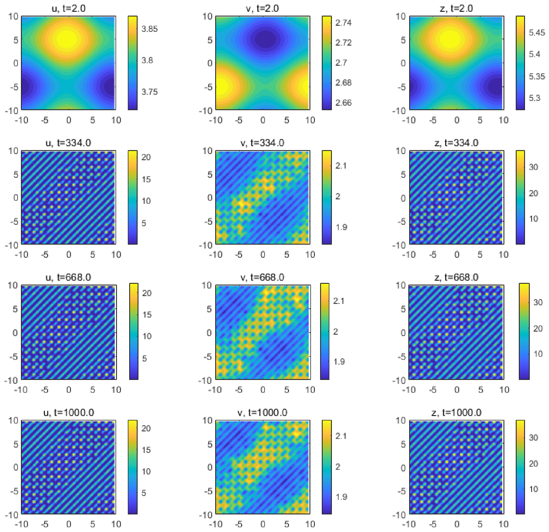
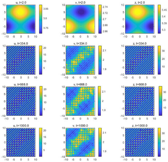
For $R=3$, the three fields have a striped configuration at $t=1000$ (Figure 1). With this shorter averaging range, the population responds mainly to nearby toxin information and forms elongated regions of high and low density. This interpretation is limited to the simulated fields and does not show that stripes improve survival.

Figure 1. Population density (u, left), toxin concentration (v, middle), and cognitive information (z, right) for system (1) at $t=1000$, with perceptual range $R=3$ and the remaining parameters as in (79). The displayed fields have a striped configuration.

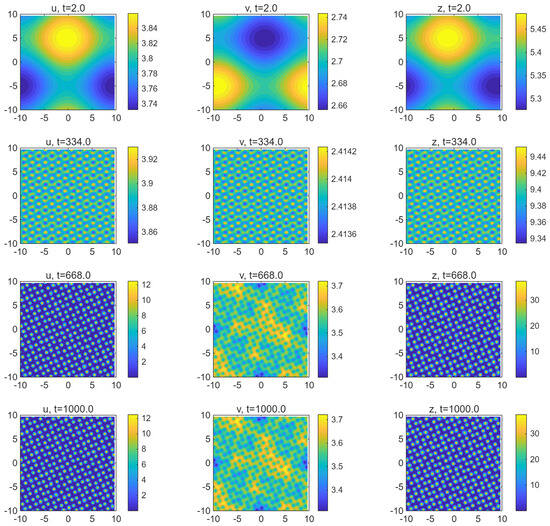
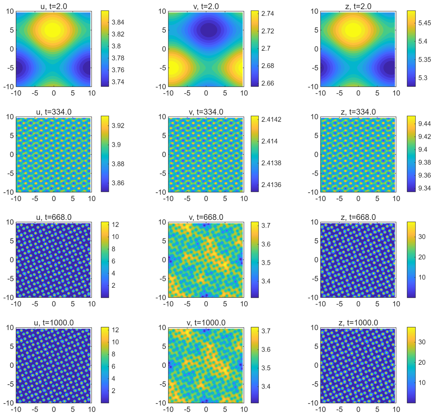
For $R=6$, with all other parameters and initial data unchanged, the fields have a spotted configuration at $t=1000$ (Figure 2). The wider kernel incorporates information from a larger neighborhood, and the simulated population is concentrated in separated patches. This comparison shows a change in spatial organization for the chosen parameter set, but it does not establish greater persistence or stability of the spotted state.

Figure 2. Population density (u, left), toxin concentration (v, middle), and cognitive information (z, right) for system (1) at $t=1000$, with perceptual range $R=6$ and the remaining parameters as in (79). The displayed fields have a spotted configuration.

A possible interpretation is a lake with localized contamination, where animals use recent or socially transmitted information to avoid polluted regions. The simulations suggest that the spatial scale of this information may affect whether high-density regions form corridors or isolated patches. Testing this interpretation would require field estimates of R, b, and $\gamma$, together with observations linking the predicted patterns to exposure or demographic outcomes.

6. Conclusions

The model couples a population and an environmental toxin to an information field generated by their local encounters. A convolution of this field drives nonlocal avoidance. On the two-dimensional torus, the system is locally well posed and admits a global uniformly bounded solution. Under the stated sufficient conditions, solutions converge exponentially to either the positive equilibrium or the toxin-only equilibrium.

With all other parameters fixed, increasing the perceptual radius from $R=3$ to $R=6$ changes the computed pattern from stripes to spots. This result concerns spatial organization in the model. It does not demonstrate improved persistence, biodiversity, or management effectiveness, and the lake scenario remains an interpretation to be tested empirically.

The information variable and its parameters have not been calibrated against movement or exposure data. Further work could estimate perceptual and memory scales, test the predicted spatial transition, and consider heterogeneous domains, time-dependent kernels, or multispecies interactions [37].

References

1. Dell’Omo, G. (Ed.) Behavioural Ecotoxicology; John Wiley & Sons: Chichester, UK, 2002. [Google Scholar]
2. Huang, Q.; Wang, H.; Lewis, M.A. The impact of environmental toxins on predator–prey dynamics. J. Theor. Biol. 2015, 378, 12–30. [Google Scholar] [CrossRef] [Scilit] [PubMed]
3. Kooijman, S.; Bedaux, J.J. The Analysis of Aquatic Toxicity Data; VU University Press: Amsterdam, The Netherlands, 1996. [Google Scholar]
4. Pastorok, R.A.; Bartell, S.M.; Ferson, S.; Ginzburg, L.R. Ecological Modeling in Risk Assessment: Chemical Effects on Populations, Ecosystems, and Landscapes; CRC Press: Boca Raton, FL, USA, 2016. [Google Scholar]
5. Scott, G.R.; Sloman, K.A. The effects of environmental pollutants on complex fish behaviour: Integrating behavioural and physiological indicators of toxicity. Aquat. Toxicol. 2004, 68, 369–392. [Google Scholar] [CrossRef] [Scilit] [PubMed]
6. Wang, J.; Shi, J.; Wei, J. Dynamics and pattern formation in a diffusive predator–prey system with strong Allee effect in prey. J. Differ. Equ. 2011, 251, 1276–1304. [Google Scholar] [CrossRef] [Scilit]
7. Winkler, M. Aggregation vs. global diffusive behavior in the higher-dimensional Keller–Segel model. J. Differ. Equ. 2010, 248, 2889–2905. [Google Scholar] [CrossRef] [Scilit]
8. Wu, J. Theory and Applications of Partial Functional Differential Equations; Springer: Berlin/Heidelberg, Germany, 1996. [Google Scholar]
9. Zhang, X.; Li, S.; Yuan, Y.; An, Q. Effect of Discontinuous Harvesting on a Diffusive Predator-Prey Model. Nonlinearity 2024, 37, 115016. [Google Scholar] [CrossRef] [Scilit]
10. Dugatkin, L.A. Principles of Animal Behavior; University of Chicago Press: Chicago, IL, USA, 2020. [Google Scholar]
11. Stephens, D.W.; Krebs, J.R. Foraging Theory; Princeton University Press: Princeton, NJ, USA, 1986; Volume 6. [Google Scholar]
12. Stevens, M. Sensory Ecology, Behaviour, and Evolution; Oxford University Press: Oxford, UK, 2013. [Google Scholar]
13. Tierney, K.B. Chemical avoidance responses of fishes. Aquat. Toxicol. 2016, 174, 228–241. [Google Scholar] [CrossRef] [Scilit] [PubMed]
14. Zhang, X.; Wu, B. Dynamics of a Diffusion-Advection Model with Local Perception of Toxins. Chaos Solitons Fractals 2025, 201, 117259. [Google Scholar] [CrossRef] [Scilit]
15. Zhang, X.; An, Q.; Wang, H. Global Solvability and Stability of Cognitive Consumer-Resource Model with Nonlocal Usage of Memory. J. Math. Anal. Appl. 2026, 556, 130076. [Google Scholar] [CrossRef] [Scilit]
16. Wang, H.; Salmaniw, Y. Open Problems in PDE Models for Knowledge-Based Animal Movement via Nonlocal Perception and Cognitive Mapping. J. Math. Biol. 2023, 86, 71. [Google Scholar] [CrossRef] [Scilit] [PubMed]
17. Shan, C.; Huang, Q. Direct and indirect effects of toxins on competition dynamics of species in an aquatic environment. J. Math. Biol. 2019, 78, 739–766. [Google Scholar] [PubMed]
18. Deng, X.; Huang, Q.; Wang, Z.A. Global Dynamics and Pattern Formation in a Diffusive Population-Toxicant Model with Negative Toxicant-Taxis. SIAM J. Appl. Math. 2023, 83, 2212–2236. [Google Scholar] [CrossRef] [Scilit]
19. Xing, J.; Huang, Q.; Nie, H. Dynamical Analysis of a Diffusive Population-Toxicant Model with Toxicant-Taxis in Polluted Aquatic Environments. Math. Biosci. 2024, 372, 109193. [Google Scholar] [CrossRef] [Scilit] [PubMed]
20. Bellomo, N.; Bellouquid, A.; Tao, Y.; Winkler, M. Toward a Mathematical Theory of Keller–Segel Models of Pattern Formation in Biological Tissues. Math. Model. Methods Appl. Sci. 2015, 25, 1663–1763. [Google Scholar] [CrossRef] [Scilit]
21. Xu, T.; Ji, S.; Mei, M.; Yin, J. On a Chemotaxis Model with Degenerate Diffusion: Initial Shrinking, Eventual Smoothness and Expanding. J. Differ. Equ. 2020, 268, 414–446. [Google Scholar] [CrossRef] [Scilit]
22. Potts, J.R.; Lewis, M.A. Spatial Memory and Taxis-Driven Pattern Formation in Model Ecosystems. Bull. Math. Biol. 2019, 81, 2725–2747. [Google Scholar] [CrossRef] [Scilit] [PubMed]
23. Painter, K.J.; Hillen, T.; Potts, J.R. Biological Modeling with Nonlocal Advection–Diffusion Equations. Math. Model. Methods Appl. Sci. 2024, 34, 57–107. [Google Scholar] [CrossRef] [Scilit]
24. Song, Y.; Wang, H.; Wang, J. Cognitive Consumer-Resource Spatiotemporal Dynamics with Nonlocal Perception. J. Nonlinear Sci. 2024, 34, 19. [Google Scholar] [CrossRef] [Scilit]
25. Xue, S.; Song, Y.; Wang, H. Spatio-Temporal Dynamics in a Reaction-Diffusion Equation with Nonlocal Spatial Memory. SIAM J. Appl. Dyn. Syst. 2024, 23, 641–667. [Google Scholar] [CrossRef] [Scilit]
26. Bo, X.; Chu, C.; Liu, W.; Lv, G.; Zhang, X. Bifurcation and stability analysis of cognitive populations in toxic environments. Commun. Nonlinear Sci. Numer. Simul. 2025, 144, 108674. [Google Scholar] [CrossRef] [Scilit]
27. Berdahl, A.; Torney, C.J.; Ioannou, C.C.; Faria, J.J.; Couzin, I.D. Emergent sensing of complex environments by mobile animal groups. Science 2013, 339, 574–576. [Google Scholar] [CrossRef] [Scilit] [PubMed]
28. Bracis, C.; Gurarie, E.; Van Moorter, B.; Goodwin, R.A. Memory effects on movement behavior in animal foraging. PLoS ONE 2015, 10, e0136057. [Google Scholar] [CrossRef] [Scilit] [PubMed]
29. Couzin, I.D. Collective cognition in animal groups. Trends Cogn. Sci. 2009, 13, 36–43. [Google Scholar] [CrossRef] [Scilit] [PubMed]
30. Mogilner, A.; Edelstein-Keshet, L. A non-local model for a swarm. J. Math. Biol. 1999, 38, 534–570. [Google Scholar] [CrossRef] [Scilit]
31. Carrillo, J.A.; Salmaniw, Y.; Skrzeczkowski, J. Well-Posedness of Aggregation-Diffusion Systems with Irregular Kernels. arXiv 2024, arXiv:2406.09227. [Google Scholar]
32. Giunta, V.; Hillen, T.; Lewis, M.A.; Potts, J. Detecting minimum energy states and multi-stability in nonlocal advection-diffusion models for interacting species. J. Math. Biol. 2022, 85, 56. [Google Scholar] [CrossRef] [Scilit] [PubMed]
33. Amann, H. Dynamic theory of quasilinear parabolic equations. II. Reaction-diffusion systems. Differ. Integral Equ. 1990, 3, 13–75. [Google Scholar] [CrossRef] [Scilit]
34. Ladyzhenskaia, O.A.; Solonnikov, V.A.; Ural’tseva, N.N. Linear and Quasi-Linear Equations of Parabolic Type; American Mathematical Soc.: Providence, RI, USA, 1968; Volume 23. [Google Scholar]
35. Farkas, B.; Wegner, S.A. Variations on Barbălat’s lemma. Am. Math. Mon. 2016, 123, 825–830. [Google Scholar] [CrossRef] [Scilit]
36. Tao, Y.; Winkler, M. Large Time Behavior in a Multidimensional Chemotaxis-Haptotaxis Model with Slow Signal Diffusion. SIAM J. Math. Anal. 2015, 47, 4229–4250. [Google Scholar] [CrossRef] [Scilit]
37. Potts, J.; Giunta, V.; Lewis, M.A. Beyond resource selection: Emergent spatio-temporal distributions from animal movements and stigmergent interactions. Oikos 2022, 2022, e09188. [Google Scholar] [CrossRef] [Scilit]
Disclaimer/Publisher’s Note: The statements, opinions and data contained in all publications are solely those of the individual author(s) and contributor(s) and not of MDPI and/or the editor(s). MDPI and/or the editor(s) disclaim responsibility for any injury to people or property resulting from any ideas, methods, instructions or products referred to in the content.
Article Metrics
Citations
Article Access Statistics
Multiple requests from the same IP address are counted as one view.