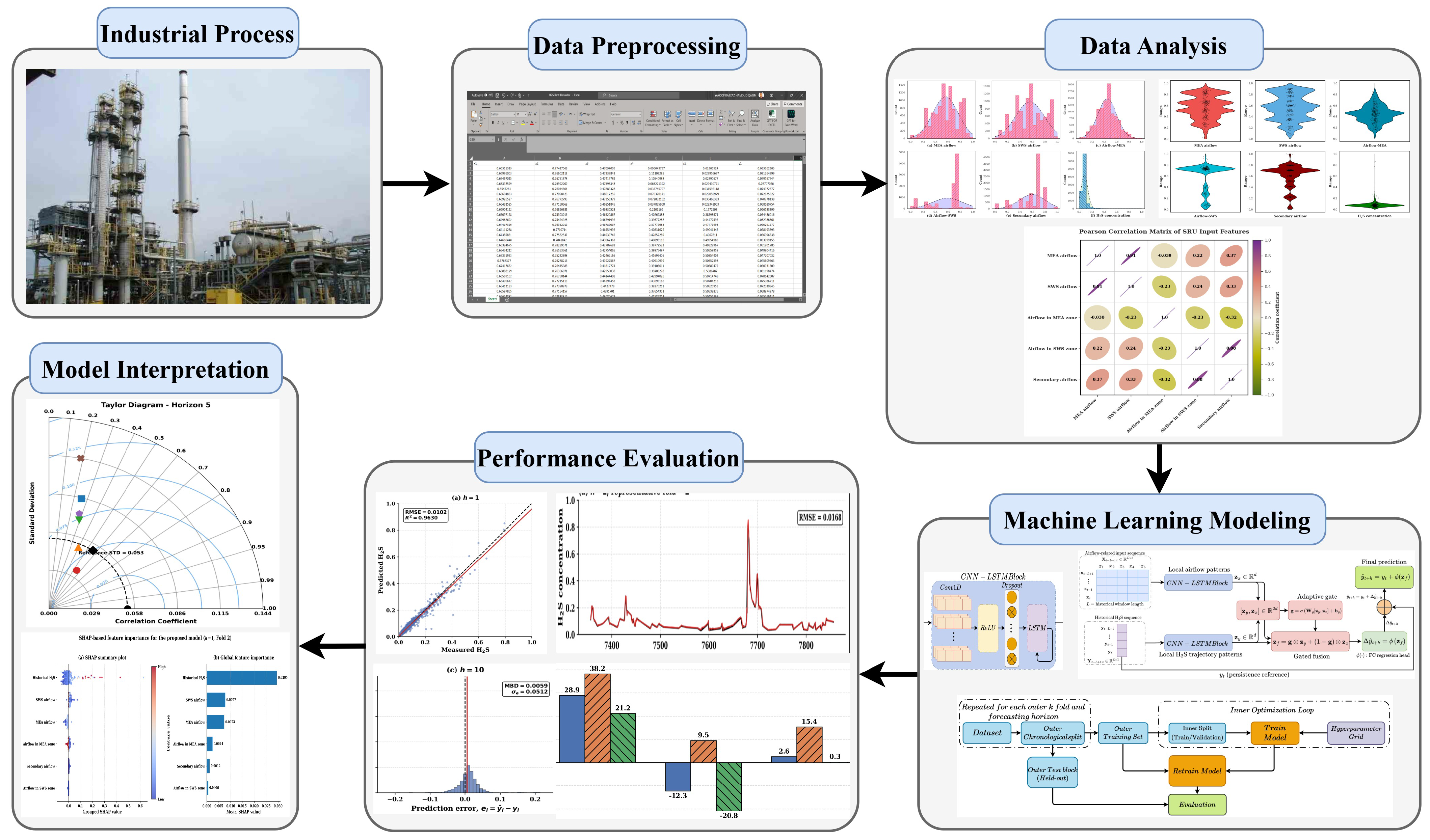
A Residual Exogenous–Autoregressive Gated Forecasting Framework for Nonlinear Dynamic Time Series: Application to Hydrogen Sulfide Prediction


Abstract
1. Introduction
- A residual exogenous–autoregressive forecasting formulation is proposed for persistent nonlinear dynamic time series, where the future target value is modeled as a persistence reference plus a learnable nonlinear correction.
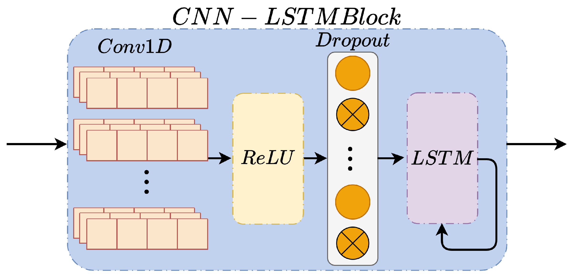
- A dual-branch CNN-LSTM architecture is developed to separately encode historical H2S dynamics and exogenous airflow dynamics, allowing autoregressive and process-input information to be represented in distinct latent spaces.
- A sample-dependent sigmoid gating mechanism is introduced to adaptively fuse autoregressive and exogenous latent representations before residual prediction.
- A leakage-aware nested blocked evaluation protocol is used to compare the proposed framework with persistence, tree-based ARX models, recurrent models, convolutional recurrent models, and compact Transformer-family baselines.
- A comprehensive evaluation is conducted using predictive metrics, computational complexity, inference latency, Taylor diagrams, and horizon-wise SHAP analysis to assess forecasting accuracy, deployment feasibility, and physical interpretability.
2. Mathematical Formulation and Methodology
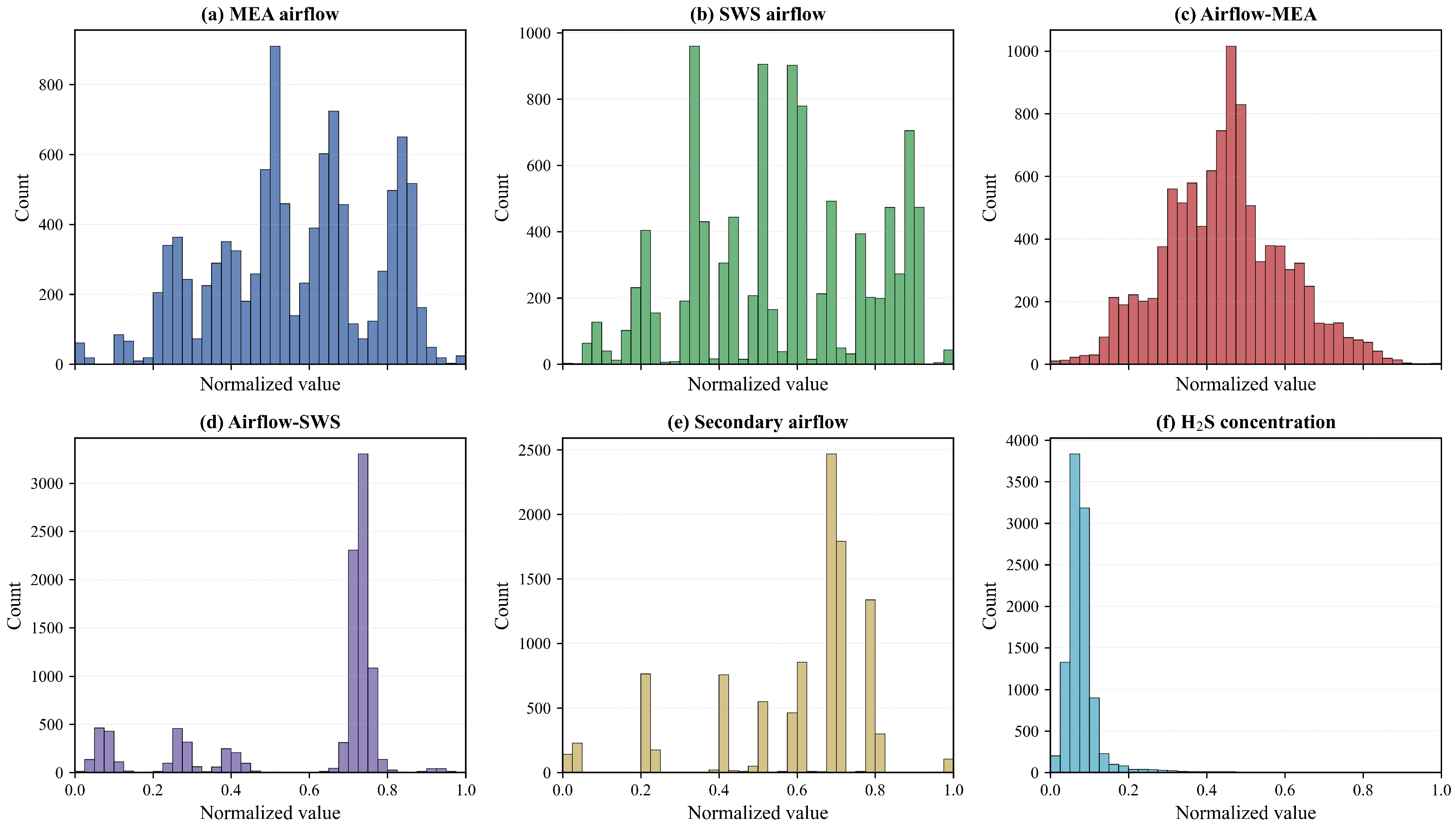
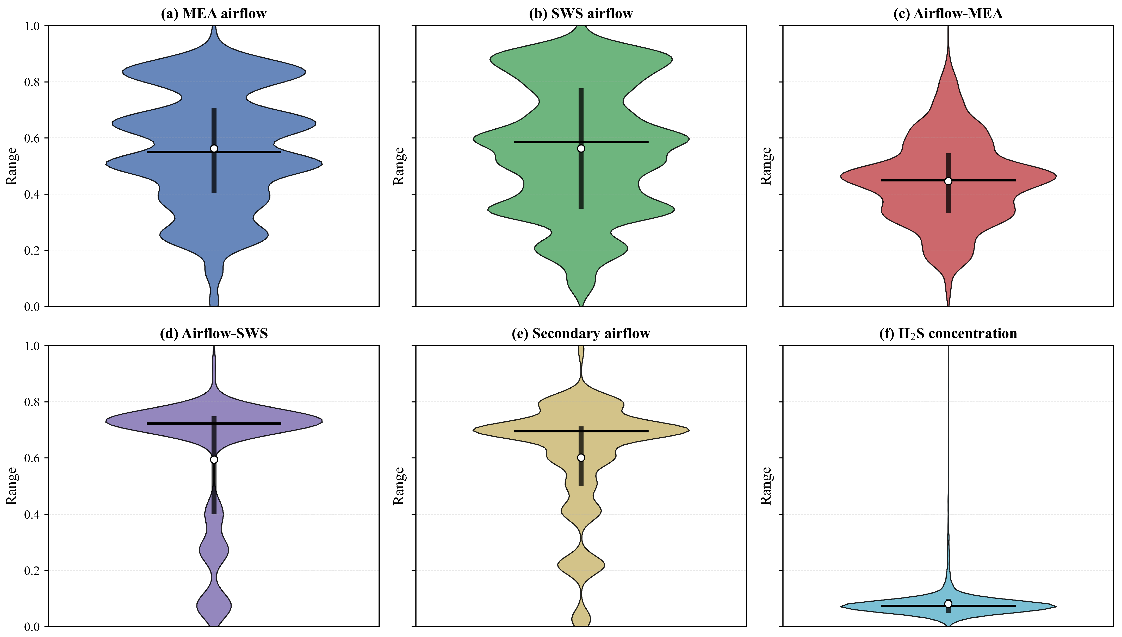
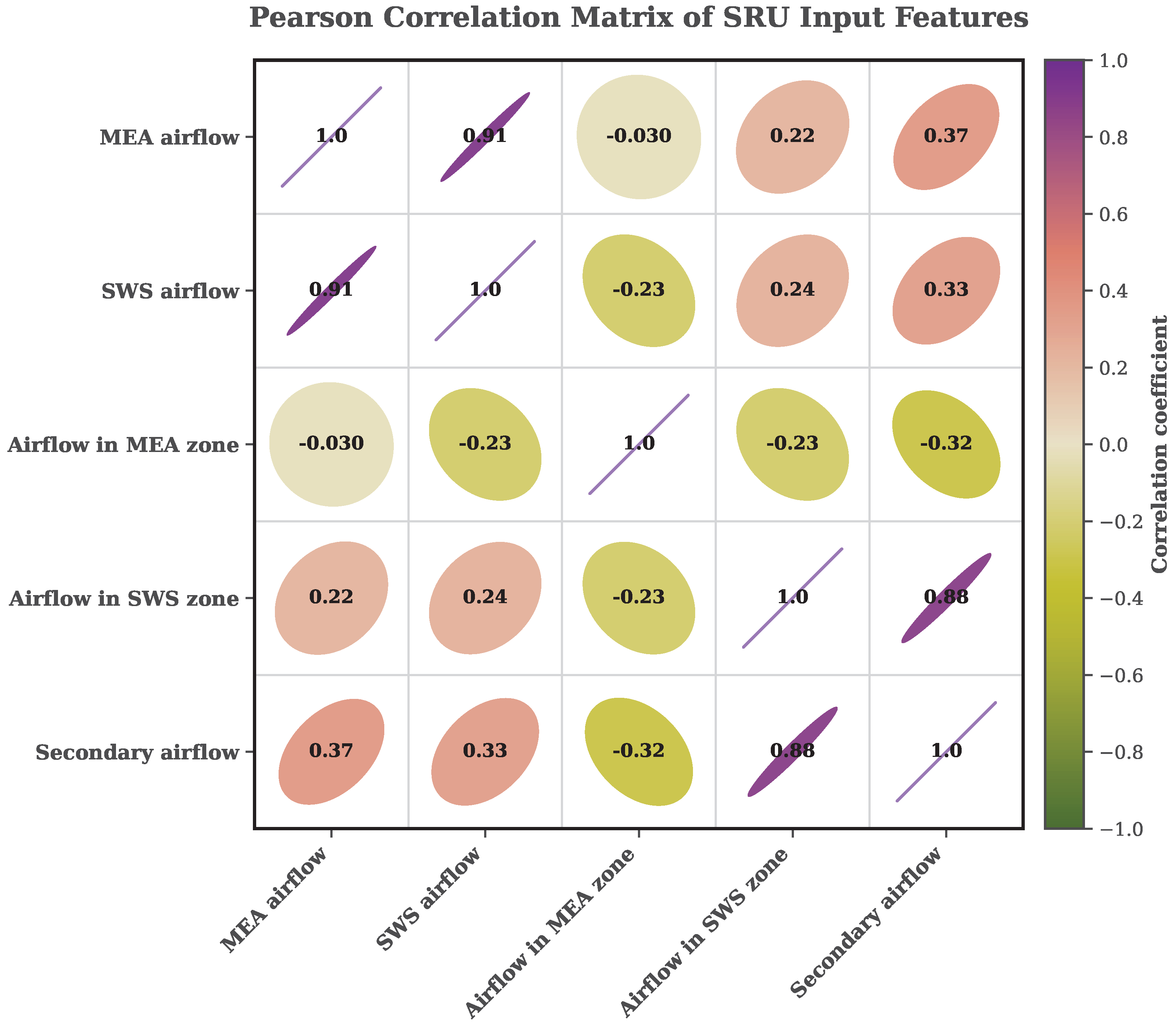
2.1. Dataset Description and Analysis
2.2. Multi-Horizon Exogenous–Autoregressive Forecasting Problem
2.3. Residual Exogenous–Autoregressive Decomposition
2.4. Data Preprocessing and Sequence Construction
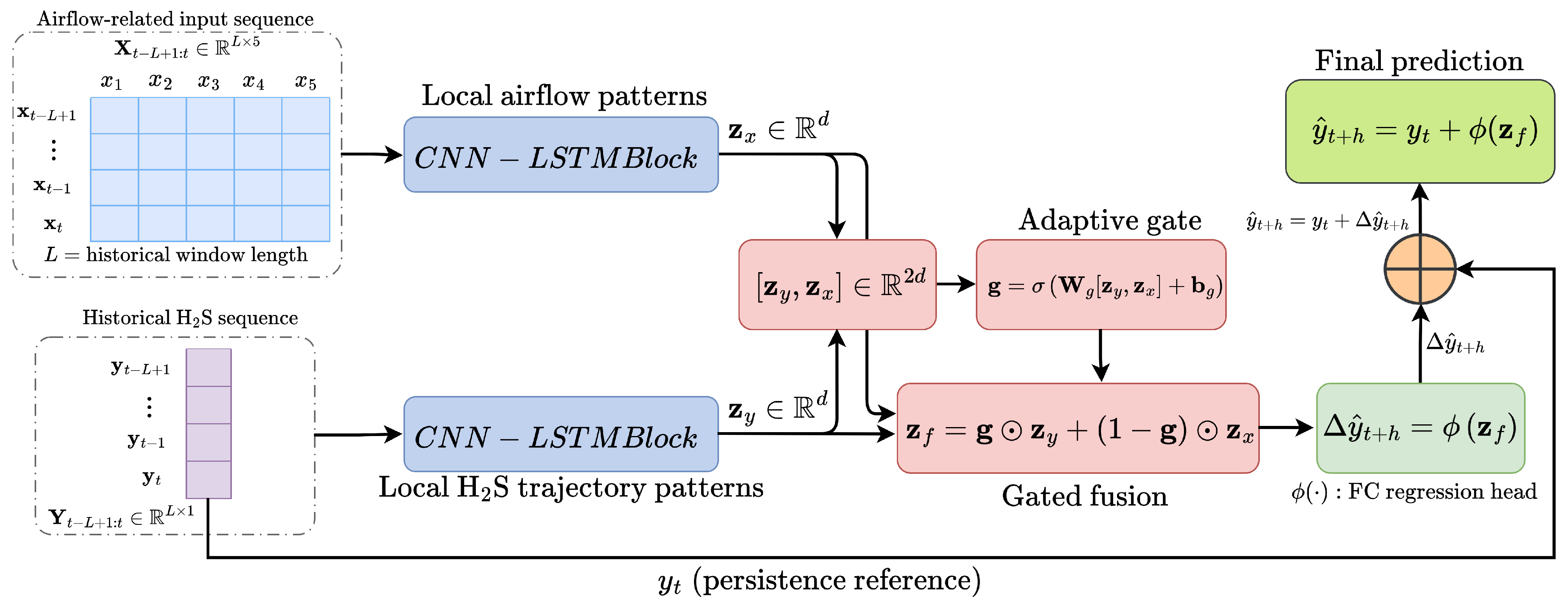
2.5. Proposed Residual Gated Forecasting Framework
2.6. Optimization Objective and Training Procedure
| Algorithm 1: Training and prediction procedure of the proposed residual gated forecasting framework |
| Require: Exogenous sequence , autoregressive target sequence , latest target value , target value Ensure: Predicted target value
|
2.7. Baseline Models
2.8. Hyperparameter Optimization and Experimental Protocol
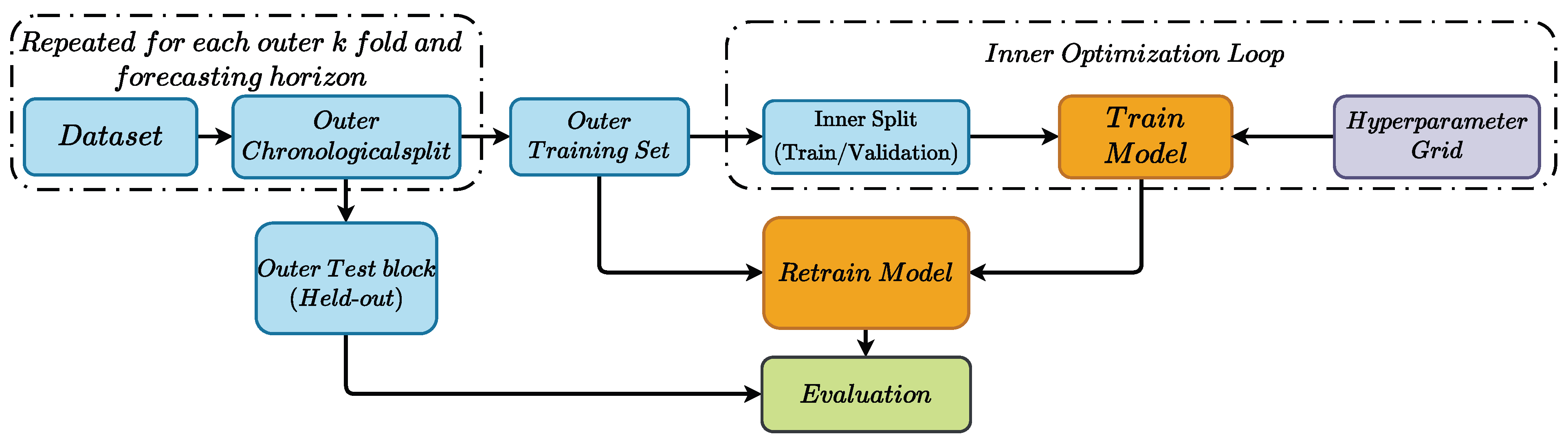
- Construct the supervised forecasting dataset for each horizon .
- Split the ordered dataset into chronological outer training and test blocks.
- Split each outer training block into inner training and inner validation subsets.
- Train each candidate hyperparameter configuration on the inner training subset.
- Select the best configuration using the inner validation RMSE.
- Retrain the selected configuration on the full outer training subset.
- Evaluate the retrained model once on the held-out outer test subset.
- Repeat the procedure for all outer folds, forecasting horizons, and evaluated models.
2.9. Evaluation Metrics
3. Results and Discussion
3.1. Overall Predictive Performance
3.2. Improvement over the Persistence Baseline
3.3. Computational Complexity and Runtime Analysis
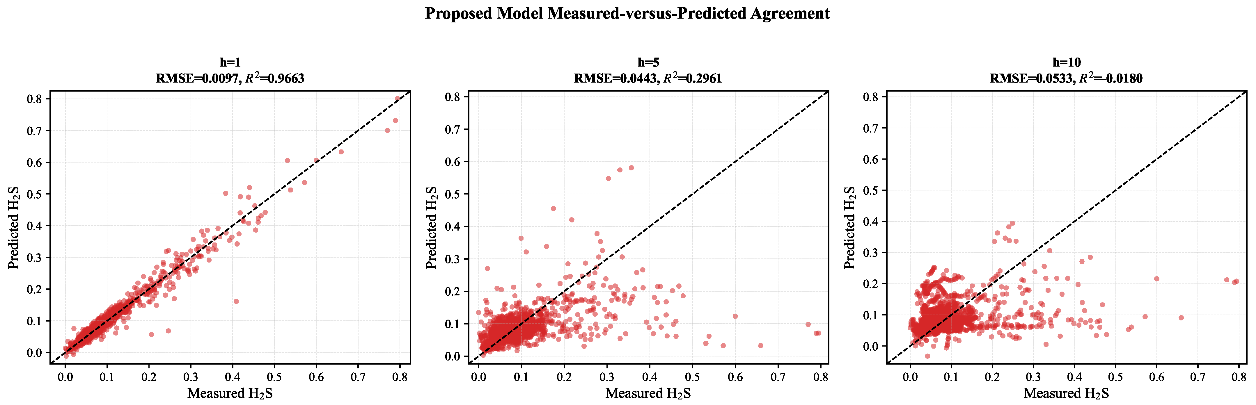
3.4. Dynamic Tracking and Regression Agreement of the Proposed Model
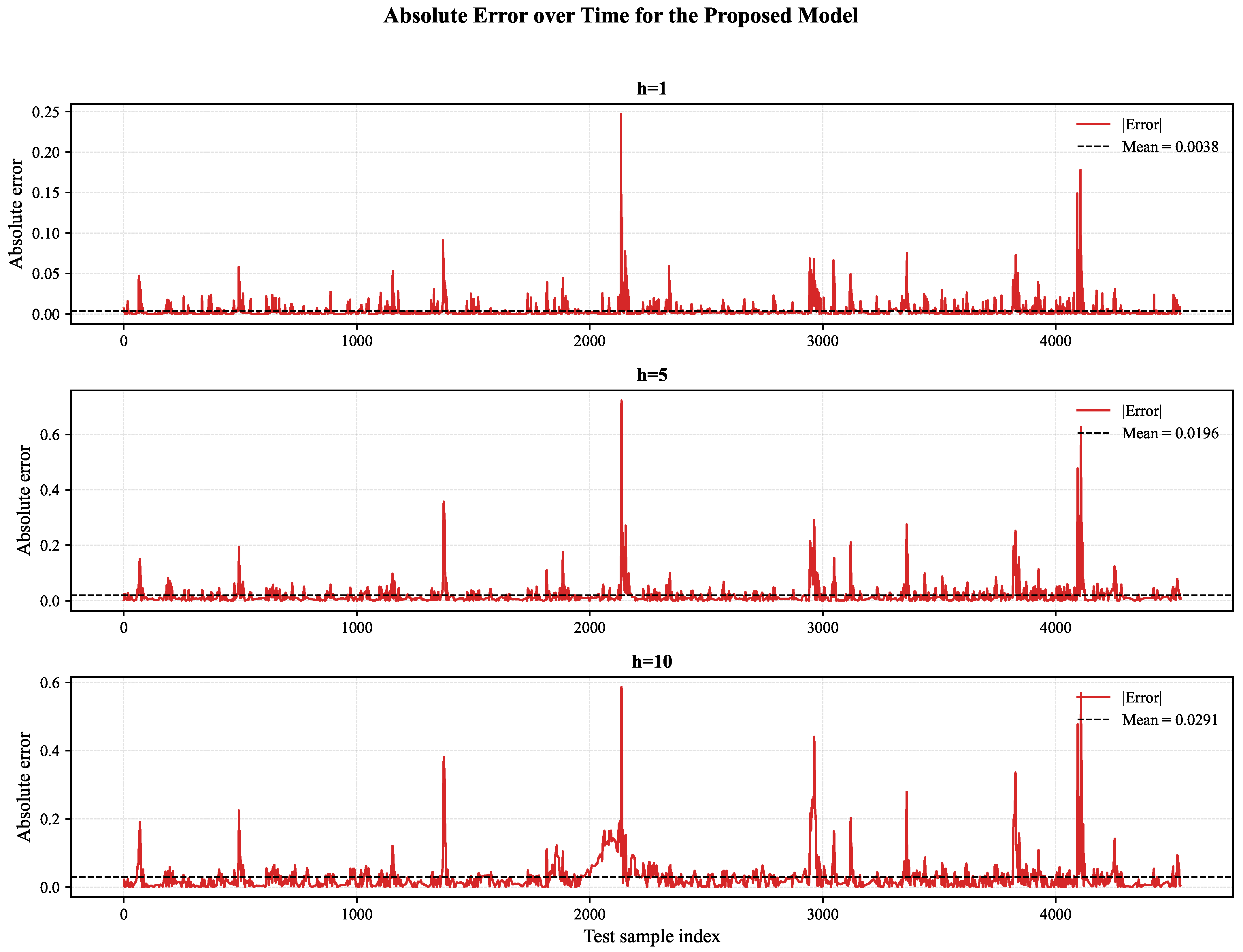
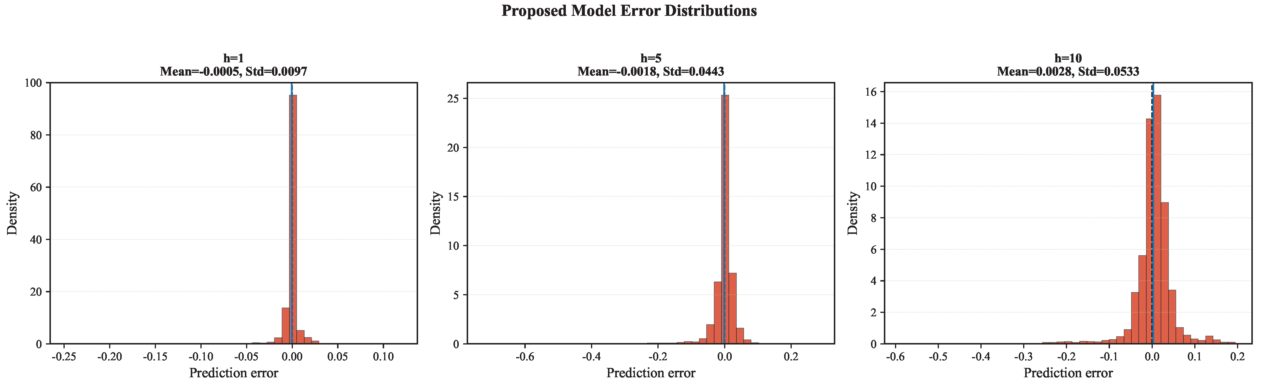
3.5. Prediction Error Distribution and Absolute Error Analysis
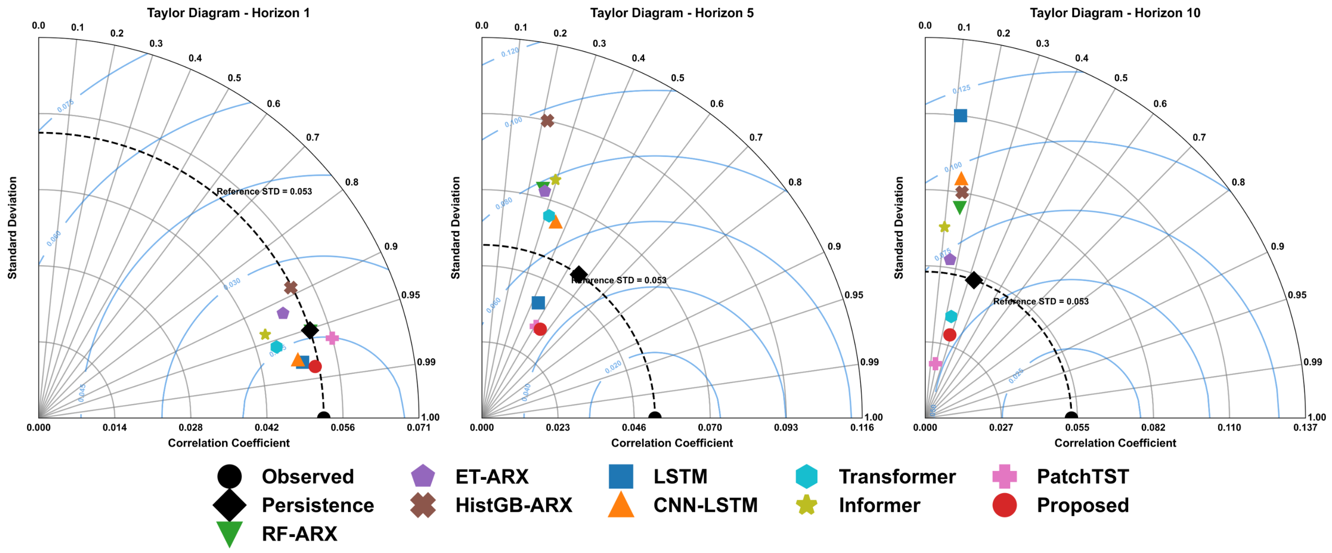
3.6. Taylor Diagram Analysis
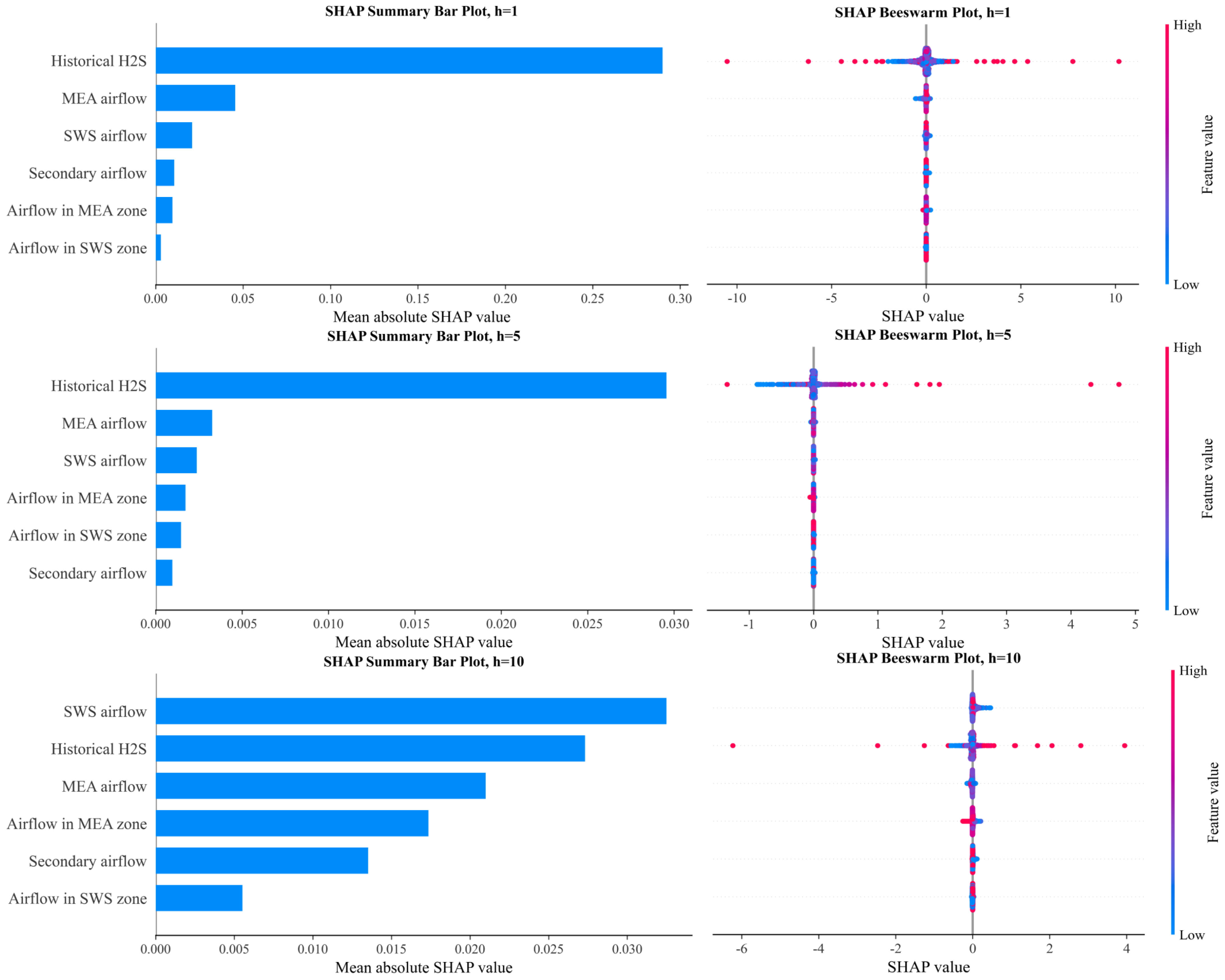
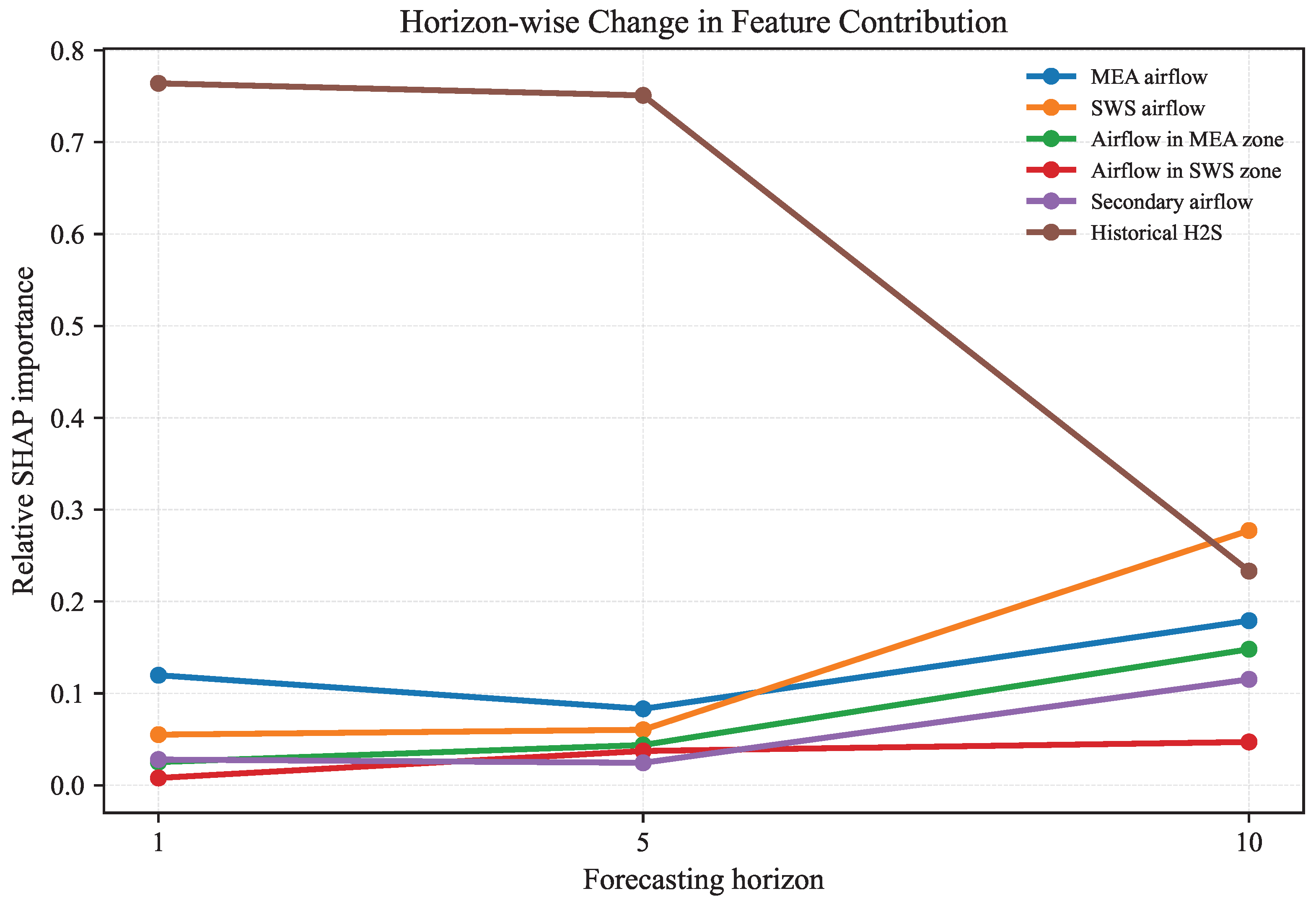
3.7. SHAP-Based Horizon-Wise Interpretability Analysis
3.8. Practical Implications, Generalizability, and Limitations
4. Conclusions
Funding
Data Availability Statement
Conflicts of Interest
References
- Fortuna, L.; Graziani, S.; Rizzo, A.; Xibilia, M.G. Soft Sensors for Monitoring and Control of Industrial Processes; Springer: London, UK, 2007. [Google Scholar]
- Kadlec, P.; Gabrys, B.; Strandt, S. Data-driven soft sensors in the process industry. Comput. Chem. Eng. 2009, 33, 795–814. [Google Scholar] [CrossRef]
- Perera, Y.S.; Ratnaweera, D.A.A.C.; Dasanayaka, C.H.; Abeykoon, C. The role of artificial intelligence-driven soft sensors in advanced sustainable process industries: A critical review. Eng. Appl. Artif. Intell. 2023, 121, 105988. [Google Scholar] [CrossRef]
- Cao, L.; Wang, J.; Su, J.; Luo, Y.; Cao, Y.; Braatz, R.D.; Gopaluni, B. Comprehensive analysis on machine learning approaches for interpretable and stable soft sensors. IEEE Trans. Instrum. Meas. 2025, 74, 9517217. [Google Scholar] [CrossRef]
- Pudi, A.; Rezaei, M.; Signorini, V.; Andersson, M.P.; Baschetti, M.G.; Mansouri, S.S. Hydrogen sulfide capture and removal technologies: A comprehensive review of recent developments and emerging trends. Sep. Purif. Technol. 2022, 298, 121448. [Google Scholar] [CrossRef]
- Chan, Y.H.; Loy, A.C.M.; Cheah, K.W.; Chai, S.Y.W.; Ngu, L.H.; How, B.S.; Li, C.; Lock, S.S.M.; Wong, M.K.; Yiin, C.L.; et al. Hydrogen sulfide (H2S) conversion to hydrogen (H2) and value-added chemicals: Progress, challenges and outlook. Chem. Eng. J. 2023, 458, 141398. [Google Scholar] [CrossRef]
- Zhang, X.; Tang, Y.; Qu, S.; Da, J.; Hao, Z. H2S-Selective Catalytic Oxidation: Catalysts and Processes. ACS Catal. 2015, 5, 1053–1067. [Google Scholar] [CrossRef]
- Manenti, F.; Papasidero, D.; Bozzano, G.; Ranzi, E. Model-based optimization of sulfur recovery units. Comput. Chem. Eng. 2014, 66, 244–251. [Google Scholar] [CrossRef]
- Kazempour, H.; Pourfayaz, F.; Mehrpooya, M. Modeling and multi-optimization of thermal section of Claus process based on kinetic model. J. Nat. Gas. Sci. Eng. 2017, 38, 235–244. [Google Scholar] [CrossRef]
- Ghahraloud, H.; Farsi, M.; Rahimpour, M. Modeling and optimization of an industrial Claus process: Thermal and catalytic section. J. Taiwan Inst. Chem. Eng. 2017, 76, 1–9. [Google Scholar] [CrossRef]
- Rahman, R.K.; Ibrahim, S.; Raj, A. Multi-objective optimization of sulfur recovery units using a detailed reaction mechanism to reduce energy consumption and destruct feed contaminants. Comput. Chem. Eng. 2019, 128, 21–34. [Google Scholar] [CrossRef]
- Duque, H.; Diao, K.; Villa, R.; Leitão, J.P.; Djordjević, S.; Abdel-Aal, M. Context-aware data driven sensor data analysis: With application to H2S concentration prediction in urban drainage networks. Water Res. X 2025, 28, 100346. [Google Scholar] [CrossRef]
- Kychkin, A.; Chernitsin, I.; Vikentyeva, O. Development the reinforcement learning model for sources identification of H2S industrial emissions. In Proceedings of the International Conference on Industrial Engineering, Applications and Manufacturing (ICIEAM), Sochi, Russia, 12–16 May 2025. [Google Scholar]
- Johni, A.K.; OmidbakhshAmiri, E. Simulation and multi-objective optimization of Claus process of sulfur recovery unit. J. Environ. Chem. Eng. 2023, 11, 110969. [Google Scholar] [CrossRef]
- Khan, I.; Saghir, H.; Ahsan, M. Machine learning-enabled prediction and optimization of sulfur recovery units: A step towards Industry 4.0 integration. Mater. Proc. 2024, 17, 6. [Google Scholar] [CrossRef]
- Ge, Z.; Song, Z. Nonlinear soft sensor development based on relevance vector machine. Ind. Eng. Chem. Res. 2010, 49, 8685–8693. [Google Scholar] [CrossRef]
- Bidar, B.; Shahraki, F.; Sadeghi, J.; Khalilipour, M.M. Soft sensor modeling based on multi-state-dependent parameter models and application for quality monitoring in industrial sulfur recovery process. IEEE Sens. J. 2018, 18, 4583–4591. [Google Scholar] [CrossRef]
- Tavakoli Dastjerd, F.; Shahraki, F.; Sadeghi, J.; Khalilipour, M.M.; Bidar, B. Tail gas quality warning system in a sulfur recovery unit based on. Int. J. Ind. Electron. Control Optim. 2023, 6, 307–319. [Google Scholar] [CrossRef]
- LeCun, Y.; Bengio, Y.; Hinton, G. Deep learning. Nature 2015, 521, 436–444. [Google Scholar] [CrossRef] [PubMed]
- Hochreiter, S.; Schmidhuber, J. Long short-term memory. Neural Comput. 1997, 9, 1735–1780. [Google Scholar] [CrossRef] [PubMed]
- Yuan, X.; Li, L.; Wang, Y. Nonlinear dynamic soft sensor modeling with supervised long short-term memory network. IEEE Trans. Ind. Inform. 2020, 16, 3168–3176. [Google Scholar] [CrossRef]
- Zhang, T.; Song, S.; Li, S.; Ma, L.; Pan, S.; Han, L. Research on gas concentration prediction models based on LSTM multidimensional time series. Energies 2019, 12, 161. [Google Scholar] [CrossRef]
- Recio-Colmenares, R.; León Becerril, E.; Gurubel Tun, K.J.; Conchas, R.F. Design of a soft sensor based on long short-term memory artificial neural network (LSTM) for wastewater treatment plants. Sensors 2023, 23, 9236. [Google Scholar] [CrossRef] [PubMed]
- Yuan, X.; Li, L.; Wang, Y.; Yang, C.; Gui, W. Deep learning for quality prediction of nonlinear dynamic processes with variable attention-based long short-term memory network. Can. J. Chem. Eng. 2020, 98, 1377–1389. [Google Scholar]
- Shen, F.; Zheng, J.; Ye, L.; Ma, X. LSTM soft sensor development of batch processes with multivariate trajectory based ensemble just-in-time learning. IEEE Access 2020, 8, 73855–73864. [Google Scholar] [CrossRef]
- Zheng, J.; Ma, L.; Wu, Y.; Ye, L.; Shen, F. Nonlinear dynamic soft sensor development with a supervised hybrid CNN-LSTM network for industrial processes. ACS Omega 2022, 7, 16653–16664. [Google Scholar] [CrossRef] [PubMed]
- Zha, W.; Liu, Y.; Wan, Y.; Luo, R.; Li, D.; Yang, S.; Xu, Y. Forecasting monthly gas field production based on the CNN-LSTM model. Energy 2022, 260, 124889. [Google Scholar] [CrossRef]
- Junior, J.S.S.; Mendes, J.; Souza, F.; Premebida, C. Hybrid LSTM-fuzzy system to model a sulfur recovery unit. In Proceedings of the 20th International Conference on Informatics in Control, Automation and Robotics; SciTePress: Rome, Italy, 2023; Volume 2, pp. 281–288. [Google Scholar] [CrossRef]
- Sun, W.; Li, L.; Lu, B.; Jiang, L.; Zhang, J. Hybrid multiscale forecasting of SRU sulfur gas concentrations using VMD, CEEMDAN and optimized PatchTST. iScience 2026, 29, 114986. [Google Scholar] [CrossRef] [PubMed]
- Dragomiretskiy, K.; Zosso, D. Variational mode decomposition. IEEE Trans. Signal Process. 2014, 62, 531–544. [Google Scholar] [CrossRef]
- Torres, M.E.; Colominas, M.A.; Schlotthauer, G.; Flandrin, P. A complete ensemble empirical mode decomposition with adaptive noise. In Proceedings of the IEEE International Conference on Acoustics, Speech and Signal Processing (ICASSP), Prague, Czech Republic, 22–27 May 2011; pp. 4144–4147. [Google Scholar]
- Vaswani, A.; Shazeer, N.; Parmar, N.; Uszkoreit, J.; Jones, L.; Gomez, A.N.; Kaiser, Ł.; Polosukhin, I. Attention is all you need. Adv. Neural Inf. Process. Syst. 2017, 30, 5998–6008. [Google Scholar]
- Nie, Y.; Nguyen, N.H.; Sinthong, P.; Kalagnanam, J. A time series is worth 64 words: Long-term forecasting with transformers. In Proceedings of the International Conference on Learning Representations (ICLR), Kigali, Rwanda, 1–5 May 2023. [Google Scholar]
- Yuan, X.; Wang, Y.; Yang, C.; Gui, W. Stacked isomorphic autoencoder based soft analyzer and its application to sulfur recovery unit. Inf. Sci. 2020, 534, 72–84. [Google Scholar] [CrossRef]
- Wang, Q.; Li, L. Research on semi-supervised soft sensor modeling method for sulfur recovery unit based on ISSA-VMD-ESN. Chem. Eng. Sci. 2024, 298, 120397. [Google Scholar] [CrossRef]
- Mou, T.; Liu, J.; Zou, Y.; Li, S.; Xibilia, M.G. Enhanced industrial process modeling with transfer-incremental-learning: A parallel SAE approach and its application to a sulfur recovery unit. Control Eng. Pract. 2024, 148, 105955. [Google Scholar] [CrossRef]
- Sun, W. Industrial Sulfur Gas Concentration Dataset for SRU Forecasting. Mendeley Data 2026, 1. [Google Scholar] [CrossRef]
- Huber, P.J. Robust estimation of a location parameter. Ann. Math. Stat. 1964, 35, 73–101. [Google Scholar] [CrossRef]
- Breiman, L. Random forests. Mach. Learn. 2001, 45, 5–32. [Google Scholar] [CrossRef]
- Geurts, P.; Ernst, D.; Wehenkel, L. Extremely randomized trees. Mach. Learn. 2006, 63, 3–42. [Google Scholar] [CrossRef]
- Friedman, J.H. Greedy function approximation: A gradient boosting machine. Ann. Stat. 2001, 29, 1189–1232. [Google Scholar] [CrossRef]
- Zhou, H.; Zhang, S.; Peng, J.; Zhang, S.; Li, J.; Xiong, H.; Zhang, W. Informer: Beyond efficient transformer for long sequence time-series forecasting. Proc. AAAI Conf. Artif. Intell. 2021, 35, 11106–11115. [Google Scholar] [CrossRef]
- Bergmeir, C.; Hyndman, R.J.; Koo, B. A note on the validity of cross-validation for evaluating autoregressive time series prediction. Comput. Stat. Data Anal. 2018, 120, 70–83. [Google Scholar] [CrossRef]
- Loshchilov, I.; Hutter, F. Decoupled weight decay regularization. In Proceedings of the International Conference on Learning Representations, New Orleans, LA, USA, 6–9 May 2019. [Google Scholar]
- Taylor, K.E. Summarizing multiple aspects of model performance in a single diagram. J. Geophys. Res. Atmos. 2001, 106, 7183–7192. [Google Scholar] [CrossRef]





| Feature | Mean | Std. Dev. | Sum | Min | Median | Max |
|---|---|---|---|---|---|---|
| MEA airflow | 0.5623 | 0.2054 | 5668.7820 | 0.0000 | 0.5502 | 1.0000 |
| SWS airflow | 0.5623 | 0.2277 | 5668.2719 | 0.0000 | 0.5857 | 1.0000 |
| Airflow in MEA zone | 0.4461 | 0.1519 | 4497.1044 | 0.0000 | 0.4494 | 1.0000 |
| Airflow in SWS zone | 0.5940 | 0.2420 | 5988.4523 | 0.0000 | 0.7225 | 1.0000 |
| Secondary airflow | 0.6011 | 0.2029 | 6059.2596 | 0.0000 | 0.6953 | 1.0000 |
| H2S concentration | 0.0807 | 0.0530 | 813.6129 | 0.0000 | 0.0734 | 1.0000 |
| Component | Input | Operation | Output |
|---|---|---|---|
| Exogenous encoder | Temporal convolution, activation, dropout, and LSTM encoding | ||
| Autoregressive encoder | Temporal convolution, activation, dropout, and LSTM encoding | ||
| Adaptive gate | Fully connected transformation followed by sigmoid activation | ||
| Gated fusion | , , and | Element-wise latent interpolation | |
| Residual head | Fully connected nonlinear regression mapping | ||
| Final prediction | and | Residual addition |
| Model | Category | Purpose of Comparison |
|---|---|---|
| Naive persistence | Reference predictor | Tests whether the proposed residual operator learns useful corrections beyond direct carry-forward prediction. |
| Random Forest-ARX | Tree-based nonlinear ARX model | Evaluates nonlinear ensemble regression using flattened historical exogenous and autoregressive features. |
| Extra Trees-ARX | Randomized tree-based ARX model | Tests whether additional randomization in tree ensembles improves nonlinear forecasting from vectorized ARX features. |
| HistGB-ARX | Boosting-based ARX model | Evaluates additive boosted-tree regression using the same flattened temporal information. |
| LSTM | Single-stream recurrent sequence model | Tests recurrent temporal modeling of the full sequence without convolution, residual prediction, or exogenous–autoregressive separation. |
| CNN-LSTM | Single-stream convolutional –recurrent model | Tests local temporal feature extraction followed by recurrent modeling without dual-branch gated residual fusion. |
| Transformer | Attention-based sequence model | Evaluates self-attention-based temporal representation of the full input sequence. |
| Informer | Compact attention-based sequence model | Evaluates an attention-based long-range dependency baseline with sequence-level aggregation. |
| PatchTST | Patch-based Transformer sequence model | Evaluates patch-level temporal tokenization and attention-based forecasting. |
| Proposed framework | Residual gated exogenous– autoregressive model | Tests whether residual prediction, dual-branch temporal encoding, and adaptive gated fusion improve multi-horizon forecasting. |
| Model Group | Hyperparameter | Candidate/Fixed Values |
|---|---|---|
| All window-based models | Window length L | |
| Random Forest-ARX | Number of trees | |
| Maximum tree depth | ||
| Minimum samples per leaf | ||
| Extra Trees-ARX | Number of trees | |
| Maximum tree depth | ||
| Minimum samples per leaf | ||
| HistGB-ARX | Learning rate | |
| Maximum leaf nodes | ||
| Maximum iterations | ||
| LSTM | LSTM hidden units | |
| LSTM layers | 1 | |
| Dropout rate | ||
| Learning rate | ||
| Batch size | ||
| CNN-LSTM | CNN filters | |
| CNN kernel size | ||
| LSTM hidden units | ||
| LSTM layers | 1 | |
| Dropout rate | ||
| Learning rate | ||
| Batch size | ||
| Transformer and Informer | Embedding dimension | |
| Number of attention heads | 2 | |
| Encoder layers | ||
| Dropout rate | ||
| Learning rate | ||
| Batch size | ||
| PatchTST | Embedding dimension | |
| Number of attention heads | 2 | |
| Encoder layers | ||
| Patch length | ||
| Patch stride | 2 | |
| Dropout rate | ||
| Learning rate | ||
| Batch size | ||
| Proposed framework | CNN filters | |
| CNN kernel size | ||
| LSTM hidden units | ||
| LSTM layers | 1 | |
| Dropout rate | ||
| Learning rate | ||
| Batch size | ||
| Training protocol | Maximum epochs | 80 |
| Early stopping patience | 12 epochs | |
| Weight decay | ||
| Gradient clipping |
| Model | |||
|---|---|---|---|
| Random Forest–ARX | ; ; depth ; leaf | ; ; depth ; leaf | ; ; depth ; leaf |
| Extra Trees–ARX | ; ; depth ; leaf | ; ; depth ; leaf | ; ; depth ; leaf |
| HistGB–ARX | ; ; leaves ; iter | ; ; leaves ; iter | ; ; leaves ; iter |
| LSTM | ; ; drop ; lr ; bs | ; ; drop ; lr ; bs | ; ; drop ; lr ; bs |
| CNN–LSTM | ; ; ; ; drop ; lr ; bs | ; ; ; ; drop ; lr ; bs | ; ; ; ; drop ; lr ; bs |
| Transformer | ; ; heads ; layers ; drop ; lr ; bs | ; ; heads ; layers ; drop ; lr ; bs | ; ; heads ; layers ; drop ; lr ; bs |
| Informer | ; ; heads ; layers ; drop ; lr ; bs | ; ; heads ; layers ; drop ; lr ; bs | ; ; heads ; layers ; drop ; lr ; bs |
| PatchTST | ; ; heads ; layers ; patch ; stride ; lr ; bs | ; ; heads ; layers ; patch ; stride ; lr ; bs | ; ; heads ; layers ; patch ; stride ; lr ; bs |
| Proposed | ; ; ; ; drop ; lr ; bs | ; ; ; ; drop ; lr ; bs | ; ; ; ; drop ; lr ; bs |
| Horizon | Model | MAE | RMSE | sMAPE (%) | MedAE | EV | MBD | r | |
|---|---|---|---|---|---|---|---|---|---|
| Proposed | |||||||||
| LSTM | |||||||||
| CNN–LSTM | |||||||||
| PatchTST | |||||||||
| Transformer | |||||||||
| Random Forest–ARX | |||||||||
| Naive persistence | |||||||||
| Informer | |||||||||
| Extra Trees–ARX | |||||||||
| HistGB–ARX | |||||||||
| Proposed | |||||||||
| PatchTST | |||||||||
| Naive persistence | |||||||||
| LSTM | |||||||||
| CNN–LSTM | |||||||||
| Transformer | |||||||||
| Extra Trees–ARX | |||||||||
| Informer | |||||||||
| Random Forest–ARX | |||||||||
| HistGB–ARX | |||||||||
| PatchTST | |||||||||
| Proposed | |||||||||
| Transformer | |||||||||
| Naive persistence | |||||||||
| Extra Trees–ARX | |||||||||
| Informer | |||||||||
| Random Forest–ARX | |||||||||
| HistGB–ARX | |||||||||
| CNN–LSTM | |||||||||
| LSTM |
| Horizon | Model | Parameters/ Trees–Nodes | Training Time (s) | Inference (ms/Sample) | Throughput (Samples/s) | Model Size (MB) |
|---|---|---|---|---|---|---|
| Naive persistence | 0 | 0.00 | 0.0000 | 0.000 | ||
| Random Forest–ARX | 250/293,678 | 43.98 | 0.0430 | 24,710 | 20.227 | |
| Extra Trees–ARX | 267/722,058 | 5.56 | 0.0443 | 22,683 | 49.646 | |
| HistGB–ARX | – | 1.78 | 0.0090 | 113,871 | 0.650 | |
| LSTM | 22,657 | 17.43 | 0.0276 | 36,582 | 0.089 | |
| CNN–LSTM | 28,582 | 42.34 | 0.0250 | 40,526 | 0.112 | |
| Transformer | 52,780 | 35.83 | 0.0270 | 36,993 | 0.294 | |
| Informer | 18,721 | 29.74 | 0.0269 | 37,237 | 0.143 | |
| PatchTST | 75,948 | 60.05 | 0.0250 | 40,129 | 0.300 | |
| Proposed | 51,073 | 34.88 | 0.0279 | 36,045 | 0.200 | |
| Naive persistence | 0 | 0.00 | 0.0000 | 0.000 | ||
| Random Forest–ARX | 233/366,967 | 49.42 | 0.0654 | 16,254 | 25.255 | |
| Extra Trees–ARX | 250/393,989 | 7.03 | 0.0476 | 21,063 | 27.114 | |
| HistGB–ARX | – | 2.54 | 0.0148 | 82,291 | 0.687 | |
| LSTM | 11,692 | 10.66 | 0.0246 | 41,293 | 0.047 | |
| CNN–LSTM | 7985 | 7.94 | 0.0292 | 34,702 | 0.034 | |
| Transformer | 57,878 | 29.18 | 0.0299 | 34,204 | 0.331 | |
| Informer | 49,249 | 19.82 | 0.0364 | 28,009 | 0.299 | |
| PatchTST | 45,718 | 25.70 | 0.0247 | 40,732 | 0.183 | |
| Proposed | 35,713 | 3.69 | 0.0296 | 34,630 | 0.142 | |
| Naive persistence | 0 | 0.00 | 0.0000 | 0.000 | ||
| Random Forest–ARX | 267/248,079 | 48.03 | 0.0466 | 21,494 | 17.099 | |
| Extra Trees–ARX | 250/964,311 | 5.69 | 0.0453 | 22,377 | 66.276 | |
| HistGB–ARX | – | 1.95 | 0.0117 | 95,482 | 0.591 | |
| LSTM | 6209 | 11.44 | 0.0250 | 40,606 | 0.026 | |
| CNN–LSTM | 28,582 | 5.69 | 0.0232 | 43,638 | 0.112 | |
| Transformer | 88,108 | 10.59 | 0.0247 | 41,061 | 0.468 | |
| Informer | 18,721 | 17.73 | 0.0260 | 38,690 | 0.143 | |
| PatchTST | 75,948 | 20.58 | 0.0311 | 34,297 | 0.300 | |
| Proposed | 52,609 | 9.13 | 0.0343 | 29,921 | 0.206 |
Disclaimer/Publisher’s Note: The statements, opinions and data contained in all publications are solely those of the individual author(s) and contributor(s) and not of MDPI and/or the editor(s). MDPI and/or the editor(s) disclaim responsibility for any injury to people or property resulting from any ideas, methods, instructions or products referred to in the content. |
© 2026 by the author. Licensee MDPI, Basel, Switzerland. This article is an open access article distributed under the terms and conditions of the Creative Commons Attribution (CC BY) license.
Share and Cite
Alghamdi, M.M. A Residual Exogenous–Autoregressive Gated Forecasting Framework for Nonlinear Dynamic Time Series: Application to Hydrogen Sulfide Prediction. Mathematics 2026, 14, 2878. https://doi.org/10.3390/math14162878
Alghamdi MM. A Residual Exogenous–Autoregressive Gated Forecasting Framework for Nonlinear Dynamic Time Series: Application to Hydrogen Sulfide Prediction. Mathematics. 2026; 14(16):2878. https://doi.org/10.3390/math14162878
Chicago/Turabian StyleAlghamdi, Maha Mesfer. 2026. "A Residual Exogenous–Autoregressive Gated Forecasting Framework for Nonlinear Dynamic Time Series: Application to Hydrogen Sulfide Prediction" Mathematics 14, no. 16: 2878. https://doi.org/10.3390/math14162878
APA StyleAlghamdi, M. M. (2026). A Residual Exogenous–Autoregressive Gated Forecasting Framework for Nonlinear Dynamic Time Series: Application to Hydrogen Sulfide Prediction. Mathematics, 14(16), 2878. https://doi.org/10.3390/math14162878