


Abstract
The geometric distribution is a fundamental model for count data and discrete-time lifetimes, but its memoryless property implies a constant hazard rate that is often too restrictive in practice. This paper introduces a new three-parameter discrete distribution, termed the generalized mixture of geometric (GMG) distribution, which extends the geometric model while preserving its tail behaviour. The proposed distribution allows controlled departures from memorylessness at early counts and admits clear parameter interpretations governing tail behaviour, shape, and perturbation intensity. Closed-form expressions for the cumulative distribution function, survival function, and hazard rate are fundamental for both theoretical analysis and reliability modelling. In addition to their practical usefulness, these quantities provide valuable insight into the structural differences between the GMG and geometric distributions. Shannon entropy generalizes the geometric baseline and its existence is established. Parameter estimation is addressed through a preliminary moment-based procedure and maximum likelihood estimation. The moment-based estimator is used to initialise numerical likelihood maximisation, while the inferential and numerical properties of the maximum likelihood estimator are investigated. Particular attention is paid to parameter configurations that may lead to weak numerical identification, and a stable optimisation strategy is discussed. A comprehensive Monte Carlo simulation study is conducted to assess the finite-sample performance of the maximum likelihood estimator. Finally, the practical usefulness of the GMG distribution is illustrated through four real-life count datasets, where its performance is compared with several established competing models.
Keywords:
discrete lifetime models; hazard rate; mixture distributions; entropy; parameter estimation; count data MSC:
62E15; 62F10; 62P10; 62P30
1. Introduction
Discrete probability distributions defined on the set of non-negative integers play a central role in the statistical modelling of count data arising in diverse fields, such as reliability theory, actuarial science, epidemiology, queueing systems, and discrete-time duration analysis. Among these distributions, the geometric law occupies a fundamental position due to its analytical simplicity, tractability, and defining memoryless property. While these features are attractive from a theoretical standpoint, the constant hazard rate implied by memorylessness is often too restrictive in practice, motivating a substantial body of research devoted to extending or relaxing the geometric model.
Over the past decades, numerous generalizations of the geometric distribution have been proposed to introduce additional flexibility. These include weighted and length-biased versions [1,2], exponentiated and power-transformed forms [3,4], transmuted geometric distributions [5,6], and compounded or mixture-based constructions [7,8]. Exploring trigonometric weighting mechanisms, Chesneau et al. [9] developed the cosine geometric distribution, which provides unique flexibility for modelling oscillating hazard rates and multimodality. More recently, Sim et al. [10] proposed a ratio-type weighted geometric model that explicitly accommodates overdispersion while exhibiting an increasing failure rate. Although such models enrich the shape of the probability mass function, they often modify tail behaviour or entangle short-term and long-term dynamics, thereby complicating interpretation and inference.
More recent research has shifted toward discrete lifetime and duration models that allow departures from memorylessness while preserving geometric-type tails. Such structures are particularly relevant in discrete-time reliability and survival contexts, where early-count ageing effects may coexist with approximately geometric long-run behaviour [11,12,13,14,15]. In this setting, the discrete hazard rate has emerged as a key analytical tool for characterising ageing and learning mechanisms in count-based processes [16,17,18]. Several authors have therefore proposed discrete distributions with flexible hazard-rate shapes, including increasing, decreasing, or bathtub patterns, while maintaining analytical tractability [19,20,21].
An alternative and conceptually appealing strategy consists in introducing structural perturbations of the geometric distribution that relax the memoryless assumption without altering its fundamental support or asymptotic behaviour. A recent contribution in this direction is due to Kachour and Chesneau [22], who proposed the Rademacher perturbed geometric distribution. That model demonstrates how controlled probabilistic perturbations can modify early-count behaviour and hazard dynamics while preserving key structural properties of the geometric law, highlighting the relevance of principled perturbation mechanisms as an alternative to purely ad hoc generalization strategies.
In distributions with continuous non-negative support, similar modelling concerns have led to flexible extensions of the exponential distribution. A notable example is the generalized mixture of exponential (GME) distribution introduced by Yang et al. [23], which enriches the exponential model through mixture-based corrections while preserving exponential tail behaviour. The GME distribution has attracted attention due to its ability to capture non-constant hazard rates at early times without sacrificing tractability or interpretability, and has motivated further developments in mixture-based lifetime modelling.
Motivated by this modelling philosophy, the present paper introduces a new discrete distribution, termed the generalized mixture of geometric (GMG) distribution. Rather than constituting a direct discretisation of the GME model, the GMG distribution is constructed as a discrete analogue that preserves its core design principles. Specifically, the proposed model retains the geometric tail behaviour governed by a single parameter, while allowing controlled departures from memorylessness at small and moderate counts through additional shape parameters. This structural decoupling enables early-count dynamics and asymptotic behaviour to be modelled independently, a feature that is not commonly available in existing geometric generalizations. This construction also leads to an inferential structure in which the contribution of the second geometric component naturally depends on the parameter configuration, a feature that will be examined in the estimation section. This structural interpretation is formalised in Section 2.2 through an exact decomposition of the proposed distribution into two geometric components, providing a rigorous justification for the terminology “generalized mixture geometric distribution”.
From a modelling perspective, the GMG distribution is designed not merely to increase flexibility, but to preserve interpretability. The parameter p governs the geometric tail behaviour, whereas the perturbation parameters jointly determine the magnitude and persistence of departures from memorylessness at early counts. As a result, the proposed model is capable of exhibiting a wide range of discrete hazard behaviours before gradually converging towards the geometric benchmark.
The GMG distribution admits closed-form expressions for the probability mass function (PMF), cumulative distribution function (CDF), survival function, hazard rate, probability generating function, and Shannon entropy. These analytical results provide a tractable inferential framework in which a preliminary moment-based estimator is used to initialise maximum likelihood estimation. The likelihood approach constitutes the principal inferential procedure developed and evaluated in this paper.
To evaluate the finite-sample performance of the proposed maximum likelihood procedure, a comprehensive Monte Carlo simulation study is conducted. Finally, the usefulness and flexibility of the GMG distribution are illustrated through the analysis of four real-life count datasets and a comparative study with several existing competing models.
The remainder of the paper is organised as follows. Section 2 introduces the GMG distribution and establishes its defining properties. Section 3 investigates its main probabilistic properties. Section 4 develops the proposed inferential procedures. Their finite-sample performance is assessed through a Monte Carlo study in Section 5, while Section 6 illustrates the practical usefulness of the GMG distribution using four real-life datasets. The paper concludes with a discussion of the main findings and directions for future research.
2. Definition and Normalization
We now introduce the proposed distribution formally. Its construction is guided by the principles outlined in the Introduction: preservation of geometric tail behaviour, controlled departures from memorylessness at early counts, and analytical tractability. This section formally defines the GMG distribution, establishes its admissible parameter space, derives the normalizing constant, and discusses its fundamental structural properties. Throughout this paper, we write
Definition 1 (Generalized Mixture of Geometric distribution).
Let , where
A random variable X is said to follow a GMG distribution with parameters , denoted by , if its PMF is given by
where is a normalizing constant.
Remark 1 (Parameter interpretation).
Although the GMG distribution contains three parameters, each parameter plays a distinct and non-overlapping role. The parameter p governs the geometric tail behaviour of the distribution and β controls the magnitude and direction of the deviation from memorylessness, while α regulates the rate at which this deviation vanishes across the support through the term . This parameterisation allows tail behaviour, the strength of the perturbation, and the speed of its decay to be modelled separately.
Proposition 1 (Normalizing constant).
Proof.
For and , both series and converge absolutely. Summing (1) over yields
Using the identities and gives
Imposing the unit-sum condition completes the proof. □
Remark 2 (Well-defined normalization).
For any with and , the denominator in (2) is strictly positive. Indeed, since , we have
which guarantees that is well defined and finite over the entire parameter space.
2.1. Validity and Parameter Space
Proposition 2 (Positivity of the probability kernel).
Proof.
For , define
Since and , we have
We distinguish two cases. If , then
If , then , and hence
Therefore, for every . Since and by Proposition 1, it follows that
This completes the proof. □
Figure 1 illustrates the flexibility of the proposed GMG distribution under several representative parameter configurations. When , the distribution reduces to the geometric distribution on , characterised by a monotonically decreasing mass function. For , the GMG model exhibits a redistribution of probability mass at small counts, with negative values of increasing the mass near the origin and positive values spreading mass toward moderate values of x. It is also worth noting that, for sufficiently large values of , the perturbation term rapidly becomes negligible over the observable support. Consequently, further increases in produce only minor modifications of the probability mass function, a feature that will later be shown to influence the numerical behaviour of the corresponding estimation procedures.
Figure 1.
PMFs of the GMG distribution for different parameter configurations. The case corresponds to the geometric distribution. Varying the shape parameters modifies the allocation of probability mass at small counts while preserving a geometric-type tail governed by p.
Despite these differences in the low-count region, all configurations share a common geometric-type tail behaviour governed by the parameter p, as reflected by the parallel decay rates on the logarithmic scale. This confirms that the GMG distribution preserves the geometric tail property while introducing additional flexibility through the shape parameters . These graphical features are fully consistent with the analytical form of the PMF derived above and motivate the detailed investigation of distributional properties presented in Section 3.
2.1.1. Conceptual Motivation
The motivation for introducing the GMG distribution goes beyond increasing distributional flexibility. In many discrete-time settings, such as count processes or reliability models, it is desirable to preserve a simple and interpretable tail behaviour while allowing departures from memorylessness at early stages. The geometric distribution provides a natural benchmark in this context due to its tractability and exponential tail decay, but its constant hazard rate may substantially limit its ability to capture the heterogeneous ageing mechanisms frequently encountered in practice.
The GMG distribution was specifically designed to address this limitation by retaining the geometric tail structure governed by the parameter p, while introducing controlled deviations from memorylessness through the shape parameters . This separation allows early-count behaviour and ageing effects to be modelled independently of the asymptotic regime, thereby providing a flexible yet interpretable framework for discrete-time modelling.
2.1.2. Relation to the Continuous GME Model
The GMG distribution is inspired by the continuous GME distribution, introduced by Yang et al. [23], which extends the exponential law by introducing mixture-based corrections while preserving exponential tail behaviour. As in the GME framework, the primary modelling objective is not to abandon the baseline distribution, but to enrich it by allowing departures from its defining memoryless property.
While the GME model operates in continuous time and relies on density-based mixtures, the GMG distribution is constructed directly on the discrete support and does not arise from a straightforward discretisation of the continuous model. Instead, it preserves the core design philosophy of GME, controlled deviation from memorylessness combined with retention of the baseline tail structure, within a discrete-time setting.
Naturally, certain features of the continuous model do not carry over verbatim. In particular, continuous mixture representations and differential hazard interpretations are replaced by discrete probability mass corrections and discrete hazard rates. Nevertheless, the resulting GMG distribution inherits the key qualitative behaviours of its continuous counterpart, while remaining fully compatible with discrete-time modelling and inference.
2.1.3. Positioning and Novelty
The literature on geometric-type distributions is extensive and includes numerous extensions designed to increase flexibility through weighting, exponentiation, transmutation, or compounding mechanisms. The proposed GMG distribution differs from these approaches in its underlying design principle rather than in the mere introduction of additional parameters.
Specifically, the GMG model is constructed to preserve the geometric tail behaviour governed by a single parameter p, while simultaneously relaxing the memoryless property through a separate pair of shape parameters . This decoupling allows the asymptotic behaviour and the early-count structure of the distribution to be controlled independently, a feature that is not generally available in existing geometric generalizations. In particular, the GMG distribution combines the analytical simplicity and interpretability of the geometric law with the ability to model non-constant hazard-rate patterns through a controlled perturbation mechanism acting primarily over the lower part of the support.
2.2. Structural Representation and Remarks
Proposition 3 (Exact structural decomposition).
Let
denote the PMF of the geometric distribution.
Then the PMF of the GMG distribution admits the exact decomposition
where
and
Moreover,
Proof.
From the PMF definition of the GMG distribution,
Expanding the expression yields
Since
and
we obtain
Therefore,
where
and
Finally, using Proposition 1,
which immediately gives
This completes the proof. □
Proposition 3 shows that the GMG family possesses an exact structural decomposition into two geometric components. The sign of the coefficients determines whether this decomposition corresponds to a genuine finite mixture or to a more general affine representation.
Remark 3.
When , both coefficients and are non-negative. Since
they form valid mixing proportions. Consequently, the GMG distribution admits an exact finite-mixture representation of two geometric distributions whenever .
Remark 4.
When , the coefficient becomes negative, while . Consequently, the decomposition established in Proposition 3 is no longer a probabilistic mixture. Nevertheless, it remains an exact affine decomposition into two geometric probability mass functions. This observation explains why the proposed model is referred to as a generalized mixture geometric distribution (see Mohammadpour et al. [24] for definition of a generalized mixture distribution). Unlike classical finite mixtures, the structural representation remains valid even when one of the coefficients becomes negative.
3. Distributional Properties
Building upon the structural decomposition established in Section 2.2, this section investigates the principal probabilistic properties of the GMG distribution. Particular attention is devoted to those characteristics that are most relevant for reliability analysis, statistical inference, and practical modelling. Collectively, these results provide the theoretical basis for the inferential developments presented in Section 4.
3.1. Cumulative Distribution Function, Survival Function and Hazard Rate
Closed-form expressions for the CDF, survival function, and hazard rate constitute the foundation of reliability analysis for the proposed distribution. Beyond their practical importance for inference, these quantities also provide a natural connection with the continuous GME distribution of Yang et al. [23], where hazard-rate behaviour plays a central modelling role.
Proposition 4 (Cumulative distribution function).
Proof.
Proposition 5 (Survival function).
Let . The survival function, also referred to as the reliability function in discrete lifetime analysis, is defined by
It is given by
Moreover, and
Proof.
Using the definition of the survival function, for every , we have
Substituting the PMF of the GMG distribution gives
Separating the two terms yields
Since and , both geometric series converge, and
Therefore,
which proves the stated expression.
For , normalization of the PMF implies
Moreover, for every ,
This completes the proof. □
Proposition 6 (Discrete hazard rate).
Let . The discrete hazard rate is defined, for , by
It admits the closed-form expression
Proof.
By definition of the discrete hazard rate,
Since for every , this ratio is well defined. Using the PMF of the GMG distribution and the expression of the survival function established in Proposition 5, we obtain
Since
the denominator can be written as
Cancelling the common positive factor gives
This completes the proof. □
Proposition 7 (Asymptotic hazard rate).
Let . Then
Proof.
From Proposition 6,
Since
we have
Moreover, since ,
and therefore the denominator converges to
Hence,
This completes the proof. □
Remark 5 (Hazard-rate flexibility and departure from memorylessness).
The geometric distribution is uniquely characterised by a constant discrete hazard rate, reflecting its memoryless property. In contrast, the GMG hazard rate in (4) depends explicitly on through the decreasing term , allowing for non-constant hazard patterns. In particular, the GMG family can exhibit increasing or decreasing hazard rates, providing a discrete-time analogue of the hazard-rate flexibility that motivates the continuous-time GME model of Yang et al. [23].
Figure 2 provides a graphical illustration of the hazard-rate behaviour induced by the perturbation mechanism under representative parameter configurations. As expected, when the hazard rate is constant and equal to , recovering the classical memoryless property of the geometric distribution. In contrast, when , the hazard rate becomes non-constant and depends on the elapsed count x, thereby demonstrating a clear departure from memorylessness. Negative values of induce a decreasing hazard rate at small counts, corresponding to an initially higher failure probability that gradually stabilises, whereas positive values of produce an increasing hazard pattern. In all cases, the hazard rate converges to the common limit as x increases, confirming that the GMG distribution preserves a geometric tail behaviour independently of the shape parameters . The speed at which this convergence occurs is controlled by , with smaller values leading to a slower transition toward the asymptotic regime. These graphical findings are fully consistent with the analytical expressions derived in Section 3.1 and highlight the flexibility of the GMG family in modelling diverse ageing behaviours in discrete time. This behaviour closely parallels that of the continuous GME distribution, where departures from the exponential benchmark are concentrated at early times while the asymptotic hazard remains unchanged.
Figure 2.
Discrete hazard-rate functions of the GMG distribution for different parameter configurations. The case corresponds to the geometric distribution and yields a constant hazard rate equal to . For , the hazard rate departs from memorylessness and exhibits either decreasing or increasing behaviour at small counts, while converging to as , in accordance with the geometric tail property.
Remark 6 (Interpretation of the discrete hazard rate).
In discrete-time settings, the hazard rate admits a natural interpretation as the conditional probability of occurrence at count x, given survival up to that point. This quantity plays a central role in discrete reliability analysis, duration modelling, and count-based event processes, where the assumption of memorylessness is often too restrictive.
The GMG distribution allows the hazard rate to vary with x at early and moderate counts, thereby capturing ageing or learning effects, while preserving a constant asymptotic hazard governed by the parameter p. As illustrated in Figure 2, negative values of β induce a decreasing hazard pattern, while positive values produce increasing behaviour, before convergence to the geometric benchmark. This flexibility enables the GMG model to accommodate a wide range of discrete hazard dynamics without sacrificing interpretability or analytical tractability. Similarly, once the hazard function has converged towards its geometric benchmark, additional increases in the perturbation parameters induce only marginal changes in the hazard profile, reflecting the diminishing influence of the perturbation mechanism.
Remark 7 (Implications for statistical inference).
The explicit forms of the CDF, survival function, and hazard rate are instrumental for statistical inference. They enable stable probability evaluation and clarify the interpretation of as shape parameters governing deviations from the memoryless geometric baseline. These insights are exploited in the estimation procedures developed in Section 4.
3.2. Probability Generating Function and Moments
The probability generating function (PGF) and the first two moments constitute the principal analytical tools for studying the distributional behaviour of the GMG model. They also provide the basis for the estimation procedures developed in the following section.
Proposition 8 (Probability generating function).
Proof.
By definition,
Substituting the PMF (1) and interchanging summation terms yields
For , both series converge absolutely and summing the corresponding geometric series gives
which establishes the result. □
Corollary 1 (Mean and variance).
Let . Then the mean and second moment of X are given by
Consequently,
Proof.
The expressions follow from standard identities for geometric series, namely and , applied to the representation in Proposition 3. Differentiating the PGF (5) with respect to t and evaluating at yields the same expressions. □
Remark 8 (Dispersion properties).
The dispersion behaviour of the GMG distribution is governed by the interaction between the perturbation parameters α and β. Unlike the classical geometric distribution, whose dispersion is entirely determined by a single parameter, the proposed model introduces additional flexibility in the relationship between the mean and the variance. Depending on the parameter configuration, the perturbation mechanism may substantially alter the variability of the distribution relative to the geometric baseline.
A complete analytical characterisation of the resulting dispersion regimes appears challenging because of the nonlinear interaction among the model parameters and is therefore left for future research. Nevertheless, the enhanced flexibility induced by the perturbation mechanism constitutes an attractive modelling feature that is further supported by the inferential and empirical investigations presented in Section 4, Section 5 and Section 6.
Figure 3 illustrates the dispersion regions of the proposed GMG distribution in the -parameter space for four representative values of . The figure confirms that the proposed distribution is capable of modelling both underdispersed and overdispersed count data, thereby demonstrating its flexibility with respect to dispersion. Overall, overdispersion occupies the largest portion of the parameter space, indicating that the GMG distribution is naturally suited to highly variable count data. Underdispersion is observed for relatively small values of p combined with sufficiently large values of the perturbation parameter . Moreover, the equidispersion boundary () forms a smooth transition curve separating the two regimes. Increasing progressively shifts this boundary toward larger values of p while preserving its overall smooth shape, highlighting the role of in controlling the transition between the two dispersion regimes.
Figure 3.
Dispersion regions of the proposed GMG distribution in the -parameter space for four representative values of . The light and dark shaded regions correspond to underdispersion () and overdispersion (), respectively, while the solid curve represents the equidispersion boundary ().
Recurrence Relation
Proposition 9 (Recurrence formula).
Let . For all , the PMF satisfies the recurrence relation
Proof.
The result follows directly by dividing by using the explicit form (1). The normalizing constant cancels out, yielding the stated ratio. □
Remark 9 (Implications for statistical inference).
The closed-form expressions obtained in this section play a key role in statistical inference. In particular, the probability generating function and the moment expressions provide a natural basis for constructing preliminary method-of-moments estimates, while the recurrence relation in (9) enables stable numerical evaluation of the PMF and facilitates likelihood-based estimation. These analytical results provide the foundation for the inferential procedure developed in Section 4, where moment-based estimates are used to initialise maximum likelihood optimisation.
3.3. Mode
The mode provides information on the most likely count value and complements the moment-based and quantile-based descriptions of the distribution. For discrete distributions, the mode is naturally characterised through the monotonicity of the PMF.
Proposition 10 (Characterisation of the mode).
Let . Then any mode m satisfies
where only the second inequality is required when . Using the recurrence relation in Proposition 9, these conditions are equivalent to
Proof.
First, we establish the existence of at least one mode. From the PMF,
Since , we have
Because as , it follows that
Moreover, . Hence, there exists such that
Therefore, the global maximum of the PMF is attained among the finitely many values
Consequently, there exists at least one such that
and hence m is a mode of the GMG distribution.
Suppose first that . By the definition of a mode,
and
Since the PMF is strictly positive, these conditions are equivalent to
and
Applying the recurrence relation established in Proposition 9, first with and then with , gives
and
respectively.
When , only the second inequality is required. Indeed, the definition of a mode gives
or equivalently,
Setting in the recurrence relation of Proposition 9 yields
which is precisely the second inequality for . This completes the proof. □
Remark 10 (Unimodality and baseline behaviour).
The geometric distribution on is unimodal with mode at zero. For the GMG distribution, numerical investigations suggest that unimodality is preserved for a wide range of parameter values, with the mode typically occurring at small counts. The parameters α and β may, however, shift the location of the mode away from zero by modifying the relative weights of low-count probabilities. A formal proof of unimodality for the entire parameter space is beyond the scope of this paper and is left for future research.
Remark 11 (Practical relevance).
Although the mode carries less inferential information than moments or quantiles, the explicit characterisation (11) provides a simple diagnostic for identifying the most likely count and may be useful in descriptive analyses or as a preliminary check in numerical optimisation routines.
3.4. Quantile Function and Median
Quantiles provide robust distributional descriptors and play a key role in simulation and inference. For discrete distributions, quantiles are naturally defined through the CDF and are typically obtained numerically. In our setting, the availability of a closed-form CDF in Proposition 4 makes the computation of quantiles straightforward via monotone search.
Definition 2 (Quantile function).
Let and let F denote its CDF given in (3). The "left-continuous" quantile function is defined for by
Proposition 11 (Existence and basic properties).
Let . Then,
- 1.
- is non-decreasing in x with ; hence, is well-defined for all .
- 2.
- is non-decreasing in u and satisfieswith the convention .
- 3.
- The quantile function admits no closed-form expression in general; however, it can be computed exactly by a finite monotone search using (3).
Proof.
The CDF is a cumulative sum of non-negative probabilities, and hence is non-decreasing in x. Moreover, since is a valid PMF on , we have . The remaining statements follow from the general properties of the infimum definition in (12) for integer-valued distributions. □
Corollary 2 (Median).
Let . A (lower) median of X is given by
Equivalently, m is the smallest integer satisfying
where F is given in closed form by (3).
Proof.
The result is immediate by Definition 2 with and the standard discrete characterisation of medians. □
Remark 12 (Upper bound for the quantile search range).
The explicit form of the survival function allows one to derive a deterministic upper bound for the quantile search range. From Proposition 5, we have, for all ,
Let and suppose that x satisfies
Then , which implies and hence . Solving the above inequality for x yields the explicit bound
where denotes the ceiling function.
The bound in (15) is conservative, particularly when , since the second term in the survival function reduces the tail mass. Nevertheless, it provides a guaranteed finite search range for numerical quantile computation. Indeed, this bound provides a finite and computable search interval for the quantile function and guarantees logarithmic complexity for inverse-transform simulation and quantile evaluation, even for extreme probability levels.
Remark 13 (Computation and implications).
Because is available in closed form, the quantile can be computed deterministically without numerical integration or approximation. In practice, one may employ a simple monotone search (or bisection on a pre-determined bracket) to find the smallest integer x such that . This is useful for (i) inverse-transform simulation, (ii) robust summaries such as the median and interquartile range, and (iii) quantile-based descriptive and goodness-of-fit assessments.
3.5. Shannon Entropy
Shannon entropy provides a global measure of uncertainty associated with a probability distribution and is widely used in information theory, reliability analysis and statistical modelling. In this subsection, we derive an explicit representation of the Shannon entropy of the GMG distribution and discuss its fitting and interpretative implications.
Definition 3 (Shannon entropy).
Let with PMF . The Shannon entropy of X is defined by
where denotes the natural logarithm.
Proposition 12 (Existence and decomposition of entropy).
Proof.
Remark 14 (Special case and baseline comparison).
When , the GMG distribution reduces to the geometric distribution on with parameter p, whose Shannon entropy is given by
In this limit, the third term in (17) vanishes, and the GMG entropy converges to , confirming consistency with the baseline model.
Remark 15 (Interpretation and modelling implications).
The decomposition in (17) highlights the role of the shape parameters in modulating the overall uncertainty of the distribution beyond the geometric baseline. While the first two terms depend solely on the normalizing constant and the mean, the third term captures the additional variability induced by the exponential-type correction. As a result, the GMG distribution may exhibit higher or lower entropy than the geometric distribution with the same mean, depending on the sign and magnitude of β. This provides an information-theoretic perspective on the flexibility of the GMG family and complements the dispersion and hazard-based analyses presented earlier.
The analytical properties established in this section provide the theoretical foundation for statistical inference under the proposed model. In particular, the explicit expressions of the PMF and the first two moments allow the construction of a preliminary moment-based estimator and the subsequent development of maximum likelihood inference. The structural decomposition established in Proposition 3 also provides useful insight into the inferential behaviour of the model, since the contribution of the second geometric component depends strongly on the parameter configuration.
4. Estimation Methods
Statistical inference for flexible discrete distributions requires estimation procedures that combine theoretical soundness, numerical stability, and practical implementability. Building on the analytical results established in Section 3, this section develops a likelihood-based inferential procedure for the proposed GMG distribution. A preliminary method-of-moments estimator is first introduced to provide stable and interpretable initial values for numerical likelihood maximisation. Maximum likelihood estimation is then developed as the principal inferential approach, with particular attention devoted to numerical optimisation and weak-information regions of the parameter space.
The inferential tools considered in this section are deliberately classical. The contribution does not lie in proposing a new estimation methodology, but in showing that the additional flexibility of the GMG distribution does not come at the cost of inferential intractability. Its closed-form PMF and moment expressions allow the direct construction of preliminary moment-based estimates and the numerical implementation of maximum likelihood estimation. This combination provides a practical estimation strategy in which the method of moments supplies initial values and the likelihood function delivers the final parameter estimates.
Throughout this section, let denote an independent and identically distributed sample from a GMG distribution with true parameter vector .
4.1. Preliminary Estimation via the Method of Moments
The availability of closed-form expressions for the zero probability and the first two moments makes it possible to construct a simple preliminary moment-based estimator. In the present paper, this estimator is not intended to compete with maximum likelihood estimation. Its primary purpose is to provide stable and interpretable initial values for the numerical maximisation of the likelihood function, particularly in parameter regions where the likelihood surface may be relatively flat.
Denote the empirical moments
and the empirical zero-frequency
From Section 3, we recall that
where and are given in (6) and (7), respectively. The method-of-moments (MM) estimator is defined as any solution to the system of equations
Although the system in (18) does not admit a closed-form solution, it can be solved numerically using standard nonlinear equation-solving algorithms. The resulting solution, when it exists in the admissible numerical parameter space, is used as an initial value for maximum likelihood optimisation.
Remark 16 (Practical role of MM estimation).
The moment-based estimator is used primarily as a computational device for initialising the likelihood maximisation algorithm. This strategy is especially useful in parameter regions where the perturbation component is weakly informative, such as configurations close to the geometric submodel. The final estimates reported in the simulation study and the empirical applications are maximum likelihood estimates.
4.2. Maximum Likelihood Estimation
Likelihood-based inference constitutes the primary estimation framework considered in this paper owing to its well-established asymptotic properties and statistical efficiency. The log-likelihood function based on the observed sample is given by
where is defined in (2). The maximum likelihood estimator (MLE) is defined as any maximiser of over the parameter space .
4.2.1. Score Equations
The score vector is obtained by differentiating (19) with respect to the parameters. Denote by the gradient operator with respect to . The score function can be written as
where represents the basis vector corresponding to the parameter p.
Although closed-form solutions to the score equations are not available, the analytical structure of (20) allows for efficient numerical evaluation of both the gradient and the observed Hessian matrix. This facilitates the use of gradient-based optimisation algorithms and enables standard error estimation via the observed information matrix.
4.2.2. Numerical Optimisation Strategy
The log-likelihood function in (19) does not admit a closed-form maximiser and is therefore optimised numerically. The maximisation is carried out directly with respect to the natural parameter vector
over the compact numerical search space introduced in Section 4.2.4. This approach automatically enforces the numerical bounds imposed on the three parameters and allows the use of bound-constrained optimisation algorithms, such as L-BFGS-B.
The preliminary moment-based estimate introduced in Section 4.1 is used as the initial value whenever the corresponding system of nonlinear equations admits an admissible solution. Otherwise, the algorithm is initialised from an interior point of . Convergence is assessed using the optimiser status, while estimates reaching the numerical limits of are recorded separately as boundary contacts.
4.2.3. Identifiability and Numerical Considerations
The identifiability of the GMG distribution deserves particular attention because the perturbation component may become weakly informative in certain regions of the parameter space. Although the model is identifiable over regular parameter configurations, some limiting regimes naturally induce a substantial reduction in the curvature of the log-likelihood function, thereby affecting the numerical behaviour of likelihood-based estimation procedures.
A first critical configuration arises when . In this case, the GMG distribution reduces exactly to the geometric distribution,
which no longer depends on the parameter . Consequently, is not identifiable on the geometric submodel, and parameter configurations with close to zero may exhibit weak numerical identification of the perturbation component.
A second critical regime occurs when becomes large. Since
the perturbation term rapidly vanishes over the support, and successive increases in produce only negligible changes in the probability mass function. Therefore, the corresponding likelihood surface may become nearly flat in the -direction, leading to unstable numerical updates during iterative optimisation.
Similarly, when assumes very large positive values, the PMF approaches a limiting distribution for which further increases in induce only marginal changes in the likelihood. As a consequence, the score function with respect to becomes progressively less informative, which can result in large numerical excursions of the estimated shape parameter without substantial improvement of the objective function.
These behaviours are intrinsic properties of the perturbation mechanism rather than shortcomings of the proposed distribution. They simply reflect the fact that some regions of the admissible parameter space contain substantially less statistical information than others. Consequently, numerical estimation should explicitly account for these regimes in order to improve optimisation stability. These observations motivate the introduction of a compact numerical parameter space, whose sole purpose is to stabilise repeated numerical optimisation while leaving the probabilistic model and its theoretical parameter space unchanged.
4.2.4. Compact Numerical Search Space
Motivated by the numerical considerations discussed in the previous subsection, it is useful to distinguish between the theoretical parameter space of the GMG distribution and the numerical search space employed during optimisation. The GMG distribution remains defined over its full admissible parameter space
whereas numerical optimisation is carried out over a compact subset,
where , , , and are user-specified numerical constants.
The introduction of does not modify the probabilistic model or the associated inferential framework. Its sole purpose is to improve the numerical behaviour of iterative optimisation algorithms by preventing the search procedure from entering parameter regions where the likelihood surface becomes weakly informative, as discussed in Section 4.2.3. Such regions naturally arise when the perturbation component has little influence on the observed PMF, leading to unstable parameter updates and unnecessary numerical excursions.
Accordingly, the optimisation performed throughout the Monte Carlo study is conducted over , while the statistical model itself remains defined on the full parameter space . Since the true parameter values considered in the simulation study are selected well inside , the numerical search domain has no influence on the underlying probabilistic properties of the proposed distribution. Instead, it provides a stable computational framework for repeated estimation while preserving the statistical interpretation of the model.
The specific numerical values adopted for these optimisation bounds are reported together with the Monte Carlo design in Section 5, where the empirical impact of this numerical strategy is also systematically evaluated.
4.2.5. Remarks on Asymptotic Properties
Under standard regularity conditions and assuming lies in the interior of , the MLE is consistent and asymptotically normal, that is,
where denotes the Fisher information matrix. The finite-sample behaviour of the MLE is investigated through the Monte Carlo study presented in Section 5.
Remark 17.
A natural hypothesis of interest is to compare the proposed GMG distribution with its geometric submodel by testing
Under , the GMG distribution reduces to the geometric distribution and no longer depends on the parameter α. Consequently, α is not identifiable under the null hypothesis. This violates the regularity conditions required for the classical Wilks theorem. Therefore, for the likelihood-ratio statistic
where denotes the log-likelihood under the geometric submodel, convergence to the standard distribution cannot generally be assumed. The resulting problem belongs to the class of nonregular hypothesis tests involving a nuisance parameter that is identifiable only under the alternative hypothesis. The derivation of the asymptotic null distribution of in this setting is beyond the scope of the present paper. In practical applications, a parametric bootstrap under the fitted geometric submodel provides a practical approach for approximating the null distribution of and obtaining appropriate critical values and p-values.
5. Monte Carlo Simulation Study
5.1. Simulation Design
A comprehensive Monte Carlo study was conducted to investigate the finite-sample performance of the proposed MLE. The experiments were designed to evaluate its statistical accuracy, numerical robustness and consistency with the theoretical findings established in the previous section, with particular emphasis on the weak-information regions and the compact numerical parameter space.
The simulation study considered the sample sizes
thereby covering both small- and large-sample settings. For each configuration, independent Monte Carlo replications were generated. Additional experiments performed with and led to essentially identical qualitative conclusions, whereas provided greater stability of the empirical performance measures. Consequently, only the results corresponding to are reported.
Five representative parameter configurations were selected to assess the estimator under markedly different probabilistic regimes. These scenarios were chosen to span both standard and challenging situations while remaining within the admissible parameter space of the GMG distribution. Their specifications and corresponding motivations are summarised in Table 1.
Table 1.
Simulation scenarios considered in the Monte Carlo study.
For all experiments, likelihood maximisation was performed over the compact numerical parameter space introduced in Section 4.2.4. This numerical restriction was adopted solely to stabilise the optimisation algorithm by preventing exploration of regions associated with extremely weak information, without modifying either the theoretical parameter space or the probabilistic definition of the proposed distribution.
The estimator was evaluated using five complementary performance measures. Estimation accuracy was assessed through the empirical bias and the root mean squared error (RMSE), while the median absolute error (MedAE) was reported as a robust indicator of the typical estimation error in the presence of occasional extreme estimates. The numerical behaviour of the optimisation procedure was further evaluated using the convergence rate, defined as the proportion of successful optimisation runs, and the boundary rate, corresponding to the proportion of estimates reaching the boundaries of the compact numerical parameter space.
The results obtained under this experimental framework are presented in the next subsection. Particular attention is devoted to assessing how the empirical results support the theoretical developments presented in Section 4, especially those concerning weak-information regions and the compact numerical parameter space.
5.2. Finite-Sample Performance
5.2.1. Statistical Performance
The Monte Carlo study provides consistent empirical evidence that the proposed MLE exhibits satisfactory finite-sample performance across all simulation scenarios considered. Figure 4 shows that the Monte Carlo mean estimates progressively approach the corresponding true parameter values as the sample size increases, indicating that the estimation procedure remains stable across a broad range of parameter configurations. The numerical results reported in Table 2 further show that the mean estimates generally approach the true parameter values as the sample size increases. While the probability parameter p is estimated with very small bias across all scenarios, the perturbation parameters and may still exhibit noticeable finite-sample bias in a few low-information configurations, even for the largest sample size considered. These findings are consistent with the weak-information regions identified in Section 4, where the likelihood surface becomes relatively flat and parameter estimation is inherently more challenging.
Figure 4.
Finite-sample convergence of the MLEs. The figure displays the Monte Carlo mean estimates of the MLEs of p, , and as functions of the sample size under the five simulation scenarios described in Table 1. The horizontal grey reference lines indicate the corresponding true parameter values. The results are based on Monte Carlo replications.
Table 2.
Finite-sample performance of the proposed maximum likelihood estimator for the largest sample size () based on Monte Carlo replications.
A systematic improvement in estimation accuracy is observed as the sample size increases. As illustrated in Figure 5 and Figure 6, both the RMSE and the MedAE decrease steadily with increasing sample size under all five simulation scenarios. The improvement is particularly pronounced for moderate and large sample sizes, reflecting the increasing amount of information available for parameter estimation. Overall, these empirical results indicate that the proposed estimation procedure becomes progressively more accurate as additional observations are collected, in agreement with the general theoretical behaviour expected for MLEs.
Figure 5.
Finite-sample root mean squared errors of the MLEs. The figure reports the empirical RMSEs of the MLEs of p, , and over the five simulation scenarios for increasing sample sizes. All results are based on Monte Carlo replications.
Figure 6.
Finite-sample median absolute errors of the MLEs. The figure presents the empirical MedAEs of the MLEs of p, , and across the five simulation scenarios as the sample size increases. The MedAE provides a robust measure of the typical estimation error that is less sensitive to occasional extreme estimates than the RMSE. Results are based on Monte Carlo replications.
Although all three parameters are estimated consistently, their finite-sample behaviour differs substantially across the simulation scenarios. The probability parameter p is estimated with remarkable precision throughout the simulation study, exhibiting very small bias and low variability even for moderate sample sizes. In contrast, the perturbation parameters and require substantially larger samples to achieve comparable levels of accuracy, particularly under the Large-alpha, Near-geometric, and Heavy-tail scenarios. This behaviour is entirely consistent with the theoretical analysis developed in Section 4, where these parameter configurations were shown to correspond to weaker information regions associated with relatively flat likelihood surfaces. Consequently, larger samples are naturally required before the likelihood function becomes sufficiently informative to estimate the perturbation parameters with the same level of precision as p.
Additional insight is obtained by jointly examining Figure 5 and Figure 6 together with the summary statistics reported in Table 2. For several parameter configurations, especially those involving and , the RMSE remains noticeably larger than the corresponding MedAE. This discrepancy indicates that the typical estimation error remains relatively small for the vast majority of Monte Carlo replications, whereas a limited number of replications produce more pronounced estimation errors. Consequently, the observed increase in RMSE is primarily driven by occasional extreme estimates rather than by a systematic deterioration of the estimation procedure. This empirical behaviour closely matches the weak-information regions identified in the theoretical analysis and therefore provides additional support for the theoretical developments presented in Section 4.
Overall, the statistical results demonstrate that the proposed MLE provides reliable finite-sample inference over a broad spectrum of parameter configurations. While the previous results establish the statistical accuracy of the estimation procedure, its practical applicability also depends on the numerical behaviour of the underlying optimisation algorithm. This aspect is investigated in the following subsection.
5.2.2. Numerical Performance
Beyond its statistical accuracy, the practical usefulness of the proposed maximum likelihood estimator also depends on the numerical behaviour of the optimisation procedure. In particular, reliable estimation requires not only successful convergence of the optimisation algorithm but also stable solutions that do not accumulate near the boundaries of the compact numerical parameter space introduced in Section 4.2.4. These complementary numerical diagnostics are summarised in Figure 7.
Figure 7.
Numerical diagnostics of the maximum likelihood estimation procedure. The left panel displays the boundary contact rate, defined as the proportion of Monte Carlo replications for which at least one parameter estimate reaches the boundary of the compact numerical parameter space introduced in Section 4.2.4. The right panel reports the convergence rate of the numerical optimisation algorithm. Both diagnostics are shown for the five simulation scenarios and are based on Monte Carlo replications.
The convergence rates reported in Figure 7 demonstrate the remarkable numerical stability of the proposed estimation procedure. Across all simulation scenarios, the optimisation algorithm converges successfully in the overwhelming majority of Monte Carlo replications, with convergence rates rapidly approaching unity as the sample size increases. Even under the most challenging simulation scenarios and for the smallest sample sizes, optimisation failures remain uncommon, indicating that the likelihood surface is sufficiently well behaved for reliable numerical maximisation over the proposed compact parameter space.
A complementary assessment is provided by the boundary contact rate, which measures the proportion of Monte Carlo replications for which at least one parameter estimate reaches the numerical boundaries imposed during optimisation. As shown in Figure 7, this proportion decreases steadily with increasing sample size and becomes almost negligible for moderate and large samples across nearly all simulation scenarios. This behaviour indicates that the optimisation algorithm is progressively driven by the information contained in the data rather than by the numerical constraints defining the admissible search region. Consequently, the compact numerical parameter space primarily acts as a stabilising device for finite-sample optimisation without influencing the estimation process once sufficient information is available.
The convergence and boundary diagnostics provide strong empirical support for the numerical strategy proposed in Section 4.2.4. The compact parameter space effectively prevents unstable optimisation paths in weak-information regions while preserving the asymptotic behaviour of the estimator. As the sample size increases, the influence of the numerical constraints naturally vanishes, confirming that the restriction serves only as a computational safeguard rather than as an intrinsic limitation of the proposed model.
Overall, the numerical experiments indicate that the proposed optimisation strategy combines excellent convergence properties with a rapidly decreasing frequency of boundary solutions. Together with the statistical results reported in Section 5.2.1, these findings confirm that the proposed MLE provides a reliable inferential procedure for the GMG distribution over a broad range of practically relevant parameter configurations.
From a statistical perspective, the proposed MLE exhibits small bias, decreasing estimation error, and clear empirical convergence as the sample size increases. From a numerical perspective, the compact optimisation strategy introduced in Section 4 ensures stable likelihood maximisation with excellent convergence properties and rapidly diminishing boundary effects. These empirical findings fully support the theoretical analysis developed in Section 4 and confirm that the proposed inferential framework remains both statistically accurate and computationally robust, even in parameter configurations associated with weak information. Having established these inferential properties, we now investigate the practical usefulness of the GMG distribution through the analysis of several real-world count datasets.
6. Applications
The theoretical developments and Monte Carlo experiments presented in the previous sections establish the probabilistic properties of the proposed GMG distribution as well as the statistical and numerical reliability of the associated maximum likelihood estimation procedure. Having established these theoretical and inferential properties, the remaining question is whether the proposed distribution can accurately describe real-life count data arising from diverse application domains. To address this question, we investigate the performance of the proposed GMG distribution using four datasets exhibiting distinct distributional characteristics. In each case, the GMG model is compared with several well-established competing discrete distributions through standard goodness-of-fit criteria to assess both its flexibility and its practical effectiveness. Since different model selection criteria evaluate different aspects of model performance, the results presented in this section are interpreted jointly rather than on the basis of a single criterion. In particular, the Akaike information criterion (AIC) evaluates the trade-off between goodness-of-fit and model complexity by penalising models with additional parameters, whereas Pearson’s chi-square statistic measures the agreement between the fitted and observed frequency distributions. Consequently, these criteria are complementary and may legitimately favor different models. Throughout the following applications, the comparative assessment therefore considers both information criteria and goodness-of-fit diagnostics in order to provide a balanced evaluation of the competing distributions.
To compare the fitting performance of the GMG model, the following competitive discrete models are selected. To evaluate performance within a family of generalized mixtures, the generalized Poisson (GP) model introduced by Joe and Zhu [25] is incorporated as a natural, Poisson-based counterpart to the GMG model. Additionally, the negative binomial (NB) model is employed as the standard benchmark due to its structural prominence in the overdispersion literature. Furthermore, to explicitly diagnose whether the underlying data structure requires a dual-state mechanism or accommodates nonlinear dispersion profiles, the zero-inflated negative binomial (ZINB) model and the zero-inflated Bell–Touchard (ZIBellT) [26] model are included in the comparisons. The corresponding PMFs are given below.
- The PMF of the GP distribution iswhere , ; see Joe and Zhu [25] for more details.
- The PMF of the NB distribution iswhere , .
- The PMF of the ZINB distribution iswhere , and represents the zero-inflation parameter.
- The PMF of the ZIBellT distribution iswhere denotes the Touchard polynomial, , and represents the zero-inflation parameter; see Almetwally et al. [26] for more details.
6.1. Application I: Evaluation Under Pure Overdispersion and Heavy Tail (Sheep-Tick Data)
The first application considers the classical sheep-tick dataset introduced by Fisher [27], which has become a standard benchmark for evaluating count models under pronounced overdispersion. The dataset records the frequency distribution of ticks observed on 82 sheep and is characterised by a highly right-skewed distribution, with a sample variance () substantially exceeding the sample mean (). This marked overdispersion provides an appropriate setting for assessing the ability of competing models to accommodate heavy-tailed count behaviour.
Table 3 reveals an interesting contrast between information criteria and goodness-of-fit diagnostics. While the GP model achieves the smallest AIC among the competing models, both the GP and GMG distributions provide an adequate fit according to Pearson’s chi-square test before pooling (p-values of 0.0667 and 0.0671, respectively). After the standard pooling procedure, the GMG model yields the smallest Pearson chi-square statistic (), whereas the GP model remains statistically acceptable (, p-value ). These results illustrate the complementary nature of information criteria and goodness-of-fit diagnostics: although the GP model is slightly preferred according to AIC, the GMG distribution remains highly competitive overall, combining a near-optimal likelihood fit with the strongest agreement between the fitted and observed frequency distributions after pooling. By contrast, the ZIBellT model yields a poor fit (, d.f. , p-value ).
Table 3.
Parameter estimates and goodness-of-fit statistics for the sheep-tick data (n = 82).
The parameter behaviour of the comparative models exposes the structural redundancy of incorporating dual-state zero-inflation structures for this specific dataset. In the case of the ZINB model, the zero-inflation parameter converges precisely to zero (). This indicates total structural redundancy, causing the ZINB model reducing the single-state NB baseline, as confirmed by their identical remaining estimates (). This reduction is also observed in the ZIBellT model, whose zero-inflation parameter similarly vanishes (). This forces the model to rely solely on its Bell–Touchard kernel () and thus restricts its structural flexibility compared to the GMG model.
6.2. Application II: Evaluation Under Severe Zero Inflation (Accident Data)
The second application provides a particularly challenging setting for assessing the structural flexibility of the GMG distribution by using a dataset published by Greenwood and Yule [28]. The dataset includes the exact number of industrial accidents experienced by each of 414 individual workers in a munitions factory over a fixed three-month monitoring period. This dataset is characterised by an extreme level of zero inflation; and therefore this application evaluates whether the GMG model can efficiently capture zero inflation in the data.
The fitted models and the corresponding goodness-of-fit measures are reported in Table 4. The initial analysis based on the unpooled frequency table already indicates a very satisfactory fit of the GMG distribution. Among all competing models, the GMG distribution yields the smallest Pearson chi-square statistic (, d.f. = 5, p-value ). Although the ZINB, GP, and NB models also provide acceptable fits, their chi-square statistics remain consistently larger than that of the GMG model. Also, in the pooled case, the GMG model minimises the chi-square statistic to (d.f. = 1, p-value ), outperforming its rivals. Despite the severe zero-inflation profile of the dataset, the maximum likelihood optimisation drives the mixing inflation parameter of the ZINB distribution to converge to zero (); see Table 4. Instead, the single-state NB model successfully absorbs the zero-spike through its shape parameter (), which shapes the distribution into an aggressive L-shaped geometric curve.
Table 4.
Parameter estimates and goodness-of-fit statistics for the accident dataset ().
Overall, this second application shows that the proposed GMG distribution remains highly competitive even under an extreme zero-inflation regime. Although the GP model achieves a slightly smaller AIC, the GMG distribution provides the smallest Pearson chi-square statistic before and after pooling, indicating the closest agreement between the fitted and observed frequency distributions. These findings further illustrate that information criteria and goodness-of-fit diagnostics provide complementary perspectives on model performance. Consequently, the GMG distribution constitutes an effective and flexible alternative to dedicated zero-inflated models for this dataset.
6.3. Application III: Evaluation Under Moderate Zero Inflation and Heavy Tail (Kidney Cyst Data)
The third application investigates the performance of the GMG model under a dataset simultaneously exhibiting moderate zero inflation and right-tail behaviour. For this purpose, a discrete count dataset published by Chan et al. [29] and then integrated into the discrete count distribution literature by others, see, for example, El-Morshedy [30], is used. The dataset includes the number of kidney cysts (lesions) developed across a sample of 110 mouse embryonic metanephric tissues subjected to corticosteroid exposure. It exhibits a moderate zero inflation where exactly 65 embryonic tissues ( of the total sample) recorded zero cysts, coupled with a remarkably persistent, heavy-tailed decay extending continuously up to a maximum count of 11 cysts. Therefore, this application stands directly within the complex intersection of zero inflation and heavy tail.
Table 5 shows that the GMG distribution provides an excellent fit to the kidney cyst data, yielding a Pearson chi-square statistic of (d.f. , p-value ), which is virtually identical to that of the dual-state ZINB model (, p-value ). A similar conclusion is obtained from the information criterion, where the AIC values of the GMG and ZINB models differ by only units ( versus ), indicating essentially equivalent support from the data. These results show that the proposed GMG distribution is able to reproduce the fitting performance of an explicit zero-inflated mixture model through its flexible perturbation mechanism, despite relying on a fundamentally different model structure. Although the NB model also provides an adequate fit (p-value ), it yields a larger Pearson chi-square statistic () than the GMG model, indicating a weaker agreement between the fitted and observed frequency distributions.
Table 5.
Parameter estimates and goodness-of-fit statistics for the kidney cyst dataset ().
6.4. Application IV: Evaluation Under Moderate Zero Inflation and Severe Heavy Tail (Spinal Tumor Data)
The fourth application investigates the performance of the GMG model using a dataset published by Baser et al. [31] and later integrated into the discrete count distribution literature by Joe and Zhu [25]. Specifically, the data represent the number of spinal tumors observed in a sample of 158 Neurofibromatosis type 2 patients. The fitted models and the corresponding goodness-of-fit measures are reported in Table 6.
Table 6.
Parameter estimates and goodness-of-fit statistics for the spinal tumor dataset ().
Table 6 shows that the GMG distribution provides the only statistically adequate fit among the competing models according to the pooled Pearson’s chi-square test, yielding (d.f. , p-value ). By contrast, although the NB and ZINB models achieve smaller AIC values (744.0702 and 744.3796, respectively), both are rejected by the goodness-of-fit test after pooling (p-values and , respectively). These findings further illustrate the complementary roles of information criteria and goodness-of-fit diagnostics: while the AIC rewards parsimonious likelihood-based modelling, Pearson’s chi-square statistic directly evaluates the agreement between the fitted and observed frequency distributions. In this application, the additional flexibility introduced by the GMG perturbation mechanism enables the model to reproduce the complex combination of moderate zero inflation and a pronounced heavy tail more faithfully than the competing models, leading to the strongest overall agreement with the observed frequencies.
7. Conclusions
In this paper, the GMG model was introduced by following the philosophy of the GME model [23]. The GMG model provides a discrete analogue that keeps the core principles of interpretability and flexibility. A major benefit of the GMG model is its structural decoupling. The parameter p controls the geometric tail behaviour. Meanwhile, the extra perturbation parameters regulate the departures from memorylessness at early and moderate counts. This separation allows independent modelling of early-count dynamics and asymptotic behaviour. This resolves a common limitation found in existing geometric generalizations. Furthermore, Proposition 3 establishes an exact structural decomposition of the GMG distribution into geometric components, providing additional theoretical insight into the construction of the proposed family and complementing its probabilistic characterisation.
Beyond its structural interpretation, the GMG distribution also admits closed-form expressions for its essential functions, such as the PMF, CDF, survival function, hazard rate, probability generating function, and Shannon entropy.
For statistical inference, a preliminary moment-based estimator was introduced to provide initial values for maximum likelihood optimisation, while maximum likelihood estimation was adopted as the principal inferential procedure. A comprehensive Monte Carlo simulation study was then conducted to investigate the finite-sample performance and numerical stability of the MLE. The simulation results showed that the bias is small and the RMSE decreases as the sample size increases. The probability parameter p is estimated with high precision even in small samples. The perturbation parameters require larger sample sizes due to flat likelihood surfaces in weak-information regions. Numerically, the compact optimisation strategy ensures stable likelihood maximisation. It provides excellent convergence rates and reduces boundary effects as the sample size increases.
In the application section, the implementation of the GMG model is demonstrated using four real-life count datasets. In the first application (sheep-tick data), the GMG model successfully accommodated heavy overdispersion and a long right tail. In the second application (industrial accident data), the GMG model handled severe zero inflation () without relying on a dual-state mechanism. It minimised the chi-square statistic in both unpooled and pooled cases, outperforming models with explicit zero-inflation states like the ZINB. In the third application (kidney cyst data), the GMG model faced the complex intersection of moderate zero inflation () and a heavy tail. It mimicked the explicit mixture architecture of the ZINB model closely in terms of AIC and achieved a lower Pearson chi-square statistic than the NB model. In the last application (spinal tumor data), the GMG model provides a good fit to the corresponding data, which exhibit both moderate zero inflation and a long right tail up to 50. While its rivals fail, the GMG distribution provides the only statistically acceptable fit (, p-value = 0.1807) due to its flexible parameter setting. These empirical results prove that the GMG distribution is a flexible alternative for diverse count data structures.
The proposed GMG distribution provides several opportunities for future research. From a methodological perspective, extending the model to regression frameworks and integer-valued time-series models is an important next step. The additional flexibility from the perturbation mechanism can be useful in more complex dependence structures. Further theoretical work can also investigate dispersion properties, asymptotic inference, Bayesian estimation, and multivariate extensions. These perspectives show that the GMG distribution is not just a flexible model for count data but also a practical building block for a broader class of statistical models.
Author Contributions
Conceptualisation, M.K. and H.S.B.; methodology, M.K. and H.S.B.; formal analysis, M.K., H.S.B. and T.A.; investigation, M.K., H.S.B., T.A., F.E.A. and J.A.D.; writing—original draft preparation, M.K., H.S.B. and T.A.; writing—review and editing, M.K., H.S.B., T.A., F.E.A. and J.A.D.; visualisation, M.K., H.S.B., F.E.A., J.A.D. and T.A.; funding acquisition, F.E.A. All authors have read and agreed to the published version of the manuscript.
Funding
This research work was funded by King Faisal University, Saudi Arabia [Grant No. KFU264231].
Data Availability Statement
The original contributions presented in this study are included in the article. Further inquiries can be directed to the corresponding authors.
Acknowledgments
This work was supported by the Deanship of Scientific Research, Vice Presidency for Graduate Studies and Scientific Research, King Faisal University, Saudi Arabia [Grant No. KFU264231].
Conflicts of Interest
The authors declare no conflicts of interest.
Abbreviations
| AIC | Akaike information criterion |
| CDF | Cumulative distribution function |
| GME | Generalized mixture of exponential |
| GMG | Generalized mixture of geometric |
| GP | Generalized Poisson |
| MedAE | Median absolute error |
| MM | Moment method estimator |
| MLE | Maximum likelihood estimator |
| NB | Negative binomial |
| PGF | Probability generating function |
| PMF | Probability mass function |
| RMSE | Root mean squared error |
| ZINB | Zero-inflated negative binomial |
| ZIBellT | Zero-inflated Bell–Touchard |
References
- Patil, G.P.; Rao, C.R. Weighted distributions and size-biased sampling with applications to wildlife populations and human families. Biometrics 1978, 34, 179–189. [Google Scholar] [CrossRef] [Scilit]
- Bhati, D.; Joshi, S. Weighted geometric distribution with new characterizations of geometric distribution. Commun. Stat. Theory Methods 2018, 47, 1510–1527. [Google Scholar] [CrossRef] [Scilit]
- Gupta, R.D.; Kundu, D. Generalized exponential distribution: Existing results and some recent developments. J. Stat. Plan. Inference 2007, 137, 3537–3547. [Google Scholar] [CrossRef] [Scilit]
- Barreto-Souza, W.; Santos, A.H.; Cordeiro, G.M. The beta generalized exponential distribution. J. Stat. Comput. Simul. 2010, 80, 159–172. [Google Scholar] [CrossRef] [Scilit]
- Shaw, W.T.; Buckley, I.R. The alchemy of probability distributions: Beyond Gram-Charlier expansions, and a skew-kurtotic-normal distribution from a rank transmutation map. arXiv 2009, arXiv:0901.0434. [Google Scholar]
- Fattah, A.A.; Nadarajah, S.; Ahmed, A.H.N. The exponentiated transmuted Weibull geometric distribution with application in survival analysis. Commun. Stat. Simul. Comput. 2017, 46, 4244–4263. [Google Scholar] [CrossRef] [Scilit]
- Adamidis, K.; Loukas, S. A lifetime distribution with decreasing failure rate. Stat. Probab. Lett. 1998, 39, 35–42. [Google Scholar] [CrossRef] [Scilit]
- Rodrigues, G.C.; Louzada, F.; Ramos, P.L. Poisson–exponential distribution: Different methods of estimation. J. Appl. Stat. 2018, 45, 128–144. [Google Scholar]
- Chesneau, C.; Bakouch, H.S.; Hussain, T.; Para, B.A. The cosine geometric distribution with count data modelling. J. Appl. Stat. 2021, 48, 124–137. [Google Scholar] [PubMed]
- Sim, S.Z.; Bakouch, H.S.; Tajuddin, R.R.M.; Rahim, U.A. A Ratio-Type Weighted Geometric Distribution for Modelling Overdispersed Count Data. Sains Malays. 2025, 54, 313–323. [Google Scholar] [CrossRef] [Scilit]
- Nakagawa, T.; Osaki, S. The discrete Weibull distribution. IEEE Trans. Reliab. 1975, 24, 300–301. [Google Scholar] [CrossRef] [Scilit]
- Gómez-Déniz, E.; Calderín-Ojeda, E. The discrete Lindley distribution: Properties and applications. J. Stat. Comput. Simul. 2011, 81, 1405–1416. [Google Scholar] [CrossRef] [Scilit]
- Graham, S.E.; Willett, J.B.; Singer, J.D. Using discrete-time survival analysis to study event occurrence. In Longitudinal Data Analysis; Routledge: London, UK, 2013; pp. 329–371. [Google Scholar]
- Bakouch, H.S.; Jazi, M.A.; Nadarajah, S. A new discrete distribution. Statistics 2014, 48, 200–240. [Google Scholar]
- Chakraborty, S.; Ong, S.H. Mittag-Leffler function distribution-a new generalization of hyper-Poisson distribution. J. Stat. Distrib. Appl. 2017, 4, 8. [Google Scholar] [CrossRef] [Scilit]
- Kemp, A.W. Classes of discrete lifetime distributions. Commun. Stat. Theory Methods 2004, 33, 3069–3093. [Google Scholar] [CrossRef] [Scilit]
- Johnson, N.L.; Kemp, A.W.; Kotz, S. Univariate Discrete Distributions, 3rd ed.; John Wiley & Sons: Hoboken, NJ, USA, 2005. [Google Scholar]
- Bebbington, M.; Lai, C.D.; Zitikis, R. A flexible Weibull extension. Reliab. Eng. Syst. Saf. 2007, 92, 719–726. [Google Scholar] [CrossRef] [Scilit]
- Gómez-Déniz, E. Another generalization of the geometric distribution. Test 2010, 19, 399–415. [Google Scholar] [CrossRef] [Scilit]
- Hassan, A.; Shalbaf, G.A.; Bilal, S.; Rashid, A. A new flexible discrete distribution with applications to count data. J. Stat. Theory Appl. 2020, 19, 102–108. [Google Scholar] [CrossRef] [Scilit]
- Rattihalli, R.N.; Rattihalli, S.R. A generalisation of geometric distribution. Commun. Stat. Theory Methods 2023, 52, 4400–4413. [Google Scholar] [CrossRef] [Scilit]
- Kachour, M.; Chesneau, C. On the Rademacher perturbed geometric distribution. Appl. Anal. Discret. Math. 2024, 18, 431–451. [Google Scholar] [CrossRef] [Scilit]
- Yang, Y.; Tian, W.; Tong, T. Generalized mixtures of exponential distribution and associated inference. Mathematics 2021, 9, 1371. [Google Scholar] [CrossRef] [Scilit]
- Mohammadpour, M.; Bakouch, H.S.; Shirozhan, M. Poisson–Lindley INAR(1) model with applications. Braz. J. Probab. Stat. 2018, 32, 262–280. [Google Scholar] [CrossRef] [Scilit]
- Joe, H.; Zhu, R. Generalized Poisson distribution: The property of mixture of Poisson and comparison with negative binomial distribution. Biom. J. 2005, 47, 219–229. [Google Scholar] [CrossRef] [Scilit] [PubMed]
- Almetwally, E.M.; Al-Essa, L.A.; Imran, M.; Jamal, F.; Chesneau, C.; Abdelkawy, M.A. A novel flexible three-parameter zero-inflated discrete distribution with applications in medical-related fields. J. Radiat. Res. Appl. Sci. 2025, 18, 101515. [Google Scholar] [CrossRef] [Scilit]
- Fisher, R.A. The negative binomial distribution. Ann. Eugen. 1941, 11, 182–187. [Google Scholar] [CrossRef] [Scilit]
- Greenwood, M.; Yule, G.U. An inquiry into the nature of frequency distributions representative of multiple happenings, with especial reference to the occurrence of multiple attacks of disease or of repeated accidents. J. R. Stat. Soc. 1920, 83, 255–279. [Google Scholar] [CrossRef] [Scilit]
- Chan, S.K.; Riley, P.R.; Price, K.L.; McElduff, F.; Winyard, P.J.; Welham, S.J.M.; Woolf, A.S.; Long, D.A. Corticosteroid-induced kidney dysmorphogenesis is associated with deregulated expression of known cystogenic molecules, as well as Indian hedgehog. Am. J. Physiol. Ren. Physiol. 2010, 298, F346–F356. [Google Scholar] [CrossRef] [Scilit] [PubMed]
- El-Morshedy, M.; Eliwa, M.S.; Altun, E. Discrete Burr-Hatke distribution with properties, estimation methods and regression model. IEEE Access 2020, 8, 74359–74370. [Google Scholar] [CrossRef] [Scilit]
- Baser, M.E.; Kuramoto, L.; Joe, H.; Friedman, J.M.; Wallace, A.J.; Gillespie, J.E.; Ramsden, R.T.; Evans, D.G.R. Genotype-phenotype correlations for nervous system tumors in neurofibromatosis 2: A population-based study. Am. J. Hum. Genet. 2004, 75, 231–239. [Google Scholar] [CrossRef] [Scilit] [PubMed]
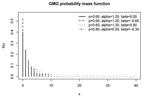
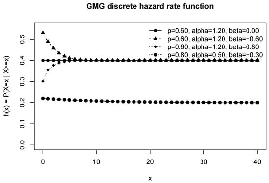
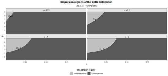
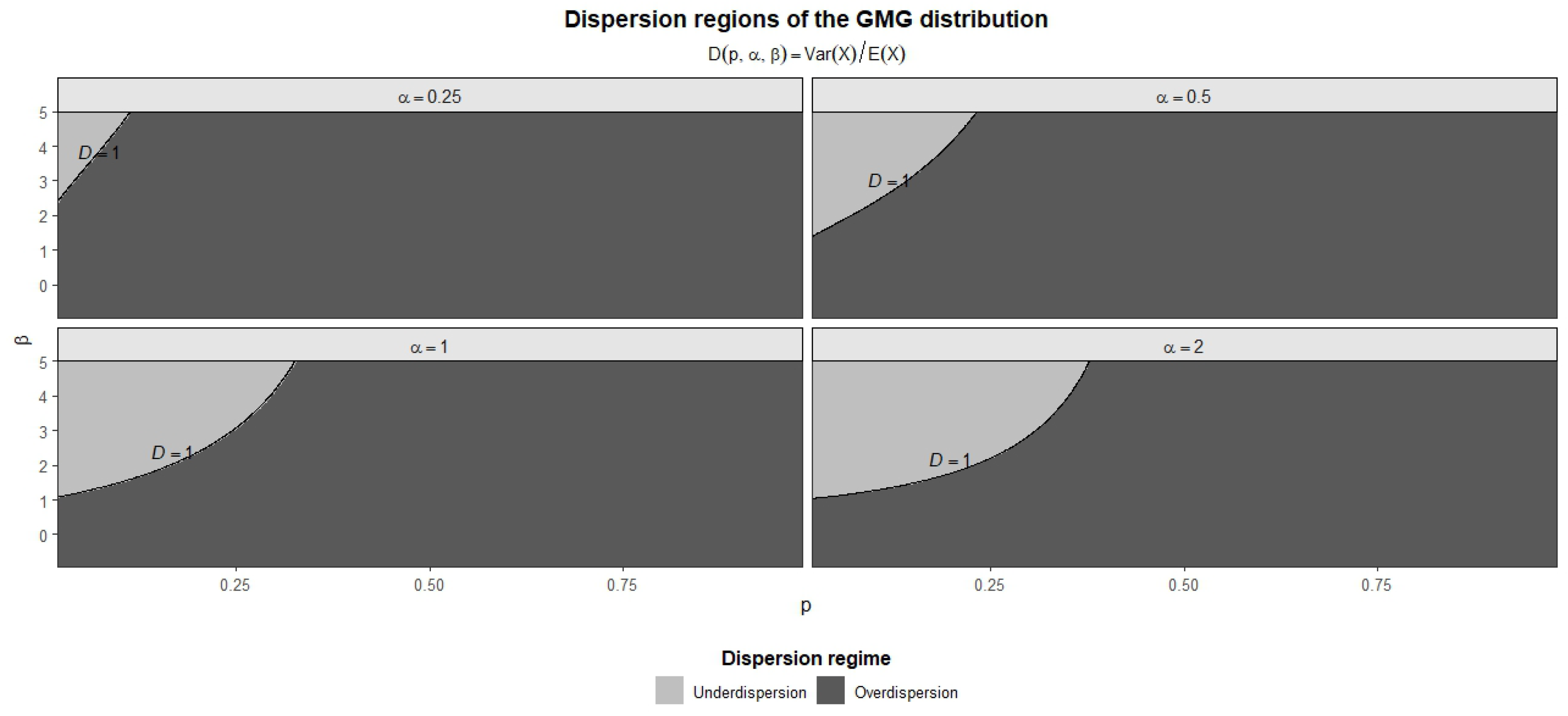
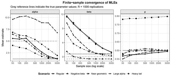
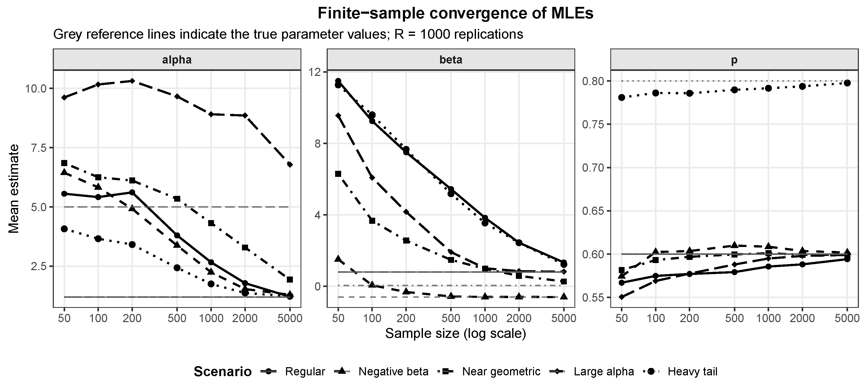
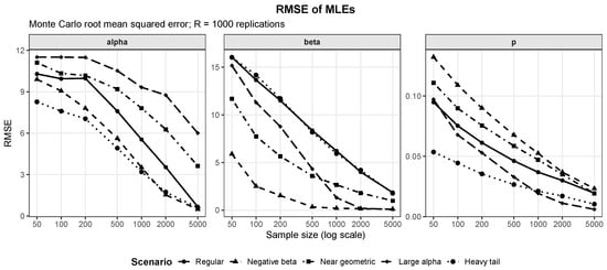
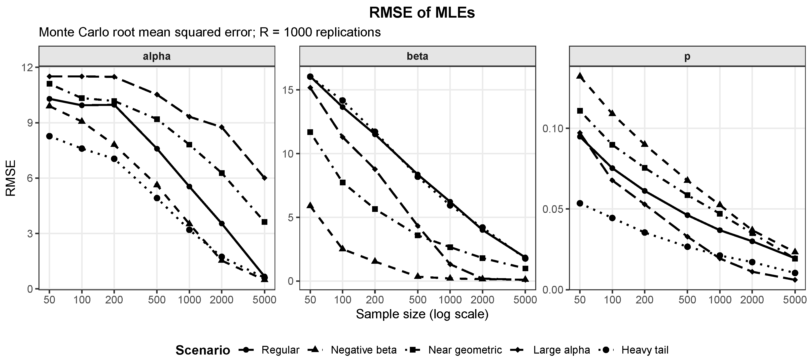
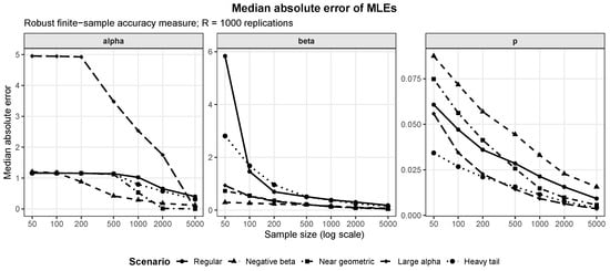
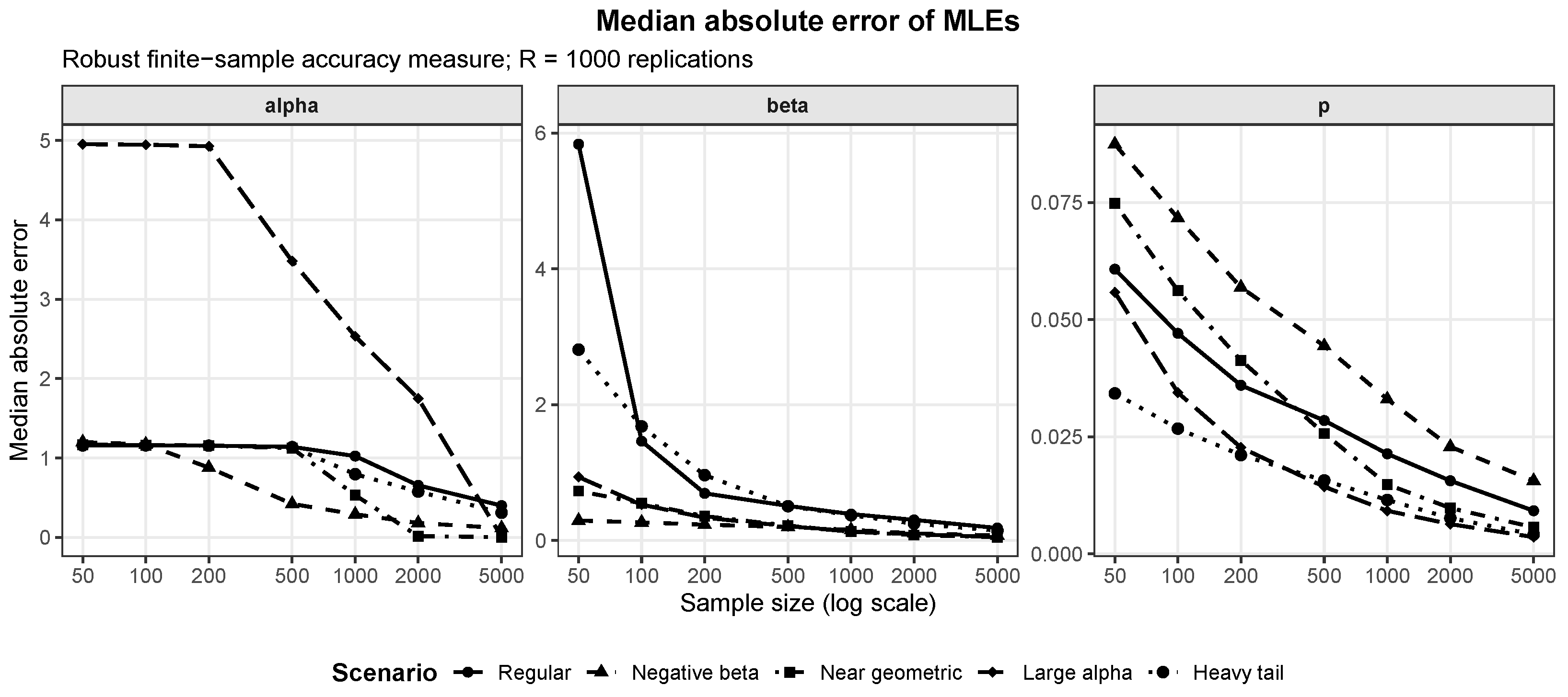
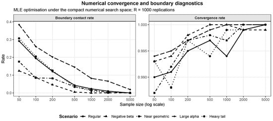
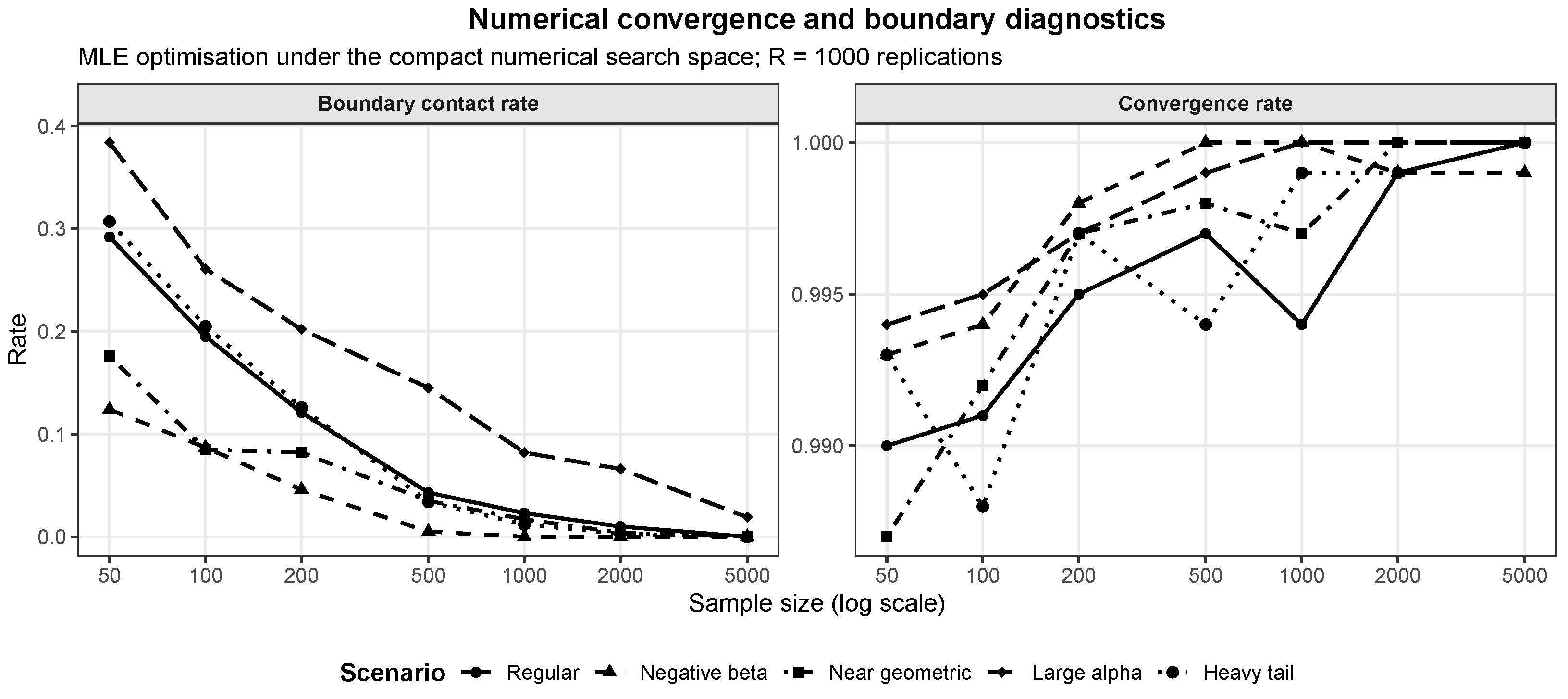

Disclaimer/Publisher’s Note: The statements, opinions and data contained in all publications are solely those of the individual author(s) and contributor(s) and not of MDPI and/or the editor(s). MDPI and/or the editor(s) disclaim responsibility for any injury to people or property resulting from any ideas, methods, instructions or products referred to in the content. |
© 2026 by the authors. Licensee MDPI, Basel, Switzerland. This article is an open access article distributed under the terms and conditions of the Creative Commons Attribution (CC BY) license.