Modelling South African Macroeconomic and Financial Time Series: A Comparative Analysis of Vector Autoregressive Moving Average and Asymmetric Generalised Autoregressive Conditional Heteroskedasticity Frameworks

Abstract

This study examines the modelling and forecasting of South African macroeconomic and financial time series using a comparative framework based on Vector Autoregressive (VAR), Vector Autoregressive Moving Average (VARMA), and GARCH-type models. Quarterly data spanning 1970 to 2024 were analysed to determine GDP growth, exchange rates, interest rates, and household consumption expenditure. VAR and VARMA models were employed to capture conditional mean dynamics, while GARCH, EGARCH, and GJR-GARCH models, including ARMA-GARCH extensions, were used to model volatility behaviour. Optimal model specifications were selected using the Akaike Information Criterion (AIC), Bayesian Information Criterion (BIC), Hannan–Quinn Criterion (HQ), and the Extended Cross-Correlation Matrix (ECCM), resulting in the estimation of VAR (4) and VARMA (1,1) models. The results reveal strong dynamic interdependencies among the variables. However, diagnostic tests indicate that the VAR (4) and VARMA (1,1) models do not fully capture the underlying data-generating process, as evidenced by residual autocorrelation, heteroskedasticity, and non-normality. Although the VARMA (1,1) model improved forecasting performance relative to the VAR (4) model, important nonlinear and higher-order dynamics remained unexplained. Volatility modelling revealed substantial persistence and clustering, particularly in exchange rates and interest rates. Initial GARCH, EGARCH, and GJR-GARCH specifications exhibited residual autocorrelation and remaining ARCH effects, suggesting model misspecification. The incorporation of an ARMA (1,1) term into the asymmetric GARCH models significantly improved model adequacy by eliminating residual autocorrelation and heteroskedasticity. Limited evidence of asymmetric volatility effects was found. Overall, the findings demonstrate that GARCH-ARMA specifications provide a more robust framework for modelling South Africa’s macroeconomic and financial dynamics. This study recommends future research incorporating nonlinear, regime-switching, and exogenous-variable models to enhance forecasting accuracy and policy relevance.

1. Introduction

Macroeconomic and financial time series modelling plays a central role in economic forecasting, policy formulation, risk management, and investment decision-making [1,2]. The increasing interconnectedness of economic and financial systems has intensified the need for robust multivariate modelling frameworks capable of capturing dynamic relationships, structural dependencies, and volatility transmission among key macroeconomic indicators [3]. In emerging economies such as South Africa, these challenges are particularly pronounced due to recurrent structural changes, policy uncertainty, exchange rate fluctuations, inflationary pressures, and external financial shocks [4,5]. Consequently, accurate modelling and forecasting of macroeconomic and financial variables remain critical for both policymakers and market participants.

Multivariate time series analysis provides a statistical framework for examining the interrelationships among economic variables over time. The rapid advancement of computational methods and statistical software has substantially expanded the application of multivariate econometric models in empirical research [3]. However, model selection remains a fundamental challenge, as inappropriate model specification and poor parameter estimation may produce biased forecasts and misleading inferences [6]. This has motivated continuous methodological developments aimed at improving forecasting accuracy and capturing the complex dynamics inherent in macroeconomic and financial systems.

Among the most widely applied linear multivariate frameworks are the Vector Autoregressive (VAR) and Vector Autoregressive Moving Average (VARMA) models. VAR models have become a standard tool in empirical macroeconomics because of their flexibility, simplicity, and ability to capture dynamic interdependencies among multiple endogenous variables without imposing restrictive theoretical assumptions [3,7]. Nevertheless, VAR models often require a large number of parameters and may fail to provide parsimonious representations of complex systems, particularly when higher-order lag structures are involved. In contrast, VARMA models extend the VAR framework by incorporating moving-average components, thereby offering a more compact and theoretically efficient representation of multivariate stochastic processes [1]. Despite their theoretical superiority, VARMA models remain underutilised in empirical applications because of identification difficulties, computational complexity, and estimation challenges, especially in developing-country contexts such as South Africa [3,8]. Additionally, ref. [9] conducted a review of VARMA models and indicated that these models are scarcely used in practice, as their adoption is complicated by identification, estimation, and specification difficulties. This has resulted in limited empirical advantages of VARMA models over VAR models. However, ref. [10] stated that, in small samples typical of macroeconomic data, VARMA models offer little advantage over VAR models in characterising the known data-generating processes (DGPs).

Beyond linear dependence structures, macroeconomic and financial time series frequently exhibit nonlinear characteristics such as volatility clustering, heteroskedasticity, leptokurtosis, and persistence in conditional variance. These stylised facts limit the adequacy of purely linear models for forecasting and risk assessment. To address these limitations, volatility-based models such as the Generalised Autoregressive Conditional Heteroskedasticity (GARCH) framework are commonly employed. Introduced as an extension of the ARCH model proposed by [11], GARCH models provide a parsimonious yet flexible structure for modelling time-varying volatility and capturing periods of financial turbulence and stability. Their application has become increasingly important in financial econometrics, particularly for understanding uncertainty, market risk, and the transmission of macroeconomic shocks.

Although extensive literature exists on VAR, VARMA, and GARCH modelling individually, relatively few studies provide an integrated comparative framework that jointly evaluates these approaches within the context of long-run South African macroeconomic and financial data. Existing studies often focus either on linear interdependencies or volatility modelling in isolation, thereby overlooking the potential complementarities between mean and variance dynamics. Furthermore, empirical evidence comparing the forecasting performance of VAR and VARMA models in emerging economies remains limited, despite the theoretical advantages associated with VARMA specifications.

This study addresses these gaps by developing a comprehensive comparative framework for modelling and forecasting South African macroeconomic and financial time series using VAR, VARMA, and GARCH models. Using quarterly data spanning 1970–2024, this study evaluates the ability of these models to capture dynamic interactions, structural behaviour, and volatility persistence across macroeconomic and financial indicators. Although VAR, VARMA and GARCH models address different aspects of time-series behaviour, they represent widely used forecasting approaches in macroeconomic analysis. VAR and VARMA focus on modelling multivariate mean dynamics, whereas GARCH captures time-varying volatility. This study evaluates their relative forecasting performance in order to identify the approach that provides the most accurate predictions for the variables under consideration.

This study contributes to the literature in several important ways. First, it provides one of the few empirical comparisons of VAR and VARMA models in the South African context, where applications of VARMA models remain relatively limited despite their theoretical advantages in capturing multivariate dynamics. Second, this study extends the analysis beyond linear mean models by incorporating symmetric and asymmetric volatility models, including GARCH, EGARCH, GJR-GARCH, and their ARMA-GARCH extensions, thereby offering a comprehensive assessment of both conditional mean and volatility dynamics. Third, it demonstrates that the inclusion of ARMA terms within asymmetric GARCH frameworks significantly improves model adequacy by eliminating residual autocorrelation and remaining ARCH effects, highlighting the importance of jointly modelling mean and variance processes. Fourth, this study employs rigorous model selection, diagnostic testing, and forecasting procedures using information criteria and forecast error measures to evaluate model performance. Finally, the findings provide practical insights for economic forecasting, risk assessment, and policy analysis in South Africa while identifying avenues for future research involving nonlinear, regime-switching, and exogenous-variable models.

By integrating these modelling approaches within a unified empirical framework, this study contributes both methodologically and empirically to the literature on multivariate macroeconomic and financial forecasting in emerging economies. The findings are expected to provide valuable insights for policymakers, researchers, financial analysts, and investors seeking to better understand the dynamics and predictability of South African macroeconomic and financial systems.

The remainder of the paper is organised as follows. Section 2 reviews the relevant literature on multivariate time series and volatility modelling. Section 3 presents the data and methodology employed in the study. Section 4 discusses the empirical findings and forecasting results. Finally, Section 5 concludes the paper and provides recommendations for future research.

2. Literature Review

2.1. VAR and VECM Models in Macroeconomic Forecasting

Multivariate time series models, particularly VAR, VARMA, and GARCH-type models, have been extensively applied in both developed and emerging economies to analyse and forecast macroeconomic and financial variables. Ref. [12] applied VAR and VECM methodologies to model inflation dynamics in Ethiopia using annual data (1992–2021). The study identified at least one long-run cointegrating relationship among inflation, GDP, government expenditure, money supply, and imports. The VECM results confirmed convergence towards long-run equilibrium, while VAR-based forecasts revealed fluctuating inflation trends in the short term.

In the South African context, ref. [13] examined the effects of oil price shocks and exchange rate movements (ZAR/USD) on consumer prices using VAR and Structural VAR (SVAR) models. Their findings revealed that oil price shocks lead to short-term increases in consumer prices and an initial appreciation of the rand. However, long-run SVAR results indicated sustained rand depreciation and lower consumer prices, suggesting a deflationary effect. These results highlight the vulnerability of South Africa as a net oil importer and the importance of distinguishing between short- and long-run dynamics.

2.2. VARMA and Advanced Multivariate Forecasting Model

Ref. [14] demonstrated the advantages of VARMA models in impulse-response analysis and forecasting, proposing improved estimation techniques and information criteria. Similarly, ref. [15] compared VARMA with steady-state Bayesian VAR (BVAR) and benchmark AR models for Swedish macroeconomic data (1993–2024). Their findings showed that while VARMA can outperform classical VAR models, the steady-state BVAR provided superior forecasting accuracy, highlighting the importance of model selection in macroeconomic forecasting.

Recent advancements have focused on addressing limitations of traditional VAR and VARMA models. Ref. [16] introduced a Time-Varying Scalar Component VARMA (TV-SCVARMA) model to account for structural instability and parameter nonlinearity in macroeconomic data. Using quarterly Nigerian data (2010Q1–2024Q1), the study demonstrated that the proposed model outperformed classical VARMA in forecasting accuracy, as measured by RMSE, and produced more stable forecasts. The authors recommend time-varying parameter models for economies characterised by structural instability.

2.3. GARCH Models and Volatility Dynamics

In terms of volatility modelling, GARCH-type models remain fundamental in capturing nonlinearities and volatility clustering in financial and macroeconomic time series. Ref. [17] applied ARCH, GARCH, and EGARCH models to South African oil prices, showing that macroeconomic variables significantly influence volatility, with asymmetric effects evident under EGARCH. Similarly, ref. [18] compared several GARCH-type models across crude oil markets and found that APARCH outperformed alternative specifications in capturing volatility persistence and distributional characteristics. Additionally, ref. [19] found that the GARCH-type framework, particularly the GARCH-Mixed Data Sampling (GARCH-MIDAS) model, effectively extracts time-varying volatility and captures periods of heightened economic uncertainty through volatility clustering and macroeconomic uncertainty effects. Furthermore, ref. [20] found that GARCH-type models (standard GARCH and EGARCH) effectively modelled the persistent volatility clustering and macroeconomic shocks in GDP growth series.

The application of these models has also been extended to crisis contexts. Ref. [21] analysed the impact of COVID-19 on Casablanca’s stock market using GARCH(1,1), VAR-X, and Markov-Switching models. Their findings indicated that pandemic-related cases and deaths significantly influenced market volatility, with evidence of a structural break in stock returns during early 2020. Collectively, these studies highlight several key insights: VAR models are widely used due to their simplicity, while VARMA models offer a more parsimonious representation but are computationally demanding; forecasting performance varies across models and contexts, with emerging evidence supporting more advanced frameworks such as Bayesian and time-varying models; GARCH-type models are effective in capturing volatility clustering and asymmetry; and macroeconomic dynamics often exhibit both linear interdependencies and nonlinear volatility patterns.

Ref. [22] employed a structural break GARCH-MIDAS model, which combines high-frequency financial data with low-frequency macroeconomic variables while explicitly accounting for structural changes in market behaviour. Their findings revealed that monetary policy contains valuable information for explaining and forecasting cryptocurrency volatility, particularly during periods of economic uncertainty and financial instability. By incorporating structural breaks, the model was able to capture shifts in volatility regimes more effectively than conventional volatility models. Similarly, [23] utilised structural break econometric techniques and time series analysis to examine the impact of the United States financial crisis on macroeconomic variables within BRICS economies. Their approach focused on identifying regime shifts and testing the stability of macroeconomic relationships in the presence of major global shocks. The results demonstrated that the financial crisis introduced significant structural changes in macroeconomic series, highlighting the limitations of traditional models that assume parameter stability over time.

Despite extensive applications of VAR, VARMA, and GARCH-type models, limited evidence exists on their comparative forecasting performance using long-span South African macroeconomic data. In particular, few studies have evaluated whether the parsimonious representation of VARMA models offers forecasting advantages over conventional VAR models while simultaneously characterising the volatility dynamics of the variables under consideration. Addressing this gap may provide insights into the suitability of alternative modelling approaches for short-run macroeconomic forecasting in South Africa.

3. Methodology

This section discusses the dataset, preliminary analysis, and methodological framework employed in this study.

3.1. Data Preparation

3.1.1. Data

This study analyses South Africa’s macroeconomic and financial time series data from 1970:Q1 to 2024:Q4, consisting of 220 observations sourced from the South African Reserve Bank and Statistics South Africa. It includes endogenous variables such as the GDP growth rate, exchange rate (USD), interest rates and final consumption expenditure by households. The choice of the data period was dependent on the availability of the data from the sources at the time the analysis was computed. The data is publicly available from the two sources. The analysis was performed using Python (Colab) and R-studio: 2022.07.1554.

3.1.2. Preliminary Data Analysis

Time series variables are naturally non-stationary, requiring the first action of plotting the series to uncover patterns and trends over time. The formal Augmented Dickey–Fuller (ADF), Phillips-Perron (PP) and Kwiatkowski–Phillips–Schmidt–Shin (KPSS) tests for unit root are used to assess the stationarity of variables and identify their order of integration. The computed ADF and PP statistics are given by the following equations, respectively:

$$ADFstatistic=t_{\gamma }={\displaystyle \frac{\widehat{\gamma }}{SE\left(\widehat{\gamma }\right)}},$$

(1)

$$PP statistic=z_t=\sqrt{{\displaystyle \frac{{\widehat{\gamma }}_{0,n}}{{\widehat{\mathsf{\lambda }}}_n^2}}}{t}_{\widehat{\rho }}-{\displaystyle \frac{T({\widehat{\mathsf{\lambda }}}_n^2-{\widehat{\gamma }}_{0,n})}{2{\widehat{\mathsf{\lambda }}}_{n^s}}},$$

(2)

where $\widehat{\gamma }$ is the OLS estimate of $\gamma$, and $SE\left(\widehat{\gamma }\right)$ is its standard error. With respect to the PP statistic, T is the sample size, ${\widehat{\gamma }}_{0,n}$ is the short-run variance and ${\widehat{\mathsf{\lambda }}}_n^2$ is the long-run constant variance estimate. The KPSS test statistic is based on the cumulative sum of the residuals from the regression $x_t=\alpha +{\beta }_t+u_t+e_t$ on a constant and trend. It is computed using

$$KPSS statistic={\displaystyle \frac{T^{-2}{\displaystyle {\sum }_{t=1}^T}{S}_t^2}{{\widehat{\mathsf{\lambda }}}_T^2}},$$

(3)

where $S_t={\displaystyle {\sum }_{i=1}^t}{\widehat{e}}_i$ is partial sum of process of OLS residuals (${\widehat{e}}_i$) from the regression ($x_t$), and ${\widehat{\mathsf{\lambda }}}_T^2$ is a consistent estimate of long-run variance of the error term $e_t$.

3.2. Vector Autoregressive (VAR) Model

The VAR model, specifically $VAR\left(p\right)$, serves as a significant advancement over traditional large-scale macro-econometric models, which are typically estimated using Ordinary Least Squares (OLS) and Generalised Methods of Moments (GMM). VAR models extend univariate autoregressive models to multivariate time series, efficiently capturing the dynamic behavior of various macroeconomic and financial variables [24]. Choosing the correct lag order, denoted as $p$ in VAR(P) models, is critical for accurate model performance; an improper selection can induce substantial distortions. Various methods exist for determining the optimal $p$. This study utilises the information criteria approach for $VAR\left(p\right)$ model selection, as highlighted by [2]). This study focuses on three commonly employed information criteria: Akaike Information Criterion (AIC), Bayesian Information Criterion (BIC), and Hannan–Quinn Information Criterion (HQIC), calculated as follows:

$$AIC(p)=\mathit{ln}\left|{\widehat{\sum }}_{a,p}\right|+{\displaystyle \frac{2}{T}}{pk}^2,$$

(4)

$$\mathit{BIC}(p)=\mathit{ln}\left|{\widehat{\sum }}_{a,p}\right|+{\displaystyle \frac{ln(T)}{T}}{pk}^2,$$

(5)

$$HQ(p)=\mathit{ln}\left|{\widehat{\sum }}_{a,p}\right|+{\displaystyle \frac{2ln\left[\mathit{ln}\left(T\right)\right]}{T}}{pk}^2,$$

(6)

where $T$ is the sample size, and ${{\displaystyle \widehat{\sum }}}_{a,p}$ is the maximum likelihood (ML) estimate of ${\sum }_a$. The lag order $p$ that yields the lowest value from these criteria will be selected for further analysis within the VAR model. The $VAR\left(p\right)$ model can be estimated by various methodologies, including Least Squares (LS), Maximum Likelihood (ML), or Bayesian methods. Ref. [2] noted that LS estimation is asymptotically equivalent to ML estimates, while OLS is akin to Generalised Least Squares (GLS) estimates. The general structure of the $VAR\left(p\right)$ model is expressed as

$$Y=\varrho x+U=C_t+{\displaystyle {\sum }_{i=1}^p}{\Phi }_i{y}_{t-i}+u_t,$$

(7)

where $\mathrm{Y}$ is an $(n\times 1)$ vector of stationary time series, ${\mathrm{C}}_t$ is the constant vector, $\mathsf{\varrho }$ is a vector of parameters, also represented as ${\Phi }_i$, and $u_t$ is the unobservable zero mean white noise vector process (serially uncorrelated or independent). LS estimation is preferred for its simplicity and efficiency, ensuring unbiased estimations under the condition that all regressors are predefined, and the error components exhibit white noise characteristics.

Finally, the diagnostic checking of the $VAR\left(p\right)$ model requires assessment of residuals to ensure independence across periods. Any significant correlation in residuals indicates serial correlation and suggests inadequacies in model fitting, thus necessitating revisiting the model dynamics for improvements. This thorough approach underscores the critical importance of lag selection, parameter estimation, and diagnostic testing in VAR modelling for time series analysis.

3.3. Vector Autoregressive Moving Average (VARMA) Model

A VARMA model is a statistical time series process for analysing and forecasting multiple interdependent time series by capturing their complex dynamic relationships [25]. The $VARMA(p,q)$ model is an extension of the popular $VAR\left(p\right)$ model by adding MA terms accounting for past forecast errors to provide more precise, parsimonious predictions and handling unexpected shocks better than simpler $VAR\left(p\right)$ models. As for $VAR\left(p\right)$ models, it is of prime importance to correctly specify the order of p and q for the $VARMA(p,q)$ model. The extended cross correlation matrices (ECCM) are powerful identification tool for determining the order $(p,q)$ of VARMA model [2]. ECCM helps identify the AR and MA orders $(p,q)$ that produce parsimonious, well-fitting models; hence, it is used in this study to identify the order $(p,q)$ of VARMA models. Since $p$ and $q$ are not known, the two-way table of probability values of the multivariate Ljung–Box statistics $Q_{\left(j+1\right):l}^{\upsilon }$ for $j=0,1,\dots \dots ,l$ and $\upsilon =0,1,\dots \dots ,m$ is considered, where $l$ is the maximum pre-specified MA order $\left(q\right),$ and $m$ is the maximum pre-specified AR order $\left(p\right)$. The Ljung–Box statistic is presented as

$$Q_{\left(j+1\right):l}^{\upsilon }=T^2{\displaystyle {\sum }_{\upsilon =j+1}^l}{\displaystyle \frac{1}{T-\upsilon }}tr[{\Gamma }_{\upsilon }^{\prime }(w_{mt}^{\left(j\right)}){\Gamma }_0^{-1}(w_{mt}^{\left(j\right)}){\Gamma }_{\upsilon }(w_{mt}^{\left(j\right)}){\Gamma }_0^{-1}(w_{mt}^{\left(j\right)})],$$

(8)

Based on the null hypothesis that $z_t$ follows the $VARMA(m,j)$ model, $Q_{\left(j+1\right):l}^n$ is asymptotically a chi-square (${\chi }^2$) with the degrees of freedom $K^2\left(l-j\right)-\mathrm{r}$. The p-value associated with $Q_{\left(j+1\right):l}^n$ is denoted as $p_{mj}$. The DGP of the $K$ dimensional multiple time series, $y_t,\dots \dots y_K$, is stationary—that is, the first and the second moments are time invariant [1]. The VARMA process has finite order and can be represented in the general form as

$${A_0{y}_t=A}_1{y}_{t-1}+\cdots +A_p{y}_{t-p}+M_0{u}_t+M_1{u}_{t-1}+\cdots +M_q{u}_{t-q},$$

(9)

where Ai denotes the AR parameters, and Mi represents the MA parameters. This VARMA(p,q) model can also be presented as follows:

$${\mathsf{\Phi }}_0{y}_t={\mathsf{\Phi }}_1{y}_{t-1}+\cdots {\mathsf{\Phi }}_p{y}_{t-p}+{\mathrm{ɵ}}_0{u}_t+{\mathrm{ɵ}}_1{u}_{t-1}+\cdots {\mathrm{ɵ}}_q{u}_{t-q},$$

(10)

where $\mathsf{\Phi }$ and ɵ (equal to A and M in Equation (9), respectively) represent the AR and MA parameters. The $VARMA(p,q)$ model in either Equation (9) or (10) in this instance is assumed to be stationary and uniquely defined as in the echelon form and can be rearranged as

$$Y=\varrho x+U,$$

(11)

where $Y=(y_1,\dots ,y_T)$ is of dimension $(K\times T)$, U = ($u_1,\dots {,u}_T$) is of dimension $(K\times T)$, $\varrho =\left[\right(IK-{\Phi }_0),{\Phi }_1,\dots \dots ,{\Phi }_p$, $({\mathrm{ɵ}}_0-IK)$, ${\mathrm{ɵ}}_1$,….., ${\mathrm{ɵ}}_q$] is the $(K\times K(p+q+2\left)\right)$ vector of parameters, $X_t=[y_t{,y}_{t-1},\dots \dots ,u_1,u_{t-1},\dots \dots ,u_{t-q}]$, and $X=[X_0,\dots \dots ,X_T]$ is the $\left(k\right(p+q+2)\times T)$ and is the matrix of regressors. If the Vec operator is applied to Equation (11), then

$$Vec\left(Y\right)=\left(X^{\prime }\otimes I_K\right)Vec\left({\varrho }^{\prime }\right)+Vec\left(U\right),$$

(12)

Suppose there is an echelon form transformation, i.e., a transformation in which some of the elements in the vector of parameters, where $\varrho$ are equated towards zero (0), implying that ${\mathsf{\Phi }}_0$ = ${\mathrm{ɵ}}_1$ and $\varrho$ will now be of dimension $(K\times K(p+q+1\left)\right)$ and $\otimes$ denotes the tensor product. In that, $\varrho$ can be allowed to be written as a linear combination of a matrix and a vector of Rλ, where R is a matrix consisting of 0s and 1s that is applied by transformation and is of dimension $(K^2\left(p+q+1\right)\times K^2(p+q+1\left)\right)$. ${\mathsf{\varrho }}^{*}=\mathrm{V}\mathrm{e}\mathrm{c}({\mathsf{\Phi }}_0,{\mathsf{\Phi }}_1,\dots \dots ,{\mathsf{\Phi }}_p,{\mathrm{ɵ}}_1,\dots ..,{\mathrm{ɵ}}_q)$ is a ($K^2(p+q+1)\times 1)$ matrix that contains all of the $K^2(p+q+1)$ parameters that are required to be estimated. Following this, Equation (11) can be estimated as follows:

$$Vec\left(Y\right)=\left(X^{\prime }\otimes I_K\right)R{\varrho }^{*}+Vec\left(U\right).$$

(13)

There are still limitations, as X contains values of the error terms that are not fully observed. A consistent estimator $\widehat{{\mathrm{U}}_{\mathsf{ı}}}$, therefore, needs to be computed, and it is performed by expressing the $VARMA(p,q)$ model in a VAR representation, as the model is assumed to be invertible. Thus, $\widehat{{\mathrm{U}}_0}$ is computed as follows:

$$\widehat{{\mathrm{U}}_{0,t}}=y_t-{\sum }_{i=1}^p{\prod }_i{y}_{t-\mathrm{i}}.$$

(14)

From Equation (14), the new matrix of regressors is obtained by substituting $\widehat{{\mathrm{U}}_{0,t}}$ into the original matrix $X_t$; consequently, the matrix of regressors is $X_0$. The initial estimator for ${\mathsf{\varrho }}^{*}$, ${\widehat{\mathsf{\varrho }}}_1^{*}$ is expressed as

$${\widehat{\mathsf{\varrho }}}_1^{*}={\left[R^{\prime }\right(X_0,X_0^{\prime })\otimes I_K)\mathrm{R}]}^{-1}\mathrm{R}(X_0^{\prime }\otimes I_k)\mathrm{V}\mathrm{e}\mathrm{c}(\mathrm{Y}).$$

(15)

The parameter matrices, ${\widehat{\mathsf{\Phi }}}_{0,t},\dots \dots ,{\widehat{\mathsf{\Phi }}}_{1,p},{\widehat{\mathrm{ɵ}}}_{\mathrm{1,0}},\dots \dots ,{\widehat{\mathrm{ɵ}}}_{1,q}$, can be computed recursively from a new set of residuals ${\widehat{\mathrm{U}}}_{1,t}$ where the first subscript represents the iteration number, and the second subscript represents the lag order. Therefore, ${\widehat{\mathrm{U}}}_{1,t}$ is estimated as

$${\widehat{\mathrm{U}}}_{1,t}=y_t-{\widehat{\mathsf{\Phi }}}_{\mathrm{1,0}}^{-1}{{\displaystyle {\sum }_{i=1}^p}\widehat{\mathsf{\Phi }}}_{1,\mathrm{i}}{y}_{t-1}-{\widehat{\mathsf{\Phi }}}_{\mathrm{1,0}}^{-1}{{\displaystyle {\sum }_{i=1}^q}\widehat{\mathrm{ɵ}}}_{1,i}{\widehat{\mathrm{U}}}_{1,i}{y}_{t-1}.$$

(16)

In general, the LSE at the jth iteration ${\widehat{\mathsf{\varrho }}}_j^{*}$ is expressed as

$${\widehat{\mathsf{\varrho }}}_j^{*}={[R^{\prime }\left(X_{j-1}{X}_{j-1}^{\prime }\right)\otimes I_K)R]}^{-1}R\prime \left(X_{j-1}^{\prime }\otimes I_K\right)Vec(Y),$$

(17)

and

$${\widehat{\mathrm{U}}}_{j,t}=y_t-{\widehat{\mathsf{\Phi }}}_{j,0}^{-1}{\displaystyle {\sum }_{i=1}^p}{\widehat{\mathsf{\Phi }}}_{j,\mathrm{i}}{y}_{t-\mathrm{i}}-{\widehat{\mathsf{\Phi }}}_{j,0}^{-1}{\displaystyle {\sum }_{i=1}^q}{\widehat{\mathrm{ɵ}}}_{j,\mathrm{i}}{\widehat{\mathrm{U}}}_{j,t-\mathrm{i}}.$$

(18)

The jth iteration in which the vector of parameter estimated converges, i.e., || ${\widehat{\mathrm{U}}}_{t,j+1}-{\widehat{\mathrm{U}}}_{t,j}$|| < (pre-specified constant) terminates the procedure. The LSE at this point is taken as ${\widehat{\mathsf{\varrho }}}_j^{*}$. Ref. [26] noted that this estimator is feasible for higher-dimensional models in contrast to those of MLE.

3.4. Generalised Autoregressive Conditional Heteroskedasticity Model

The univariate ARCH model was introduced by [11], with the GARCH model proposed by [27] as its extension. Various extensions exist, including the EGRACH and IGRACH models, which are not covered in this study. Instead, this study utilises the GARCH model to analyse the volatility of macroeconomic and financial time series in South Africa, applying a similar equation as $ARCH(1,1)$ for long-returns $r_t$, incorporating additional terms for volatility, and that is

$$\begin{array}{l}{r}_t={\sigma }_t{\epsilon }_t,{\epsilon }_t~N(0,1)\\ {\sigma }_t^2={\alpha }_0+{\displaystyle {\sum }_{i=1}^q}{\alpha }_{\mathrm{i}}{r}_{t-\mathrm{i}}^2,\end{array}$$

(19)

where $t>max(p,q)$, and the remaining components are as in the ARCH model. The parameters of the model are ${\alpha }_0{,\alpha }_1,\dots {\alpha }_q,$ where $q$ is a positive integer. Equation (19) therefore represents the $ARCH\left(q\right)$ specification, obtained as a special case of the GARCH model when $p=0$. Hence, the GARCH model generalises the ARCH by introducing values of ${\sigma }_{t-1}^2,{\sigma }_{t-2}^2,\dots ,{\sigma }_{t-i}^2$ in the equation. Let {$r_t$} be the mean corrected return, and ${\epsilon }_t$ denote a Gaussian white noise with zero mean and unit variance. Let also $H_t$ be the information set at time t given by $H_t=\{r_1,r_2,\dots ,r_{t-1}\}$; then, the process of GARCH (1,1) is

$$r_t={\sigma }_t{\epsilon }_t,{\epsilon }_t~N(0,1),$$

(20)

and

$${\sigma }_t^2={\alpha }_0+{\displaystyle {\sum }_{i=1}^q}{\alpha }_{\mathrm{i}}{r}_{t-\mathrm{i}}^2+{\displaystyle {\sum }_{j=1}^p}{\beta }_{\mathrm{j}}{\sigma }_{t-\mathrm{j}}^2$$

(21)

where ${\alpha }_0>0$, ${\alpha }_{\mathrm{i}}\ge 0$ and ${\beta }_{\mathrm{j}}\ge 0$. When comparing among different specifications of GARCH models, the appropriate model is selected based on AIC, SBC and HQC. A model with the minimum value of AIC, SBC, and HQC will be selected. Forecasting with the $GARCH(p,q)$ model parallels the ARMA model. The conditional variance of $\left\{r_t\right\}$ derives from the conditional expectation of mean-corrected returns, with one-step ahead volatility forecasted from a given origin $T$ presented as follows:

$$\begin{array}{l}{\widehat{r}}_{t+1}^2=E[r_{t+1}^2\mathrm{|}{r}_t]\\ ={\alpha }_0+{\displaystyle {\sum }_{i=1}^q}{\alpha }_i{r}_{t+1-i}^2\mp {\displaystyle {\sum }_{j=1}^p}{\beta }_j{\sigma }_{t+1-j}^2,\end{array}$$

(22)

where $E[r_{t+1}^2\mathrm{|}{r}_t]$ for $i<\mathsf{ı}$ can be given recursively as for $i\ge \mathsf{ı},E({\sigma }_{t+1-j}^2\mathrm{|}{r}_t)=0$ $for i<\mathsf{ı},E({\sigma }_{t+1-j}^2\mathrm{|}{r}_t)=v_{t+\mathsf{ı}-i}$ for $i\ge \mathsf{ı}$.

3.5. Asymmetric GARCH Models

Financial markets often exhibit asymmetric responses, where negative news tends to have a greater impact on volatility than positive news of the same magnitude. To address this limitation, the EGARCH model was developed. The EGARCH model allows positive and negative shocks to have different effects on volatility and accommodates the possibility that larger shocks exert a greater influence on volatility than is assumed under the standard GARCH framework [28]. According to ref. [28], the conditional variance of Nelson’s EGARCH $(p,q)$ model is written as

$$\ln \left({\sigma }_t^2\right)=\omega +{\beta }_1\ln \left({\sigma }_{t-1}^2\right)+{\alpha }_1\left\{\left|{\displaystyle \frac{{\epsilon }_{t-1}}{{\sigma }_{t-1}}}\right|-\sqrt{{\displaystyle \frac{2}{\pi }}}\right\}-\gamma {\displaystyle \frac{{\epsilon }_{t-1}}{{\sigma }_{t-1}}}$$

(23)

where $\omega$ is the constant term, ${\beta }_1\ln \left({\sigma }_{t-1}^2\right)$ denotes the fitted variance from the previous period, and $\gamma$ is the value of the leverage term if the value of $\gamma >0$, where it is concluded that there is a larger impact for negative shocks on the conditional variance. The GJR-GARCH $(p,q)$ model is the other asymmetric GARCH model used in the study. According to ref. [29], the general form of this model is expressed as follows:

$${\zeta }_t^2=\omega +{\Sigma }_{i=1}^p{\alpha }_i{\epsilon }_t^2+{\Sigma }_{j=1}^q{\beta }_j{\sigma }_{t-j}^2+{\Sigma }_{i=1}^p{\gamma }_i{I}_{t-i}{\epsilon }_{t-1}^2$$

(24)

where; $I_{t-i}=1$ if ${\epsilon }_{t-i}<0$, or $0 \mathrm{i}\mathrm{f} {\epsilon }_{t-i}\ge 0$. The variance equation is written as

$${\zeta }_t^2=\omega +{\alpha }_1{\epsilon }_t^2+{\beta }_1{\sigma }_{t-1}^2+{\gamma }_i{I}_{t-1}{\epsilon }_{t-1}^2.$$

(25)

3.6. Hybrid Model

To simultaneously model the conditional mean and volatility dynamics of the macroeconomic and financial series, this study employed $EGARCH(1,1)$ and $GJR-GARCH(1,1)$ with $ARMA(1,1)$ specifications. The $ARMA\left(1,1\right)$ component captures linear dependence in the mean equation, while the EGARCH and GJR-GARCH components model time-varying volatility, volatility clustering, persistence, and potential asymmetric responses of volatility to shocks. The conditional mean equation for both models is given as

$$y_t=\mu +\phi y_{t-1}+\theta {\epsilon }_{t-1}+{\epsilon }_t$$

(26)

where $y_t$ is the observed series, $\mu$ is a constant, $\phi$ is the autoregressive coefficient, $\theta$ is the moving-average coefficient, and ${\epsilon }_t$ is the error term. The error term is assumed to follow ${\epsilon }_t=z_t\sqrt{h_t},$ where $z_t$ is an independently and identically distributed process with zero mean and unit variance, and $h_t$ is the conditional variance. The EGARCH and GJR-GARCH variance equations are computed using

$$\ln \left(h_t\right)=\omega +\alpha \left({\displaystyle \frac{\left|{\epsilon }_{t-1}\right|}{\sqrt{h_{t-1}}}}-E\left[{\displaystyle \frac{\left|{\epsilon }_{t-1}\right|}{\sqrt{h_{t-1}}}}\right]\right)+\gamma {\displaystyle \frac{{\epsilon }_{t-1}}{\sqrt{h_{t-1}}}}+\beta (h_{t-1})$$

(27)

$$h_t=\omega +\alpha {\epsilon }_{t-1}^2+\gamma I_{t-1}{\epsilon }_{t-1}^2+\beta h_{t-1}$$

(28)

where $\omega$ is the constant variance parameter, $\alpha$ measures the magnitude effect of shocks, $\beta$ captures volatility persistence, $I_{t-1}$ is an indicator function equal to 1 when ${\epsilon }_{t-1}<0$ and 0 otherwise and γ represents the asymmetry or leverage effect. A statistically significant $\gamma$ indicates that positive and negative shocks have different effects on future volatility. The logarithmic specification ensures that the conditional variance remains positive without imposing non-negativity restrictions on the parameters.

4. Discussion of Results

This section of the study presents the results of the data analysis and discussions of the results obtained from the findings. The findings are presented using tables and figures.

Preliminary Data Analysis

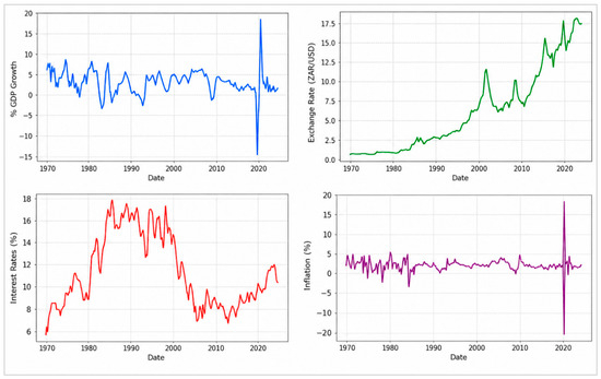
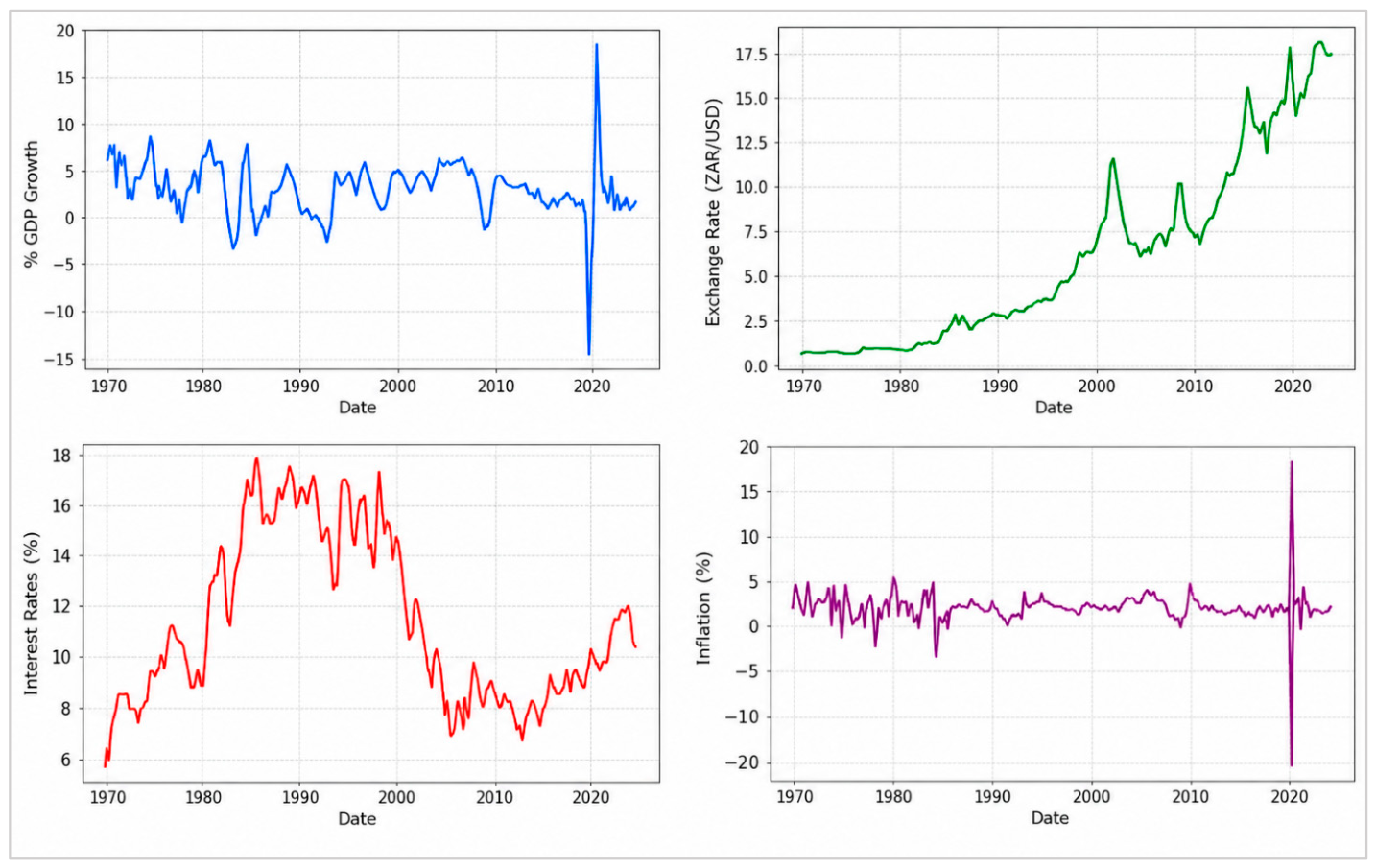
The starting point of time series analysis is the visual inspection of time series plots of macroeconomic and financial time series variables. The line plots of time series values against time highlight the possible patterns and trends that are naturally in the data over time. Figure 1 presents the time series variables under study.

Figure 1. Time series plots.

South Africa’s GDP growth (1970–2024) averaged about 2.6%, with periods of strong growth in the 1970s and 1980s followed by declines due to factors such as oil price shocks, sanctions during Apartheid, and global crises. Major events, including the 2007–2009 financial crisis and COVID-19, caused sharp contractions and rebounds. The GDP series exhibits fluctuations and non-stationarity. The exchange rate shows a long-term upward (depreciating) trend with notable fluctuations, also indicating non-stationarity. Interest rates rose until the late 1980s, then declined post-1999 due to improved macroeconomic management, but remain non-stationary. In contrast, household consumption is relatively stable and stationary, with a temporary drop during COVID-19. Unit root tests are applied to confirm these properties.

Table 1 presents a summary of the results for ADF, PP and KPSS stationary tests. The results revealed that GDP growth rate and final consumption expenditure by households (FCEHH) are stationary at levels, while the exchange rate (USD) and South Africa’s interest rate are non-stationary at levels. However, all variables are integrated of order 1 (I (1)) to stabilise their mean and variance to obtain stationarity for modelling the time series under study to ensure that the VAR/VARMA modelling approaches are estimated using a common order of integration. This decision was made to satisfy the stationarity assumptions underlying multivariate time-series models, improve the comparability of parameter estimates across variables, and minimise the risk of spurious inference that may result from combining stationary and non-stationary series within the same system. According to ref. [30], ensuring stationarity is fundamental for valid estimation and inference in VAR systems, particularly when the objective is forecasting. Similarly, ref. [31] emphasises that differencing variables to achieve a stationary system is an appropriate strategy when modelling short-run dynamics and when cointegration is not the primary focus.

Table 1. The results of ADF, PP and KPSS unit root tests.

Variable (S)	Level of Test	ADF		PP		KPSS		Conclusion
		t-Statistic	p-Value	t-Statistic	p-Value	t-Statistic	p-Value
GDP growth rate	Level	−5.819	0.000	−5.414	0.000	0.288	0.100	Stationary
	1st Difference	−13.136	0.000	−20.617	0.000	0.014	0.100	Stationary
Exchange Rates (USD)	Level	−2.292	0.436	−2.009	0.596	0.653	0.001	Non-Stationary
	1st Difference	−10.555	0.000	−11.621	0.000	0.023	0.100	Stationary
Interest Rates	Level	−2.399	0.379	−2.252	0.461	0.729	0.001	Non-Stationary
	1st Difference	−10.461	0.000	−12.469	0.000	0.233	0.100	Stationary
FCEHH	Level	−10.233	0.000	−16.707	0.000	3.015	0.100	Stationary
	1st Difference	−21.162	0.000	−32.708	0.000	0.296	0.100	Stationary

Table 2 shows the selection of VAR lag order based on different information criteria. AIC and HQIC suggest that a $VAR\left(4\right)$ model is the best choice, yielding values of −0.373 and 0.067. Conversely, BIC supports the $VAR(3$) model, resulting in the minimal value of 0.627. AIC and BIC focus on reducing the anticipated Kullback–Leibler distance to the actual model, while BIC reliably chooses the simplest model. HQIC, recognised for its selection of autocorrelation models, endorses the selection of $VAR\left(4\right)$ for further analysis.

Table 2. VAR model selection.

P	AIC (n)	HQ (n)	SC (n)	FPE (n)	p-Value
1	1.18564	1.31496	1.50548	3.27291	<0.000
2	0.99966	1.23242	1.57537	2.71793	<0.000
3	−0.2044	0.13184	0.62721	0.81568	<0.000
4	−0.3728	0.06688	0.71467	0.68981	<0.000
5	−0.3211	0.22204	1.02225	0.72735	<0.000
6	−0.2146	0.43199	1.38463	0.81061	0.300
7	−0.3438	0.40626	1.51132	0.71423	0.931
8	−0.3582	0.49531	1.75279	0.70645	<0.000
9	−0.282	0.67488	2.08478	0.7657	0.021
10	−0.2482	0.81216	2.37448	0.79644	0.658
Selected Oder: AIC = 4, BIC = 3, HQ = 4

Table 3 presents the p-values from the Extended Cross-Correlation Matrix (ECCM) used for preliminary VARMA order identification. The ECCM procedure was applied using a 5% significance level, and the candidate model was selected according to the principle of parsimony. The $VARMA(1,1)$ model was identified as the first low-order specification for which the null hypothesis of no residual cross-correlations could not be rejected $(p=0.111>0.05)$. Lower-order models yielded significant p-values and were therefore deemed inadequate, while higher-order specifications, despite also producing non-significant p-values, were not preferred because they introduced unnecessary complexity. Consequently, $VARMA(1,1)$ was retained for subsequent estimation and diagnostic evaluation. In addittion, AIC and BIC also selected $VARMA(1,1)$ as the most favoured model. $VARMA(1,1)$ was identified as the candidate model for further analysis. Therefore, $VAR\left(4\right)$ and $VARMA(1,1)$ models were computed, and the parameters are presented in Appendix A.1 and Appendix A.2, respectively. The equations of the $VAR\left(4\right)$ model for each variable with significant parameters are given as follows (see Appendix A.1):

$$\begin{array}{c}GDP=-1.524\left(0.263\right){ER\left(USD\right)}_{2,t-1}+0.362\left(0.108\right){FCEHH}_{4,t-3}-0.292\left(0.057\right){GDP}_{1,t-4}-\\ 0.538\left(0.199\right){IR}_{3,t-4}\end{array}$$

(29)

$$ER\left(USD\right)=0.292\left(0.072\right){ER}_{2,t-1}-0.211\left(0.084\right){ER\left(USD\right)}_{2,t-2}+0.162\left(0.085\right){IR}_{3,t-4}+{\mu }_{1,t}$$

(30)

$$IR=0.414\left(0.093\right){ER\left(USD\right)}_{2,t-1}+0.220\left(0.072\right){IR}_{3,t-1}$$

(31)

$$\begin{array}{c}FCEHH=-0.992\left(0.303\right){ER\left(USD\right)}_{2,t-1}-0.542\left(0.236\right){IR}_{3,t-1}-1.190\left(0.100\right){FCEHH}_{4,t-1}-\\ 0.197\left(0.067\right){GDP}_{1,t-2}-0.985\left(0.125\right){FCEHH}_{4,t-2}-0.187\left(0.067\right){GDP}_{1,t-3}-0.678\left(0.125\right){FCEHH}_{4,t-3}-\\ 0.155\left(0.066\right){GDP}_{1,t-4}-0.442\left(0.229\right){IR}_{3,t-4}-0.353\left(0.104\right){FCEHH}_{4,t-4}\end{array}$$

(32)

Table 3. VARMA model selection—extended cross correlation matrix.

AR Order p	MA Order q
	0	1	2	3	4	5
0	<0.000	<0.000	<0.000	<0.000	<0.000	<0.000
1	0.002	0.111	0.156	0.150	0.300	0.821
2	0.096	0.022	0.663	0.258	0.098	0.871
3	0.712	0.929	0.456	0.411	0.669	0.583
4	0.999	1.000	0.994	0.911	0.974	0.689
5	1.000	1.000	1.000	1.000	0.989	0.977

The results from the $VAR\left(4\right)$ model show a significant negative relationship between GDP and its past values at lag 4 and between current GDP and past exchange rates at lag 1. Additionally, a positive relationship with past household consumption innovations at lag 3 and a negative impact from past interest rates at lag 4 is noted. The analysis also reveals a statistically significant positive relationship between the current exchange rate and its past value at lag 1 but a significant negative relationship at lag 2. There is no significant evidence for GDP growth, interest rates, FCEHH, or current exchange rate values across all lags.

Regarding interest rates, the $VAR\left(4\right)$ model indicates a statistically significant positive relationship between current interest rates and their lagged values. Additionally, past exchange rates positively influence current interest rates in South Africa. However, current interest rates show no dependence on past GDP or household consumption expenditure, as their p-values exceed the 5% significance level.

The results further revealed that the $VAR\left(4\right)$ model shows a statistically significant negative relationship between households’ final consumption expenditure and its past innovations across all lags. Additionally, there is a significant negative relationship with exchange rates and interest rates at lag 1. Moreover, past GDP growth rates negatively affect current final consumption expenditure by households at lags 2, 3, and 4.

The computed equations of the $VARMA(1,1$) model for each variable with significant parameters are given as follows (see Appendix A.2):

$$GDP=0.614\left(0.288\right){GDP}_{1,t-1}-1.175\left(0.329\right){\epsilon }_{ET,t-1}-0.968\left(0.421\right){\epsilon }_{IT,t-1}$$

(33)

$$ER\left(USD\right)=0.845\left(0.136\right){ER}_{2,t-1}+0.546\left(0.192\right){\epsilon }_{ER,t-1}$$

(34)

$$IR=0.792\left(0.296\right){\epsilon }_{ER,t-1}+0.939\left(0.459\right){\epsilon }_{IR,t-1}$$

(35)

The $VARMA(1,1)$ model indicates that GDP exhibits a statistically significant positive correlation with its lagged values at lag 1. There exists a considerable negative correlation with previous shocks from the exchange rate (USD) and interest rates, showing coefficients of −0.253, respectively. GDP is statistically unaffected by previous changes in exchange rates, interest rates, and household final consumption expenditure. The results from the $VARMA(1,1)$ model also demonstrate a statistically significant positive relationship between current exchange rates and their past innovations and shocks. However, there is no statistical evidence showing that exchange rates are dependent on the past innovations or shocks of GDP growth, interest rates, and consumption expenditure by households due to higher p-values.

Furthermore, the $VARMA(1,1)$ model indicates a positive and statistically significant relationship between current interest rates and their past shocks. It is also found that there is significant relationship between the interest rates and the exchange rate shocks. However, interest rates show no association with their past innovations and are independent from GDP and exchange rate innovations $(p\text{-}value>0.05)$. Findings from $VARMA(1,1)$ demonstrate that households’ final consumption expenditure is exogenous, exhibiting independence from its historical values, GDP, exchange rate and interest rate shocks, as all p-values are above the 5% significance threshold. The VAR model diagnostics testing results are presented in Table 4.

Table 4. VAR (4) model diagnostic test results.

1	Heteroskedasticity Test (ARCH-LM Test)
Variable	p-value	Conclusion
GDP growth rate	0.0606	No significant ARCH effects
ER (USD)	0.0001	Heteroskedasticity is present
IR	0.0761	No significant ARCH effects
FCEHH	0.001	Heteroskedasticity is present
2	Normality Test (Jarque–Bera Test)
GDP growth rate	0.0001	Not normally distributed
ER (USD)	0.0001	Not normally distributed
IR	0.0001	Not normally distributed
FCEHH	0.0001	Not normally distributed
3	Portmanteau Test (Ljung–Box Test for white noise of residuals)
Model overall	0.0001	Residual autocorrelation

According to the results in Table 4, heteroskedasticity was detected in the residuals of ER (USD) and FCEHH, but not in GDP growth rate and interest rates time series. All residuals significantly failed the Jarque–Bera test for normality, indicating that the residuals are not normally distributed. The null hypothesis of no residual autocorrelation up to lag 10 is rejected at the 5% significance level $(p\text{-}value<0.05)$. This suggests that there is significant autocorrelation remaining in the residuals, meaning the model does not capture all the dynamic relationships in the time series under study. Table 5 presents the model diagnostic testing of the $VARMA(1,1)$ model.

Table 5. VARMA (1,1) model diagnostic test results.

1	Heteroskedasticity Test (ARCH-LM Test)
Variable	p-value	Conclusion
GDP growth rate	0.0001	Heteroskedasticity is present
ER (USD)	0.0001	Heteroskedasticity is present
IR	0.184	No significant ARCH effects
FCEHH	0.0001	Heteroskedasticity is present
2	Normality Test (Jarque–Bera Test)
GDP growth rate	0.0001	Not normally distributed
ER (USD)	0.0001	Not normally distributed
IR	0.0001	Not normally distributed
FCEHH	0.0001	Not normally distributed
3	Portmanteau Test (Ljung–Box Test for white noise of residuals)
Model overall	0.0001	Residual autocorrelation

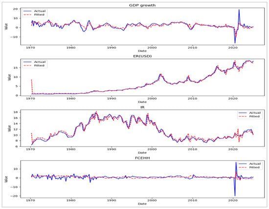
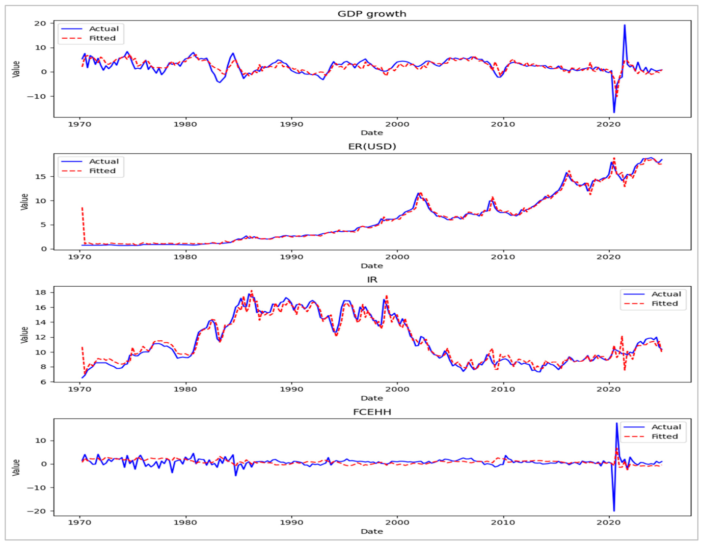
Similarly to the $VAR\left(4\right)$ model, heteroskedasticity was detected in the residuals of ER (USD) and FCEHH, but not in GDP growth rate and interest rates series based on the VARMA (1,1) model. All residuals significantly failed the Jarque–Bera test for normality, also indicating that the residuals are not normally distributed. The null hypothesis of no residual autocorrelation up to lag 10 is rejected at the 5% significance level $(p\text{-}value<0.05)$. This suggests that there is significant autocorrelation remaining in the residuals, meaning the model is not capturing all the dynamic relationships in the time series under study. The VAR (4) and VARMA (1,1) model predictions against the actual time series are presented in Figure 2 and Figure 3, respectively.

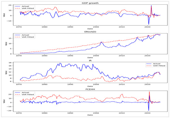
Figure 2. VAR (4) model fitted values against the actual values.

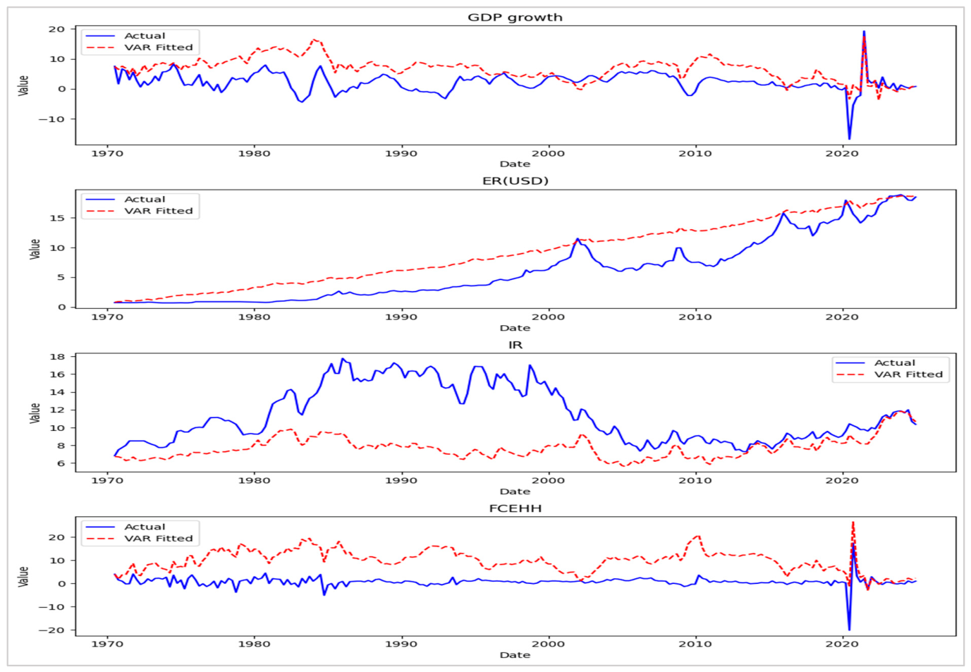
Figure 3. VARMA (1,1) model fitted values against the actual values.

Figure 2 presents the actual values of endogenous variables under study against the $VAR\left(4\right)$ model predicted in-sample values. In Figure 2, it is clear that the $VAR\left(4\right)$ model does not follow the patterns and movement of all four endogenous variables, which also shows that the $VAR\left(4\right)$ model predictions do not follow the actual values of the time series under study. In conclusion, the $VAR\left(4\right)$ model overestimated GDP growth, ER (USD) and FCEHH, but underestimated the interest rate series.

Figure 3 presents the plots of the actual values of time series under study compared to the fitted values of VARMA (1,1) model for the period of 1970:Q1 to 2024:Q4 in South Africa. It is observed from Figure 3 that the GDP growth rate and the FCEHH time series follow almost the same pattern that seem relatively correlated. In Figure 3, it is also observed that the $VARMA(1,1)$ model follows the pattern and movement of all four exogenous variables, which shows that the $VARMA(1,1)$ model predictions follow the actual values of the time series under study. The forecasting results obtained from the $VAR\left(4\right)$ and $VARMA(1,1)$ models are summarised in Table 6 and Table 7, respectively.

Table 6. Results of the VAR (4) model eight-step-ahead forecasts.

Forecasts
Yt+i	Date	GDP Growth Rate	ER (USD)	IR	FCEHH
1	31 March 2025	0.666	18.672	10.655	−0.228
2	30 June 2025	0.265	18.823	10.961	0.533
3	30 September 2025	0.839	19.012	10.968	0.909
4	31 December 2025	0.399	19.043	10.896	0.179
5	31 March 2026	0.803	19.088	10.858	0.557
6	30 June 2026	0.708	19.195	10.87	0.255
7	30 September 2026	0.233	19.285	10.912	0.411
8	31 December 2026	0.594	19.358	10.935	0.549

Table 7. Results of the VARMA (1,1) model eight-step-ahead forecasts.

Forecasts
Yt+i	Date	GDP Growth Rate	ER (USD)	IR	FCEHH
1	31 March 2025	−0.545	18.421	10.197	−0.71
2	30 June 2025	−0.282	18.101	9.809	−0.117
3	30 September 2025	−0.082	17.639	9.129	0.123
4	31 December 2025	0.139	17.291	8.692	0.232
5	31 March 2026	0.346	17.025	8.423	0.292
6	30 June 2026	0.52	16.805	8.25	0.331
7	30 September 2026	0.662	16.615	8.133	0.36
8	31 December 2026	0.777	16.445	8.055	0.382

Forecasts from the $VAR\left(4\right)$ model predict that South African GDP growth will average 0.563% from 2025:Q1 to 2026:Q4, peaking at 0.8% in Q3 2025 and Q1 2026. GDP is expected to grow by 0.2% in Q3 2026 and 0.5% in Q4 2026. Additionally, the US dollar will strengthen against the rand, climbing from R18.67/USD in 2025:Q1 to R19.36/USD by 2026:Q4. Interest rates are anticipated to average around 10.88%, rising from 10.65% to 10.94% over the same period. The FCEHH declined in 2025:Q1, then rose by an average of 0.54% from 2025:Q2 to 2025:Q4, continuing to increase by 0.44% until 2026:Q4.

The eight-step-ahead forecasts for 2025–2026 are ex ante forecasts generated from models estimated using data up to 2024:Q4. According to the results, the $VARMA(1,1)$ model projects a decline in South Africa’s GDP growth from 2025:Q1 to 2025:Q3, with a subsequent increase from 2025:Q4 to 2026:Q4, averaging 0.47% annually between 2026:Q1 and 2026:Q4. The South African rand is expected to strengthen against the US dollar, improving from R18.42/USD in 2025:Q1 to R16.45/USD by 2026:Q4. Interest rates are projected to decrease from 10.19% to 8.06% during the same period. FCEHH will rise from 2024:Q3 to 2026:Q4, despite declines in early 2024. To quantitatively assess model performance across the two statistical methods, forecast accuracy must be evaluated through actual forecasts. The residual sizes are not dependable for indicating forecast errors. Model error parameters, including Mean Absolute Error (MAE), Mean Square Error (MSE), and Root Mean Square Error (RMSE), are presented in Table 8.

Table 8. Comparison of forecasting performance of VAR (4) and VARMA (1,1) models based on in-sample fit statistics.

Model	Variables	MAE	MSE	RMSE
VAR (4)	GDP	2.475	11.973	3.460
	Exchange Rates	2.591	8.828	2.971
	Interest Rates	3.004	17.219	4.150
	FCEHH	5.945	50.369	7.097
	Overall	3.504	22.097	4.420
VARMA (1,1)	GDP	1.292	4.442	2.107
	Exchange Rates	0.402	0.567	0.753
	Interest Rates	0.550	0.571	0.756
	FCEHH	1.222	4.300	2.074
	Overall	0.867	2.470	1.423

Table 8 shows that the $VARMA(1,1)$ model outperformed the $VAR\left(4\right)$ model in predicting the time series under consideration, with the $VARMA(1,1)$ model having lower MAE, MSE, and RMSE than the $VAR\left(4\right)$ model, which had higher errors in forecasting the time series under study. In conclusion, the $VARMA(1,1$) model best predicted the South African GDP growth rate, currency rates (USD), interest rates, and final consumer expenditure by household, yielding 0.867, 2.470, and 1.423 for MAE, MSE, and RMSE, respectively. Macroeconomic and financial data exhibit volatility, trends, and seasonality, especially global oil prices, US interest rates, South African interest rates, and exchange rates. This study further employed the univariate $GARCH(1,1)$ model to assess volatility present in the dataset, and the results are presented in Appendix A.3. Given the results in Appendix A.3, the equations of $GARCH(1,1)$ model for each variable are given as follows:

$${GDP}_{{\sigma }_t^2}=0.444+{0.42ϵ}_{t-1}^2+{0.58\sigma }_{t-1}^2$$

(36)

$${ER\left(USD\right)}_{{\sigma }_t^2}=0.0001+{0.121ϵ}_{t-1}^2+{0.879\sigma }_{t-1}^2$$

(37)

$${IR}_{{\sigma }_t^2}=0.011+{0.079ϵ}_{t-1}^2+{0.901\sigma }_{t-1}^2$$

(38)

$$FCEHH=3.739+{0.465ϵ}_{t-1}^2+{0.0001\sigma }_{t-1}^2$$

(39)

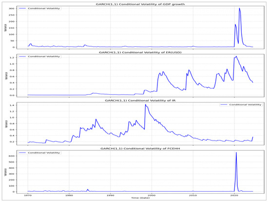
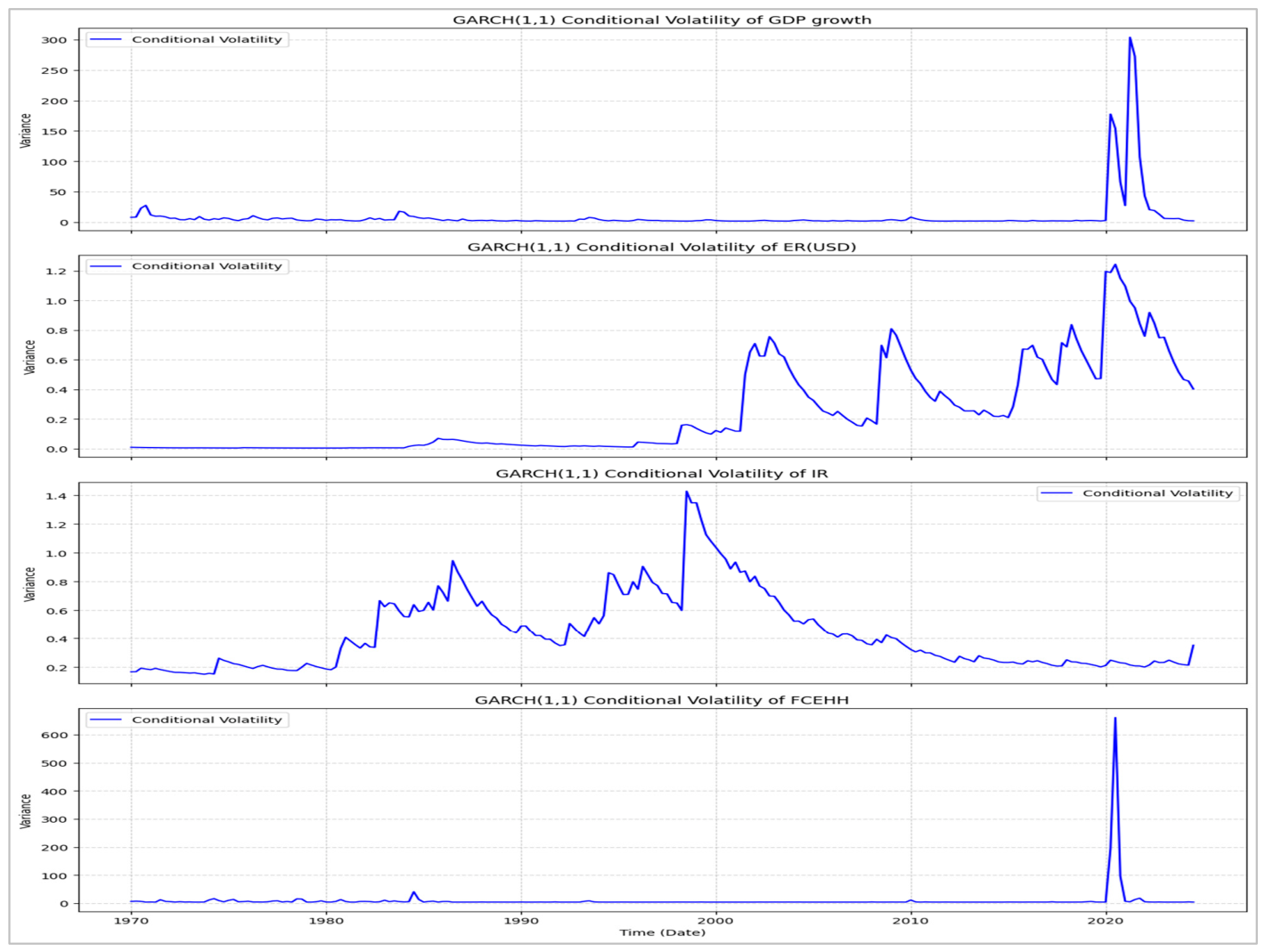
The results from $GARCH(1,1)$ model indicate that the GDP growth model exhibits a persistence parameter of $(\alpha +\beta =1)$, suggesting an IGARCH-type process rather than a stationary GARCH process. This implies that volatility shocks to GDP growth are highly persistent and their effects do not dissipate over time. Additionally, the conditional variance is low and insignificant, suggesting low volatility in the GDP growth series. The GARCH model for the USD exchange rate indicates persistent volatility shocks $(\alpha +\beta \approx 1)$ and a low, insignificant conditional variance parameter (omega), suggesting a long-lasting impact on future volatility. Furthermore, the $GARCH(1,1)$ model indicates that volatility shocks have a long-lasting impact on interest rates, as the persistence parameter is near 1. Additionally, the interest rates series exhibits low insignificant volatility, with a conditional variance of 0.011. The estimated $GARCH(1,1$) model for FCEHH indicates that the ARCH coefficient is positive and statistically significant at the 10% level, suggesting weak evidence that current volatility is influenced by recent shocks. However, the GARCH coefficient is statistically insignificant and economically negligible, indicating that past conditional volatility does not significantly affect current volatility. Consequently, FCEHH volatility appears to be driven primarily by short-term shocks with no evidence of volatility persistence, implying that the estimated $GARCH(1,1)$ model effectively behaves as an $ARCH\left(1\right)$ process. Figure 4 presents the conditional volatility analysis.

Figure 4. Conditional volatility analysis of variables under study.

Figure 4 illustrates the forecasted conditional volatility of the GDP growth rate, indicating moderate volatility from the 1970s to the 1990s, followed by low volatility from 2000 to 2020. Notably, from 2020 to 2023, the South African GDP growth rate exhibited high volatility attributed to the COVID-19 pandemic. In terms of the exchange rate (ER) against the USD, Figure 4 shows moderate constancy from 1970 to 1985, with irregular fluctuations and increasing volatility from the late 1980s, reflecting sensitivity to external economic changes. The interest rate in South Africa showed high volatility from the 1970s until the 2000s, after which it declined and stabilised at lower levels post-2010. The interest rate was highly responsive to economic development until the 2000s, then became less reactive. The FCEHH conditional volatility, also shown in Figure 4, was moderate between the 1970s and 1980s, dropping in the 1990s, aside from a shock in 1994 linked to governmental transitions. Further shocks occurred around 2010 due to the global recession, and heightened volatility was observed from 2020 to 2022 due to the global health crisis. Figure 5 presents the conditional volatility from the $GARCH(1,1)$ model.

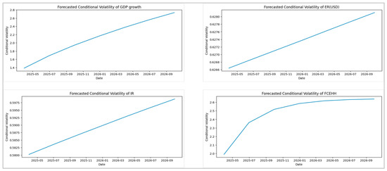
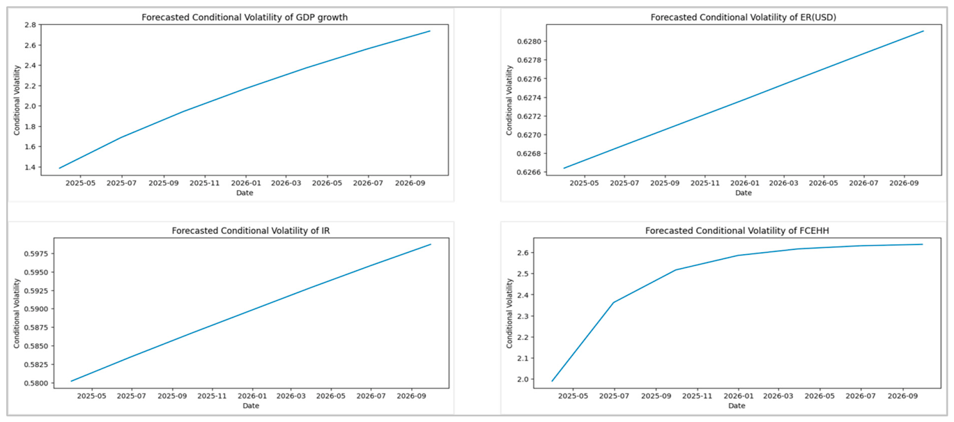
Figure 5. Conditional volatility forecast results from GARCH (1,1) model.

Figure 5 presents the forecasted conditional volatility of GDP growth rate, ER (USD), interest rates and FCEHH. It is clear from Figure 5 that the GARCH model forecasted increasing volatility for all the time series under study, as the forecasted volatility graphs show an increasing trend over the period of 2025:Q1 to 2026:Q4. In addition, the GARCH-forecasted volatility for the GDP growth rate, ER (USD) and interest rates show a similar direct relationship, whilst the FCEHH volatility series increases between 2025:Q1 and 2026:Q1; however, it will remain steady over the last three quarters of 2026. In summary, the forecasted volatility signals the risk and potential of new trends in either direction. Given the evidence of persistent volatility and the potential presence of asymmetric effects, the EGARCH and GJR-GARCH models were subsequently estimated to assess whether positive and negative shocks exert different impacts on volatility.

Table 9 presents the results of the $EGARCH(1,1)$ and $GJR-GARCH(1,1)$ models for GDP growth, the ZAR/USD exchange rate, interest rates, and FCEHH. The EGARCH results indicate significant volatility persistence across most series, particularly for the exchange rate, GDP growth, and interest rates. Evidence of asymmetric volatility is observed only for the interest rate series, where the asymmetry parameter is positive and statistically significant, suggesting that positive and negative shocks have different effects on future volatility. In contrast, the asymmetry parameters for GDP growth, the exchange rate, and FCEHH are statistically insignificant, indicating no significant leverage effects.

Table 9. Parameters of asymmetric GARCH models.

EGARCH (1,1)
Parameters	GDP growth	ER (USD)	IR	FCEHH
Omega	0.298 (0.026)	−0.255 (0.025)	−0.057 (0.485)	0.546 (0.620)
Alpha	1.178 (0.0001)	3.049 (0.0001)	1.968 (0.0001)	1.161 (0.177)
Gamma	−0.085 (0.275)	0.079 (0.388)	0.342 (0.0001)	0.6765 (0.723)
Beta	0.804 (0.0001)	0.911 (0.0001)	0.748 (0.0001)	0.047 (0.0001)
GJR-GARCH (1,1)
Parameters	GDP growth	ER (USD)	IR	FCEHH
Omega	0.616 (0.041)	0.021 (0.765)	0.141 (0.008)	0.169 (0.135)
Alpha	0.605 (0.0001)	1.000 (0.565)	1.000 (0.0001)	0.538 (0.0001)
Gamma	0.253 (0.089)	−0.119 (0.066)	−0.114 (0.440)	−0.007 (0.973)
Beta	0.269 (0.0001)	0.032 (0.986)	0.001 (1.000)	0.465 (0.0001)

The $GJR-GARCH(1,1)$ results provide limited support for asymmetric volatility behaviour. The leverage parameter is statistically insignificant for all variables at the 5% significance level, implying that negative shocks do not exert a significantly different impact on volatility compared to positive shocks of the same magnitude. Overall, the findings suggest that volatility persistence is a dominant feature of the series, while asymmetric effects are largely absent, except for the interest rate series under the EGARCH specification. These results further indicate that the EGARCH model captures asymmetry more effectively than the GJR-GARCH model for the data under consideration. Following the estimation of the $EGARCH(1,1)$ and $GJR-GARCH(1,1)$ models, diagnostic tests were conducted on the standardised residuals to assess model adequacy.

Table 10 and Table 11 present the Ljung–Box diagnostic test results for the standardised residuals and squared standardised residuals of the $EGARCH(1,1)$ and $GJR-GARCH(1,1)$ models. For both models, the GDP growth, exchange rate, and interest rate series exhibit statistically significant Ljung–Box statistics for the standardised residuals (p < 0.001), indicating the presence of residual autocorrelation. This suggests that the models do not fully capture the serial dependence structure of these series and that some information remains unexplained. In contrast, the FCEHH series shows insignificant Ljung–Box statistics (p > 0.05), implying that the residuals behave as white noise and that the fitted models adequately capture the underlying dynamics.

Table 10. Ljung–Box test of autocorrelation for $EGARCH(1,1$) model.

Ljung–Box Test of Autocorrelation
Test		GDP Growth	ER (USD)	IR	FCEHH
Test on standardised residuals (Autocorrelation)	t-statistic	156.066	1648.221	1103.611	4.791
	p-value	<0.0001	<0.0001	<0.0001	0.905
Test on standardised residuals (ARCH effects)	t-statistic	1.494	23.576	8.905	0.095
	p-value	1.000	0.009	0.541	1.000

Table 11. Ljung–Box test of autocorrelation for $GJR-GARCH(1,1)$ model.

Ljung–Box Test of Autocorrelation
Test		GDP Growth	ER (USD)	IR	FCEHH
Test on standardised residuals (Autocorrelation)	t-statistic	157.362	1821.099	1014.652	3.152
	p-value	<0.0001	<0.0001	<0.0001	0.978
Test on standardised residuals (ARCH effects)	t-statistic	2.872	25.602	11.362	0.082
	p-value	0.984	0.004	0.330	1.000

The Ljung–Box tests applied to the squared standardised residuals reveal no remaining ARCH effects for GDP growth, interest rates, and FCEHH under both model specifications, as evidenced by the insignificant p-values. However, the exchange rate series exhibits significant ARCH effects under both the $EGARCH(1,1)$ and $GJR-GARCH(1,1)$ models, indicating that residual heteroskedasticity remains present. This suggests that neither asymmetric GARCH specification fully captures the volatility dynamics of the exchange rate series. Overall, the diagnostic results indicate that the $EGARCH(1,1)$ and $GJR-GARCH(1,1)$ models provide an adequate fit for FCEHH and effectively remove conditional heteroskedasticity from most series, but they fail to eliminate residual autocorrelation in GDP growth, exchange rates, and interest rates, while also leaving significant ARCH effects in the exchange rate series. To address this misspecification, this study further refined the EGARCH and GJR-GARCH models to incorporate the ARMA terms into the mean equations to see if it significantly improves the residual diagnostics.

Table 12 presents the results of the $EGARCH(1,1)-ARMA(1,1)$ and $GJR-GARCH(1,1)-ARMA(1,1)$ models. The findings indicate that volatility persistence remains a prominent feature across all variables, particularly for the exchange rate and interest rate series, where the persistence parameters are close to unity. The EGARCH-ARMA model identifies a significant asymmetric effect only for the interest rate series, while the GJR-GARCH-ARMA model detects asymmetry only in the exchange rate series. No significant leverage effects are observed for GDP growth or FCEHH under either specification. Overall, the results suggest that incorporating ARMA terms improves the modelling of the conditional mean while preserving the strong volatility persistence observed in the series. However, evidence of asymmetric volatility remains limited and is dependent on the chosen model specification.

Table 12. Parameters of asymmetric GARCH models with an ARMA mean.

EGARCH (1,1) − ARMA (1,1)
Parameters	GDP Growth	ER (USD)	IR	FCEHH
Omega	0.076 (0.388)	0.366 (0.563)	−0.014 (0.0001)	2.590 (0.0001)
Alpha	0.539 (0.004)	0.605 (0.477)	−0.103 (0.0001)	3.130 (0.0001)
Gamma	0.016 (0.873)	0.768 (0.326)	0.047 (0.0001)	−0.331 (0.428)
Beta	0.881 (0.0001)	0.998 (0.0001)	0.995 (0.0001)	0.746 (0.0001)
GJR-GARCH (1,1) − ARMA (1,1)
Parameters	GDP growth	ER (USD)	IR	FCEHH
Omega	0.183 (0.064)	0.0001 (0.532)	0.007 (0.168)	0.169 (0.113)
Alpha	0.463 (0.042)	0.282 (0.003)	0.074 (0.088)	0.390 (0.021)
Gamma	0.082 (0.745)	−0.282 (0.001)	−0.026 (0.846)	0.215 (0.424)
Beta	0.497 (0.0001)	0.859 (0.0001)	0.929 (0.0001)	0.502 (0.0001)

Table 13 and Table 14 present the Ljung–Box diagnostic test results for the $EGARCH-ARMA(1,1)$ and $GJR-GARCH-ARMA(1,1)$ models. The results indicate a substantial improvement in model adequacy following the inclusion of ARMA terms in the mean equation. For both model specifications, the Ljung–Box tests on the standardised residuals are statistically insignificant across all variables, suggesting the absence of residual autocorrelation and indicating that the models adequately capture the serial dependence structure of the data. Similarly, the Ljung–Box tests on the squared standardised residuals are insignificant, implying that no remaining ARCH effects are present and that the conditional heteroskedasticity has been successfully modelled. Overall, the diagnostic results demonstrate that the $EGARCH-ARMA(1,1)$ and $GJR-GARCH-ARMA(1,1)$ models produce residuals that closely resemble white noise, confirming that the inclusion of ARMA terms effectively resolves the misspecification detected in the original asymmetric GARCH models and provides a more adequate representation of the underlying volatility dynamics.

Table 13. Ljung–Box test of autocorrelation for EGARCH − ARMA (1,1) model.

Ljung–Box Test of Autocorrelation
Test		GDP Growth	ER (USD)	IR	FCEHH
Test on standardised residuals (Autocorrelation)	t-statistic	17.982	21.197	15.6	3.671
	p-value	0.055	0.097	0.112	0.961
Test on standardised residuals (ARCH effects)	t-statistic	0.099	8.186	10.85	0.11
	p-value	1.000	0.611	0.369	1.000

Table 14. Ljung–Box test of autocorrelation for GJR − GARCH − ARMA (1,1) model.

Ljung–Box Test of Autocorrelation
Test		GDP Growth	ER (USD)	IR	FCEHH
Test on standardised residuals (Autocorrelation)	t-statistic	14.256	15.463	11.061	4.663
	p-value	0.162	0.116	0.353	0.912
Test on standardised residuals (ARCH effects)	t-statistic	0.103	16.025	11.252	0.093
	p-value	1.000	0.099	0.338	1.000

5. Conclusions and Recommendations

This study examined South African macroeconomic and financial time series using VAR, VARMA, and GARCH frameworks based on quarterly data spanning 1970:Q1 to 2024:Q4. Model estimation and evaluation were conducted at the 5% significance level. The diagnostic results indicate that the $VAR\left(4\right)$ model does not adequately capture the underlying dynamics of the series. This finding is consistent with the broader literature, as [32] has shown that even small departures from correct VAR specification can significantly distort inference and impulse responses, highlighting the sensitivity of VAR models to misspecification. In particular, the presence of heteroskedasticity in ER (USD) and FCEHH, the consistent rejection of residual normality, and significant autocorrelation as revealed by the Portmanteau test point to model misspecification and unaccounted higher-order or nonlinear dynamics. These shortcomings suggest the need for further refinement, including the exploration of higher lag structures and the incorporation of relevant exogenous variables.

Similarly, the $VARMA(1,1)$ model does not yield a meaningful improvement in residual diagnostics relative to the $VAR\left(4\right)$ specification. This finding is consistent with recent literature by [9], who indicated that VARMA models often provide limited empirical advantages over VAR models because of identification and estimation challenges. Furthermore, ref. [10] noted that VARMA models may barely show any advantage over VARs in finite samples. This reinforces the view that both VAR and VARMA models may be insufficient to capture the complexity of the underlying data-generating process. As such, alternative modelling approaches incorporating different lag structures, seasonal components, and more flexible multivariate frameworks should be considered. This study then employed the GARCH model. In contrast to the findings from VAR and VARMA, the $GARCH(1,1)$ model provided useful insights into the volatility dynamics of the series. It effectively captures time-varying volatility and persistence in GDP growth, with conditional variance reflecting periods of economic expansion and contraction. The findings align with recent studies, such as [17,20], which highlighted that GARCH-type models are effective in modelling volatility clustering and persistent macroeconomic shocks. Additionally, studies such as [19] demonstrated that GARCH-type frameworks effectively extract time-varying volatility and capture periods of heightened economic uncertainty through volatility clustering and macroeconomic uncertainty effects.

For ER (USD), the model successfully identifies volatility clustering, while for FCEHH, the near unity sum of parameters indicates high persistence in volatility. However, the insignificance of individual parameters in the FCEHH model suggests that the standard $GARCH(1,1)$ specification may be inadequate for this series. Overall, the findings revealed distinct volatility patterns across variables: ER (USD) and FCEHH exhibit highly persistent volatility, whereas GDP growth demonstrates mean-reverting behaviour, similar to the study conducted by [20]. While GARCH models account for conditional heteroskedasticity, they do not fully address non-normality in residuals, indicating the need for more flexible volatility specifications, such as EGARCH and GJR-GARCH.

The findings suggest that forecasting performance may benefit from accounting for both mean dynamics and volatility characteristics. In the forecasting analysis, the exchange rate projections from the $VAR\left(4\right)$ and $VARMA(1,1)$ models diverge notably, with $VAR\left(4\right)$ indicating a depreciation path, while $VARMA(1,1)$ suggests an appreciation. This divergence arises from the different dynamic structures of the two models. As a purely autoregressive specification, the $VAR\left(4\right)$ model tends to propagate past shocks and trends, resulting in a more persistent depreciation path. In contrast, the $VARMA(1,1)$ model incorporates a moving-average component that accounts for past innovations and dampens the persistence of shocks, thereby inducing a degree of mean reversion and yielding an appreciation path. Economically, the contrasting forecasts suggest that exchange rate projections are sensitive to model specification and underlying assumptions regarding shock persistence and adjustment dynamics. The divergence therefore highlights the importance of considering multiple modelling frameworks when evaluating future exchange rate movements and interpreting forecast uncertainty in macroeconomic and financial time series.

These findings have important implications for economic policy and forecasting in South Africa. The persistence of volatility, particularly in exchange rates and interest rates, suggests that economic shocks can have prolonged effects, increasing uncertainty for investment, trade, and policy planning. Exchange rate volatility may elevate risks associated with international transactions, while fluctuations in household consumption can influence aggregate demand and economic growth. The results also demonstrate that accounting for volatility clustering and asymmetric responses provides a more comprehensive understanding of macroeconomic dynamics than linear models alone. Consequently, policymakers and analysts should incorporate nonlinear volatility models into forecasting and policy evaluation frameworks to better manage economic risks and improve decision-making in an uncertain economic environment.

This study is, however, subject to several limitations. Cointegration analysis was not undertaken to examine the existence of long-run equilibrium relationships among the variables. The analysis focused exclusively on short-run dynamics and predictive accuracy. The use of linear VAR and VARMA models may not fully capture nonlinear dynamics, while the findings demonstrate the usefulness of VARMA and asymmetric GARCH models in capturing the interrelationships and volatility dynamics among GDP growth, exchange rates, interest rates, and household consumption expenditure. Several limitations should be acknowledged. The initial VAR and VARMA specifications assume linear relationships and may not fully capture potential nonlinear interactions among the macroeconomic variables. Although this study extended the volatility analysis by employing EGARCH and GJR-GARCH models with ARMA mean specifications, other forms of nonlinearity and regime-dependent behaviour may remain unaccounted for. The evidence of highly persistent volatility, particularly in the exchange rate and interest rate series, suggests that alternative nonlinear approaches, such as Markov-switching, threshold, or machine learning-based models, may provide additional insights.

Furthermore, the estimated models rely on fixed lag structures and exclude potentially important exogenous variables, such as monetary policy shocks, global economic conditions, commodity prices, and geopolitical events, which may influence both the conditional mean and variance processes. The long sample period may also encompass structural breaks associated with major economic events, including the global financial crisis, the COVID-19 pandemic, and domestic policy changes, which could affect parameter stability and forecasting performance. In addition, the use of aggregated quarterly data may mask short-term fluctuations and volatility dynamics that could be captured using higher-frequency observations. A further limitation relates to forecast evaluation. Although the study generated multi-step-ahead forecasts and compared model performance using forecast error measures, realised observations beyond 2024 were unavailable at the time of analysis. Consequently, the reported forecasts could not be subjected to a formal out-of-sample validation using actual observed values. Future research should therefore employ rolling-window, recursive, or holdout-sample validation frameworks once additional observations become available. Such approaches would provide a more rigorous assessment of forecasting accuracy and model stability over time. Future studies may also consider incorporating exogenous variables, structural break adjustments, nonlinear multivariate models, and higher-frequency data to further improve forecasting performance and enhance understanding of South Africa’s macroeconomic dynamics. Future studies may extend the present work by formally testing for cointegration and comparing the forecasting performance of VECM-based specifications with the VAR/VARMA models considered in this study. From a policy perspective, adopting adaptive and forward-looking analytical frameworks will be essential for effectively managing volatility, reducing uncertainty, and supporting sustainable economic growth in South Africa.

Appendix A.1. Parameter Estimation Results of the VAR (4) Model

Model	Parameters	Coefficient	Std Error	t-Stat	p-Value
GDP	Const	0.101	0.126	0.797	0.425
	GDPt-1	−0.14	0.097	−1.442	0.149
	ERt-1	−1.524	0.263	−5.798	0.0001 ***
	IRt-1	−0.255	0.205	−1.244	0.214
	FCEHHt-1	0.033	0.086	0.386	0.7
	GDPt-2	−0.063	0.058	−1.088	0.277
	ERt-2	0.184	0.308	0.598	0.55
	IRt-2	0.033	0.212	0.158	0.875
	FCEHHt-2	0.176	0.108	1.625	0.104
	GDPt-3	−0.036	0.058	−0.611	0.541
	ERt-3	−0.015	0.309	−0.048	0.962
	IRt-3	−0.089	0.212	−0.419	0.675
	FCEHHt-3	0.362	0.108	3.338	0.001 ***
	GDPt-4	−0.292	0.057	−5.104	0.0001 ***
	ERt-4	−0.024	0.296	−0.083	0.934
	IRt-4	−0.538	0.199	−2.705	0.007 ***
	FCEHHt-4	−0.076	0.091	−0.837	0.403
ER (USD)	Const	0.071	0.034	2.048	0.041.
	GDPt-1	0.007	0.026	0.252	0.801
	ERt-1	0.292	0.072	4.068	0.0001 ***
	IRt-1	0.055	0.056	0.978	0.328
	FCEHHt-1	−0.007	0.024	−0.316	0.752
	GDPt-2	−0.007	0.016	−0.464	0.642
	ERt-2	−0.211	0.084	−2.501	0.012 ***
	IRt-2	−0.038	0.058	−0.649	0.516
	FCEHHt-2	0.009	0.03	0.301	0.763
	GDPt-3	0.003	0.016	0.185	0.853
	ERt-3	0.162	0.085	1.919	0.055.
	IRt-3	−0.077	0.058	−1.325	0.185
	FCEHHt-3	0.033	0.03	1.106	0.269
	GDPt-4	0.027	0.016	1.745	0.081
	ERt-4	−0.06	0.081	−0.745	0.456
	IRt-4	0.015	0.054	0.268	0.789
	FCEHHt-4	0.004	0.025	0.179	0.858
IR	Const	−0.013	0.044	−0.284	0.776
	GDPt-1	0.015	0.034	0.443	0.658
	ERt-1	0.414	0.093	4.47	0.0001 ***
	IRt-1	0.22	0.072	3.041	0.002 *
	FCEHHt-1	−0.011	0.03	−0.347	0.729
	GDPt-2	0.001	0.02	0.058	0.954
	ERt-2	−0.075	0.109	−0.689	0.491
	IRt-2	−0.134	0.075	−1.792	0.073
	FCEHHt-2	−0.024	0.038	−0.622	0.534
	GDPt-3	−0.008	0.021	−0.367	0.713
	ERt-3	−0.004	0.109	−0.041	0.968
	IRt-3	−0.114	0.075	−1.521	0.128
	FCEHHt-3	−0.016	0.038	−0.43	0.667
	GDPt-4	0.005	0.02	0.264	0.792
	ERt-4	−0.037	0.104	−0.354	0.723
	IRt-4	0.085	0.07	1.217	0.224
	FCEHHt-4	−0.023	0.032	−0.712	0.476
FCEHH	Const	0.157	0.145	1.079	0.281
	GDPt-1	0.023	0.112	0.207	0.836
	ERt-1	−1.992	0.303	−6.579	0.0001 ***
	IRt-1	−0.542	0.236	−2.294	0.022 *
	FCEHHt-1	−1.19	0.1	−11.95	0.0001 ***
	GDPt-2	−0.197	0.067	−2.947	0.003 *
	ERt-2	0.393	0.355	1.107	0.268
	IRt-2	−0.038	0.244	−0.157	0.875
	FCEHHt-2	−0.985	0.125	−7.914	0.0001 ***
	GDPt-3	−0.187	0.067	−2.794	0.005 *
	ERt-3	−0.106	0.356	−0.298	0.766
	IRt-3	−0.012	0.244	−0.049	0.961
	FCEHHt-3	−0.678	0.125	−5.427	0.0001 ***
	GDPt-4	−0.155	0.066	−2.347	0.01 **
	ERt-4	−0.298	0.341	−0.873	0.383
	IRt-4	−0.442	0.229	−1.928	0.054.
	FCEHHt-4	−0.353	0.104	−3.382	0.001 **
Significance codes: 0 ‘***’ 0.001 ‘**’ 0.01 ‘*’ 0.05 ‘.’ 0.1 ‘ ’ 1

Appendix A.2. Parameter Estimation Results of the VARMA (1,1) Model

Model	Parameters	Coefficient	Std Error	t-Stat	p-Value
GDP growth	Constant	2.6644	5.637	0.473	0.636
	GDPt-1	0.6137	0.288	2.13	<0.033 *
	ERt-1	−0.0856	0.174	−0.492	0.623
	IRt-1	−0.105	0.3	−0.349	0.727
	FCEHHt-1	−0.0498	0.713	−0.07	0.944
	GDP-MAt-1	−0.2525	0.302	−0.838	0.402
	ER-MAt-1	−1.1745	0.329	−3.574	<0.0001 ***
	IR-MAt-1	−0.9679	0.421	−2.298	<0.022 *
	FCEHH-MAt-1	0.3776	0.683	0.553	0.58
ER (USD)	Constant	4.8389	4.422	1.094	0.274
	GDPt-1	−0.1986	0.232	−0.854	0.393
	ERt-1	0.8454	0.136	6.204	<0.0001 ***
	IRt-1	−0.2657	0.241	−1.105	0.269
	FCEHHt-1	−0.4092	0.514	−0.796	0.426
	GDP-MAt-1	0.2036	0.234	0.871	0.384
	ER-MAt-1	0.5455	0.192	2.845	<0.004 **
	IR-MAt-1	0.3714	0.288	1.29	0.197
	FCEHH-MAt-1	0.4369	0.542	0.806	0.42
Interest Rate	Constant	10.1487	8.067	1.258	0.208
	GDPt-1	−0.431	0.422	−1.022	0.307
	ERt-1	−0.2976	0.243	−1.223	0.221
	IRt-1	0.4229	0.438	0.965	0.335
	FCEHHt-1	−0.8395	0.931	−0.902	0.367
	GDP-MAt-1	0.4076	0.414	0.986	0.324
	ER-MAt-1	0.7918	0.296	2.671	<0.008 **
	IR-MAt-1	0.9385	0.459	2.046	<0.041 *
	FCEHH-MAt-1	0.8587	0.93	0.923	0.356
FCEHH	Constant	0.4578	4.372	0.105	0.917
	GDPt-1	0.0612	0.21	0.291	0.771
	ERt-1	−0.013	0.133	−0.097	0.923
	IRt-1	−0.0041	0.225	−0.018	0.985
	FCEHHt-1	0.3679	0.659	0.558	0.577
	GDPMAt-1	−0.1837	0.243	−0.755	0.450
	ERMAt-1	−0.3068	0.293	−1.049	0.294
	IR-MAt-1	−0.4102	0.258	−1.593	0.111.
	FCEHH-MAt-1	−0.5958	0.623	−0.956	0.339
Significance codes: 0 ‘***’ 0.001 ‘**’ 0.01 ‘*’ 0.05 ‘.’ 0.1 ‘ ’ 1

Appendix A.3. Parameter Estimation Results of the GARCH (1,1) Model

GARCH (1,1) GDP growth rate model
Mean Model
Parameter		coefficient		std. error		t-statistic	p-value
Mu		−0.211		0.166		−1.268	0.205
Volatility Model
		coefficient		std. error		t-statistic	p-value
Omega		0.4439		0.855		0.519	0.604
alpha [1]		0.42		0.236		1.782	<0.075
beta [1]		0.58		0.207		2.808	<0.005
GARCH (1,1) ER (USD) model
Mean Model
Parameters	Coefficient		std. error			t-statistic	p-value
Mu	0.008		0.011			0.761	0.446
Volatility Model
Parameters	Coefficient		std. error			t-statistic	p-value
Omega	0.000		0.001			0.361	0.718
alpha [1]	0.121		0.123			0.985	0.325
beta [1]	0.879		0.198			4.450	<0.0001
GARCH (1,1) interest rates model
Mean Model
Parameters	Coefficient			std. error	t-statistic		p-value
Mu	0.048			0.041	1.163		0.245
Volatility Model
Parameters	Coefficient			std. error	t-statistic		p-value
Omega	0.011			0.007	1.496		0.135
alpha [1]	0.079			0.029	2.696		<0.007
beta [1]	0.901			0.022	40.501		<0.0001
GARCH (1,1) FCEHH model
Mean Model
Parameters	Coefficient		std. error			t-statistic	p-value
Mu	−0.081		0.105			−0.772	0.440
Volatility Model
Parameters	Coefficient		std. error			t-statistic	p-value
Omega	3.739		2.632			1.421	0.155
alpha [1]	0.465		0.251			1.852	0.064
beta [1]	0.0001		0.126			0.000	1.000

References

- Lütkepohl, H. Introduction to Multiple Time Series Analysis; Springer Science & Business Media: Berlin/Heidelberg, Germany, 2013. [Google Scholar]
- Tsay, R.S. Multivariate Time Series Analysis: With R and Financial Applications; John Wiley & Sons: Hoboken, NJ, USA, 2013. [Google Scholar]
- Athanasopoulos, G.; Vahid, F. VARMA versus VAR for Macroeconomic Forecasting. J. Bus. Econ. Stat. 2008, 26, 237–252. [Google Scholar] [CrossRef] [Scilit]
- Ogbuabor, J.E.; Malaolu, V.A.; Orji, A. Asymmetric Effects of Policy Uncertainty on Real Sector Variables in Emerging Markets: Evidence from Brazil, India, China and South Africa. Int. J. Emerg. Mark. 2024, 19, 2070–2090. [Google Scholar]
- Ndou, E.; Gumata, N.; Ncube, M. Global Economic Uncertainties and Exchange Rate Shocks: Transmission Channels to the South African Economy; Springer: Berlin/Heidelberg, Germany, 2018. [Google Scholar]
- Ding, J.; Tarokh, V.; Yang, Y. Model Selection Techniques: An Overview. IEEE Signal Process. Mag. 2018, 35, 16–34. [Google Scholar] [CrossRef] [Scilit]
- Simionescu, M. The Use of VARMA Models in Forecasting Macroeconomic Indicators. Econ. Sociol. 2013, 6, 94–102. [Google Scholar] [CrossRef] [Scilit]
- Russel, E.; Usman, M. Vector Autoregressive with Exogenous Variable Model and Its Application in Modeling and Forecasting Energy Data: Case Study of PTBA and HRUM Energy. Int. J. Energy Econ. Policy 2019, 9, 390–398. [Google Scholar] [CrossRef] [Scilit]
- Düker, M.; Matteson, D.S.; Tsay, R.S.; Wilms, I. Vector Autoregressive Moving Average Models: A Review. WIREs Comput. Stat. 2025, 17, e70009. [Google Scholar] [CrossRef] [Scilit] [PubMed]
- Yao, W.; Kam, T.; Vahid, F. On Weak Identification in Structural VARMA Models. Econ. Lett. 2017, 156, 1–6. [Google Scholar] [CrossRef] [Scilit]
- Ali, S. Modeling and Forecasting Inflation in Ethiopia Using Multivariate Time Series Analysis. Econ. Bus. J. ECBIS 2024, 2, 395–404. [Google Scholar] [CrossRef] [Scilit]
- Majenge, L.; Mpungose, S.; Msomi, S. Comparative Analysis of VAR and SVAR Models in Assessing Oil Price Shocks and Exchange Rate Transmission to Consumer Prices in South Africa. Econometrics 2025, 13, 8. [Google Scholar] [CrossRef] [Scilit]
- Dufour, J.-M.; Pelletier, D. Practical Methods for Modelling Weak VARMA Processes: Identification, Estimation and Specification with a Macroeconomic Application. McGill Univ. Dep. Econ. CIREQ CIRANO Discuss. Pap. 2008. [Google Scholar]
- Becker, M. Varma Versus Steady-State Bvar for Macroeconomic Forecasting. Master’s Thesis, Uppsala University, Uppsala, Sweden, 2025. [Google Scholar]
- Osolo, M.O.; Okoli, C.N.; Laisin, M.S. Time-Varying Scalar Component VARMA: A State-Space Solution to Structural Instability in Macroeconomic Forecasting. Asian J. Math. Comput. Res. 2026, 33, 43–54. [Google Scholar]
- Sekati, B.N.Y.; Tsoku, J.T.; Metsileng, L.D. Modelling the Oil Price Volatility and Macroeconomic Variables in South Africa Using the Symmetric and Asymmetric GARCH Models. Cogent Econ. Financ. 2020, 8, 1792153. [Google Scholar] [CrossRef] [Scilit]
- Mohammadi, H.; Su, L. International Evidence on Crude Oil Price Dynamics: Applications of ARIMA-GARCH Models. Energy Econ. 2010, 32, 1001–1008. [Google Scholar] [CrossRef] [Scilit]
- Wang, Z.; Xing, T.; Wang, X. Economic Uncertainty and Stock Market Asymmetric Volatility: Analysis Based on the Asymmetric GARCH-MIDAS Model. Int. J. Emerg. Mark. 2025, 20, 3488–3511. [Google Scholar]
- Asri, M. Macroeconomic Volatility and Forecasting Growth in Developing Asia: An EViews GARCH-EGARCH Approach. Res. Sq. 2025. [Google Scholar] [CrossRef] [Scilit] [PubMed]
- Bouzid, K.N.; Makala, U.E. Casablanca Stock Exchange Response to the COVID-19 Pandemic. Afr. Rev. Econ. Financ. 2021, 13, 142–167. [Google Scholar]
- Alam, M.S.; Amendola, A.; Candila, V.; Jabarabadi, S.D. Is Monetary Policy a Driver of Cryptocurrencies? Evidence from a Structural Break Garch-Midas Approach. Econometrics 2024, 12, 2. [Google Scholar] [CrossRef] [Scilit]
- Kalsie, A.; Arora, A. Structural Break, US Financial Crisis and Macroeconomic Time Series: Evidence from BRICS Economies. Transnatl. Corp. Rev. 2019, 11, 250–264. [Google Scholar] [CrossRef] [Scilit]
- Viegi, N. Introduction to VAR Models; University of Pretoria: Pretoria, South Africa, 2010. [Google Scholar]
- Elias, I.I.; Ali, T.H. VARMA Time Series Model Analysis Using Discrete Wavelet Transformation Coefficients for Coiflets Wavelet. Passer J. Basic Appl. Sci. 2025, 7, 657–677. [Google Scholar] [CrossRef] [Scilit]
- Dias, G.F.; Kapetanios, G. Estimation and Forecasting in Vector Autoregressive Moving Average Models for Rich Datasets. J. Econom. 2018, 202, 75–91. [Google Scholar] [CrossRef] [Scilit]
- Engle, R.F. Autoregressive Conditional Heteroscedasticity with Estimates of the Variance of United Kingdom Inflation. Econom. J. Econom. Soc. 1982, 50, 987–1007. [Google Scholar] [CrossRef] [Scilit]
- Bollerslev, T. A Conditionally Heteroskedastic Time Series Model for Speculative Prices and Rates of Return. Rev. Econ. Stat. 1987, 69, 542–547. [Google Scholar] [CrossRef] [Scilit]
- Shamiri, A.; Hassan, A. Modeling and Forecasting Volatility of the Malaysian and the Singaporean Stock Indices Using Asymmetric GARCH Models and Non-Normal Densities. J. Malays. Math. Sci. 2007, 1, 83–102. [Google Scholar]
- Ali, G. EGARCH, GJR-GARCH, TGARCH, AVGARCH, NGARCH, IGARCH and APARCH Models for Pathogens at Marine Recreational Sites. J. Stat. Econom. Methods 2013, 2, 57–73. [Google Scholar]
- Lütkepohl, H. Estimation of Vector Autoregressive Processes. In New Introduction to Multiple Time Series Analysis; Springer: Berlin/Heidelberg, Germany, 2005; pp. 69–133. [Google Scholar]
- Enders, W. Applied Econometric Time Series; Wiley: Hoboken, NJ, USA, 2015. [Google Scholar]
- Olea, J.L.M.; Plagborg-Møller, M.; Qian, E.; Wolf, C.K. Double Robustness of Local Projections and Some Unpleasant Varithmetic; National Bureau of Economic Research: New York, NY, USA, 2024. [Google Scholar]
Disclaimer/Publisher’s Note: The statements, opinions and data contained in all publications are solely those of the individual author(s) and contributor(s) and not of MDPI and/or the editor(s). MDPI and/or the editor(s) disclaim responsibility for any injury to people or property resulting from any ideas, methods, instructions or products referred to in the content. |
© 2026 by the authors. Licensee MDPI, Basel, Switzerland. This article is an open access article distributed under the terms and conditions of the Creative Commons Attribution (CC BY) license.