Viscous Current Induced by Kelvin Force in Ordinary Fluids with Magnetic Susceptibility Contrasts

Abstract

The magnetic susceptibilities of various electrically insulating ordinary fluids depend on their local states, such as their density and temperature. When such fluids, which can be characterized as either paramagnetic or diamagnetic and occur commonly in nature, are subjected to magnetic field gradients, it induces an effective body force—the Kelvin force. This force, which depends on the susceptibility and the gradient of the square of the magnetic field strength, can become one of the effective mechanisms for modulating the flow and transport, particularly where terrestrial gravity becomes negligible, such as in free space or under microgravity conditions. For the first time, we developed a theoretical model demonstrating that a viscous current can be generated due to the contrasts between the magnetic susceptibilities of the intruding and ambient fluids in the presence of gradients in magnetic fields, analogous to the viscous gravity current in terrestrial situations. We derived similarity solutions for the two-dimensional and axisymmetric currents arising from a balance between the Kelvin buoyancy and viscous forces with a prescribed power law for the magnetic field strength. These determine the shape and various spreading relationships of the viscous current. For a prescribed time variation in the source flux, it is shown that a family of scaling laws exists for the spreading rate and the thickness of the current, which depend on the steepness of the magnetic field gradient. Unlike gravity, since the driving horizontal buoyancy arising from the Kelvin force is externally specified, it potentially offers a mechanism to control the characteristic shape and the rate of motion of the viscous current.

1. Introduction

The fluids that occur most frequently in nature have the property that they are electrically insulating. Hence, they do not respond when subjected to uniform magnetic fields. On the other hand, when they are placed in nonuniform magnetic field environments, a volumetric force, termed the Kelvin force, is generated in such fluids. The magnitude and direction of this force depend on the material’s volumetric magnetic susceptibility of the material $\chi$, the strength of the applied magnetic field $\mathcal{H}$, and its gradient [1]. That is, the Kelvin force ${\mathbf{f}}_K$ may be written as ${\mathbf{f}}_K={\mu }_o{\displaystyle \frac{\chi }{2}}\nabla {\mathcal{H}}^2$, where ${\mu }_0$ is the permeability of the free space, which is a constant. When a sufficient magnetic field strength is used, this force can be made to align in a parallel or anti-parallel manner with the center of mass of the fluid, effectively creating artificial variable gravity-like environments. Here, it should be stressed that, in contrast to the Lorentz force in magnetohydrodynamics that arises from an interaction of the magnetic field with the flow of only electrically conducting fluids [2], the Kelvin force is induced from the microscopic alignment of dipole moments due to inhomogeneous magnetic fields [1]. Hence, the latter can affect all types of insulation materials—both paramagnetic (which have $\chi >0$) and diamagnetic (with $\chi <0$), beyond the artificially synthesized ferrofluids. Examples of paramagnetic substances include oxygen, aluminum, titanium, and salts such as copper sulfate and manganese dioxide. On the other hand, diamagnetic materials include various fluids such as water, crude oil, glass, mercury, ethanol, acetone, benzene, and lysosome protein solution. As such, many commonly occurring or used fluids belong to the class of diamagnetic substances.

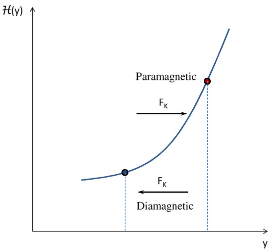
Due to the opposite microscopic responses, the paramagnetic fluids are attracted to and the diamagnetic fluids are repelled from regions of higher magnetic fields, which is illustrated in Figure 1.

In addition, the magnetic susceptibility of such fluids depends significantly on the local state, such as the density and temperature. In particular, paramagnetic fluids obey the Curie’s law, according to which $\chi =K\rho /T$, where K is a constant, while diamagnetic fluids satisfy $\chi ={\chi }_m\rho$, where ${\chi }_m$ is the mass susceptibility. Generally, the values of $\chi$ can vary widely depending on the fluid type and their phase, with the liquid state typically having about three-orders-of-magnitude-higher values of $\chi$ than their gaseous form. As such, if we consider the density dependence on temperature according to $\rho ={\rho }_{\mathrm{ref}}(1-{\alpha }_s)\theta$, where ${\alpha }_s$ is the thermal expansion coefficient, $\theta =T-T_{\mathrm{ref}}$, and the subscript ‘ref’ corresponds to a reference state, by applying a Taylor series to $\chi$, i.e., $\chi ={\chi }_{\mathrm{ref}}+{\left({\displaystyle \frac{\partial \chi }{\partial T}}\right)}_{\mathrm{ref}}\theta +{\left({\displaystyle \frac{\partial \chi }{\partial \rho }}\right)}_{\mathrm{ref}}(\rho -{\rho }_{\mathrm{ref}})$, we have the extended Bousinessq approximation [3] $\chi ={\chi }_{\mathrm{ref}}-{\chi }_{\mathrm{ref}}{\alpha }_s{\beta }_s\theta$, where ${\beta }_s=1+{\displaystyle \frac{1}{{\alpha }_s{T}_{\mathrm{ref}}}}$ and ${\beta }_s=1$ for paramagnetic and diamagnetic fluids, respectively. As a result, the Kelvin force ${\mathbf{f}}_K$ as expressed earlier can be interpreted as a buoyancy force, albeit in an artificial variable-gravity-like environment generated by the inhomogeneous magnetic fields. Such interesting characteristics can potentially be used to manipulate the flow and transport processes, especially in microgravity, where the Kelvin force can be particularly pronounced.

Interestingly, one of the earliest technical uses of the flow generated by the Kelvin force effects was by Pauling et al. [4], who developed a magnetic meter to measure the partial pressure of oxygen in gases. The study reported that the devised instrument might be used for paramagnetic and diamagnetic gases based on the magnetic susceptibility. Pioneering experimental work on the motion of fluids under the gradient magnetic fields was carried out by Wakayama [5], which led to several later investigations for different applications. He observed that oxygen or nitrogen mixed with oxygen was attracted by a magnetic field, and no magnetic field effect was detected for nitrogen or air. Butcher et al. [6] experimentally reported that the concentration gradient and the magnetic field gradient forces for paramagnetic species in solutions are equivalent for incompressible fluids, which are approximations of the Kelvin force and the Korteweg–Helmholtz force densities. Beaugnon and Tournier [7], in their seminal work, presented a successful experimental demonstration of the levitation of ordinary diamagnetic liquids, such as water, ethanol, and acetone, using the Kelvin force, which they also exploited to control natural convection in another study at about the same time [8]. Dibyendu et al. [9] used an analytical model for the motion of finite-sized diamagnetic particles of carboxylate microspheres in paramagnetic or diamagnetic fluid media. The results showed that structure formation of diamagnetic particles in diamagnetic fluid media is possible. Dodoo et al. [10] investigated the shaping and transport of diamagnetic drops using magnetostatic fields, and Feng et al. [11] experimentally and analytically introduced a portable and noncontact method for manipulating diamagnetic droplets on slippery liquid-infused porous surfaces using a single magnet. The results showed that the droplet volume, viscosity, vertical spacing on the critical migration velocity of water droplets, and diamagnetic nature of water played a role in the magnetic repulsive force. The physical basis of such levitation is designated as the magneto-Archimedes levitation, which was further demonstrated for a variety of fluids, including simple liquids such as water and organic materials, in more refined setups by other researchers [12,13,14].

Modulating, especially enhancing, the free convection process in electrically insulating fluids by means of inhomogeneous magnetic fields via the Kelvin buoyancy force has attracted considerable interest given its potential applications, and has resulted in some experimental, theoretical, and numerical investigations [3,7,15,16,17,18,19,20,21,22,23,24,25]. It may be noted that similar studies have been carried out for the case of artificial ferrofluids, starting from the work of Finlayson [26,27,28,29,30,31]. The use of the magnetic gradient force in other specialized applications, such as in the control of the combustion process and diffusion flames [32,33], water vaporization [34], the mixing process in aqueous solutions [12] and various others, were also successfully demonstrated. Early reviews on the Kelvin force effects are provided in [35,36]. It may be noted that Wakayama et al. [37] experimentally demonstrated an interesting and effective vertical acceleration control method that can vary continuously from normal gravity to close to zero gravity by exploiting the nature of the Kelvin force.

Recently, there has been considerable interest in the control of flow processes in crystals, especially involving protein crystals, using the Kelvin force [38], which has been reviewed by [39,40] and also in bio-physical flow contexts such as bacterial culture growth influenced by the buoyancy effects arising from nonuniform magnetic fields [41,42]. Furthermore, subsequently, Larachi et al. [43] experimentally studied the influence of inhomogeneous magnetic fields on the hydrodynamic properties of electrically insulating two-phase flows, such as gas–liquid systems. Kaneda et al. [44] conducted a numerical simulation of the spreading of a droplet on a surface, in which Marangoni convection is modulated through the Kelvin force, and Burgess and Premnath [45] developed an analytical solution for the fluid transport resulting from melting in the presence of such forces. Lei et al. [46] experimentally investigated the stability criterion of the magnetic separation of rare-earth ions, where mass transport causes instabilities in the enriched ions’ layer due to surface evaporation of the solution, which is levitated by the Kelvin force. In addition, they proposed a novel strategy for enhancing the magnetic field gradient for the room-temperature magnetic susceptibility and solutal expansion coefficient using partition assembly, which leads to improving the magnetic term of the Kelvin force [47]. Furthermore, Wang et al. [48] reported that non-uniform Kelvin forces are inclined to push diamagnetic fluids to regions with a lower magnetic field. Therefore, the Kelvin force improved the concentration polarization and current density in the channel for oxygen transfer within the air electrode of metal–air batteries by reducing the congestion of diamagnetic substances, such as $N_2$ and $H_2$O.

The main feature of intrinsic interest in fluid dynamics in such problems is the more detailed consideration of the generation mechanisms of the motions in electrically insulating fluids when subjected to magnetic and temperature gradients, in some cases. The latter results in spatial variations in the susceptibility in the Kelvin force via changes in the local density, as mentioned above, leading to a buoyant fluid motion. This fluid flow does not require gravity and is sometimes termed the “magnetothermal wind” or “magnetothermal convection” [49,50]. Although much of the work in this area is experimental or numerical in some cases, analytical studies that can provide fundamental insights into such problems are, by and large, lacking [51,52].

A related prototypical fluid dynamics problem, which is the subject of this paper, is the generation of an intruding viscous fluid motion of an electrically insulating fluid into an ambient fluid on a rigid surface caused by a horizontal Kelvin buoyancy force. The latter arises when there is contrast in the susceptibilities of the intruding and ambient fluids, which may be caused by density and/or temperature changes, as discussed earlier, in the presence of a specific inhomogeneous spatial distribution of the magnetic field. For example, under microgravity conditions, one may induce and appropriately control the spreading of common fluids such as blobs of water or oil or even molten glass, all of which are diamagnetic, solely in the presence of the Kelvin force. Such a viscous current caused by the Kelvin force with susceptibility contrasts has a particularly close analogy with the classical viscous gravity current, which was first studied theoretically and experimentally in the pioneering work of Huppert [53] (see also [54,55,56] for recent reviews on this subject). In particular, both require differences in certain fluid properties, such as the magnetic susceptibility or density, between the intruding and ambient fluids to create a horizontal buoyancy, with the former driven by an artificially controllable gravity-like body force (Kelvin force), while the latter is driven by a constant body force (gravity).

In this paper, we developed a new mathematical model for planar, i.e., two-dimensional, and axisymmetric viscous currents generated by a horizontal buoyancy due to the Kelvin force, i.e., in the presence of magnetic field gradients when there is a difference between the magnetic susceptibilities of the intruding and ambient fluids. The source of the susceptibility difference could be differences in the temperature, density, or both of intruding and ambient electrically insulating fluids, though our focus is on isothermal solutions. As such, in the absence of gravity, the Kelvin force can provide a driving mechanism for spreading common fluids, which can also be exploited in other situations. For example, by manipulating the spatial variation in magnetic fields, the spreading extent and shape of various currents can be controlled in potential technological applications in microgravity or specific earth-bound applications (e.g., viscous currents in protein crystal growth problems or material-processing applications). The model is developed based on considerations of slow viscous flow, i.e., under the standard lubrication approximation, analogous to the classical viscous gravity current [53]. Following that study, we also neglected the effect of capillary force, assuming that the magnetic Bond number, $B{o}_m$ is much larger than 1. This leads to self-similar solutions for the shape of the viscous current and for spreading relationships, based on scaling considerations, when a power law prescribes the spatial variation in the magnetic field. For a prescribed form of the source flux of the intruding fluids, it will be shown that a family of scaling laws exists for the spreading rate and the film thickness of the viscous current, which is found to depend on the sharpness of the magnetic field gradient, characterized as the exponent of a power law. The following section presents a derivation of this new model, followed by a discussion of the resulting key findings.

2. Mathematical Model

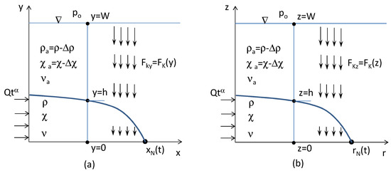
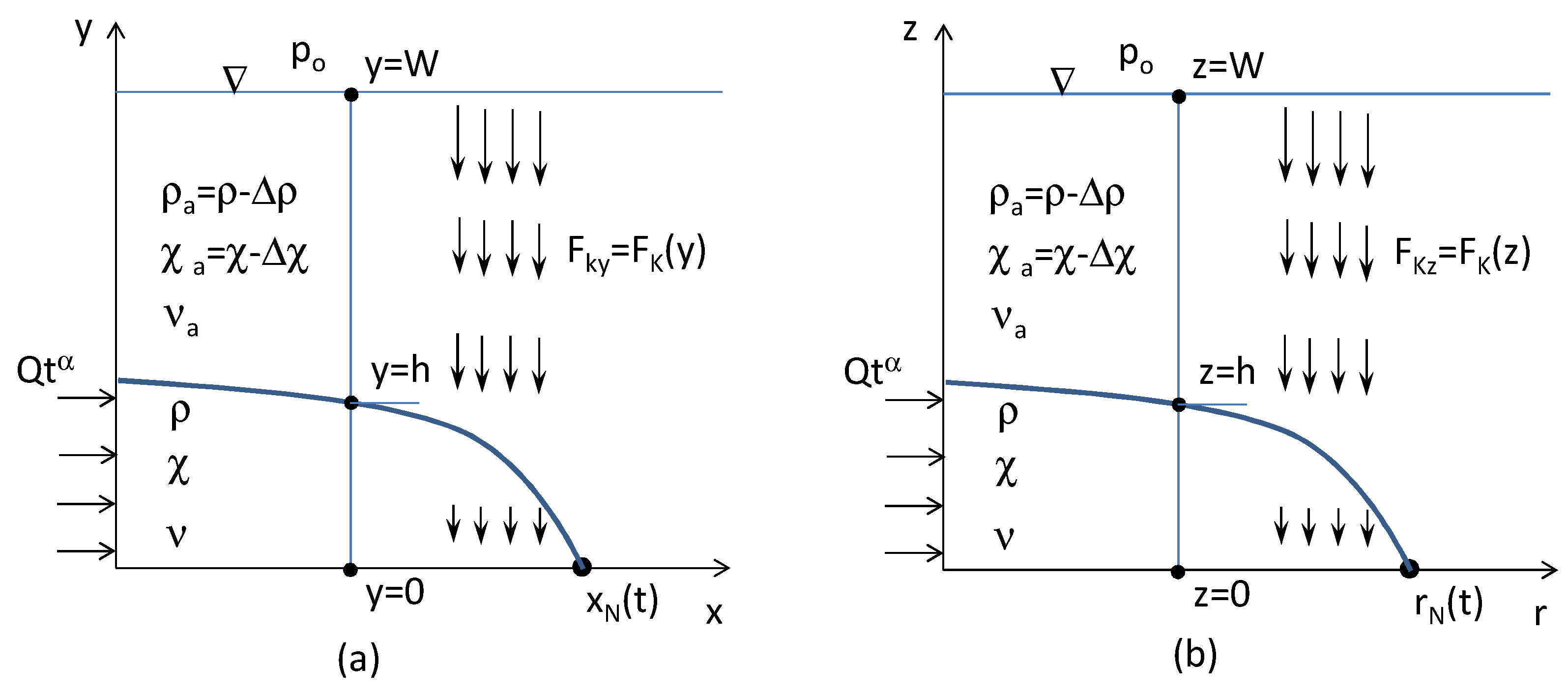
A schematic of the physical configuration representing the horizontal viscous current of an electrically insulating fluid into an ambient fluid (whose properties are designated with subscript ‘a’) in the presence of an inhomogeneous magnetic field in the normal direction in the two-dimensional and axisymmetric coordinate systems is shown in Figure 2.

While, for the generality of the derivation, we consider a time-dependent influx $Q{t}^{\alpha }$, our main interest lies in the crucial special case involving the constant inflow condition ($\alpha =0$), which we use to gain physical insights. Due to a balance between the buoyancy (Kelvin) and viscous forces, a viscous current propagates on a rigid horizontal surface, which depends on the density $\rho$, magnetic susceptibility $\chi$ and kinematic viscosity $\nu$ of the fluids. The locations of the current nose in the two-dimensional and axisymmetric coordinate systems are denoted as $x_N\left(t\right)$ and $r_N\left(t\right)$, respectively. The shape and rate of propagation of such a low-Reynolds-number current propagating over a rigid surface can be determined by applying the lubrication approximation [57,58]. While gravity is considered along with the Kelvin force at the beginning of our formulation, since our chief interest is in generating flow solely due to the latter, the former is dropped while determining the analytical solution. Nevertheless, the discussion section illustrates their coupled role in a special case.

2.1. Two-Dimensional Viscous Current

The equations of the parallel viscous flow of density $\rho$ and kinematic viscosity $\nu$ in the main and normal directions may, respectively, be written as

$$\begin{array}{ccc}\hfill \rho {\displaystyle \frac{\partial u}{\partial t}}& =& \rho \nu {\displaystyle \frac{{\partial }^{2}u}{\partial y^2}}-{\displaystyle \frac{\partial p}{\partial x}},\hfill \end{array}$$

(1)

$$\begin{array}{ccc}\hfill \hspace{1em}\hspace{1em}0& =& -{\displaystyle \frac{\partial p}{\partial y}}-\rho g+F_{Ky},\hfill \end{array}$$

(2)

where u and p are the fluid velocity and pressure, respectively, and $F_{Ky}$ is the Kelvin force, which depends on the spatial variation in the magnetic field $\mathcal{H}\left(y\right)$ in the normal direction and is given by [3,45]

$$F_{K\left(y\right)}={\mu }_o{\displaystyle \frac{\chi }{2}}{\displaystyle \frac{\partial {\mathcal{H}}^2\left(y\right)}{\partial y}}.$$

(3)

By integrating Equation (2) across the viscous current, we have

$${\int }_y^{W}dp=-{\int }_y^h\rho gdy-{\int }_h^W\rho gdy+{\mu }_o{\int }_y^h{\displaystyle \frac{\chi }{2}}{\displaystyle \frac{\partial }{\partial y}}\mathcal{H}{\left(y\right)}^{2}dy+{\mu }_o{\int }_h^W{\displaystyle \frac{\chi }{2}}{\displaystyle \frac{\partial }{\partial y}}\mathcal{H}{\left(y\right)}^{2}dy.$$

Then, using the pressure boundary conditions at $y=W$ as $p=p_o$, the pressure field variation across the current becomes

$$p\left(y\right)=p_o+\rho g(h-y)+{\rho }_{a}g(W-h)-{\displaystyle \frac{{\mu }_o}{2}}\chi \left[{\mathcal{H}}^2\left(h\right)-{\mathcal{H}}^2\left(y\right)\right]-{\displaystyle \frac{{\mu }_o}{2}}{\chi }_a\left[{\mathcal{H}}^2\left(W\right)-{\mathcal{H}}^2\left(h\right)\right],$$

(4)

where W and h are the characteristic length scales of the ambient and intruding fluids, respectively. This provides the expression for the pressure gradient in the x-direction as ${\displaystyle \frac{\partial p}{\partial x}}=\rho g{\displaystyle \frac{\partial h}{\partial x}}-{\rho }_{a}g{\displaystyle \frac{\partial h}{\partial x}}-{\displaystyle \frac{{\mu }_o}{2}}\chi {\displaystyle \frac{\partial }{\partial x}}{\mathcal{H}}^2\left(h\right)+{\displaystyle \frac{{\mu }_o}{2}}{\chi }_a{\displaystyle \frac{\partial }{\partial x}}{\mathcal{H}}^2\left(h\right)$. By rewriting the density and the susceptibility of the intruding fluid as $\rho ={\rho }_a+\mathsf{\Delta }\rho$ and $\chi ={\chi }_a+\mathsf{\Delta }\chi$, we get

$${\displaystyle \frac{\partial p}{\partial x}}=\mathsf{\Delta }\rho g{\displaystyle \frac{\partial h}{\partial x}}-{\displaystyle \frac{{\mu }_o}{2}}\mathsf{\Delta }\chi {\displaystyle \frac{\partial }{\partial x}}{\mathcal{H}}^2\left(h\right),$$

(5)

where $\mathsf{\Delta }\rho$ and $\mathsf{\Delta }\chi$ are the differences in the density and magnetic susceptibility between the intruding and ambient fluids, respectively. It is assumed that the effectively isothermal/constant property variations remain constant when subjected to externally imposed contrasts. To perform an order-of-magnitude analysis, we define the characteristic length scales along the main flow and lateral directions as L and H, respectively, and the characteristic velocity and time scales as U and $T=L/U$, respectively. Thus, for Equation (1), we estimate the ratio of the inertial and viscous forces as $\rho U/T:\mu U/H^2$, where $\mu$ is the dynamic shear viscosity. It is assumed that the Reynold number, ($UH/\nu$), and the aspect ratio, ($H/\mathrm{Ł}$), are much less than 1, i.e., under the lubrication approximation, the film is taken to be thin, and the flow to be creeping. This implies that inertia can be neglected if $U{H}^2/\nu L\ll 1$, which is readily satisfied for slow viscous flow in thin films. Thus, this lubrication approximation reduces the equation of motion to $\nu {\displaystyle \frac{{\partial }^{2}u}{\partial y^2}}={\displaystyle \frac{1}{\rho }}{\displaystyle \frac{\partial p}{\partial x}}$, which, upon substituting Equation (5), becomes

$$\nu {\displaystyle \frac{{\partial }^{2}u}{\partial y^2}}=g^{\prime }{\displaystyle \frac{\partial h}{\partial x}}+\tilde{K}{\displaystyle \frac{\partial }{\partial x}}{\mathcal{H}}^2\left(h\right),$$

(6)

where $g^{\prime }={\displaystyle \frac{\mathsf{\Delta }\rho }{\rho }}g$ and $\tilde{K}=-{\displaystyle \frac{{\mu }_o}{2}}{\displaystyle \frac{\mathsf{\Delta }\chi }{\rho }}$.

For ease of analysis, we prescribe the following power law variation for the square of the magnetic field

$${\mathcal{H}}^2\left(y\right)={\mathcal{H}}_o^2+{\mathcal{H}}_o^2{ϵ}^2{y}^{2m},$$

(7)

where ${\mathcal{H}}_o$ is a constant field outside of fluids, $ϵ$ is a parameter that controls the magnitude of field variation within the fluid, and m is the power law exponent that characterizes the steepness of the field variation spatially. As such, the above equation can be considered as an idealization or approximate representation of the magnetic field that captures different gradient regimes by adjusting the exponent m and enables an analytical characterization of the fluid dynamic phenomena involved. Hence, from Equation (6), we get ${\displaystyle \frac{\partial }{\partial x}}{\mathcal{H}}^2\left(h\right)=2m{\mathcal{H}}_o^2{ϵ}^2{h}^{2m-1}{\displaystyle \frac{\partial h}{\partial x}}$. Thus, Equation (6) becomes

$$\nu {\displaystyle \frac{{\partial }^{2}u}{\partial y^2}}=g^{\prime }{\displaystyle \frac{\partial h}{\partial x}}+K^{\prime }{h}^{2m-1}{\displaystyle \frac{\partial h}{\partial x}},$$

(8)

where

$$K^{\prime }=-2m{\displaystyle \frac{{\mu }_0}{2}}{\displaystyle \frac{\mathsf{\Delta }\chi }{\rho }}{ϵ}^2{\mathcal{H}}_o^2,$$

(9)

which we shall the Kelvin force parameter. Note that, when $m=0$, the above reduces to the classical formulation [53]. To complete our formulation, we augment Equation (9) by imposing the no-slip and free surface boundary conditions $u(y=0)=0$ and $\nu {\displaystyle \frac{\partial u}{\partial y}}(y=h)=0$, respectively, as well as the following global continuity equation [53]:

$${\int }_0^{x_N\left(t\right)}h(x,t)dy=Q{t}^{\alpha }.$$

(10)

We now try to isolate the case involving a purely Kelvin force-driven viscous current so that its influence can be clearly elucidated. Thus, the terrestrial gravity is assumed to be negligible so that this situation could correspond to the free space or a suitable microgravity condition, i.e., $g^{\prime }=0$. Interestingly, this also allows for the development of a similarity solution from a mathematical point of view, as we shall see in what follows. The latter aspect is useful for making certain concrete theoretical deductions, such as scaling laws. By integrating Equation (8) with $g^{\prime }=0$ with the above boundary conditions, we readily obtain the following parabolic velocity profile:

$$u\left(y\right)=-{\displaystyle \frac{K^{\prime }{h}^{2m-1}}{2\nu }}{\displaystyle \frac{\partial h}{\partial x}}y(2h-y),$$

(11)

which then yields the flux q as $q={\int }_0^{h}udy=-{\displaystyle \frac{K^{\prime }{h}^{2m+2}}{3\nu }}{\displaystyle \frac{\partial h}{\partial x}}$. By using this and applying the local mass conservation, i.e., ${\displaystyle \frac{\partial h}{\partial t}}+{\displaystyle \frac{\partial q}{\partial x}}=0$, we get the following evolution equation for the local thickness of the viscous current:

$${\displaystyle \frac{\partial h}{\partial t}}={\displaystyle \frac{\partial }{\partial x}}\left[{\displaystyle \frac{K^{\prime }}{3\nu }}{h}^{2m+2}{\displaystyle \frac{\partial h}{\partial x}}\right].$$

(12)

2.1.1. Scaling Analysis

Before a more formal mathematical analysis is considered, we performed the following scaling analysis based on the orders-of-magnitude estimates [59], which provided the scaling relationships among different quantities. As such, this straightforward approach is physically appealing and generally leads to the same overall outcomes involving scaling laws by means of a more involved mathematical procedure. Momentum balance with $g^{\prime }=0$ gives (see Equation (8))

$$\nu {\displaystyle \frac{U}{H^2}}\sim K^{\prime }{\displaystyle \frac{H^{2m}}{L}},$$

(13)

while the global continuity equation (see Equation (10)) yields

$$HL\sim Q{T}^{\alpha }.$$

(14)

Now, using the characteristic velocity scale $U\sim L/T$ in Equation (13) and eliminating H using Equation (14), we have the following scaling relationship for the spreading distance:

$$L\sim {\left[{\displaystyle \frac{K^{\prime }}{\nu }}{Q}^{2m+2}{T}^{\alpha (2m+2)+1}\right]}^{{\displaystyle \frac{1}{2m+4}}}.$$

(15)

Since no further constraints apply to these scales, there is no other choice but to simply apply time scaling by means of the elapsed time t, i.e., $T\sim t$. Hence, we can deduce the following relationship for the extent of the nose of the current:

$$x_N={\eta }_N{\left[{\displaystyle \frac{K^{\prime }}{\nu }}{Q}^{2m+2}{t}^{\alpha (2m+2)+1}\right]}^{{\displaystyle \frac{1}{2m+4}}},$$

(16)

where ${\eta }_N$ is a proportionality constant to be determined. By using the expression for the Kelvin force parameter $K^{\prime }$ (see Equation (9)), it is clear that $x_N$ for the two-dimensional current varies according to the fluid properties and the imposed field as ${\left[-2m{\displaystyle \frac{{\mu }_0}{2\nu }}{\displaystyle \frac{\mathsf{\Delta }\chi }{\rho }}{ϵ}^2{\mathcal{H}}_o^2\right]}^{{\displaystyle \frac{1}{2m+4}}}$. Furthermore, $x_N$ depends on time as $t^{{\displaystyle \frac{\left(\right(2m+2)\alpha +1)}{(2m+4)}}}$. From Equations (14) and (15), we obtain the following scaling law for the characteristic scale of the film thickness of the viscous current:

$$H\sim {\left[{\displaystyle \frac{\nu }{K^{\prime }}}{\displaystyle \frac{Q^2}{t^{1-2\alpha }}}\right]}^{{\displaystyle \frac{1}{(2m+4)}}}.$$

(17)

It follows that H depends on magnetic properties as ${\left[-2m{\displaystyle \frac{{\mu }_0}{2}}{\displaystyle \frac{\mathsf{\Delta }\chi }{\rho }}{ϵ}^2{\mathcal{H}}_o^2\right]}^{-{\displaystyle \frac{1}{2m+4}}}$.

2.1.2. Similarity Solution for the Structure of the Kelvin-Force-Generated 2D Viscous Current

Based on the above scaling analysis, we can then define the following similarity variable $\eta$ for the independent variable and $f\left(\eta \right)$ for the film thickness h, respectively:

$$\begin{array}{ccc}\hfill \hspace{1em}\eta & =& x/L={\left[{\displaystyle \frac{K^{\prime }}{\nu }}{Q}^{2m+2}{t}^{\alpha (2m+2)+1}\right]}^{-{\displaystyle \frac{1}{2m+4}}}x,\hfill \end{array}$$

(18)

$$\begin{array}{ccc}\hfill h& =& Hf\left(\eta \right)={\left[{\displaystyle \frac{\nu }{K^{\prime }}}{\displaystyle \frac{Q^2}{t^{1-2\alpha }}}\right]}^{{\displaystyle \frac{1}{(2m+4)}}}f\left(\eta \right).\hfill \end{array}$$

(19)

where $f\left(\eta \right)$ is the similarity function that determines the shape of the viscous film, which is yet to be determined. By substituting Equations (18) and (19) in the evolution equation for the film thickness, i.e., Equation (12), and after some simplification and rearrangement, we get the following self-similar non-linear ordinary differential equation for the scaled thickness $f\left(\eta \right)$ of the viscous current:

$$-{\displaystyle \frac{\left(\right(2m+2)\alpha +1)}{(2m+4)}}\eta {\displaystyle \frac{df}{d\eta }}-{\displaystyle \frac{(1-2\alpha )}{(2m+4)}}f={\displaystyle \frac{1}{3}}{\displaystyle \frac{d}{d\eta }}\left(f^{(2m+2)}{\displaystyle \frac{df}{d\eta }}\right).$$

(20)

This is supplemented by the global continuity equation (Equation (10)), written in terms of similarity variables (Equations (18) and (19)), as

$${\int }_0^{{\eta }_N}f\left(\eta \right)d\eta =1,$$

(21)

as well as the additional boundary condition at the nose of the current as $f(\eta ={\eta }_N)=0$.

For the purpose of gaining insight, we considered the important special case with $\alpha =0$ in this work, which also immediately admits a closed-form analytical solution. Indeed, with $\alpha =0$ in Equation (20), we get $-{\displaystyle \frac{1}{(2m+4)}}{\displaystyle \frac{d}{d\eta }}\left(f\eta \right)={\displaystyle \frac{1}{3}}{\displaystyle \frac{d}{d\eta }}\left(f^{(2m+2)}{\displaystyle \frac{df}{d\eta }}\right)$, which has the form of a non-linear diffusion-type equation and can be integrated to yield

$$f\left(\eta \right)={\left[{\displaystyle \frac{3}{2}}{\displaystyle \frac{(m+1)}{(m+2)}}\right]}^{{\displaystyle \frac{1}{(2m+2)}}}{\left({\eta }_N^2-{\eta }^2\right)}^{{\displaystyle \frac{1}{(2m+2)}}},$$

(22)

where ${\eta }_N$ is the scaled extent of the nose of the viscous current, whose explicit expression can be obtained from the global conservation condition. Indeed, by substituting Equation (22) into Equation (21) and after some simplifications and rearrangement, we get

$${\eta }_N={\left({\displaystyle \frac{2}{3C_m}}\right)}^{{\displaystyle \frac{1}{(2m+4)}}}{\left[{\displaystyle \frac{\sqrt{\pi }}{2(m+2)}}{\displaystyle \frac{\mathsf{\Gamma }\left(\frac{1}{2m+2}\right)}{\mathsf{\Gamma }\left(\frac{m+2}{2m+2}\right)}}\right]}^{-C_m},$$

(23)

where $C_m={\displaystyle \frac{(m+1)}{(m+2)}}$ and $\mathsf{\Gamma }\left(s\right)$ is the standard gamma function with argument s. Thus, Equations (22) and (23) provide the structure of the planar viscous current generated by the Kelvin force. Moreover, the local shear stress on the rigid surface can be estimated from the Newton’s law of viscosity and using the velocity profile given in Equation (11). A detailed analysis in this regard is included in Appendix A.1.

2.2. Axisymmetric Viscous Current

The derivation of the axisymmetric viscous flow in the presence of the Kelvin force under the lubrication approximation is analogous to the two-dimensional case. The simplified governing equations in the radial and axial directions become

$$\begin{array}{ccc}\hfill \rho {\displaystyle \frac{\partial u}{\partial t}}& =& \rho \nu {\displaystyle \frac{{\partial }^{2}u}{\partial z^2}}-{\displaystyle \frac{\partial p}{\partial r}},\hfill \end{array}$$

(24)

$$\begin{array}{ccc}\hfill \hspace{1em}\hspace{1em}0& =& -{\displaystyle \frac{\partial p}{\partial z}}-\rho g+F_{Kz},\hfill \end{array}$$

(25)

where the axial Kelvin force $F_{Kz}$ can be represented as $F_{Kz}={\mu }_o{\displaystyle \frac{\chi }{2}}{\displaystyle \frac{\partial {\mathcal{H}}^2\left(z\right)}{\partial z}}$. The integration of Equation (25) provides an expression for the pressure field, which is similar to Equation (4), with the replacement of y by z. Thus, the radial pressure gradient can be written as

$${\displaystyle \frac{\partial p}{\partial r}}=\mathsf{\Delta }\rho g{\displaystyle \frac{\partial h}{\partial r}}-{\displaystyle \frac{{\mu }_o}{2}}\mathsf{\Delta }\chi {\displaystyle \frac{\partial }{\partial r}}{\mathcal{H}}^2\left(h\right).$$

(26)

As in the two-dimensional case, the above can be further simplified by means of the order-of-magnitude scaling arguments. Considering R and H to be the characteristic length scales in the radial and lateral directions, respectively, and U and $T=R/U$ to be the velocity and time scales, respectively, the inertial force in Equation (24) can be neglected if $U{H}^2/\nu R\ll 1$. As a result, Equation (24) reduces further, which can be rearranged as

$$\nu {\displaystyle \frac{{\partial }^{2}u}{\partial z^2}}=g^{\prime }{\displaystyle \frac{\partial h}{\partial r}}+\tilde{K}{\displaystyle \frac{\partial }{\partial r}}{\mathcal{H}}^2\left(h\right),$$

(27)

where the expressions for $g^{\prime }$ and $\tilde{K}$ are the same as in the two-dimensional case. As before, we specify the following power law variation for the square of the magnetic field:

$${\mathcal{H}}^2\left(z\right)={\mathcal{H}}_o^2+{\mathcal{H}}_o^2{ϵ}^2{z}^{2m}.$$

(28)

As a result, Equation (27) simplifies further to the following:

$$\nu {\displaystyle \frac{{\partial }^{2}u}{\partial z^2}}=g^{\prime }{\displaystyle \frac{\partial h}{\partial r}}+K^{\prime }{h}^{2m-1}{\displaystyle \frac{\partial h}{\partial r}},$$

(29)

where $K^{\prime }$ is the Kelvin force parameter defined as before. This equation is supplemented by the boundary conditions $u(z=0)=0$ and $\nu {\displaystyle \frac{\partial u}{\partial z}}(z=h)=0$ and the following global conservation equation:

$${\int }_0^{r_N\left(t\right)}2\pi rh(x,t)dr=Q{t}^{\alpha }.$$

(30)

By again isolating the pure Kelvin force effects by setting $g^{\prime }=0$, and integrating Equation (29) with the boundary conditions given above, we obtain the velocity profile across a section of the viscous current as $u\left(z\right)=-{\displaystyle \frac{K^{\prime }{h}^{2m-1}}{2\nu }}{\displaystyle \frac{\partial h}{\partial r}}z(2h-z)$. Thus, the flux is $q={\int }_0^{h}udz=-{\displaystyle \frac{K^{\prime }{h}^{2m+2}}{3\nu }}{\displaystyle \frac{\partial h}{\partial r}}$, from which the local conservation of mass ${\displaystyle \frac{\partial h}{\partial t}}+{\displaystyle \frac{1}{r}}{\displaystyle \frac{\partial }{\partial r}}\left(rq\right)=0$ reduces to the following equation for the evolution of the thickness of the axisymmetric viscous current:

$${\displaystyle \frac{\partial h}{\partial t}}={\displaystyle \frac{1}{r}}{\displaystyle \frac{\partial }{\partial r}}\left[r{\displaystyle \frac{K^{\prime }}{3\nu }}{h}^{2m+2}{\displaystyle \frac{\partial h}{\partial r}}\right].$$

(31)

2.2.1. Scaling Analysis

We performed a scaling analysis on the above formulation to provide some physical insights, just as in the two-dimensional case. Equation (29) with $g^{\prime }=0$ reads

$$\nu {\displaystyle \frac{U}{H^2}}\sim K^{\prime }{\displaystyle \frac{H^{2m}}{R}},$$

(32)

while the global conservation implies

$$H{R}^2\sim Q{T}^{\alpha }.$$

(33)

By substituting the velocity scale $U\sim R/T$ into Equation (32), the scaling law for the spreading distance R can be obtained after eliminating H using Equation (33). Thus, we have

$$R\sim {\left[{\displaystyle \frac{K^{\prime }}{\nu }}{Q}^{2m+2}{T}^{\alpha (2m+2)+1}\right]}^{{\displaystyle \frac{1}{4m+6}}}.$$

(34)

We take $T\sim t$ since no further constraints exist on the scalings. As a result, we can write the expression for the location of the nose $r_N$ in terms of the elapsed time t as

$$r_N={\xi }_N{\left[{\displaystyle \frac{K^{\prime }}{\nu }}{Q}^{2m+2}{t}^{\alpha (2m+2)+1}\right]}^{{\displaystyle \frac{1}{4m+6}}},$$

(35)

where ${\xi }_N$ is a proportionality constant to be determined. Clearly, $r_N$ for axisymmetric viscous flow depends on the fluid properties and the imposed field as ${\left[-2m{\displaystyle \frac{{\mu }_0}{2\nu }}{\displaystyle \frac{\mathsf{\Delta }\chi }{\rho }}{ϵ}^2{\mathcal{H}}_o^2\right]}^{{\displaystyle \frac{1}{4m+6}}}$ and on the elapsed time as $t^{{\displaystyle \frac{\left(\right(2m+2)\alpha +1)}{(4m+6)}}}$. Finally, the scaling relationship for the thickness of the viscous current can be obtained from Equations (33) and (34) as

$$H\sim {\left[{\displaystyle \frac{\nu }{K^{\prime }}}{\displaystyle \frac{Q}{t^{1-\alpha }}}\right]}^{{\displaystyle \frac{1}{(2m+3)}}}.$$

(36)

It can be seen that the film thickness is dependent on the magnetic properties as ${\left[-2m{\displaystyle \frac{{\mu }_0}{2}}{\displaystyle \frac{\mathsf{\Delta }\chi }{\rho }}{ϵ}^2{\mathcal{H}}_o^2\right]}^{-{\displaystyle \frac{1}{2m+3}}}$.

2.2.2. Similarity Solution for the Structure of the Kelvin-Force-Generated Axisymmetric Viscous Current

We can now obtain a similarity solution by exploiting the above scaling considerations. In particular, we now define the similarity variable $\xi$ for the independent variables and film thickness h, respectively, as

$$\begin{array}{ccc}\hfill \hspace{1em}\xi & =& r/R={\left[{\displaystyle \frac{K^{\prime }}{\nu }}{Q}^{2m+2}{t}^{\alpha (2m+2)+1}\right]}^{-{\displaystyle \frac{1}{4m+6}}}r,\hfill \end{array}$$

(37)

$$\begin{array}{ccc}\hfill h& =& H\varphi \left(\xi \right)={\left[{\displaystyle \frac{\nu }{K^{\prime }}}{\displaystyle \frac{Q}{t^{1-\alpha }}}\right]}^{{\displaystyle \frac{1}{(2m+3)}}}\varphi \left(\xi \right).\hfill \end{array}$$

(38)

where $\varphi \left(\xi \right)$ is the similarity function that determines the structure of the viscous film. When Equations (37) and (38) are substituted into Equation (31), we can obtain the self-similar ordinary differential equation for $\varphi \left(\xi \right)$. The details of the various steps involved in this derivation are given in Appendix A.1 for convenience, which, after certain simplifications, reads as

$$-{\displaystyle \frac{\left(\right(2m+2)\alpha +1)}{(4m+6)}}{\xi }^2{\displaystyle \frac{d\varphi }{d\xi }}-{\displaystyle \frac{2(1-\alpha )}{(4m+6)}}\xi \varphi ={\displaystyle \frac{1}{3}}{\displaystyle \frac{d}{d\xi }}\left(\xi {\varphi }^{(2m+2)}{\displaystyle \frac{d\varphi }{d\xi }}\right).$$

(39)

This is augmented by the boundary condition at the nose of the current as $\varphi (\xi ={\xi }_N)=0$ and the global continuity constraint, i.e., Equation (30), which can be rewritten in terms of the above similarity variables as

$${\int }_0^{{\xi }_N}2\pi \xi \varphi \left(\xi \right)d\xi =1.$$

(40)

As in the two-dimensional case, we consider the special case with $\alpha =0$, which yields an explicit analytical solution, as we shall see next. For this case, Equation (39) reduces to $-{\displaystyle \frac{1}{(4m+6)}}{\xi }^2{\displaystyle \frac{d\varphi }{d\xi }}-{\displaystyle \frac{2}{(4m+6)}}\left(\xi \varphi \right)={\displaystyle \frac{1}{3}}{\displaystyle \frac{d}{d\xi }}\left({\xi }^{(2m+2)}{\displaystyle \frac{d\varphi }{d\xi }}\right)$, which can be immediately integrated. We get

$$\varphi \left(\xi \right)={\left[{\displaystyle \frac{3}{4}}{\displaystyle \frac{(2m+2)}{(2m+3)}}\right]}^{{\displaystyle \frac{1}{(2m+2)}}}{\left({\xi }_N^2-{\xi }^2\right)}^{{\displaystyle \frac{1}{(2m+2)}}},$$

(41)

where ${\xi }_N$ is the scaled extent of the nose of the axisymmetric viscous current. The latter quantity can be deduced from the global conservation constraint. Thus, by using Equation (41) in Equation (40) and after some simplification, we obtain ${\xi }_N$ as

$${\xi }_N={\left[{\left({\displaystyle \frac{E_m}{m+1}}\right)}^{E_m}{\displaystyle \frac{1}{3\times 2^{E_m-2}\times {\pi }^{E_m-1}}}\right]}^{{\displaystyle \frac{1}{2E_m}}},$$

(42)

where $E_m=2m+3$. The above two equations determine the shape of the axisymmetric viscous current induced by the Kelvin force for a given m. In the next section, we discuss some key findings from newly developed physical models for the structures of the 2D and axisymmetric Kelvin-force-generated viscous currents.

3. Results and Discussion

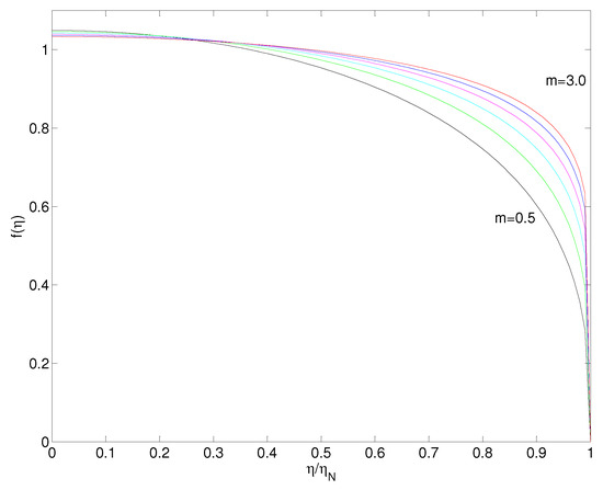
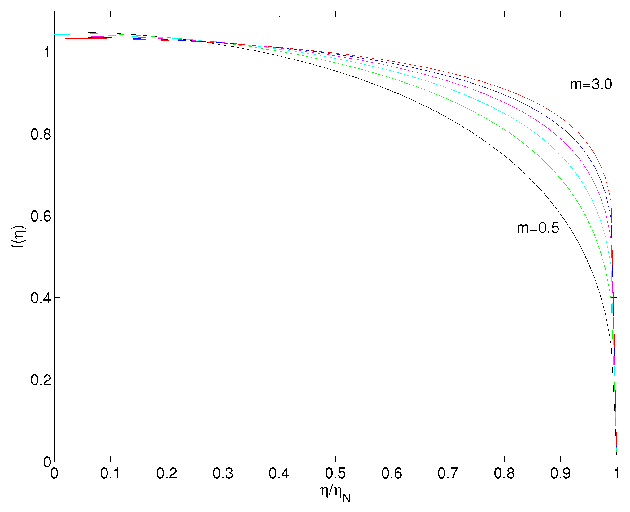
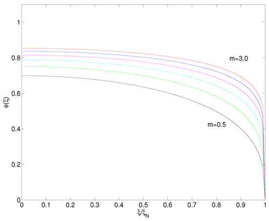
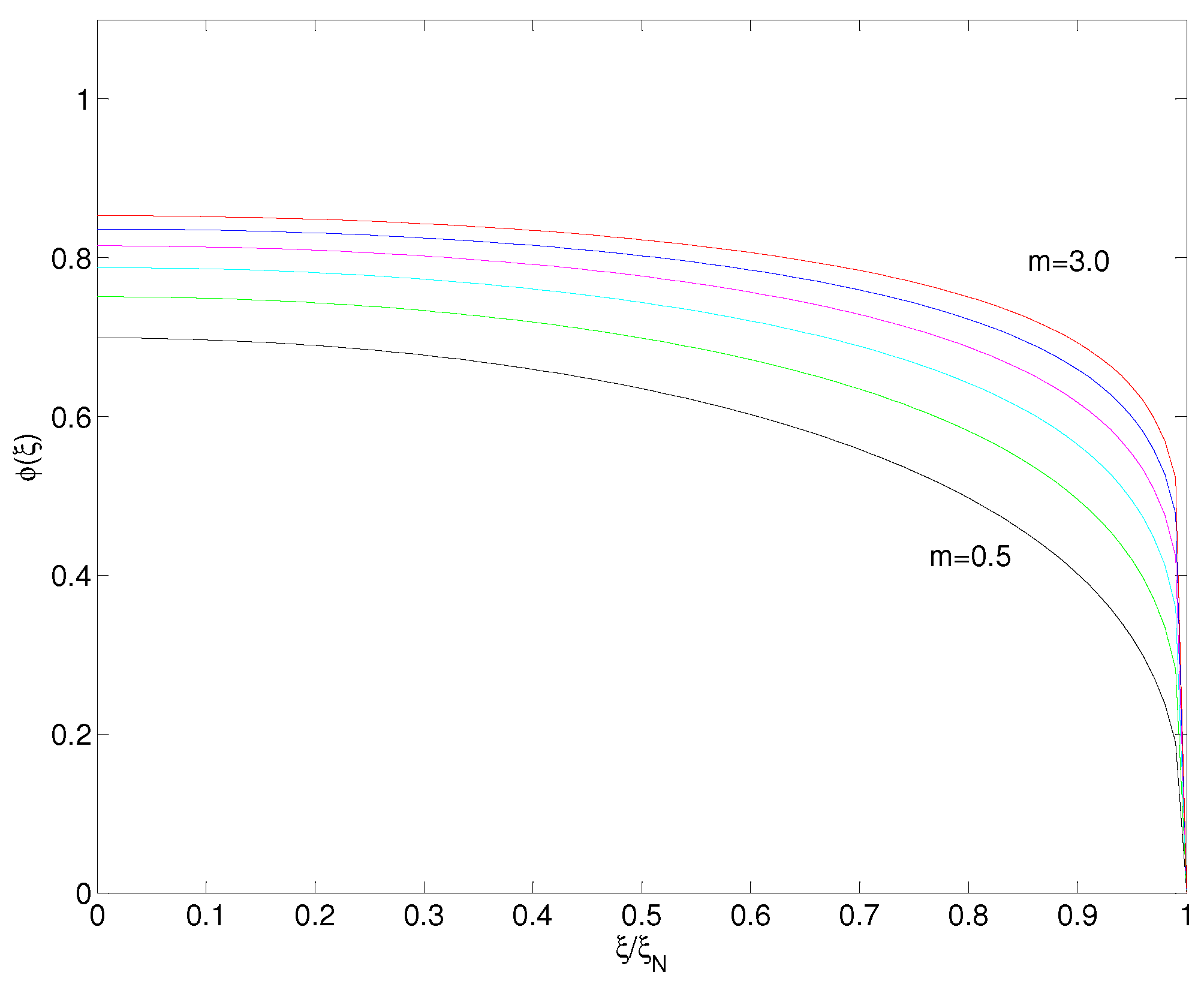
Figure 3 shows the shape of the two-dimensional viscous current obtained by plotting Equation (22) with the use of Equation (23). Similarly, the structure of the axisymmetric viscous current generated by the Kelvin force (using Equation (41) with (42)) is presented in Figure 4. Essentially, contrasts in the magnetic susceptibilities of the intruding and ambient fluids, which can be caused externally due to differences in their densities or temperatures, set up the viscous flow when subjected to a nonuniform background magnetic field. As such, this unique viscous current phenomenon can occur even in the absence of terrestrial gravity, as the model elucidates. In general, as the exponent for the spatial variation in the magnetic field strength m increases, it is seen that the shape of the current in the vicinity of its nose becomes progressively more blunt. This is a manifestation of the greater magnitude of the Kelvin buoyancy force with the normal coordinates as the spatial gradient of the field (or m) increases, thereby pushing the free surface of the intruding fluid further into the bulk region of the ambient fluid, as the rigid surface counteracts the bottom of the nose through viscous forces (see Appendix A.1 for further details).

The scaling relationships for the spreading distance and the film thickness in terms of different governing parameters as a function of the exponent m for the two-dimensional and the axisymmetric viscous currents are presented in

Table 1. Scaling relationships involving different characteristic parameters as a function of m for the two-dimensional viscous current with $\alpha =0$ induced by the Kelvin force. Here, $x_N\sim t^p$, $h\sim t^{-q}$, $x_N\sim {\left(ϵ{\mathcal{H}}_0\right)}^l$, $h\sim {\left(ϵ{\mathcal{H}}_0\right)}^{-n}$, $x_N\sim Q^a$, $h\sim Q^b$, $x_N\sim {(\mathsf{\Delta }\chi /\rho \nu )}^x$ and $h\sim {(\mathsf{\Delta }\chi /\rho \nu )}^{-y}$.

m	${\mathit{\eta }}_{\mathit{N}}$	p	q	l	n	a	b	x	y
0	$1.2125$	$1/4$	$1/4$	$1/2$	$1/2$	$1/2$	$1/2$	$1/4$	$1/4$
$1/2$	$1.1329$	$1/5$	$1/5$	$2/5$	$2/5$	$3/5$	$2/5$	$1/5$	$1/5$
1	$1.0939$	$1/6$	$1/6$	$1/3$	$1/3$	$2/3$	$1/3$	$1/6$	$1/6$
$3/2$	$1.0714$	$1/7$	$1/7$	$2/7$	$2/7$	$5/7$	$2/7$	$1/7$	$1/7$
2	$1.0570$	$1/8$	$1/8$	$1/4$	$1/8$	$3/4$	$1/4$	$1/8$	$1/8$
$5/2$	$1.0470$	$1/9$	$1/9$	$2/9$	$2/9$	$7/9$	$2/9$	$1/9$	$1/9$
3	$1.0398$	$1/10$	$1/10$	$1/5$	$1/5$	$4/5$	$1/5$	$1/10$	$1/10$

and

Table 2. Scaling relationships involving different characteristic parameters as a function of m for the axisymmetric viscous current with $\alpha =0$ induced by the Kelvin force. Here, $r_N\sim t^p$, $h\sim t^{-q}$, $r_N\sim {\left(ϵ{\mathcal{H}}_0\right)}^l$, $h\sim {\left(ϵ{\mathcal{H}}_0\right)}^{-n}$, $r_N\sim Q^a$, $h\sim Q^b$, $r_N\sim {(\mathsf{\Delta }\chi /\rho \nu )}^x$ and $h\sim {(\mathsf{\Delta }\chi /\rho \nu )}^{-y}$.

m	${\mathit{\xi }}_{\mathit{N}}$	p	q	l	n	a	b	x	y
0	$0.894$	$1/6$	$1/3$	$1/3$	$2/3$	$1/3$	$1/3$	$1/6$	$1/3$
$1/2$	$0.7792$	$1/8$	$1/4$	$1/4$	$1/2$	$3/8$	$1/4$	$1/8$	$1/4$
1	$0.7279$	$1/10$	$1/5$	$1/5$	$2/5$	$2/5$	$1/5$	$1/10$	$1/5$
$3/2$	$0.6964$	$1/12$	$1/6$	$1/6$	$1/3$	$5/12$	$1/6$	$1/12$	$1/6$
2	$0.6750$	$1/14$	$1/7$	$1/7$	$2/7$	$3/7$	$1/7$	$1/14$	$1/7$
$5/2$	$0.6596$	$1/16$	$1/8$	$1/8$	$1/4$	$7/16$	$1/8$	$1/16$	$1/8$
3	$0.6480$	$1/18$	$1/9$	$1/9$	$2/9$	$4/9$	$1/9$	$1/18$	$1/9$

, respectively. The notations used in these tables are clarified as follows. The scaling exponents p and q determine the time variations for the nose radius and the film thickness, respectively; the exponents l and n control the dependence of the applied magnetic field strength on the nose radius and the film thickness, respectively; the exponents a and b determine the effect of the volume on the nose radius and the film thickness, respectively; and the exponents x and y control the dependence of the magnetic susceptibility contrasts on the nose radius and the film thickness, respectively. Thus, a family of scaling laws can be obtained depending on the value of the exponent m. This observation can potentially be used to modulate the dynamics of the viscous current when it is generated by the Kelvin buoyancy force with magnetic susceptibility contrasts. In particular, as the exponent m of the spatial variation in the field strength in the normal direction increased, it resulted in a progressively slower spreading rate. As the external field strength ${\mathcal{H}}_0$ increased, it was seen to result in thinner viscous films. The dependence of the spreading distance on ${\mathcal{H}}_0$ was found to reduce as m increased. In contrast, it scaled up with the globally conserved fluid volume Q as m increased. In terms of the fluid properties, both the extent of spreading and the film thickness have a power-law dependence on the group $(\mathsf{\Delta }\chi /\rho \nu )$, as shown in these tables.

It is also instructive to understand how the Kelvin force interacts with the gravity, or more interestingly, in setups subjected to non-zero residual gravity, such as in microgravity situations in space. It can be noted that, when m = 0, the findings reduce to those reported by Huppert et al. [53]. It turns out that, when $m=1/2$, we can obtain a closed-form analytical solution involving the combined effects of gravity and the Kelvin force. Hence, limiting ourselves to this special case to gain insights, and when, for example, the two-dimensional viscous current model discussed in the previous section is considered to include gravity, we have the following results. The similarity variables become $\eta ={\left({\displaystyle \frac{g_{\mathrm{eff}}^{\prime }}{\nu }}{Q}^{3}t\right)}^{{\displaystyle \frac{1}{5}}}x$ and $h={\left({\displaystyle \frac{\nu }{g_{\mathrm{eff}}^{\prime }}}{\displaystyle \frac{Q^2}{t}}\right)}^{{\displaystyle \frac{1}{5}}}f\left(\eta \right)$, which then leads to the following similarity solution for the shape of the viscous current $f\left(\eta \right)={\left({\displaystyle \frac{9}{10}}\right)}^{1/3}{\left({\eta }_N^2-{\eta }^2\right)}^{{\displaystyle \frac{1}{3}}}$, with ${\eta }_N={\left[{\left({\displaystyle \frac{9}{10}}\right)}^{{\displaystyle \frac{1}{3}}}{\displaystyle \frac{\sqrt{\pi }}{5}}{\displaystyle \frac{\mathsf{\Gamma }\left(\frac{1}{3}\right)}{\mathsf{\Gamma }\left(\frac{5}{6}\right)}}\right]}^{-{\displaystyle \frac{3}{5}}}$. These forms are similar to that discussed in [59], which is a simplified version of the results given in [53]. Here, $g_{\mathrm{eff}}^{\prime }=g^{\prime }+K^{\prime }={\displaystyle \frac{\mathsf{\Delta }\rho }{\rho }}g-{\displaystyle \frac{{\mu }_o}{2}}{\displaystyle \frac{\mathsf{\Delta }\chi }{\rho }}{ϵ}^2{\mathcal{H}}_o^2$ is the “effective” gravity. Now, considering diamagnetic fluids, which occur commonly in nature, we have the following susceptibility dependence with the respective densities of the intruding and ambient fluids: $\chi ={\chi }_m\rho$ and ${\chi }_a={\chi }_m{\rho }_a$, where ${\chi }_m$ is known as the mass susceptibility. Hence, we have $\mathsf{\Delta }\chi ={\chi }_m\mathsf{\Delta }\rho$. Since ${\chi }_m<0$ for diamagnetic fluids, $\mathsf{\Delta }\chi =-|{\chi }_m|\mathsf{\Delta }\rho$. By substituting this into the expression above for the “effective” gravity, we get $g_{\mathrm{eff}}^{\prime }={\displaystyle \frac{\mathsf{\Delta }\rho }{\rho }}\left[g+{\displaystyle \frac{{\mu }_o}{2}}\left|{\chi }_m\right|{ϵ}^2{\mathcal{H}}_o^2\right]$. Film thicknesses can vary in the Kelvin force compared with gravity. The effective gravity is directly proportional to the magnetic susceptibility, the magnetic permeability, and the applied magnetic field strength. As the magnetic field increases, the Kelvin force becomes significant (see, e.g., [37,40,43,50]). Clearly, this effective or locally enhanced resultant gravity can increase the viscous “gravity” current of diamagnetic fluids with magnetic susceptibility differences when subjected to inhomogeneous magnetic fields of a suitable strength. Note that, if the magnitude of the magnetic field changes within the film are relatively small when compared to its values further away from it, i.e., $|{ϵ}^2{y}^{2m}| \ll 1$, then $\mathcal{H}\left(y\right)\approx (1+{\displaystyle \frac{1}{2}}{ϵ}^2{y}^{2m}){\mathcal{H}}_o$. Hence, $m={\displaystyle \frac{1}{2}}$ considered above corresponds to a local linear magnetic field variation within the intruding fluid. For this condition, it follows that the viscous current spreads farther and becomes thinner by a factor of ${\left[1+{\displaystyle \frac{{\mu }_o}{2}}\left|{\chi }_m\right|{ϵ}^2{\displaystyle \frac{{\mathcal{H}}_o^2}{g}}\right]}^{{\displaystyle \frac{1}{5}}}$ and ${\left[1+{\displaystyle \frac{{\mu }_o}{2}}\left|{\chi }_m\right|{ϵ}^2{\displaystyle \frac{{\mathcal{H}}_o^2}{g}}\right]}^{-{\displaystyle \frac{1}{5}}}$, respectively, when compared with the classical viscous current driven solely by gravity. These observations could potentially be useful in certain fluid transport applications, such as under much-reduced gravity (e.g., microgravity) conditions.

4. Summary and Conclusions

In summary, we have elucidated the idea that electrically insulating fluids that are common in nature can spread solely due to the contrasts between the magnetic susceptibilities of the intruding and ambient fluids when they are in nonuniform magnetic field environments. This viscous current is physically driven by a balance between the horizontal buoyancy arising from the Kelvin and viscous forces. The structure and the spreading rates of such two-dimensional and axisymmetric currents were obtained by means of a mathematical model derived by invoking the standard lubrication approximations. It was seen that much of the insights into the problem can be obtained using certain specific simple scaling arguments. In contrast, the solution of the similarity equations was used to estimate the proportionality constants and determine the shape of the viscous currents. The scaling relationships for the spreading distance and the film thickness in terms of the various governing parameters were found to depend on the strength of the external magnetic field gradients, characterized by the exponent of a specified power law. These findings may be of interest for controlling the shapes and propagation rates of viscous currents under reduced-gravity conditions. Similar analyses may be carried out for other physical situations involving the Kelvin force effects.

References

- Rosensweig, R.E. Ferrohydrodynamics; Dover Publications: New York, NY, USA, 1997. [Google Scholar]
- Moreau, R.J. Magnetohydrodynamics; Springer: New York, NY, USA, 1990. [Google Scholar]
- Gray, D.D.; Huang, J.; Edwards, B.F. Two-dimensional magnetothermal plumes. Int. J. Eng. Sci. 2001, 39, 1837–1861. [Google Scholar] [CrossRef] [Scilit]
- Pauling, L.; Wood, R.E.; Sturdivant, J.H. An instrument for determining the partial pressure of oxygen in a gas. J. Am. Chem. Soc. 1946, 68, 795–798. [Google Scholar] [CrossRef] [Scilit] [PubMed]
- Wakayama, N. Behavior of gas flow under gradient magnetic fields. J. Appl. Phys. 1991, 69, 2734–2736. [Google Scholar] [CrossRef] [Scilit]
- Butcher, T.A.; Coey, J.M.D. Magnetic forces in paramagnetic fluids. J. Phys. Condens. Matter 2023, 35, 053002. [Google Scholar]
- Beaugnon, E.; Tournier, R. Levitation of organic materials. Nature 1991, 349, 470. [Google Scholar] [CrossRef] [Scilit]
- Braithwaite, D.; Beaugnon, E.; Tournier, R. Magnetically controlled convection in a paramagnetic fluid. Nature 1991, 354, 134–136. [Google Scholar] [CrossRef] [Scilit]
- Ghosh, D.; Gupta, T.; Sahu, R.P.; Das, P.K.; Puri, I.K. Three-dimensional printing of diamagnetic microparticles in paramagnetic and diamagnetic media. Phys. Fluids 2020, 32, 072001. [Google Scholar] [CrossRef] [Scilit]
- Dodoo, J.; Stokes, A.A. Shaping and transporting diamagnetic sessile drops. Biomicrofluidics 2019, 13, 064110. [Google Scholar] [CrossRef] [Scilit] [PubMed]
- Feng, L.; He, X.Y.; Zhu, J.L.; Shi, W.Y. Magnetic manipulation of diamagnetic droplet on slippery liquid-infused porous surface. Phys. Rev. Fluids 2022, 7, 053602. [Google Scholar] [CrossRef] [Scilit]
- Mogi, K.; Sakihama, T.; Hirota, N.; Kitazawa, K. Magnetic field effect on the transport process of paramagnetic or diamagnetic substances in the aqueous solution. J. Appl. Phys. 1999, 85, 5714–5716. [Google Scholar] [CrossRef] [Scilit]
- Ikezoe, Y.; Hirota, N.; Nakagawa, J.; Kitazawa, K. Making water levitate. Nature 1998, 393, 749–750. [Google Scholar] [CrossRef] [Scilit]
- Pigot, C.; Chetouani, H.; Poulin, G.; Reyne, G. Diamagnetic levitation of solids at microscale. IEEE Trans. Magn. 2008, 44, 4521–4524. [Google Scholar] [CrossRef] [Scilit]
- Carruthers, J.R.; Wolfe, R. Magnetothermal convection in insulating paramagnetic fluids. J. Appl. Phys. 1968, 39, 5718–5722. [Google Scholar] [CrossRef] [Scilit]
- Clark, D.C.; Honeywell, W.I. Magnetothermal convection of oxygen gas in nonuniform magnetic fields. AIChE J. 1977, 23, 553–558. [Google Scholar] [CrossRef] [Scilit]
- Huang, J.; Edwards, B.F.; Gray, D.D. Thermoconvective instability of paramagnetic fluids in a uniform magnetic field. Phys. Fluids 1997, 9, 1819–1825. [Google Scholar] [CrossRef] [Scilit]
- Huang, J.; Edwards, B.F.; Gray, D.D. Magnetic control of convection in nonconducting paramagnetic fluids. Phys. Rev. E 1998, 57, R29. [Google Scholar] [CrossRef] [Scilit]
- Huang, J.; Gray, D.D.; Edwards, B.F. Thermoconvective instability of paramagnetic fluids in a nonuniform magnetic field. Phys. Rev. E 1998, 57, 5564. [Google Scholar] [CrossRef] [Scilit]
- Huang, J.; Gray, D.D.; Edwards, B.F. Magnetic control of convection in nonconducting diamagnetic fluids. Phys. Rev. E 1998, 58, 5164. [Google Scholar] [CrossRef] [Scilit]
- Bai, B.; Yabe, A.; Qi, J.W. Quantitative analysis of air convection caused by magnetic-fluid coupling. AIAA J. 1999, 37, 1538–1543. [Google Scholar] [CrossRef] [Scilit]
- Uetake, H. Thermal convection control by gradient magnetic field. J. Appl. Phys. 2000, 87, 6310–6312. [Google Scholar] [CrossRef] [Scilit]
- Akamatsu, M.; Higano, M.; Ozoe, H. Heat transfer control of rayleigh-benard natural convection of air by kelvin force. Num. Heat Transf. A 2007, 51, 159–177. [Google Scholar] [CrossRef] [Scilit]
- Bednarz, T.; Patterson, J.C.; Lei, C.; Ozoe, H. Enhancing natural convection in a cube using a strong magnetic field—Experimental heat transfer rate measurements and flow visualization. Int. Comm. Heat Mass Transf. 2009, 36, 781–786. [Google Scholar] [CrossRef] [Scilit]
- Schaarschmidt, I.; Luther, F.; Steinert, P.; Richter, M.; Schubert, A. Simulation of the magnetic field assisted electrochemical machining. Procedia CIRP 2023, 117, 249–256. [Google Scholar] [CrossRef] [Scilit]
- Finlayson, B.A. Convective instability of ferromagnetic fluids. J. Fluid Mech. 1970, 40, 753–767. [Google Scholar] [CrossRef] [Scilit]
- Ganguly, R.; Sen, S.; Puri, I.K. Thermomagnetic convection in a square enclosure using a line dipole. Phys. Fluids 2004, 16, 2228–2236. [Google Scholar] [CrossRef] [Scilit]
- Mukhopadhyay, A.; Ganguly, R.; Sen, S.; Puri, I.K. A scaling analysis to characterize thermomagnetic convection. Int. J. Heat Mass Transf. 2005, 48, 3485–3492. [Google Scholar] [CrossRef] [Scilit]
- Kögel, A.; Völkel, A.; Richter, R. Calming the waves, not the storm: Measuring the kelvin–helmholtz instability in a tangential magnetic field. J. Fluid Mech. 2020, 903, A47. [Google Scholar] [CrossRef] [Scilit]
- Heo, W.S.; Hetts, S.W.; Rayz, V.L. Dimensional analysis of magnetophoresis. Int. J. Eng. Sci. 2023, 193, 103946. [Google Scholar] [CrossRef] [Scilit]
- Kumar, V.; Javanbakht, Z.; Seagar, A.; Nguyen, N.T.; Woodfield, P. Updated formulation of magnetic body force in ferrofluids. Int. J. Eng. Sci. 2023, 192, 103929. [Google Scholar] [CrossRef] [Scilit]
- Wakayama, N. Magnetic promotion of combustion in diffusion flames. Comb. Flame 1993, 93, 207–214. [Google Scholar] [CrossRef] [Scilit]
- Wakayama, N. Magnetic support of combustion in diffusion flames under microgravity. Comb. Flame 1996, 107, 187–192. [Google Scholar] [CrossRef] [Scilit]
- Nakagawa, J.; Hirota, N.; Kitazawa, K.; Shoda, M. Magnetic field enhancement of water vaporization. J. Appl. Phys. 1999, 86, 2923–2925. [Google Scholar] [CrossRef] [Scilit]
- Brooks, J.; Reavis, J.; Medwood, R.; Stalcup, T.; Meisel, M.; Steinberg, E.; Arnowitz, L.; Stover, C.; Perenboom, J. New opportunities in science, materials, and biological systems in the low-gravity (magnetic levitation) and environment (invited). J. Appl. Phys. 2000, 87, 6194–6199. [Google Scholar] [CrossRef] [Scilit]
- Kitazawa, K.; Ikezoe, Y.; Uetake, H.; Hirota, N. Magnetic field effects on water, air and powders. Phys. B 2001, 294, 709–714. [Google Scholar] [CrossRef] [Scilit]
- Wakayama, N.; Zhong, C.; Kiyoshi, T.; Itoh, K.; Wada, H. Control of vertical acceleration (effective gravity) between normal and microgravity. AIChE J. 2001, 47, 2640–2643. [Google Scholar] [CrossRef] [Scilit]
- Qi, J.; Wakayama, N. The combined effects of magnetic field and magnetic field gradients on convection in crystal growth. Phys. Fluids 2004, 16, 3450–3459. [Google Scholar] [CrossRef] [Scilit]
- Wakayama, N. Effect of a strong magnetic field on protein crystal growth. Cryst. Growth Des. 2003, 3, 17–24. [Google Scholar]
- Heijna, M.; Poodt, P.; Tsukamoto, K.; de Grip, W.; Christianen, P.; Maan, J.; Hendrix, J.; van Enckevort, W.; Vlieg, E. Magnetically controlled gravity for protein crystal growth. Appl. Phys. Lett. 2007, 90, 264105. [Google Scholar] [CrossRef] [Scilit]
- Guevorkian, K.; Valles, J., Jr. Swimming paramecium in magnetically simulated enhanced, reduced, and inverted gravity environments. Proc. Nat. Acad. Sci. USA 2006, 103, 13051–13056. [Google Scholar] [CrossRef] [Scilit] [PubMed]
- Dijkstra, C.; Larkin, O.; Anthony, P.; Davey, M.; Eaves, L.; Rees, C.; Hill, R. Diamagnetic levitation enhances growth of liquid bacterial cultures by increasing oxygen availability. J. R. Soc. Interface 2011, 8, 334–344. [Google Scholar] [PubMed]
- Larachi, F.; Munteanu, M.C. Varying gravity force using magnetic-field emulated artificial gravity: Application to cocurrent gas-liquid flows in porous media. Ind. Eng. Chem. Res. 2010, 49, 3623–3633. [Google Scholar]
- Kaneda, M.; Matsushima, Y.; Suga, K. Magnetic convection inside a polymer solution droplet on a lyophobic surface. Num. Heat Transf. A 2011, 59, 98–113. [Google Scholar] [CrossRef] [Scilit]
- Burgess, N.; Premnath, K. Interaction of kelvin force and transport across a melting substrate in a microgravity environment. Phys. Rev. E 2010, 82, 046303. [Google Scholar] [CrossRef] [Scilit]
- Lei, Z.; Fritzsche, B.; Eckert, K. Stability criterion for the magnetic separation of rare-earth ions. Phys. Rev. E 2020, 101, 013109. [Google Scholar] [CrossRef] [Scilit] [PubMed]
- Lei, Z.; Fritzsche, B.; Salikhov, R.; Schwarzenberger, K.; Hellwig, O.; Eckert, K. Magnetic separation of rare-earth ions: Property database and kelvin force distribution. J. Phys. Chem. C 2022, 126, 2226–2233. [Google Scholar] [CrossRef] [Scilit]
- Wang, H.; Wang, K.; Zuo, Y.; Wei, M.; Pei, P.; Zhang, P.; Chen, Z.; Shang, N. Magnetoelectric coupling for metal—Air batteries. Adv. Funct. Mater. 2023, 33, 2210127. [Google Scholar]
- Uetake, H.; Nakagawa, J.; Horota, N.; Kitazawa, K. Nonmechanical magnetothermal wind blower by a superconducting magnet. J. Appl. Phys. 2000, 85, 5735–5737. [Google Scholar]
- Akamatsu, M.; Higano, M.; Ogasawara, H. Numerical computation on magnetothermal air jet in gravitational and nongravitational fields. Ann. N. Y. Acad. Sci. 2006, 1077, 613–628. [Google Scholar] [CrossRef] [Scilit] [PubMed]
- Chatterjee, D.; Biswas, N.; Manna, N.K.; Sarkar, S. Effect of discrete heating-cooling on magneto-thermal-hybrid nanofluidic convection in cylindrical system. Int. J. Mech. Sci. 2023, 238, 107852. [Google Scholar]
- Izadi, M.; Sheremet, M.; Hajjar, A.; Galal, A.M.; Mahariq, I.; Jarad, F.; Hamida, M.B.B. Numerical investigation of magneto-thermal-convection impact on phase change phenomenon of nano-pcm within a hexagonal shaped thermal energy storage. Appl. Therm. Eng. 2023, 223, 119984. [Google Scholar]
- Huppert, H.E. The propagation of two-dimensional and axisymmetric viscous gravity currents over a rigid horizontal surface. J. Fluid Mech. 1982, 121, 43–58. [Google Scholar] [CrossRef] [Scilit]
- Huppert, H.E. Gravity currents: A personal perspective. J. Fluid Mech. 2006, 554, 299–322. [Google Scholar] [CrossRef] [Scilit]
- Ungarish, M. An Introduction to Gravity Currents and Intrusions; Chapman and Hall/CRC: Boca Raton, FL, USA, 2009. [Google Scholar]
- Ungarish, M. Gravity Currents and Intrusions: Analysis and Prediction; World Scientific: Singapore, 2020; Volume 1. [Google Scholar]
- Batchelor, G.K. An Introduction to Fluid Dynamics; Cambridge University Press: New York, NY, USA, 2000. [Google Scholar]
- Leal, L.G. Advanced Transport Phenomena: Fluid Mechanics and Convective Transport Processes; Cambridge University Press: New York, NY, USA, 2010. [Google Scholar]
- Worster, G. Understanding Fluid Flow; Cambridge University Press: New York, NY, USA, 2009. [Google Scholar]
Disclaimer/Publisher’s Note: The statements, opinions and data contained in all publications are solely those of the individual author(s) and contributor(s) and not of MDPI and/or the editor(s). MDPI and/or the editor(s) disclaim responsibility for any injury to people or property resulting from any ideas, methods, instructions or products referred to in the content. |
© 2026 by the authors. Licensee MDPI, Basel, Switzerland. This article is an open access article distributed under the terms and conditions of the Creative Commons Attribution (CC BY) license.