


Abstract
Sparse Matrix-Vector Multiplication (SpMV) is a fundamental kernel in many scientific and graph applications, and its performance is often limited by the poor locality of input-vector accesses. Matrix reordering is an efficient approach for improving such locality; however, existing methods, such as GOrder, suffer from two major limitations: they are applied without estimating whether a matrix has sufficient relabeling headroom, and they can incur substantial preprocessing overhead on large graphs. To address these issues, we propose a locality-activated parallel matrix reordering framework consisting of two components. First, we introduce a reuse-distance-based locality headroom predictor that estimates the potential SpMV speedup after applying matrix reordering; reordering is activated only when the expected benefit is sufficiently large. Second, we propose a two-phase parallel matrix reordering algorithm, termed pGOrder. It decomposes the sequential greedy process of GOrder into global coarse-grained batch generation and local fine-grained refinement. In the first phase, reuse-aware vertex batches are generated on the GPU according to global reuse signals. In the second phase, the ordering within each batch is refined concurrently on multi-core CPUs. Experimental results show that the proposed predictor effectively identifies matrices with meaningful locality headroom, and pGOrder preserves most of the locality benefit of GOrder while substantially reducing order-generation overhead. On the selected matrices, pGOrder retains over 95% of GOrder’s average SpMV speedup while requiring less than 5% of its order-generation time.
Keywords:
sparse matrix-vector multiplication; matrix reordering; locality optimization; GPU–CPU hybrid computing MSC:
65F50; 65Y05; 68W10; 68R10
1. Introduction
SpMV is a fundamental kernel in a wide range of applications, including numerical linear algebra, graph analytics, scientific computing, and iterative solvers [1,2,3]. On modern architectures such as GPUs, SpMV is typically memory-bound rather than compute-bound, and its performance is therefore determined largely by memory-access efficiency. For a sparse matrix stored in CSR format, accesses to the matrix arrays (values and col_ind) are largely streaming and well coalesced, leaving limited room for improvement. In contrast, accesses to the input vector are indirect gathers driven by col_ind, and are often highly irregular. As shown in Figure 1, input-vector accesses account for a substantial fraction of the overall SpMV time, reaching up to 80% on some datasets. Therefore, improving the locality of input-vector accesses is critical for accelerating SpMV.
Figure 1.
Fraction of SpMV time attributable to input-vector gather accesses. The dashed line indicates the 0.75 reference level.
One practical way to improve such locality is matrix reordering. From the graph perspective, a sparse matrix can be viewed as an underlying graph together with a vertex labeling. Changing the labeling modifies the ordering of rows and columns, and thus changes the access pattern to the input vector during SpMV. If topologically related vertices are assigned nearby labels, accesses to the corresponding input-vector entries become more locality-friendly. Therefore, many matrix reordering methods have been proposed to improve data locality [4,5].
Among existing approaches, GOrder [6] is a strong baseline. By greedily maximizing a reuse-oriented objective, it can achieve substantial SpMV speedup on a wide range of graphs. Nevertheless, its practical use in large-scale SpMV workloads is limited by two issues:
- GOrder always performs reordering, even though some matrices already exhibit favorable locality and therefore have limited optimization headroom. In such cases, reordering may provide little practical benefit, while the preprocessing cost still has to be paid.
- GOrder is computationally expensive because its greedy vertex selection process is inherently sequential. Its preprocessing overhead can be several orders of magnitude larger than that of a single SpMV execution, making it difficult to apply to large-scale graphs.
These two limitations suggest that an effective reordering system should answer two questions: when should reordering be activated, and how can high-quality reordering be performed at low cost?
The first question motivates the need for headroom prediction. Before performing reordering, one should estimate whether a given matrix is likely to benefit from it. Since reordering affects SpMV primarily through the induced access pattern of column indices, a natural way to characterize such a benefit is through locality-related statistics derived from the input-vector access stream. In this work, we adopt reuse distance (RD) as the key locality descriptor. The RD distribution of the column indices provides a compact summary of how reuse is distributed across short, medium, and long distances. Intuitively, matrices with substantial mass in long-distance RD bins often exhibit poorer locality and thus greater reordering headroom, whereas matrices concentrated in short-distance bins are already locality-friendly and may benefit less from further reordering.
The second question motivates a low-cost reformulation of GOrder. Although GOrder is sequential in its original form, its objective naturally suggests a batched generalization. Instead of selecting one vertex at a time, one may first select a group of promising vertices according to global reuse signals and then refine their local order independently. This observation leads to a two-phase design consisting of global coarse-grained batch generation and local fine-grained refinement. In the first phase, vertex batches are generated efficiently on the GPU. In the second phase, the ordering within each batch is refined concurrently on multi-core CPUs. Such a design preserves the core locality objective of GOrder while substantially reducing its order-generation overhead.
Motivated by these observations, we propose a locality-activated matrix reordering framework for SpMV. The main contributions are summarized as follows:
- (1)
- We formulate matrix-reordering headroom estimation as a supervised prediction problem based on the cache-line RD distribution. We develop a parallel sampled RD extractor using fixed-size HyperLogLog sketches and use the resulting features to construct a conservative gating mechanism that avoids expensive order generation and matrix permutation when the predicted benefit is insufficiently clear.
- (2)
- We propose a two-phase reordering algorithm, pGOrder. The algorithm decomposes the sequential greedy process of GOrder into global coarse-grained batch generation and local fine-grained refinement. This design preserves most of the locality benefit of GOrder while substantially reducing order-generation overhead.
- (3)
- We conduct extensive experiments on real-world and synthetic datasets. Using MERBIT as the primary SpMV backend, the results show that the RD-based predictor provides effective headroom estimation, and pGOrder retains over 95% of GOrder’s average SpMV speedup while requiring less than 5% of its order-generation time on the matrices selected for relabeling. In particular, the end-to-end results indicate that the predictor avoids expensive reordering on matrices whose expected gains are insufficient to amortize the preprocessing cost within a practical reuse horizon.
The remainder of this paper is organized as follows. Section 2 reviews related work. Section 3 introduces matrix reordering, reuse distance, and GOrder. Section 4 presents the RD-based headroom predictor. Section 5 describes the two-phase matrix reordering algorithm, pGOrder. Section 6 analyzes the computational complexity of the framework. Section 7 reports the experimental results, including the end-to-end cost–benefit analysis. Finally, Section 8 concludes this paper.
2. Related Work
Various matrix reordering methods have been proposed and can be broadly grouped into four categories: degree-based methods, BFS-based methods, community-based methods, and locality-objective heuristic methods. Table 1 summarizes the main advantages and limitations of representative approaches.
Table 1.
Qualitative comparison of representative matrix reordering approaches.
Degree-based methods reorder vertices according to degree statistics, with representative examples including degree sorting [7], hub sorting [8], and hub clustering [9]. These methods are motivated by the observation that high-degree vertices are frequently accessed in many graph workloads. By assigning nearby labels to high-degree vertices, they aim to reduce the working-set footprint and improve cache reuse. Their main advantage is simplicity: the preprocessing cost is usually low, and the resulting order can be generated efficiently even for large graphs.
However, degree information alone provides only a coarse structural signal. Aggressively clustering hubs may disrupt the latent structure preserved in the original labeling, and the resulting order may not match the actual reuse pattern of SpMV input-vector accesses. To mitigate this issue, Degree-Based Grouping (DBG) [10] adopts a coarse-grained grouping strategy that reduces the hot-vertex footprint while attempting to preserve the original graph structure. Nevertheless, the effectiveness of degree-based methods remains sensitive to the initial labeling quality and is often limited when the original order is nearly random.
BFS-based methods reorder vertices according to traversal order or level structure. Classical sparse-matrix ordering methods such as Cuthill–McKee [11] and Reverse Cuthill–McKee (RCM) [12] aim to reduce matrix bandwidth by placing vertices in nearby BFS levels close together. These methods have a long history in sparse matrix computations and are attractive because of their simple traversal logic. Parallel variants have also been proposed to improve scalability on modern architectures [13].
However, BFS-based methods are mainly designed around traversal order or bandwidth-related structural objectives. They do not explicitly model the reuse-distance distribution of the input-vector access stream. Moreover, when a graph has many BFS levels or weak level locality, the preprocessing cost can become high, while the resulting locality improvement remains unstable.
Community-based methods exploit the community structure of graphs. Representative methods include SlashBurn [14] and RabbitOrder [15]. These methods assign nearby labels to vertices within the same community or dense substructure, so that graph algorithms and sparse-matrix kernels can benefit from improved locality. They are often effective on social and web graphs, where community structure is strong.
However, their effectiveness depends heavily on how clearly the graph exhibits community organization. For graphs with weak, overlapping, or diffuse communities, the detected ordering may not provide stable improvements. In addition, community detection or community-aware ordering may introduce nontrivial preprocessing overhead, which limits their applicability when the sparse matrix is used only for a small number of SpMV iterations.
Locality-objective heuristic methods directly optimize locality-related objectives or their proxies, rather than relying on a single structural property such as degree, bandwidth, or community membership. GOrder [6] is a representative method in this category. It greedily constructs a vertex order by maximizing a reuse-oriented objective based on neighbor and sibling relationships. Because its objective is more closely related to cache reuse, GOrder often produces high-quality vertex labelings and achieves strong SpMV acceleration across diverse datasets.
However, this benefit comes at a high preprocessing cost. The greedy vertex selection process is inherently sequential, and repeated score updates over unlabeled vertices make the method expensive for large graphs. Therefore, locality-objective heuristic methods usually exhibit a clear trade-off: they can deliver stronger locality improvements, but they are less scalable than lightweight ordering methods.
Beyond the design of matrix reordering algorithms, another question is whether a given matrix is worth reordering. Most existing reordering methods focus on how to construct a new order, but they are applied regardless of whether the matrix has sufficient locality optimization headroom. This can be inefficient because some matrices already exhibit favorable locality under their original labeling, and further reordering may provide little practical benefit while still incurring preprocessing overhead.
Balaji [16] proposed a lightweight analytical metric, termed Packing Factor, to estimate the potential benefit of lightweight matrix reordering, especially Hub Sorting. The metric supports selective reordering by applying reordering only to graphs with sufficient expected benefit. However, Packing Factor is designed for a specific degree-based lightweight reordering method, and its ability to generalize across other reordering algorithms and SpMV backends is limited.
Overall, existing matrix reordering algorithms face two limitations. First, lightweight methods are scalable but often provide limited locality improvement, while stronger methods such as GOrder can achieve substantial speedup; however, their preprocessing overhead is high. Second, little prior work has studied relabeling headroom estimation as a general problem. These observations motivate our locality-activated matrix reordering framework: instead of always applying reordering, the RD-based predictor first estimates whether a matrix has sufficient locality-related headroom. For matrices selected by the predictor, pGOrder then performs reordering through global coarse-grained batch generation and local fine-grained refinement, preserving most of the locality benefit of GOrder while substantially reducing preprocessing overhead.
3. Preliminary
In this section, we first explain how matrix reordering affects the locality of input-vector accesses in SpMV and reformulate it from a functional perspective. We then introduce reuse distance as a locality descriptor for the input-vector access stream. Finally, we review GOrder, including the gscore metric and the GOrder algorithm, which motivate the proposed two-phase parallel reordering algorithm.
3.1. Matrix Reordering
Let denote a sparse matrix stored in CSR format using the arrays offset, col_ind and values. Let denote the underlying directed graph with and , and let denote a vertex labeling. Then, the matrix can be viewed as the combination of the graph structure and the labeling, i.e.,
Changing the vertex labeling does not change the graph structure itself. Instead, it changes how vertices are mapped to row and column indices. Equivalently, matrix reordering applies a simultaneous row and column permutation to the sparse matrix. Therefore, different labelings of the same graph may induce different input-vector access streams during SpMV.
Let and denote the input and output vectors, respectively. For SpMV , computing requires loading , , and gathering for
These accesses are served through the cache hierarchy. Since data transfer between adjacent memory levels occurs at cache-line granularity, the locality of the access stream largely determines the resulting memory traffic. The accesses to the matrix arrays themselves are mostly streaming and relatively regular and therefore cause limited locality loss. In contrast, accesses to are indirect gathers driven by , and are often highly irregular. As a result, the corresponding cache-line utilization can be poor.
Figure 2 illustrates the effect of vertex labeling on the memory traffic of input-vector accesses, assuming a cache-line size of and a cache capable of holding one cache line. Under labeling , computing requires loading , , and , which reside in three different cache lines. Since adjacent rows exhibit little cross-row reuse, the total number of cache-line loads is 23. In contrast, under labeling , the work previously associated with is mapped to , and the required entries , , and fall into the same cache line. Moreover, several neighboring rows now reuse previously loaded cache lines, reducing the total traffic to 14 cache-line loads. This example shows that vertex labeling directly affects the locality of input-vector accesses and, consequently, SpMV performance.
Figure 2.
Impact of different vertex labelings on the memory traffic of input-vector accesses. Letters denote vertex labels under different labelings, and different colors indicate cache-line groups of the input vector; entries with the same color reside in the same cache line.
From a functional perspective, different vertex labelings induce different SpMV execution times on the same graph. This observation leads to the following formulation.
Problem 1.
Given , let t denote the execution time of the corresponding SpMV , then there exists a mapping
The goal of matrix reordering is to find the optimal labeling such that the induced matrix minimizes the SpMV execution time, i.e.,
This formulation emphasizes that matrix reordering is a data-layout optimization, and its purpose is to find a vertex labeling that improves the memory behavior of SpMV while preserving the underlying graph structure.
3.2. Reuse Distance
To characterize such locality of input-vector accesses, we need a metric that captures how far apart two consecutive reuses occur in the access sequence. In this work, we use reuse distance (RD) for this purpose.
Let
denote an access trace over an element set S. For an access , suppose that the most recent previous access to the same element s occurs at position . Then, the reuse distance of is defined as the number of distinct elements accessed between positions p and k, i.e.,
If the element s has not appeared before, then is treated as a first access and does not contribute to finite-distance reuse.
Intuitively, a small reuse distance means that the corresponding data item is reused within a short access window and is therefore more likely to remain in cache. In contrast, a large reuse distance indicates weaker temporal locality and a higher probability that the data has been evicted before reuse. Under a fully associative LRU cache model, an access whose reuse distance is smaller than the cache capacity is likely to hit in cache, while an access with a very large reuse distance is more likely to miss.
In SpMV, the access trace of interest is induced by the column-index sequence. Specifically, each entry col_ind[k] determines one gather access to the input vector. Therefore, the reuse-distance behavior of the column-index-induced access stream provides a useful characterization of input-vector locality. A trace whose RD distribution is concentrated in short distances usually indicates favorable locality, whereas a trace with substantial long-distance reuse suggests poor locality and potentially larger room for improvement through matrix reordering.
A straightforward way to compute reuse distance is to scan the interval between two consecutive accesses to the same element and count the number of distinct elements in that interval. However, this direct method may require repeated range counting and has time complexity in the worst case.
The key observation is that reuse-distance computation can be transformed into a range-counting problem. During a left-to-right scan of the access trace, we maintain an indicator array b over access positions. At any time, if position t is the most recent occurrence of the corresponding element , and otherwise. Suppose the current access has appeared previously at position . Then, the distinct elements accessed between p and k are exactly those whose most recent occurrences lie in the interval . Therefore,
To compute this range sum efficiently, we use a Fenwick tree to maintain prefix sums of b. Let denote the prefix-sum query. Then
After the query, the indicator at the previous occurrence is cleared and the indicator at the current position is activated, which corresponds to updating from 1 to 0 and from 0 to 1. Since each Fenwick-tree query and update takes time, the overall complexity of RD computation is reduced to . The detailed procedure is given in Appendix A and Algorithm A1.
3.3. GOrder
GOrder [6] is a representative locality-oriented matrix reordering algorithm. Its basic idea is to construct a new vertex labeling by greedily maximizing the potential cache reuse between nearby vertices in the relabeled order. In this subsection, we briefly review the gscore objective and the GOrder algorithm.
3.3.1. Gscore
Given a directed graph , let and denote the sets of in-neighbors and out-neighbors of vertex u, respectively. For any two vertices , GOrder defines their pairwise reuse score as
where
and
Here, captures the direct neighbor relationship between u and v, while measures their sibling relationship through the number of shared in-neighbors. Intuitively, if two vertices share more in-neighbors, then the corresponding SpMV rows are more likely to access common input-vector entries. Placing such vertices close in the labeling order is therefore more likely to improve cache reuse.
Based on , the global reuse under a vertex labeling can be expressed as
where is the vertex order induced by . Since real caches have limited capacity, GOrder further introduces a sliding window of size and only accounts for reuse among the most recent vertices. The resulting objective, referred to as gscore, is defined as
where . This formulation reflects the fact that cache reuse is inherently local in the labeling order: the closer two vertices are placed, the more likely their induced accesses are to reuse data before eviction.
Maximizing is computationally difficult. In particular, when , maximizing the above objective can be reduced to a Traveling Salesman Problem on a complete weighted graph whose edge weights are given by , which is NP-hard [17]. Therefore, GOrder adopts a greedy heuristic to approximate a high-quality labeling.
3.3.2. GOrder Algorithm
As shown in Algorithm 1, GOrder constructs the labeling incrementally. The vertices are partitioned into a labeled set stored in perm and an unlabeled set . Initially, perm is empty, and . At each iteration, the algorithm selects the unlabeled vertex with the highest current gscore and appends it to perm. Afterward, the gscore values of the remaining unlabeled vertices are updated according to the current sliding window.
The effectiveness of GOrder comes from the fact that each selection step explicitly favors vertices that can best reuse the data induced by recently labeled vertices. As a result, the generated ordering often improves locality substantially. However, this benefit comes at a high computational overhead. The algorithm updates and compares gscore values repeatedly across the unlabeled vertices, and the selection process is inherently sequential.
| Algorithm 1 GOrder |
|
An optimized implementation of GOrder can use a priority queue to reduce redundant score recomputations. Instead of recomputing all gscore values from scratch at every iteration, the priority-queue version updates only the vertices affected by the most recently appended or evicted vertices in the sliding window. This optimization reduces overhead in practice, but the algorithm remains fundamentally sequential because vertices are still selected one at a time.
This observation is important for the development of our method. Although GOrder is effective, its sequential greedy procedure limits scalability. In Section 5, we show that its reuse-oriented objective can be reformulated into two complementary stages: global coarse-grained batch generation and local fine-grained refinement. This reformulation preserves the core locality signal of GOrder while enabling much lower preprocessing cost through parallel execution.
4. RD-Based Headroom Predictor
In this section, we formulate relabeling headroom estimation as a supervised prediction problem. For a given CSR matrix, we extract RD features from its input-vector access stream and predict the potential SpMV speedup after relabeling. The predicted speedup is then used as a gating signal to determine whether relabeling should be activated. In this way, the framework avoids unnecessary reordering cost on matrices with limited locality optimization headroom.
4.1. Overall Design
Figure 3 illustrates the overall workflow of the proposed RD-based headroom predictor. The predictor consists of an offline training phase and an online decision phase.
Figure 3.
Overall framework of the proposed RD-based headroom predictor. The numbers indicate the main workflow steps: RD feature extraction, speedup measurement, model training, online RD feature extraction, and speedup prediction/gating.
In the offline phase, a collection of CSR matrices is used to construct the training set. For each matrix, we first extract the RD distribution of its input-vector access stream and encode it as a normalized feature vector (Step 1). We then measure the SpMV speedup achieved after applying locality-oriented relabeling and use it as the target value y (Step 2). The resulting feature–target pairs are subsequently used to train a regression model for headroom prediction (Step 3).
In the online phase, given an input CSR matrix, we extract its RD distribution (Step 4) and apply the trained predictor to estimate the relabeling speedup (Step 5). A gate policy is then applied to determine whether relabeling should be activated. If the expected gain is sufficiently large, the matrix is passed to pGOrder for relabeling; otherwise, the original labeling is kept.
Notably, although the final framework applies pGOrder, we use the GOrder speedup as the prediction target. This choice is made for two reasons. First, the purpose of the predictor is to estimate whether a matrix has sufficient intrinsic locality headroom, rather than to predict the exact speedup of a particular implementation. Second, GOrder is a strong baseline and provides a faithful estimate of the potential benefit of relabeling. Since pGOrder is designed as a low-cost reformulation of GOrder and preserves most of its locality benefit, the GOrder speedup serves as a suitable target for headroom estimation.
4.2. Reuse-Distance Distribution
To characterize the locality of the input-vector access stream, we compute reuse distance at cache-line granularity rather than at raw element granularity. Specifically, instead of directly using the original col_ind sequence, each column index is first mapped to a cache-line identifier
where C denotes the number of input-vector elements contained in one cache line. In our implementation, , corresponding to the single-precision elements covered by a 128-byte cache line. For other data types or hardware settings, C can be adjusted accordingly. This mapping aligns the RD features with the granularity of memory transfers in the cache hierarchy.
We summarize the resulting cache-line access stream using a fixed-length RD histogram. Let
denote K predefined RD bins. In this work, , and the boundary set is
Accordingly,
These boundaries reflect different reuse ranges in the target GPU memory hierarchy. The first bins capture immediate and short-range reuse, whereas the later bins describe progressively longer reuse distances. In particular, the boundary at 512 corresponds to the effective L1 capacity in our setting, and the remaining large-distance boundaries approximately correspond to fractions of the L2 cache capacity. Therefore, the resulting feature vector characterizes how cache-line reuse is distributed from short to long distances. Intuitively, a distribution concentrated in the short-distance bins indicates that the original matrix already exhibits favorable input-vector locality and may have limited relabeling headroom. In contrast, substantial probability mass in the long-distance bins indicates a heavier reuse tail and potentially greater opportunity for reordering.
4.2.1. Exact RD Distribution
The exact RD distribution is obtained by computing the reuse distance of every non-first access in the cache-line trace. Let denote the number of finite exact RD values that fall into bin . The normalized exact feature is
which yields
The exact implementation uses the Fenwick-tree procedure described in Appendix A. Although the exact distribution provides a precise locality description, processing every access introduces substantial feature extraction overhead. As the predictor requires only the normalized RD distribution rather than the reuse distance of every individual access, we introduce a parallel sampled RD estimator for online deployment.
4.2.2. Parallel Sampled RD Distribution
The estimator randomly selects S positions from the cache-line access stream and estimates the reuse distance associated with each sampled access. The RD queries associated with different sampled positions are independent and can therefore be handled in parallel. Each processor scans the trace backward from one sampled position until it encounters the nearest preceding occurrence of the same cache line. Let denote the number of valid sampled estimates assigned to . The sampled feature vector is normalized as
yielding
An exact calculation of would require maintaining the complete set of distinct cache lines observed during the backward scan. The size of this set may substantially exceed the available memory capacity. Consequently, the sampled implementation replaces the explicit set with a fixed-size HyperLogLog sketch [18].
HyperLogLog estimates the number of distinct elements in a multiset by partitioning uniformly hashed values among multiple registers and recording, in each register, the maximum leading-zero rank. The register values are subsequently combined using a bias-corrected harmonic-mean estimator to obtain the final cardinality estimate.
Let be the number of registers. Let be a uniformly distributed 32-bit hash value of cache-line identifier x, i.e.,
The first p bits of are interpreted as an integer in and used to select one of the R registers. The remaining bits form a binary string w. Define
The selected register is updated as
For a uniformly distributed binary string,
As more distinct cache-line identifiers are inserted into one register, its maximum observed rank grows approximately as
where is the number of distinct inserted identifiers. Hence, is approximately proportional to . HyperLogLog combines the registers through a harmonic-mean estimator
where .
For reuse intervals containing relatively few distinct cache lines, many HLL registers remain zero, and the raw estimator exhibits increased bias. Let
be the number of zero-valued registers. When and , the implementation applies the linear-counting correction
Algorithm 2 presents the pseudocode of the sampled RD extraction procedure.
4.3. Prediction Model
To predict the SpMV speedup after reordering based on , we formulate this task as a supervised regression problem:
where y denotes the measured SpMV speedup achieved after relabeling relative to the original labeling, and is the predicted speedup.
Instead of regressing directly on y, we train the model on the logarithmic target
The predictor therefore learns a mapping
and the final speedup prediction is recovered as
This formulation is advantageous because the logarithmic transform makes overestimation and underestimation around unity more symmetric.
To instantiate , we employ Ridge regression:
where denotes the standardized RD feature vector, and and b are the model parameters. The feature vector is standardized using the mean and standard deviation computed from the training set. The model parameters are obtained by minimizing the regularized least-squares objective:
where N is the number of training samples and is the regularization coefficient.
| Algorithm 2 Parallel Sampled RD Extraction |
|
We choose Ridge regression for two reasons. First, the RD feature vector is low-dimensional, and a lightweight linear model is sufficient for capturing the dominant relationship between RD distribution and relabeling headroom. Second, because the normalized RD features satisfy , different feature dimensions are correlated. Ridge regularization improves numerical stability and reduces overfitting under such feature correlation.
4.4. Dataset Construction
We construct the dataset using both real-world and synthetic sparse graphs. The data are organized into one original real-world set, one augmented training set, and one external synthetic test set.
4.4.1. Original SuiteSparse Set
We select 90 graphs from the SuiteSparse Matrix Collection (https://sparse.tamu.edu/ accessed on 22 December 2025), as listed in Appendix B and Table A1. For each graph, we extract its RD feature vector and measure the SpMV speedup after applying GOrder relative to the original labeling. This process yields 90 original samples. These samples are used to evaluate whether the predictor can generalize across different real-world matrices.
4.4.2. Augmented SuiteSparse Set
To enrich the diversity of locality patterns, we generate perturbed vertex labelings using the local-swap strategy described in Appendix B and Algorithm A2. Specifically, for each of the 90 SuiteSparse graphs, local swap is applied under nine different parameter settings, producing nine relabeled instances per graph and yielding a total of 810 augmented samples.
The motivation for this augmentation is that different labelings of the same graph can induce different input-vector access streams while preserving the underlying graph structure. Therefore, local swap increases the diversity of RD distributions without changing the structural identity of the graph. Figure 4 shows the RD distributions of four representative matrices under different local-swap settings. As can be seen, local swap effectively reshapes the RD distribution and produces diverse locality profiles, thereby improving the coverage of the training data over the relationship between RD distribution and relabeling speedup.
Figure 4.
RD distributions under different local-swap parameters for four representative graphs.
4.4.3. RMAT External Test Set
To examine robustness under distribution shift, we construct an external test set consisting of 75 matrices generated by the RMAT random graph generator [19]. RMAT is parameterized by the number of vertices, the average degree, and the quadrant probabilities satisfying .
Starting from , we progressively increase a by 0.02 while decreasing b and c by 0.01 until reaching . For each probability setting, three matrices are generated with average degrees 4, 8, and 12, respectively. The complete RMAT configurations are summarized in Appendix B and Table A3. This construction produces a synthetic test set with gradually varying structural skewness, which is useful for evaluating whether the predictor remains informative beyond the locality patterns observed in the SuiteSparse dataset.
4.5. Gate Policy and Threshold Selection
Based on the predicted speedup, we design a gate policy to determine whether relabeling should be applied. Given two thresholds, and , we adopt the following band-based decision rule:
Under this policy, only predictions sufficiently above 1 are mapped directly to relabel, and only predictions sufficiently below 1 are mapped directly to skip. Predictions close to are treated as uncertain, because small prediction errors in this region may easily change the final decision.
The threshold pair controls the trade-off between decision coverage and decision reliability. A narrower uncertainty band increases coverage by assigning definitive actions to more matrices, but may also increase the risk of incorrect decisions near the neutral point. In contrast, a wider band improves the reliability of decided samples by reserving borderline cases as uncertain, at the cost of leaving more inputs unresolved.
In practical deployment, the framework can adopt a conservative policy: relabeling is activated only when , while both skip and uncertain cases keep the original labeling. This conservative rule avoids incurring preprocessing costs when the predicted benefit is not sufficiently clear.
5. Two-Phase Matrix Reordering Algorithm
In this section, we present pGOrder, a low-cost parallel reformulation of GOrder. We first revisit GOrder from an algebraic perspective and show that its reuse-oriented objective naturally suggests a batched approximation. Based on this observation, we decompose the sequential greedy procedure of GOrder into two complementary stages: global coarse-grained batch generation and local fine-grained refinement. The first stage captures dominant global reuse structure on the GPU, while the second stage recovers fine-grained ordering quality within each batch on multi-core CPUs. Finally, we discuss the parameter selection strategy of pGOrder.
5.1. GOrder from an Algebraic Perspective
Let denote the matrix induced by graph under labeling , and let denote the corresponding adjacency matrix, where indicates a directed edge from to . Let be the i-th standard basis vector, whose i-th entry is 1 and all other entries are 0. Then the neighbor term of the pairwise reuse score can be written as
and the sibling term can be expressed as
Therefore, the total pairwise reuse score is
Let . From Equation (6), the GOrder objective can be rewritten as
Let
which represents the current sliding window. Then
This form reveals that the GOrder objective is determined by the interaction between each newly appended vertex and the current sliding window. In other words, the ordering quality depends on how well each selected vertex can reuse the data induced by recently labeled vertices.
Let denote the resulting permutation, and let denote the vector of current gscores at the beginning of iteration i, where is the score of vertex . Then GOrder can be interpreted as the following iterative process:
- (1)
- select the best current vertex, i.e.,
- (2)
- update the score vector according to the new sliding window:
The priority-queue implementation accelerates this process by exploiting incremental updates. Specifically,
This update shows that the next score vector can be obtained by removing the contribution of the oldest vertex in the sliding window and adding the contribution of the newly appended vertex.
The above reformulation reveals two optimization opportunities.
First, the sibling term is the dominant contributor to SpMV input-vector reuse. A larger means that the corresponding rows share more input-vector entries and are therefore more likely to benefit from cache reuse. In our implementation, we focus on the sibling term because it directly captures shared input-vector entries between rows and is the dominant locality signal targeted by pGOrder. Therefore, pGOrder retains only the sibling term and uses
which reduces computational cost while preserving the main locality signal.
Second, Equation (16) suggests a batched generalization. Instead of appending only one vertex at a time, one may append a set of high-score vertices simultaneously. Let denote the batch size. Then, the score update can be generalized as
When , the entire sliding window is replaced in one step, yielding
By introducing the batch index k, this can be rewritten as
Equation (20) implies a batched variant of GOrder: in each iteration, a group of high-score vertices can be selected to form a batch, and the score vector can then be recomputed with respect to that batch. Once the batches are generated, the vertices within each batch can be refined independently. This observation directly motivates the proposed two-phase design.
5.2. Overview of pGOrder
As shown in Algorithm 3, pGOrder decouples the global coarse-grained selection from local fine-grained refinement. In Phase 1, the vertex set is partitioned into reuse-aware vertex batches according to global sibling-reuse signals. In Phase 2, a localized GOrder-style refinement is applied within each batch to determine the final intra-batch ordering.
| Algorithm 3 pGOrder |
|
5.3. Phase 1: Global Coarse-Grained Batch Generation
As shown in Algorithm 4, Phase 1 generates vertex batches iteratively on the GPU. Given a batch size , the algorithm produces batches. In each iteration, the top- unlabeled vertices with the highest current scores are selected to form one batch. The score values of the remaining unlabeled vertices are then recomputed with respect to the newly selected batch. The graph is represented by four arrays: offset1, col_ind1, offset2, and col_ind2. The first two arrays encode the in-neighbor lists, while the latter two encode the out-neighbor lists. This representation supports efficient traversal of sibling relationships, at the cost of moderate additional storage overhead.
Phase 1 mainly consists of three operations: (i) sorting the unlabeled vertices according to their current scores, (ii) extracting the top- vertices to form a batch, and (iii) recomputing the scores of the remaining unlabeled vertices. Since this stage operates on the full graph and repeatedly updates a large number of candidate vertices, the GPU is well suited for accelerating its parallel workload.
| Algorithm 4 GlobalBatchGeneration |
|
5.3.1. Sorting Unlabeled Vertices
To accelerate sorting, we employ a compact bit-field encoding in which the labeling flag and the score value are packed into a single unsigned integer. Specifically, the highest bit indicates the labeling status, where 1 denotes an unlabeled vertex and 0 denotes a labeled vertex, while the remaining 31 bits store the current score. This encoding provides two useful properties. First, unlabeled vertices are always ranked ahead of labeled vertices as their highest bit is set. Second, among unlabeled vertices, the relative order is still determined by the lower 31 bits, thereby preserving the order induced by the score values. Based on this design, SortPairsDescending can be directly utilized.
5.3.2. Maintaining the Top- Vertices
After sorting, the top- unlabeled vertices are located in the first positions and can therefore be extracted directly to form the current batch. The labeling flags of these selected vertices are then cleared so that they will not participate in subsequent iterations. To ensure correctness in later score recomputation, the score fields of all vertices are restored after the labeling flags have been modified.
5.3.3. Updating the Unlabeled Vertices
Recomputing the scores of the remaining unlabeled vertices may dominate the computational cost of Phase 1. For each selected vertex , updating the relevant scores requires first visiting every in-neighbor and then traversing all out-neighbors . This operation effectively enumerates the sibling vertices affected by the newly selected batch. As shown in Algorithm 5, we adopt a hierarchical parallel scheduling strategy:
- Each selected vertex x is assigned to one thread block;
- Each in-neighbor is assigned to one warp within that block;
- Each out-neighbor is assigned to one thread within the warp.
Atomic addition is used to accumulate score contributions for the affected vertices.
This hierarchical mapping exploits the nested structure of sibling traversal and provides substantial parallelism for GPU execution. Since the score updates are additive and localized to affected sibling vertices, the kernel scales naturally with the size of the selected batch.
| Algorithm 5 UpdateGScore |
|
5.3.4. Initialization
The construction of the initial batch has a noticeable impact on the final labeling quality. Whereas GOrder starts from the single vertex with the maximum in-degree, pGOrder adopts a structured warm-start strategy to construct the first batch.
Specifically, the warm-start procedure first selects the top-32 vertices with the largest in-degrees and recomputes the scores of the remaining unlabeled vertices according to these selected vertices. It then repeatedly appends high-score vertices to the initial batch. The number of appended vertices doubles after each stage, following the sequence 32, 64, 128, and so on, until the initial batch reaches the batch size . After each append operation, the scores of the remaining unlabeled vertices are recomputed with respect to the enlarged initial batch.
This progressive initialization provides a more stable starting point than a single-vertex seed and improves the quality of the early batches.
5.4. Phase 2: Local Fine-Grained Refinement
After Phase 1 has generated the vertex batches, Phase 2 refines the local ordering within each batch independently on multi-core CPUs. Since different batches are disjoint, they can be processed concurrently. This phase recovers additional locality benefit that may be lost when Phase 1 performs only coarse-grained batched selection.
As shown in Algorithm 6, the refinement procedure is based on a localized variant of GOrder. Compared with the original GOrder, pGOrder introduces two modifications. First, the incKey and desKey operations are triggered only by sibling vertices, rather than by both neighboring and sibling vertices. Second, these updates are restricted to vertices whose in-degree and out-degree are both below the threshold L, so that expensive traversals through very high-degree vertices can be avoided.
These modifications are motivated by the observation that sibling relationships dominate useful cache reuse and that very high-degree vertices can introduce disproportionate update cost. By focusing on sibling-induced updates and restricting expensive traversals through the threshold L, Phase 2 preserves the main locality benefit of GOrder while remaining efficient enough to be applied independently to many batches.
| Algorithm 6 LocalRefine |
|
From a graph perspective, the sibling search in local refinement can be interpreted as a two-step traversal on a bipartite representation of the graph. Given , we construct a bipartite graph , where and
For a vertex u in the current sliding window, the algorithm first traverses from backward to its in-neighbors in , and then traverses forward from these intermediate vertices back to . The vertices reached in the second step share at least one in-neighbor with u, and therefore correspond to the sibling term .
This view provides an intuitive explanation of pGOrder’s two-phase design. Phase 1 performs a coarse partition of the side into reuse-aware vertex batches, while Phase 2 refines the ordering within each induced subgraph . Since these induced subgraphs are processed independently, the local refinement can be executed in parallel across batches.
From an optimization perspective, pGOrder can be viewed as a two-level approximation to GOrder. The global coarse-grained batch generation phase captures the dominant reuse structure at low cost, while the local fine-grained refinement phase recovers part of the ordering quality lost by batching. Their combination preserves most of the locality benefit of GOrder while substantially reducing order-generation overhead.
5.5. Parameter Selection
pGOrder involves four parameters: the global batch size , the local sliding-window size , and the degree thresholds and L. is set to be a sufficiently large value. and L are inherited from GOrder, and we retain their original settings, namely and . Here, n denotes the number of vertices in the original graph, rather than the size of an individual batch. Therefore, this subsection mainly discusses the choice of , which affects both preprocessing overhead and final relabeling quality.
The parameter controls the granularity of global coarse-grained batch generation. In general, a larger reduces the number of global batch-generation rounds and therefore helps reduce order-generation time. However, an excessively large also weakens the ability of the global phase to capture large-scale reuse structure. Once the coarse-grained batches become too large, the subsequent local fine-grained refinement may not fully recover the lost ordering quality. As a result, the choice of reflects a trade-off between preprocessing overhead and locality improvement.
Searching for the optimal for each matrix is impractical because such a search would require repeatedly performing relabeling and measuring the resulting SpMV performance. Instead, we adopt an empirical piecewise rule as the default parameter setting. Let denote the average out-degree of the graph. We use as a coarse indicator that jointly reflects graph scale and sparsity, and set
This rule is not intended to guarantee the optimal for every input matrix. Instead, it provides a practical default configuration that avoids per-matrix tuning while balancing preprocessing cost and relabeling quality across different graph scales and sparsity levels. Unless otherwise stated, this default rule is used in all pGOrder experiments.
6. Complexity Analysis
We focus primarily on sampled RD extraction and pGOrder, as these two components account for the dominant computational overhead, compared with Ridge inference, gating evaluation, and matrix permutation. Since both components involve irregular and data-dependent traversals whose costs depend strongly on the graph structure, deriving a tight complexity expression is generally difficult. We therefore characterize their principal computational operations and derive conservative upper bounds.
6.1. Sampled Reuse-Distance Extraction
The dominant costs of sampled RD extraction are HLL register updates during backward scanning and periodic HLL cardinality estimation. For query s, let denote the number of trace positions inspected before the query terminates. Each inspected position performs at most one constant-time HLL update. Therefore, the total update work for query s is .
The trace is processed in chunks of T positions. The number of HLL estimates for query s satisfies
Since each estimate scans all R HLL registers, the total work of one sampled query is therefore
The total work over all sampled queries is
Under the current configuration , this simplifies to
6.2. Complexity of pGOrder
6.2.1. Complexity of Global Coarse-Grained Batch Generation
Phase 1 consists primarily of sorting, key maintenance, and two-hop sibling traversal. All n vertices are sorted during each iteration round, including both labeled and unlabeled vertices. For fixed-width integer radix sorting, the number of radix passes is constant, and one full sort requires work. The sorting and key-maintenance work is therefore
For each selected vertex x, the update kernel first traverses the in-neighbors and then traverses the out-neighbors . A selected vertex x is expanded only when , and the out-neighbor list of an intermediate vertex y is expanded only when . Consequently, the total number of innermost adjacency-list iterations is
Changing the order of summation gives the upper bound
Since every expanded intermediate vertex satisfies , hence
Therefore, the complexity of Phase 1 is
6.2.2. Complexity of Local Fine-Grained Refinement
Each vertex can trigger a sibling traversal when it is inserted into the local sliding window and when it leaves the window. The total number of innermost adjacency-list iterations in is
Since each vertex belongs to exactly one batch , the total local adjacency-scanning work
For the batch , each successful score update requires work in the priority queue. The complexity of Phase 2 is therefore
Combining the two phases, the complexity of pGOrder is
6.3. Complete Online Framework
For a matrix selected for reordering, the complexity of online framework can be bounded by
Note that we analyze total computational work rather than parallel span or measured runtime. Furthermore, is a conservative upper bound, as it does not take the matrix structure into account. Nevertheless, this bound still reflects the influence of the batch size and filtering parameters and L.
7. Experiments
The experiments are organized to verify the main contributions of the proposed framework. First, we evaluate the fidelity and extraction cost of the sampled RD features, followed by the prediction accuracy of the headroom predictor. Second, we compare pGOrder with representative matrix-reordering methods in terms of order-generation cost and SpMV performance. Third, we use ablation experiments to quantify the contributions of global batch generation and local refinement, and finally evaluate the complete online cost and per-matrix break-even point of the locality-activated framework. The source code of this work is available at https://github.com/Zhangq388/MATRIX-REORDER (accessed on 21 June 2026).
7.1. Experimental Settings
All experiments are conducted on a server equipped with Intel(R) Xeon(R) Platinum 8352V CPUs and an NVIDIA GeForce RTX 4090 GPU. The detailed hardware configuration is summarized in Table 2. All evaluated methods are implemented in CUDA C++ and compiled with the -O3 optimization flag under Ubuntu 20.04.1 LTS.
Table 2.
Hardware configuration.
We evaluate two SpMV backends, MERBIT [20] and CSR. MERBIT is used as the primary GPU SpMV backend because it provides a strong baseline and exposes the remaining bottleneck caused by irregular input-vector gather accesses. CSR is included as a reference backend to examine whether the proposed RD-based predictor is tied to a specific SpMV implementation or remains informative for identifying locality-related headroom across different SpMV backends.
For each backend, the relabeling speedup is measured independently using the same set of matrices and the same relabeling protocol. For each matrix and each labeling method, we repeatedly execute SpMV 400 times and report the average execution time. Unless otherwise stated, SpMV speedup is normalized to the runtime under the original labeling for the corresponding backend.
7.2. RD-Based Headroom Prediction
7.2.1. Fidelity and Cost of Sampled RD
We first evaluate whether the sampled RD distribution provides a sufficiently accurate approximation of the exact RD distribution. For each matrix, the exact and sampled features are constructed from the same cache-line access trace using identical RD bins and normalization rules. The common access-stream construction is excluded from both timings. Let
measure the absolute difference between the two normalized distributions. We also report their cosine similarity:
Table 3 summarizes the results. Across all three datasets, the mean difference is below 0.016, while the mean cosine similarity is above 0.9998. These results indicate that the sampled method closely preserves the shape of the exact RD distribution. At the same time, sampled RD substantially reduces feature-extraction cost. Therefore, all results reported below are obtained using the sampled-RD predictor.
Table 3.
Fidelity and extraction cost of sampled RD relative to exact RD. Times are arithmetic means over the corresponding dataset.
7.2.2. Prediction Accuracy and Backend Sensitivity
We next evaluate prediction accuracy using three regression metrics:
and
We also report the Spearman correlation coefficient to measure the rank consistency between the predicted and measured speedups.
Table 4 reports the predictor performance under three evaluation protocols and two SpMV backends. The GKF protocol performs 5-fold GroupKFold validation on the 810 augmented SuiteSparse samples, where the split is performed by original graph. Therefore, all augmented samples derived from the same original matrix are assigned to the same fold. The S2O protocol evaluates generalization to the original labelings of previously unseen real-world matrices using a strictly graph-disjoint five-fold protocol. In each fold, all nine local-swap samples derived from 72 of the 90 SuiteSparse graphs (648 augmented training samples) are used for training. The original labelings of the remaining 18 graphs are used exclusively for testing. Therefore, none of the local-swap samples derived from a held-out graph appears in the corresponding training set. The S2R protocol trains the model on the augmented SuiteSparse samples and tests it on the 75 RMAT matrices, thereby evaluating robustness under synthetic distribution shift.
Table 4.
Prediction performance of the sampled-RD-based headroom predictor under the MERBIT and CSR backends.
First, under the GKF protocol, the predictor achieves Spearman correlations of 0.8863 and 0.8368 under MERBIT and CSR, respectively. The corresponding MAPE values are 7.84% and 9.05%. These results indicate that the RD distribution can effectively characterize reordering headroom within the augmented SuiteSparse domain under both backends.
Second, under the S2O protocol, the predictor achieves an MAE(speedup) of 0.0716 and 0.0972 under MERBIT and CSR, respectively. The corresponding MAPE values are 5.77% and 7.73%. Since every test graph is excluded from both model training and local-swap augmentation, these results rule out information leakage between augmented variants of the same underlying graph. The predictor remains informative for estimating the reordering headroom of previously unseen real-world matrices.
Third, the S2R results should be interpreted separately for the two backends. Under MERBIT, the predictor achieves a high Spearman correlation of 0.9544 on RMAT, although the MAPE increases to 18.35%. This indicates that exact numerical prediction becomes more difficult under synthetic distribution shift, but the RD features still preserve a strong rank relationship with the measured reordering benefit.
Backend Limitation: The RMAT–CSR Case
The external RMAT evaluation reveals an important limitation of the RD-based predictor. Under the CSR backend, GOrder consistently increases the SpMV runtime of the evaluated RMAT matrices, although their substantial long-distance RD mass leads the predictor to identify locality headroom. This behavior does not imply that the RD signal is incorrect. Instead, it shows that reducing input-vector reuse distances does not necessarily translate into runtime improvement for every SpMV backend.
To examine this case, we profile the CSR kernel on three representative RMAT matrices using NVIDIA Nsight Compute. Table 5 reports the ratios after GOrder relative to the original labeling. Although the kernel time increases by –, the DRAM-read traffic and L2-sector requests are reduced, while the executed instruction count remains almost unchanged. Therefore, the slowdown is not caused by increased memory traffic or additional computation. In contrast, SM throughput and the number of active warps decrease substantially, indicating poor GPU utilization.
Table 5.
Nsight Compute profiling ratios of the CSR kernel after GOrder relative to the original labeling on three representative RMAT matrices.
To further investigate the utilization loss, we analyze how the nonzeros are distributed along the reordered row sequence. Given a window size W, the rows are partitioned into consecutive windows. The workload of the k-th window is defined as
where denotes the number of nonzeros in row i. The mean window workload is
and the coefficient of variation is defined as
measures how unevenly the nonzeros are distributed across consecutive row ranges. We additionally define
to characterize the heaviest contiguous row range.
Table 6 reports the ratios of window-level workload statistics after GOrder relative to the original row ordering. Both the and increase after reordering, indicating that GOrder concentrates rows with large numbers of nonzeros into a small number of contiguous row ranges. This concentration is consistent with the profiling results in Table 5: although memory traffic is reduced, the evaluated row-oriented CSR kernel exhibits substantially lower SM utilization. The fixed-row windows used above do not necessarily correspond exactly to GPU thread blocks. Instead, they serve as multi-scale proxies for contiguous-row workload concentration, which is particularly relevant to the scheduling behavior of the evaluated CSR kernel.
Table 6.
Ratios of window-level workload statistics after GOrder relative to the original row ordering.
The failure is therefore not an intrinsic property of the ordering alone. It arises from the interaction between the reordered row sequence and the workload-mapping strategy of the target SpMV kernel. The same ordering can consequently behave differently under CSR, MERBIT, or another execution backend. This analysis clarifies the scope of the current feature set. The RD distribution characterizes locality-related headroom in the input-vector access stream, but it is not a complete backend-independent runtime descriptor.
7.2.3. Feature Interpretation
Table 7 shows the Ridge regression coefficients trained on the augmented SuiteSparse set under MERBIT and CSR backends. For each backend, the model is trained using the same RD features but different backend-specific speedup targets.
Table 7.
Standardized Ridge regression coefficients of the sampled-RD predictors trained on the augmented SuiteSparse set under the MERBIT and CSR backends.
The coefficient patterns are consistent across the two backends. Under MERBIT, the largest positive coefficients correspond to (0.187) and (0.153), while the most negative coefficients correspond to (−0.065) and (−0.043). Under CSR, (0.163) and (0.120) again have the largest positive coefficients, and (−0.063) and (−0.050) remain the most negative coefficients.
This pattern is consistent with the intuition behind the RD distribution. A larger proportion of short-distance reuse usually means that the original labeling already provides favorable input-vector locality, leaving limited room for further improvement. In contrast, a larger proportion of long-distance reuse indicates a heavier reuse tail and poorer temporal locality, suggesting greater potential benefit from relabeling.
This observation also agrees with the design of the RD bins. The early bins mainly describe short-range reuse, such as cache-line-level locality and thread-block-level locality, whereas the later bins correspond to longer reuse distances, especially those approaching or exceeding the L2-cache range. Therefore, the predictor tends to treat short-distance reuse as a signal of limited headroom and long-distance reuse as a signal of larger reordering headroom.
The similar coefficient trends under MERBIT and CSR suggest that the RD distribution captures a backend-shared input-vector locality signal. However, as indicated by the RMAT-CSR results, this locality signal alone is not sufficient for backend-specific end-to-end speedup prediction. This distinction is important for interpreting the CSR-S2R case: the model can still rank matrices according to locality-related headroom, but the realized speedup of a specific backend may also depend on scheduling, load balance, and row-order effects.
7.2.4. Gate Performance
Besides prediction accuracy, we further evaluate whether the predictor can serve as a gate before relabeling is performed. Let N denote the number of test samples and denote the number of samples that receive a definite decision, i.e., either relabel or skip. The decision coverage is defined as
For the decided samples, let , , , and denote true positives, true negatives, false positives, and false negatives, respectively. Here, the positive class corresponds to matrices that truly benefit from relabeling. We report
and
Table 8 reports the band-gate performance on the SuiteSparse-origin test set under different threshold pairs. The results show a clear trade-off between decision coverage and decision reliability. When the uncertainty band is narrow, more samples receive definite decisions, but the decision accuracy is relatively lower. As the uncertainty band becomes wider, fewer samples are decided, while the reliability of the decided samples generally improves.
Table 8.
Band-gate performance on the SuiteSparse-origin test set under the primary MERBIT backend.
Under MERBIT, the threshold pair provides a balanced operating point. It achieves 58.89% coverage, 88.68% accuracy, 86.49% precision, and 96.97% recall. In this case, 37 matrices are predicted as beneficial for relabeling, including 32 true positives and 5 false positives.
CSR gate results are omitted from the main discussion because CSR is used only as a reference backend for sensitivity analysis.
7.3. Evaluation of pGOrder
7.3.1. Comparison with Other Matrix Reordering Methods
We compare pGOrder with five representative matrix reordering methods: DegSort, DBG, RCM, RabbitOrder and GOrder. The comparison focuses on the order-generation overhead of each reordering method and the resulting SpMV speedup. We use to select 37 matrices from the SuiteSparse-origin test set. All SpMV speedups in this subsection are measured using MERBIT and normalized to the runtime under the original labeling. In this comparison, order-generation time refers to the time required by each reordering method to generate the vertex order, excluding the RD-feature extraction and prediction overhead.
Let denote the order-generation time of a reordering algorithm and denote the SpMV runtime after applying that algorithm. We define the normalized order-generation time and SpMV speedup as
respectively. Thus, a smaller indicates lower order-generation cost, while a larger indicates better SpMV performance. The SpMV speedup over the original labeling is defined as
Figure 5 plots and , with each marker representing one method–matrix pair. The vertical dashed line corresponds to , meaning that the method has the same order-generation time as pGOrder, while the horizontal dashed line corresponds to , meaning that the reordered matrix has the same SpMV runtime as pGOrder. Consequently, Quadrant I represents higher SpMV speedup at a higher order-generation cost relative to pGOrder; Quadrant II represents higher SpMV speedup at a lower generation cost; Quadrant III represents lower SpMV speedup at a lower generation cost; and Quadrant IV represents lower SpMV speedup at a higher generation cost. Table 9 reports the corresponding statistics.
Figure 5.
Per-matrix trade-off between normalized order-generation time () and MERBIT SpMV performance (). Each marker represents one method–matrix pair. The vertical dashed line denotes , corresponding to the order-generation time of pGOrder, and the horizontal dashed line denotes , corresponding to the SpMV performance of pGOrder. Roman numerals I–IV indicate the four quadrants separated by the dashed lines: I/IV have , II/III have , I/II have , and III/IV have .
Table 9.
Statistics of order-generation time and SpMV speedup across algorithms. The best values are shown in bold.
The results show that DegSort and DBG have very low preprocessing overhead, but their median and mean SpMV speedups are close to , indicating limited locality improvement. RabbitOrder introduces nontrivial preprocessing overhead but does not provide stable SpMV gains in this experiment. RCM can achieve substantial acceleration on some matrices, as shown by its maximum speedup, but its preprocessing overhead is highly variable and can be extremely large.
GOrder achieves the strongest average SpMV speedup, confirming the effectiveness of its reuse-oriented objective. However, this benefit comes with high preprocessing overhead: its mean order-generation time is that of pGOrder. In contrast, pGOrder achieves a mean SpMV speedup of , close to GOrder’s , while using pGOrder itself as the normalization baseline for order-generation time. On these 37 selected matrices, pGOrder retains approximately 95.8% of GOrder’s average SpMV speedup while requiring less than 5% of GOrder’s order-generation time.
It is worth noting that pGOrder can still degrade SpMV performance on a small number of matrices, as indicated by the minimum speedup of . This occurs because the current gating mechanism is trained to estimate the relabeling headroom of GOrder, rather than the exact speedup of pGOrder on every individual matrix. Although pGOrder is designed to preserve most of GOrder’s locality benefit, its batched approximation may lose ordering quality on matrices with unfavorable local structures. Therefore, the current gate should be interpreted as a headroom filter rather than a strict guarantee of per-matrix speedup.
7.3.2. Cache Profiling
To better understand the source of the MERBIT performance gain, we use NVIDIA Nsight Compute to profile the cache behavior of SpMV on the same 37 matrices. We consider five metrics: L1-Sectors, L1-Hit, L2-Sectors, L2-Hit, and DRAM traffic. L1-Sectors and L2-Sectors count the number of cache sectors requested at L1 and L2, respectively, and therefore reflect memory traffic at different cache levels. L1-Hit and L2-Hit measure the corresponding cache hit rates. DRAM measures the global memory traffic observed during SpMV execution.
Table 10 reports the geometric mean of these metrics, normalized to the original labeling. For sector counts and DRAM traffic, a value smaller than 1 indicates lower memory traffic. For hit-rate metrics, a value larger than 1 indicates a higher hit rate than the original labeling. Since hit rates are ratios whose denominators may also change after relabeling, we interpret them together with sector counts and DRAM traffic rather than in isolation.
Table 10.
Geometric mean of cache profiling metrics.
The results show that RCM, GOrder, and pGOrder reduce L1-Sectors, L2-Sectors, and DRAM traffic. In particular, GOrder reduces L2-Sectors to 0.7083, and pGOrder reduces L2-Sectors to 0.8112, while pGOrder also reduces DRAM traffic to 0.9240. These reductions are consistent with the expected effect of locality-oriented relabeling: more input-vector reuse is concentrated at shorter reuse distances, reducing the number of cache-sector requests and the amount of global memory traffic during SpMV.
In contrast, DegSort and RabbitOrder show weaker or degraded cache behavior. RabbitOrder increases L1-Sectors, L2-Sectors, and DRAM traffic, while its L1-Hit ratio decreases to 0.7000. This suggests that not all reordering methods improve effective SpMV locality. Some orderings may disturb existing short-range reuse and shift accesses toward longer reuse distances, thereby increasing memory traffic.
7.3.3. Ablation Study
To quantify the contribution of each phase in pGOrder, we compare the full pGOrder with two reduced variants. The first variant, Coarse_only, performs global coarse-grained batch generation without local fine-grained refinement. The second variant, Fine_only, first partitions vertices uniformly and then applies local fine-grained refinement within each partition.
Figure 6 and Table 11 report the SpMV speedups normalized to the original labeling. The full pGOrder achieves the best overall performance, with a mean speedup of 1.2636 and a median speedup of 1.2196. This confirms that the two phases are complementary: the global phase constructs reuse-aware batches, while the local phase further improves the ordering inside each batch.
Figure 6.
Per-matrix distribution of SpMV speedup for full pGOrder, Phase 1 only, and Phase 2 only. In the boxplots, circles indicate outlier matrix-level observations.
Table 11.
Ablation statistics of normalized SpMV speedup.
Compared with Fine_only, Coarse_only contributes the larger share of the performance gain. Coarse_only achieves a mean speedup of , while Fine_only achieves a mean speedup of . This indicates that global coarse-grained batch generation captures the dominant locality structure, whereas local fine-grained refinement mainly acts as a refinement step that improves the quality of already meaningful batches.
7.4. End-to-End Cost–Benefit Analysis
We finally evaluate the end-to-end cost of the locality-activated framework on the 90 SuiteSparse-origin test matrices under the MERBIT backend. The sampled-RD predictor applies the upper gate threshold and selects 37 matrices. Offline model training is excluded from the analysis. The online costs include sampled RD extraction, predictor inference, pGOrder generation, and matrix permutation.
7.4.1. Per-Matrix Cost Model
Let denote the complete set of 90 matrices and denote the 37 matrices selected by the gate. Let be the number of subsequent SpMV executions involving matrix i. Without applying the framework, its lifecycle cost is
where is the SpMV time under the original labeling.
For a selected matrix , the complete one-time online preprocessing cost is
and its lifecycle cost becomes
Define the per-execution saving as
If , the matrix has a finite break-even point
Otherwise, there exists no finite break-even point.
For a filtered matrix , the deployed framework incurs only sampled RD extraction and predictor inference, after which the original labeling is retained:
7.4.2. Online Preprocessing Cost
Table 12 summarizes the per-matrix execution times of the online preprocessing components. Among the 37 selected matrices, pGOrder generation is the dominant source of overhead. At the mean level, pGOrder accounts for 12,799.22 ms of the mean total preprocessing cost of 13,288.54 ms. Note that the sampled-RD timing statistics in this subsection are obtained from an independent end-to-end run, thus the resulting mean differs slightly from that reported in Table 3.
Table 12.
Summary statistics of per-matrix online preprocessing times (ms).
The pGOrder and total preprocessing costs are strongly right-skewed. The mean pGOrder time is more than its median, and its maximum reaches 248,707.00 ms. This gap indicates that a small number of matrices incur exceptionally expensive order generation. The mean values can therefore be dominated by these large matrices, which motivates the following per-matrix break-even analysis.
7.4.3. Per-Matrix Break-Even
Among the 37 selected matrices, 30 obtain a lower SpMV time after pGOrder, whereas 7 are slowed down and consequently have no finite break-even point. We also measured pGOrder and reordered SpMV performance for the 53 filtered matrices, of which 32 would be slowed down by pGOrder, while 21 would obtain a positive SpMV speedup.
Because sampled RD extraction and predictor inference have already been incurred before the gate decision, overriding a rejection would introduce the additional cost
For a filtered matrix with , we define the incremental counterfactual break-even point as
Figure 7 compares the break-even distributions of the 30 selected-and-accelerated matrices and the 21 filtered-but-hypothetically-accelerated matrices.
Figure 7.
Per-matrix break-even distributions of the selected-and-accelerated and filtered-but-hypothetically-accelerated groups. Individual points represent matrices, where blue dots denote selected-and-accelerated matrices, and orange dots denote filtered-but-hypothetically-accelerated matrices.
Among the 30 selected-and-accelerated matrices, the median break-even point is 17,493 SpMV executions. Of these matrices, 17 of the 30 amortize their complete online preprocessing cost within 20,000 executions, and 23 do so within 50,000 executions. The upper tail nevertheless shows that a positive steady-state SpMV speedup does not necessarily imply rapid amortization.
The filtered matrices exhibit substantially weaker end-to-end potential. Their median break-even point is 221,300 executions, approximately that of the selected-and-accelerated group. Only 2 of the 21 filtered matrices with positive SpMV speedups would recover the additional reordering cost within 20,000 executions, and only 4 would do so within 50,000 executions.
These results clarify the role of the predictor. It should not be interpreted as a perfect classifier of whether pGOrder produces any positive SpMV speedup. Instead, its primary role is to avoid expensive reordering on matrices whose expected gains are insufficient to amortize the preprocessing cost within a practical reuse horizon. Several filtered matrices exhibit small positive speedups, but their counterfactual break-even points are generally much larger than those of the selected matrices.
8. Conclusions
In this paper, we proposed a locality-activated matrix reordering framework for SpMV. It combines an RD-based headroom predictor with a two-phase parallel reformulation of GOrder. From the graph perspective, the framework can be viewed as selective vertex relabeling guided by input-vector locality headroom. The predictor characterizes the cache-line locality of the input-vector access stream using a sampled RD distribution, allowing the framework to skip matrices with limited expected gain. For matrices selected by the gate, pGOrder performs low-cost relabeling through GPU-based global batch generation and CPU-based local refinement.
The experiments show that the sampled RD distribution closely approximates the exact distribution at substantially lower extraction cost. Under the primary MERBIT backend, pGOrder preserves most of the locality benefit of GOrder while greatly reducing the time required to generate the vertex order. On the selected matrices, pGOrder retains over 95% of GOrder’s SpMV speedup while requiring less than 5% of its order-generation time on average. Cache profiling confirms that the improvement is mainly associated with reduced cache-sector requests and lower memory traffic. The end-to-end results indicate that the predictor avoids expensive reordering on matrices whose expected gains are insufficient to amortize the preprocessing cost.
The CSR sensitivity analysis further shows that RD features capture input-vector locality headroom, but this locality signal alone is not sufficient to predict SpMV speedup when backend-specific workload imbalance dominates, as illustrated by the RMAT-CSR case. In future work, we plan to develop a graph neural network-based headroom predictor that directly learns structural information from sparse matrices to further improve prediction accuracy.
Author Contributions
Conceptualization, Q.Z. and Z.Z.; methodology, Q.Z.; software, Q.Z.; validation, Q.Z.; formal analysis, Q.Z.; investigation, Q.Z.; writing—original draft preparation, Q.Z.; writing—review and editing, Q.Z., Z.Y., Z.J. and Z.Z.; supervision, Z.Z. All authors have read and agreed to the published version of the manuscript.
Funding
This research was funded by the National Key Research and Development Program of China, grant number 2020YFA0712500; the Research and Development Project of Pazhou Lab (Huangpu), Grant Number 2023K0601; and Guangdong Basic and Applied Basic Research Foundation, grant number 2024A1515012286.
Data Availability Statement
The SuiteSparse matrices used in this study are publicly available from the SuiteSparse Matrix Collection. The RMAT generation configurations are provided in Appendix B. Additional experimental data are available from the corresponding author upon reasonable request.
Conflicts of Interest
The authors declare no conflicts of interest.
Appendix A. Reuse Distance
| Algorithm A1 RD Computation with a Fenwick Tree |
|
Appendix B. Datasets
Appendix B.1. SuiteSparse
Table A1.
Sparse matrices. In the Relabel column, Y indicates that the matrix is selected for relabeling, whereas N indicates that it is not selected.
Appendix B.2. Local Swap
| Algorithm A2 local_swap |
|
Table A2.
Local Swap Parameters.
Appendix B.3. RMAT
Table A3.
RMAT datasets used in the test set.
References
- Gao, J.; Liu, B.; Ji, W.; Huang, H. A Systematic Literature Survey of Sparse Matrix-Vector Multiplication. arXiv 2024, arXiv:2404.06047. [Google Scholar]
- Wu, G.; Wei, Y. Arnoldi versus GMRES for computing PageRank: A theoretical contribution to Google’s PageRank problem. ACM Trans. Inf. Syst. (TOIS) 2010, 28, 1–28. [Google Scholar]
- Leonardi, S. Algorithms and Models for the Web-Graph. In Proceedings of the Third International Workshop (WAW 2004); Springer: Berlin/Heidelberg, Germany, 2004. [Google Scholar]
- Balaji, V.; Lucia, B. When is graph reordering an optimization? Studying the effect of lightweight graph reordering across applications and input graphs. In 2018 IEEE International Symposium on Workload Characterization (IISWC); IEEE: Piscataway, NJ, USA, 2018; pp. 203–214. [Google Scholar]
- Trotter, J.D.; Ekmekçibaşı, S.; Langguth, J.; Torun, T.; Düzakın, E.; Ilic, A.; Unat, D. Bringing order to sparsity: A sparse matrix reordering study on multicore CPUs. In Proceedings of the International Conference for High Performance Computing, Networking, Storage and Analysis, Denver, CO, USA, 12–17 November 2023; pp. 1–13. [Google Scholar]
- Wei, H.; Yu, J.X.; Lu, C.; Lin, X. Speedup graph processing by graph ordering. In Proceedings of the 2016 International Conference on Management of Data, San Francisco, CA, USA, 13–17 August 2016; pp. 1813–1828. [Google Scholar]
- Lakhotia, K.; Singapura, S.; Kannan, R.; Prasanna, V. Recall: Reordered cache aware locality based graph processing. In 2017 IEEE 24th International Conference on High Performance Computing (HiPC); IEEE: Piscataway, NJ, USA, 2017; pp. 273–282. [Google Scholar]
- Zhang, Y.; Kiriansky, V.; Mendis, C.; Zaharia, M.; Amarasinghe, S. Optimizing cache performance for graph analytics. arXiv 2016, arXiv:1608.01362. [Google Scholar]
- Shiokawa, H.; Fujiwara, Y.; Onizuka, M. Fast algorithm for modularity-based graph clustering. In Proceedings of the AAAI Conference on Artificial Intelligence, Bellevue, WA, USA, 14–18 July 2013; Volume 27, pp. 1170–1176. [Google Scholar]
- Faldu, P.; Diamond, J.; Grot, B. A closer look at lightweight graph reordering. In 2019 IEEE International Symposium on Workload Characterization (IISWC); IEEE: Piscataway, NJ, USA, 2019; pp. 1–13. [Google Scholar]
- Cuthill, E.; McKee, J. Reducing the bandwidth of sparse symmetric matrices. In Proceedings of the 1969 24th National Conference, New York, NY, USA, 26–28 August 1969; pp. 157–172. [Google Scholar]
- Liu, W.H.; Sherman, A.H. Comparative analysis of the Cuthill–McKee and the reverse Cuthill–McKee ordering algorithms for sparse matrices. SIAM J. Numer. Anal. 1976, 13, 198–213. [Google Scholar]
- Karantasis, K.I.; Lenharth, A.; Nguyen, D.; Garzaran, M.J.; Pingali, K. Parallelization of reordering algorithms for bandwidth and wavefront reduction. In SC’14: Proceedings of the International Conference for High Performance Computing, Networking, Storage and Analysis; IEEE: Piscataway, NJ, USA, 2014; pp. 921–932. [Google Scholar]
- Lim, Y.; Kang, U.; Faloutsos, C. Slashburn: Graph compression and mining beyond caveman communities. IEEE Trans. Knowl. Data Eng. 2014, 26, 3077–3089. [Google Scholar] [CrossRef] [Scilit]
- Arai, J.; Shiokawa, H.; Yamamuro, T.; Onizuka, M.; Iwamura, S. Rabbit order: Just-in-time parallel reordering for fast graph analysis. In 2016 IEEE International Parallel and Distributed Processing Symposium (IPDPS); IEEE: Piscataway, NJ, USA, 2016; pp. 22–31. [Google Scholar]
- Balaji, V. Input, Representation, and Access Pattern Guided Cache Locality Optimizations for Graph Analytics; Carnegie Mellon University: Pittsburgh, PA, USA, 2021. [Google Scholar]
- Barvinok, A.; Johnson, D.S.; Woeginger, G.J.; Woodroofe, R. The maximum traveling salesman problem under polyhedral norms. In Proceedings of the International Conference on Integer Programming and Combinatorial Optimization; Springer: Berlin/Heidelberg, Germany, 1998; pp. 195–201. [Google Scholar]
- Flajolet, P.; Fusy, É.; Gandouet, O.; Meunier, F. Hyperloglog: The analysis of a near-optimal cardinality estimation algorithm. Discret. Math. Theor. Comput. Sci. 2007, AH, 137–156. [Google Scholar] [CrossRef] [Scilit]
- Chakrabarti, D.; Zhan, Y.; Faloutsos, C. R-MAT: A recursive model for graph mining. In Proceedings of the 2004 SIAM International Conference on Data Mining; SIAM: Philadelphia, PA, USA, 2004; pp. 442–446. [Google Scholar]
- Zhang, Q.; Yao, Z.; Jiang, Z.; Zhang, Z.B. MERBIT: A GPU-Based SpMV Method for Iterative Workloads. arXiv 2026, arXiv:2605.07391. [Google Scholar]
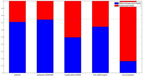
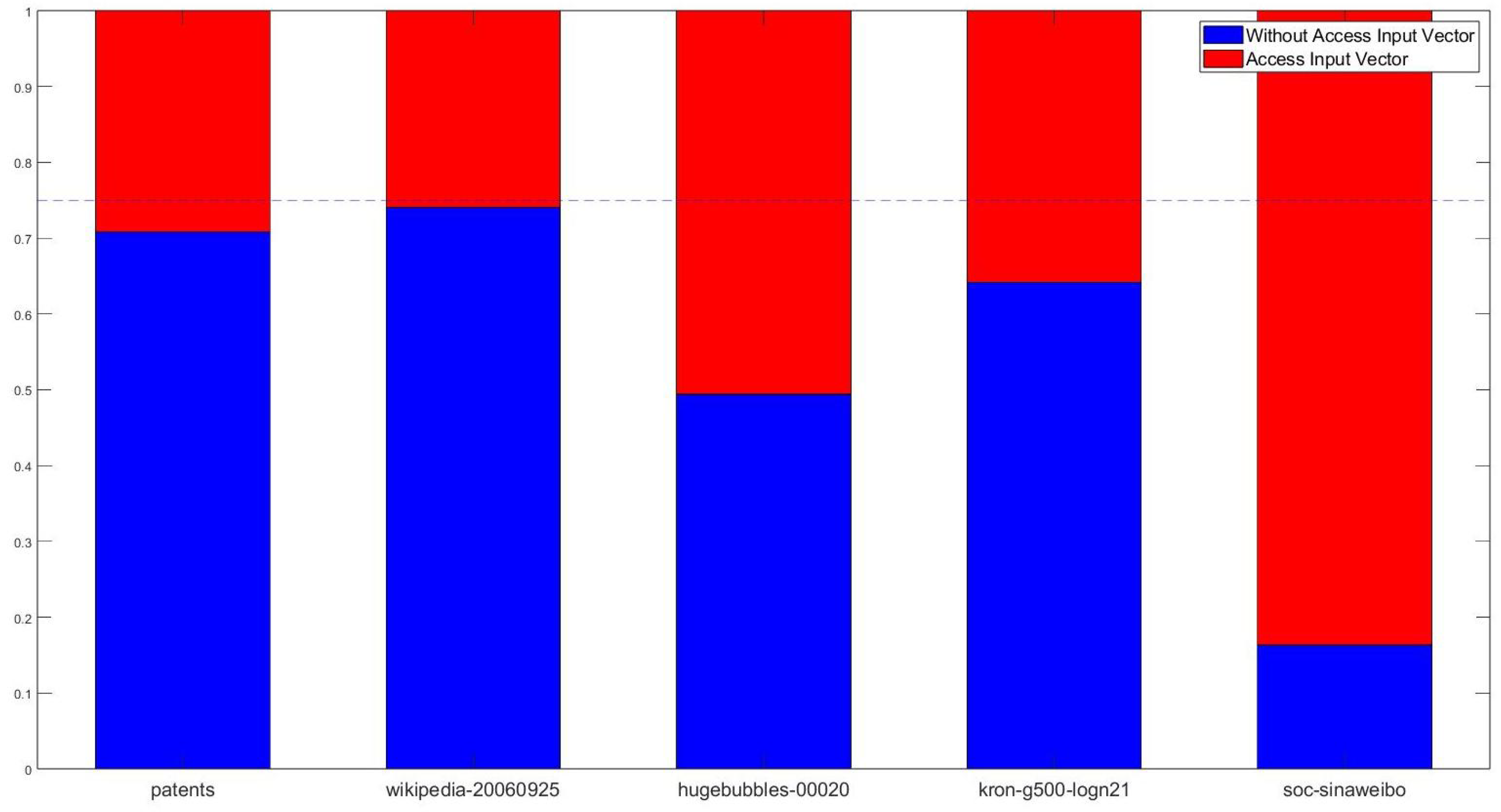
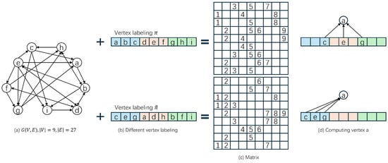
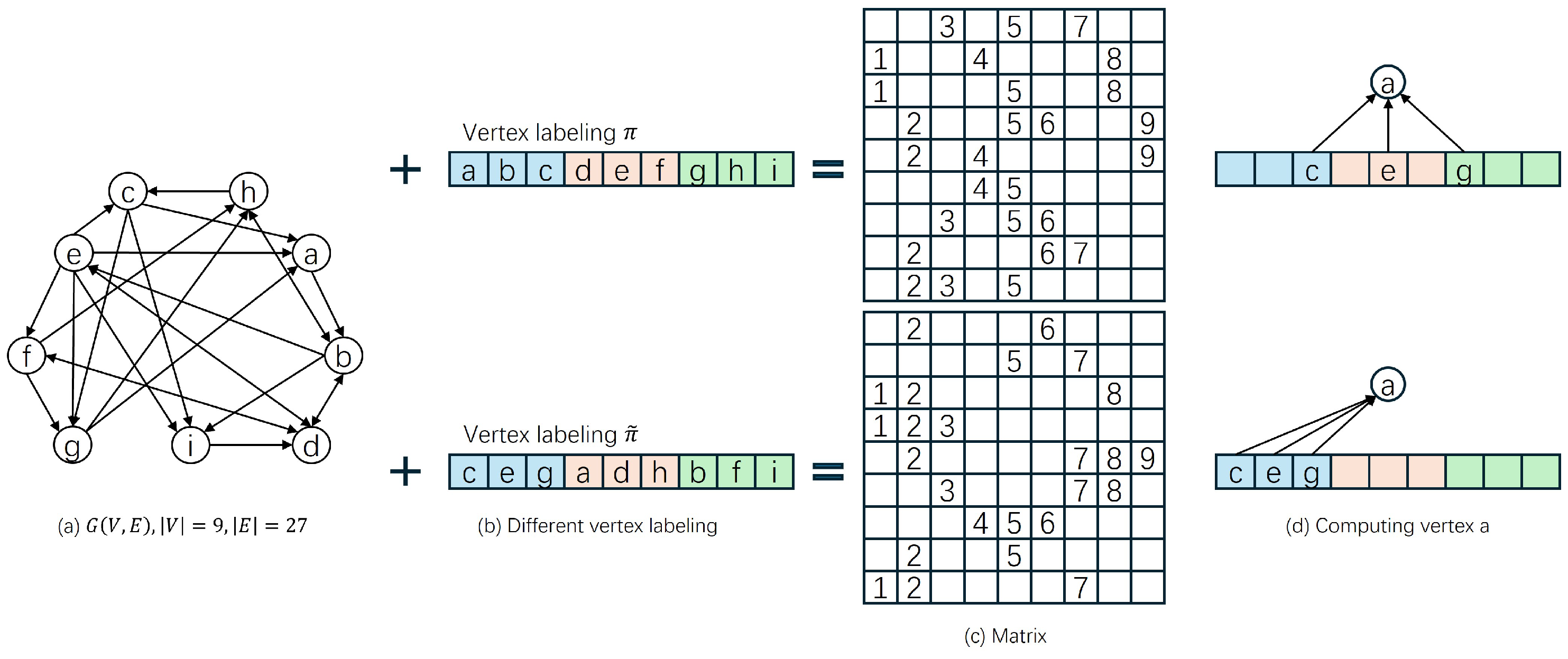
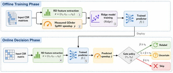
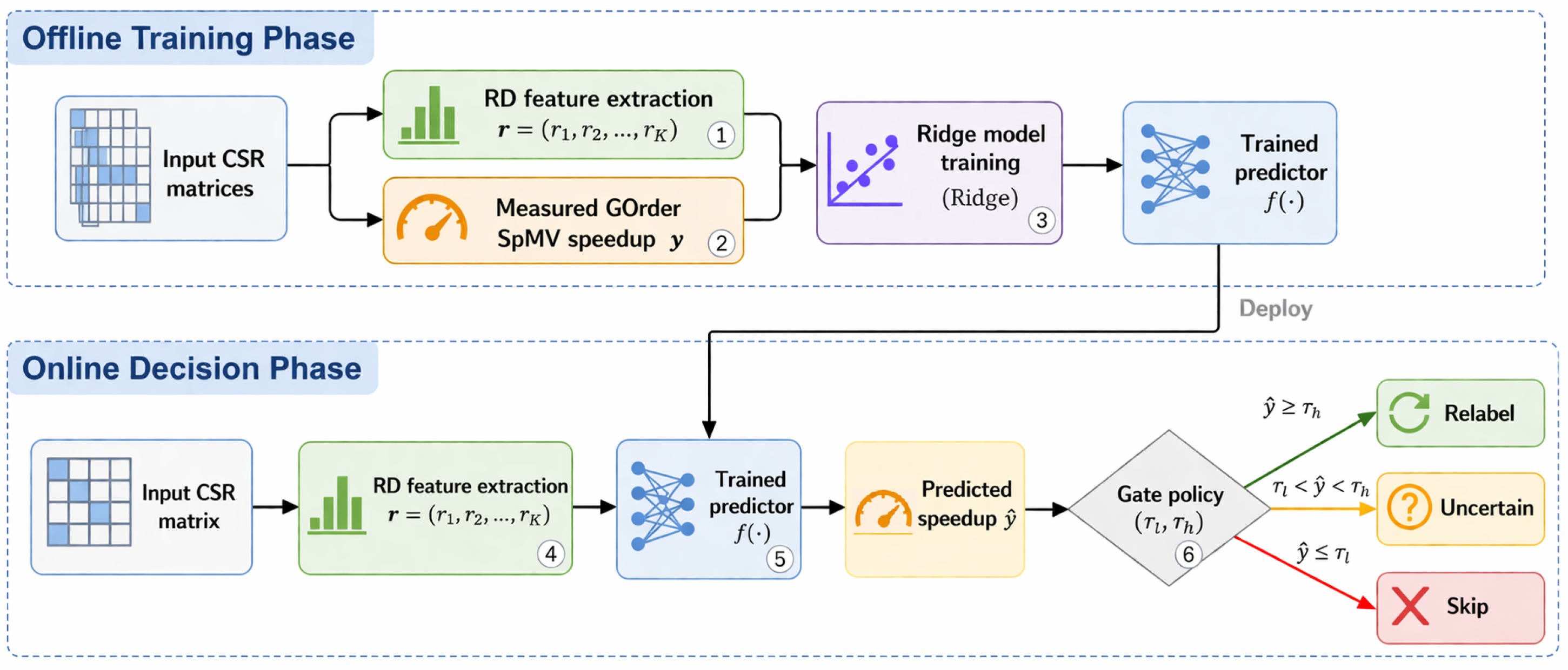
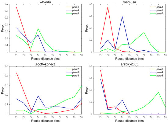
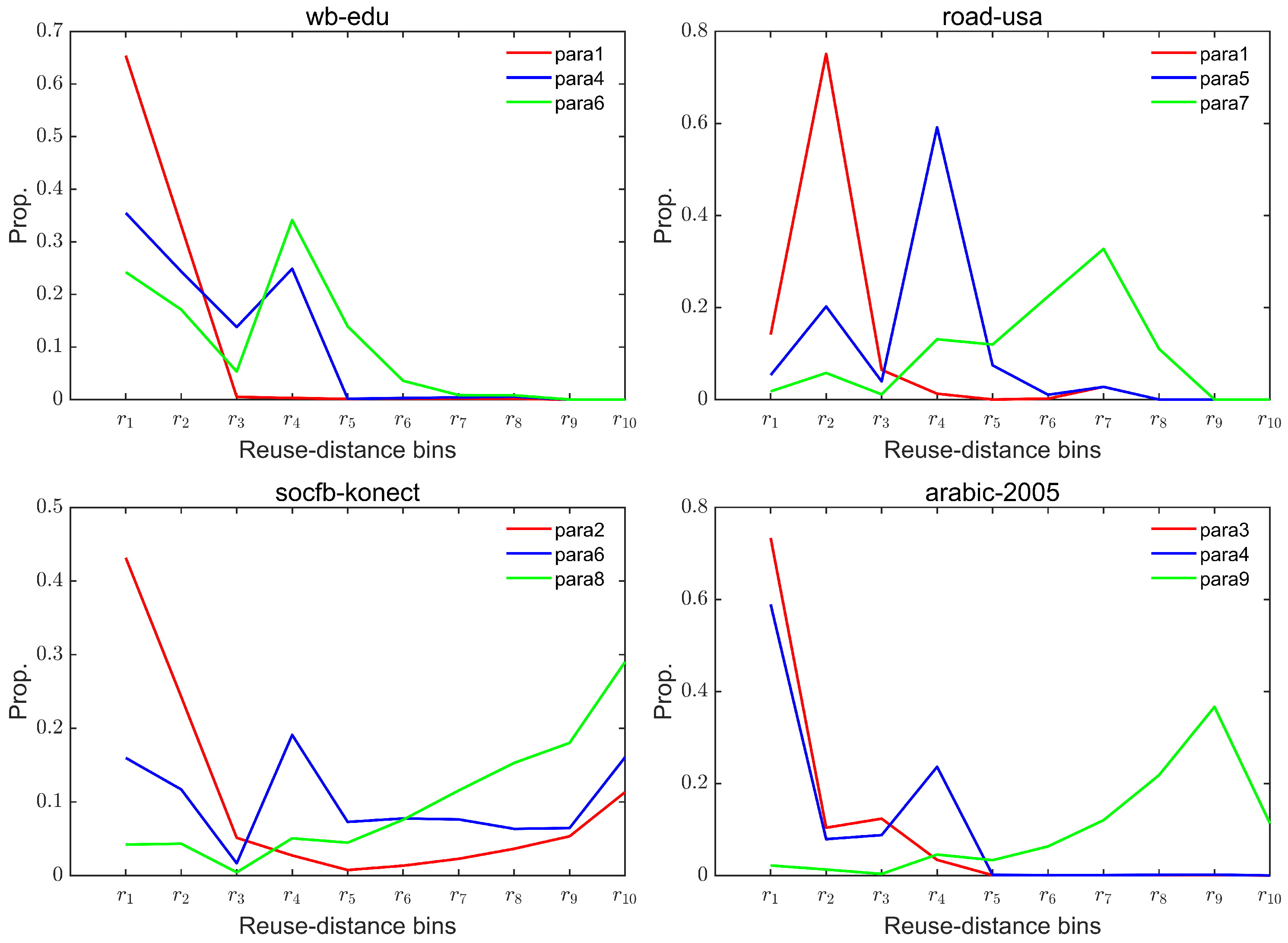
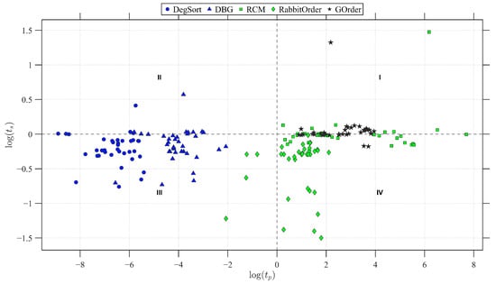
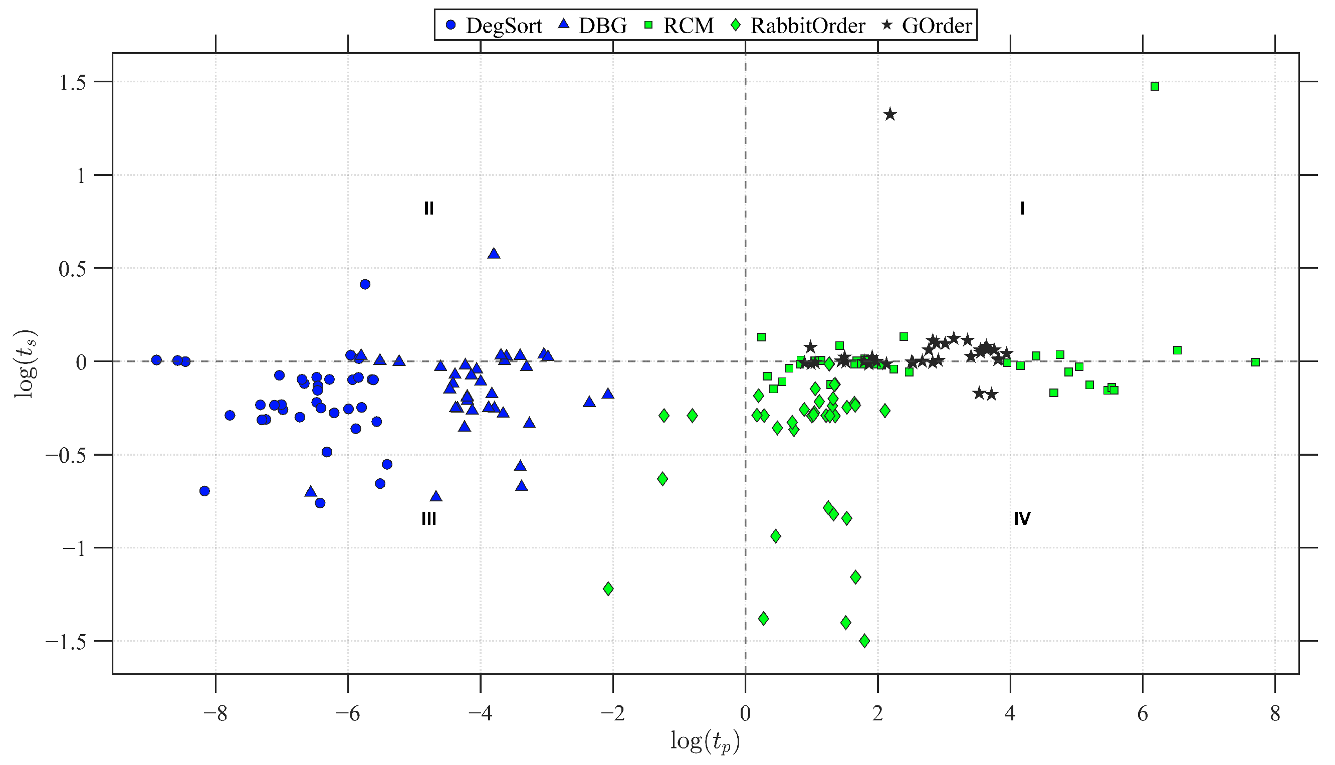
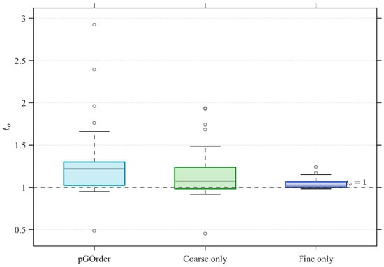
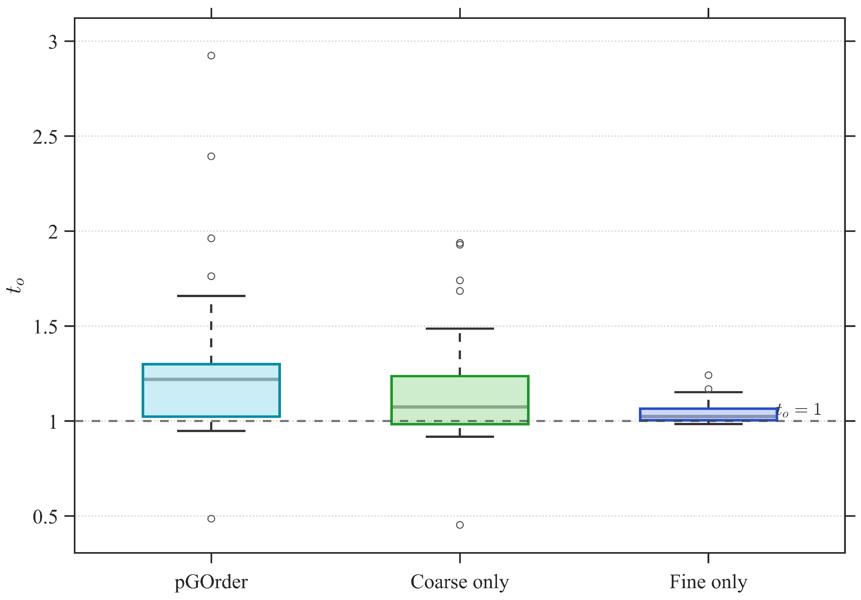
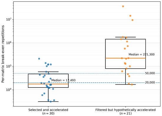
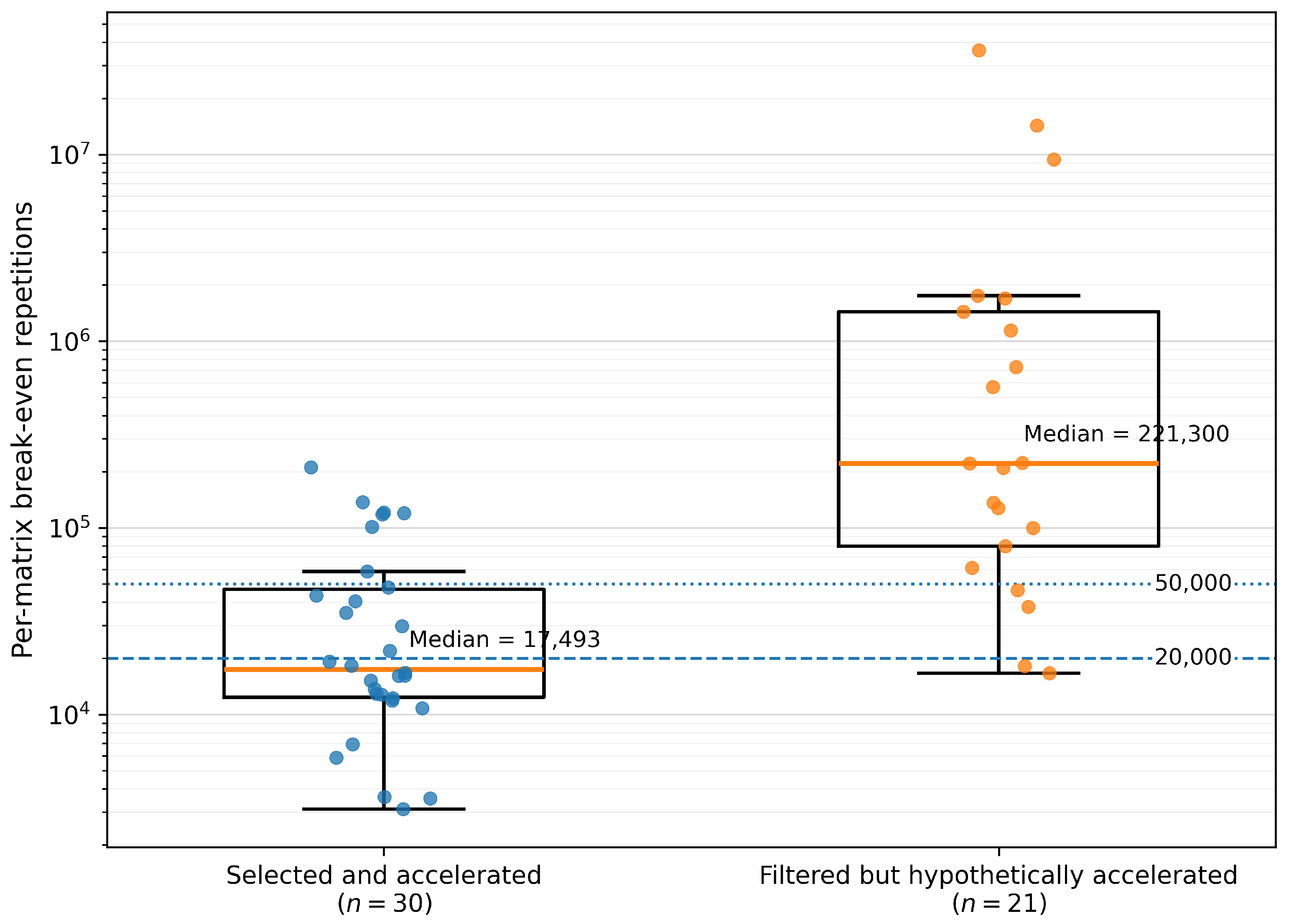

Disclaimer/Publisher’s Note: The statements, opinions and data contained in all publications are solely those of the individual author(s) and contributor(s) and not of MDPI and/or the editor(s). MDPI and/or the editor(s) disclaim responsibility for any injury to people or property resulting from any ideas, methods, instructions or products referred to in the content. |
© 2026 by the authors. Licensee MDPI, Basel, Switzerland. This article is an open access article distributed under the terms and conditions of the Creative Commons Attribution (CC BY) license.