Quartic Rational Iterations for the Matrix Sign with Applications to Principal Square Roots and Inverse Square Roots

Abstract

This paper develops a new rational fixed-point iteration for $\mathrm{sign}(M)$ whose scalar prototype enjoys half-plane global convergence and a quartic local error contraction. By embedding M into a block matrix and exploiting the classical sign–square root identity, the proposed iteration yields $M^{1/2}$ and $M^{-1/2}$ within a single iterative run under standard spectral admissibility conditions. A norm-balancing scaling strategy is also incorporated to accelerate the initial phase without changing the asymptotic order. Numerical experiments in a unified implementation demonstrate that the method reduces iteration counts and time compared with Newton-type and Padé-based competitors.

1. Introduction

A matrix function is a mathematical mapping in which the argument is a matrix, usually a square one, and the resulting value is again a matrix of the same size. Several equivalent definitions of matrix functions have been developed in the literature. Among the most common constructions are those via the Jordan canonical form, the Cauchy integral formula, and Hermite matrix polynomial representations; for further details, see [1,2]. These formulations constitute an essential theoretical and computational basis for the treatment of matrix functions in many areas of applied mathematics.

Although traditional approaches, such as diagonalization and contour-integral techniques, are frequently used for evaluating matrix functions, iterative procedures have become increasingly important. This is especially the case when the entries of the matrix vary with time or when reliable initial estimates are available [3,4]. In such circumstances, iterative schemes provide both flexibility and computational efficiency, and therefore play an important role in large-scale and real-time computations [5].

This paper is concerned with the iterative evaluation of MSRs, with particular attention to their algorithmic formulation and convergence properties. One of the main motivations behind this study comes from applications involving matrix differential equations [1]. As a simple illustration, consider the first-order matrix differential equation

$${\displaystyle \frac{d}{dt}}u(t)=\sqrt{M}u(t)+v(t),$$

(1)

where $v(t)$ is a real-valued function and $\sqrt{M}$ denotes an arbitrary square root of the matrix M. Under suitable assumptions, the exact solution of this equation can be written explicitly as

$$u(t)=\exp (t\sqrt{M})u(0)+{\int }_0^t\exp ((t-\tau )\sqrt{M})v(\tau )d\tau ,$$

(2)

which highlights the direct influence of the matrix square root (MSR) on the time evolution of the solution. Another related model is the second-order matrix differential equation

$$\left\{\begin{array}{c}{v}^{″}(t)+Mv(t)=0,\hfill \\ \\ v(0)=v_0,v^{\prime }(0)=v_0^{\prime },\hfill \end{array}\right.$$

(3)

whose vector solution is given by

$$v(t)=M^{-1/2}\sin (\sqrt{M}t)v_0^{\prime }+\cos (\sqrt{M}t)v_0.$$

(4)

MSRs also arise naturally in Monte Carlo simulation of correlated asset returns. Let $\mathsf{\Sigma }$ denote the covariance matrix of asset returns. A square root factor L, for instance obtained through the Cholesky decomposition [6], satisfies

$$\mathsf{\Sigma }=L{L}^{\top },\mathrm{where}L={\mathsf{\Sigma }}^{1/2}.$$

To generate a correlated random vector $X\sim \mathcal{M}(0,\mathsf{\Sigma })$, one can first sample a standard normal vector $Z\sim \mathcal{M}(0,I)$ and then set

$$X=LZ.$$

This operation transfers the required covariance and correlation structure to the simulated vector. Such a procedure is widely employed in multi-asset [7] derivative valuation and portfolio simulation. Beyond these classical applications, MSRs and inverse MSRs also occur in several modern computational fields. In machine learning and data analysis, the inverse square root of a covariance matrix is a central ingredient in whitening transformations and covariance normalization, where correlated features are transformed into approximately uncorrelated components with normalized variance [8]. Matrix square roots also arise in quantum information theory, for example in the computation of fidelity-type quantities between density matrices, where expressions involving the square root of positive semi-definite operators play a fundamental role [9]. These contemporary applications further motivate the development of accurate and stable algorithms for computing $M^{1/2}$ and $M^{-1/2}$, especially when the matrix dimension is large or when repeated evaluations are required.

Observing the (4), both the principal MSR and its inverse are essential components in constructing the corresponding numerical solution [10]. It should also be recalled that a square root of $M\in {\mathbb{C}}^{n\times n}$ exists iff the ascent sequence of integers $o_1,o_2,\dots$, which characterizes the sizes of the Jordan blocks associated to each eigenvalue, contains no pair of identical odd integers. This criterion was established in [11] and is expressed through

$$o_i=\dim (\mathrm{null}(M^i))-\dim (\mathrm{null}(M^{i-1})).$$

(5)

In this work, we develop a new higher-order iterative procedure for obtaining both the principal square root of a matrix and its inverse, provided that the matrix satisfies the required admissibility assumptions. It is shown that, under appropriate conditions, the proposed method globally converges to the principal square root. In addition, the convergence order of the scheme is four, which makes it an efficient approach for numerical implementation.

Before introducing the proposed method, we recall several basic facts concerning the matrix sign function, since this function is closely related to the computation of MSRs both theoretically and algorithmically. The sign function of a matrix can be defined through the following Cauchy-type integral representation:

$$\mathrm{sign}(M)=\mathsf{\Omega }={\displaystyle \frac{2}{\pi }}M{\int }_0^{\infty }{(l^{2}I+M^2)}^{-1}dl.$$

(6)

Here, the integral is interpreted within the framework of complex matrix functions, and it is assumed that M has no eigenvalues on the imaginary axis. An important point is that, although the matrix sign function satisfies $\mathrm{sign}{(M)}^2=I$, it does not necessarily coincide with either I or $-I$, unless the full spectrum of M lies strictly in the open right or left half-plane of the complex plane, respectively [12]. Therefore, the matrix sign function may be regarded as a non-primary MSR of the identity.

It is also useful to note that many mathematical problems, despite not appearing at first sight to belong to nonlinear equation theory, can be reformulated as root-finding problems in more general settings, such as spaces of operators [13,14]. The present paper is mainly focused on iterative methods in matrix computations [15]. Starting from a suitable initial matrix, such methods act as fixed-point or Newton-type processes [16,17,18], producing a sequence of matrix approximations that converges to the desired solution. Although the connection between iterative methods for the matrix sign function and classical nonlinear root solvers may not be immediately obvious, it becomes clear by observing that many sign iterations are obtained by transferring scalar root-finding ideas to the nonlinear equation [19]

$$f(x)=x^2-1=0,$$

(7)

wherein $f:D\subseteq \mathbb{C}\to \mathbb{C}$ is given. This viewpoint establishes a useful bridge between two apparently different frameworks and helps guide the construction and analysis of efficient algorithms for matrix functions.

The remainder of this article is structured as follows. Section 2 reviews several well-known iterative methods with different convergence orders for obtaining matrix functions, in particular the matrix sign function and the MSR. Section 3 presents the new iterative scheme for the simultaneous computation of the MSR and its inverse. In that section, we discuss the mathematical formulation of the method, its relation to the matrix sign function, and the derivation of its global convergence properties. The convergence rate of the presented iteration is also examined in detail. Section 4 investigates the computational performance of the method through a collection of numerical experiments on test matrices of arbitrary dimensions, thereby confirming the theoretical results. Finally, Section 5 summarizes the main conclusions and indicates possible directions for future work.

2. Review of Classic Iterative Schemes

By applying the standard Newton method to matrixeq), one obtains the classical solver for computing the matrix sign function, as described in [10]:

$$U_{j+1}={\displaystyle \frac{1}{2}}\left(U_j+U_j^{-1}\right).$$

(8)

Here, $\{U_j\}$ represents the sequence of matrix approximations produced by the iterative process. A classical approach for computing a MSR is also furnished by Newton’s method, which can be expressed in the recursive form

$$U_{j+1}={\displaystyle \frac{1}{2}}\left[U_j+M{U}_j^{-1}\right],$$

(9)

where $U_0$ is a suitably chosen starting matrix. Although the iteration in (9) is attractive from a theoretical point of view, it may suffer from numerical instability, especially when the initial approximation $U_0$ is not properly selected or when the matrix M has structural properties that adversely affect the convergence process.

To overcome such drawbacks and to obtain better stability together with improved convergence behavior, several modified iterations have been proposed in the literature [20]. One such second-order scheme, developed from the Newton iteration in (9), was introduced in [20] and is given by

$$\left\{\begin{array}{c}{Z}_0=I,U_0=M,j=0,1,\cdots ,\hfill \\ U_{j+1}={\displaystyle \frac{1}{2}}[U_j+Z_j^{-1}],\hfill \\ Z_{j+1}={\displaystyle \frac{1}{2}}[Z_j+U_j^{-1}].\hfill \end{array}\right.$$

(10)

The process defined in (10) is known to possess favorable numerical stability properties, and the sequence $\{U_j\}$ produced by this scheme tends to the principal MSR of M, denoted by $M^{1/2}$.

Another well-known technique for evaluating MSRs is obtained from the cyclic reduction algorithm, originally proposed in [21]:

$$\left\{\begin{array}{c}{Z}_0=2(I+M),U_0=I-M,j=0,1,\cdots ,\hfill \\ U_{j+1}=-U_j{Z}_j^{-1}{U}_j,\hfill \\ Z_{j+1}=Z_j-2U_j{Z}_j^{-1}{U}_j.\hfill \end{array}\right.$$

(11)

This method constructs a sequence $\{Z_j\}$ that asymptotically tends to $4M^{1/2}$. Hence, although the iteration converges to a scaled form of the desired square root, the principal MSR $M^{1/2}$ is recovered by applying the corresponding normalization to the final approximation.

Padé-Based Competitor Solvers for the Matrix Sign Function

An important family of optimal iterations for computing the matrix sign function was developed in [22]. These schemes are obtained by using Padé approximants of the scalar function

$$f(\zeta )={\displaystyle \frac{1}{\sqrt{1-\zeta }}},$$

together with the change of variable $\zeta =1-u^2$. This construction produces a class of rational functions that form the basis of the Padé-type sign iterations. Owing to their optimality properties and favorable numerical stability, these methods are regarded as strong competitors among iterative techniques for matrix function computation. The resulting rational iterations exhibit rapid convergence to the sign function and arise from the identity

$$\mathrm{sign}(u)=s={\displaystyle \frac{u}{{(u^2)}^{1/2}}}={\displaystyle \frac{u}{{(1-\zeta )}^{1/2}}}.$$

(12)

Assume that ${\kappa }_1+{\kappa }_2\ge 1$, and let the $[{\kappa }_1,{\kappa }_2]$ Padé approximant of $f(\xi )$ be denoted by ${\displaystyle \frac{P_{{\kappa }_1,{\kappa }_2}(\xi )}{Q_{{\kappa }_1,{\kappa }_2}(\xi )}}$. Then, one obtains the iteration

$$u_{j+1}={\displaystyle \frac{u_j{P}_{{\kappa }_1,{\kappa }_2}(1-u_j^2)}{Q_{{\kappa }_1,{\kappa }_2}(1-u_j^2)}}:={\phi }_{2{\kappa }_1+1,2{\kappa }_2},$$

(13)

which converges to $\pm 1$ with order $1+{\kappa }_1+{\kappa }_2$. In this Padé framework, the symbols P and Q denote the numerator and denominator polynomials of the corresponding Padé approximant, respectively.

Generally speaking, the iterations represented by (13), together with their reciprocal variants, are obtained from the $[{\kappa }_1/{\kappa }_1]$ and $[({\kappa }_1-1)/{\kappa }_1]$ Padé approximants of the underlying function. These classes of schemes are globally convergent. Furthermore, the convergence behavior of each method depends on the selected Padé indices, which determine the degree of the associated rational approximation; see also [23].

Within this Padé-based class, some iterations attain fourth-order convergence while retaining global stability for a wide range of input matrices. Typical examples of globally convergent fourth-order schemes are listed as follows:

$$U_{j+1}=[I+6U_j^2+U_j^4]{[4U_j(I+U_j^2)]}^{-1},\mathrm{Padé}\text{-}\mathrm{type}(1,2)\mathrm{iteration},$$

(14)

$$U_{j+1}=[4U_j(I+U_j^2)]{[I+6U_j^2+U_j^4]}^{-1},\mathrm{reciprocal}\mathrm{Padé}\text{-}\mathrm{type}(1,2)\mathrm{iteration}.$$

(15)

3. An Enhanced Approach

3.1. Construction of an Improved Scheme

To enhance the accuracy and convergence behavior of Newton’s scheme [24], we add a supplementary correction step based on a divided-difference approximation. This modification gives rise to an enhanced iterative algorithm for solving the nonlinear equation in (7):

$$\begin{array}{c}\hfill \left\{\begin{array}{c}{y}_j=t_j-{\displaystyle \frac{f(t_j)}{f^{\prime }(t_j)}},t_0\ge 0,\hfill \\ h_j=t_j-{\displaystyle \frac{(t_j-1)(t_j+1)\left(297t_j^2+103\right)}{394t_j^3+406t_j}},\hfill \\ t_{j+1}=h_j-{\displaystyle \frac{f(h_j)}{f[h_j,t_j]}},\hfill \end{array}\right.\end{array}$$

(16)

wherein $f[c_1,c_2]:={(c_1-c_2)}^{-1}(f(c_1)-f(c_2))$. Throughout this subsection, $t_j$, $y_j$, and $h_j$ are scalar variables. When the method is transferred to the matrix sign problem, their corresponding matrix iterates will be denoted by capital letters.

The iteration in (16) is designed with two main objectives. The first is to improve the classical Newton process by increasing the convergence order. The second, which is even more important for matrix computations, is to obtain a formulation with global convergence characteristics. Hence, the proposed construction combines high local efficiency with global stability, making it suitable for nonlinear matrix problems where both reliability and computational performance are essential.

Theorem 1.

Let $x^{*}\in D$ be a simple zero of a sufficiently differentiable function $f:D\subseteq \mathbb{C}\to \mathbb{C}$. If the initial point $t_0$ is selected close enough to the exact zero $x^{*}$, then the method defined by (16) satisfies the error relation

$${\vartheta }_{j+1}=\left(-{\displaystyle \frac{d_2^3}{1000}}\right){\vartheta }_j^4+\mathcal{O}({\vartheta }_j^5),$$

(17)

where ${\vartheta }_j=t_j-x^{*}$ and $d_i={\displaystyle \frac{f^{(i)}(x^{*})}{i!f^{\prime }(x^{*})}}$, $i\ge 2$.

Proof. 

Expanding the relevant terms around $x^{*}$ by Taylor’s formula gives

$${\displaystyle \frac{f(t_j)}{f^{\prime }(t_j)}}={\vartheta }_j-d_2{\vartheta }_j^2+\left(2d_2^2-2d_3\right){\vartheta }_j^3+\left(-4d_2^3+7d_2{d}_3-3d_4\right){\vartheta }_j^4+\mathcal{O}({\vartheta }_j^5).$$

(18)

Therefore, using the first step of (16), we obtain

$$y_j-x^{*}=d_2{\vartheta }_j^2+\left(-2d_2^2+2d_3\right){\vartheta }_j^3+\left(4d_2^3-7d_2{d}_3+3d_4\right){\vartheta }_j^4+\mathcal{O}({\vartheta }_j^5).$$

(19)

For the second stage of (16), expanding the rational Newton-type correction about $x^{*}$ and inserting the Taylor coefficients of f and $f^{\prime }$ leads to the third-order error representation

$$h_j-x^{*}={\gamma }_3{\vartheta }_j^3+{\gamma }_4{\vartheta }_j^4+\mathcal{O}({\vartheta }_j^5),$$

(20)

where

$${\gamma }_3=-{\displaystyle \frac{d_2^2}{1000}}.$$

(21)

For the divided difference appearing in (16), we have $f[h_j,t_j]={\displaystyle \frac{f(h_j)-f(t_j)}{h_j-t_j}}$. By expanding $f(h_j)$ and $f(t_j)$ around $x^{*}$ and then using (20), it follows that

$$f[h_j,t_j]=f^{\prime }(x^{*})\left(1+d_2{\vartheta }_j+\mathcal{O}({\vartheta }_j^2)\right),{\displaystyle \frac{1}{f[h_j,t_j]}}={\displaystyle \frac{1}{f^{\prime }(x^{*})}}\left(1-d_2{\vartheta }_j+\mathcal{O}({\vartheta }_j^2)\right).$$

(22)

Moreover, since $h_j-x^{*}=\mathcal{O}({\vartheta }_j^3)$, we also have

$${\displaystyle \frac{f(h_j)}{f^{\prime }(x^{*})}}=(h_j-x^{*})+\mathcal{O}\left({(h_j-x^{*})}^2\right)=(h_j-x^{*})+\mathcal{O}({\vartheta }_j^5).$$

(23)

Combining (22) and (23) gives

$${\displaystyle \frac{f(h_j)}{f[h_j,t_j]}}=(h_j-x^{*})\left(1-d_2{\vartheta }_j+\mathcal{O}({\vartheta }_j^2)\right).$$

Consequently, from the last step of (16) together with (21), we arrive at

$$\begin{array}{cc}\hfill t_{j+1}-x^{*}& =(h_j-x^{*})-{\displaystyle \frac{f(h_j)}{f[h_j,t_j]}}=(h_j-x^{*})\left(d_2{\vartheta }_j+\mathcal{O}({\vartheta }_j^2)\right)\hfill \\ \hfill & =\left(-{\displaystyle \frac{d_2^2}{1000}}{\vartheta }_j^3+\mathcal{O}({\vartheta }_j^4)\right)\left(d_2{\vartheta }_j+\mathcal{O}({\vartheta }_j^2)\right)=-{\displaystyle \frac{d_2^3}{1000}}{\vartheta }_j^4+\mathcal{O}({\vartheta }_j^5),\hfill \end{array}$$

(24)

which proves (17). □

3.2. Extension to the Sign Function

Applying (16) to the nonlinear Equation (7) and extending the resulting scalar iteration to matrices in a direct manner yields the following high-order method for computing the matrix sign function:

$$U_{j+1}=U_j\left(509I+994U_j^2+97U_j^4\right){\left[103I+1006U_j^2+491U_j^4\right]}^{-1},$$

(25)

where the initial matrix is chosen for a nonsingular square complex matrix as

$$U_0=M.$$

(26)

By using the same construction, one may also write the reciprocal counterpart in the form

$$U_{j+1}=\left(103I+1006U_j^2+491U_j^4\right){\left[U_j\left(509I+994U_j^2+97U_j^4\right)\right]}^{-1}.$$

(27)

It should be stressed that the efficiency of an iterative method cannot be judged solely from its convergence order. The computational work required at each step is also a decisive factor, since it affects the total cost of the algorithm. Comparing the iterations in (25) and (27) with the Padé-based schemes in (14) and (15) shows that all these methods require 4 matrix–matrix multiplications and one linear solve, equivalently one inverse factor in compact mathematical notation, per iteration. Thus, the new schemes in (25)–(27) form competitive alternatives to the Padé iterations of the same convergence order, while also retaining global convergence properties.

Remark 1.

Although the iterations (25) and (27) are written with inverse notation, this notation should be understood as a compact mathematical representation rather than as a recommendation to explicitly compute matrix inverses. In practical implementations, the inverse factor should be avoided. For instance, in (27), define

$$N_j=103I+1006U_j^2+491U_j^4,D_j=U_j\left(509I+994U_j^2+97U_j^4\right).$$

Then (27) may be written as

$$U_{j+1}=N_j{D}_j^{-1}.$$

Instead of forming $D_j^{-1}$, one should compute $U_{j+1}$ as the solution of the right linear matrix equation

$$U_{j+1}{D}_j=N_j.$$

Equivalently, this can be implemented by solving the transposed system

$$D_j^{\top }{U}_{j+1}^{\top }=N_j^{\top }.$$

In dense matrix computations, this system can be solved by LU factorization with partial pivoting, while for structured or sparse matrices one may use a factorization or Krylov-type linear solver adapted to the matrix structure. The same convention is used for the other inverse factors appearing in the competing schemes. Therefore, the stated cost of one matrix inversion per iteration should be interpreted in the standard numerical-linear-algebra sense as one linear solve with the corresponding coefficient matrix.

3.3. Convergence over the Entire Domain for Matrix Sign

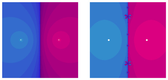
To investigate the global nature of convergence, we employ the concept of basins of attraction [25]. This tool provides both graphical and theoretical information about the regions in which an iterative method converges [26]. More precisely, we take into account the complex domain $[-2,2]\times [-2,2]\subset \mathbb{C}$ and discretize it into a sufficiently fine grid. Each grid point is used as an initial approximation, and the point is colored according to the root to which the iteration converges. Points that fail to converge are displayed in black. The stopping rule used in this experiment is $|f(x_j)| \le {10}^{-6}$.

The corresponding graphical results are reported in Figure 1 and Figure 2. In these figures, the intensity of the color indicates the number of iterations required to satisfy the convergence criterion. To provide a comparison, some Padé-based competitor schemes are also included, so that the distinction between local and global convergence behavior can be observed.

Figure 1. Attraction basins for (9) in left and Padé 1–4 in right.

Figure 2. Attraction basins for (25) in left and (27) in right.

Although the iterations (9), (27), and (14) all display global convergence, a more careful comparison of their attraction basins shows a clear advantage for the scheme (27). In particular, the lighter regions associated with this method indicate that fewer iterations are generally required to reach convergence. This improvement is especially meaningful because all compared methods have the same per-step computational cost in terms of the number of matrix products and matrix inversions.

Theorem 2.

Let $\varphi :\mathbb{C}\setminus \{0\}\setminus \{z:509+994z^2+97z^4=0\}\to \mathbb{C}$ be the rational mapping generated by (27), namely

$$\varphi (z)={\displaystyle \frac{103+1006z^2+491z^4}{z\left(509+994z^2+97z^4\right)}}.$$

(28)

Consider the fixed-point process

$$t_{j+1}=\varphi (t_j),j=0,1,\dots$$

(29)

Then, for every initial value $t_0\in \mathbb{C}$ satisfying $\mathcal{R}(t_0)\ne 0$, the sequence $\{t_j\}$ is well-defined and converges globally to the corresponding solution of $t^2-1=0$; that is,

$$\mathcal{R}(t_0)>0⟹t_j\to 1,\mathcal{R}(t_0)<0⟹t_j\to -1.$$

The exceptional set is the imaginary axis $\{t_0:\mathcal{R}(t_0)=0\}$, which constitutes the common boundary of the two attraction regions.

Proof. 

Let $s\in \{+1,-1\}$ be selected so that $\mathcal{R}(s{t}_0)>0$; equivalently, $s=1$ when $\mathcal{R}(t_0)>0$ and $s=-1$ when $\mathcal{R}(t_0)<0$. Define the Cayley transform

$${\omega }_j={\displaystyle \frac{t_j-s}{t_j+s}}.$$

(30)

The equivalence

$$\mathcal{R}(sz)>0⟺\left|{\displaystyle \frac{z-s}{z+s}}\right|<1$$

(31)

implies that $\mathcal{R}(s{t}_0)>0$ gives $|{\omega }_0| <1$.

A direct simplification of (28) yields the exact recurrence

$${\omega }_{j+1}=-{\omega }_j^4{\displaystyle \frac{97t_j-103s}{97t_j+103s}}.$$

(32)

Furthermore, for every $z\in \mathbb{C}$ and $s\in \{\pm 1\}$, one has

$${|97z+103s|}^2-{|97z-103s|}^2=4·97·103\mathcal{R}(sz),$$

and therefore $\mathcal{R}(sz)>0$ implies

$$\left|{\displaystyle \frac{97z-103s}{97z+103s}}\right|<1.$$

(33)

If $|{\omega }_j| <1$, then (31) gives $\mathcal{R}(s{t}_j)>0$, so that (33) is applicable with $z=t_j$. Taking absolute values in (32), we get

$$|{\omega }_{j+1}| = |{\omega }_j{|}^4\left|{\displaystyle \frac{97t_j-103s}{97t_j+103s}}\right|<{|{\omega }_j|}^4.$$

(34)

It follows that $|{\omega }_0| <1$ implies $|{\omega }_j| <1$ for every j, and the inequality $|{\omega }_{j+1}| < |{\omega }_j{|}^4$ forces $|{\omega }_j| \to 0$. By (30), the relation ${\omega }_j\to 0$ is equivalent to $t_j\to s$. This proves global convergence to $s\in \{+1,-1\}$ for all initial values with $\mathcal{R}(t_0)\ne 0$. Finally, when $\mathcal{R}(t_0)=0$, Equation (31) gives $|{\omega }_0| =1$, and hence the strict contraction argument above is no longer valid. The imaginary axis is therefore exactly the boundary separating the attraction basins of $+1$ and $-1$. This completes the proof. □

3.4. Computation of the MSR

To adapt the iteration in (25) to the computation of MSRs, we use the following key identity, given in [1]:

$$\mathrm{sign}(\mathbf{M})=\mathrm{sign}\left(\left[\begin{array}{cc}0& M\\ I& 0\end{array}\right]\right)=\left[\begin{array}{cc}0& M^{1/2}\\ M^{-1/2}& 0\end{array}\right].$$

(35)

If M is nonsingular and $\sigma (M)\cap {\mathbb{R}}^{-}=\varnothing$, then the block matrix $\mathbf{M}=\left[\begin{array}{cc}0& M\\ I& 0\end{array}\right]$ satisfies $\sigma (\mathbf{M})\cap i\mathbb{R}=\varnothing$. Hence, $\mathrm{sign}(\mathbf{M})$ is well-defined, and (35) simultaneously provides $M^{1/2}$ and $M^{-1/2}$. This relation creates the essential link between the matrix sign function and the MSR problem. In particular, it converts the computation of the MSR into the evaluation of a matrix sign function by embedding the original matrix into the block matrix $\mathbf{M}\in {\mathbb{C}}^{2n\times 2n}$.

Another relevant structural property of the proposed iterations should also be noted when they are applied to a nonsingular matrix M whose spectrum avoids the negative real axis, that is, when M has no eigenvalues on ${\mathbb{R}}^{-}$, [27]. Under this condition, assume that the initial approximation $U_0$ is chosen to commute with M, namely $M{U}_0=U_{0}M$. Then, by induction, every subsequent iterate generated by the method preserves this commutativity. Thus, each matrix $U_j$ satisfies $M{U}_j=U_{j}M$, meaning that the iteration remains consistent with the spectral structure of M during the entire convergence process. This invariance is useful for numerical stability and also simplifies the theoretical analysis of the MSR computation.

3.5. Error Estimate and Convergence Order

Theorem 3.

Let M be nonsingular with $\sigma (M)\cap i\mathbb{R}=\varnothing$ and take $U_0=M$. Then, the iteration (27) converges to $\mathsf{\Omega }=\mathrm{sign}(M)$ with fourth-order convergence.

Proof. 

We establish quartic convergence to $\mathsf{\Omega }=\mathrm{sign}(M)$ for the initial choice $U_0=M$. The corresponding conclusions for the MSR and $M^{-1/2}$ are obtained by applying the same sign iteration to the block matrix in (35). Recall that every complex square matrix M, whether diagonalizable or defective, can be represented in Jordan form as $M=TJ{T}^{-1}$, where T is nonsingular and J is composed of Jordan blocks associated with the eigenvalues of M. This decomposition allows the convergence analysis of the iteration to be reduced to the behavior on individual Jordan blocks.

In this transformed setting, the eigenvalues of the iterates, denoted by ${\alpha }_j$, can be followed through a scalar recurrence that describes the passage from step j to step $j+1$. Let ${\lambda }_i\in \sigma (M)$, $1\le i\le n$, and define

$$s_i=\mathrm{sign}({\lambda }_i)\in \{+1,-1\},\mathrm{sign}({\lambda }_i)=\left\{\begin{array}{cc}+1,\hfill & \mathcal{R}({\lambda }_i)>0,\hfill \\ -1,\hfill & \mathcal{R}({\lambda }_i)<0,\hfill \end{array}\right.$$

which is meaningful because of the assumption $\sigma (M)\cap i\mathbb{R}=\varnothing$. Since (27) is rational, each iterate is a rational function of $U_0$, and hence of M. Therefore, the spectral mapping theorem applies. In particular, if ${\alpha }_j^i\in \sigma (U_j)$ denotes the eigenvalue corresponding to ${\lambda }_i$ with algebraic multiplicity taken into account, then the scalar iteration induced by (27) is

$${\alpha }_{j+1}^i={\displaystyle \frac{103+1006{({\alpha }_j^i)}^2+491{({\alpha }_j^i)}^4}{{\alpha }_j^i\left(509+994{({\alpha }_j^i)}^2+97{({\alpha }_j^i)}^4\right)}},1\le i\le n.$$

(36)

Introduce the Cayley-type quantity

$${\omega }_j^i:={\displaystyle \frac{{\alpha }_j^i-s_i}{{\alpha }_j^i+s_i}}.$$

(37)

A direct algebraic simplification of the scalar map in (36), using $s_i^2=1$, gives

$${\omega }_{j+1}^i=-{\left({\omega }_j^i\right)}^4{\displaystyle \frac{97{\alpha }_j^i-103s_i}{97{\alpha }_j^i+103s_i}},1\le i\le n.$$

(38)

Taking absolute values in (38) yields

$$\left|{\omega }_{j+1}^i\right|={\left|{\omega }_j^i\right|}^4\left|{\displaystyle \frac{97{\alpha }_j^i-103s_i}{97{\alpha }_j^i+103s_i}}\right|.$$

(39)

Also, for any $z\in \mathbb{C}$ and $s\in \{\pm 1\}$, the identity

$${|97z+103s|}^2-{|97z-103s|}^2=4·97·103\mathcal{R}(sz),$$

implies

$$\mathcal{R}(sz)>0⟹\left|{\displaystyle \frac{97z-103s}{97z+103s}}\right|<1.$$

(40)

Since $\mathcal{R}(s_i{\lambda }_i)>0$ by the definition of $s_i$, and since ${\alpha }_0^i={\lambda }_i$ for $U_0=M$, it follows from (36) by induction that $\mathcal{R}(s_i{\alpha }_j^i)>0$ for all j. Thus, the multiplicative factor in (39) is always strictly smaller than 1. Consequently, $\{|{\omega }_j^i|\}$ decreases monotonically and satisfies a fourth-order superlinear contraction. Hence,

$$\underset{j\to \infty }{\lim }{\omega }_j^i=0,\mathrm{equivalently}\underset{j\to \infty }{\lim }\left|{\displaystyle \frac{{\alpha }_j^i-s_i}{{\alpha }_j^i+s_i}}\right|=0.$$

To identify the convergence order at the matrix level, set $D_j=U_j(509I+994U_j^2+97U_j^4)$. Since $U_0=M$, every $U_j$ is a rational function of M; therefore, $U_j\mathsf{\Omega }=\mathsf{\Omega }{U}_j$. Thus, the following factorization is valid, where $sign(M)=\mathsf{\Omega }$:

$$\begin{array}{ccc}{U}_{j+1}-\mathsf{\Omega }\hfill & =\hfill & (103I+1006U_j^2+491U_j^4)D_j^{-1}-\mathsf{\Omega }\hfill \\ \hfill & =\hfill & [103I+1006U_j^2+491U_j^4-\mathsf{\Omega }{D}_j]D_j^{-1}\hfill \\ \hfill & =\hfill & [103I+1006U_j^2+491U_j^4-509U_j\mathsf{\Omega }-994U_j^3\mathsf{\Omega }-97U_j^5\mathsf{\Omega }]D_j^{-1}\hfill \\ \hfill & =\hfill & [-103(U_j-\mathsf{\Omega }{)}^4+97U_j\mathsf{\Omega }(U_j-\mathsf{\Omega }{)}^4]D_j^{-1}\hfill \\ \hfill & =\hfill & (U_j-\mathsf{\Omega }{)}^4[-103I+97U_j\mathsf{\Omega }]D_j^{-1}.\hfill \end{array}$$

(41)

Taking an appropriate matrix norm in (41) immediately gives

$$\parallel U_{j+1}-\mathsf{\Omega }\parallel \le \left(\parallel D_j^{-1}\parallel \parallel -103I+97U_j\mathsf{\Omega }\parallel \right)\parallel U_j-\mathsf{\Omega }{\parallel }^4,$$

(42)

which verifies that the method in (27) converges with order four. The proof is complete. □

The preceding convergence argument is spectral in nature and is valid under the stated admissibility assumptions. In finite-precision arithmetic, however, highly non-normal matrices may exhibit transient behavior that is not fully described by eigenvalues alone, since their pseudospectra can be much larger than their spectra. For this reason, the numerical section also includes a Jordan-type non-normal test matrix in Example 3, where the iteration history is reported explicitly to monitor possible transient growth.

3.6. Scaling

It is well known that iterative algorithms for matrix functions [28] may converge slowly during the first few iterations. This behavior is often caused by an initial approximation that is not adequately close to the desired matrix function. A common remedy for this difficulty is the use of scaling, which can considerably accelerate the early stage of convergence.

The scaling idea has been discussed in detail in ([1], Chapter 5.5), especially for Newton-type iterations. Its main purpose is to modify the current iterate dynamically by means of a scalar scaling factor. Instead of applying the iterative update directly to $U_j$, one first replaces it by ${\lambda }_j{U}_j$, where ${\lambda }_j$ is determined adaptively during the computation. This adjustment improves stability and may substantially speed up convergence when the starting matrix is not close to the required limit.

In practice, such a strategy often produces better numerical behavior and can reduce the number of iterates needed to satisfy a prescribed tolerance. For rational sign iterations, including (27), the convergence rate is controlled by the proximity of the spectrum to $\{\pm 1\}$. Equivalently, it depends on the magnitude of the Cayley-type expression

$$\omega (z)={\displaystyle \frac{z-s}{z+s}},s=\mathrm{sign}(\mathcal{R}(z))\in \{\pm 1\},$$

(43)

because the scalar map associated with (27) satisfies a contraction relation of the form

$$|\omega (\varphi (z))|\le {|\omega (z)|}^4·\Theta (z),\Theta (z)<1\mathrm{whenever}\mathcal{R}(sz)>0,$$

and the corresponding matrix statement follows from spectral mapping. Thus, any preliminary transformation that decreases $|\omega (\lambda )|$ for $\lambda \in \sigma (U_j)$ improves the initial convergence behavior.

Accordingly, at the jth step we replace $U_j$ by the scaled matrix ${\tilde{U}}_j={\lambda }_j{U}_j$ before carrying out the rational update. For a scalar z satisfying $\mathcal{R}(sz)>0$, the function $\lambda \mapsto \left|{\displaystyle \frac{\lambda z-s}{\lambda z+s}}\right|$ is minimized when $|\lambda z|$ is close to 1. In the matrix setting, a practical substitute is to balance the sizes of ${\tilde{U}}_j$ and ${\tilde{U}}_j^{-1}$ in the selected norm, namely

$$\parallel {\tilde{U}}_j\parallel \approx \parallel {\tilde{U}}_j^{-1}\parallel .$$

(44)

Since $\parallel {\tilde{U}}_j\parallel ={\lambda }_j\parallel U_j\parallel$ and $\parallel {\tilde{U}}_j^{-1}\parallel ={\lambda }_j^{-1}\parallel U_j^{-1}\parallel$, condition (44) implies

$${\lambda }_j^2={\displaystyle \frac{\parallel U_j^{-1}\parallel }{\parallel U_j\parallel }},\mathrm{hence}{\lambda }_j={\left({\displaystyle \frac{\parallel U_j^{-1}\parallel }{\parallel U_j\parallel }}\right)}^{1/2}.$$

For a higher-order sign iteration such as (27), the update contains odd powers up to $U_j^5$, and therefore an overly strong scaling may have a more pronounced effect. A customary stabilization is to employ a tempered balancing strategy, which enforces (44) at the squared-magnitude level. This gives

$$\parallel {\lambda }_j^2{U}_j\parallel \approx \parallel {({\lambda }_j^2{U}_j)}^{-1}\parallel ⟹{\lambda }_j^4={\displaystyle \frac{\parallel U_j^{-1}\parallel }{\parallel U_j\parallel }}⟹{\lambda }_j={\left({\displaystyle \frac{\parallel U_j^{-1}\parallel }{\parallel U_j\parallel }}\right)}^{1/4}.$$

Thus, the scaling parameter

$${\lambda }_j={\left({\displaystyle \frac{\parallel U_j^{-1}\parallel }{\parallel U_j\parallel }}\right)}^{1/4},$$

(45)

agrees with the general scaling strategy for matrix sign and square root iterations discussed in ([1], Section 5.5), and is also consistent with norm-based scaling accelerations used in higher-order MSR algorithms; see, for example, [28].

In practical computations, the quantity $\parallel U_j^{-1}\parallel$ in (45) may not be evaluated by explicitly forming $U_j^{-1}$. Instead, it is replaced by an inverse-norm estimate:

$${\eta }_j\approx \parallel U_j^{-1}\parallel ,{\lambda }_j={\left({\displaystyle \frac{{\eta }_j}{\parallel U_j\parallel }}\right)}^{1/4}.$$

This estimate can be obtained by standard inverse-norm or condition–number estimators, such as the Hager–Higham estimator [1], which require only matrix–vector products and linear solves. In particular, for (27), define

$$P_j=509I+994U_j^2+97U_j^4,D_j=U_j{P}_j.$$

Since $P_j$ is a polynomial in $U_j$, it commutes with $U_j$; hence,

$$U_j^{-1}=P_j{D}_j^{-1}.$$

Therefore, the action of $U_j^{-1}$ on a vector (matrix) can be evaluated without forming $U_j^{-1}$: one first solves a linear system with coefficient matrix $D_j$, using the same LU factorization already needed for the rational update, and then multiplies the result by $P_j$. Similarly, the transpose or adjoint operations required by inverse-norm estimators can be implemented through the corresponding triangular solves with the LU factors. Thus, the scaling parameter in (45) can also be computed by somewhat inexpensive norm estimation based on linear solves.

4. Numerical Experiments

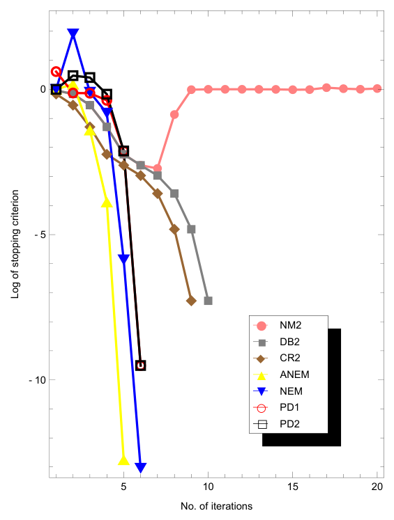
This section is devoted to examining the performance of the iterative methods discussed above for building both the MSR and its inverse. All computational tests were carried out in the Mathematica 14.0 computing environment [29], using the same hardware configuration in order to ensure a consistent and fair comparison. The numerical assessment includes several representative solvers, namely the Newton iteration (9), the Denman–Beavers iteration (10), the cyclic-reduction scheme (11), the Padé-based iterations (14) and (15), the proposed method (27), and its scaled version based on (45). In what follows, these methods are denoted respectively by NM2, DB2, CR2, PD1, PD2, NEM, and ANEM. To broaden the numerical comparison in response to recent developments in matrix-function algorithms, we also include an additional solver, denoted by SCH, as a Schur-based direct algorithm [1] for the principal MSR. Since SCH is a direct method, no iteration count is associated with it.

To measure the convergence behavior of the iterations, we employ the following relative error criterion in the $l_{\infty }$-norm:

$$E_{j+1}={\displaystyle \frac{\parallel U_{j+1}-U_j{\parallel }_{\infty }}{\parallel U_{j+1}{\parallel }_{\infty }}}\le ϵ,$$

(46)

where $ϵ$ is the prescribed tolerance. According to this stopping rule, the iterative process is terminated once two consecutive approximations become sufficiently close.

The example considered below should be viewed not as a single test problem, but as a benchmark family involving matrices of different sizes. More precisely, four test cases with distinct matrix dimensions are examined in order to provide a broader comparison under different computational settings.

Remark 2.

MSRs also appear in risk decomposition problems. Let $w\in {\mathbb{R}}^n$ be a vector of portfolio weights, and let $M\in {\mathbb{R}}^{n\times n}$ denote the corresponding covariance matrix. The total variance of the portfolio is expressed as

$${\sigma }^2=w^{\top }Mw={\parallel M^{1/2}w\parallel }^2,$$

where

$$M^{1/2}$$

is a symmetric MSR of M. The vector

$$M^{1/2}w,$$

can then be used to interpret the marginal contribution of each component to the overall portfolio risk. This idea is frequently employed in risk parity methods and factor-based risk decomposition. Therefore, efficient and accurate algorithms for computing MSRs are relevant in several applied fields, including control theory, financial mathematics, and systems engineering.

We also record the leading per-step floating-point cost of the fourth-order competitors used in the numerical comparison. For dense real $n\times n$ matrices, one matrix–matrix multiplication costs approximately $2n^3$ flops. Moreover, solving a dense matrix equation with n right-hand sides by LU factorization with partial pivoting costs

$${\displaystyle \frac{2}{3}}{n}^3+2n^3={\displaystyle \frac{8}{3}}{n}^3$$

flops, where the first term corresponds to the LU factorization and the second term to the two triangular solves. Therefore, inverse notation in formulas such as (27), (14), and (15) should be interpreted computationally as one dense linear solve, as discussed in Remark 1.

For the proposed method (27), the powers $U_j^2$ and $U_j^4$ can be formed using two matrix products, and the denominator factor

$$D_j=U_j\left(509I+994U_j^2+97U_j^4\right)$$

requires one additional matrix product. The update is then obtained by solving the right matrix equation

$$U_{j+1}{D}_j=103I+1006U_j^2+491U_j^4.$$

Thus, the leading cost of one NEM step is

$$3(2n^3)+{\displaystyle \frac{8}{3}}{n}^3={\displaystyle \frac{26}{3}}{n}^3\approx 8.67n^3,$$

flops. The same leading-order count is obtained for the Padé-type competitors PD1 and PD2, since they also require the construction of $U_j^2$, $U_j^4$, one additional product for the denominator or numerator factor, and one dense linear solve. The scaled version ANEM has the same leading rational-update cost, but it includes an additional scaling overhead due to the norm-balancing parameter in (45). This overhead is usually lower order if norm estimates are used, but it can be noticeable when full inverse-related quantities are computed (Table 1).

Table 1. Leading per-step dense flop counts for the fourth-order iterative competitors.

Method	Main Operations per Step	Leading Flop Count
PD1	3 matrix products + 1 dense linear solve	${\displaystyle \frac{26}{3}}{n}^3$
PD2	3 matrix products + 1 dense linear solve	${\displaystyle \frac{26}{3}}{n}^3$
NEM	3 matrix products + 1 dense linear solve	${\displaystyle \frac{26}{3}}{n}^3$
ANEM	NEM step + scaling overhead	${\displaystyle \frac{26}{3}}{n}^3+$ scaling overhead

For the largest dimension used in Example 1, namely $n=850$, the leading cost

$${\displaystyle \frac{26}{3}}{n}^3,$$

is approximately

$$5.32\times {10}^9,$$

flops per iteration for PD1, PD2, and NEM. Hence, for high-dimensional covariance matrices of the type discussed in Remark 2, reducing the number of iterations directly reduces the total leading arithmetic cost. This explains why the iteration count reported in the numerical tables is a meaningful indicator of computational efficiency, provided that all fourth-order rational methods are implemented through comparable dense linear solves rather than explicit matrix inverses.

Example 1.

Motivated by Remark 2, and in order to compare the behavior of different solvers in this setting [28], we take into account the following symmetric positive definite (SPD) matrix of size n and calculate its square root together with its inverse:

$$M={\left(n_{ij}\right)}_{n\times n}=\left\{\begin{array}{ccc}-1\hfill & & |i-j|=2,\hfill \\ -5\hfill & & |i-j|=1,\hfill \\ 12\hfill & & i=j.\hfill \end{array}\right.$$

For every tested dimension n, we numerically confirmed that ${\lambda }_{\min }(M)>0$; hence, M is SPD.

To obtain a reliable comparison among the competing iterative procedures, all numerical implementations were carried out under the same experimental conditions. In particular, each method was initialized with the identical starting matrix

$$U_0=M,$$

which is a standard admissible initialization for matrix sign-based and square-root-based iterations when M is nonsingular and $\sigma (M)\cap {\mathbb{R}}^{-}=\varnothing$. No solver was supplied with a problem-specific or preconditioned initial approximation.

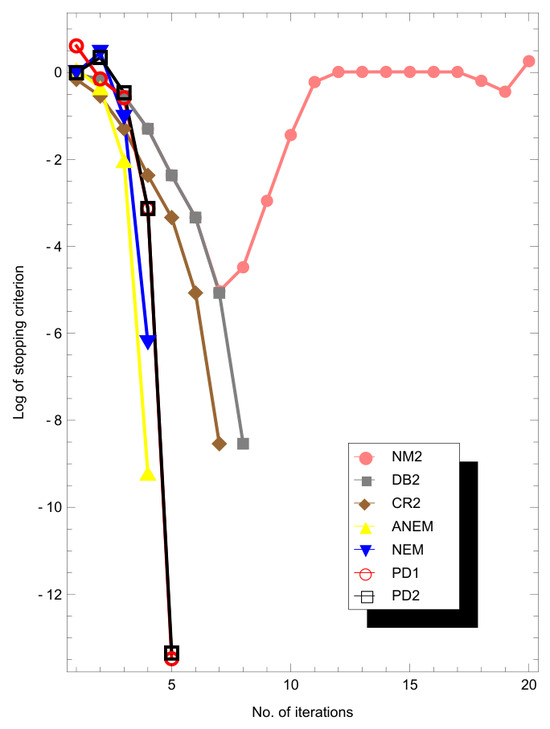
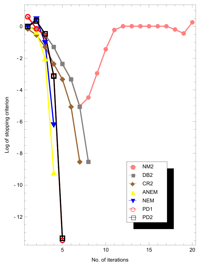
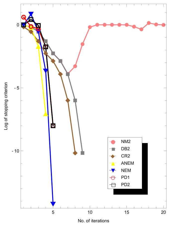
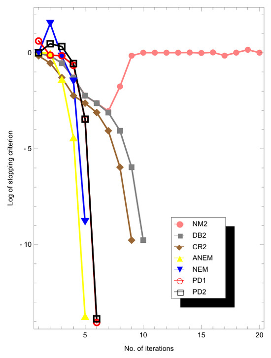
Furthermore, the same termination rule was used for all methods. The iterations were stopped as soon as the relative difference between two successive iterates satisfied (46) with the common tolerance $ϵ={10}^{-6}$ throughout all experiments, as stated in (46). This criterion is independent of the exact solution and is widely used in computations involving matrix functions. All algorithms were implemented in the same computational environment, relying on identical matrix arithmetic operations and the same norm evaluations. No solver-specific tuning, adaptive restarting, or problem-dependent optimization was employed. Thus, the reported iteration numbers reflect the intrinsic convergence behavior of the methods rather than differences in implementation. This unified experimental design ensures that the observed improvements of the proposed schemes are due to their higher-order convergence and favorable global behavior, rather than unequal initialization or stopping rules (Figure 3 and Figure 4).

Figure 3. Numerical outcomes for the MSR obtained in Experiment 1 with $n=150$.

Figure 4. Computational outcomes for the MSR obtained in Experiment 1 with $n=250$.

In Table 2, SCH denotes the Schur-based direct solver for the principal MSR. Since SCH is not an iterative method, it has no iteration count and is not governed by the stopping criterion (46). Therefore, for SCH we report the relative square root residual

$$R_{\mathrm{sq}}={\displaystyle \frac{\parallel U^2{-M\parallel }_{\infty }}{{\parallel M\parallel }_{\infty }}},$$

where U is the computed approximation to $M^{1/2}$. We also computed the inverse-consistency residual

$$R_{\mathrm{inv}}={\parallel UZ-I\parallel }_{\infty },$$

where Z denotes the corresponding approximation to $M^{-1/2}$. For the case $n=850$, the Schur-based computation gave

$$R_{\mathrm{inv}}=3.08\times {10}^{-12}.$$

The results show that SCH provides a highly accurate direct reference solver. At the same time, NEM remains competitive among the iterative methods and reaches a final stopping quantity of order ${10}^{-14}$. The accelerated version ANEM requires the smallest number of iterations among the tested iterative schemes. Moreover, unlike a direct Schur-based computation, the proposed sign-function framework naturally produces approximations to both $M^{1/2}$ and $M^{-1/2}$ through the block identity (35).

Table 2. Comparison of the iterative schemes and a Schur-based direct solver for Example 1 with $n=850$ and $ϵ={10}^{-6}$. For the iterative schemes, the last column reports the stopping quantity $E_{j+1}$ in (46); for the Schur-based direct solver, it reports the relative square root residual $R_{\mathrm{sq}}$.

Method	Iterations	Final Quantity
NM2	20	$1.07$
DB2	10	$5.27\times {10}^{-8}$
CR2	9	$5.27\times {10}^{-8}$
PD1	6	$3.10\times {10}^{-10}$
PD2	6	$3.11\times {10}^{-10}$
NEM	6	$9.03\times {10}^{-14}$
ANEM	5	$1.78\times {10}^{-13}$
SCH	–	$R_{\mathrm{sq}}=1.48\times {10}^{-13}$

The computational results obtained from this benchmark are compared with those produced by the Padé-based competitors, namely PD1 and its reciprocal version PD2, which have the same theoretical convergence order as the proposed method. In addition, Table 2 includes a Schur-based direct solver, denoted by SCH, for the largest tested dimension $n=850$. The results show that NEM is competitive among the fourth-order iterative schemes and reaches a smaller final stopping quantity than the Padé-based competitors in this experiment. The accelerated version ANEM reduces the number of iterations, while SCH provides an accurate direct reference solution. It should be noted that SCH is not an iterative sign-function method and therefore has no iteration count associated with (46). These observations confirm that the proposed method is effective among iterative sign-based and square-root-based solvers, while the Schur-based computation validates the accuracy of the obtained MSR.

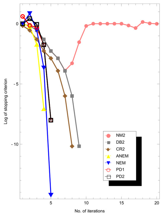
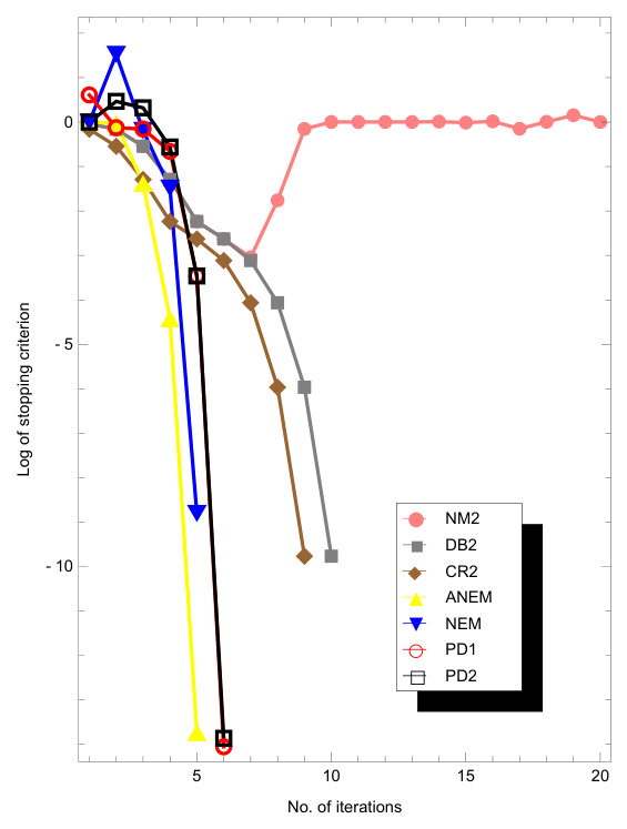
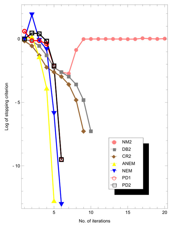
It is also important to note that NEM, despite having the same fourth-order convergence as PD1 and PD2, reaches convergence with fewer iterations in the reported tests. This directly reduces the total number of matrix–matrix products and the number of evaluations of the stopping criterion in (46). As a result, NEM is not only computationally efficient but also attractive for practical large-scale computations where the overall cost is a major concern (Figure 5 and Figure 6).

Figure 5. Numerical outcomes for the MSR obtained in Experiment 1 with $n=550$.

Figure 6. Numerical outcomes for the MSR obtained in Experiment 1 with $n=850$.

Example 2.

We consider three additional matrix classes with different spectral properties. The first test matrix is the regularized Hilbert matrix

$$M_1=H_n+{10}^{-2}I,{(H_n)}_{ij}={\displaystyle \frac{1}{i+j-1}},1\le i,j\le n,$$

which is a classical SPD test matrix. The second test matrix is the complex non-Hermitian matrix

$$M_2=(3+0.5\mathrm{i})I+0.2T+0.15\mathrm{i}K,$$

where

$$T=\left[\begin{array}{cccc}2& -1& & \\ -1& 2& -1& \\ & \ddots & \ddots & \ddots \\ & & -1& 2\end{array}\right],K=\left[\begin{array}{cccc}0& 1& & \\ -1& 0& 1& \\ & \ddots & \ddots & \ddots \\ & & -1& 0\end{array}\right].$$

The third test matrix is a nearly singular SPD matrix defined by

$$M_3=V{D}_{\eta }{V}^{\top },\eta ={10}^{-4},$$

where

$$D_{\eta }=\mathrm{diag}(\eta ,1,2,\dots ,n-1),$$

and $V={(v_{ij})}_{n\times n}$ is the discrete sine transform matrix

$$v_{ij}=\sqrt{{\displaystyle \frac{2}{n+1}}}\sin \left({\displaystyle \frac{ij\pi }{n+1}}\right),1\le i,j\le n.$$

The matrix $M_3$ is SPD and has a small eigenvalue equal to η, so it provides a controlled near-singular test.

For all three matrices in Example 2, we take $n=50$ and apply NEM and ANEM with the same tolerance $ϵ={10}^{-6}$. In addition to the stopping quantity $E_{j+1}$ in (46), we report the square root residual

$$R_{\mathrm{sq}}={\displaystyle \frac{\parallel U^2{-M\parallel }_{\infty }}{{\parallel M\parallel }_{\infty }}}$$

and the inverse-consistency residual

$$R_{\mathrm{inv}}={\parallel UZ-I\parallel }_{\infty }.$$

The numerical results are shown in Table 3.

Table 3. Performance of NEM and ANEM for the additional SPD, complex, and nearly singular matrices in Example 2 with $n=50$ and $ϵ={10}^{-6}$.

Matrix	Method	Iterations	${\mathit{E}}_{\mathit{j}+1}$	${\mathit{R}}_{\mathbf{sq}}$
$M_1$, SPD Hilbert-type	NEM	4	$1.58\times {10}^{-10}$	$2.81\times {10}^{-14}$
$M_1$, SPD Hilbert-type	ANEM	4	$1.74\times {10}^{-15}$	$2.71\times {10}^{-13}$
$M_2$, complex non-Hermitian	NEM	3	$1.20\times {10}^{-11}$	$1.09\times {10}^{-15}$
$M_2$, complex non-Hermitian	ANEM	3	$6.07\times {10}^{-16}$	$9.10\times {10}^{-16}$
$M_3$, nearly singular SPD	NEM	6	$6.73\times {10}^{-15}$	$9.83\times {10}^{-9}$
$M_3$, nearly singular SPD	ANEM	5	$5.87\times {10}^{-15}$	$6.85\times {10}^{-8}$

It should be emphasized that the stopping quantity $E_{j+1}$ and the square root residual $R_{\mathrm{sq}}$ measure different aspects of the computation. For well-conditioned matrices, these quantities usually decrease consistently. However, for nearly singular or highly ill-conditioned matrices, such as $M_3$, the difference between two consecutive iterates may reach the level of machine precision before the residual decreases to the same order. This explains why, for $M_3$, the value of $E_{j+1}$ is around ${10}^{-15}$, whereas $R_{\mathrm{sq}}$ remains around ${10}^{-8}$. The residual is still below the prescribed tolerance $ϵ={10}^{-6}$, but the gap indicates the expected sensitivity of the square root computation near singularity.

The inverse-consistency residuals corresponding to Table 3 are

Matrix	Method	Rinv
M1	NEM	1.00 × 10−14
M1	ANEM	7.53 × 10−15
M2	NEM	7.17 × 10−16
M2	ANEM	4.69 × 10−16
M3	NEM	6.15 × 10−13
M3	ANEM	8.62 × 10−13

• These results indicate that the proposed iteration remains effective for standard SPD matrices, complex non-Hermitian matrices whose spectra avoid the negative real axis, and nearly singular SPD matrices. The results for $M_3$ also show the expected sensitivity of the square root residual when the smallest eigenvalue is close to zero. Although the method satisfies the prescribed iteration-difference stopping criterion and $R_{\mathrm{sq}}$ remains below $ϵ={10}^{-6}$, the gap between $E_{j+1}$ and $R_{\mathrm{sq}}$ shows that, for nearly singular matrices, a residual-based check is useful in addition to the standard iteration-based stopping rule.

Example 3.

To further examine the effect of non-normality, we also test the proposed method on a Jordan-type matrix

$$M_4=4I+4J_n,n=50,$$

where $J_n$ is the nilpotent shift matrix

$$J_n=\left[\begin{array}{cccc}0& 1& & \\ & 0& 1& \\ & & \ddots & \ddots \\ & & & 0\end{array}\right].$$

The matrix $M_4$ has the single eigenvalue 4, but it is highly non-normal and defective. Hence, although its spectrum is safely contained in the positive real axis and the principal MSR is well defined, this example is useful for detecting possible transient growth in the early iterations of a rational matrix iteration.

Table 4 reports the iteration history of NEM and ANEM for Example 3. Here, ${\mathcal{U}}_j$ denotes the sign iteration applied to the block matrix in (35). The initial value satisfies

$$\parallel {\mathcal{U}}_0{\parallel }_{\infty }=8.$$

Thus, the column $\parallel {\mathcal{U}}_j{\parallel }_{\infty }$ is included to monitor whether the iteration produces a transient norm amplification.

Table 4. Iteration history of NEM and ANEM for the highly non-normal Jordan-type matrix $M_4=4I+4J_n$, $n=50$, in Example 3.

Method	Iteration	${\mathit{E}}_{\mathit{j}+1}$	${\mathit{R}}_{\mathbf{sq}}$	${\mathit{R}}_{\mathbf{inv}}$	$\parallel {\mathcal{U}}_{\mathit{j}+1}{\parallel }_{\mathit{\infty }}$
NEM	1	$1.44$	$1.20\times {10}^{-1}$	$3.45\times {10}^{-1}$	$4.11$
NEM	2	$5.70\times {10}^{-2}$	$7.08\times {10}^{-8}$	$7.49\times {10}^{-8}$	$3.98$
NEM	3	$2.62\times {10}^{-8}$	$7.58\times {10}^{-15}$	$2.36\times {10}^{-15}$	$3.98$
ANEM	1	$1.50$	$1.70\times {10}^{-1}$	$3.38\times {10}^{-1}$	$4.02$
ANEM	2	$7.67\times {10}^{-2}$	$6.70\times {10}^{-7}$	$6.99\times {10}^{-7}$	$3.98$
ANEM	3	$2.40\times {10}^{-7}$	$1.20\times {10}^{-14}$	$2.66\times {10}^{-15}$	$3.98$

The results in Table 4 show that both NEM and ANEM converge within three iterations for this defective non-normal matrix. Moreover, the norm of the sign iterate does not exhibit transient growth: starting from $\parallel {\mathcal{U}}_0{\parallel }_{\infty }=8$, it remains below $4.11$ throughout the computation.

5. Conclusions

The computation of the MSR and its inverse is important in both numerical analysis and applications, particularly for symmetric positive definite matrices where square roots and inverse square roots arise naturally. A classical example is the numerical treatment of second-order matrix differential equations, such as the model given in Equation (3). In this paper, we proposed and analyzed a fourth-order iterative method for the accurate and efficient computation of both the MSR and the inverse square root. The scheme was derived from a stable iteration for the matrix sign function. Its convergence properties were investigated, and the associated scaling strategy was discussed in detail. Numerical experiments, including comparisons with classical iterations, Padé-type schemes, recent sign-function-based competitors, and a Schur-based direct solver, were then presented to confirm the theoretical results and to demonstrate the robustness and computational competitiveness of the proposed approach. For applications requiring very high accuracy on ill-conditioned or nearly singular matrices, it is advisable to use a combined stopping rule that monitors both the iteration difference $E_{j+1}$ and the residual quantity $R_{\mathrm{sq}}$, rather than relying only on the difference between successive iterates. Based on the findings of this study, future work may consider extending the present iterative framework to other matrix functions, including matrix pth roots and the matrix exponential, while maintaining high-order convergence and numerical stability.

References

- Higham, N.J. Functions of Matrices: Theory and Computation; Society for Industrial and Applied Mathematics: Philadelphia, PA, USA, 2008. [Google Scholar]
- Salehi, S.; Lotfi, T. A globally convergent numerical method with fourth order for computing the matrix sign. Math. Methods Appl. Sci. 2025, 48, 7460–7468. [Google Scholar]
- Feng, Y.; Othman, A.Z. An accelerated iterative method to find the sign of a nonsingular matrix with quartical convergence. Iran. J. Sci. 2023, 47, 1359–1366. [Google Scholar] [CrossRef] [Scilit]
- Dehghani-Madiseh, M. On the solution of parameterized Sylvester matrix equations. J. Math. Model. 2022, 10, 535–553. [Google Scholar]
- Zaka Ullah, M.; Muaysh Alaslani, S.; Othman Mallawi, F.; Ahmad, F.; Shateyi, S.; Asma, M. A fast and efficient Newton-type iterative scheme to find the sign of a matrix. AIMS Math. 2023, 8, 19264–19274. [Google Scholar] [CrossRef] [Scilit]
- Dooren, P.V.; Bhattacharyya, S.P.; Chan, R.H.; Olshevsky, V.; Routray, A. (Eds.) Numerical Linear Algebra in Signals, Systems and Control; Lecture Notes in Electrical Engineering; Springer: Dordrecht, The Netherlands, 2011; Volume 80. [Google Scholar]
- Company, R.; Egorova, V.N.; Jódar, L.; Soleymani, F. A local radial basis function method for high–dimensional American option pricing problems. Math. Model. Anal. 2018, 23, 117–138. [Google Scholar]
- Kessy, A.; Lewin, A.; Strimmer, K. Optimal whitening and decorrelation. Am. Stat. 2018, 72, 309–314. [Google Scholar] [CrossRef] [Scilit]
- Nielsen, M.A.; Chuang, I.L. Quantum Computation and Quantum Information; Cambridge University Press: Cambridge, UK, 2010. [Google Scholar]
- Higham, N.J. Newton’s method for the matrix square root. Math. Comput. 1986, 46, 537–549. [Google Scholar] [CrossRef] [Scilit]
- Cross, G.W.; Lancaster, P. Square roots of complex matrices. Linear Multilinear Algebra 1974, 1, 289–293. [Google Scholar] [CrossRef] [Scilit]
- Soleymani, F.; Shateyi, S.; Haghani, F.K. A numerical method for computing the principal square root of a matrix. Abstr. Appl. Anal. 2014, 2014, 525087. [Google Scholar] [CrossRef] [Scilit]
- Soleymani, F.; Stanimirović, P.S.; Stojanović, I. A novel iterative method for polar decomposition and matrix sign function. Discret. Dyn. Nat. Soc. 2015, 2015, 649423. [Google Scholar] [CrossRef] [Scilit]
- Torkashvand, V. A two-step method adaptive with memory with eighth-order for solving nonlinear equations and its dynamic. Comput. Methods Differ. Equ. 2022, 10, 1007–1026. [Google Scholar]
- Khosravi Dehdezi, E.; Karimi, S. A fast and efficient Newton-Shultz-type iterative method for computing inverse and Moore-Penrose inverse of tensors. J. Math. Model. 2021, 9, 645–664. [Google Scholar]
- Traub, J.F. Iterative Methods for the Solution of Equations; Prentice-Hall: New York, NY, USA, 1964. [Google Scholar]
- Soleymani, F. Two novel classes of two-step optimal methods for all the zeros in an interval. Afr. Mat. 2014, 25, 307–321. [Google Scholar]
- Ivaz, K.; Asadpour Fazlallahi, M. Solving free boundary problem for an initial cell layer in multispecies biofilm formation by Newton-Raphson method. Comput. Methods Differ. Equ. 2021, 9, 899–907. [Google Scholar] [CrossRef] [Scilit]
- Soleymani, F.; Haghani, F.K.; Shateyi, S. Several numerical methods for computing unitary polar factor of a matrix. Adv. Differ. Equ. 2016, 2016, 4. [Google Scholar] [CrossRef] [Scilit]
- Denman, E.D.; Beavers, A.N. The matrix sign function and computations in systems. Appl. Math. Comput. 1976, 2, 63–94. [Google Scholar] [CrossRef] [Scilit]
- Meini, B. The Matrix Square Root from a New Functional Perspective: Theoretical Results and Computational Issues; Technical Report 1455; Dipartimento di Matematica, Università di Pisa: Pisa, Italy, 2003. [Google Scholar]
- Kenney, C.S.; Laub, A.J. Rational iterative methods for the matrix sign function. SIAM J. Matrix Anal. Appl. 1991, 12, 273–291. [Google Scholar] [CrossRef] [Scilit]
- Jung, D.; Chun, C. A general approach for improving the Padé iterations for the matrix sign function. J. Comput. Appl. Math. 2024, 436, 115348. [Google Scholar]
- Sharma, P.; Kansal, M. An iterative formulation to compute the matrix sign function and its application in evaluating the geometric mean of Hermitian positive definite matrices. Mediterr. J. Math. 2025, 22, 39. [Google Scholar] [CrossRef] [Scilit]
- Rani, L.; Kansal, M. Numerically stable iterative methods for computing matrix sign function. Math. Meth. Appl. Sci. 2023, 46, 8596–8617. [Google Scholar] [CrossRef] [Scilit]
- Getz, C.; Helmstedt, J. Graphics with Mathematica Fractals, Julia Sets, Patterns and Natural Forms; Elsevier: Amsterdam, The Netherlands, 2004. [Google Scholar]
- Sharma, P.; Kansal, M. Extraction of deflating subspaces using disk function of a matrix pencil via matrix sign function with application in generalized eigenvalue problem. J. Comput. Appl. Math. 2024, 442, 115730. [Google Scholar]
- Golzarpoor, J.; Ahmed, D.; Shateyi, S. Constructing a matrix mid-point iterative method for matrix square roots and applications. Mathematics 2022, 10, 2200. [Google Scholar] [CrossRef] [Scilit]
- Abell, M.L.; Braselton, J.P. Mathematica by Example, 5th ed.; Academic Press: Amsterdam, The Netherlands, 2017. [Google Scholar]
Disclaimer/Publisher’s Note: The statements, opinions and data contained in all publications are solely those of the individual author(s) and contributor(s) and not of MDPI and/or the editor(s). MDPI and/or the editor(s) disclaim responsibility for any injury to people or property resulting from any ideas, methods, instructions or products referred to in the content. |
© 2026 by the author. Licensee MDPI, Basel, Switzerland. This article is an open access article distributed under the terms and conditions of the Creative Commons Attribution (CC BY) license.