


Abstract
Neural metric learning is often assessed by retrieval accuracy, but a learned dissimilarity can rank examples well while failing to have norm-like algebraic structure. This paper studies a precise finite question: within a Euclidean-anchored residual family of neural dissimilarities, can one reduce sampled defects of homogeneity, subadditivity, and dyadic reconstruction on latent differences without destroying retrieval performance? The construction is inspired by asymptotically metrically normable (AMN) vector spaces, but its claims are finite, sampled, and latent: it does not prove global AMN rigidity or certify a metric on the input space. The framework is motivated by the observation that many learned similarities have the form and therefore encode an unbounded distance-like quantity or squared distance-like quantity behind a bounded affinity. The AMN-relevant object is this cost, not the bounded kernel value. We formalize bounded-perturbation stability of the large-scale specific energy , the conversion of subadditivity into multiplicative affinity consistency, and the quotient interpretation in which directions of zero large-scale cost are collapsed. The mathematical development then introduces finite dyadic diagnostics, learned-gauge and convex-unit-ball interpretations, finite norm-envelope witnesses, dyadic stability bounds, and refinement towers of witness norms. The empirical part reports full official Fashion-MNIST experiments with supervised-contrastive and proxy-anchor-style Euclidean baselines, post hoc audits for shrinkage, residual flexibility, off-training scales, and latent extrapolation, and a ten-seed full-query/full-gallery UCI Human Activity Recognition benchmark. The results show that Euclidean objectives can be stronger for Recall@1, whereas AMN-inspired residual regularization substantially reduces finite norm-like defects inside the residual family. The contribution is therefore a finite diagnostic and regularization framework for learned latent dissimilarities, not a state-of-the-art retrieval objective.
Keywords:
neural metric learning; neural dissimilarities; asymptotically metrically normable spaces; AMN-inspired regularization; geometric regularization; norm reconstruction; finite diagnostics; kernel-derived distances; quotient latent geometry; Fashion-MNIST; UCI HAR; sensor data MSC:
68T07; 46B20; 54E35; 68T09; 68T10
1. Introduction
Metric-learning algorithms are commonly judged by neighbor ranking, same-class retrieval, or embedding utility. Contrastive losses, triplet losses, and supervised contrastive objectives are effective for these tasks [1,2,3]. However, good retrieval performance does not by itself imply that the learned dissimilarity has the algebraic structure of a norm. Pairwise and triplet objectives constrain relative scores on sampled examples; they do not necessarily enforce homogeneity, subadditivity, or stable norm reconstruction [4,5]. A neural dissimilarity may therefore be useful for retrieval while still having scale defects or non-subadditive behavior.
This paper focuses on the following finite claim. Consider a residual neural dissimilarity evaluated on latent differences and already anchored to the Euclidean norm. We ask whether AMN-inspired finite penalties can make this dissimilarity more norm-like on sampled latent scales, while preserving most of its retrieval performance. The question is intentionally narrower than global metric certification. All diagnostics and guarantees in the paper concern finite samples of latent vectors and finite-scale sets; they do not prove that a trained network induces a metric or a norm on the original input space.
The motivation comes from Mu noz-García’s theory of asymptotically metrically normable (AMN) vector spaces [6]. In that theory, norm-like geometry is recovered from the large-scale behavior of a metric vector space. The present paper does not transfer AMN rigidity theorems to neural networks. Instead, it extracts an operational principle: if a learned dissimilarity is approximately homogeneous, approximately subadditive, and stable under a finite slope reconstruction, then it can be audited and regularized as a finite norm-like object.
A useful representation-learning example comes from exponential similarities. Suppose latent objects lie in a vector space E and a learned similarity has the form
for a Laplacian or exponential model, or for a Gaussian model. In the first case, is already distance-like; in the second case, the logarithm gives and the square root is the distance-like quantity. If, up to bounded local perturbations,
then
while the bounded directions are precisely . Thus, the effective large-scale geometry lives on the quotient : directions in are invariances, redundant coordinates, noise, or collapse, whereas the quotient carries the stable semantic norm. The finite framework developed below is a sampled analog of this quotient picture.
Let X be the input space, let be an encoder and write . The residual head is evaluated on differences and has the form
where is a scalar neural head, bounds the residual deformation and is a numerical stabilizer. The dissimilarity used in diagnostics is the symmetrized version
For a finite dyadic depth L, the associated slope estimator is
This estimator is a diagnostic, not a certified norm. It is chosen because dyadic scaling gives an explicit telescoping identity and a computationally simple finite analog of large-scale AMN slopes; off-grid audits later check whether the observed behavior is not restricted to the training scales.
The main contribution is a finite diagnostic and regularization framework for learned latent dissimilarities. Its theoretical component explains the diagnostics through dyadic slope stability, learned gauges, convexity of finite unit balls, finite norm-envelope witnesses, and refinement towers of witness norms. Its experimental component tests whether the resulting penalties reduce finite defects in a controlled residual family, while modern Euclidean metric-learning baselines provide retrieval context. The full-split Fashion-MNIST experiments show that supervised contrastive Euclidean embeddings can achieve higher Recall@1, whereas AMN-inspired terms reduce finite norm-like defects inside the residual family. UCI HAR provides a non-visual secondary check with the same qualitative residual-family signal.
The rest of the paper is organized as follows. Section 2 recalls the AMN motivation, kernel-energy interpretation, and related metric-learning work. Section 3 defines the residual dissimilarity, the finite diagnostics, the norm-envelope and refinement constructions, the training objective, and the experimental protocol. Section 4 reports Fashion-MNIST, UCI HAR, and supporting audits. Section 5 interprets the results, including the role of Euclidean anchoring and the limitations of the diagnostics. Section 6 summarizes the contribution and future directions.
2. Background and Related Work
2.1. AMN Vector Spaces and Finite Translation
Mu noz-García’s AMN theory studies metric vector spaces whose large-scale geometry is asymptotically normable [6]. For an exact norm N, the identities
encode scaling and subadditivity. AMN theory replaces such identities with asymptotic controls and reconstructs norm-like behavior from large-scale slopes such as
The present paper uses this theory as motivation, not as a direct theorem about trained neural networks. We work with finite latent differences and replace infinite large-scale limits by the finite dyadic estimator Equation (6). Table 1 separates the AMN ingredient, the finite neural counterpart, and the corresponding limitation. This separation is important: the rigorous statements below are finite stability, envelope, and refinement results; the AMN theory supplies the guiding norm-reconstruction viewpoint.
Table 1.
Translation from asymptotic AMN theory to the finite diagnostics used here. The table records which part is rigorous in the present finite model and what is not claimed.
2.2. Kernel-Derived Distances and Quotient Latent Geometry
Exponential similarities often hide an unbounded cost behind a bounded affinity. Applying AMN scaling directly to a bounded normalized RKHS distance,
would be uninformative when K is bounded, because all large-scale directions become bounded. The AMN-relevant object is instead the exponent. For a Laplacian or exponential form , one recovers the distance-like quantity . For a Gaussian form
is squared-distance-like and
is the corresponding distance-like quantity. If a learned distance-like quantity satisfies , then its AMN slope recovers and the directions invisible at large scale are . Thus, is the effective quotient latent space. This quotient interpretation is useful only under a stable large-scale model; it should not be applied to an arbitrary bounded kernel value.
The conversion back from a recovered norm-like distance to a positive-semidefinite kernel is a separate issue. Hilbertian or conditionally negative type assumptions can justify kernels such as or [7,8], but positive semidefiniteness is not automatic for a general norm-like distance. We therefore distinguish a stable distance-like energy from any downstream PSD kernel.
2.3. Specific Energy, Affinity Consistency and Information Viewpoint
The notation is also useful as a compact energy analogy. Here, E is a displacement cost, not a conserved physical energy. The stable quantity is the specific large-scale slope
when it exists. Bounded perturbations do not change this slope: gives the same asymptotic specific energy. In addition, if E is subadditive, then the exponential affinity is multiplicatively path-consistent:
This is the kernel-language counterpart of the subadditivity defect used later.
The entropy connection is only pointwise. A raw value is a logarithmic cost, not an entropy. After normalizing affinities into a neighborhood distribution
the quantity is a surprisal term and its expectation is a Shannon entropy [9,10]. Thus, the AMN-inspired diagnostics act on geometric cost, while entropy describes uncertainty of the induced neighbor distribution.
2.4. Scope of the AMN Connection
The AMN terminology is used in a restricted and operational sense. Translation invariance is built into the difference parametrization rather than learned as an input-space property. Vectors such as or are ambient latent-vector operations and may not be observed data differences. Small sampled defects imply controlled behavior on the sampled latent distribution and finite scales; they do not certify a global metric, a norm on the input space, or a finite necessary-and-sufficient AMN criterion.
2.5. Metric Learning and Geometry of Learned Dissimilarities
Classical metric learning includes large-margin nearest-neighbor learning [11], Siamese and contrastive approaches [1,12], triplet-based deep metric learning [3], and supervised contrastive learning [2]. More recent pair-weighting and proxy-based objectives, including Circle Loss and Proxy Anchor, improve optimization and retrieval behavior [13,14]; surveys emphasize loss design, sampling, and evaluation protocol [4,5,15,16,17]. These objectives optimize task relations among samples, but they do not necessarily enforce homogeneity, subadditivity, or norm reconstruction for a learned dissimilarity.
The baselines answer two questions. Euclidean triplet, supervised-contrastive, and proxy-anchor-style baselines contextualize retrieval performance; they are norm-like by construction and are not expected to have large finite defects. The residual task-only model is the main geometric comparator, because it has the same residual capacity without AMN-inspired penalties. The non-AMN controls test whether the effect is generic regularization. The experiments should therefore be read as a controlled study of finite geometric regularization, complemented by standard retrieval baselines, rather than as a claim of state-of-the-art retrieval accuracy.
3. Materials and Methods
All computational experiments and analyses were run with Python 3.12.11. The principal software packages were PyTorch 2.7.1+cu118, NumPy 2.0.2, pandas 2.3.2, scikit-learn 1.6.1, and Matplotlib 3.10.6. No laboratory instruments, reagents, or commercial measurement agents were used.
3.1. Latent Residual Dissimilarity
Let denote an input-label pair, where is an observation and is its class label. The observation may be an image or a tabular feature vector. The encoder maps inputs to latent vectors , and all learned dissimilarities are evaluated on latent differences . The residual function is defined in Equation (4). In the final experiments, , and . Since and , the multiplicative factor in Equation (4) lies between and , so the Euclidean factor prevents negative values and anchors the model to a norm-like reference. In particular, apart from the small stabilizer, the residual family is bi-bounded by the Euclidean norm: . For the final value , this is the interval . Therefore, the experiment asks whether finite AMN-inspired penalties reduce residual geometric defects inside this Euclidean-anchored family, not whether they discover normability from an arbitrary dissimilarity.
The raw residual head need not be even in v. For this reason, the function used for retrieval, training diagnostics, and AMN-inspired losses is the symmetrized dissimilarity defined in Equation (5). By construction, . Strictly speaking, because of the stabilizer and because triangle inequalities are only regularized empirically, is used as a non-negative symmetric dissimilarity rather than as a certified metric. The additive stabilizer is retained in numerical denominators to avoid division by values close to zero.
Remark 1 (Latent-vector nature of the regularizer).
The finite AMN-inspired terms are applied after encoding, not in the raw input space. Translation invariance is therefore imposed by the difference parametrization . The vectors and used in the losses are latent-vector operations and need not be observed pair differences. The regularizer should therefore be interpreted as controlling the ambient latent extension of the learned dissimilarity on sampled scales.
Figure 1 summarizes the latent-difference workflow, and Table 2 lists the main objects used in the definitions and diagnostics.
Figure 1.
Pipeline. Inputs are encoded into latent vectors. The residual dissimilarity is evaluated on differences , and finite AMN-inspired diagnostics measure homogeneity, subadditivity, and reconstruction defects on sampled latent-vector operations.
Table 2.
Main notation. The table separates trained objects from derived diagnostics and records the status of each quantity.
3.2. Finite AMN-Inspired Defects
All finite diagnostic quantities are computed from minibatch samples of latent differences. Let denote the empirical distribution that samples latent pair differences from the vectors in minibatch B. The implementation samples the two indices independently with replacement, so exact self-pairs may occur with probability ; the numerical stabilizer in the denominators prevents division by zero in those rare cases. When several variables are written under an expectation, they are sampled independently unless stated otherwise. Let be the set of scaling factors used in the trained losses and primary reported diagnostics, let be a numerical stabilizer, and let . For a non-negative even dissimilarity on latent differences, define the finite dyadic estimator by Equation (6), replacing by when necessary. In the experiments, for diagnostics and for the principal Fashion-MNIST runs.
The homogeneity defect measures whether scaling v by scales the value by :
The subadditivity defect measures normalized violations of the triangle inequality in latent-difference form:
The reconstruction defect compares the learned dissimilarity with its finite dyadic estimator:
The reported diagnostics use the absolute normalized quantities in Equations (15)–(17). The differentiable training losses use the corresponding squared normalized quantities, as defined in Definition 2.
The dyadic estimator is used because repeated doubling gives a telescoping identity in Proposition 1, is cheap to evaluate during training, and matches the large-scale-slope intuition behind AMN reconstruction. The choice is not unique. Other finite-scale grids could be used; this is why the experiments include off-training-scale audits at non-dyadic and intermediate factors. The finite results below therefore justify the estimator on its chosen scale set rather than proving the uniqueness of dyadic scaling. Table 3 summarizes the reporting and regularization roles of the three defects.
Table 3.
Roles of the finite diagnostic quantities. The same quantities are used for reporting and, in squared form, for regularization, but none of them is by itself a global normability certificate.
3.3. Finite-Stability Statement
The following proposition is the finite mathematical bridge between AMN intuition and the implemented estimator. It is a stability statement for Equation (6), not a characterization of asymptotic AMN normability. The statement is written for a symmetrized dissimilarity, which matches Equation (5).
Proposition 1 (Finite stability of dyadic AMN-inspired reconstruction).
Let be a non-negative function and let . Define
Then:
- (i)
- The dyadic homogeneity boundary identity isThus, if normalized slopes vary little over the observed dyadic range, is approximately homogeneous.
- (ii)
- If, for every ,then
- (iii)
- The reconstruction error satisfies
The proof is given in Appendix A. The proposition formalizes the diagnostic intuition: homogeneity controls variation of normalized slopes, subadditivity controls finite triangle behavior, and both improve the stability of the reconstructed estimator. Its practical significance is finite consistency. It gives a reason for monitoring and regularizing the three defects together; it does not prove that small empirical losses certify a global norm or metric.
The next statement makes the link between dyadic homogeneity and reconstruction error more explicit. It is stated along one ray and uses log-slopes to avoid asymmetric ratio bounds.
Proposition 2 (Relative dyadic slope control).
Let and suppose that for . If there is such that
then, for every ,
and the relative reconstruction error satisfies
For small η, the right-hand side is . Thus, finite dyadic homogeneity gives a quantitative finite control of the dyadic reconstruction error along the same ray.
A second geometric interpretation is useful because the residual family has the multiplicative form , up to the small stabilizer. This places the model in the language of gauges and unit balls.
Proposition 3 (Gauge interpretation of the residual family).
Let be even and homogeneous of degree zero, and define for and . Then ρ is even and homogeneous of degree one. If, in addition, q is bounded above and below away from zero, the unit set
is compact, absorbing, and centrally symmetric. Under these assumptions, ρ is a norm if and only if is convex, equivalently if and only if ρ is subadditive.
This proposition explains the roles of the finite penalties. The homogeneity term encourages the residual factor to be stable along rays; the symmetrization enforces central symmetry; the subadditivity term is a sampled convexity test for the induced unit ball; and the reconstruction term checks whether the finite dyadic slope average is stable. The proposition also clarifies why the Euclidean anchor narrows the claim: the learned object is a bounded deformation of a known norm, not an arbitrary dissimilarity.
3.4. Finite Norm-Envelope Certificate
The gauge interpretation can be made constructive on a finite latent sample. Let be a finite centrally symmetric set of nonzero latent differences and let . For an even positive function , define the finite normalized atom set and its convex hull by
The Minkowski functional of this finite unit ball is
Equivalently,
Thus is the finite sublinear envelope generated by the sampled values of . It is computable by linear programming after fixing the atom set S.
Theorem 1 (Finite norm-envelope certificate).
Let be finite, centrally symmetric and spanning , and let be even. Then is a compact, centrally symmetric convex body in , and its Minkowski functional is a norm on . Moreover:
- (i)
- for every .
- (ii)
- is the largest seminorm on whose restriction to S is bounded above by ρ. In other words, if p is any seminorm with for all , then for all .
- (iii)
- Define the finite-envelope gapThen
- (iv)
- If, for some , every decomposition with and real coefficients satisfiesthen .
This theorem turns the sampled subadditivity question into a finite certificate: if the finite-envelope gap is small, the learned dissimilarity admits an explicit norm that approximates it on the sampled latent differences. The gap is one-sided because is constructed as the largest norm lying below the observed values on S. A large gap indicates that the sampled unit ball contains nonconvex or non-norm-like radial features that are removed by convexification.
The finite dyadic estimator can now be related not only to the learned dissimilarity but also to the norm envelope.
Corollary 1 (Dyadic reconstruction relative to the finite envelope).
Let the assumptions of Theorem 1 hold and let . Suppose that the normalized dyadic slopes are positive and satisfy Equation (23) for , where the values are defined on the ambient latent space. Then
Thus, dyadic homogeneity controls the reconstruction of along sampled rays, while the envelope gap controls how far is from an explicit finite norm on the sampled difference set. The bound is intentionally finite: it concerns the chosen sample S, the chosen dyadic range, and the ambient values of at the scaled points.
The same finite construction also gives a clean asymptotic interpretation when one considers a sequence of increasingly rich finite certificates.
Theorem 2 (Asymptotic limit of finite certificates).
Let E be a finite-dimensional real vector space. For each n, let be finite, centrally symmetric and spanning, and let be the norm generated by Equation (28) from values . Assume that there are constants such that
for all n. Then there is a subsequence such that converges locally uniformly on E to a norm p. Along any such convergent subsequence, if , then for every sequence contained in a fixed compact subset and with ,
This theorem is not used as an empirical claim about a single neural network. Its role is conceptual: it explains how a sequence of finite certificates with vanishing envelope gaps can converge to an actual norm, thereby connecting the finite procedure back to the AMN intuition without asserting global normability from one finite experiment.
3.5. Refinement Towers and Finite AMN Limits
The envelope construction also allows a closer finite analog of AMN norm reconstruction. In the asymptotic AMN picture, a norm emerges as a limit of rescaled metric information. In the neural finite setting, the corresponding object is not a single limit in scale only, but a sequence of refined finite certificates: more latent differences, more probed scales, deeper dyadic averages, or improved residual heads produce a succession of witness norms.
Definition 1 (Finite AMN-refinement tower).
Fix a finite-dimensional real vector space E. A finite AMN-refinement tower is a sequence
where is finite, centrally symmetric and spanning, is even, is the norm-envelope witness defined by Equation (28), and is the finite-envelope gap. The tower is uniformly anchored if there exists such that
for all n. For a compact set , define the refinement gap
The following theorem records the monotone situation in which the dissimilarity is fixed, and only the sampled latent directions are refined. This is the cleanest finite analog of adding more observed directions to an approximate unit ball.
Theorem 3 (Monotone refinement for a fixed dissimilarity).
Let be finite, centrally symmetric, and spanning, and let ρ be an even positive function on . Define
and
Assume that is a compact convex body in E. Then , the gauges satisfy
converges to in Hausdorff distance, and converges locally uniformly to the norm . If, in addition, , then for every sequence contained in a fixed compact subset and satisfying ,
For trained neural models, the dissimilarity may also change between refinement levels. In that case, exact monotonicity is replaced by a Cauchy condition on the witness norms.
Theorem 4 (Coherent finite AMN-refinement limit).
Let be a uniformly anchored finite AMN-refinement tower in a fixed finite-dimensional space E. Suppose that for every compact set ,
Then converges locally uniformly to a norm on E. For with , define the relative dyadic reconstruction residual
where is computed from . If remains in a fixed compact set, , and
then
The tower formulation identifies the finite analog of the AMN limiting picture used in this paper. The asymptotic AMN construction reconstructs a norm from the large-scale behavior of one metric; here, a norm-like latent geometry is obtained as the local uniform limit of finite witness norms, provided the sampled envelopes are coherent across refinements. The theorem is conditional: it does not assert that training automatically produces such a tower. It states what additional coherence would be needed to interpret successive finite audits as convergence toward a limiting norm.
Remark 2 (Collapsed directions and quotient geometry).
If the lower bound in Equation (37) is dropped, a locally uniform limit of the witness norms may be a seminorm. Its null space
then defines a quotient norm on . This is a natural finite counterpart of the AMN intuition that bounded or collapsed directions can be factored out before a norm-like geometry is recovered. In representation-learning terms, corresponds to latent directions that the learned dissimilarity does not separate at the limiting resolution of the tower.
3.6. Stable Kernel-Derived Distance Quotient Model
The quotient interpretation in Section 2.2 can be stated as a simple model result. It is not a neural training theorem; rather, it records the AMN large-scale mechanism behind exponential similarities whose logarithmic, or square-root logarithmic, transform is a bounded perturbation of a linear seminorm.
Proposition 4 (Stable kernel-derived distance and quotient latent geometry).
Let E be a finite-dimensional real vector space, let H be a normed vector space, let be linear, and let be a symmetric distance-like quantity satisfying, for some ,
Define the large-scale slope and bounded-direction set by
Then the limit exists for every and
Consequently, ν induces a norm on the quotient by .
The proof is immediate and is included in Appendix A. If a learned exponential similarity has Laplacian form and the logarithmic quantity satisfies Equation (48), then AMN scaling recovers the stable quotient distance . For Gaussian similarities, the same statement applies to the square-root log-distance in Equation (11), while itself should be read as a squared distance-like quantity. The directions in are precisely those that the kernel-derived distance cannot distinguish at a large scale. The statement does not assert that an arbitrary learned kernel yields a metric: symmetry, separation, and triangle-type properties must still be checked or regularized. This proposition is the clean model case that the finite norm-envelope and refinement-tower diagnostics approximate on sampled latent differences.
Corollary 2 (Specific-energy stability and affinity consistency).
Let be two distance-like quantities satisfying for all and some . If
exists, then exists and equals . In addition, if D is subadditive on triples,
then the exponential affinity satisfies
This corollary gives the precise sense in which the energy language is useful here. Bounded perturbations conserve the AMN-specific energy, while subadditivity of the distance-like energy becomes multiplicative consistency of the corresponding bounded affinity. The statement is not a physical conservation law and does not make an entropy. Entropic quantities enter only after normalization of affinities into probabilities, as described in Section 2.3.
Finally, the dyadic grid used in training does not by itself control all intermediate scales. The following conditional statement records the additional regularity needed to transfer dyadic control to off-grid scales.
Lemma 1 (Intermediate-scale control under log-scale regularity).
Fix and define on an interval . Let be a grid such that every is within distance at most of some grid point. If is M-Lipschitz on I and
then every satisfies
The lemma is not used as a training guarantee because the Lipschitz constant of the trained neural head is not certified in the experiments. Its purpose is to identify the missing regularity assumption behind off-dyadic generalization and to motivate the supplementary unseen-scale audits.
Corollary 3 (From expected losses to sampled finite defects).
Let
If the squared training losses satisfy , and under the sampling distributions used in training, then
and, for any ,
In particular, with probability at least over a sampled pair ,
The corollary is intentionally elementary: it uses Jensen’s inequality and Markov’s inequality. Its purpose is to close the gap between the pointwise assumptions of Proposition 1 and the minibatch expected losses optimized by the algorithm. It does not turn the empirical regularizer into a global metric certificate.
Corollary 4 (Empirical concentration for reported finite defects).
Fix a trained model and one diagnostic distribution, for instance, the training-gallery or test-query latent-difference distribution. Let be independent draws of one of the non-negative normalized defects H, S or R in Equations (56)–(58). If almost surely and , then Hoeffding’s inequality [18] gives, for every ,
Consequently, the diagnostic estimates reported from sampled differences should be interpreted as finite-sample estimates of the corresponding sampled-distribution defects, conditional on the trained model and the chosen latent distribution.
This concentration statement is also deliberately modest and follows from Hoeffding’s inequality [18]. It addresses Monte Carlo error in reporting finite defects after a model has been trained, while learning-theoretic generalization of the neural encoder and held-out validation remain separate issues.
3.7. Mathematical Contribution and Limitations
The primary contribution is a finite framework for diagnosing and regularizing norm-like geometry in learned latent dissimilarities. It has three parts. First, the diagnostics , , and measure finite violations of scaling, subadditivity, and dyadic reconstruction on sampled latent differences. Second, the theoretical statements explain what those diagnostics control in the finite setting: stability of the dyadic estimator, a gauge and unit-ball interpretation, finite norm-envelope witnesses, refinement limits under explicit coherence assumptions, and quotient behavior for stable kernel-derived distances. Third, the experiments test whether adding the corresponding penalties improves finite geometry inside a Euclidean-anchored residual family.
The limitations are equally important. The results do not prove AMN rigidity, global normability, convergence of as , or a metric certificate on the original input space X. They also do not show that the residual family is a better retrieval model than Euclidean supervised-contrastive or proxy-based objectives. The full-split experiments deliberately include those Euclidean baselines to show that the proposed framework is about finite geometric control and auditability, not retrieval leadership.
The hyperparameter protocol should be read in this light. The AMN weights were selected in exploratory runs and then kept fixed for the final controlled audits. No additional validation split was introduced beyond the held-out evaluation subsets and official test sets. Therefore, the reported numerical results are best interpreted as a reproducible finite-geometry audit with fixed choices rather than as an optimized model-selection claim. The post hoc shrinkage, residual-scale, and off-grid audits were added to test alternative explanations and were not used to tune the main reported models.
3.8. Synthetic Diagnostic Example
Before using neural networks, it is useful to inspect the diagnostics on explicit functions. We evaluate six functions in : the Euclidean norm, an anisotropic norm with positive diagonal A, a superlinear radial perturbation , a bounded log-periodic radial perturbation, a homogeneous but nonconvex gauge on the first two coordinates, and a dyadic-aliasing perturbation away from the origin. For any exact norm, for all k, so and the three finite diagnostics vanish up to numerical precision. The homogeneous nonconvex gauge shows why homogeneity and reconstruction are not enough without subadditivity. The dyadic-aliasing perturbation shows why off-grid scale audits are informative: it can look stable on dyadic scales while varying at intermediate scales.
Table 4, Table 5 and Table 6 and Figure 2 illustrate the finite mechanism behind Propositions 1–3 and Theorems 1 and 3. Exact norms are reconstructed exactly by the finite dyadic estimator. The quadratic perturbation has rapidly changing normalized slopes and a large reconstruction defect. The homogeneous nonconvex gauge has negligible homogeneity and reconstruction defects but a nonzero subadditivity defect and a positive finite-envelope gap, showing why sampled convexity is necessary. The dyadic-aliasing perturbation has nearly zero dyadic homogeneity, reconstruction, and envelope defects on sampled dyadic directions but a visible off-grid homogeneity defect, motivating the unseen-scale diagnostics described in the supplementary scripts. The refinement demonstration shows the other direction of the theory: for an exact norm, finite sampled atom hulls give polygonal witness norms that converge as directions are refined. Thus, the synthetic examples support the interpretation of , , and as complementary finite diagnostics of norm-like behavior rather than as arbitrary regularization terms.
Table 4.
Synthetic finite diagnostics in . Values are Monte Carlo averages over 20,000 Gaussian pairs, with . The dyadic homogeneity column uses the training scales ; the off-grid column uses .
Table 5.
Finite norm-envelope diagnostic on 96 directions in . The envelope gap is zero for sampled directions of exact norms, positive for a homogeneous nonconvex gauge, and does not detect the dyadic-aliasing radial perturbation unless off-grid scales are evaluated.
Table 6.
Finite norm-refinement tower demonstration in . Increasing the number of sampled directions refines the convex atom hull and decreases the witness-gauge overestimate on a dense probe grid. The refinement gap is the maximum change relative to the previous level.
Figure 2.
Synthetic normalized dyadic slopes for representative explicit functions. Exact norms have constant normalized slopes. Scale-dependent perturbations produce finite-scale slope variation; the dyadic-aliasing perturbation illustrates that dyadic scales alone may miss intermediate-scale oscillations.
3.9. Training Objective and Variants
Definition 2 (Training objective and finite AMN-inspired regularizer).
Let be the empirical distribution of anchor-positive-negative triples , where is an anchor observation, has the same class label as , and has a different class label. Let , and . For margin , define the task loss by
Let be independent minibatch latent differences and let be independent of them. With this convention, the squared AMN-inspired loss terms are
The optional symmetry and non-degeneracy terms are
where and are lower and upper slope bounds. For non-negative weights , , , and , define the total training objective by
In all final reported experiments, , , , , and . The two Fashion-MNIST AMN-inspired variants differ in the three main weights:
- AMN-inspired balanced: , , ;
- AMN-inspired geom-first: , , .
We compare them against a Euclidean triplet baseline, a residual task-only dissimilarity with , and non-AMN controls: stronger weight decay, a generic smoothness penalty, reconstruction-only regularization, and homogeneity plus subadditivity without the explicit reconstruction term. The UCI HAR corroboration uses the same objective, but only the Euclidean, residual task-only, and AMN-inspired balanced families are compared; because it is a small CPU secondary run rather than the Fashion-MNIST controlled experiment, the AMN weights are set to , , and .
The Euclidean triplet baseline is included as a standard norm-constrained reference, and the residual task-only model is the main within-family comparator. We also executed a full official Fashion-MNIST split audit with supervised-contrastive and proxy-anchor-style Euclidean baselines. These objectives change the training criterion and are therefore not direct tests of the AMN-inspired penalties, but they give an explicit reference for retrieval performance under modern norm-like embeddings.
Hyperparameter Selection
The AMN weights were selected in an exploratory Fashion-MNIST grid and then fixed before the final ten-seed controlled run, the non-AMN control run, and the full official split audit. The exploratory range was , and on a reduced candidate sweep. Selection used a scalar score that favored defect reductions while penalizing Recall@1 loss relative to the residual task-only run. No separate validation split was introduced beyond the held-out evaluation subset; therefore, these weights are reported as pre-fixed exploratory choices rather than as statistically optimized hyperparameters, and the full official split should be read as a fixed-weight audit rather than as a validation-selected benchmark. Appendix B provides the compact hyperparameter and experimental-protocol details underlying these settings; Table A2 reports a representative sensitivity excerpt from the archived grid.
3.10. Data Sets, Implementation and Evaluation Protocol
3.10.1. Primary Benchmark: Fashion-MNIST
The main experiments use Fashion-MNIST [19], a public benchmark of Zalando article images. The dataset contains 70,000 grayscale images of size : 60,000 training images and 10,000 test images. Each image belongs to one of ten classes: T-shirt/top, trousers, pullover, dress, coat, sandal, shirt, sneaker, bag, and ankle boot. Figure 3 shows representative images from the public Fashion-MNIST visualization. The benchmark was chosen because it keeps the simple size and split structure of MNIST [20] but replaces handwritten digits with visually more heterogeneous product images, making it a controlled yet nontrivial test bed for retrieval and metric-learning behavior.
Figure 3.
Representative Fashion-MNIST images from the public project visualization. The classes include clothing items and accessories such as tops, trousers, shoes, bags, and ankle boots. Source: Fashion-MNIST project repository, MIT license.
For computational control and paired multi-seed auditing, the controlled Fashion-MNIST experiments use ten random seeds, stratified training subsets of 20,000 examples and test subsets of 5000 examples. Retrieval evaluation uses up to 3500 test queries against a 16,000-example training gallery. These limits were chosen to make the residual variants, non-AMN controls, robustness probes, and paired statistics comparable under a fixed compute budget. To address full-split reproducibility and modern-baseline context, we additionally ran the complete official 60,000/10,000 split over ten seeds for Euclidean triplet, supervised contrastive, proxy-anchor-style, residual task-only, AMN-balanced, and AMN-geometry-first variants. In this full-split audit, all 10,000 test examples are queries and the 60,000 training examples form the gallery; reconstructed-distance retrieval is skipped for tractability, but the finite reconstruction defect is still computed. The encoder is a compact convolutional neural network producing a latent embedding of dimension 32. Training and evaluation were implemented in PyTorch 2.7.1+cu118 [21].
3.10.2. Secondary Non-Visual Benchmark: UCI HAR
The main cross-domain corroboration uses the UCI Human Activity Recognition Using Smartphones dataset (UCI HAR) [22,23]. The data consist of smartphone accelerometer and gyroscope measurements collected from 30 volunteers performing six activities: walking, walking upstairs, walking downstairs, sitting, standing, and laying. The public benchmark provides an official subject-based split of 7352 training records and 2947 test records, and represents each window by a 561-dimensional feature vector derived from s inertial-sensor windows sampled at 50 Hz with overlap. This benchmark is non-visual: the inputs are not pixels but standardized sensor-derived feature vectors. It was chosen because it keeps the supervised retrieval setting and class-label structure while testing the AMN-inspired mechanism on tabular time-series-derived data rather than images.
In the UCI HAR run, the official 561-feature vectors are standardized using the training-set mean and standard deviation. The encoder is a compact multilayer perceptron with hidden dimension 64 and latent dimension 32. The official train/test split is fixed; the reported seeds affect initialization and minibatch sampling, not the subject split. The non-visual corroboration uses ten seeds and the full official evaluation geometry: all 2947 test records are queries and all 7352 training records form the gallery. Reconstructed-distance retrieval is skipped, and only the diagnostic reconstruction defect is reported. The UCI HAR experiment remains secondary because it uses a compact CPU protocol and no separate hyperparameter search. Figure 4 gives a two-dimensional PCA visualization of the standardized sensor features.
Figure 4.
PCA visualization of representative UCI HAR records after standardizing the 561-dimensional sensor-feature vectors. The plot is not used for training; it illustrates that the non-visual benchmark has class structure in tabular inertial-sensor features. Source: UCI HAR public dataset.
3.10.3. Auxiliary Image-Domain Check: Scikit-Learn Digits
We retain a smaller auxiliary experiment on the handwritten Digits dataset distributed with scikit-learn. This dataset contains 1797 images of handwritten digits, each represented as an grayscale image with integer pixel values in the range 0–16, and has ten classes corresponding to the digits 0–9 [24]. Representative examples are shown in Figure 5. Digits is no longer the main secondary benchmark, because it is still an image dataset; it is kept only as a small image-domain mechanism check.
Figure 5.
Representative examples from the scikit-learn Digits dataset. The images are handwritten-digit thumbnails; the displayed examples use the first available sample from each class after loading the dataset.
For the Digits pilot, the images are rescaled to , upsampled by nearest-neighbor replication to , and padded to so that the same convolutional code path can be reused. The supplementary scripts generate deterministic stratified train/test splits with a default test fraction of . The archived pilot summaries use the same residual family and finite diagnostics as the Fashion-MNIST study, but they are interpreted only as an auxiliary check of the mechanism.
3.10.4. Evaluation and Statistical Protocol
Retrieval metrics are computed using each test example as a query and ranking training-gallery examples by increasing learned dissimilarity. Hence, the query itself is not present in the gallery. For , Recall@k is defined as
where Q is the query set and is the class label of query q. In particular, Recall@1 is nearest-neighbor retrieval accuracy under this label criterion. We also report nearest-neighbor accuracy and mean average precision where applicable. Geometry is evaluated by , , , the dyadic homogeneity defects at 2 and 4, and the magnitude and rate of triangle violations.
Unless explicitly stated otherwise, reported values are means and standard deviations over seeds. Fashion-MNIST paired comparisons are computed by pairing variants with the residual task-only baseline at the same seed. We report descriptive paired differences, paired t-tests, and Wilcoxon signed-rank tests in the Supplementary Material (CSV files); the main text uses these values only to indicate seed-level consistency of the defect reductions. The full official split audit uses ten seeds for all six variants. The additional Fashion-MNIST theory audits use three seeds and are reported as targeted diagnostics rather than as new model-selection sweeps. UCI HAR uses ten seeds on the fixed official subject split and is interpreted as secondary corroboration, not as a broad non-visual benchmark claim. Robustness probes for the image benchmark are included for Gaussian noise, central occlusion, contrast perturbation, and pixel shift; they are secondary diagnostics and are not used to claim universal robustness. Table 7 summarizes the main training, evaluation, and reproducibility protocol.
Table 7.
Training, evaluation and reproducibility protocol. The table lists the details most relevant for auditing the reported experiments.
4. Results
The empirical analysis is organized around the geometric claim rather than around a state-of-the-art retrieval claim. The key comparison is within the same residual family: task-only versus AMN-inspired variants. Euclidean triplet learning is reported as a standard norm-like reference, and the control regularizers test whether the observed changes are due merely to additional regularization.
4.1. Fashion-MNIST Controlled Experiment
Table 8 reports the controlled Fashion-MNIST results. All entries are means and standard deviations over ten paired seeds. The Euclidean triplet baseline is nearly defect-free because it is a norm in the learned embedding. The residual task-only model gives the highest Recall@1 among the residual models, but it has large finite homogeneity and reconstruction defects. AMN-inspired balanced changes Recall@1 from to while reducing from to , from to , and from to . AMN-inspired geom-first further reduces the defects at a slightly larger retrieval cost.
Table 8.
Fashion-MNIST controlled experiment. Values are the mean ± standard deviation over ten seeds. The Euclidean triplet baseline is a standard triplet-trained embedding with Euclidean latent distance.
Table 9 reports paired differences relative to the residual task-only baseline with descriptive 95% confidence intervals. The supplementary CSV files also include paired t-tests and Wilcoxon signed-rank tests; all p-values are uncorrected and are used only to show seed-level consistency of the defect reductions, not to claim broad distribution-free superiority across data sets. For both AMN-inspired variants, the reductions in all three finite defects are consistent across the ten seeds. The Euclidean triplet line is included only as a rigid reference.
Table 9.
Paired Fashion-MNIST differences relative to residual task-only. Entries are mean paired differences with descriptive 95% confidence intervals. Negative defect differences indicate lower finite defects.
Figure 6 displays the per-seed finite defects. The plots show that the reported defect reductions are not driven by a single anomalous seed: both AMN-inspired variants are below the residual task-only curve for , , and throughout the paired run.
Figure 6.
Per-seed Fashion-MNIST finite defects. Each point corresponds to one seed. AMN-inspired variants consistently reduce the three diagnostics relative to the residual task-only baseline.
Figure 7 and Figure 8 provide visual summaries of the controlled Fashion-MNIST defect reductions and retrieval–geometry trade-off.
Figure 7.
Fashion-MNIST reduction of finite AMN-inspired defects relative to the residual task-only baseline. Larger positive bars indicate larger reductions in , , and .
Figure 8.
Fashion-MNIST trade-off between Recall@1 and reconstruction defect. The proposed variants move the residual model toward lower reconstruction defect while keeping retrieval performance close to the task-only residual baseline.
4.2. Full Official Fashion-MNIST Split Audit and Modern Baselines
The controlled subset study above is designed for ablations, robustness probes, and paired-diagnostic figures. To address full-data evaluation and modern metric-learning context under the same pre-fixed residual weights, we also ran the complete official Fashion-MNIST split with 60,000 training-gallery examples and 10,000 test queries. This full-split audit uses ten seeds and compares six variants: Euclidean triplet, supervised contrastive, proxy-anchor-style, residual task-only, AMN-balanced, and AMN-geometry-first. Reconstructed-distance retrieval is skipped in this full-split audit to keep the evaluation tractable, but the finite reconstruction defect is still computed.
Table 10 shows two complementary facts. First, the modern Euclidean supervised-contrastive baseline obtains the highest Recall@1, , and the proxy-anchor-style baseline gives the highest Recall@5 and Recall@10. Thus, the proposed residual family is not presented as a state-of-the-art retrieval method. Second, within the residual family, AMN-balanced and AMN-geometry-first substantially reduce finite defects relative to residual task-only. AMN-balanced changes Recall@1 from to while reducing , and by approximately , and , respectively. AMN-geometry-first reduces the same defects by approximately , , and , with a slightly higher Recall@1 cost.
Table 10.
Full official Fashion-MNIST split audit. Values are the mean ± standard deviation over ten seeds. Euclidean baselines are norm-like by construction and are included to contextualize retrieval; the residual-family comparison tests the finite AMN-inspired penalties.
The same full-split audit also records the mean scale ratio
computed on sampled gallery differences. Table 11 shows that the residual models do not simply collapse to the unit Euclidean distance: their mean ratios are around –, while the Euclidean baselines have by construction. At the same time, AMN-inspired training reduces the dyadic homogeneity defects at scales 2 and 4. This diagnostic does not replace a direct Euclidean-shrinkage ablation, but it documents that the learned residual head remains a nontrivial bounded deformation of the Euclidean norm under the reported protocol.
Table 11.
Full-split Fashion-MNIST scale-factor audit. Here is the mean ratio over sampled training-gallery differences. Euclidean baselines have by construction.
Table 12 reports seed-paired full-split residual-family effects relative to the residual task-only model.
Table 12.
Paired full-split residual-family effects relative to residual task-only. Entries are mean paired differences with descriptive 95% confidence intervals; defect columns also report the relative mean reduction.
Figure 9 and Figure 10 visualize the same full-split residual-family reductions and retrieval–geometry trade-off.
Figure 9.
Full-split Fashion-MNIST residual-family defect reductions relative to residual task-only. The Euclidean modern baselines are omitted from this plot because their defects are nearly zero by construction.
Figure 10.
Full-split Fashion-MNIST retrieval–geometry trade-off. Supervised contrastive gives the strongest Recall@1 among the Euclidean baselines, while AMN-inspired residual variants move the flexible residual model toward lower reconstruction defect.
4.3. Post Hoc Finite-Geometry Audits on Fashion-MNIST
The theoretical additions in Propositions 2 and 3 and Lemma 1 motivate targeted post hoc audits that are not used for model selection. These audits were run on the official Fashion-MNIST split for three seeds. Their role is to test whether the observed finite-geometry effect survives simple alternative explanations: direct shrinkage toward Euclidean distance, changes in the residual flexibility parameter a, off-training-scale diagnostics, and extrapolation of latent operations.
A direct Euclidean-shrinkage control is the strongest cautionary baseline. Starting from the residual task-only dissimilarity, we define
Table 13 shows that increasing reduces the finite defects almost monotonically with essentially unchanged Recall@1. Thus, a substantial part of the defect reduction can also be obtained by explicitly moving the dissimilarity toward the Euclidean norm. This does not invalidate the AMN-inspired regularizer, but it sharpens its interpretation: the proposed losses provide a structured, trainable norm-like bias, whereas pure shrinkage is a post hoc collapse toward the anchor. The comparison is included to avoid attributing every finite-defect reduction uniquely to the AMN structure.
Table 13.
Fashion-MNIST Euclidean-shrinkage control. The table reports post hoc mixtures over three seeds on the official split.
The second audit varies the residual-scale parameter a in the head defined in Equation (4). Table 14 shows the expected behavior. When a is small, both the task-only and AMN variants are already close to Euclidean and have small defects. As a increases, the task-only residual head becomes much less norm-like, whereas AMN-balanced controls the growth of and much more strongly. This supports the gauge interpretation: the AMN-inspired terms matter most when the residual family is flexible enough to deform the Euclidean unit-ball substantially.
Table 14.
Fashion-MNIST residual-scale sweep over a. Values are means and standard deviations over three seeds. The sweep is diagnostic and is not used to select the reported full-split model.
The third audit evaluates diagnostics away from the exact training scale set. The training losses use and , whereas Table 15 reports held-out latent-difference defects on the test split at intermediate or larger scales, including , , 3, and 6, together with reconstruction at and sampled subadditivity at . The AMN-inspired variants reduce the off-grid homogeneity and reconstruction diagnostics as well. This does not prove global scale regularity, because Lemma 1 would require a Lipschitz constant in log-scale that is not certified here, but it gives empirical evidence that the effect is not restricted to the exact dyadic factors used during training.
Table 15.
Fashion-MNIST test-split off-training-scale diagnostics. is the normalized homogeneity defect at scale , is the reconstruction defect and is the sampled subadditivity defect. Values are means and standard deviations over three seeds.
Finally, Table 16 reports how far the latent operations used by the finite diagnostics move away from the observed-difference distribution. The reference distribution is the norm of observed test latent differences. The operation is moderately extrapolative, while , , and especially are frequently outside the observed-difference 95th percentile. This confirms an important limitation: the dyadic estimator regularizes an ambient latent extension of the dissimilarity, not only on-manifold pair differences. In this sense, the finite AMN-inspired loss should be interpreted as a geometric prior on the learned latent vector space.
Table 16.
Fashion-MNIST latent-operation scale audit on test latent differences. Ratios compare each operation’s 95th percentile norm with the observed-difference 95th percentile; “above” is the fraction exceeding that observed 95th percentile.
4.4. Secondary Non-Visual UCI HAR Corroboration
Table 17 reports the non-visual UCI HAR corroboration after extending the CPU run to ten seeds and full official evaluation. The subject-based train/test split is fixed; the seeds affect initialization and minibatch sampling. All 2947 test records are used as queries, and all 7352 training records form the gallery. The result remains secondary because the architecture and weights were not separately tuned for UCI HAR, but it is no longer only a small three-seed probe.
Table 17.
UCI HAR non-visual corroboration with full-query/full-gallery evaluation. Values are mean ± standard deviation over ten seeds on the fixed official subject split.
Within the residual family, AMN-inspired balanced reduces from to , from to , and from to . These correspond to paired reductions of approximately , , and , while Recall@1 changes by only . The geometry-first variant behaves similarly. The Euclidean triplet baseline obtains the highest absolute Recall@1 and is almost defect-free because it is a norm by construction; the residual-family conclusion is therefore geometric rather than a claim of best retrieval performance.
Table 18 reports the corresponding seed-paired UCI HAR effects.
Table 18.
Paired UCI HAR effects relative to residual task-only. Reductions are computed from seed-paired differences on the fixed official split.
Figure 11 shows the seed-level UCI HAR finite-defect profiles.
Figure 11.
Per-seed UCI HAR finite-defect summary over ten seeds.
The earlier UCI HAR latent-operation diagnostic remains useful for interpretation: operations such as , , and probe the ambient latent-vector space rather than only observed pair differences. The new Fashion-MNIST latent-scale audit in Table 16 shows the same limitation on the primary image benchmark and therefore makes this point part of the main empirical interpretation.
4.5. Auxiliary Digits Image-Domain Check
The scikit-learn Digits run is an auxiliary image-domain mechanism check and is not part of the core empirical claim. Its summary is moved to Appendix C to keep the main results focused on Fashion-MNIST, UCI HAR, and the diagnostic audits. The qualitative observation is that reducing finite-scale defects is accompanied by a more stable dyadic reconstruction on this smaller dataset as well.
4.6. Non-AMN Controls
A central question is whether the observed effect is merely generic regularization. Table 19 gives evidence against that interpretation. Stronger weight decay leaves the AMN-inspired defects essentially unchanged. The smoothness control worsens the joint defect profile. Reconstruction-only regularization gives modest improvements. Homogeneity plus subadditivity without the explicit reconstruction term is much stronger, reducing by ; this supports the finite-stability statement, because reconstruction improves when normalized slopes and subadditive behavior are controlled. The full AMN-inspired variants provide the best joint defect reductions. Figure 12 summarizes the reduction profile of the AMN-specific and generic regularization controls.
Table 19.
Regularizer controls on Fashion-MNIST. Values are the mean ± standard deviation over ten seeds. Reductions are relative to the residual task-only dissimilarity; negative reductions indicate worse defect values.
Figure 12.
AMN-specific controls versus generic regularizers. Reductions are measured relative to the residual task-only baseline. Generic regularization does not reproduce the joint reduction in , , and .
4.7. Robustness Probes
Robustness probes are secondary and mixed. As reported in Appendix C, AMN-inspired variants improve the Gaussian-noise probe relative to residual task-only, are close on shift, and are slightly worse on occlusion and contrast. These diagnostics suggest that the regularizer changes geometry, but they are not used to claim general robustness.
5. Discussion
The results support a geometric interpretation rather than a pure performance interpretation. In the controlled Fashion-MNIST subset study, the residual task-only dissimilarity obtains the best Recall@1 among the flexible residual models, but it has large homogeneity and reconstruction defects. AMN-inspired balanced sacrifices only about absolute Recall@1 while reducing all three finite defects by approximately 40–, and AMN-inspired geom-first reduces the defects by approximately 49– with a still modest retrieval cost. The full official Fashion-MNIST audit repeats the residual-family comparison on all 60,000/10,000 examples: AMN-balanced reduces , and by approximately , and relative to residual task-only, while AMN-geometry-first reduces them by approximately , and . The same full-split run also shows that modern Euclidean objectives, especially supervised contrastive learning, can achieve higher Recall@1 than the residual family. This is consistent with the stated scope: the AMN-inspired terms are designed to control finite geometry inside a flexible residual family, not to maximize retrieval accuracy across all metric-learning objectives. The non-visual UCI HAR experiment now uses ten seeds and the full official query/gallery evaluation. It points in the same geometric direction on tabular sensor-derived data: relative to the residual task-only dissimilarity, AMN-inspired balanced reduces , , and by approximately , and , while leaving Recall@1 within about of the residual task-only mean.
5.1. Kernel-Derived Distance Quotient Interpretation
The clearest way to connect the finite construction with the AMN intuition is through the unbounded distance-like quantities encoded by learned similarities. A bounded kernel value, or the bounded RKHS distance induced by a normalized kernel, has trivial large-scale AMN geometry. The object that can carry AMN information is obtained from the exponent: for Laplacian forms, it is the negative-log distance , while for Gaussian forms, the negative log is squared-distance-like, and the distance-like object is its square root. In the model case of Proposition 4, a learned kernel-derived distance satisfying has stable slope and bounded-direction space . Thus, the quotient is the effective semantic latent space, and is the stable semantic norm on that quotient. This is the large-scale ideal that the finite norm-envelope and refinement-tower diagnostics approximate: the finite witness norms and their refinements are sampled substitutes for the quotient norm recovered from a noisy learned distance.
The energy terminology should therefore be read as a stability principle for geometric costs rather than as a claim of physical energy conservation. What is stable is the asymptotic specific energy : by Corollary 2, bounded local perturbations do not change its limit. This is exactly why the quotient interpretation is useful for learned embeddings with noise, quantization, or saturation. The same corollary also explains the kernel side of the construction: if the energy is subadditive, then the exponential affinity is multiplicatively path-consistent, . Thus, the subadditivity defect can be interpreted either geometrically, as failure of a norm-like triangle inequality, or in similarity language, as failure of multiplicative consistency along paths.
The entropy analogy is also useful but limited. A raw value is a logarithmic cost, not an entropy. Once the affinities are normalized into a conditional neighborhood distribution , the quantity is a surprisal term, and its expectation is an entropy. Hence, AMN-inspired regularization acts on geometric energy, whereas entropy describes uncertainty of the probability distribution induced by that energy. This distinction prevents a common confusion: stabilizing the log-kernel distance is not the same as minimizing an entropy, although both use logarithmic quantities.
This interpretation also explains why the residual family is anchored but still meaningful. The Euclidean factor supplies a reference norm and prevents pathological signs or degeneracies; the residual head modifies the radial factor of the learned distance-like quantity. AMN-inspired penalties then ask whether this modified dissimilarity is stable along rays, approximately convex through subadditivity, and reconstructible by dyadic slopes. In this sense, the regularizer is not merely a penalty on three diagnostics; it is a finite attempt to recover a stable quotient norm-like distance from a noisy latent dissimilarity.
5.2. Effect of Euclidean Anchoring
A central limitation is that the residual family is not an arbitrary learned dissimilarity. By construction, is a bounded multiplicative deformation of . For , the deformation factor lies between and . Thus, the experiments do not show that the method recovers normability from an unconstrained black-box distance. They show that, inside a Euclidean-anchored residual family with useful flexibility, the finite AMN-inspired terms reduce scale, subadditivity, and reconstruction defects. This anchoring is a deliberate design choice: it prevents negative or wildly unbounded scores and gives a stable reference for retrieval, but it narrows the scope of the AMN interpretation.
The new post hoc audits make this limitation explicit. The residual-factor table shows that the trained residual heads do not collapse exactly to the unit Euclidean norm: their scale factors have substantial spread and 5–95% ranges far from a point mass at 1. The residual-scale sweep further shows that, as the flexibility parameter a grows, the task-only residual head becomes much less norm-like, while AMN-balanced controls the growth of and much more strongly. At the same time, the direct Euclidean-shrinkage control is an important caution. Mixing the task-only residual dissimilarity with reduces finite defects almost monotonically and can do so with essentially unchanged Recall@1. Consequently, the AMN-inspired loss should not be described as the only way to reduce these diagnostics. Its value is that it provides a differentiable, structured gauge-oriented bias during training, whereas shrinkage is an explicit post hoc contraction toward the anchor.
The role of the Euclidean baselines follows from this limitation. Euclidean triplet, supervised contrastive, and proxy-anchor-style objectives are almost defect-free under , , and because they use a norm by construction. On UCI HAR, the Euclidean triplet baseline also has the best absolute Recall@1, and on Fashion-MNIST, supervised contrastive is best at Recall@1. Therefore, the method should not be judged by whether it beats Euclidean geometry on every performance metric. The targeted question is whether a flexible residual geometry can be made more norm-like and auditable. The paired Fashion-MNIST statistics, the a-sweep, and the UCI HAR corroboration indicate that it can, at least for the finite sampled scales and architectures tested here.
5.3. AMN Interpretation, Off-Grid Scales and Latent Extrapolation
The synthetic example clarifies the finite mathematics before considering data: exact norms are reconstructed exactly by the dyadic estimator, while scale-perturbed non-norms exhibit nonzero homogeneity and reconstruction defects. The homogeneous nonconvex gauge shows that homogeneity and reconstruction do not imply subadditivity, and the dyadic-aliasing perturbation shows why off-grid scale checks are useful. The learned Fashion-MNIST off-grid audit follows this lesson empirically. AMN-inspired variants reduce homogeneity defects at scales such as , , 3, and 6, even though not all these factors are used in training. This is consistent with the log-scale regularity motivation in Lemma 1, but it is still an empirical audit rather than a certified global guarantee.
The latent-operation scale diagnostics sharpen another caveat. Operations such as , , , and do not necessarily correspond to differences between observed data points. On Fashion-MNIST, is moderately extrapolative, whereas , , and especially frequently exceed the observed-difference 95th percentile. Since with evaluates dyadic multiples up to , the estimator should be understood as a regularizer of the ambient latent extension, not as an on-manifold certificate. This does not make the regularizer invalid: regularizing an ambient extension can stabilize a learned function. However, it means that the method should not be interpreted as certifying the geometry of the data manifold itself.
The control experiments then clarify the learned mechanism. Weight decay changes capacity but does not repair finite AMN-inspired defects. Smoothness penalizes gradients but does not enforce scaling or subadditivity. Reconstruction-only regularization improves mildly, but the homogeneity-plus-subadditivity ablation improves substantially even without directly optimizing it. This is consistent with Propositions 1 and 2: reconstruction becomes stable when normalized dyadic slopes vary less and subadditive behavior is controlled.
The finite norm-envelope construction strengthens this interpretation. Given a sampled set of latent differences S, the convex hull of normalized atoms defines an explicit witness norm . The envelope gap measures how much of the sampled dissimilarity is lost when the sampled unit ball is convexified. Thus, the subadditivity audit can be read geometrically: a small sampled convexification gap means that the learned dissimilarity is close, on S, to a concrete norm rather than only to a collection of pointwise inequalities. The dyadic-to-envelope bound then separates two finite errors: slope instability along sampled rays and convexification gap across sampled directions. This does not certify a global norm, but it gives a sharper finite target for future audits and for possible training losses based directly on .
The refinement-tower formulation makes the connection with AMN closer and gives a finite version of the kernel-derived distance quotient picture. A single finite witness norm is only a sampled certificate. A sequence of refined certificates, with more directions, more scales, or improved residual heads, can be interpreted as a finite AMN tower when consecutive witness norms are coherent. Under the hypotheses of Theorem 4, these finite witnesses converge locally uniformly to a limiting norm. If the lower anchoring degenerates, the same construction yields a seminorm and hence a quotient norm after factoring out collapsed directions. This provides a mathematical way to describe successive refinement of learned latent spaces without claiming that the experiments themselves prove asymptotic AMN rigidity.
The expectation/probability and concentration corollaries further explain why small squared minibatch losses and finite Monte Carlo diagnostics should be read as control of sampled defects rather than as pointwise guarantees.
5.4. Empirical Scope
Several experimental limitations remain. Fashion-MNIST is still the only large image benchmark in the paper. The controlled subset protocol is retained because it supports the largest ablation, robustness, and paired-diagnostic suite; the full official split audit is narrower, omits reconstructed-distance retrieval for tractability, and documents full-data behavior with modern baselines. The additional Fashion-MNIST audits use three seeds and therefore function as targeted stress tests, not as a second full ten-seed benchmark. UCI HAR is a stronger non-visual corroboration than before because it now uses ten seeds and all official queries/gallery records, but it still uses a compact MLP encoder and weights transferred from the exploratory protocol rather than a separate UCI HAR search. Digits are retained only as a small auxiliary image-domain check.
The full-split modern baselines clarify the retrieval context. Supervised contrastive learning gives the best Recall@1 among the tested Fashion-MNIST objectives, and the proxy-anchor-style baseline gives strong Recall@5/10. However, these baselines are Euclidean embeddings and are therefore almost defect-free under , , and by construction; they do not test whether finite AMN-inspired penalties repair a flexible residual dissimilarity. Accordingly, the manuscript should be read as a finite geometric regularization and diagnostic study, complemented by modern retrieval baselines, not as a broad claim of competitive metric-learning performance.
The proposed diagnostics also have failure modes. They may be small for a Euclidean embedding that is strong geometrically but not optimal for a task, or large for a task-adapted dissimilarity that improves ranking while deliberately breaking norm-like structure. Dyadic tests can miss oscillations at intermediate scales, which is why off-grid audits are included. Subadditivity probes on can leave the observed data-difference manifold, and finite samples may miss rare directions with large defects. Low values of , , and should therefore be interpreted as evidence of improved sampled latent norm-likeness, not as universal proof of useful semantic geometry.
From a computational point of view, the minibatch losses scale with sampled latent differences and can be applied to larger encoders, including pretrained embeddings or transformer representations, by placing the residual head on top of fixed or fine-tuned latent vectors. The most expensive object is the finite norm-envelope witness , which is a linear-programming diagnostic on a chosen atom set and is therefore better suited to small audits or compressed representative sets than to every training step. Scaling the envelope computation by subsampling, coresets, or learned norm families is a natural next step.
Finally, the AMN connection is motivational and finite: the paper does not prove AMN rigidity, a finite necessary-and-sufficient normability criterion, or a global metric certificate. Robustness probes are exploratory and mixed. Larger image retrieval data sets beyond Fashion-MNIST, raw sensor sequences, text embeddings, graph-distance settings, less Euclidean-anchored residual heads, learned norm families, scalable finite-envelope approximations, and AMN-inspired versions of modern objectives are natural next benchmarks.
6. Conclusions
This paper introduced a finite AMN-inspired framework for diagnosing and regularizing norm-like geometry in Euclidean-anchored residual neural dissimilarities. The central object is not a global input-space metric but a finite latent dissimilarity evaluated on sampled differences. The proposed diagnostics measure homogeneity, subadditivity, and dyadic reconstruction defects; the associated theory explains these quantities through finite dyadic stability, learned gauges, finite norm-envelope witnesses, refinement towers, and quotient behavior of stable kernel-derived distances.
The experiments support the intended geometric claim. On the full official Fashion-MNIST split, supervised-contrastive and proxy-style Euclidean objectives provide strong retrieval baselines and can outperform the residual family in Recall@1. Inside the residual family, however, AMN-inspired regularization reduces finite norm-like defects substantially relative to the task-only residual head. UCI HAR gives the same qualitative signal on non-visual sensor-derived features. The shrinkage, residual-scale, off-grid, and latent-extrapolation audits further clarify the mechanism and its limitations: part of the effect is related to the Euclidean anchor, off-grid defects are still empirical rather than certified, and dyadic operations may regularize ambient latent regions outside the observed difference distribution.
The practical contribution is therefore a way to audit and control finite geometric structure in learned dissimilarities, complementary to retrieval accuracy. The method is useful when one wants a flexible dissimilarity to remain interpretable as a norm-like latent cost. It should not be read as a state-of-the-art retrieval objective, a global metric certificate, or a finite proof of AMN normability. Future work should test the same diagnostics on larger pretrained embeddings, text and graph representations, fewer Euclidean-anchored heads, scalable norm-envelope approximations, and downstream tasks where quotient norm-like geometry improves transfer, calibration, or search.
Supplementary Materials
The following supporting information can be downloaded at: https://www.mdpi.com/article/10.3390/math14132420/s1, The supplementary material accompanying this article is supplied as a ZIP archive. It contains software source code, configuration files, compact processed splits for the secondary data sets, final CSV result files, generated diagnostic figures, per-seed statistical summaries, the synthetic dyadic diagnostic example, the finite norm-envelope and refinement-tower CPU diagnostics, UCI HAR full-query/full-gallery summaries, Fashion-MNIST shrinkage, residual-scale, off-grid and latent-operation audits, a CPU smoke test, scripts for regenerating Fashion-MNIST, UCI HAR, and scikit-learn Digits splits, and scripts for rerunning the reported experiments and audits.
Funding
This research received no external funding.
Data Availability Statement
The original contributions presented in this study are included in the article and Supplementary Material. Further inquiries can be directed to the corresponding author.
Conflicts of Interest
The author declares no conflicts of interest.
Appendix A. Proofs of the Finite Statements
Appendix A.1. Proof of Proposition 1
Let , and .
For part (i),
Also,
Subtracting gives
Thus, when the normalized slopes are approximately constant, the reconstruction is approximately homogeneous.
For part (ii), multiply the assumed approximate subadditivity inequality for by and average:
where .
For part (iii), use the triangle inequality:
This proves the proposition.
Appendix A.2. Proof of Proposition 2
For any , telescoping the log-ratio bound gives
Exponentiating yields Equation (24). Since ,
The expansion follows from and .
Appendix A.3. Proof of Proposition 3
Evenness follows from evenness of q, and homogeneity follows because for and for negative scalars. If , then times the Euclidean unit ball is contained in and is contained in times the Euclidean unit ball. Thus, is bounded and absorbing; central symmetry follows from evenness.
For a non-negative, positive homogeneous function, subadditivity implies convexity of the unit ball: if and , then
Conversely, if is convex, then for the points and belong to . Convexity gives
so by homogeneity . The cases or are immediate. Positive definiteness is inherited from away from zero and . Hence convexity of is equivalent to subadditivity, and in that case is a norm.
Appendix A.4. Proof of Theorem 1
Since S spans and is finite, the convex hull is compact, centrally symmetric, and has nonempty relative interior in . It is also absorbing in : every is a finite linear combination of elements of S, hence belongs to for some sufficiently large t. Because is bounded and centrally symmetric and contains no line, its Minkowski functional is finite, positive away from zero, homogeneous, and subadditive. Thus, is a norm on .
For (i), if , then , and hence . Therefore .
For the representation in Equation (29), write as a convex combination of atoms . Multiplying the convex coefficients by t gives a representation with cost . Taking the infimum over t gives one inequality. Conversely, any representation implies that belongs to with , provided . Taking infima gives the reverse inequality.
For (ii), let p be a seminorm with for all . Then for every atom. Since the unit ball of p is convex and centrally symmetric, it contains . Therefore, if , then . Taking the infimum over t gives for all .
Part (iii) is the definition of combined with .
For (iv), apply Equation (32) to every representation with . The equivalent representation formula for gives
Together with , this implies .
Appendix A.5. Proof of Corollary 1
By the triangle inequality,
Dividing by , using Proposition 2 for the first term and using the definition of for the second term gives Equation (33).
Appendix A.6. Proof of Theorem 2
The uniform equivalence Equation (34) implies that the restrictions of to the Euclidean unit sphere are uniformly bounded above by C and uniformly Lipschitz with constant C, because every norm satisfies . By Arzela–Ascoli, a subsequence converges uniformly on the unit sphere to a continuous function p. Extending by positive homogeneity gives locally uniform convergence on E. The limit is non-negative, even, homogeneous, and subadditive as a locally uniform limit of norms. The lower bound shows that only at , so p is a norm.
Let be a subsequence such that locally uniformly. Fix a compact set K containing the sampled sequence . For every ,
Therefore,
The first term tends to zero by assumption, and the second tends to zero by local uniform convergence and the lower bound on . This proves Equation (35).
Appendix A.7. Proof of Theorem 3
The inclusion gives , and by definition . Since the gauge of a larger unit ball is smaller, on E.
It remains to justify Hausdorff and gauge convergence. Let and . Because is compact and is dense in by construction, for every there exist finitely many points whose -balls cover . Since the sets are increasing, all belong to one common . Therefore, , where denotes the Euclidean unit ball, while . This proves .
Because is a convex body, there are such that . Hausdorff convergence of convex bodies with a common interior ball implies local uniform convergence of the gauges. For completeness, fix . For all large n, . Since is convex and contains , this inclusion implies
Therefore
for every . On a compact set K, the norms are uniformly bounded, so .
If , then by the definition of the envelope gap,
Combining this with the locally uniform convergence on a compact containing and the assumption yields Equation (42).
Appendix A.8. Proof of Theorem 4
Let be compact. The summability assumption gives, for ,
Thus is a Cauchy sequence in the uniform norm on every compact set. Hence, it converges locally uniformly to a continuous function .
The uniform anchoring bounds pass to the limit, so
Moreover, each is even, positively homogeneous and subadditive. These three properties are preserved under locally uniform convergence, and the lower bound implies positive definiteness. Therefore, is a norm on E.
Appendix A.9. Proof of Proposition 4
For every and every integer , Equation (48) gives
Dividing by n yields
so the limit defining exists and equals .
If , then for all n, so . Conversely, if , then
so . Hence . Finally, the formula is constant on cosets of and is positive away from the zero coset, so it defines a norm on .
Appendix A.10. Proof of Corollary 2
The bounded-perturbation assumption gives, for every v and ,
If converges to , the right-hand side tends to zero, so has the same limit. This proves the stability of the specific energy.
Appendix A.11. Proof of Lemma 1
For any , choose a grid point with . Then
which proves the claim.
Appendix A.12. Proof of Corollary 3
The quantities H, S and R are non-negative. Jensen’s inequality gives
Markov’s inequality applied to , and yields
and the same argument gives the bounds for S and R. Finally, is equivalent to
which implies Equation (61). This proves the corollary.
Appendix A.13. Proof of Corollary 4
Conditional on the trained model and the diagnostic sampling distribution, the random variables are independent, bounded in and have common mean . Hoeffding’s inequality gives
Applying the union bound to the two tails yields Equation (62). This proves the corollary.
Appendix B. Hyperparameters and Experimental Details
Table A1.
Core configuration of the Fashion-MNIST controlled experiment, the UCI HAR non-visual corroboration, and the auxiliary Digits check.
Exploratory AMN-Weight Sensitivity
The final AMN weights were fixed after an exploratory grid and before the ten-seed controlled and non-AMN-control runs. Table A2 gives a compact excerpt from the archived grid. The table is not used as a formal inference table; it documents that the selected balanced and geom-first settings lie in a stable region of the exploratory trade-off rather than being isolated single-point choices.
Table A2.
Representative Fashion-MNIST AMN-weight sensitivity excerpt from the archived exploratory grid. Values are exploratory means; the final controlled run used a separate ten-seed paired run with the selected balanced and geom-first settings.
The residual family was selected because fully flexible heads were unstable in exploratory phases. In the Fashion-MNIST controlled experiment, the same overall training protocol was held fixed, and only the AMN-inspired or control weights were changed across variants. The additional Fashion-MNIST theory audits reuse the official full split for three seeds to test Euclidean shrinkage, the residual-scale parameter a, off-training scales, and latent-operation extrapolation; they are not used for hyperparameter selection. The UCI HAR corroboration uses the same residual function and diagnostic definitions with a compact MLP encoder on standardized 561-feature vectors; it is reported as a secondary ten-seed CPU run with full-query/full-gallery evaluation, not as a separate hyperparameter search. The Digits experiment reuses the convolutional code path after deterministic preprocessing to a image format and is retained as an auxiliary image-domain check.
All final results are computed from seed-level CSV files included in the supplementary package. The supplementary analysis files also contain paired t-test and Wilcoxon signed-rank summaries against the residual task-only baseline. These tests are used descriptively to check seed-level consistency; the paper does not rely on a binary significance threshold.
Appendix C. Additional Supporting Results
Table A3.
Supporting MNIST/Fashion-MNIST results from the pre-final phase. These runs helped stabilize the mechanism before the final Fashion-MNIST controlled experiment and the non-AMN controls.
The auxiliary scikit-learn Digits benchmark and the robustness probes are kept in this appendix so that the main text remains focused on the primary Fashion-MNIST and UCI HAR evidence.
Table A4.
Auxiliary scikit-learn Digits pilot. Values are archived pilot means and standard deviations over five seeds. The table is interpreted as an additional mechanism check, not as a full large-scale validation.
The residual task-only model already has high Recall@1 on this easier handwritten-digit task. The homogeneity-plus-subadditivity variant keeps the retrieval score essentially unchanged while reducing and . The absolute subadditivity defect is extremely small in the task-only baseline; percentage changes in should therefore not be interpreted.
Table A5.
Secondary robustness probes. Entries are Recall@1 under the listed perturbation. The table is diagnostic and is not a central contribution.
Robustness results are mixed: AMN-inspired variants improve the Gaussian-noise probe relative to residual task-only, are close on shift, and are slightly worse on occlusion and contrast. They are therefore retained only as secondary diagnostics.
References
- Hadsell, R.; Chopra, S.; LeCun, Y. Dimensionality Reduction by Learning an Invariant Mapping. In Proceedings of the IEEE Conference on Computer Vision and Pattern Recognition; IEEE: Washington, DC, USA, 2006; Volume 2, pp. 1735–1742. [Google Scholar]
- Khosla, P.; Teterwak, P.; Wang, C.; Sarna, A.; Tian, Y.; Isola, P.; Maschinot, A.; Liu, C.; Krishnan, D. Supervised Contrastive Learning. Adv. Neural Inf. Process. Syst. 2020, 33, 18661–18673. [Google Scholar]
- Schroff, F.; Kalenichenko, D.; Philbin, J. FaceNet: A Unified Embedding for Face Recognition and Clustering. In Proceedings of the IEEE Conference on Computer Vision and Pattern Recognition; IEEE: Washington, DC, USA, 2015; pp. 815–823. [Google Scholar]
- Bellet, A.; Habrard, A.; Sebban, M. A Survey on Metric Learning for Feature Vectors and Structured Data. arXiv 2013, arXiv:1306.6709. [Google Scholar]
- Musgrave, K.; Belongie, S.; Lim, S.-N. A Metric Learning Reality Check. In European Conference on Computer Vision; Springer: Berlin/Heidelberg, Germany, 2020; pp. 681–699. [Google Scholar]
- Muñoz-García, E. Rigidity of AMN Vector Spaces. arXiv 2000, arXiv:math/0008095. [Google Scholar]
- Berg, C.; Christensen, J.P.R.; Ressel, P. Harmonic Analysis on Semigroups: Theory of Positive Definite and Related Functions; Springer: New York, NY, USA, 1984. [Google Scholar]
- Schölkopf, B.; Smola, A.J. Learning with Kernels; MIT Press: Cambridge, MA, USA, 2002. [Google Scholar]
- Cover, T.M.; Thomas, J.A. Elements of Information Theory, 2nd ed.; Wiley: Hoboken, NJ, USA, 2006. [Google Scholar]
- Shannon, C.E. A Mathematical Theory of Communication. Bell Syst. Tech. J. 1948, 27, 379–423. [Google Scholar] [CrossRef] [Scilit]
- Weinberger, K.Q.; Saul, L.K. Distance Metric Learning for Large Margin Nearest Neighbor Classification. J. Mach. Learn. Res. 2009, 10, 207–244. [Google Scholar]
- Chopra, S.; Hadsell, R.; LeCun, Y. Learning a Similarity Metric Discriminatively, with Application to Face Verification. In Proceedings of the IEEE Conference on Computer Vision and Pattern Recognition; IEEE: Washington, DC, USA, 2005; pp. 539–546. [Google Scholar]
- Kim, S.; Kim, D.; Cho, M.; Kwak, S. Proxy Anchor Loss for Deep Metric Learning. In Proceedings of the IEEE/CVF Conference on Computer Vision and Pattern Recognition; IEEE: Washington, DC, USA, 2020; pp. 3238–3247. [Google Scholar] [CrossRef] [Scilit]
- Sun, Y.; Cheng, C.; Zhang, Y.; Zhang, C.; Zheng, L.; Wang, Z.; Wei, Y. Circle Loss: A Unified Perspective of Pair Similarity Optimization. In Proceedings of the IEEE/CVF Conference on Computer Vision and Pattern Recognition; IEEE: Washington, DC, USA, 2020; pp. 6398–6407. [Google Scholar]
- Mohan, D.D.; Jawade, B.; Setlur, S.; Govindaraju, V. Deep Metric Learning for Computer Vision: A Brief Overview. In Deep Learning; Handbook of Statistics; Elsevier: Amsterdam, The Netherlands, 2023; Volume 48, pp. 59–79. [Google Scholar]
- Kaya, M.; Bilge, H.Ş. Deep Metric Learning: A Survey. Symmetry 2019, 11, 1066. [Google Scholar] [CrossRef] [Scilit]
- Li, X.; Yang, X.; Ma, Z.; Xue, J.-H. Deep Metric Learning for Few-Shot Image Classification: A Review of Recent Developments. Pattern Recognit. 2023, 138, 109381. [Google Scholar] [CrossRef] [Scilit]
- Hoeffding, W. Probability Inequalities for Sums of Bounded Random Variables. J. Am. Stat. Assoc. 1963, 58, 13–30. [Google Scholar] [CrossRef]
- Xiao, H.; Rasul, K.; Vollgraf, R. Fashion-MNIST: A Novel Image Dataset for Benchmarking Machine Learning Algorithms. arXiv 2017, arXiv:1708.07747. [Google Scholar]
- LeCun, Y.; Bottou, L.; Bengio, Y.; Haffner, P. Gradient-Based Learning Applied to Document Recognition. Proc. IEEE 1998, 86, 2278–2324. [Google Scholar] [CrossRef] [Scilit]
- Paszke, A.; Gross, S.; Massa, F.; Lerer, A.; Bradbury, J.; Chanan, G.; Killeen, T.; Lin, Z.; Gimelshein, N.; Antiga, L.; et al. PyTorch: An Imperative Style, High-Performance Deep Learning Library. In Advances in Neural Information Processing Systems; Curran Associates, Inc.: Red Hook, NY, USA, 2019; Volume 32. [Google Scholar]
- Anguita, D.; Ghio, A.; Oneto, L.; Parra, X.; Reyes-Ortiz, J.L. A Public Domain Dataset for Human Activity Recognition Using Smartphones. In Proceedings of the 21st European Symposium on Artificial Neural Networks, Computational Intelligence and Machine Learning; ESANN: Bruges, Belgium, 2013; pp. 437–442. [Google Scholar]
- Reyes-Ortiz, J.L.; Anguita, D.; Ghio, A.; Oneto, L.; Parra, X. Human Activity Recognition Using Smartphones. In UCI Machine Learning Repository; University of California, Irvine: Irvine, CA, USA, 2013. [Google Scholar] [CrossRef]
- Pedregosa, F.; Varoquaux, G.; Gramfort, A.; Michel, V.; Thirion, B.; Grisel, O.; Blondel, M.; Prettenhofer, P.; Weiss, R.; Dubourg, V.; et al. Scikit-learn: Machine Learning in Python. J. Mach. Learn. Res. 2011, 12, 2825–2830. [Google Scholar]


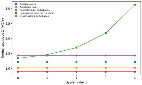
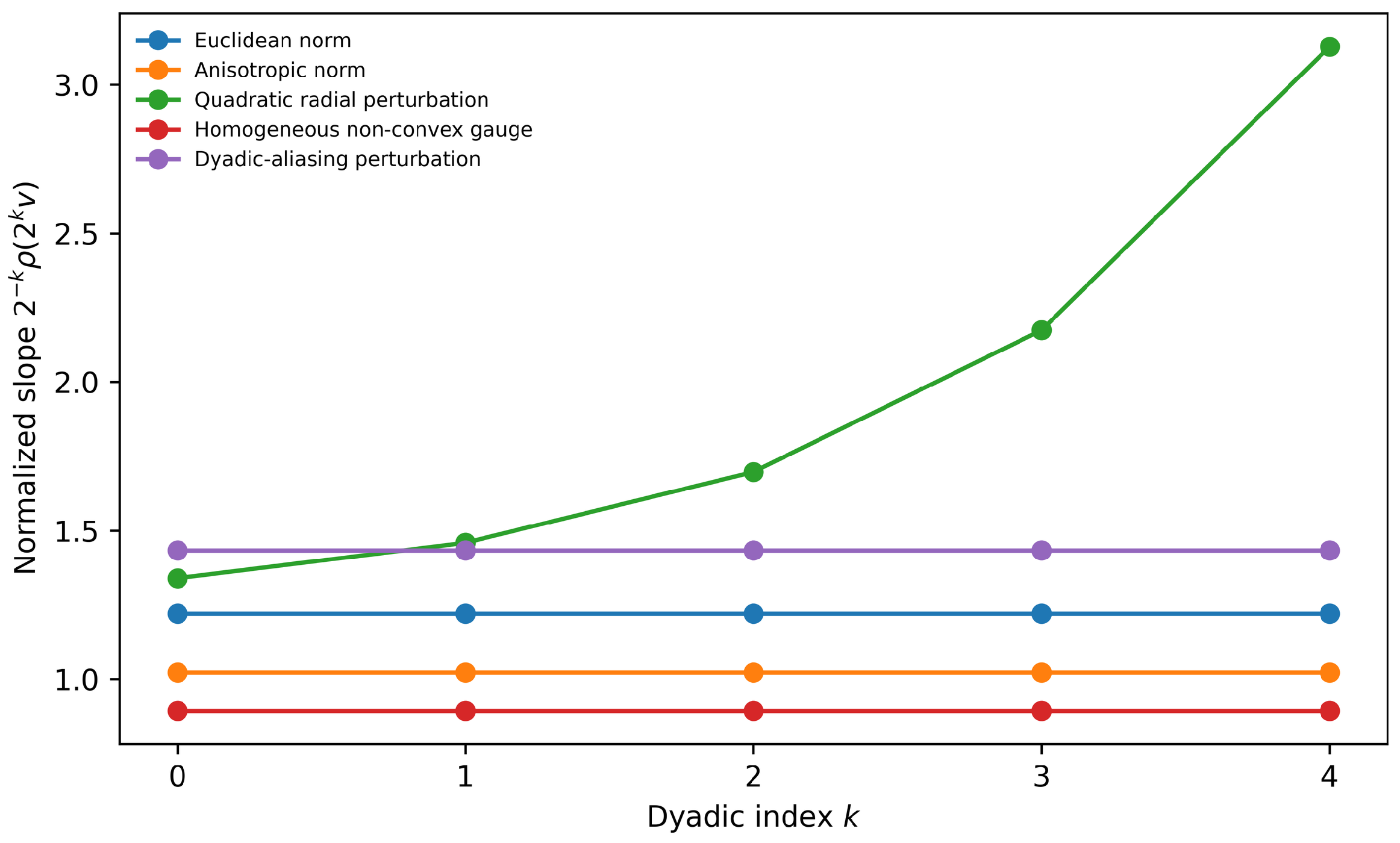
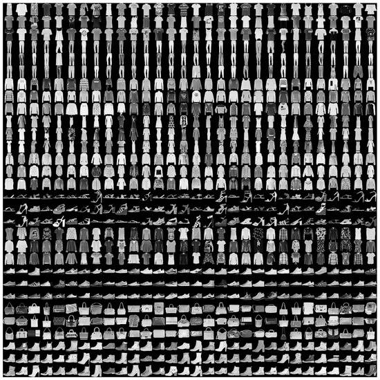
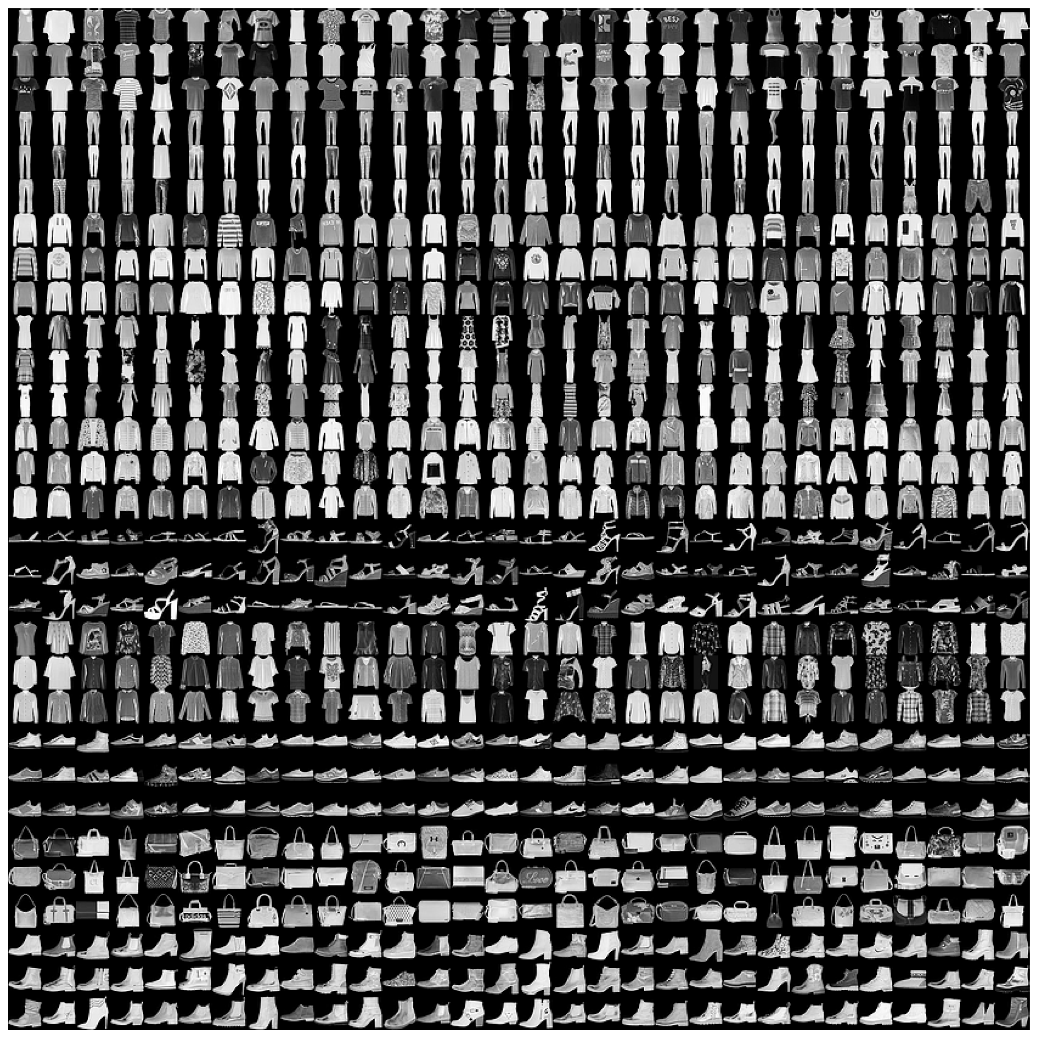
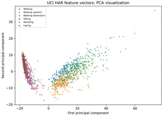
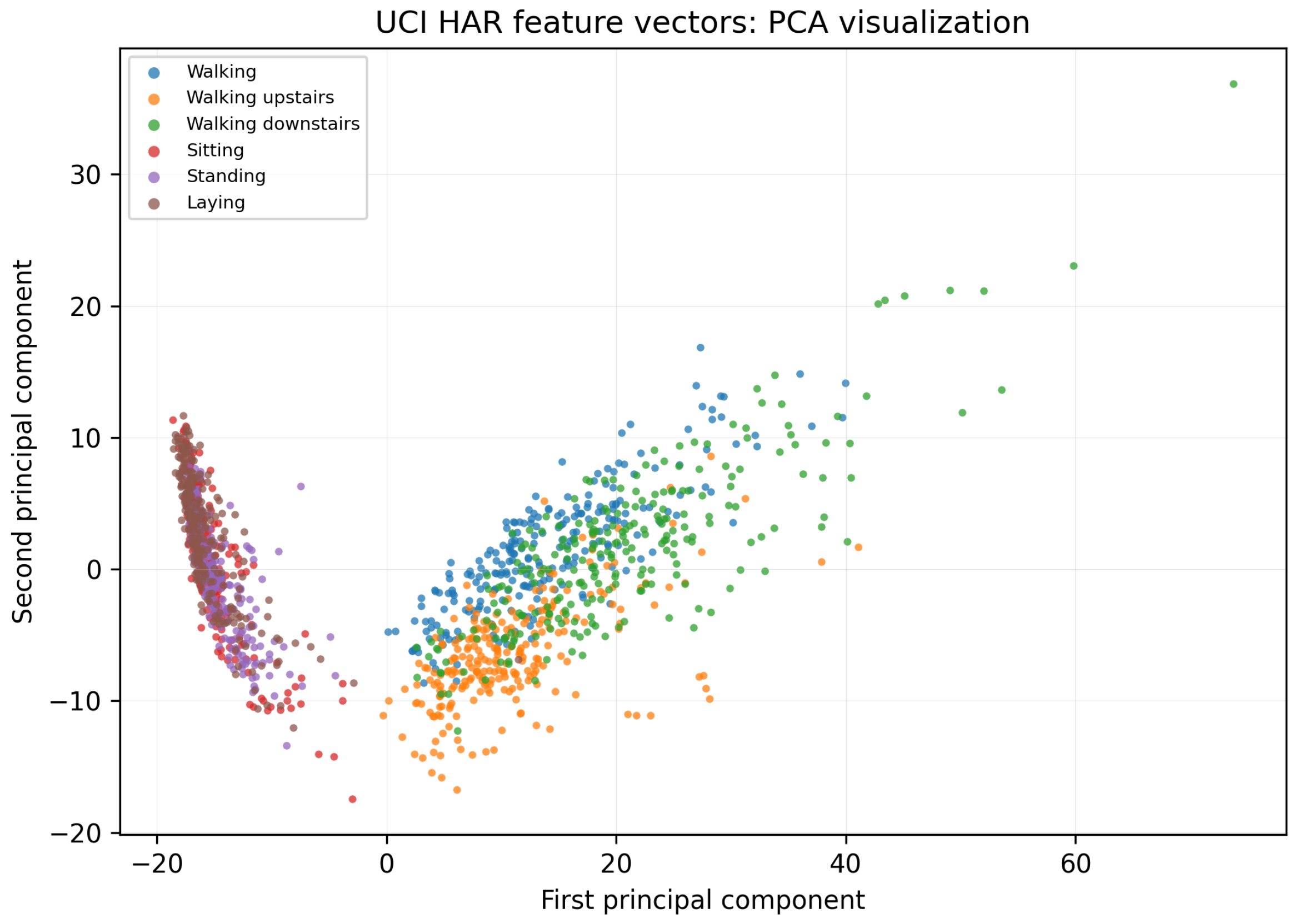
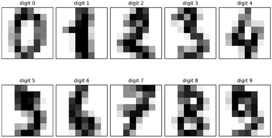
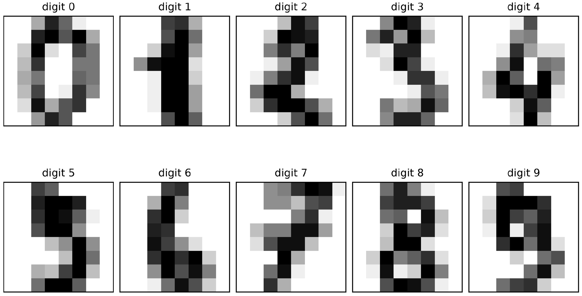
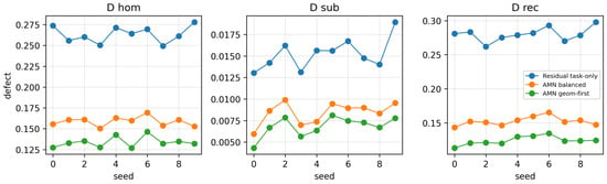
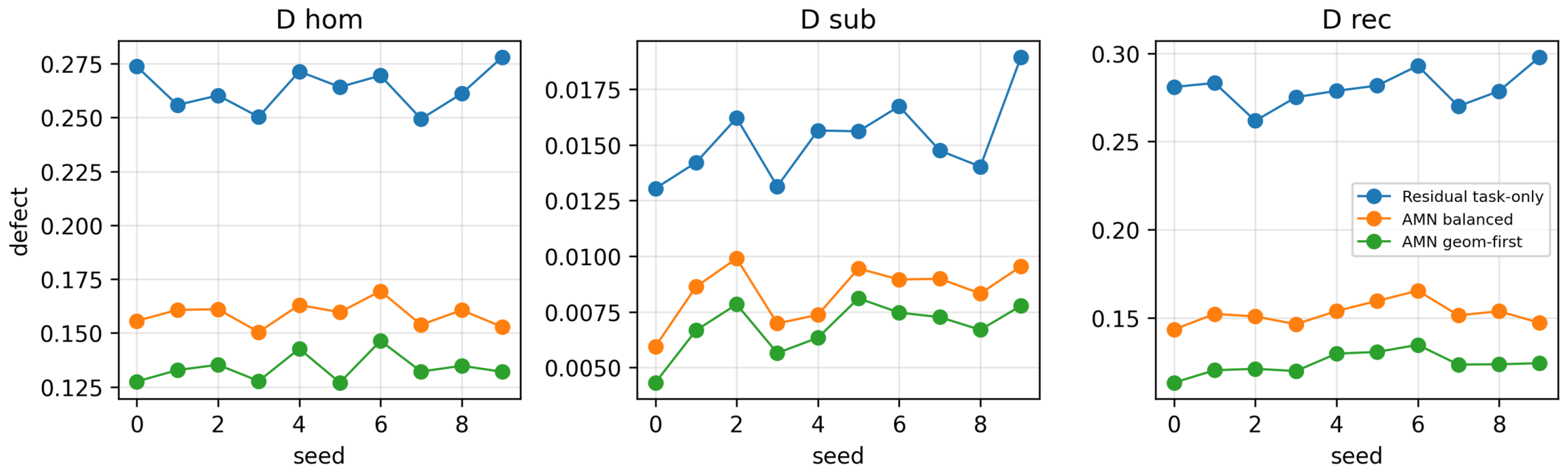
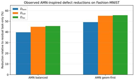
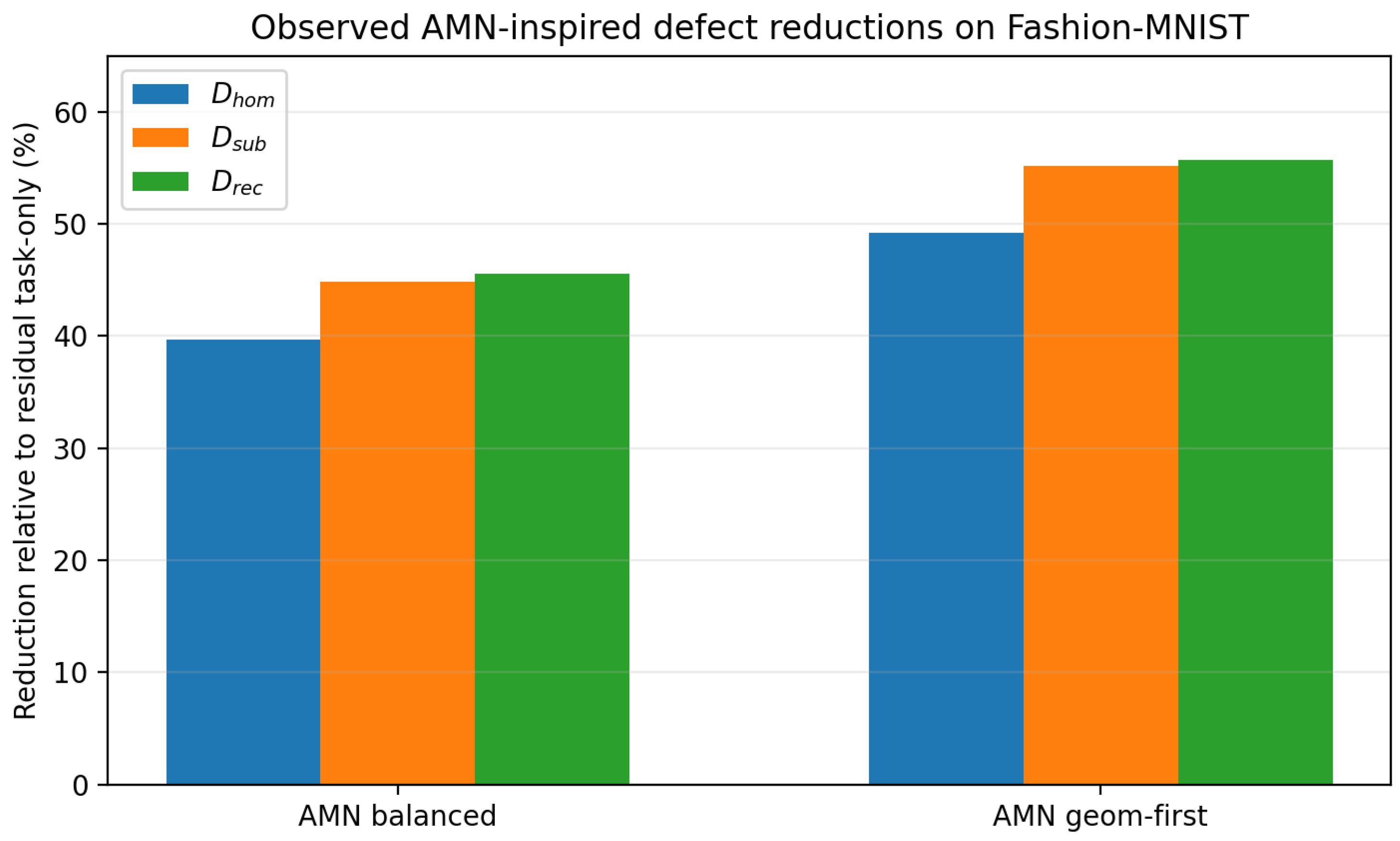
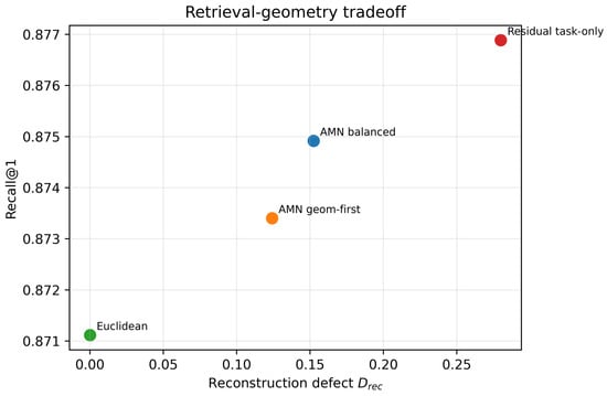
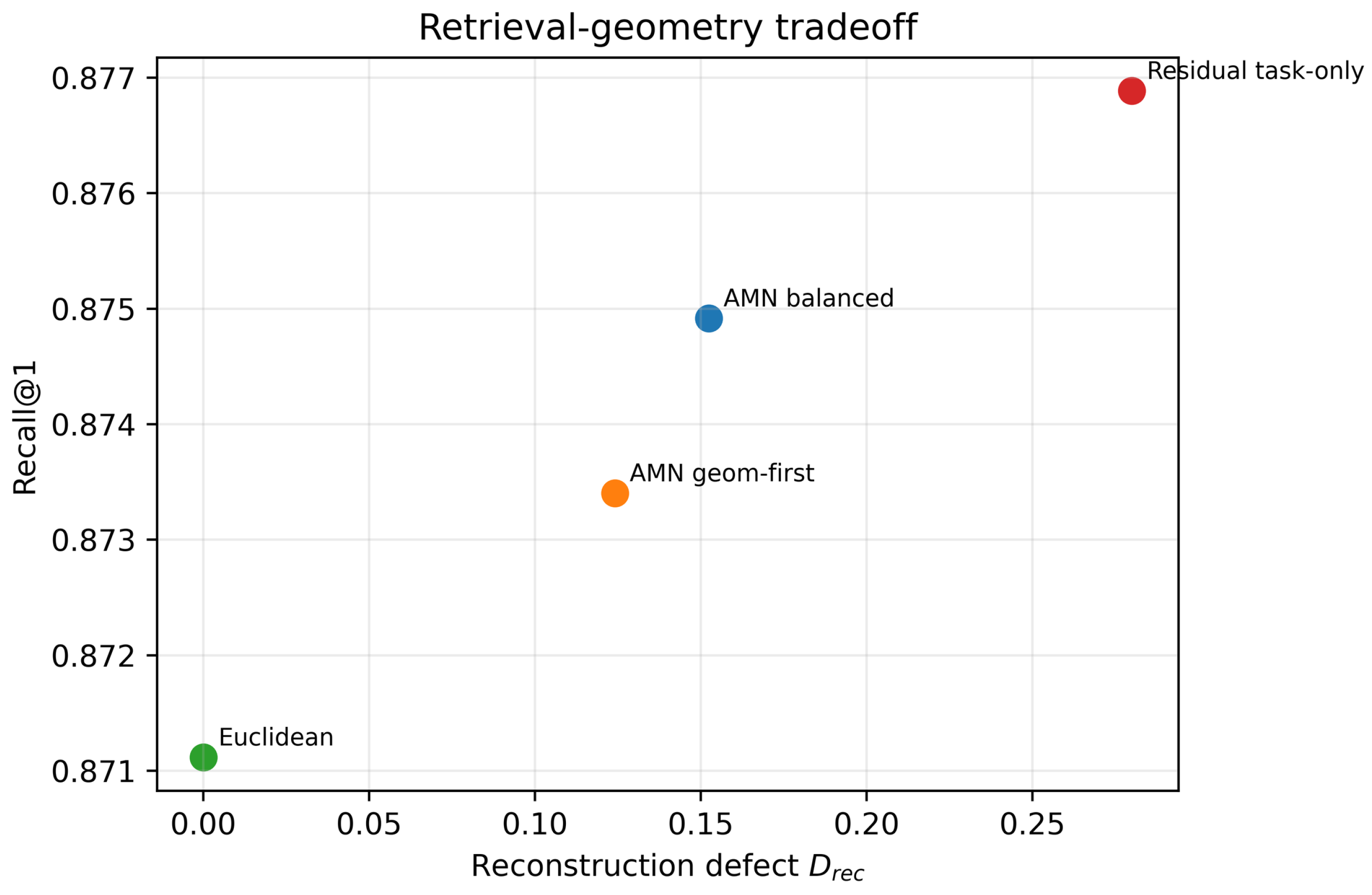
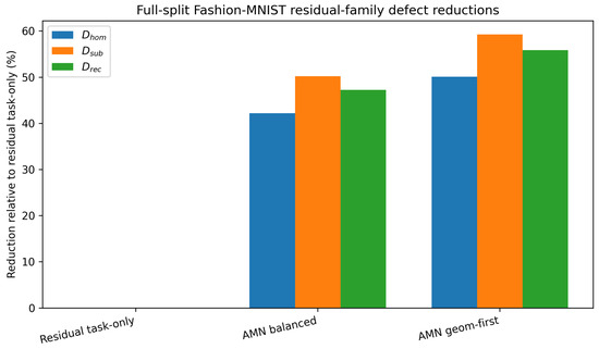
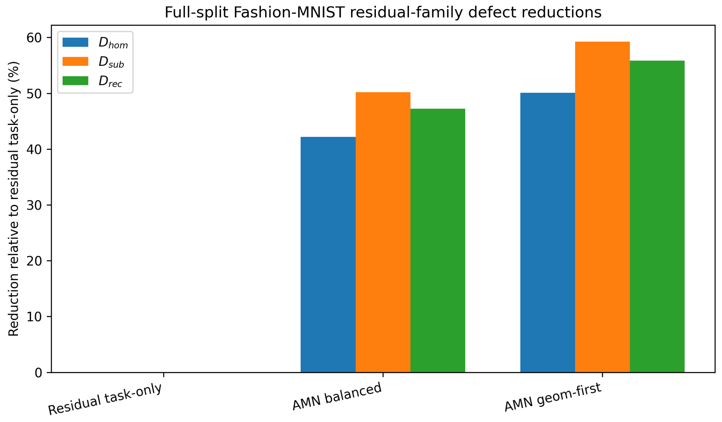
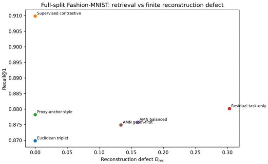
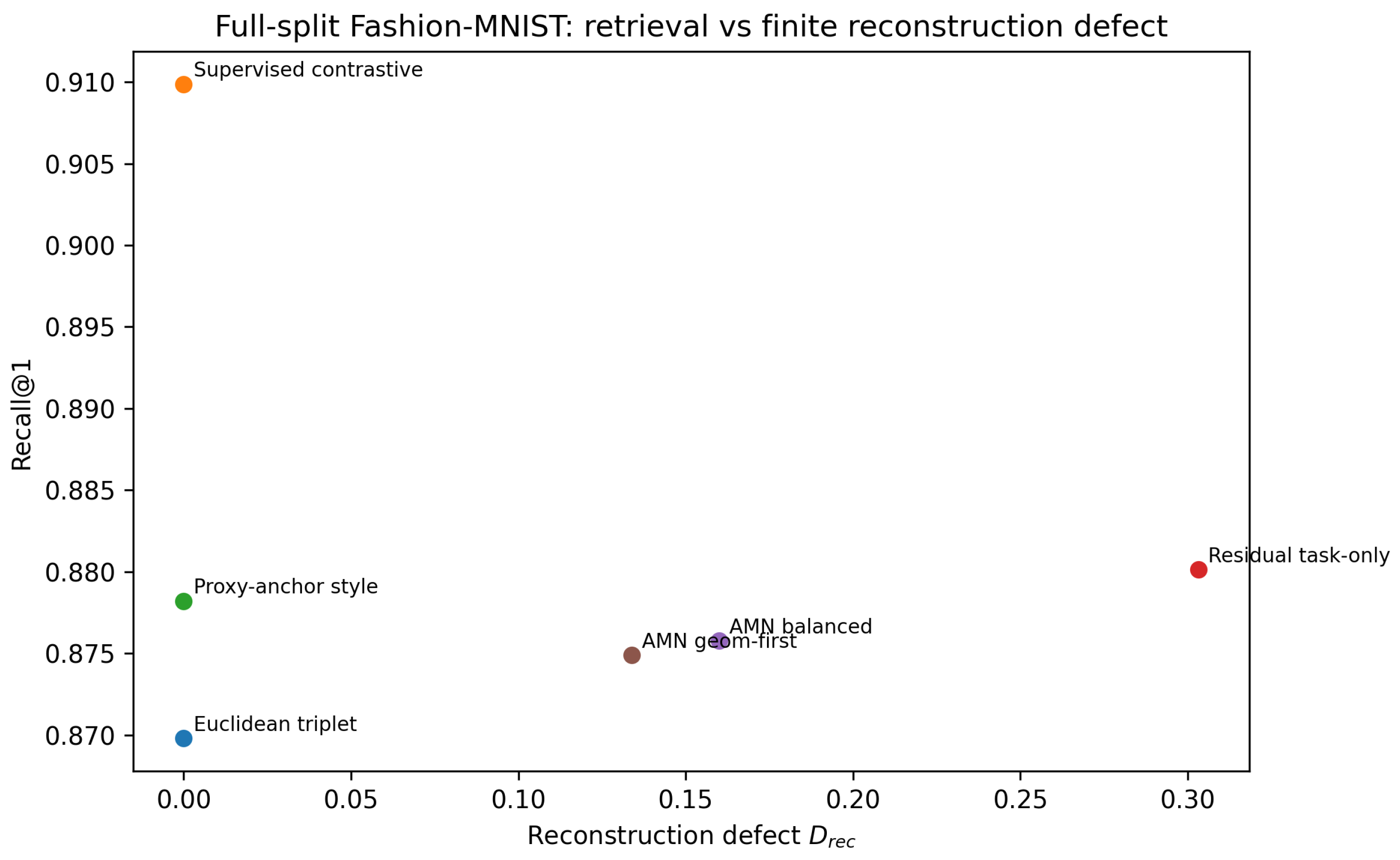
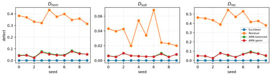
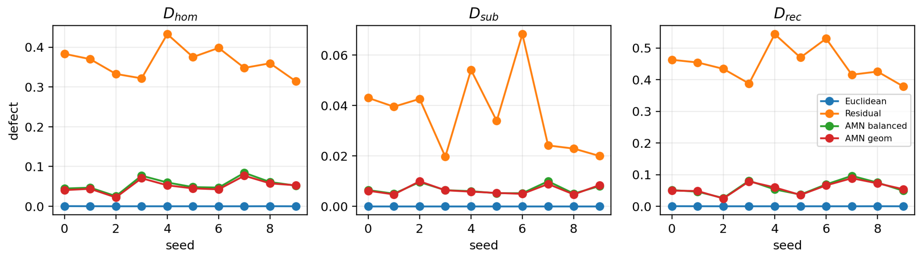
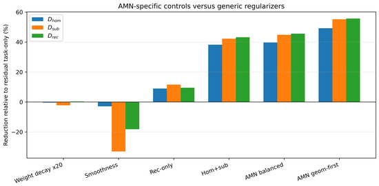
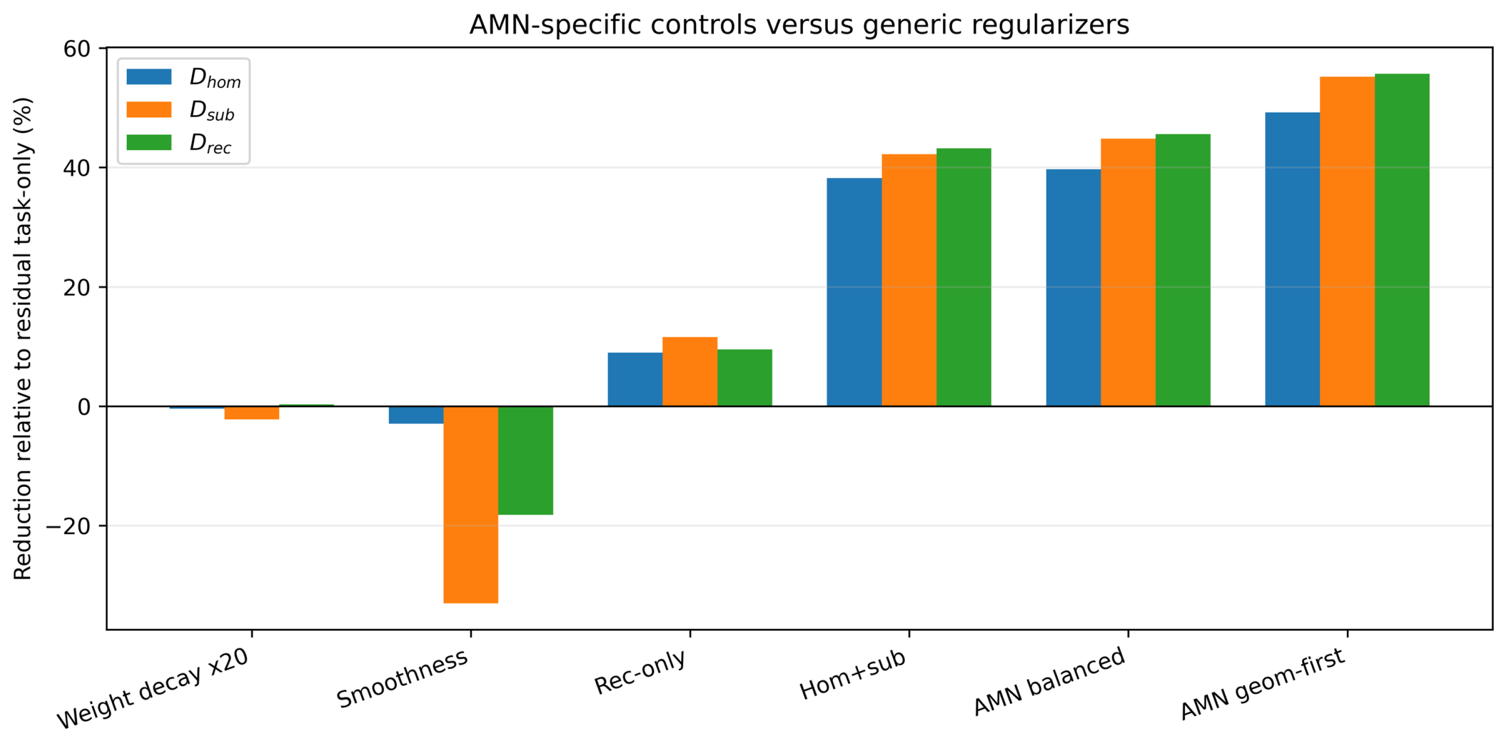

Disclaimer/Publisher’s Note: The statements, opinions and data contained in all publications are solely those of the individual author(s) and contributor(s) and not of MDPI and/or the editor(s). MDPI and/or the editor(s) disclaim responsibility for any injury to people or property resulting from any ideas, methods, instructions or products referred to in the content. |
© 2026 by the author. Licensee MDPI, Basel, Switzerland. This article is an open access article distributed under the terms and conditions of the Creative Commons Attribution (CC BY) license.