WAVE: Interpretable High-Dimensional Change Point Detection via Adaptive Weighted Variable Selection

Abstract

High-dimensional change point detection is a fundamental problem in modern statistical learning, particularly when distributional changes are driven by a small and unknown subset of variables. In heterogeneous settings, uniform aggregation across coordinates may suffer from signal dilution, because stable or noisy variables can mask the evidence carried by structurally unstable coordinates. Moreover, many existing procedures primarily focus on temporal localization and provide limited information about the variables responsible for a detected structural break. To address these challenges, we propose WAVE, a weighted adaptive variable selection procedure for interpretable change point detection. WAVE constructs variance-standardized global CUSUM evidence and locally standardized exponentially weighted evidence for each coordinate and then adaptively maps intervalwise coordinate evidence into a continuous weight vector. The learned weights strengthen coordinates with persistent or local evidence of change while downweighting nuisance coordinates with weak evidence. The resulting weighted scan statistic is calibrated by a residual moving block bootstrap that preserves temporal and cross-sectional dependence and re-applies the weighting rule within bootstrap samples to account for data-adaptive aggregation. Detected change points are further equipped with coordinate-level attribution through a multi-criteria fusion rule combining adaptive weights, local standardized effect sizes, and marginal testing evidence. Simulation studies show that WAVE achieves accurate localization and reliable support recovery in both single and multiple change point settings, particularly under sparse and heterogeneous alternatives. An empirical analysis of S&P 100 stock returns in 2020 further demonstrates that WAVE identifies economically meaningful market regime shifts with interpretable coordinate-level attribution.

1. Introduction

High-dimensional change point detection has become an indispensable tool in modern scientific and industrial data analysis. In finance, structural breaks in return dynamics, volatility proxies, and dependence measures are used to characterize changes in market risk and portfolio behavior [1]. In genomics, change point methods help localize copy number variations and other sequence-level structural alterations [2]. In environmental studies, they are used to detect shifts in climate records, pollution processes, and other temporally evolving systems [3,4]. In network traffic analysis, sparse changes in high-dimensional traffic streams may indicate anomalous or malicious behavior [5]. In industrial process control, change point methods support the real-time monitoring of operational variables and dynamic process intervals [6,7]. Despite this broad relevance, modern high-dimensional data pose substantial challenges for existing detection procedures.

A central difficulty is that the number of variables can be comparable to, or even larger than, the sample size. In this regime, classical low-dimensional change point methods often suffer from reduced detection power, unstable calibration, and limited interpretability. This difficulty is further intensified by variable heterogeneity. In many applications, only a small subset of coordinates undergoes structural change, whereas the remaining variables remain stable or contribute mainly noise. A method that aggregates all coordinates uniformly may therefore dilute the true signal. In addition, locating the temporal position of a change point is often insufficient for scientific interpretation, because practitioners also need to identify the variables that drive the structural change.

Most existing high-dimensional change point methods are based on cumulative sum (CUSUM) statistics. Let $X_i={(X_{i1},\dots ,X_{id})}^{\top }$ denote the ith observation of a d-dimensional sequence, where $i=1,\dots ,n$. For component $j=1,\dots ,d$ and candidate location $k=1,\dots ,n-1$, a standardized CUSUM statistic is commonly written as

$$C_{\gamma ,j}\left(k\right)={\left\{{\displaystyle \frac{k}{n}}\left(1-{\displaystyle \frac{k}{n}}\right)\right\}}^{-\gamma }{\displaystyle \frac{1}{\sqrt{n}}}{\displaystyle \frac{S_{kj}-\frac{k}{n}{S}_{nj}}{{\widehat{\sigma }}_j}},$$

where $S_{kj}={\sum }_{r=1}^k{X}_{rj}$, and ${\widehat{\sigma }}_j$ is an estimator of the marginal scale, or the long-run scale when serial dependence is present, of the jth component. The parameter $\gamma \in \{0,1/2\}$ controls the boundary weighting of candidate locations.

Representative $L_2$-based procedures include those in [8], which maximize the sum of squared CUSUM statistics over candidate locations. Related approaches were developed by [9,10]. Further extensions replace the CUSUM statistic with self-normalized U-statistics [11] or aggregate information jointly over temporal indices and dimensions [12,13]. These methods are powerful when many variables carry moderate signals, but they may be less effective under sparse alternatives because the contribution of a few changed coordinates can be overwhelmed by many inactive ones. By contrast, $L_{\infty }$-based procedures focus on the strongest marginal evidence. Ref. [1] studied the supremum of $|C_{0,j}\left(k\right)|$ over both time and coordinates, while [14] examined the maximum of $|C_{1/2,j}\left(k\right)|$ over variables and interior candidate locations. These approaches are sensitive to sparse and strong changes, but they may lose power when the signal is distributed across multiple coordinates.

Recent developments have extended high-dimensional change point inference in several directions. Ref. [15] studies distributional change point detection using $L_p$-norm-based U-statistics. For multiple change points, ref. [16] proposes a signal-screening-based local U-statistic method and establishes consistency for both the number and locations of changes. Beyond CUSUM-type procedures, ref. [17] develops a bootstrap moving-sum statistic, and [18] proposes a dimension-agnostic test for mean changes in weakly dependent multivariate time series. These contributions improve the flexibility and scope of high-dimensional change point analysis, but they do not directly provide a unified mechanism for variable-level interpretation under heterogeneous structural changes.

Several methods attempt to adapt high-dimensional change point detection to unknown sparsity patterns. Threshold-based sparse CUSUM procedures aggregate only those marginal CUSUM statistics that exceed a prespecified threshold [19,20]. These methods can be effective under sparse alternatives, but the thresholding step acts as a hard screening mechanism: a coordinate either contributes to the detection statistic or is excluded. Consequently, they do not naturally provide a continuous coordinate importance ranking for post-detection interpretation. Other adaptive aggregation methods combine or select among different global aggregation statistics [21,22]. Generalized $L_q$ aggregation interpolates between dense and sparse alternatives [2,22], and the DMS algorithm of [23] combines $L_2$ and $L_{\infty }$ evidence through Fisher’s method. These methods improve detection by adapting the global test statistic, but they do not directly learn a coordinate-specific weight vector that can be used for variable-level attribution.

Interpretability also requires identifying the variables that drive each detected structural change. Some recent studies have considered joint change point detection and variable selection. For example, ref. [24] uses group variance inflation factor regression to identify structural breaks in linear models, while ref. [25] develops a procedure for categorical data based on hierarchical log-linear models. In Bayesian settings, ref. [26] uses a latent probit model and reversible jump Markov chain Monte Carlo to explore change point configurations, and ref. [27] combines dynamic programming with exact Bayesian regression inference. These methods provide useful variable selection tools, but their formulations are often tied to specific regression, categorical, or Bayesian structures, or they treat localization and variable selection as separate inferential steps. Therefore, for high-dimensional mean change analysis, it is useful to develop a CUSUM-type procedure in which the evidence used for localization is systematically linked to coordinate-level attribution.

Motivated by these observations, we propose WAVE, a weighted adaptive variable selection procedure for interpretable change point detection. WAVE is designed as an evidence-coupled localization attribution framework for high-dimensional mean change analysis. It constructs hybrid coordinatewise change point evidence by combining variance-standardized full-interval CUSUM information with locally standardized exponentially weighted evidence and maps the resulting intervalwise evidence scores to a continuous coordinate weight vector. The learned weights form an adaptively weighted scan statistic for change point localization, while the same coordinatewise evidence is further used for bootstrap calibration, recursive segmentation, and post-detection active coordinate attribution.

The main contributions of this paper are fourfold. First, we construct a hybrid coordinatewise scan statistic that captures both sustained mean shifts and abrupt local changes. Second, we introduce an adaptive coordinate-weighting mechanism that provides a graded measure of coordinate importance, in contrast to hard thresholding in sparse CUSUM procedures. Third, we develop a residual moving block bootstrap calibration and recursive segmentation procedure that accounts for temporal dependence and the data-adaptive weighting step. Fourth, we propose a post-detection active coordinate identification rule that combines learned weights, local standardized effect sizes, and marginal testing evidence. Therefore, WAVE outputs estimated change point locations together with their associated active coordinate sets. Simulation studies and an empirical analysis of S&P 100 stock returns demonstrate its localization accuracy and variable-level interpretability in the examined settings.

2. Methodology

This section presents WAVE, a weighted adaptive procedure for high-dimensional mean change detection with coordinate-level attribution. In high-dimensional sequences, structural breaks are often sparse and heterogeneous, in the sense that only a small and unknown subset of coordinates is affected by the change. The inferential task therefore has two components. The first is to localize the change points, and the second is to identify the coordinates that contribute to each detected structural change. WAVE addresses this joint task by combining hybrid coordinatewise scan statistics, adaptive coordinate weighting, residual moving block bootstrap calibration, recursive segmentation, and post-detection active coordinate identification.

WAVE is formulated for mean change detection. When applied directly to raw observations, it does not target a pure variance change with an unchanged mean. Variance or covariance changes can instead be examined by applying WAVE to transformed features, such as centered squared observations or selected cross-products, which convert second-order changes into mean changes in the transformed sequence.

2.1. Problem Formulation

Let ${\left\{{\mathbf{X}}_t\right\}}_{t=1}^T$ be a d-dimensional stochastic process, where ${\mathbf{X}}_t={(X_{1,t},\dots ,X_{d,t})}^{\top }\in {\mathbb{R}}^d$ denotes the observation vector at time t. We consider the high-dimensional piecewise constant mean model

$${\mathbf{X}}_t={\mathit{\mu }}_t+{\mathit{ϵ}}_t,t=1,\dots ,T,$$

(1)

where ${\mathit{\mu }}_t=\mathbb{E}\left({\mathbf{X}}_t\right)$ is the mean vector, and ${\mathit{ϵ}}_t={\mathbf{X}}_t-{\mathit{\mu }}_t$ is a zero-mean error process. The mean sequence is assumed to be piecewise constant. Specifically, there exist an unknown number of change points $1<{\tau }_1<\dots <{\tau }_K<T$ such that the mean vector is constant within each segment and changes across adjacent segments. The error process is allowed to exhibit both serial dependence and cross-sectional dependence.

For a generic interval $[s,e]$, WAVE considers whether the mean vector remains constant throughout the interval or changes once at an unknown location within the interval. This local testing problem is embedded in recursive segmentation. If a change is detected, the interval is split at the estimated location, and the same procedure is applied to the resulting subintervals.

When an interval contains a single change point $\tau$, let $\mathit{\delta }$ denote the difference between the post-change and pre-change mean vectors. The active coordinate set is the set of coordinates for which the corresponding entry of $\mathit{\delta }$ is nonzero. In sparse high-dimensional settings, this active set is much smaller than the ambient dimension, which motivates recovering the affected coordinates in addition to localizing the change point.

Table 1. Summary of main notation used in WAVE.

Notation	Meaning
${\mathbf{X}}_t\in {\mathbb{R}}^d$	Observation vector at time t
T and d	Sequence length and dimension
${\mathit{\mu }}_t$	Mean vector at time t
${\tau }_k$	True change point location
$\mathit{\delta }$	Mean shift vector across a change point
$\mathcal{S}$	True active coordinate set
$[s,e]$	Current interval in recursive segmentation
${\mathcal{B}}_{s,e}$	Admissible candidate set on $[s,e]$
$T_j^{\mathrm{glo}}(b;s,e)$	Variance-standardized intervalwise CUSUM statistic for coordinate j
$T_j^{\mathrm{loc}}(b;s,e)$	Locally standardized exponentially weighted statistic for coordinate j
$T_j(b;s,e)$	Hybrid coordinatewise scan statistic
$C_j(s,e)$	Intervalwise evidence score for coordinate j
$w_{j,s:e}^{(*)}$	Observed adaptive weight for coordinate j on $[s,e]$
$Q_{s,e}\left(b\right)$	Weighted scan statistic at candidate location b
${\widehat{\tau }}_{s,e}$	Estimated change point on interval $[s,e]$
${\mathbb{M}}_{s,e}$	Observed maximum weighted scan statistic
${\mathbb{M}}_{s,e}^{\star \left(r\right)}$	Bootstrap maximum statistic in replication r
${\widehat{c}}_{\alpha }(s,e)$	Bootstrap critical value
$\widehat{\mathcal{D}}\left(\widehat{\tau }\right)$	Estimated active coordinate set at detected change point $\widehat{\tau }$

summarizes the main notation used throughout the proposed method.

2.2. Overview of WAVE

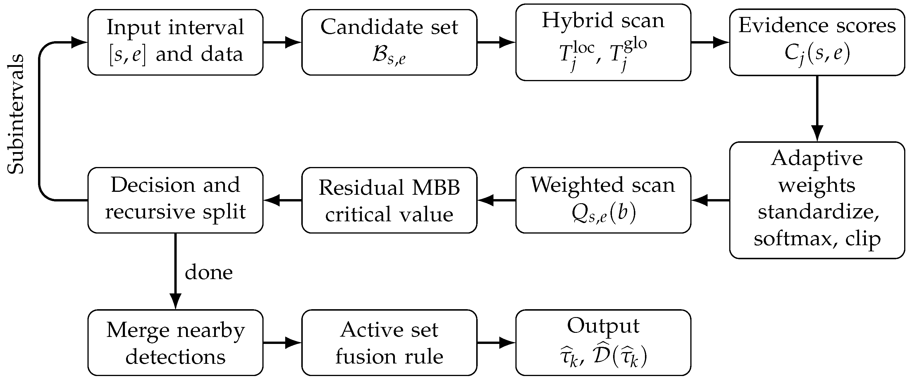
The complete workflow is shown in Figure 1. For each candidate interval, WAVE constructs an admissible set of interior split locations and computes hybrid coordinatewise scan statistics. These coordinatewise statistics are summarized over candidate locations to obtain intervalwise evidence scores, which are then transformed into adaptive coordinate weights. The weighted scan statistic is calibrated by a residual moving block bootstrap, where the same weighting rule is re-applied within each bootstrap sample by default. Significant detections are used to split the interval recursively. After the recursive search, nearby detections are merged, and a multi-criteria fusion rule is applied to identify the active coordinates associated with each retained change point.

Algorithm 1 summarizes the full procedure. The main components are detailed in Section 2.3, Section 2.4, Section 2.5 and Section 2.6.

Algorithm 1 WAVE Algorithm

1: Input High-dimensional time series $\mathbf{X}=({\mathbf{X}}_1,\dots ,{\mathbf{X}}_T)$, local window radius h, trimming parameter $\rho$, hybrid parameter $\lambda$, exponential decay parameter r, significance levels $\left\{{\alpha }_{\ell }\right\}$, moving block length ${\ell }_{\mathrm{blk}}$, number of bootstrap replications B, weight-temperature parameter ${\alpha }_w$, clipping constants, minimum separation distance ${\Delta }_{min}$, active-set parameters, and maximum recursion depth $D_{max}$. 2: Initialize a queue $\mathcal{Q}$ with $\left(\right[1,T],0)$ and initialize $\widehat{\mathcal{T}}=\varnothing$. 3: while $\mathcal{Q}$ is not empty do 4:    Pop an interval and its recursion level $\left(\right[s,e],\ell )$ from $\mathcal{Q}$. 5:    Construct the admissible candidate set ${\mathcal{B}}_{s,e}$. 6:    if ${\mathcal{B}}_{s,e}=\varnothing$ or $\ell >D_{max}$ then 7:      continue 8:    end if 9:    Compute the observed adaptive weight vector ${\mathit{w}}_{s,e}^{(*)}$ from the intervalwise coordinate evidence scores.   10:    Compute the weighted scan statistic $Q_{s,e}\left(b\right)$ and the candidate change point ${\widehat{\tau }}_{s,e}$ using (7) and (8).   11:    Compute the observed maximum statistic ${\mathbb{M}}_{s,e}$.   12:    Generate B residual moving block bootstrap samples under the local null model.   13:    For each bootstrap sample, recompute the hybrid coordinatewise scan statistics, recompute the adaptive weights by the same weighting rule, and obtain ${\mathbb{M}}_{s,e}^{\star \left(r\right)}$, $r=1,\dots ,B$.   14:    Compute the bootstrap critical value ${\widehat{c}}_{\alpha }(s,e)$.   15:    if ${\mathbb{M}}_{s,e}>{\widehat{c}}_{\alpha }(s,e)$ then   16:      Add $({\widehat{\tau }}_{s,e},{\mathit{w}}_{s,e}^{(*)},{\mathbb{M}}_{s,e},[s,e])$ to $\widehat{\mathcal{T}}$.   17:      if $\ell <D_{max}$ then   18:         Add $([s,{\widehat{\tau }}_{s,e}],\ell +1)$ and $([{\widehat{\tau }}_{s,e}+1,e],\ell +1)$ to $\mathcal{Q}$.   19:      end if   20:    end if   21: end while   22: Merge detected change points in $\widehat{\mathcal{T}}$ that are closer than ${\Delta }_{min}$, retaining the one with the larger observed maximum statistic.   23: for each retained detection $({\widehat{\tau }}_k,{\mathit{w}}_k^{(*)},{\mathbb{M}}_{s_k,e_k},[s_k,e_k])$ do   24:    Apply the multi-criteria fusion rule in (10) to obtain $\widehat{\mathcal{D}}\left({\widehat{\tau }}_k\right)$.   25: end for   26: Output The sorted set of estimated change points and their active coordinate sets $\{({\widehat{\tau }}_k,\widehat{\mathcal{D}}({\widehat{\tau }}_k))\}$.

2.3. Hybrid Coordinatewise Scan Statistic

The first step of WAVE constructs a coordinatewise statistic for assessing mean change evidence at each candidate location. On an interval $[s,e]$, the candidate locations are restricted to interior points so that both sides of a candidate split contain at least a prescribed number of observations. This minimum side length is determined by the local window size and the trimming parameter. The restriction removes unstable boundary splits and ensures that the local windows used below are well defined.

For coordinate j and candidate location b, let ${\overline{X}}_{j,s:b}$ and ${\overline{X}}_{j,b+1:e}$ denote the empirical means before and after b on the interval $[s,e]$. Let ${\widehat{\sigma }}_{j,s:e}^2$ be a positive coordinatewise scale estimator on $[s,e]$. For weakly dependent data, ${\widehat{\sigma }}_{j,s:e}^2$ may be the sample variance, whereas for serially dependent data, a heteroskedasticity- and autocorrelation-consistent or block-based long-run variance estimator is preferred. The variance-standardized intervalwise CUSUM statistic is

$$T_j^{\mathrm{glo}}(b;s,e)={\displaystyle \frac{(b-s+1)(e-b)}{e-s+1}}{\displaystyle \frac{{\left({\overline{X}}_{j,s:b}-{\overline{X}}_{j,b+1:e}\right)}^2}{{\widehat{\sigma }}_{j,s:e}^2+{\epsilon }_{\sigma }}},$$

(2)

where ${\epsilon }_{\sigma }>0$ is a small numerical constant. Scale standardization makes the statistic comparable across coordinates.

To capture more localized changes, WAVE also uses an exponentially weighted local contrast. Around each candidate split, the method forms a left local window and a right local window of radius proportional to h. Within each window, observations closer to the candidate split receive larger exponential weights, controlled by the decay parameter r. Let ${\mu }_j^{-}(b;s,e)$ and ${\mu }_j^{+}(b;s,e)$ denote the resulting weighted local means, and let ${\widehat{v}}_{j,-}(b;s,e)$ and ${\widehat{v}}_{j,+}(b;s,e)$ denote the corresponding weighted local variance estimates. The locally standardized squared contrast is

$$T_j^{\mathrm{loc}}(b;s,e)={\displaystyle \frac{{\left\{{\mu }_j^{-}(b;s,e)-{\mu }_j^{+}(b;s,e)\right\}}^2}{{\widehat{v}}_{j,-}(b;s,e)\parallel {\mathit{\omega }}^{-}{\left(b\right)\parallel }_2^2+{\widehat{v}}_{j,+}(b;s,e){\parallel {\mathit{\omega }}^{+}\left(b\right)\parallel }_2^2+{\epsilon }_{\sigma }}},$$

(3)

where ${\mathit{\omega }}^{-}\left(b\right)$ and ${\mathit{\omega }}^{+}\left(b\right)$ are the normalized exponential weight vectors in the left and right local windows. This statistic measures a local signal-to-noise ratio for coordinate j around the candidate location.

The hybrid coordinatewise scan statistic is

$$T_j(b;s,e)=\lambda T_j^{\mathrm{loc}}(b;s,e)+(1-\lambda )T_j^{\mathrm{glo}}(b;s,e),0\le \lambda \le 1.$$

(4)

Larger values of $\lambda$ emphasize local evidence, whereas smaller values give greater weight to intervalwise cumulative evidence. When the interval is clear from context, we write $T_j\left(b\right)$ for $T_j(b;s,e)$.

Because WAVE is based on CUSUM-type statistics, the scaling and quality of the input series affect both the scan statistics and the learned weights. In applications with outliers or heavy-tailed observations, robust centering and scaling are recommended before computing the coordinatewise statistics. If some coordinates are measured with lower precision, reliability-adjusted scaling or coordinate-specific variance estimates can be used to reduce the chance that large weights are driven by measurement noise.

2.4. Adaptive Coordinate Weighting and Weighted Scan Statistic

The hybrid statistic $T_j(b;s,e)$ measures the change point evidence of coordinate j at candidate location b. WAVE aggregates these coordinatewise statistics in a way that adapts to the unknown sparsity pattern of the change. Instead of assigning equal importance to all coordinates, WAVE learns an interval-specific weight vector from the coordinatewise evidence and then uses this vector to construct an adaptively weighted scan statistic.

For each coordinate $j=1,\dots ,d$, define the intervalwise evidence score

$$C_j(s,e)=\underset{b\in {\mathcal{B}}_{s,e}}{max}{T}_j(b;s,e).$$

(5)

The score $C_j(s,e)$ records the strongest coordinatewise evidence over the admissible candidate locations. It is therefore a location-adaptive summary of whether coordinate j shows evidence of a mean change somewhere within the current interval.

The evidence scores are standardized across coordinates on the current interval. Very small standardized scores are truncated from below for numerical stability, and the resulting values are mapped to preliminary weights by a softmax transformation:

$${\tilde{w}}_j={\displaystyle \frac{exp({\alpha }_w{\check{C}}_j)}{{\sum }_{\ell =1}^{d}exp({\alpha }_w{\check{C}}_{\ell })}},j=1,\dots ,d,$$

(6)

where ${\check{C}}_j$ denotes the truncated standardized evidence score, and ${\alpha }_w>0$ controls the concentration of the weight vector. Larger values of ${\alpha }_w$ produce more concentrated weights, whereas smaller values produce weights closer to uniform aggregation.

The preliminary weights are then clipped to avoid degeneracy and renormalized to sum to one. The final interval-specific weight vector is denoted by ${\mathit{w}}_{s,e}^{(*)}={(w_{1,s:e}^{(*)},\dots ,w_{d,s:e}^{(*)})}^{\top }$. This one-step weighting rule is deterministic once the coordinatewise scan statistics have been computed. Since the evidence scores do not depend on a current or previous weight vector, no iterative weight optimization is required.

The weighting mechanism is monotone in the coordinatewise evidence scores, up to the stabilizing clipping step. If coordinate j is active, its CUSUM-type statistic tends to increase near the true change point, so its evidence score contains a signal component in addition to stochastic fluctuation. If coordinate j is inactive, its evidence score is mainly noise-driven. Thus, when active and inactive coordinates are sufficiently separated in evidence scores, active coordinates tend to receive larger adaptive weights.

Using the adaptive weights, WAVE defines the weighted scan statistic

$$Q_{s,e}\left(b\right)={\displaystyle \sum _{j=1}^d}{w}_{j,s:e}^{(*)}{T}_j(b;s,e),b\in {\mathcal{B}}_{s,e}.$$

(7)

The estimated change point on the interval $[s,e]$ is

$${\widehat{\tau }}_{s,e}=arg\underset{b\in {\mathcal{B}}_{s,e}}{max}{Q}_{s,e}\left(b\right),$$

(8)

with ties resolved by choosing the smallest maximizer.

The statistic $Q_{s,e}\left(b\right)$ is a data-adaptive aggregation of coordinatewise CUSUM-type evidence. Informative coordinates contribute more to the scan through larger weights, whereas stable or noise-dominated coordinates are downweighted. On an interval containing a single change point, a stronger weighted signal over the active coordinates increases the gap between the scan value near the true change point and the scan values at other candidate locations.

2.5. Bootstrap Calibration and Recursive Segmentation

The maximum weighted scan statistic does not generally have a tractable null distribution in high-dimensional time series, because it is affected by serial dependence, cross-sectional dependence, maximization over candidate locations, and data-adaptive weighting. WAVE therefore uses a residual moving block bootstrap to obtain a data-dependent critical value.

For an interval $[s,e]$, let ${\mathbb{M}}_{s,e}={max}_{b\in {\mathcal{B}}_{s,e}}{Q}_{s,e}\left(b\right)$ denote the observed maximum weighted scan statistic. To approximate its null distribution, WAVE first fits the local null model by subtracting the interval mean from all observations in $[s,e]$. Overlapping vector-valued residual blocks of length ${\ell }_{\mathrm{blk}}$ are then sampled with replacement and concatenated to form a bootstrap residual sequence of length $n_{s,e}$. The sequence is recentered and shifted by the interval mean. This residual moving block bootstrap preserves local serial dependence within blocks and cross-sectional dependence across coordinates.

For each bootstrap sample, WAVE recomputes the hybrid coordinatewise scan statistics and re-applies the same adaptive weighting rule used for the observed sample. The resulting bootstrap maximum statistic is the maximum of the bootstrap weighted scan over the admissible candidate locations. Relearning the weights inside each bootstrap replication is important because the observed statistic is not based on a fixed weight vector. It better mimics the data-adaptive nature of WAVE and reduces the risk of anti-conservative calibration caused by selecting high-noise coordinates under the null.

The empirical upper quantile of the bootstrap maximum statistics is used as the critical value for the interval-level test. Specifically, ${\widehat{c}}_{\alpha }(s,e)$ is the empirical $(1-{\alpha }_{\ell })$ quantile of $\{{\mathbb{M}}_{s,e}^{\star \left(r\right)}:r=1,\dots ,B\}$. A change point is declared when the observed maximum weighted scan statistic exceeds this bootstrap critical value. This calibration step uses the same adaptive weighting rule in the observed and bootstrap samples and does not introduce additional stabilization parameters.

A change point is declared on $[s,e]$ if

$${\mathbb{M}}_{s,e}>{\widehat{c}}_{\alpha }(s,e).$$

(9)

If this inequality holds, the estimated location is ${\widehat{\tau }}_{s,e}$, and the interval is split into $[s,{\widehat{\tau }}_{s,e}]$ and $[{\widehat{\tau }}_{s,e}+1,e]$. The same procedure is then applied recursively to the two subintervals. If the inequality does not hold, the interval is treated as stationary. After the recursive search, nearby detections are merged, retaining the detection with the larger observed maximum statistic.

Because the bootstrap is constructed from residuals under the local null model, its validity is the most direct under $H_0$. When a strong change is present on the interval, the residual distribution may still contain some change-induced heterogeneity, which can make the bootstrap threshold conservative. Recursive segmentation mitigates this issue in practice by removing dominant changes and applying subsequent tests to shorter and more homogeneous subintervals.

2.6. Active Coordinate Identification

After a change point $\widehat{\tau }$ has been detected and validated, WAVE estimates the associated active coordinate set $\widehat{\mathcal{D}}\left(\widehat{\tau }\right)$. Because a single screening criterion may be unstable in high-dimensional settings, WAVE combines three complementary sources of evidence.

The first source is a local standardized effect size, computed by comparing local means immediately before and after $\widehat{\tau }$ for each coordinate. A robust threshold, based on a fixed lower bound together with a median-plus-MAD criterion across coordinates, is used to form the effect size set ${\mathcal{D}}_{\mathrm{eff}}$. This avoids selecting a coordinate solely because it is among the largest when all local effects are weak.

The second source is the adaptive weight vector associated with the detected change. Coordinates are sorted by their learned weights, and the weight-based set ${\mathcal{D}}_{\mathrm{weight}}$ is obtained by combining an elbow rule in the ordered weights with a cumulative weight rule. This construction avoids choosing too few coordinates when the signal is spread across several coordinates and avoids choosing too many when the weights are sharply concentrated.

The third source is marginal testing evidence. For each coordinate, WAVE compares the observations in local windows before and after $\widehat{\tau }$. When serial dependence is present, the marginal comparison should use a dependence-robust standard error or a local block bootstrap calibration. The resulting marginal p values are adjusted for multiple testing using a false discovery rate procedure, leading to a testing-based set ${\mathcal{D}}_t$.

The final active set is obtained by majority voting:

$$\widehat{\mathcal{D}}\left(\widehat{\tau }\right)=\left\{j:\mathbf{1}\{j\in {\mathcal{D}}_{\mathrm{eff}}\}+\mathbf{1}\{j\in {\mathcal{D}}_{\mathrm{weight}}\}+\mathbf{1}\{j\in {\mathcal{D}}_t\}\ge 2\right\}.$$

(10)

The majority rule requires support from at least two sources of evidence. This reduces the chance of selecting a coordinate solely because of an isolated local fluctuation, an unstable adaptive weight, or a marginally significant test result.

The resulting set $\widehat{\mathcal{D}}\left(\widehat{\tau }\right)$ provides the coordinate-level attribution of the detected structural change. It should be interpreted as a statistical estimate of the coordinates contributing to the weighted scan statistic, rather than as a causal explanation of the change. Exact support recovery would require active and inactive coordinates to be separated in terms of local effect size, learned weight ranking, and marginal testing evidence. The majority voting rule reduces dependence on any single evidence source and makes the estimated active set more stable in finite samples.

3. Simulation Studies

We conduct simulation studies to evaluate the finite sample performance of WAVE for high-dimensional mean change detection with coordinate-level attribution. The main experiments compare WAVE with benchmark procedures in representative single- and multiple-change-point settings. The sensitivity experiments then examine the effects of the hybrid parameter, bootstrap size, dependence structure, signal strength, and the active coordinate voting rule. The goal is to assess WAVE both as a localization procedure and as a method for coordinate-level statistical attribution.

3.1. Main Experiments

3.1.1. Data-Generating Mechanism

We generate high-dimensional time series from the piecewise constant mean model $Y_t={\mathit{\mu }}_t+{\mathit{\epsilon }}_t$, $t=1,\dots ,T$, where $Y_t\in {\mathbb{R}}^d$, and $T=500$. The mean vector changes at $K\in \{1,2\}$ locations sampled from the central region $[0.2T,0.8T]$ subject to a minimum spacing constraint. The dimension is varied over $d\in \{50,100,200\}$.

In the main comparisons, the active coordinate proportion is fixed at $\pi =0.20$. Thus, for each change point, the active set has size $s_d=max\{1,\lfloor d\pi \rfloor \}$. For each active coordinate, the jump size is sampled independently from $\mathcal{U}(0.7\Delta ,1.3\Delta )$ and assigned a random sign. The main comparison tables use $\Delta =1.20$, representing a relatively strong signal. Inactive coordinates have no mean shift.

The main experiments are conducted under cross-sectionally correlated Gaussian noise generated from a common factor structure. This setting is intended to represent high-dimensional applications in which coordinates are correlated at the same time point. The number of Monte Carlo replications and bootstrap replications is reported with the corresponding results.

3.1.2. Competing Methods

We compare WAVE with three benchmark procedures appearing in the simulation tables. DCSB denotes the double CUSUM binary segmentation method for high-dimensional panel change point detection [20]. DenseCUSUM is our implemented dense CUSUM aggregation baseline, which sums squared standardized coordinatewise CUSUM statistics across all coordinates [9]. SBS denotes the sparsified binary segmentation method for high-dimensional multiple change point detection [19]. WAVE and DCSB return coordinate-level support estimates, whereas DenseCUSUM and SBS are used as localization benchmarks.

For WAVE, we use $\lambda =0.6$, ${\alpha }_w=0.3$, and $r=0.95$. The local window is set to $h/T=0.05$ for the single-change setting and $h/T=0.07$ for the two-change setting. The maximum recursion depth is capped at one and two, respectively. These settings separate the single-change and two-change simulation regimes and do not use the true change point locations.

3.1.3. Evaluation Metrics

Let ${\mathcal{T}}_i$ and ${\widehat{\mathcal{T}}}_i$ denote the true and estimated change point sets in replication i. A true change point is counted as detected if at least one estimated change point lies within the tolerance radius ${\epsilon }_T=2log\left(T\right)$. Detection is the average proportion of true change points recovered within this tolerance. Exact is the proportion of replications in which the estimated number of change points equals the true number. Est. Num. denotes the average estimated number of change points and is used to assess under-segmentation and over-segmentation.

Localization accuracy is evaluated by the mean absolute error

$$\mathrm{MAE}={\displaystyle \frac{1}{M_{\mathrm{rep}}K}}{\displaystyle \sum _{i=1}^{M_{\mathrm{rep}}}}\sum _{\tau \in {\mathcal{T}}_i}\left|{\widehat{\tau }}_{\mathrm{closest}}-\tau \right|,$$

where ${\widehat{\tau }}_{\mathrm{closest}}$ is the estimated change point closest to $\tau$. If no change point is detected in a replication, a conservative penalty equal to T is used. We also compute the Hausdorff distance

$$d_H(\mathcal{T},\widehat{\mathcal{T}})=max\left\{\underset{\tau \in \mathcal{T}}{sup}\underset{\widehat{\tau }\in \widehat{\mathcal{T}}}{inf}|\tau -\widehat{\tau }|,\underset{\widehat{\tau }\in \widehat{\mathcal{T}}}{sup}\underset{\tau \in \mathcal{T}}{inf}|\widehat{\tau }-\tau |\right\}.$$

Smaller values indicate more accurate localization. To keep the main tables concise, the single change point table reports Hausdorff distance, while the two change point table reports MAE.

For methods that estimate active coordinates, we report precision and F1. Precision measures the proportion of selected coordinates that are truly active, and F1 summarizes overall support recovery accuracy. These metrics are reported only for methods that return coordinate-level support estimates. A dash indicates that the corresponding method does not provide such output.

3.1.4. Main Results

The main comparison focuses on representative single- and double-change-point settings under cross-sectional dependence. These settings use $\pi =0.20$ and $\Delta =1.20$ and are designed to assess whether the methods remain stable as dimension increases.

In the single-change-point setting, all methods detect the change, but their localization stability and support recovery differ substantially, as reported in

Table 2. Single change point comparison under cross-sectional noise. Bold values indicate the best result within each dimension.

d	Method	Detection	Exact	Hausdorff	Precision	F1	Est. Num.
50	WAVE	1.000	1.000	0.160	0.867	0.903	1.000
50	DCSB	1.000	1.000	0.140	1.000	1.000	1.000
50	DenseCUSUM	1.000	0.920	8.120	–	–	1.100
50	SBS	1.000	1.000	1.440	–	–	1.000
100	WAVE	1.000	1.000	0.020	0.888	0.923	1.000
100	DCSB	1.000	0.600	78.120	0.680	0.734	1.500
100	DenseCUSUM	1.000	0.880	19.160	–	–	1.120
100	SBS	1.000	1.000	1.300	–	–	1.000
200	WAVE	1.000	1.000	0.020	0.875	0.915	1.000
200	DCSB	1.000	0.020	253.700	0.217	0.348	5.380
200	DenseCUSUM	1.000	0.960	2.640	–	–	1.040
200	SBS	1.000	1.000	1.320	–	–	1.000

. WAVE achieves exact recovery for all three dimensions and estimates exactly one change point on average. Its Hausdorff distance is close to zero, especially for $d=100$ and $d=200$, and its F1 score remains above $0.90$. DCSB performs the best at $d=50$ but becomes unstable in higher dimensions, with substantial over-segmentation and large Hausdorff distances. DenseCUSUM detects the change but has weaker exact recovery and provides no support estimate. SBS localizes the single change accurately but does not return active coordinates. Thus, WAVE provides a stable balance among detection, localization, change number estimation, and coordinate-level attribution.

The two-change-point setting is more demanding because both changes must be recovered while avoiding over-segmentation, as reported in

Table 3. Two change point comparison under cross-sectional noise. Bold values indicate the best result within each dimension.

d	Method	Detection	Exact	MAE	Precision	F1	Est. Num.
50	WAVE	0.995	0.850	0.760	0.938	0.951	2.130
50	DCSB	0.990	0.970	1.070	0.987	0.990	2.030
50	DenseCUSUM	0.995	0.910	0.685	–	–	2.100
50	SBS	0.995	1.000	1.580	–	–	2.000
100	WAVE	0.990	0.860	0.555	0.935	0.951	2.140
100	DCSB	0.990	0.600	0.630	0.744	0.811	2.490
100	DenseCUSUM	0.990	0.910	0.610	–	–	2.090
100	SBS	1.000	1.000	1.395	–	–	2.000
200	WAVE	0.990	0.880	0.410	0.938	0.952	2.120
200	DCSB	1.000	0.000	0.570	0.359	0.529	6.850
200	DenseCUSUM	0.985	0.900	0.660	–	–	2.110
200	SBS	1.000	1.000	1.355	–	–	2.000

. WAVE maintains high detection rates across all dimensions and achieves the smallest MAE for $d=100$ and $d=200$, suggesting strong average localization accuracy in higher dimensions. Its F1 score is stable at approximately $0.95$. DCSB has competitive support recovery at $d=50$, but its exact recovery and estimated number of changes deteriorate as dimension increases. DenseCUSUM remains competitive for detection and localization but provides no coordinate-level attribution. SBS gives the most stable estimate of the number of change points and strong exact recovery but does not identify active coordinates. Therefore, WAVE is not uniformly superior on purely location-based criteria, but it offers a strong combination of average localization accuracy and support recovery in the multiple-change-point setting.

3.2. Sensitivity Experiments

We next examine the robustness of WAVE to key tuning choices and data-generating features. Unless otherwise stated, the sensitivity experiments use the single-change-point setting with $K=1$, $d=100$, $\pi =0.20$, $T=500$, and $M_{\mathrm{rep}}=50$. The default WAVE settings are $\lambda =0.6$, $B=30$, and $h/T=0.05$.

The sensitivity results for the hybrid parameter and the number of bootstrap replications are reported in

Table 4. Sensitivity to the hybrid parameter and bootstrap size. Runtime is reported in seconds.

Factor	Value	Detection	Exact	Hausdorff	Precision	F1	Runtime
$\lambda$	$0.0$	1.000	1.000	0.020	0.838	0.887	1.471
$\lambda$	$0.3$	1.000	1.000	0.020	0.838	0.887	1.475
$\lambda$	$0.6$	1.000	1.000	0.040	0.837	0.886	1.494
$\lambda$	$0.9$	1.000	1.000	0.040	0.837	0.885	1.491
$\lambda$	$1.0$	0.060	0.060	470.000	0.774	0.861	1.431
B	20	0.980	0.980	10.040	0.842	0.888	1.030
B	30	1.000	1.000	0.040	0.837	0.886	1.472
B	50	1.000	1.000	0.040	0.837	0.886	2.331
B	100	1.000	1.000	0.040	0.837	0.886	4.458

. The hybrid parameter has little effect over the interior range $\lambda \in \{0,0.3,0.6,0.9\}$, with stable detection, exact recovery, localization, and F1. The purely local choice $\lambda =1$ performs poorly, indicating that local evidence alone is unstable in this setting. The bootstrap experiment indicates that $B=20$ is less stable, whereas $B\ge 30$ gives identical detection and exact recovery. Larger values of B mainly increase runtime. We therefore use $B=30$ in the simulations as a computationally efficient default.

Across the dependence and signal strength settings,

Table 5. Sensitivity to dependence structure and signal strength. Bold values indicate the best non-tied result.

Noise	$\Delta$	Detection	Exact	MAE	Hausdorff	Precision	F1	Est. Num.
iid	$0.8$	1.000	1.000	0.100	0.100	0.819	0.774	1.000
iid	$1.0$	1.000	1.000	0.020	0.020	0.840	0.860	1.000
iid	$1.2$	1.000	1.000	0.040	0.040	0.826	0.883	1.000
cross	$0.8$	1.000	1.000	0.300	0.300	0.810	0.771	1.000
cross	$1.0$	1.000	1.000	0.020	0.020	0.875	0.881	1.000
cross	$1.2$	1.000	1.000	0.000	0.000	0.886	0.920	1.000
temporal	$1.0$	1.000	1.000	0.040	0.040	0.515	0.621	1.000
both	$1.0$	1.000	1.000	0.240	0.240	0.538	0.623	1.000

indicates stable detection and exact recovery. Under iid and cross-sectional noise, localization remains accurate, and F1 generally improves as the signal becomes stronger. The best support recovery performance is obtained under cross-sectional noise with $\Delta =1.20$. Temporal dependence and combined dependence have little effect on detection or on the estimated number of change points, but they reduce precision and F1. This suggests that support recovery is more sensitive to serial dependence than temporal localization.

Finally, we examine the active coordinate voting rule under the same single-change setting with cross-sectional noise and $\Delta =1.20$. The one-of-three rule is more permissive, giving a precision of $0.670$ and F1 of $0.748$. The three-of-three rule is overly conservative, with a precision of $1.000$ but F1 of only $0.359$. The default two-of-three majority rule achieves the highest F1 score, $0.756$, with a precision of $0.694$, supporting its use as a balanced default for active coordinate identification.

4. Real Case Study

This application examines whether WAVE can simultaneously localize structural changes in a high-dimensional financial time series and identify the stocks that contribute the most strongly to the detected changes. Because neither the true change point locations nor the true active coordinate set is available, the empirical analysis is descriptive. We assess the temporal plausibility of the detected dates, compare the results across methods, and examine the coordinate-level attribution provided by the adaptive weights.

We analyze opening prices for the constituents of the S&P 100 during the 2020 trading year, which includes the COVID-19 market disruption and the subsequent recovery period. After removing stocks with incomplete observations, the final dataset contains 99 stocks. For stock j, the daily log return is defined as

$$R_{j,t}=100\{log\left(P_{j,t}\right)-log\left(P_{j,t-1}\right)\},$$

where $P_{j,t}$ denotes the opening price on trading day t. Each return series is standardized before applying WAVE, DCSB, and SBS so that the coordinatewise statistics are evaluated on a comparable scale.

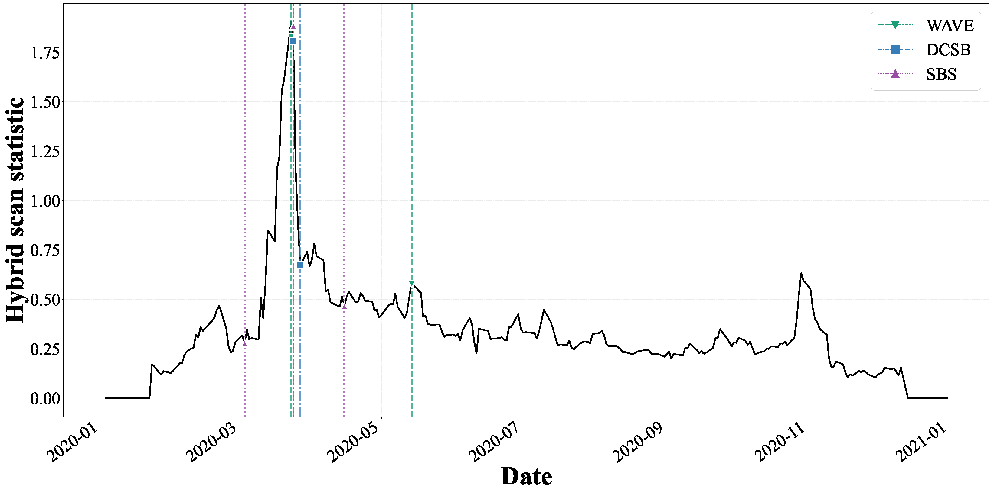
WAVE detects changes on 24 March and 14 May 2020. DCSB detects the 24 March change, whereas SBS detects changes on 3 March, 24 March, and 15 April. The 24 March date is therefore shared by all three procedures. It is close to the U.S. equity market trough on March 23 and to major Federal Reserve interventions during the COVID-19 market crisis [28]. The agreement across methods indicates that this episode contains strong multivariate evidence of a structural change. The additional SBS dates produce a finer segmentation of the highly volatile March and April period. The May 14 change detected by WAVE coincides with renewed uncertainty regarding the pace of economic recovery and the evolution of the pandemic [29].

The corresponding scan evidence is displayed in Figure 2. The vertical axis reports the hybrid scan statistic computed from the coordinatewise statistic defined in Equation (4). The dominant peak occurs during the March 2020 market crisis and coincides with the change identified by all three methods. A smaller but distinct increase is observed around the May detection, which supports the interpretation of an additional adjustment in the return process after the initial market collapse.

WAVE further provides coordinate-level attribution through its adaptive weights.

Table 6. Stocks with the largest WAVE adaptive weights. Larger weights indicate greater relative contribution to the weighted scan statistic.

Ticker	Company	Sector	Weight
DD	DuPont de Nemours, Inc.	Materials	0.0234
DOW	Dow Inc.	Materials	0.0191
F	Ford Motor Company	Consumer Discretionary	0.0189
AVGO	Broadcom Inc.	Information Technology	0.0173
GM	General Motors Company	Consumer Discretionary	0.0162
BA	The Boeing Company	Industrials	0.0162
AIG	American International Group, Inc.	Financials	0.0158
COP	ConocoPhillips	Energy	0.0157
NKE	NIKE, Inc.	Consumer Discretionary	0.0157
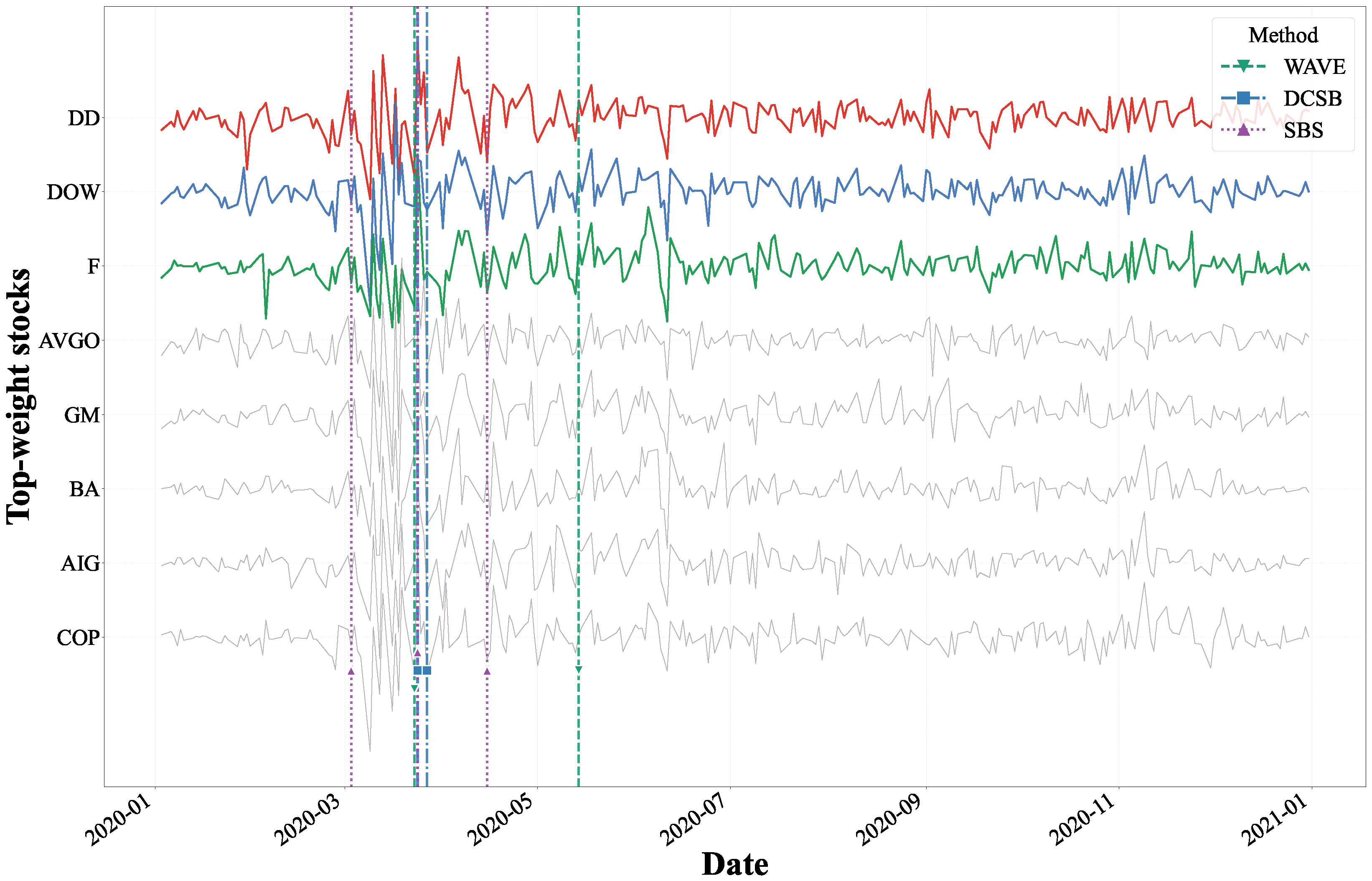
LOW	Lowe’s Companies, Inc.	Consumer Discretionary	0.0152

reports the stocks with the largest normalized weights, together with their company names and sectors, and Figure 3 displays their standardized return trajectories. Since the weights sum to one, they provide a relative ranking of coordinate-level contributions to the weighted scan statistic. The highest-ranked stocks are mainly from materials, consumer discretionary, industrials, financials, and energy, indicating that the detected changes are driven by sectors with strong exposure to the 2020 market disruption. These weights should be interpreted as statistical contribution measures rather than as causal effects of individual stocks.

This weight ranking is also consistent with the economic events surrounding the COVID-19 shock. Materials and industrial stocks were affected by weaker automotive and industrial demand, while automobile producers experienced production suspensions and subsequent restarts. Boeing was exposed to the collapse in air travel and disruptions in aircraft production, and energy stocks were affected by the sharp oil price decline in April 2020. Consumer discretionary firms were influenced by store closures, reopening dynamics, and changes in household demand, whereas financial firms were affected by equity market declines and changes in credit conditions. These events do not provide a true active set, but they support the interpretation that the largest WAVE weights are assigned to stocks whose return dynamics were plausibly sensitive to the major economic and market disruptions in 2020.

Taken together, the results show that all three methods identify the principal market disruption in March 2020, while their segmentations differ outside this dominant episode. Since the true structural changes are unknown, these differences do not establish that one set of dates is objectively correct. The empirical advantage of WAVE lies instead in the richness of its output. In addition to estimating change point locations, WAVE provides adaptive weights and active coordinate information that link each detected regime change to the stocks contributing the most strongly to the scan evidence. The application therefore illustrates how WAVE combines temporal localization with coordinate-level statistical attribution in a high-dimensional financial setting.

5. Conclusions

This paper proposes WAVE, a data-adaptive weighting framework for high-dimensional mean change point detection with coordinate-level attribution. By combining hybrid coordinatewise scan statistics, adaptive weighting, bootstrap calibration, recursive segmentation, and post-detection active coordinate identification, WAVE links change point localization with coordinate-level interpretation. The expanded simulations show accurate localization and informative support recovery in the settings considered, especially under moderate to strong signals, while support recovery becomes more challenging under weak signals, temporal dependence, or larger dimensions. The S&P 100 application further illustrates how the learned weights can help summarize coordinates associated with detected market regime changes. Several limitations should be noted. WAVE is developed under a working high-dimensional mean change framework. When applied directly to raw observations, it is not designed to detect pure variance changes or general distributional changes unless suitable transformations, such as centered squares or cross-products, are used. Heavy-tailed observations, nonstationary dependence, model misspecification, or abrupt changes in the error structure may also affect the coordinatewise scan statistics, adaptive weights, and bootstrap calibration. Robust preprocessing, dependence-aware calibration, and extensions to broader distributional changes are useful directions for future work.