Tsallis Entropy Measures for Concomitants of Generalized Order Statistics with Applications in Image Segmentation and Reliability Analysis

Abstract

This paper develops a general framework for Tsallis entropy (TsE) and cumulative residual Tsallis entropy (CRTsE) for concomitants of generalized order statistics under the Cambanis family of bivariate distributions. Explicit closed-form expressions and alternative representations for TsE and its cumulative residual counterparts, including a unique formulation of the alternative CRTsE, are derived. Various structural properties are established, including symmetry relations between low- and high-rank concomitants, as well as connections with classical submodels such as order statistics and record values. A nonparametric estimator for the CRTsE is proposed; its mean, variance, and consistency properties are investigated analytically and through extensive Monte Carlo simulations. The theoretical framework is further illustrated through two application domains: reliability assessment of real bivariate system data, and histogram-based image segmentation via a rank-sensitive Tsallis-thresholding scheme. The proposed methodology constitutes a flexible, dependence-aware generalization of classical Shannon-based entropy measures and is particularly advantageous for systems exhibiting nonlinear dependence, tail sensitivity, or non-extensive behavior.

1. Introduction

Multivariate statistical analysis, especially in the fields of information theory, reliability theory, and survival analysis, relies heavily on the modeling of dependence patterns between random variables (RVs). One classical approach that captures weak types of dependency in a basic yet analytically tractable model is the Farlie–Gumbel–Morgenstern (FGM) family of bivariate distributions. With the FGM family, which was first introduced by Farlie [1] and later expanded by Gumbel [2] and Morgenstern [3], positive and negative dependencies can be modeled with a single association parameter, and closed-form formulations for marginal and joint distributions can be preserved. But because the dependence parameter in the standard FGM model may only take values within a certain range, it cannot capture really strong dependencies. A number of broad statements have been put forth to overcome this restriction. Notable extensions include the Cambanis family (see [4,5]), which expands the FGM structure to include a broader class of copula-type functions (see [6]). These functions are able to better simulate a larger variety of dependencies, such as those in ranking data scenarios and dependability models. The distribution function (DF) of the Cambanis family, represented as CM$({\zeta }_1,{\zeta }_2)$, is expressed as follows:

$$C_{S,T}(s,t;\underline{\zeta })=C_S\left(s\right)C_T\left(t\right)\left[1+{\zeta }_1{\overline{C}}_T\left(t\right)+{\zeta }_2{\overline{C}}_S\left(s\right){\overline{C}}_T\left(t\right)\right],$$

(1)

where $C_S\left(s\right)$ and $C_T\left(t\right)$ are DFs of RVs S and $T,$ respectively, while ${\overline{C}}_S\left(s\right)=1-C_S\left(s\right)$ and ${\overline{C}}_T\left(t\right)=1-C_T\left(t\right)$ are the survivals functions (SFs) of S and $T,$ respectively. Here, we have the following probability density function (PDF):

$${\aleph }_{S,T}(s,t;\underline{\zeta })={\aleph }_S\left(s\right){\aleph }_T\left(t\right)\left[1+{\zeta }_1(1-2C_T\left(t\right)+{\zeta }_2(1-2C_S\left(s\right)(1-2C_T\left(t\right)\right],$$

(2)

where ${\aleph }_S\left(s\right)$ and ${\aleph }_T\left(t\right)$ are PDFs of S and $T,$ respectively. Cambanis [4] showed that the admissible parameter space is

$$\Theta =\left\{\zeta :1+{\zeta }_1+{\zeta }_2\ge 0;1-{\zeta }_1-{\zeta }_2\ge 0;1-{\zeta }_1+{\zeta }_2\ge 0;\right.\left.1+{\zeta }_1-{\zeta }_2\ge 0\right\}.$$

Several papers have studied this flexible model; see, for example, [7,8,9,10]. Information measurements are one of the key methods for addressing statistical modeling uncertainties and variability. This is notably true in reliability analysis, survival research, and image processing. However, differential entropy $H\left(S\right)$ is commonly utilized in dependability analysis, despite its well-known issues. It does not have a natural SF meaning and depends on the PDF, which may not exist or be hard to estimate. Rao et al. [11] introduced the cumulative residual entropy (CRE), a new uncertainty measure based on the SF of S:

$$\xi \left(S\right)=-{\int }_0^{\infty }{\overline{C}}_S\left(s\right)\log {\overline{C}}_S\left(s\right)ds,$$

The Boltzmann–Gibbs–Shannon formulation has long been used to estimate entropy, a key notion in thermodynamics, information theory, and statistical mechanics. On the other hand, reliable modeling using standard entropy is frequently not possible for complex systems that display features like multifractal structures, memory effects, or long-range interactions. Tsallis [12] proposed what is now called Tsallis entropy (TsE), a generalized entropy measure, to overcome these shortcomings. This measure is defined for the continuous RV S as

$$TsE\left(S\right)=\frac{1}{\tau -1}\left(1-{\int }_0^{\infty }{\left[{\aleph }_S\left(s\right)\right]}^{\tau }\right)ds,$$

(3)

where $0<\tau \ne 1,$ and if $\tau ⟶1,$ then $TsE\left(S\right)⟶H\left(S\right)$. Sati and Gupta [13] proposed the cumulative residual Tsallis entropy (CRTsE) of order $\tau$ (cf. [14]) as

$$\Psi \left(S\right)=\frac{1}{\tau -1}\left(1-{\int }_0^{\infty }{\left[{\overline{C}}_S\left(s\right)\right]}^{\tau }\right)ds,$$

(4)

when $\tau ⟶1,$ then $\Psi \left(S\right)⟶\xi \left(S\right).$ It is instructive to situate TsE within the broader landscape of generalized entropy measures. Rényi entropy of order $\tau$ is defined as $H_{\tau }^R\left(S\right)=\frac{1}{1-\tau }\log \int {\left[{\aleph }_S\left(s\right)\right]}^{\tau }\mathrm{d}s$. Both Rényi and Tsallis entropies share the same underlying functional $\int {\left[{\aleph }_S\left(s\right)\right]}^{\tau }\mathrm{d}s$; they are related by $\mathrm{TsE}\left(S\right)=\frac{1-\exp \left[(1-\tau )H_{\tau }^R\left(S\right)\right]}{\tau -1}$, so that for $\tau \ne 1$ the two measures carry equivalent information about the distribution. The appearance of a logarithm in the Rényi scale compresses the information and makes the measure additive for independent systems. This additivity is technically convenient but limits the flexibility of the model for complicated, dependent variables. On the contrary, the absence of the logarithm in the Tsallis formulation maintains a straight polynomial relation with the density kernel and so permits a simple non-additive structure. TsE is non-additive (or non-extensive) for independent systems, satisfying $\mathrm{TsE}(S,T)=\mathrm{TsE}\left(S\right)+\mathrm{TsE}\left(T\right)+(1-\tau )\mathrm{TsE}\left(S\right)\mathrm{TsE}\left(T\right)$, which makes it particularly advantageous for modeling systems with long-range dependence or power-law behavior properties that are relevant to the concomitant framework developed in this paper. Rajesh and Sunoj [15] introduced an alternative measure for CRTE (ACRTE) as follows:

$$\begin{array}{c}{\xi }_{\tau }\left(S\right)=\frac{1}{\tau -1}\left({\int }_0^{\infty }({\overline{C}}_S\left(s\right)-{\left[{\overline{C}}_S\left(s\right)\right]}^{\tau })ds\right),\eta >0,\eta \ne 1.\hfill \end{array}$$

(5)

Kamps [16] developed the generalized order statistics (GdOSs) model as an all-encompassing framework for ascendingly ordered RVs. The GdOSs model includes many important models of ordered RVs, as seen in Table 1. The RVs $S(r,n,\tilde{m},k),r=1,2,\dots ,n$ are called GdOS based on absolutely continuous DF $C_S$ with the PDF ${\aleph }_S,$ if their joint PDF (JPDF) has the form

$${\aleph }_{1,\dots ,n:n}^{(\tilde{m},k)}(s_1,\dots ,s_n)=\left({\displaystyle \prod _{j=1}^n}{\gamma }_j\right)\left({\displaystyle \prod _{j=1}^{n-1}}{\overline{C}}_S^{{\gamma }_j-{\gamma }_{j+1}-1}\left(s_j\right){\aleph }_S\left(s_j\right)\right){\overline{C}}_S^{{\gamma }_n-1}\left(s_n\right)f_S\left(s_n\right),$$

where $C^{-1}\left(0\right)\le s_1\le \dots \le s_n\le C^{-1}\left(1\right).$ The parameters ${\gamma }_1,\dots ,{\gamma }_n$ are defined by ${\gamma }_n=k>0,{\gamma }_r=k+n-r+{\sum }_{j=r}^{n-1}{m}_j,r=1,\dots ,n-1\mathrm{and}\tilde{m}=(m_1,m_2,\dots ,m_{n-1})\in \mathbb{R}$. The PDF of the rth GdOS is given by (cf. Kamps and Cramer [17])

$${\aleph }_{S(r,n,\tilde{m},k)}\left(s\right)={\eta }_{r-1}{\displaystyle \sum _{i=1}^r}{a}_i\left(r\right){\overline{C}}_S^{{\gamma }_i-1}\left(s\right){\aleph }_S\left(s\right),s\in \mathbb{R},1\le r\le n,$$

(6)

where ${\eta }_{r-1}={\displaystyle \prod _{i=1}^r}{\gamma }_i,a_i\left(r\right)={\displaystyle \prod _{\genfrac{}{}{0pt}{}{j=1}{j\ne i}}^r}\frac{1}{{\gamma }_j-{\gamma }_i},1\le i\le r\le n.$ Table 1 presents a unified view of several classical and generalized models as submodels within the versatile framework of GdOSs.

Table 1. Examples of submodels contained in the GdOS model.

${\mathit{m}}_{\mathit{j}},\mathit{j}\in \{1,\dots ,\mathit{n}-1\}$	$\mathit{k}(>0)$	${\mathit{\gamma }}_{\mathit{j}}(>0),\mathit{j}\in \{1,\dots ,\mathit{n}\}$	Model
0	1	$n-j+1$	Order statistics
0	$\alpha -n+1$	$\alpha -j+1$	Order statistics with nonintegral sample size
$m_j\in {\mathbb{N}}_0$	$k\in \mathbb{N}$	$n-j+k+{\sum }_{i=1}^{n-1}{m}_i$	Progressively type-II censored
m	k	$k+(n-j)(m+1)$	m-GdOSs
$(n-j+1){\alpha }_j$	${\alpha }_n$	$(n-j+1){\alpha }_j$	(Restricted) SOSs
$-(n-j){\alpha }_{j+1}-1$	1	1	Record values
$-1$	$k\in \mathbb{N}$	k	$k^{\mathrm{th}}$ Record values
${\alpha }_j-{\alpha }_{j+1}-1$	${\alpha }_n$	${\alpha }_j$	Pfeifer record values

The revived interest in concomitants may be attributed to their significance in selection processes and prediction problems. Yang [18] formulated the comprehensive theory of concomitants of order statistics (CTOSs). The topic has been studied by many researchers, see [7,8,19,20]. Let $(S_i,T_i),i=1,2,\dots ,n,$ be a random sample from a bivariate DF $C_{S,T}(s,t).$ The GdOSs of the S-variate that are associated with the GdOSs for the T sample are called concomitants of GdOSs (CGdOSs) and are denoted by $T_{[1,n,\tilde{m},k]},T_{[2,n,\tilde{m},k]},\dots ,T_{[n,n,\tilde{m},k]}$. The PDF of the concomitant of rth GdOS is given by (see [8,20])

$${\aleph }_{[r,n,\tilde{m},k]}\left(t\right)={\int }_0^{\infty }{\aleph }_{T|S}\left(t\right|s){\aleph }_{S(r,n,\tilde{m},k)}\left(s\right)ds,$$

(7)

where ${\aleph }_{T|S}\left(t\right|s)$ is the conditional PDF of T given $S.$ A broad investigation on Tsallis measures under CGdOS is presented in this paper, based on the CM$({\zeta }_1,{\zeta }_2)$.

The remainder of this paper is organized as follows. Section 2 introduces the framework of CGdOSs under the CM$({\zeta }_1,{\zeta }_2)$ family of bivariate distributions and derives the main results for TsE, including explicit representations and fundamental properties. Section 3 is devoted to the development of CRTsE and its alternative formulation, where several theoretical properties are established. Also, a nonparametric estimator is proposed, and its statistical characteristics, including mean and variance, are investigated with a comprehensive simulation study to evaluate the finite-sample performance of the proposed estimators under different parameter settings. Section 4 illustrates the practical applicability of the proposed methodology through real data analysis in terms of reliability and an image segmentation application based on TsE. Section 5 concludes the report with a summary and research proposals.

Motivation

The nonlinear dependence, tail phenomena, and higher-order interactions in modern data structures are much more complicated than the traditional practice in entropy measures. Independent frameworks are not practical in many applications, such as reliability engineering, survival analysis, and image processing, where observations are often dependent and presented in a sequential or ranked manner. The Shannon entropy and its cumulative residual counterpart have been widely used to quantify uncertainty, but these approaches may not provide enough flexibility to model systems with long-range dependence or non-extensive behavior. In this context, TsE provides a more flexible alternative, with an extra parameter that allows it to adjust its sensitivity to rare events and distribution tails. Simultaneously, CGdOSs offer a flexible toolset that provides a framework for dealing with dependent and ordered data generated by bivariate and multivariate models. Prompted by the necessity to combine structured dependence models with flexible entropy measures, this paper proposes a general framework for Tsallis-based uncertainty quantification in conjunction with at least one CGdOSs, particularly under the CM$({\zeta }_1,{\zeta }_2)$ family of distributions. This coupling between existing notions of entropy would not only generalize their properties but also allow them greater applicability in modeling complex systems found in nature. Over the past few years, entropy-based methods have continued to expand their presence in various aspects of image processing, including, but not limited to, change detection, target repair segmentation, automatic thresholding, and others; an area where uncertainty becomes fundamental for discriminating structures from noise. The classic Shannon-entropy-based approaches gained widespread use due to their simplicity and strong theoretical grounding, but tend to suffer from limited robustness to complex images (i.e., those with noise, low contrast, or heavy-tailed intensity distributions). For these cases, TsE is a better-suited, non-additive alternative with an adjustable parameter that allows fine-tuning of sensitivity to rare events and local intensity fluctuations. Due to its adjustable nature, TsE is widely used to enhance segmentation quality and retain image details, especially for rank-based or contextual thresholding techniques. The inclusion of TsE into statistical structures, such as the CGdOSs under various dependence-generating models, offers a promising path toward more precise image processing with knowledge of dependencies.

2. Tsallis Entropy for CGdOSs Based on CM$({\mathbf{\zeta }}_{\mathbf{1}},{\mathbf{\zeta }}_{\mathbf{2}})$ Family

In this section, we derive the CGdOS under the CM$({\zeta }_1,{\zeta }_2)$ family. Clear representations of well-known submodels within this category are provided to demonstrate the versatility and relevance of the proposed framework. The TsE is then articulated inside the framework of CGdOS, facilitating the quantification of uncertainty and information for dependent RVs dictated by the Cambanis structure.

Theorem 1. 

Let $T_{[r,n,\tilde{m},k]}$ represent CGdOSs from CM$({\zeta }_1,{\zeta }_2)$ family. Then, the PDF, CDF, and SF of $T_{[r,n,\tilde{m},k]}$ respectively are

$$\begin{array}{ccc}{\aleph }_{[r,n,\tilde{m},k]}\left(t\right)\hfill & =& {\aleph }_T\left(t\right)\left[1+{\zeta }_{(\tilde{m},k)}^{(r,n)}(1-2C_T\left(t\right))\right],\hfill \end{array}$$

(8)

$$\begin{array}{ccc}{C}_{[r,n,\tilde{m},k]}\left(t\right)\hfill & =& C_T\left(t\right)\left[1+{\zeta }_{(\tilde{m},k)}^{(r,n)}{\overline{C}}_T\left(t\right)\right],\hfill \end{array}$$

(9)

$$\begin{array}{ccc}{\overline{C}}_{[r,n,\tilde{m},k]}\left(t\right)\hfill & =& {\overline{C}}_T\left(t\right)\left[1-{\zeta }_{(\tilde{m},k)}^{(r,n)}{C}_T\left(t\right)\right],\hfill \end{array}$$

(10)

where ${\zeta }_{(\tilde{m},k)}^{(r,n)}={\zeta }_1+{\zeta }_2\left(2{\eta }_{r-1}{\sum }_{i=1}^r\frac{a_i\left(r\right)}{{\gamma }_i+1}-1\right),$${\eta }_{r-1}={\displaystyle \prod _{i=1}^r}{\gamma }_i, a_i\left(r\right)={\displaystyle \prod _{\genfrac{}{}{0pt}{}{j=1}{j\ne i}}^r}\frac{1}{{\gamma }_j-{\gamma }_i}, 1\le i\le r\le n.$

Proof. 

Based on (2), and (7), we then have

$$\begin{array}{ccc}{\aleph }_{[r,n,\tilde{m},k]}\left(t\right)\hfill & =& {\int }_0^{\infty }{\aleph }_{T|S}\left(t\right|s){\aleph }_{S(r,n,\tilde{m},k)}\left(s\right)ds\hfill \\ & =& {\int }_0^{\infty }{\aleph }_T\left(t\right)\left[1+{\zeta }_1(1-2C_T\left(t\right))+{\zeta }_2(1-2C_S\left(s\right))(1-2C_T\left(t\right))\right]\hfill \\ & \times & {\eta }_{r-1}{\displaystyle \sum _{i=1}^r}{a}_i\left(r\right){\overline{C}}_S^{{\gamma }_i-1}\left(s\right){\aleph }_S\left(s\right)ds\hfill \\ & =& {\eta }_{r-1}{\displaystyle \sum _{i=1}^r}{a}_i\left(r\right){\int }_{-\infty }^{\infty }{\aleph }_T\left(t\right)\left[1+(1-2C_T\left(t\right))({\zeta }_1+{\zeta }_2(1-2C_S\left(s\right)))\right]\hfill \\ & \times & {\overline{C}}_S^{{\gamma }_i-1}\left(s\right){\aleph }_S\left(s\right)ds\hfill \\ & =& {\aleph }_T\left(t\right)\left[1+{\zeta }_{(\tilde{m},k)}^{(r,n)}(1-2C_T\left(t\right))\right].\hfill \end{array}$$

where

$$\begin{array}{ccc}{\zeta }_{(\tilde{m},k)}^{(r,n)}\hfill & =& {\zeta }_1+{\zeta }_2{\eta }_{r-1}{\displaystyle \sum _{i=1}^r}{a}_i\left(r\right){\int }_0^{\infty }(2{\overline{C}}_S\left(s\right)-1){\overline{C}}_S^{{\gamma }_i-1}\left(s\right){\aleph }_S\left(s\right)ds\hfill \\ & =& {\zeta }_1+{\zeta }_2\left(2{\eta }_{r-1}{\displaystyle \sum _{i=1}^r}{a}_i\left(r\right){\int }_{-\infty }^{\infty }{\overline{C}}_S^{{\gamma }_i}{\aleph }_S\left(s\right)ds-1\right)\hfill \\ & =& {\zeta }_1+{\zeta }_2\left(2{\eta }_{r-1}{\displaystyle \sum _{i=1}^r}{a}_i\left(r\right){\int }_0^1{u}^{{\gamma }_i}du-1\right)\hfill \\ & =& {\zeta }_1+{\zeta }_2\left(2{\eta }_{r-1}{\displaystyle \sum _{i=1}^r}\frac{a_i\left(r\right)}{{\gamma }_i+1}-1\right).\hfill \end{array}$$

□

Three important subclasses of concomitants deserve special attention. First, when $\tilde{m}=0$ and $k=1$, we obtain the concomitants of order statistics (CTOSs) $T_{[r,n,0,1]}$. Second, when $\tilde{m}=-1$ and $k=1$, we obtain the concomitants of record values (ConRec) $T_{[n,-1,1]}^{\left(u\right)}$ (upper) and $T_{[n,-1,1]}^{\left(l\right)}$ (lower). Third, when all $m_j$ are equal to a constant m (with $m>-1$), we obtain the concomitants of m-generalized order statistics (m-GdOSs) $T_{[r,n,m,k]}$. Remark 1 below provides explicit density formulas for each of these three cases.

Remark 1. 

The framework of CGdOSs from the CM family provides a unified structure that encompasses several well-known models in statistical theory as special cases. Among the most prominent subclasses are the following:

1. 

Putting $\tilde{m}=0,$ $k=1,$ in ${\zeta }_{(\tilde{m},k)}^{(r,n)},$ we get the PDF of CTOSs based CM family as follows:

$${\aleph }_{[r,n,0,1]}\left(t\right)={\aleph }_T\left(t\right)\left[1+\left({\zeta }_1+{\zeta }_2(\frac{n-2r+1}{n+1})\right)(1-2C_T\left(t\right))\right].$$

2. 

Putting $\tilde{m}=-1,$ $k=1,$ in ${\zeta }_{(\tilde{m},k)}^{(r,n)},$ we get the PDFs of upper and lower ConRec, respectively, as follows:

$${\aleph }_{[n,-1,1]}^{\left(u\right)}\left(t\right)={\aleph }_T\left(t\right)[1+({\zeta }_1+{\zeta }_2(2^{-(n-1)}-1)\left)(1-2C_T\left(t\right))\right],$$

$${\aleph }_{[n,-1,1]}^{\left(l\right)}\left(t\right)={\aleph }_T\left(t\right)[1+({\zeta }_1+{\zeta }_2(1-2^{-(n-1)})\left)(1-2C_T\left(t\right))\right].$$

3. 

To get the m-GdOSs, taking $\tilde{m}=m.$ The PDF of concomitant of m-GdOSs based CM family is given by

$${\aleph }_{[r,n,m,k]}\left(t\right)={\aleph }_T\left(t\right)\left[1+\left({\zeta }_1+{\zeta }_2\left[2{\displaystyle \prod _{i=1}^r}\frac{{\gamma }_i}{{\gamma }_i+1}-1\right]\right)(1-2C_T\left(t\right))\right].$$

Theorem 2 (Quantile-based TsE).

For the CGdOS $T_{[r,n,\tilde{m},k]}$ from the $\mathrm{CM}({\zeta }_1,{\zeta }_2)$ family with $Q_T\left(u\right)=C_T^{-1}\left(u\right)$ and quantile density function $q_T\left(u\right)=Q_T^{\prime }\left(u\right)$. Then, the TsE of $T_{[r,n,\tilde{m},k]}$ is

$${\mathrm{TsE}}_{[r,n,\tilde{m},k]}=\frac{1}{\tau -1}\left\{1-{\mathbb{E}}_U\left[\frac{{\left[1+{\zeta }_{(\tilde{m},k)}^{(r,n)}(1-2U)\right]}^{\tau }}{{\left[q_T\left(U\right)\right]}^{\tau -1}}\right]\right\},$$

(11)

where $U\sim \mathrm{Uniform}(0,1)$, $0<\tau \ne 1$, and

$${\zeta }_{(\tilde{m},k)}^{(r,n)}={\zeta }_1+{\zeta }_2\left(2{\eta }_{r-1}{\displaystyle \sum _{i=1}^r}\frac{a_i\left(r\right)}{{\gamma }_i+1}-1\right).$$

Proof. 

From the TsE definition (3) and the PDF of the CGdOS (8), we obtain

$${\mathrm{TsE}}_{[r,n,\tilde{m},k]}=\frac{1}{\tau -1}\left\{1-{\int }_0^{\infty }{\left[{\aleph }_T\left(t\right)\left(1+{\zeta }_{(\tilde{m},k)}^{(r,n)}\left(1-2C_T\left(t\right)\right)\right)\right]}^{\tau }\mathrm{d}t\right\}.$$

Setting $u=C_T\left(t\right)$, we have $\mathrm{d}t=q_T\left(u\right)\mathrm{d}u$. Hence,

$$\begin{array}{cc}\hfill & {\left[{\aleph }_T\left(t\right)\left(1+{\zeta }_{(\tilde{m},k)}^{(r,n)}\left(1-2C_T\left(t\right)\right)\right)\right]}^{\tau }\mathrm{d}t\hfill \\ \hfill & ={\left[{\aleph }_T\left(Q_T\left(u\right)\right)\right]}^{\tau }{\left[1+{\zeta }_{(\tilde{m},k)}^{(r,n)}(1-2u)\right]}^{\tau }{q}_T\left(u\right)\mathrm{d}u\hfill \\ \hfill & =\frac{{\left[1+{\zeta }_{(\tilde{m},k)}^{(r,n)}(1-2u)\right]}^{\tau }}{q_T{\left(u\right)}^{\tau -1}}\mathrm{d}u.\hfill \end{array}$$

Substituting into the integral and recognizing the expectation with respect to $U\sim \mathrm{Uniform}(0,1)$ completes the proof.    □

Lemma 1. 

For any $({\zeta }_1,{\zeta }_2)\in \Theta$ and $u\in [0,1]$,

$$-1\le {\zeta }_{(\tilde{m},k)}^{(r,n)}(1-2u)\le 1,$$

so that $1+{\zeta }_{(\tilde{m},k)}^{(r,n)}(1-2u)\ge 0$ for all $u\in [0,1]$.

Proof. 

From $\Theta$, we have $|{\zeta }_1+{\zeta }_2|\le 1$ and $|{\zeta }_1-{\zeta }_2|\le 1$. Since $\lambda :={\eta }_{r-1}{\sum }_{i=1}^r\frac{a_i\left(r\right)}{{\gamma }_i+1}\in [0,1]$, we can write

$${\zeta }_{(\tilde{m},k)}^{(r,n)}=\lambda ({\zeta }_1+{\zeta }_2)+(1-\lambda )({\zeta }_1-{\zeta }_2)\in [-1,1].$$

For $u\in [0,1]$, $|1-2u|\le 1$, so $|{\zeta }_{(\tilde{m},k)}^{(r,n)}(1-2u)|\le 1$. Adding 1 gives the result.    □

Theorem 3 (Another representation of TsE).

Let $T_{[r,n,\tilde{m},k]}$ be the CGdOSs from CM$({\zeta }_1,{\zeta }_2)$ family. Then the TsE of $T_{[r,n,\tilde{m},k]}$

$${\mathrm{TsE}}_{[r,n,\tilde{m},k]}=\frac{1}{\tau -1}\left\{1-{\displaystyle \sum _{i=0}^{\mathcal{N}\left(\tau \right)}}\left(\genfrac{}{}{0pt}{}{\mathcal{N}\left(\tau \right)}{i}\right){\left[{\zeta }_{(\tilde{m},k)}^{(r,n)}\right]}^i{\mathbb{E}}_U\left[\frac{{(1-2U)}^i}{{\left(q_T\left(U\right)\right)}^{\tau -1}}\right]\right\},$$

(12)

where $N\left(\tau \right)=\tau$ if $\tau \in {\mathbb{Z}}^{+}$ and $N\left(\tau \right)=\infty$ otherwise.

Proof. 

Based on (8) and (3), we then have

$$\begin{array}{ccc}Ts{E}_{[r,n,\tilde{m},k]}\left(t\right)\hfill & =& \frac{1}{\tau -1}\left(1-{\int }_0^{\infty }{\left[{\aleph }_{[r,n,\tilde{m},k]}\left(t\right)\right]}^{\tau }dt\right)\hfill \\ & =& \frac{1}{\tau -1}\left(1-{\int }_0^{\infty }{\left[{\aleph }_T\left(t\right)\left[1+{\zeta }_{(\tilde{m},k)}^{(r,n)}(1-2C_T\left(t\right))\right]\right]}^{\tau }dt\right).\hfill \end{array}$$

Expanding ${(1+{\zeta }_{(\tilde{m},k)}^{(r,n)}(1-2C_T\left(t\right)))}^{\tau }$ via the generalized binomial. Then,

$$\begin{array}{ccc}Ts{E}_{[r,n,\tilde{m},k]}\left(t\right)\hfill & =& \frac{1}{\tau -1}\left(1-{\displaystyle \sum _{i=0}^{\mathcal{N}\left(\tau \right)}}\left(\genfrac{}{}{0pt}{}{\mathcal{N}\left(\tau \right)}{i}\right){\left[{\zeta }_{(\tilde{m},k)}^{(r,n)}\right]}^i{\int }_0^{\infty }\left[{\aleph }_T{\left(t\right)}^{\tau }{(1-2C_T\left(t\right))}^i\right]dt\right).\hfill \end{array}$$

After taking $C_T\left(t\right)=u.$, we then have

$$\begin{array}{ccc}Ts{E}_{[r,n,\tilde{m},k]}\left(t\right)\hfill & =& \frac{1}{\tau -1}\left(1-{\displaystyle \sum _{i=0}^{\mathcal{N}\left(\tau \right)}}\left(\genfrac{}{}{0pt}{}{\mathcal{N}\left(\tau \right)}{i}\right){\left[{\zeta }_{(\tilde{m},k)}^{(r,n)}\right]}^i{\int }_0^1\left[{\aleph }_T{\left(C^{-1}\left(u\right)\right)}^{\tau -1}{(1-2u)}^i\right]du\right).\hfill \end{array}$$

Recognizing the integral as an expectation with respect to $U\sim \mathrm{Uniform}(0,1)$ completes the proof.    □

Theorem 4. 

Let $\tau >0$ with $\tau \notin {\mathbb{Z}}^{+}$, and let $({\zeta }_1,{\zeta }_2)\in \Theta$. For $u\in [0,1]$, define $z\left(u\right)={\zeta }_{(\tilde{m},k)}^{(r,n)}(1-2u)$. Then for every $u\in [0,1]$,

$${(1+z\left(u\right))}^{\tau }={\displaystyle \sum _{i=0}^{\infty }}\left(\genfrac{}{}{0pt}{}{\tau }{i}\right){\left[{\zeta }_{(\tilde{m},k)}^{(r,n)}\right]}^i{(1-2u)}^i,$$

where the series converges absolutely for $u\in (0,1)$ and conditionally for $u\in \{0,1\}$ when $|{\zeta }_{(\tilde{m},k)}^{(r,n)}|=1$; if $\tau \in {\mathbb{Z}}^{+}$, the series terminates at $i=\tau$. Moreover, if the marginal distribution satisfies the condition

$${\mathcal{I}}_{\tau }:={\mathbb{E}}_U\left[\frac{1}{q_T{\left(U\right)}^{\tau -1}}\right]={\int }_0^1\frac{du}{q_T{\left(u\right)}^{\tau -1}}<\infty ,$$

then the expectation in Theorem 3 is finite and the interchange of sum and integral is justified.

Proof. 

By Lemma 1, $|{\zeta }_{(\tilde{m},k)}^{(r,n)}|\le 1$ and $|1-2u|\le 1$, hence $\left|z\right(u\left)\right|\le 1$. For $u\in (0,1)$ we have $\left|z\right(u\left)\right|<1$; the binomial series then converges absolutely because $\left(\genfrac{}{}{0pt}{}{\tau }{i}\right)\sim C/i^{\tau +1}$ and $\sum i^{-(\tau +1)}<\infty$ for $\tau >0$. For $u=0$ or $u=1$, if $\left|\zeta \right|<1$ absolute convergence holds as before, and if $\left|\zeta \right|=1$ then $z\left(u\right)=\pm 1$ and $\left(\genfrac{}{}{0pt}{}{\tau }{i}\right)\sim {(-1)}^{i+1}\tau /i^{\tau +1}$; the alternating series test gives conditional convergence, and Abel’s theorem ensures the sum equals ${(1\pm 1)}^{\tau }$. If $\tau \in {\mathbb{Z}}^{+}$, then $\left(\genfrac{}{}{0pt}{}{\tau }{i}\right)=0$ for $i>\tau$, so the series terminates. Finally, since ${|1-2U|}^i\le 1$, we have ${|(1-2U)}^i/q_T{\left(U\right)}^{\tau -1}|\le 1/q_T{\left(U\right)}^{\tau -1}$. The condition ${\mathcal{I}}_{\tau }<\infty$ guarantees integrability, and the dominated convergence theorem justifies the interchange of sum and expectation in Theorem 3.    □

Remark 2. 

The interchange of summation and integration in the proof of Theorem 3 is justified as follows. By Lemma 1, $|1+{\zeta }_{(\tilde{m},k)}^{(r,n)}(1-2u)|\le 2$ uniformly in u. Hence, each partial sum of the binomial expansion is bounded by $2^{\tau }{\left[{\aleph }_T\left(C_T^{-1}\left(u\right)\right)\right]}^{\tau }$ uniformly in u, and the integrability condition $I_{\tau }<\infty$ provides a dominating integrable function.

Proposition 1. 

For the CTOSs $T_{[r,n,0,1]}.$ Then

$$\begin{array}{ccc}Ts{E}_{[r,n,0,1]}(t;{\zeta }_1,{\zeta }_2)\hfill & =& Ts{E}_{[n-r+1,n,0,1]}(t;{\zeta }_1,-{\zeta }_2)\hfill \end{array}$$

(13)

Proof. 

Based on item 1 in Remark 1, and (3), we then have

$$\begin{array}{ccc}T{E}_{[n-r+1,n,0,1]}(t;{\zeta }_1,-{\zeta }_2)\hfill & =& \frac{1}{\tau -1}\left(1-{\int }_0^{\infty }{\left[{\aleph }_T\left(t\right)\left[1+\left({\zeta }_1-{\zeta }_2\left(\frac{n-2(n-r+1)+1}{n+1}\right)\right)(1-2C_T\left(t\right))\right]\right]}^{\tau }dt\right)\hfill \\ & =& \frac{1}{\tau -1}\left(1-{\int }_0^{\infty }{\left[{\aleph }_T\left(t\right)\left[1+\left({\zeta }_1+{\zeta }_2\left(\frac{n-2r+1}{n+1}\right)\right)(1-2C_T\left(t\right))\right]\right]}^{\tau }dt\right).\hfill \\ & =& Ts{E}_{[r,n,0,1]}(t;{\zeta }_1,{\zeta }_2).\hfill \end{array}$$

   □

Proposition 2. 

For the ConRec $T_{[r,n,-1,1]}$. Then

$$\begin{array}{ccc}Ts{E}_{[n,-1,1]}^{\left(u\right)}(t;{\zeta }_1,{\zeta }_2)\hfill & =& Ts{E}_{[n,-1,1]}^{\left(l\right)}(t;{\zeta }_1,-{\zeta }_2).\hfill \end{array}$$

(14)

Proof. 

According to item 2 in Remark 1, we have

$$\begin{array}{ccc}Ts{E}_{[n,-1,1]}^{\left(u\right)}(t;{\zeta }_1,{\zeta }_2)\hfill & =& \frac{1}{\tau -1}\left(1-{\int }_0^{\infty }{\left[{\aleph }_T\left(t\right)\left[1+\left({\zeta }_1+{\zeta }_2(2^{-(n-1)}-1)\right)(1-2C_T\left(t\right))\right]\right]}^{\tau }dt\right)\hfill \\ & =& \frac{1}{\tau -1}\left(1-{\int }_0^{\infty }{\left[{\aleph }_T\left(t\right)\left[1+\left({\zeta }_1-{\zeta }_2(1-2^{-(n-1)})\right)(1-2C_T\left(t\right))\right]\right]}^{\tau }dt\right)\hfill \\ & =& Ts{E}_{[n,-1,1]}^{\left(l\right)}(t;{\zeta }_1,-{\zeta }_2).\hfill \end{array}$$

□

Example 1. 

Let S and T be exponentially distributed (CM-ED) RVs with bivariate DF:

$$\begin{array}{ccc}{C}_{S,T}(s,t;\underline{\zeta })\hfill & =& (1-\exp \left(\frac{-s}{{\theta }_1}\right))(1-\exp \left(\frac{-t}{{\theta }_2}\right))\left[1+{\zeta }_1\exp \left(\frac{-t}{{\theta }_2}\right)\right.\hfill \\ & +& \left.{\zeta }_2\exp \left(\frac{-s}{{\theta }_1}\right)\exp \left(\frac{-t}{{\theta }_2}\right)\right],s,t,{\theta }_1,{\theta }_2>0.\hfill \end{array}$$

From (12), we get n the TsE of $T_{[r,n,\tilde{m},k]}$ as follows:

$$\begin{array}{ccc}Ts{E}_{[r,n,\tilde{m},k]}\left(t\right)\hfill & =& \frac{1}{\tau -1}\left(1-{\displaystyle \sum _{i=0}^{\mathcal{N}\left(\tau \right)}}{\displaystyle \sum _{j=0}^i}\left(\genfrac{}{}{0pt}{}{\mathcal{N}\left(\tau \right)}{i}\right)\left(\genfrac{}{}{0pt}{}{i}{j}\right){(-2)}^j{\left[{\zeta }_{(\tilde{m},k)}^{(r,n)}\right]}^i{\theta }_2^{1-\tau }\beta \left(j+1,\tau \right)\right).\hfill \end{array}$$

(15)

Example 2. 

Let S and T be uniformly distributed from CM family (CM-UD) RVs with bivariate DF:

$$\begin{gathered} C_{S,T}(s,t)=\frac{st}{{\theta }_1{\theta }_2}\left[1+{\zeta }_1\left(1-\frac{t}{{\theta }_2}\right)+{\zeta }_2\left(1-\frac{s}{{\theta }_1}\right)\left(1-\frac{t}{{\theta }_2}\right)\right], \\ 0<s<{\theta }_1,0<t<{\theta }_2. \end{gathered}$$

The TsE of $T_{[r,n,\tilde{m},k]}$ based on CM-UD family is

$$Ts{E}_{[r,n,\tilde{m},k]}=\frac{1}{\tau -1}\left\{1-{\displaystyle \sum _{i=0}^{\mathcal{N}\left(\tau \right)}}\left(\genfrac{}{}{0pt}{}{\mathcal{N}\left(\tau \right)}{i}\right){\zeta }^i\frac{{(-1)}^i+1}{{\theta }_2^{\tau -1}2(i+1)}\right\}.$$

(16)

Example 3. 

Let the DF bivariate CM Weibull distribution (CM-WD) be

$$\begin{gathered} C_{S,T}(s,t)=(1-e^{-{\left(\frac{s}{{\theta }_1}\right)}^{{\beta }_1}})(1-e^{-{\left(\frac{s}{{\theta }_2}\right)}^{{\beta }_2}})[1+{\zeta }_1(e^{-{\left(\frac{t}{{\theta }_2}\right)}^{{\beta }_2}})+{\zeta }_2(e^{-{\left(\frac{s}{{\theta }_1}\right)}^{{\beta }_1}}\left)\right(e^{-{\left(\frac{t}{{\theta }_2}\right)}^{{\beta }_2}}\left)\right], \\ 0<s,t,{\theta }_1,{\theta }_2,{\beta }_1,{\beta }_2. \end{gathered}$$

The TsE of $T_{[r,n,\tilde{m},k]}$ based on CM-WD family is

$$\begin{array}{cc}Ts{E}_{[r,n,\tilde{m},k]}\hfill & =\frac{1}{\tau -1}\{1-{\displaystyle \sum _{i=0}^{\mathcal{N}\left(\tau \right)}}{\displaystyle \sum _{j=0}^i}{\displaystyle \sum _{k=0}^j}\left(\genfrac{}{}{0pt}{}{\mathcal{N}\left(\tau \right)}{i}\right)\left(\genfrac{}{}{0pt}{}{i}{j}\right)\left(\genfrac{}{}{0pt}{}{j}{k}\right){(-1)}^k{(-2)}^j{\zeta }^i\hfill \\ \hfill & \times {\beta }_2^{\tau -1}{\theta }_2^{-(\tau -1)}\Gamma \left(\frac{({\beta }_2-1)\tau +1}{{\beta }_2}\right){(\tau +k)}^{-({\beta }_2\tau -\tau +1)/{\beta }_2}\}.\hfill \end{array}$$

(17)

The TsE behavior under CM-ED for various dependent structures of data is shown in Figure 1 and Figure 2, and is based on CTOS and ConRec. TsE decreases monotonically, demonstrating the reaction of entropy to $\tau$. Higher r values and dependency parameters (${\zeta }_1,{\zeta }_2$) lead to greater initial TsE values. CTOS assembles these values more quickly than ConRec. As seen in Figure 2, TsE for upper contemporaneous record values is more sensitive to parameter changes, leading to a larger spread in the curves. Higher-entropy scenarios for various dependent data structures and CM-ED predictive capabilities are also supported by different results. Table 2 and Table 3 are for CTOS TsE, with distinct considerations for how data is allocated, along with their respective parameters. Table 2 shows that TsE increases with r when ${\zeta }_2>0$. The sign ${\zeta }_2<0$ means that TsE decreases with r. For negative values of ${\zeta }_2$, TsE is positively correlated with rank at lower ranks and negatively correlated with rank at higher ranks. The converse is true when ${\zeta }_2$ is positive. As shown by Table 3, for uniform distributions, TsE has nice symmetry at $r=n/2$ thanks to the fact that its entropy values are a constant at the median order statistic with respect to permutations. In contrast, the effect of ${\zeta }_2$ is even less impactful than that induced by the exponential scenario, such that variations in ${\zeta }_2$ primarily influence limits ($r=1$ and $r=n$). Deduced properties and relationships:

• $Ts{E}_{[r,n,0,1]}(t;{\zeta }_1,{\zeta }_2)=Ts{E}_{[n-r+1,n,0,1]}(t;{\zeta }_1,-{\zeta }_2)$
• The exponential case is sensitive to extreme values, leading to sharper variations in $TsE$, while the uniform case exhibits smoother behavior due to its bounded support.
• For fixed n, $TsE$ achieves its maximum at central ranks and minimum at the extremes ($r=1$ and $r=n$) in CM-UD.

Figure 1. TsE behavior in CTOSs under CM-ED at $n=20$.

Figure 1. TsE behavior in CTOSs under CM-ED at $n=20$.

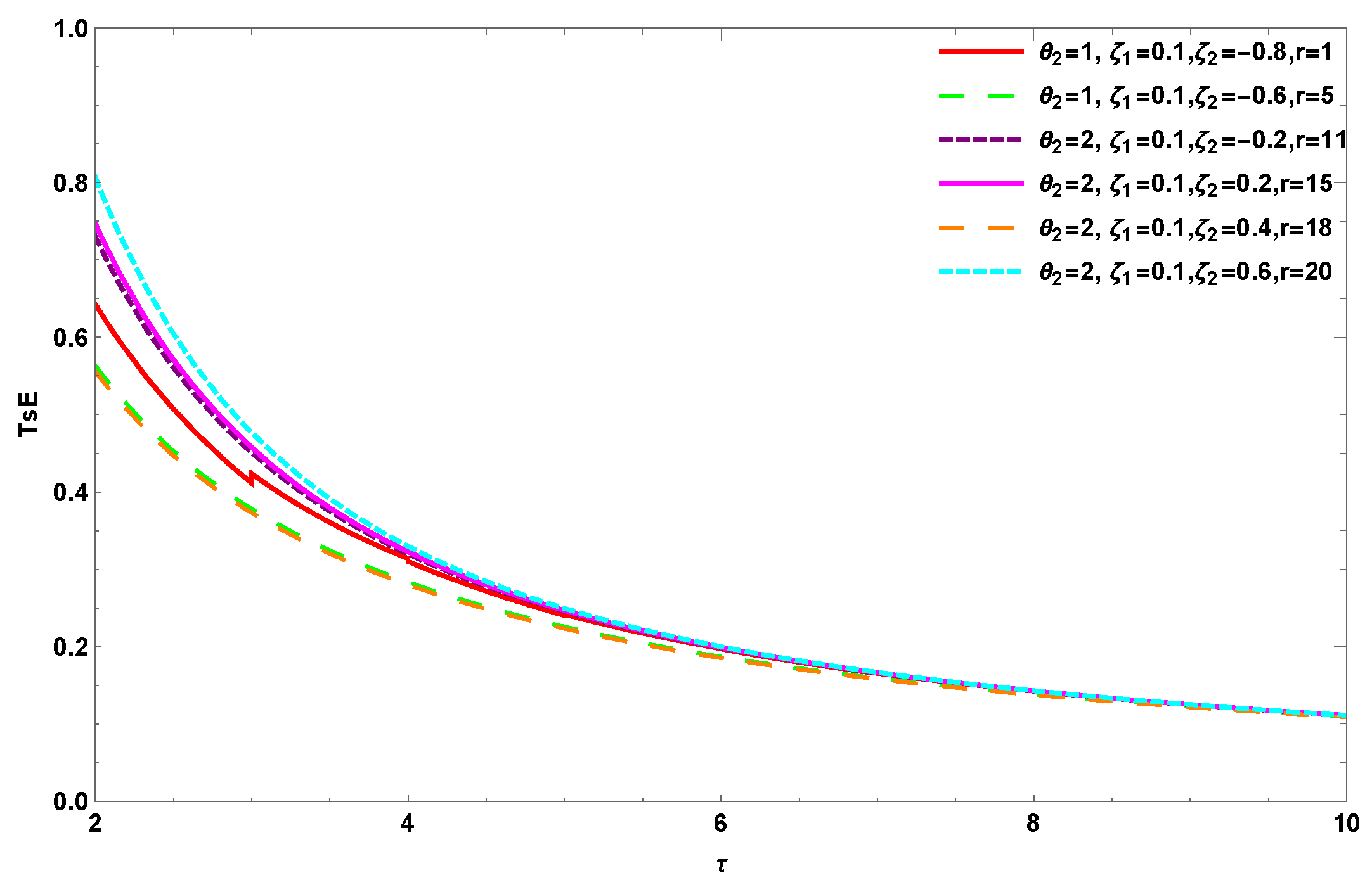
Figure 2. $TsE$ in upper ConRec-based CM-ED.

Figure 2. $TsE$ in upper ConRec-based CM-ED.

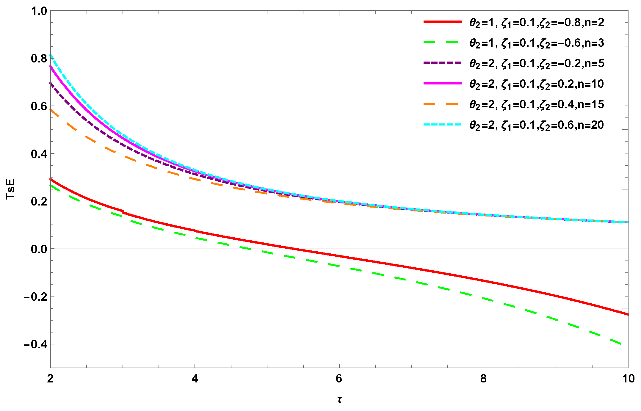
Table 2. $Ts{E}_{[r,n,0,1]}(t;{\zeta }_1,{\zeta }_2)$ for the CM-ED.

${\mathit{\theta }}_2=1,\mathit{\tau }=4,{\mathit{\zeta }}_1=0.1$
$\mathit{n}$	$\mathit{r}$	${\mathit{\zeta }}_{\mathbf{2}}=-\mathbf{0.8}$	${\mathit{\zeta }}_{\mathbf{2}}=-\mathbf{0.6}$	${\mathit{\zeta }}_{\mathbf{2}}=-\mathbf{0.4}$	${\mathit{\zeta }}_{\mathbf{2}}=-\mathbf{0.2}$	${\mathit{\zeta }}_{\mathbf{2}}=\mathbf{0.2}$	${\mathbf{\zeta }}_{\mathbf{2}}=\mathbf{0.4}$	${\mathbf{\zeta }}_{\mathbf{2}}=\mathbf{0.6}$	${\mathbf{\zeta }}_{\mathbf{2}}=\mathbf{0.8}$
5	1	0.3020	0.2921	0.2774	0.2564	0.1890	0.1387	0.0746	−0.0059
5	2	0.2774	0.2678	0.2564	0.2431	0.2096	0.1890	0.1654	0.1387
5	3	0.2275	0.2275	0.2275	0.2275	0.2275	0.2275	0.2275	0.2275
5	4	0.1387	0.1654	0.1890	0.2096	0.2431	0.2564	0.2678	0.2774
5	5	−0.0059	0.0746	0.1387	0.1890	0.2564	0.2774	0.2921	0.3020
10	1	0.3078	0.2993	0.2848	0.2618	0.1787	0.1114	0.0216	−0.0954
10	2	0.3005	0.2904	0.2758	0.2553	0.1910	0.1438	0.0842	0.0100
10	3	0.2887	0.2782	0.2649	0.2482	0.2024	0.1722	0.1361	0.0936
10	4	0.2706	0.2618	0.2518	0.2404	0.2130	0.1968	0.1787	0.1585
10	5	0.2444	0.2404	0.2363	0.2320	0.2229	0.2181	0.2130	0.2078
10	6	0.2078	0.2130	0.2181	0.2229	0.2320	0.2363	0.2404	0.2444
10	7	0.1585	0.1787	0.1968	0.2130	0.2404	0.2518	0.2618	0.2706
10	8	0.0936	0.1361	0.1722	0.2024	0.2482	0.2649	0.2782	0.2887
10	9	0.0100	0.0842	0.1438	0.1910	0.2553	0.2758	0.2904	0.3005
10	10	−0.0954	0.0216	0.1114	0.1787	0.2618	0.2848	0.2993	0.3078
19	1	0.3099	0.3024	0.2883	0.2646	0.1728	0.0954	−0.0104	−0.1510
19	2	0.3072	0.2986	0.2840	0.2612	0.1799	0.1149	0.0284	−0.0838
19	3	0.3035	0.2939	0.2791	0.2576	0.1868	0.1330	0.0636	−0.0242
19	4	0.2986	0.2883	0.2738	0.2539	0.1933	0.1498	0.0954	0.0284
19	5	0.2921	0.2816	0.2678	0.2500	0.1996	0.1654	0.1241	0.0746
19	6	0.2840	0.2738	0.2612	0.2459	0.2057	0.1799	0.1498	0.1149
19	7	0.2738	0.2646	0.2539	0.2416	0.2115	0.1933	0.1728	0.1498
19	8	0.2612	0.2539	0.2459	0.2371	0.2171	0.2057	0.1933	0.1799
19	9	0.2459	0.2416	0.2371	0.2324	0.2224	0.2171	0.2115	0.2057
19	10	0.2275	0.2275	0.2275	0.2275	0.2275	0.2275	0.2275	0.2275
19	11	0.2057	0.2115	0.2171	0.2224	0.2324	0.2371	0.2416	0.2459
19	12	0.1799	0.1933	0.2057	0.2171	0.2371	0.2459	0.2539	0.2612
19	13	0.1498	0.1728	0.1933	0.2115	0.2416	0.2539	0.2646	0.2738
19	14	0.1149	0.1498	0.1799	0.2057	0.2459	0.2612	0.2738	0.2840
19	15	0.0746	0.1241	0.1654	0.1996	0.2500	0.2678	0.2816	0.2921
19	16	0.0284	0.0954	0.1498	0.1933	0.2539	0.2738	0.2883	0.2986
19	17	−0.0242	0.0636	0.1330	0.1868	0.2576	0.2791	0.2939	0.3035
19	18	−0.0838	0.0284	0.1149	0.1799	0.2612	0.2840	0.2986	0.3072
19	19	−0.1510	−0.0104	0.0954	0.1728	0.2646	0.2883	0.3024	0.3099

Table 2. $Ts{E}_{[r,n,0,1]}(t;{\zeta }_1,{\zeta }_2)$ for the CM-ED.

${\mathit{\theta }}_2=1,\mathit{\tau }=4,{\mathit{\zeta }}_1=0.1$
$\mathit{n}$	$\mathit{r}$	${\mathit{\zeta }}_{\mathbf{2}}=-\mathbf{0.8}$	${\mathit{\zeta }}_{\mathbf{2}}=-\mathbf{0.6}$	${\mathit{\zeta }}_{\mathbf{2}}=-\mathbf{0.4}$	${\mathit{\zeta }}_{\mathbf{2}}=-\mathbf{0.2}$	${\mathit{\zeta }}_{\mathbf{2}}=\mathbf{0.2}$	${\mathbf{\zeta }}_{\mathbf{2}}=\mathbf{0.4}$	${\mathbf{\zeta }}_{\mathbf{2}}=\mathbf{0.6}$	${\mathbf{\zeta }}_{\mathbf{2}}=\mathbf{0.8}$
5	1	0.3020	0.2921	0.2774	0.2564	0.1890	0.1387	0.0746	−0.0059
5	2	0.2774	0.2678	0.2564	0.2431	0.2096	0.1890	0.1654	0.1387
5	3	0.2275	0.2275	0.2275	0.2275	0.2275	0.2275	0.2275	0.2275
5	4	0.1387	0.1654	0.1890	0.2096	0.2431	0.2564	0.2678	0.2774
5	5	−0.0059	0.0746	0.1387	0.1890	0.2564	0.2774	0.2921	0.3020
10	1	0.3078	0.2993	0.2848	0.2618	0.1787	0.1114	0.0216	−0.0954
10	2	0.3005	0.2904	0.2758	0.2553	0.1910	0.1438	0.0842	0.0100
10	3	0.2887	0.2782	0.2649	0.2482	0.2024	0.1722	0.1361	0.0936
10	4	0.2706	0.2618	0.2518	0.2404	0.2130	0.1968	0.1787	0.1585
10	5	0.2444	0.2404	0.2363	0.2320	0.2229	0.2181	0.2130	0.2078
10	6	0.2078	0.2130	0.2181	0.2229	0.2320	0.2363	0.2404	0.2444
10	7	0.1585	0.1787	0.1968	0.2130	0.2404	0.2518	0.2618	0.2706
10	8	0.0936	0.1361	0.1722	0.2024	0.2482	0.2649	0.2782	0.2887
10	9	0.0100	0.0842	0.1438	0.1910	0.2553	0.2758	0.2904	0.3005
10	10	−0.0954	0.0216	0.1114	0.1787	0.2618	0.2848	0.2993	0.3078
19	1	0.3099	0.3024	0.2883	0.2646	0.1728	0.0954	−0.0104	−0.1510
19	2	0.3072	0.2986	0.2840	0.2612	0.1799	0.1149	0.0284	−0.0838
19	3	0.3035	0.2939	0.2791	0.2576	0.1868	0.1330	0.0636	−0.0242
19	4	0.2986	0.2883	0.2738	0.2539	0.1933	0.1498	0.0954	0.0284
19	5	0.2921	0.2816	0.2678	0.2500	0.1996	0.1654	0.1241	0.0746
19	6	0.2840	0.2738	0.2612	0.2459	0.2057	0.1799	0.1498	0.1149
19	7	0.2738	0.2646	0.2539	0.2416	0.2115	0.1933	0.1728	0.1498
19	8	0.2612	0.2539	0.2459	0.2371	0.2171	0.2057	0.1933	0.1799
19	9	0.2459	0.2416	0.2371	0.2324	0.2224	0.2171	0.2115	0.2057
19	10	0.2275	0.2275	0.2275	0.2275	0.2275	0.2275	0.2275	0.2275
19	11	0.2057	0.2115	0.2171	0.2224	0.2324	0.2371	0.2416	0.2459
19	12	0.1799	0.1933	0.2057	0.2171	0.2371	0.2459	0.2539	0.2612
19	13	0.1498	0.1728	0.1933	0.2115	0.2416	0.2539	0.2646	0.2738
19	14	0.1149	0.1498	0.1799	0.2057	0.2459	0.2612	0.2738	0.2840
19	15	0.0746	0.1241	0.1654	0.1996	0.2500	0.2678	0.2816	0.2921
19	16	0.0284	0.0954	0.1498	0.1933	0.2539	0.2738	0.2883	0.2986
19	17	−0.0242	0.0636	0.1330	0.1868	0.2576	0.2791	0.2939	0.3035
19	18	−0.0838	0.0284	0.1149	0.1799	0.2612	0.2840	0.2986	0.3072
19	19	−0.1510	−0.0104	0.0954	0.1728	0.2646	0.2883	0.3024	0.3099

Table 3. $Ts{E}_{[r,n,0,1]}(t;{\zeta }_1,{\zeta }_2)$ for the CM-UD.

${\mathit{\theta }}_2=2,\mathit{\tau }=4,{\mathit{\zeta }}_1=0.1$
$\mathit{n}$	$\mathit{r}$	${\mathit{\zeta }}_{\mathbf{2}}=-\mathbf{0.8}$	${\mathit{\zeta }}_{\mathbf{2}}=-\mathbf{0.6}$	${\mathit{\zeta }}_{\mathbf{2}}=-\mathbf{0.4}$	${\mathit{\zeta }}_{\mathbf{2}}=-\mathbf{0.2}$	${\mathit{\zeta }}_{\mathbf{2}}=\mathbf{0.2}$	${\mathit{\zeta }}_{\mathbf{2}}=\mathbf{0.4}$	${\mathit{\zeta }}_{\mathbf{2}}=\mathbf{0.6}$	${\mathit{\zeta }}_{\mathbf{2}}=\mathbf{0.8}$
5	1	0.2757	0.2841	0.2893	0.2916	0.2871	0.2803	0.2703	0.2569
5	2	0.2893	0.2908	0.2916	0.2916	0.2893	0.2871	0.2841	0.2803
5	3	0.2908	0.2908	0.2908	0.2908	0.2908	0.2908	0.2908	0.2908
5	4	0.2803	0.2841	0.2871	0.2893	0.2916	0.2916	0.2908	0.2893
5	5	0.2569	0.2703	0.2803	0.2871	0.2916	0.2893	0.2841	0.2757
10	1	0.2653	0.2787	0.2873	0.2913	0.2858	0.2762	0.2616	0.2415
10	2	0.2775	0.2850	0.2897	0.2916	0.2873	0.2811	0.2719	0.2596
10	3	0.2858	0.2892	0.2911	0.2917	0.2886	0.2850	0.2799	0.2734
10	4	0.2905	0.2913	0.2917	0.2915	0.2897	0.2880	0.2858	0.2831
10	5	0.2916	0.2915	0.2913	0.2911	0.2905	0.2901	0.2897	0.2892
10	6	0.2892	0.2897	0.2901	0.2905	0.2911	0.2913	0.2915	0.2916
10	7	0.2831	0.2858	0.2880	0.2897	0.2915	0.2917	0.2913	0.2905
10	8	0.2734	0.2799	0.2850	0.2886	0.2917	0.2911	0.2892	0.2858
10	9	0.2596	0.2719	0.2811	0.2873	0.2916	0.2897	0.2850	0.2775
10	10	0.2415	0.2616	0.2762	0.2858	0.2913	0.2873	0.2787	0.2653
19	1	0.2584	0.2752	0.2860	0.2911	0.2851	0.2737	0.2561	0.2319
19	2	0.2667	0.2795	0.2876	0.2914	0.2860	0.2767	0.2627	0.2435
19	3	0.2737	0.2830	0.2890	0.2915	0.2868	0.2795	0.2685	0.2538
19	4	0.2795	0.2860	0.2900	0.2916	0.2876	0.2819	0.2737	0.2627
19	5	0.2841	0.2883	0.2908	0.2917	0.2883	0.2841	0.2781	0.2703
19	6	0.2876	0.2900	0.2914	0.2916	0.2890	0.2860	0.2819	0.2767
19	7	0.2900	0.2911	0.2916	0.2915	0.2895	0.2876	0.2851	0.2819
19	8	0.2914	0.2916	0.2916	0.2914	0.2900	0.2890	0.2876	0.2860
19	9	0.2916	0.2915	0.2914	0.2911	0.2905	0.2900	0.2895	0.2890
19	10	0.2908	0.2908	0.2908	0.2908	0.2908	0.2908	0.2908	0.2908
19	11	0.2890	0.2895	0.2900	0.2905	0.2911	0.2914	0.2915	0.2916
19	12	0.2860	0.2876	0.2890	0.2900	0.2914	0.2916	0.2916	0.2914
19	13	0.2819	0.2851	0.2876	0.2895	0.2915	0.2916	0.2911	0.2900
19	14	0.2767	0.2819	0.2860	0.2890	0.2916	0.2914	0.2900	0.2876
19	15	0.2703	0.2781	0.2841	0.2883	0.2917	0.2908	0.2883	0.2841
19	16	0.2627	0.2737	0.2819	0.2876	0.2916	0.2900	0.2860	0.2795
19	17	0.2538	0.2685	0.2795	0.2868	0.2915	0.2890	0.2830	0.2737
19	18	0.2435	0.2627	0.2767	0.2860	0.2914	0.2876	0.2795	0.2667
19	19	0.2319	0.2561	0.2737	0.2851	0.2911	0.2860	0.2752	0.2584

Table 3. $Ts{E}_{[r,n,0,1]}(t;{\zeta }_1,{\zeta }_2)$ for the CM-UD.

${\mathit{\theta }}_2=2,\mathit{\tau }=4,{\mathit{\zeta }}_1=0.1$
$\mathit{n}$	$\mathit{r}$	${\mathit{\zeta }}_{\mathbf{2}}=-\mathbf{0.8}$	${\mathit{\zeta }}_{\mathbf{2}}=-\mathbf{0.6}$	${\mathit{\zeta }}_{\mathbf{2}}=-\mathbf{0.4}$	${\mathit{\zeta }}_{\mathbf{2}}=-\mathbf{0.2}$	${\mathit{\zeta }}_{\mathbf{2}}=\mathbf{0.2}$	${\mathit{\zeta }}_{\mathbf{2}}=\mathbf{0.4}$	${\mathit{\zeta }}_{\mathbf{2}}=\mathbf{0.6}$	${\mathit{\zeta }}_{\mathbf{2}}=\mathbf{0.8}$
5	1	0.2757	0.2841	0.2893	0.2916	0.2871	0.2803	0.2703	0.2569
5	2	0.2893	0.2908	0.2916	0.2916	0.2893	0.2871	0.2841	0.2803
5	3	0.2908	0.2908	0.2908	0.2908	0.2908	0.2908	0.2908	0.2908
5	4	0.2803	0.2841	0.2871	0.2893	0.2916	0.2916	0.2908	0.2893
5	5	0.2569	0.2703	0.2803	0.2871	0.2916	0.2893	0.2841	0.2757
10	1	0.2653	0.2787	0.2873	0.2913	0.2858	0.2762	0.2616	0.2415
10	2	0.2775	0.2850	0.2897	0.2916	0.2873	0.2811	0.2719	0.2596
10	3	0.2858	0.2892	0.2911	0.2917	0.2886	0.2850	0.2799	0.2734
10	4	0.2905	0.2913	0.2917	0.2915	0.2897	0.2880	0.2858	0.2831
10	5	0.2916	0.2915	0.2913	0.2911	0.2905	0.2901	0.2897	0.2892
10	6	0.2892	0.2897	0.2901	0.2905	0.2911	0.2913	0.2915	0.2916
10	7	0.2831	0.2858	0.2880	0.2897	0.2915	0.2917	0.2913	0.2905
10	8	0.2734	0.2799	0.2850	0.2886	0.2917	0.2911	0.2892	0.2858
10	9	0.2596	0.2719	0.2811	0.2873	0.2916	0.2897	0.2850	0.2775
10	10	0.2415	0.2616	0.2762	0.2858	0.2913	0.2873	0.2787	0.2653
19	1	0.2584	0.2752	0.2860	0.2911	0.2851	0.2737	0.2561	0.2319
19	2	0.2667	0.2795	0.2876	0.2914	0.2860	0.2767	0.2627	0.2435
19	3	0.2737	0.2830	0.2890	0.2915	0.2868	0.2795	0.2685	0.2538
19	4	0.2795	0.2860	0.2900	0.2916	0.2876	0.2819	0.2737	0.2627
19	5	0.2841	0.2883	0.2908	0.2917	0.2883	0.2841	0.2781	0.2703
19	6	0.2876	0.2900	0.2914	0.2916	0.2890	0.2860	0.2819	0.2767
19	7	0.2900	0.2911	0.2916	0.2915	0.2895	0.2876	0.2851	0.2819
19	8	0.2914	0.2916	0.2916	0.2914	0.2900	0.2890	0.2876	0.2860
19	9	0.2916	0.2915	0.2914	0.2911	0.2905	0.2900	0.2895	0.2890
19	10	0.2908	0.2908	0.2908	0.2908	0.2908	0.2908	0.2908	0.2908
19	11	0.2890	0.2895	0.2900	0.2905	0.2911	0.2914	0.2915	0.2916
19	12	0.2860	0.2876	0.2890	0.2900	0.2914	0.2916	0.2916	0.2914
19	13	0.2819	0.2851	0.2876	0.2895	0.2915	0.2916	0.2911	0.2900
19	14	0.2767	0.2819	0.2860	0.2890	0.2916	0.2914	0.2900	0.2876
19	15	0.2703	0.2781	0.2841	0.2883	0.2917	0.2908	0.2883	0.2841
19	16	0.2627	0.2737	0.2819	0.2876	0.2916	0.2900	0.2860	0.2795
19	17	0.2538	0.2685	0.2795	0.2868	0.2915	0.2890	0.2830	0.2737
19	18	0.2435	0.2627	0.2767	0.2860	0.2914	0.2876	0.2795	0.2667
19	19	0.2319	0.2561	0.2737	0.2851	0.2911	0.2860	0.2752	0.2584

3. Two Formulations of CRTsE

In this section, we introduce and analyze the CRTsE within the framework of CGdOS. Using the Cambanis family of bivariate distributions, we derive explicit formulas for CRTsE and explore important properties such as symmetry and lower bound. Additionally, we investigate nonparametric estimators for CRTsE based on the CM family. Furthermore, the mean and variance of the empirical CRTsE are deduced.

3.1. ACRTsE in CGdOSs from CM Family

We now develop the results associated with the alternative formulation of the CRTsE introduced in (5). The following theorem and illustrative examples are entirely devoted to this alternative version of the CRTE measure.

Theorem 5. 

Let $T_{[r,n,\tilde{m},k]}$ be the CGdOS from $\mathrm{CM}({\zeta }_1,{\zeta }_2)$ with SF ${\overline{C}}_T\left(t\right)=1-C_T\left(t\right)$ and PDF ${\aleph }_T\left(t\right)$. Then the ACRTsE of $T_{[r,n,\tilde{m},k]}$ is given by

$${\xi }_{\tau }\left(T_{[r,n,\tilde{m},k]}\right)=\frac{1}{\tau -1}\left[E_U\left(\frac{(1-\zeta U)(1-U)}{{\aleph }_T\left(C_T^{-1}\left(U\right)\right)}\right)-{\displaystyle \sum _{i=0}^{\mathcal{N}\left(\tau \right)}}\left(\genfrac{}{}{0pt}{}{\mathcal{N}\left(\tau \right)}{i}\right){(-\zeta )}^i{E}_U\left(\frac{U^i{(1-U)}^{\tau }}{{\aleph }_T\left(C_T^{-1}\left(U\right)\right)}\right)\right],$$

where $\zeta ={\zeta }_{(\tilde{m},k)}^{(r,n)}={\zeta }_1+{\zeta }_2\left(2{\eta }_{r-1}{\sum }_{i=1}^r\frac{a_i\left(r\right)}{{\gamma }_i+1}-1\right)$, $U\sim \mathrm{Uniform}(0,1)$, $\mathcal{N}\left(\tau \right)=\infty$ if τ is non-integer, and $\mathcal{N}\left(\tau \right)=\tau$ if τ is integer, ${\eta }_{r-1}={\prod }_{i=1}^r{\gamma }_i$, and $a_i\left(r\right)={\prod }_{\begin{array}{c}j=1\\ j\ne i\end{array}}^r\frac{1}{{\gamma }_j-{\gamma }_i}$, ${\gamma }_i=k+n-i+{\sum }_{j=i}^{n-1}{m}_j$ for $i=1,\dots ,n$.

Proof. 

Using (5), and SF (10), we have

$$\begin{array}{cc}{\xi }_{\tau }\left(T_{[r,n,\tilde{m},k]}\right)\hfill & =\frac{1}{\tau -1}{\int }_0^{\infty }\left[{\overline{C}}_{[r,n,\tilde{m},k]}\left(t\right)-{\left({\overline{C}}_{[r,n,\tilde{m},k]}\left(t\right)\right)}^{\tau }\right]dt\hfill \\ \hfill & =\frac{1}{\tau -1}{\int }_0^{\infty }\left[{\overline{C}}_T\left(t\right)(1-\zeta C_T\left(t\right))-{\left({\overline{C}}_T\left(t\right)(1-\zeta C_T\left(t\right))\right)}^{\tau }\right]dt.\hfill \end{array}$$

Suppose $u=C_T\left(t\right)$. Then,

$$\begin{array}{cc}{\xi }_{\tau }\left(T_{[r,n,\tilde{m},k]}\right)\hfill & =\frac{1}{\tau -1}{\int }_0^1\left[(1-u)(1-\zeta u)-{\left((1-u)(1-\zeta u)\right)}^{\tau }\right]\frac{du}{{\aleph }_T\left(C_T^{-1}\left(u\right)\right)}\hfill \\ \hfill & =\frac{1}{\tau -1}\left[{\int }_0^1\frac{(1-u)(1-\zeta u)}{{\aleph }_T\left(C_T^{-1}\left(u\right)\right)}du-{\int }_0^1\frac{{\left[(1-u)(1-\zeta u)\right]}^{\tau }}{{\aleph }_T\left(C_T^{-1}\left(u\right)\right)}du\right].\hfill \end{array}$$

The second integral requires expanding ${(1-\zeta u)}^{\tau }$ via the generalized binomial theorem. By the condition $I_{\tau }<\infty$ and Theorem 4. Thus,

$$\begin{array}{cc}{\xi }_{\tau }\hfill & =\frac{1}{\tau -1}[{\int }_0^1\frac{(1-u)(1-\zeta u)}{{\aleph }_T\left(C_T^{-1}\left(u\right)\right)}du\hfill \\ \hfill & -{\displaystyle \sum _{i=0}^{\mathcal{N}\left(\tau \right)}}\left(\genfrac{}{}{0pt}{}{\mathcal{N}\left(\tau \right)}{i}\right){(-\zeta )}^i{\int }_0^1\frac{u^i{(1-u)}^{\tau }}{{\aleph }_T\left(C_T^{-1}\left(u\right)\right)}du].\hfill \end{array}$$

Recognizing the integrals as expectations with respect to $U\sim \mathrm{Uniform}(0,1)$,

$${\int }_0^1\frac{u^i{(1-u)}^{\beta }}{{\aleph }_T\left(C_T^{-1}\left(u\right)\right)}du=E_U\left(\frac{U^i{(1-U)}^{\beta }}{{\aleph }_T\left(C_T^{-1}\left(U\right)\right)}\right),$$

for $\beta =1$ or $\tau$, completes the proof.    □

Example 4. 

Let $T\sim \mathit{Exp}\left(\lambda \right)$ with ${\aleph }_T\left(t\right)=\lambda e^{-\lambda t}$, $C_T\left(t\right)=1-e^{-\lambda t}$, ${\overline{C}}_T\left(t\right)=e^{-\lambda t}$, and $C_T^{-1}\left(u\right)=-\frac{1}{\lambda }\ln (1-u)$. Then,

$${\aleph }_T\left(C_T^{-1}\left(u\right)\right)=\lambda (1-u).$$

Then,

$$\begin{array}{cc}{\xi }_{\tau }\left(T_{[r,n,\tilde{m},k]}\right)\hfill & =\frac{1}{\tau -1}\left[{\displaystyle \sum _{i=0}^1}\left(\genfrac{}{}{0pt}{}{1}{i}\right){(-\zeta )}^i{\int }_0^1\frac{u^i(1-u)}{\lambda (1-u)}du-{\displaystyle \sum _{i=0}^{\mathcal{N}\left(\tau \right)}}\left(\genfrac{}{}{0pt}{}{\mathcal{N}\left(\tau \right)}{i}\right){(-\zeta )}^i{\int }_0^1\frac{u^i{(1-u)}^{\tau }}{\lambda (1-u)}du\right]\hfill \\ \hfill & =\frac{1}{\lambda (\tau -1)}\left[{\displaystyle \sum _{i=0}^1}\left(\genfrac{}{}{0pt}{}{1}{i}\right){(-\zeta )}^i{\int }_0^1{u}^{i}du-{\displaystyle \sum _{i=0}^{\mathcal{N}\left(\tau \right)}}\left(\genfrac{}{}{0pt}{}{\mathcal{N}\left(\tau \right)}{i}\right){(-\zeta )}^i{\int }_0^1{u}^i{(1-u)}^{\tau -1}du\right]\hfill \\ \hfill & =\frac{1}{\lambda (\tau -1)}\left[\left(1-\frac{\zeta }{2}\right)-{\displaystyle \sum _{i=0}^{\mathcal{N}\left(\tau \right)}}\left(\genfrac{}{}{0pt}{}{\mathcal{N}\left(\tau \right)}{i}\right){(-\zeta )}^{i}B(i+1,\tau )\right],\hfill \end{array}$$

where $B(a,b)={\int }_0^1{u}^{a-1}{(1-u)}^{b-1}du$ is the beta function.

Example 5. 

Let $T\sim \mathrm{Uniform}(0,\theta )$ with ${\aleph }_T\left(t\right)=1/\theta$, $C_T\left(t\right)=t/\theta$, ${\overline{C}}_T\left(t\right)=1-t/\theta$, and $C_T^{-1}\left(u\right)=\theta u$. Then,

$${\aleph }_T\left(C_T^{-1}\left(u\right)\right)=1/\theta .$$

Substituting

$$\begin{array}{cc}{\xi }_{\tau }\left(T_{[r,n,\tilde{m},k]}\right)\hfill & =\frac{1}{\tau -1}\left[{\displaystyle \sum _{i=0}^1}\left(\genfrac{}{}{0pt}{}{1}{i}\right){(-\zeta )}^i{\int }_0^1\theta u^i(1-u)du-{\displaystyle \sum _{i=0}^{\mathcal{N}\left(\tau \right)}}\left(\genfrac{}{}{0pt}{}{\mathcal{N}\left(\tau \right)}{i}\right){(-\zeta )}^i{\int }_0^1\theta u^i{(1-u)}^{\tau }du\right]\hfill \\ \hfill & =\frac{\theta }{\tau -1}\left[\left(\frac{1}{2}-\frac{\zeta }{6}\right)-{\displaystyle \sum _{i=0}^{\mathcal{N}\left(\tau \right)}}\left(\genfrac{}{}{0pt}{}{\mathcal{N}\left(\tau \right)}{i}\right){(-\zeta )}^{i}B(i+1,\tau +1)\right].\hfill \end{array}$$

Example 6. 

Let T follow a power distribution with $C_T\left(t\right)={(t/\alpha )}^{\theta }$, $0<t<\alpha$, $\theta >0$. Then ${\aleph }_T\left(t\right)=\frac{\theta }{\alpha }{\left(\frac{t}{\alpha }\right)}^{\theta -1}$, $C_T^{-1}\left(u\right)=\alpha u^{1/\theta }$, and

$${\aleph }_T\left(C_T^{-1}\left(u\right)\right)=\frac{\theta }{\alpha }{u}^{1-1/\theta }.$$

Substituting

$$\begin{array}{cc}{\xi }_{\tau }\left(T_{[r,n,\tilde{m},k]}\right)\hfill & =\frac{1}{\tau -1}[{\displaystyle \sum _{i=0}^1}\left(\genfrac{}{}{0pt}{}{1}{i}\right){(-\zeta )}^i{\int }_0^1\frac{\alpha }{\theta }{u}^{i+1/\theta -1}(1-u)du\hfill \\ \hfill & -{\displaystyle \sum _{i=0}^{\mathcal{N}\left(\tau \right)}}\left(\genfrac{}{}{0pt}{}{\mathcal{N}\left(\tau \right)}{i}\right){(-\zeta )}^i{\int }_0^1\frac{\alpha }{\theta }{u}^{i+1/\theta -1}{(1-u)}^{\tau }du]\hfill \\ \hfill & =\frac{\alpha }{\theta (\tau -1)}\left[B\left(\frac{1}{\theta },2\right)-\zeta B\left(\frac{1}{\theta },3\right)-{\displaystyle \sum _{i=0}^{\mathcal{N}\left(\tau \right)}}\left(\genfrac{}{}{0pt}{}{\mathcal{N}\left(\tau \right)}{i}\right){(-\zeta )}^{i}B\left(\frac{1}{\theta },\tau +i+1\right)\right].\hfill \end{array}$$

3.2. CRTsE in CGdOSs from CM Family

Theorem 6. 

Let $T_{[r,n,\tilde{m},k]}$ be the CGdOS from $\mathrm{CM}({\zeta }_1,{\zeta }_2)$ and suppose $I_{\tau }<\infty$. Then,

$${\Psi }_{[r,n,\tilde{m},k]}=\frac{1}{\tau -1}\left(1-{\displaystyle \sum _{i=0}^{N\left(\tau \right)}}\left(\genfrac{}{}{0pt}{}{\tau }{i}\right){(-1)}^i{\left({\zeta }_{(\tilde{m},k)}^{(r,n)}\right)}^i{E}_U\left[\frac{U^i{(1-U)}^{\tau }}{{\aleph }_T\left(C_T^{-1}\left(U\right)\right)}\right]\right).$$

(18)

where U is a uniform RV on $(0,1).$

Proof. 

Based on (10) and (4), we then have

$$\begin{array}{ccc}{\Psi }_{[r,n,\tilde{m},k]}\left(t\right)\hfill & =& \frac{1}{\tau -1}\left(1-{\int }_0^{\infty }{\left[{\overline{C}}_{[r,n,\tilde{m},k]}\left(t\right)\right]}^{\tau }dt\right)dt\hfill \\ & =& \frac{1}{\tau -1}\left(1-{\int }_0^{\infty }{\left[{\overline{C}}_T\left(t\right)\left[1-{\zeta }_{(\tilde{m},k)}^{(r,n)}{C}_T\left(t\right)\right]\right]}^{\tau }dt\right)\hfill \\ & =& \frac{1}{\tau -1}\left(1-{\displaystyle \sum _{i=0}^{\mathcal{N}\left(\tau \right)}}{(-1)}^i\left(\genfrac{}{}{0pt}{}{\mathcal{N}\left(\tau \right)}{i}\right){\left[{\zeta }_{(\tilde{m},k)}^{(r,n)}\right]}^i{\int }_0^{\infty }\left[{\left({\overline{C}}_T\left(t\right)\right)}^{\tau }{C}_T{\left(t\right)}^i\right]dt\right).\hfill \end{array}$$

After taking $C_T\left(t\right)=u.$ Then we have

$$\begin{array}{ccc}{\Psi }_{[r,n,\tilde{m},k]}\left(t\right)\hfill & =& \frac{1}{\tau -1}\left(1-{\displaystyle \sum _{i=0}^{\mathcal{N}\left(\tau \right)}}\left(\genfrac{}{}{0pt}{}{\mathcal{N}\left(\tau \right)}{i}\right){(-1)}^i{\left[{\zeta }_{(\tilde{m},k)}^{(r,n)}\right]}^i{\int }_0^1\left[\frac{U^i{\left(1-U\right)}^{\tau }}{{\aleph }_T\left(\left(C_T^{-1}\left(U\right)\right)\right)}\right]du\right).\hfill \end{array}$$

□

Proposition 3. 

Let $T_{[r,n,0,1]}$ be the CTOS and $T_{[n,-1,1]}$ be the ConRec from CM$({\zeta }_1,{\zeta }_2)$ family. Then,

$$\begin{array}{ccc}{\Psi }_{[r,n,0,1]}(t;{\zeta }_1,{\zeta }_2)\hfill & =& {\Psi }_{[n-r+1,n,0,1]}(t;{\zeta }_1,-{\zeta }_2),\hfill \end{array}$$

(19)

and

$$\begin{array}{ccc}{\Psi }_{[n,-1,1]}^{\left(u\right)}(t;{\zeta }_1,{\zeta }_2)\hfill & =& {\Psi }_{[n,-1,1]}^{\left(l\right)}(t;{\zeta }_1,-{\zeta }_2).\hfill \end{array}$$

(20)

Example 7. 

According to CM-ED, we then have

$$\begin{array}{ccc}{\Psi }_{[r,n,\tilde{m},k]}\left(t\right)\hfill & =& \frac{1}{\tau -1}\left(1-{\displaystyle \sum _{i=0}^{\mathcal{N}\left(\tau \right)}}\left(\genfrac{}{}{0pt}{}{\mathcal{N}\left(\tau \right)}{i}\right){(-1)}^i{\left[{\zeta }_{(\tilde{m},k)}^{(r,n)}\right]}^i{\theta }_2\beta \left(i+1,\tau \right)\right).\hfill \end{array}$$

(21)

Example 8. 

For the CM bivariate power distribution (CM-PD) with DF,

$$\begin{gathered} C_{S,T}(s,t)={\left(\frac{s}{{\alpha }_1}\right)}^{{\theta }_1}{\left(\frac{t}{{\alpha }_2}\right)}^{{\theta }_2}\left[1+{\zeta }_1\left(1-{\left(\frac{t}{{\alpha }_2}\right)}^{{\theta }_2}\right)+{\zeta }_2\left(1-{\left(\frac{s}{{\alpha }_1}\right)}^{{\theta }_1}\right)\left(1-{\left(\frac{t}{{\alpha }_2}\right)}^{{\theta }_2}\right)\right], \\ 0<s<{\alpha }_1,0<t<{\alpha }_2. \end{gathered}$$

By using (18), we get n the CRTsE of $T_{[r,n,\tilde{m},k]}$ based on CM-PD family as follows:

$$\begin{array}{ccc}{\Psi }_{[r,n,\tilde{m},k]}\left(t\right)\hfill & =& \frac{1}{\tau -1}\left(1-{\displaystyle \sum _{i=0}^{\mathcal{N}\left(\tau \right)}}\left(\genfrac{}{}{0pt}{}{\mathcal{N}\left(\tau \right)}{i}\right){(-1)}^i{\left[{\zeta }_{(\tilde{m},k)}^{(r,n)}\right]}^i\frac{{\alpha }_2}{{\theta }_2}\beta \left(i+\frac{1}{{\theta }_2},1+\tau \right)\right).\hfill \end{array}$$

(22)

From Table 4, the values of CRTsE for CTOS exhibit several noticeable trends as follows:

• For a fixed sample size n and rank r, as ${\zeta }_2$ increases from negative to positive values, the CRTsE values generally increase for small r (e.g., $r=1$) and decrease for large r (e.g., $r=n$).
• For fixed n and ${\zeta }_2$, the CRTsE values increase with r when ${\zeta }_2<0$, and decrease with r when ${\zeta }_2>0$.
• generally, ${\Psi }_{[r,n,0,1]}(t;{\zeta }_1,{\zeta }_2)={\Psi }_{[n-r+1,n,0,1]}(t;{\zeta }_1,-{\zeta }_2).$

Table 4. CRTsE in $T_{[r,n,0,1]}$ based on the CM$({\zeta }_1,{\zeta }_2)$.

${\mathit{\theta }}_2=1.9,\mathit{\tau }=4,{\mathit{\zeta }}_1=0.1$
$\mathit{n}$	$\mathit{r}$	${\mathit{\zeta }}_{\mathbf{2}}=-\mathbf{0.8}$	${\mathit{\zeta }}_{\mathbf{2}}=-\mathbf{0.6}$	${\mathit{\zeta }}_{\mathbf{2}}=-\mathbf{0.4}$	${\mathit{\zeta }}_{\mathbf{2}}=-\mathbf{0.2}$	${\mathit{\zeta }}_{\mathbf{2}}=\mathbf{0.2}$	${\mathit{\zeta }}_{\mathbf{2}}=\mathbf{0.4}$	${\mathit{\zeta }}_{\mathbf{2}}=\mathbf{0.6}$	${\mathit{\zeta }}_{\mathbf{2}}=\mathbf{0.8}$
5	1	0.1067	0.1308	0.1520	0.1707	0.2013	0.2138	0.2246	0.2341
5	2	0.1520	0.1617	0.1707	0.1792	0.1944	0.2013	0.2078	0.2138
5	3	0.1871	0.1871	0.1871	0.1871	0.1871	0.1871	0.1871	0.1871
5	4	0.2138	0.2078	0.2013	0.1944	0.1792	0.1707	0.1617	0.1520
5	5	0.2341	0.2246	0.2138	0.2013	0.1707	0.1520	0.1308	0.1067
10	1	0.0820	0.1147	0.1427	0.1667	0.2043	0.2189	0.2312	0.2416
10	2	0.1113	0.1339	0.1538	0.1715	0.2007	0.2127	0.2232	0.2324
10	3	0.1369	0.1511	0.1642	0.1761	0.1970	0.2061	0.2143	0.2218
10	4	0.1591	0.1667	0.1738	0.1806	0.1931	0.1989	0.2043	0.2095
10	5	0.1784	0.1806	0.1828	0.1849	0.1891	0.1911	0.1931	0.1951
10	6	0.1951	0.1931	0.1911	0.1891	0.1849	0.1828	0.1806	0.1784
10	7	0.2095	0.2043	0.1989	0.1931	0.1806	0.1738	0.1667	0.1591
10	8	0.2218	0.2143	0.2061	0.1970	0.1761	0.1642	0.1511	0.1369
10	9	0.2324	0.2232	0.2127	0.2007	0.1715	0.1538	0.1339	0.1113
10	10	0.2416	0.2312	0.2189	0.2043	0.1667	0.1427	0.1147	0.0820
19	1	0.0675	0.1054	0.1375	0.1645	0.2059	0.2215	0.2345	0.2452
19	2	0.0851	0.1167	0.1439	0.1672	0.2040	0.2183	0.2304	0.2407
19	3	0.1015	0.1274	0.1500	0.1698	0.2020	0.2149	0.2261	0.2358
19	4	0.1167	0.1375	0.1560	0.1724	0.2000	0.2114	0.2215	0.2304
19	5	0.1308	0.1470	0.1617	0.1750	0.1979	0.2078	0.2166	0.2246
19	6	0.1439	0.1560	0.1672	0.1775	0.1959	0.2040	0.2114	0.2183
19	7	0.1560	0.1645	0.1724	0.1800	0.1937	0.2000	0.2059	0.2114
19	8	0.1672	0.1724	0.1775	0.1824	0.1915	0.1959	0.2000	0.2040
19	9	0.1775	0.1800	0.1824	0.1847	0.1893	0.1915	0.1937	0.1959
19	10	0.1871	0.1871	0.1871	0.1871	0.1871	0.1871	0.1871	0.1871
19	11	0.1959	0.1937	0.1915	0.1893	0.1847	0.1824	0.1800	0.1775
19	12	0.2040	0.2000	0.1959	0.1915	0.1824	0.1775	0.1724	0.1672
19	13	0.2114	0.2059	0.2000	0.1937	0.1800	0.1724	0.1645	0.1560
19	14	0.2183	0.2114	0.2040	0.1959	0.1775	0.1672	0.1560	0.1439
19	15	0.2246	0.2166	0.2078	0.1979	0.1750	0.1617	0.1470	0.1308
19	16	0.2304	0.2215	0.2114	0.2000	0.1724	0.1560	0.1375	0.1167
19	17	0.2358	0.2261	0.2149	0.2020	0.1698	0.1500	0.1274	0.1015
19	18	0.2407	0.2304	0.2183	0.2040	0.1672	0.1439	0.1167	0.0851
19	19	0.2452	0.2345	0.2215	0.2059	0.1645	0.1375	0.1054	0.0675

Table 4. CRTsE in $T_{[r,n,0,1]}$ based on the CM$({\zeta }_1,{\zeta }_2)$.

${\mathit{\theta }}_2=1.9,\mathit{\tau }=4,{\mathit{\zeta }}_1=0.1$
$\mathit{n}$	$\mathit{r}$	${\mathit{\zeta }}_{\mathbf{2}}=-\mathbf{0.8}$	${\mathit{\zeta }}_{\mathbf{2}}=-\mathbf{0.6}$	${\mathit{\zeta }}_{\mathbf{2}}=-\mathbf{0.4}$	${\mathit{\zeta }}_{\mathbf{2}}=-\mathbf{0.2}$	${\mathit{\zeta }}_{\mathbf{2}}=\mathbf{0.2}$	${\mathit{\zeta }}_{\mathbf{2}}=\mathbf{0.4}$	${\mathit{\zeta }}_{\mathbf{2}}=\mathbf{0.6}$	${\mathit{\zeta }}_{\mathbf{2}}=\mathbf{0.8}$
5	1	0.1067	0.1308	0.1520	0.1707	0.2013	0.2138	0.2246	0.2341
5	2	0.1520	0.1617	0.1707	0.1792	0.1944	0.2013	0.2078	0.2138
5	3	0.1871	0.1871	0.1871	0.1871	0.1871	0.1871	0.1871	0.1871
5	4	0.2138	0.2078	0.2013	0.1944	0.1792	0.1707	0.1617	0.1520
5	5	0.2341	0.2246	0.2138	0.2013	0.1707	0.1520	0.1308	0.1067
10	1	0.0820	0.1147	0.1427	0.1667	0.2043	0.2189	0.2312	0.2416
10	2	0.1113	0.1339	0.1538	0.1715	0.2007	0.2127	0.2232	0.2324
10	3	0.1369	0.1511	0.1642	0.1761	0.1970	0.2061	0.2143	0.2218
10	4	0.1591	0.1667	0.1738	0.1806	0.1931	0.1989	0.2043	0.2095
10	5	0.1784	0.1806	0.1828	0.1849	0.1891	0.1911	0.1931	0.1951
10	6	0.1951	0.1931	0.1911	0.1891	0.1849	0.1828	0.1806	0.1784
10	7	0.2095	0.2043	0.1989	0.1931	0.1806	0.1738	0.1667	0.1591
10	8	0.2218	0.2143	0.2061	0.1970	0.1761	0.1642	0.1511	0.1369
10	9	0.2324	0.2232	0.2127	0.2007	0.1715	0.1538	0.1339	0.1113
10	10	0.2416	0.2312	0.2189	0.2043	0.1667	0.1427	0.1147	0.0820
19	1	0.0675	0.1054	0.1375	0.1645	0.2059	0.2215	0.2345	0.2452
19	2	0.0851	0.1167	0.1439	0.1672	0.2040	0.2183	0.2304	0.2407
19	3	0.1015	0.1274	0.1500	0.1698	0.2020	0.2149	0.2261	0.2358
19	4	0.1167	0.1375	0.1560	0.1724	0.2000	0.2114	0.2215	0.2304
19	5	0.1308	0.1470	0.1617	0.1750	0.1979	0.2078	0.2166	0.2246
19	6	0.1439	0.1560	0.1672	0.1775	0.1959	0.2040	0.2114	0.2183
19	7	0.1560	0.1645	0.1724	0.1800	0.1937	0.2000	0.2059	0.2114
19	8	0.1672	0.1724	0.1775	0.1824	0.1915	0.1959	0.2000	0.2040
19	9	0.1775	0.1800	0.1824	0.1847	0.1893	0.1915	0.1937	0.1959
19	10	0.1871	0.1871	0.1871	0.1871	0.1871	0.1871	0.1871	0.1871
19	11	0.1959	0.1937	0.1915	0.1893	0.1847	0.1824	0.1800	0.1775
19	12	0.2040	0.2000	0.1959	0.1915	0.1824	0.1775	0.1724	0.1672
19	13	0.2114	0.2059	0.2000	0.1937	0.1800	0.1724	0.1645	0.1560
19	14	0.2183	0.2114	0.2040	0.1959	0.1775	0.1672	0.1560	0.1439
19	15	0.2246	0.2166	0.2078	0.1979	0.1750	0.1617	0.1470	0.1308
19	16	0.2304	0.2215	0.2114	0.2000	0.1724	0.1560	0.1375	0.1167
19	17	0.2358	0.2261	0.2149	0.2020	0.1698	0.1500	0.1274	0.1015
19	18	0.2407	0.2304	0.2183	0.2040	0.1672	0.1439	0.1167	0.0851
19	19	0.2452	0.2345	0.2215	0.2059	0.1645	0.1375	0.1054	0.0675

3.3. Nonparametric Estimation of CRTsE

We use empirical estimators to calculate the CRTsE for concomitant $T_{[r,n,\tilde{m},k]}$. Our next stop will be at the problem of calculating the CRTsE for CGdOS from the empirical CRTE. In practical applications, the joint DF of $(S,T)$ is often unknown, necessitating the use of nonparametric methods for estimating CRTsE. A natural approach involves replacing the SF $C_{T_{[r,n,\tilde{m},k]}}\left(t\right)$ by its empirical counterpart. The empirical SF of the concomitants is defined as

$${\widehat{C}}_{T_{[r,n,\tilde{m},k]}}\left(t\right)=\frac{1}{n}{\displaystyle \sum _{i=1}^n}\mathbb{I}\left\{T_{[r,n,\tilde{m},k],i}>t\right\},$$

where $\mathbb{I}\{·\}$ denotes the indicator function. Substituting ${\widehat{C}}_{T_{[r,n,\tilde{m},k]}}\left(t\right)$ into the CRTsE formula yields the nonparametric estimator as follows:

$$\begin{array}{ccc}{\widehat{\Psi }}_{[r,n,\tilde{m},k]}\left(t\right)\hfill & =& \frac{1}{\tau -1}\left(1-{\int }_0^{\infty }{\left[{\widehat{\overline{C}}}_{[r,n,\tilde{m},k]}\left(t\right)\right]}^{\tau }dt\right)dt\hfill \\ & =& \frac{1}{\tau -1}\left(1-{\int }_0^{\infty }{\left[{\widehat{\overline{C}}}_T\left(t\right)\left[1-{\zeta }_{(\tilde{m},k)}^{(r,n)}{\widehat{C}}_T\left(t\right)\right]\right]}^{\tau }dt\right)\hfill \\ & =& \frac{1}{\tau -1}\left(1-{\displaystyle \sum _{j=1}^{n-1}}{\int }_{t_j}^{t_{j+1}}{\left[{\widehat{\overline{C}}}_T\left(t\right)\left[1-{\zeta }_{(\tilde{m},k)}^{(r,n)}{\widehat{C}}_T\left(t\right)\right]\right]}^{\tau }dt\right)\hfill \\ & =& \frac{1}{\tau -1}\left(1-{\displaystyle \sum _{j=1}^{n-1}}{\pi }_j{\left[\left(1-\frac{j}{n}\right)\left[1-{\zeta }_{(\tilde{m},k)}^{(r,n)}\frac{j}{n}\right]\right]}^{\tau }\right).\hfill \end{array}$$

In this context, for any DF $C(.)$, the notation $\widehat{C}(.)$ denotes the empirical DF corresponding to $C(.)$, while ${\pi }_j=t_{(j+1)}-t_{\left(j\right)}$, for $j=1,2,\dots ,n-1$, represents the sample spacings derived from ordered random samples of $t_j.$ This estimator is computationally simple and does not require any parametric assumptions about the underlying distribution. It is particularly useful in reliability analysis, where ordered data often arise naturally.

Example 9. 

Define a random sample from the CM-ED as $(S_i,T_i)$, where i varies from 1 to n. The sample spacings, represented by ${\pi }_j$, are regarded as independent RVs. Moreover, ${\pi }_j$ demonstrates the ED with a mean of $\frac{1}{\theta (n-j)}$, where j varies from 1 to n − 1. For further details, see [21,22]. The expected value and variance of the empirical CRTsE in $X_{\left[r\right]}^{\star }$ are provided by

$$\begin{array}{ccc}E\left[{\widehat{\Psi }}_{[r,n,\tilde{m},k]}\left(t\right)\right]\hfill & =& \frac{1}{\tau -1}\left(1-{\displaystyle \sum _{j=1}^{n-1}}\frac{1}{\theta (n-j)}{\left[\left(1-\frac{j}{n}\right)\left[1-{\zeta }_{(\tilde{m},k)}^{(r,n)}\frac{j}{n}\right]\right]}^{\tau }\right),\hfill \end{array}$$

(23)

$$\begin{array}{ccc}Var\left[{\widehat{\Psi }}_{[r,n,\tilde{m},k]}\left(t\right)\right]\hfill & =& \frac{1}{{(\tau -1)}^2}{\displaystyle \sum _{j=1}^{n-1}}\frac{1}{{\theta }^2{(n-j)}^2}{\left[\left(1-\frac{j}{n}\right)\left[1-{\zeta }_{(\tilde{m},k)}^{(r,n)}\frac{j}{n}\right]\right]}^{2\tau }.\hfill \end{array}$$

(24)

A distribution-free upper bound for the variance of the proposed nonparametric estimator can be derived without assuming exponential spacings. Since the empirical survival function satisfies $0\le {\widehat{\overline{C}}}_{[r,n,\tilde{m},k]}\left(t\right)\le 1$ for all t, and the function $g\left(u\right)=u^{\tau }$ is Lipschitz on $[0,1]$ with constant $L_{\tau }=\tau$ for $\tau \ge 1$ and Hölder continuous with exponent $\tau$ for $0<\tau <1$, we obtain

$$\mathrm{Var}\left(\widehat{\Psi }\right)\le \frac{1}{{(\tau -1)}^2}·\frac{C_{\tau }}{4n}·{\left({\int }_0^{\infty }{\left[{\overline{C}}_{[r,n,\tilde{m},k]}\left(t\right)\right]}^{\tau -1}dt\right)}^2,$$

where $C_{\tau }=\tau$ for $\tau \ge 1$ and $C_{\tau }={\left(4n\right)}^{1-\tau }$ for $0<\tau <1$. Hence, $\mathrm{Var}\left(\widehat{\Psi }\right)=O(1/n)$ as $n\to \infty$, confirming the asymptotic efficiency of the estimator.

Remark 3 (Asymptotic normality).

Under the regularity conditions of Theorem 4 and the assumption that $f_T$ is Lipschitz continuous, the empirical SF converges uniformly to the true SF. An application of the continuous mapping theorem and the Glivenko–Cantelli theorem shows that ${\widehat{\Psi }}_{[r,n,\tilde{m},k]}$ is a strongly consistent estimator of ${\Psi }_{[r,n,\tilde{m},k]}$, i.e., ${\widehat{\Psi }}_{[r,n,\tilde{m},k]}\stackrel{a.s.}{\to }{\Psi }_{[r,n,\tilde{m},k]}$ as $n\to \infty$. Furthermore, under the same regularity conditions, a delta-method argument yields asymptotic normality:

$$\sqrt{n}\left({\widehat{\Psi }}_{[r,n,\tilde{m},k]}-{\Psi }_{[r,n,\tilde{m},k]}\right)\stackrel{d}{\to }\mathcal{N}(0,{\sigma }^2).$$

3.4. Numerical Simulation Analysis

In this subsection, we run an extensive Monte Carlo simulation analysis to assess the finite-sample efficacy of the proposed nonparametric estimator ${\widehat{\Psi }}_{[r,n,0,1]}\left(t\right)$. The objective is to validate the theoretical insights derived in the preceding sections under various dependent structures. The simulation results are based on $N=10,000$ independent Monte Carlo replications. For each replication, bivariate samples $(S_i,T_i)$ were generated according to the Cambanis model. We consider a range of sample sizes $n\in \{10,30,50,100,200\}$ and fix the default entropy order at $\tau =2$. The dependence parameters $({\zeta }_1,{\zeta }_2)$ were chosen from the viable region $\Theta$ to ensure a legitimate distribution. We investigate the Mean Squared Error (MSE) of ${\widehat{\Psi }}_{[r,n,0,1]}$ across three specific bivariate Cambanis specifications:

1.

CM-ED: Exponential marginals with ${\theta }_1={\theta }_2=1$.

2.

CM-UD: Uniform marginals with ${\theta }_1={\theta }_2=2$.

3.

CM-WD: Weibull marginals with ${\theta }_1={\theta }_2=1$ and shape parameters ${\beta }_1={\beta }_2=1$.

In Table 5 we show the CM-ED empirical bias, variance and MSE as a function of ${\zeta }_1=0.1$, ${\zeta }_2=0.4$ with median rank $r=n/2$. The variance of that estimator converges to 0 fast (as n gets larger), and the MSE (which combines variance and bias) converges to zero much slower. Table 6 compares the performance of the three models. Furthermore, Table 7 provides the mean absolute error (MAE) and compares the empirical mean and variance against their theoretical counterparts for the CM-ED model. Collectively, these results demonstrate that the estimator ${\widehat{\Psi }}_{[r,n,0,1]}$ is asymptotically unbiased. The consistent reduction in MSE and variance across increasing sample sizes confirms the robustness and accuracy of the suggested framework for modeling complex systems with nonlinear dependencies.

Table 5. Bias, Variance, and MSE of ${\widehat{\Psi }}_{[r,n,0,1]}$ under CM-ED (${\theta }_2=1$, $\tau =2$, ${\zeta }_1=0.1$, ${\zeta }_2=0.4$, $r=n/2$).

n	${\mathbf{\Psi }}^{\mathbf{true}}$	Bias	Variance	MSE
10	0.5439	0.0728	0.02233	0.02763
30	0.5366	0.0442	0.00843	0.01038
50	0.535	0.038	0.00536	0.00681
100	0.5338	0.0354	0.00267	0.00392
200	0.5331	0.0326	0.00134	0.0024

Table 6. MSE of ${\widehat{\Psi }}_{[r,n,0,1]}$ across the three Cambanis models ($\tau =2$, ${\zeta }_1=0.1$, ${\zeta }_2=0.4$, $r=n/2$).

n	CM-ED	CM-UD	CM-WD
10	0.02766	0.02165	0.02688
30	0.01048	0.01734	0.00739
50	0.0068	0.0174	0.00457
100	0.00384	0.01756	0.00366
200	0.00247	0.01792	0.00458

Table 7. MAE of ${\widehat{\Psi }}_{[r,n,0,1]}$ and empirical vs. theoretical mean and variance under CM-ED ($\tau =2$, ${\theta }_2=1$, ${\zeta }_1=0.1$, ${\zeta }_2=0.4$, $r=n/2$).

n	${\mathbf{\Psi }}^{\mathbf{true}}$	$\mathit{E}\left[\widehat{\mathbf{\Psi }}\right]$	MAE	${\mathbf{Var}}^{\mathbf{true}}$	${\mathbf{Var}}^{\mathbf{emp}}$	MSE
10	0.5439	0.6179	0.1379	0.02436	0.02207	0.02754
30	0.5366	0.582	0.0839	0.00939	0.0083	0.01037
50	0.535	0.5728	0.0676	0.00579	0.00531	0.00674
100	0.5338	0.5679	0.0511	0.00296	0.00274	0.00391
200	0.5331	0.5663	0.041	0.00149	0.00136	0.00246

4. Applications

This section illustrates the practical applicability of the proposed methodology through image segmentation application and the real data analysis in terms of reliability based on Tsallis entropy.

4.1. Image Processing

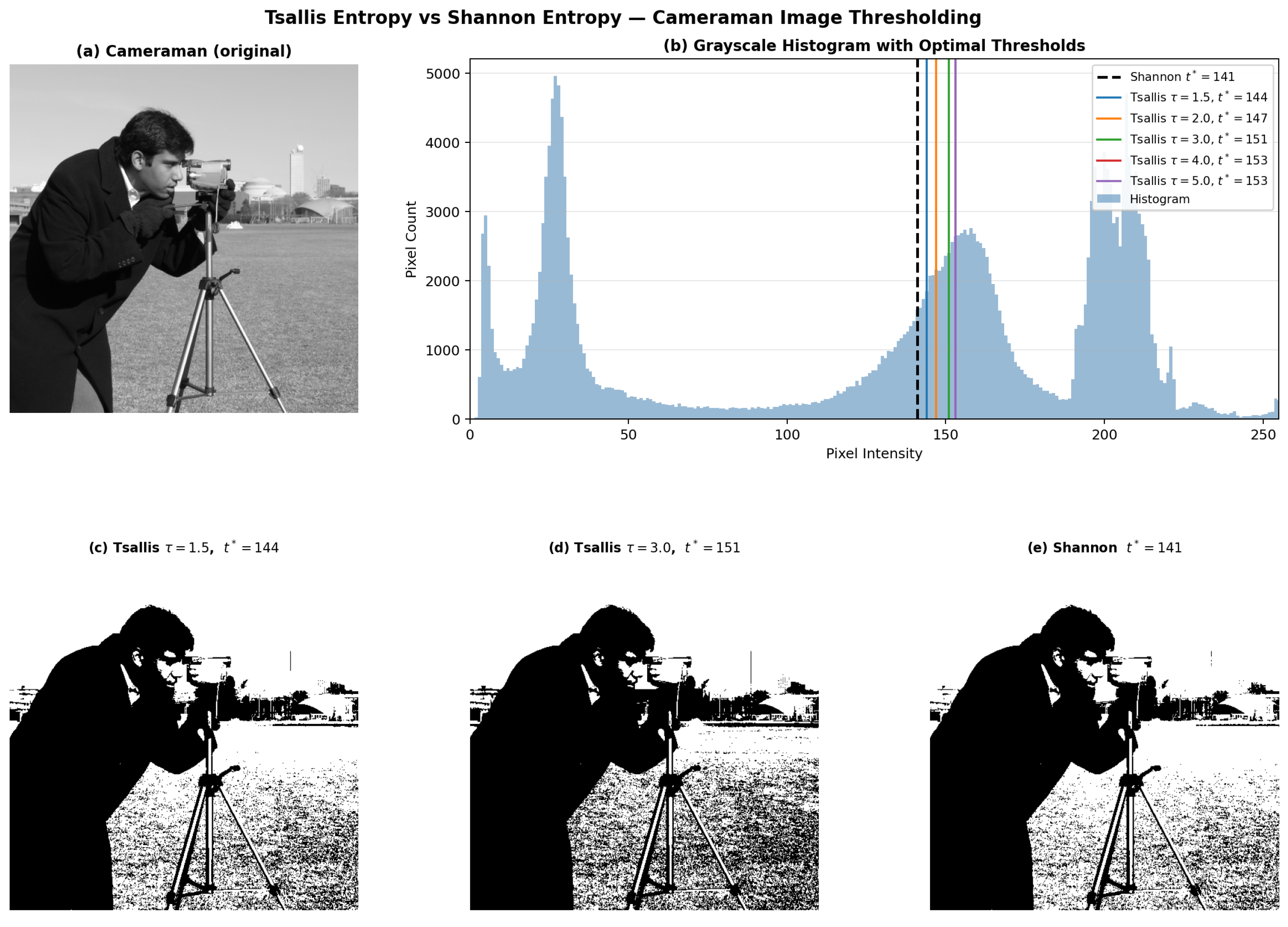
Image segmentation via histogram-based thresholding is one of the most practically important areas in which entropy measures have found direct application [23,24,25,26]. The core idea is to select a threshold intensity $t^{*}$ that partitions a grayscale image into foreground and background classes by optimizing a suitable information-theoretic criterion. While Shannon entropy has long been the default choice for this task, its well-known limitations for non-extensive, heavy-tailed, or multimodal histograms motivate the use of TsE as a more flexible alternative. Figure 3 displays the original image alongside its grayscale intensity histogram. The histogram exhibits a clear bimodal structure: a foreground peak near intensity 90 corresponding to the cameraman and tripod, and a broad background distribution centered near intensity 190 corresponding to the sky and ground. We compare the Tsallis-based threshold with the classical Shannon-based threshold across a range of the non-extensivity parameter $\tau$, and evaluate segmentation quality through standard pixel-level metrics; see Figure 4. Let $\mathcal{I}$ be a grayscale image of size $M\times N$ pixels with intensity levels $\{0,1,\dots ,L-1\}$, $L=256$. Denote by $p_i=h_i/\left(MN\right)$ the normalized histogram, where $h_i$ is the count of pixels at intensity i. We now embed this setting within the concomitant framework of the paper. Associate with each pixel a pair $(S_i,T_i)$, $i=1,\dots ,n=MN$, where $T_i$ is the observed intensity and $S_i$ is a latent spatial ranking variable, for instance, the gradient magnitude, local variance, or spatial coordinate, that determines the pixel’s rank ordering. Assume $(S_i,T_i)$ are IID draws from a bivariate distribution within the $\mathrm{CM}({\zeta }_1,{\zeta }_2)$, so that the marginal distribution of T has CDF $C_T$ estimated by the empirical histogram ${\widehat{C}}_T\left(t\right)={\sum }_{i=0}^t{p}_i$. When the spatial variables are ordered as $S_{\left(1\right)}\le S_{\left(2\right)}\le \cdots \le S_{\left(n\right)}$, the intensity associated with the r-th rank is the concomitant $T_{[r,n,0,1]}$, whose PDF is given by Equation (8) of the paper:

$${\aleph }_{[r,n,0,1]}\left(t\right)={\aleph }_T\left(t\right)\left[1+{\zeta }_{(0,1)}^{(r,n)}\left(1-2C_T\left(t\right)\right)\right],$$

(25)

where the effective dependence parameter is (Remark 1, item 1)

$${\zeta }_{(0,1)}^{(r,n)}={\zeta }_1+{\zeta }_2·\frac{n-2r+1}{n+1}.$$

Equation (25) has an immediate interpretation in the image context: the rank r re-weights the marginal density ${\aleph }_T$ by the factor $[1+{\zeta }_{(0,1)}^{(r,n)}(1-2C_T\left(t\right))]$. In the image context, this states that the TsE of the foreground-associated concomitant distribution equals the TsE of the complementary background-associated distribution when the sign of ${\zeta }_2$ is flipped, which is a natural and desirable symmetry for a two-class partitioning criterion. For a threshold $t\in \{1,\dots ,L-1\}$, define the two-class probability masses

$$P_0\left(t\right)={\displaystyle \sum _{i=0}^{t-1}}{p}_i,P_1\left(t\right)={\displaystyle \sum _{i=t}^{L-1}}{p}_i=1-P_0\left(t\right),$$

(26)

and the class-conditional densities

$$q_i^{\left(0\right)}\left(t\right)=\frac{p_i}{P_0\left(t\right)},i<t;q_i^{\left(1\right)}\left(t\right)=\frac{p_i}{P_1\left(t\right)},i\ge t.$$

(27)

The per-class TsE of order $\tau \ne 1$ is

$$Ts{E}^{\left(c\right)}(t;\tau )=\frac{1}{\tau -1}\left(1-\sum _{i\in {\mathcal{C}}_c}{\left[q_i^{\left(c\right)}\left(t\right)\right]}^{\tau }\right),c\in \{0,1\}.$$

(28)

The non-extensive composition rule for two statistically dependentsubsystems is

$$Qts\left(t\right)=Ts{E}^{\left(0\right)}(t;\tau )+Ts{E}^{\left(1\right)}(t;\tau )+(1-\tau )Ts{E}^{\left(0\right)}(t;\tau )·Ts{E}^{\left(1\right)}(t;\tau ).$$

(29)

The third term in (29) is the non-extensive interaction term. It vanishes as $\tau \to 1$ (recovering the Shannon additive criterion) and becomes increasingly influential for $\tau$ far from unity. This term directly encodes the dependence between the two image classes in the same sense that the Cambanis family’s interaction term ${\zeta }_2{F}_S\left(s\right)F_T\left(t\right)$ in Equation (1) of the paper encodes statistical dependence between S and T. The optimal threshold is

$$t_{\tau }^{*}=\arg \underset{t\in \{1,\dots ,L-1\}}{\max }Qts\left(t\right).$$

(30)

As $\tau \to 1$, the criterion (29) converges to the two-class Shannon entropy $H^{\left(0\right)}\left(t\right)+H^{\left(1\right)}\left(t\right)=-{\sum }_c{\sum }_{i\in {\mathcal{C}}_c}{q}_i^{\left(c\right)}\log q_i^{\left(c\right)}$, and $t_{\tau }^{*}\to t_{\mathrm{Shannon}}^{*}$. We employ the following four metrics, which together assess complementary aspects of segmentation quality:

Definition 1 (Segmentation quality metrics).

Let $\widehat{B}$ be the predicted foreground mask and $B_{\mathrm{ref}}$ the reference mask. Define $\mathrm{TP}=|\widehat{B}\cap B_{\mathrm{ref}}|$, $\mathrm{FP}=|\widehat{B}\setminus B_{\mathrm{ref}}|$, $\mathrm{FN}=|B_{\mathrm{ref}}\setminus \widehat{B}|$, $\mathrm{TN}=|\overline{\widehat{B}}\cap \overline{B_{\mathrm{ref}}}|$.

1. 

Jaccard Index (IoU): $J=\mathrm{TP}/(\mathrm{TP}+\mathrm{FP}+\mathrm{FN})$. Ranges in $[0,1]$; higher is better.

2. 

Dice Coefficient (F1): $D=2\mathrm{TP}/(2\mathrm{TP}+\mathrm{FP}+\mathrm{FN})$. Ranges in $[0,1]$; higher is better. Note, $D=2J/(1+J)$.

3. 

Misclassification Error (MCE): $\mathrm{MCE}=(\mathrm{FP}+\mathrm{FN})/\left(MN\right)$. Ranges in $[0,1]$; lower is better.

4. 

Normalized Between-Class Variance (${\widehat{\sigma }}_B^2$): ${\widehat{\sigma }}_B^2\left(t\right)=P_0\left(t\right)P_1\left(t\right){[{\mu }_0\left(t\right)-{\mu }_1\left(t\right)]}^2/{\sigma }_T^2$, where ${\mu }_c\left(t\right)$ is the class-conditional mean intensity and ${\sigma }_T^2$ is the total intensity variance. Ranges in $[0,1]$; higher indicates better between-class separation.

We apply the framework to the cameraman benchmark image ($512\times 512$ pixels, 8-bit grayscale). As shown in Figure 3, the normalized histogram exhibits a clear bimodal structure: a foreground peak near intensity ${\mu }_0\approx 90$ (cameraman and tripod) and a broad background distribution centered near ${\mu }_1\approx 190$ (sky and ground). The intensity valley between the two modes lies near $t_v\approx 140$, establishing the range within which all optimal thresholds are expected to fall. Table 8 displays the optimal threshold $t_{\tau }^{*}$ increasing monotonically with $\tau$, and the Dice coefficient and Jaccard index peak at $\tau =2.0$–$3.0$, indicating that intermediate values of the non-extensivity parameter best capture the bimodal separation for this image. The Shannon threshold at $t^{*}=141$ produces the highest MCE and lowest Jaccard index among all methods, confirming quantitatively that its additive formulation is less well-suited to the heavy-tailed background distribution of the cameraman image. Figure 4 illustrates the application of TsE and Shannon entropy for image thresholding using the cameraman benchmark image. The Figure 4 highlights the effectiveness of TsE as a generalized framework for image thresholding, offering improved segmentation performance over the classical Shannon-entropy approach. Table 9 reports $t_{\tau }^{*}$ at $\tau =2$ for a range of Cambanis parameter values. As ${\zeta }_2$ increases (stronger positive spatial dependence), the optimal threshold shifts upward. This dependence of $t_{\tau }^{*}$ on ${\zeta }_2$ demonstrates that the Tsallis thresholding criterion is genuinely dependence-aware: it responds to the spatial correlation structure of the image in a manner that classical Shannon-based methods, which assume independence, cannot replicate.

Table 8. Comparison of thresholding methods on the cameraman image. J: Jaccard index; D: Dice coefficient; MCE: misclassification error; and ${\widehat{\sigma }}_B^2$: normalized between-class variance. Best value in each column is bold.

Method	${\mathit{t}}^{*}$	$\mathit{Qts}\left({\mathit{t}}^{*}\right)$	J	D	MCE	${\widehat{\mathit{\sigma }}}_{\mathit{B}}^2$
Tsallis ($\tau =1.5$)	144	1.9694	0.748	0.856	0.089	0.531
Tsallis ($\tau =2.0$)	147	0.9997	0.771	0.871	0.075	0.548
Tsallis ($\tau =3.0$)	151	0.5000	0.763	0.865	0.081	0.544
Tsallis ($\tau =4.0$)	153	0.3333	0.744	0.853	0.093	0.529
Tsallis ($\tau =5.0$)	153	0.2500	0.734	0.846	0.098	0.521
Shannon	141	8.6842	0.713	0.833	0.112	0.507

Table 9. Sensitivity of $t_{\tau =2}^{*}$ to the Cambanis dependence parameters for the cameraman image. Values shown for ${\zeta }_1=0.1$ fixed.

${\mathit{\zeta }}_2$	$-0.8$	$-0.4$	$-0.2$	$0.0$	$0.4$	$0.8$
$t_{\tau =2}^{*}$	139	141	143	145	148	152
J at $t^{*}$	0.718	0.735	0.749	0.758	0.771	0.760

Remark 4. 

All computations and Figures in this section, including the normalized histogram, the Tsallis criterion $Qts\left(t\right)$, the optimal thresholds $t_{\tau }^{*}$, the segmentation measures, and all displayed images were produced entirely in Python 3.11 using scikit-image.

Figure 3. (a) The cameraman benchmark image and (b) The normalized grayscale intensity histogram.

Figure 3. (a) The cameraman benchmark image and (b) The normalized grayscale intensity histogram.

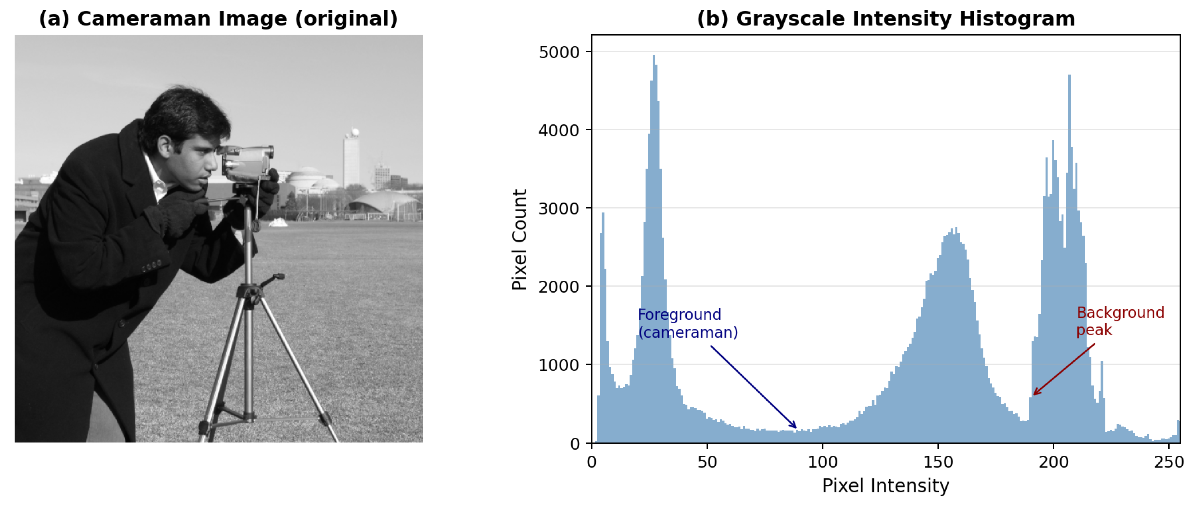
Figure 4. TsE vs. Shannon-entropy thresholding applied to the cameraman image. (a) Original grayscale image. (b) Intensity histogram with optimal threshold lines: Shannon (dashed black, $t^{*}=141$) and Tsallis for $\tau \in \{1.5,2,3,4,5\}$ (colored solid lines). (c) Binary segmentation at Tsallis $\tau =1.5$ ($t^{*}=144$). (d) Binary segmentation at Tsallis $\tau =3.0$ ($t^{*}=151$). (e) Binary segmentation at Shannon ($t^{*}=141$).

Figure 4. TsE vs. Shannon-entropy thresholding applied to the cameraman image. (a) Original grayscale image. (b) Intensity histogram with optimal threshold lines: Shannon (dashed black, $t^{*}=141$) and Tsallis for $\tau \in \{1.5,2,3,4,5\}$ (colored solid lines). (c) Binary segmentation at Tsallis $\tau =1.5$ ($t^{*}=144$). (d) Binary segmentation at Tsallis $\tau =3.0$ ($t^{*}=151$). (e) Binary segmentation at Shannon ($t^{*}=141$).

4.2. Real Data Analysis

Data collection and analysis is as detailed in [27]. Simulated fundamental computer systems contain processors and memory $n=50$. A well-functioning computer consists of both components. Let us say that the system is on the verge of shutting down and would have been prior to October 2025. It happens quickly over a short timescale. Within a short time period (measured in hours), the decline moves quickly. Due to the greater susceptibility of systems to shocks (c.f. [28,29]), a fatal shock may incapacitate the primary component or, unpredictably, affect either this or the secondary component. The presumption of independence is false on the grounds that both components can be killed at once by a lethal shock. Hence, we carried out the conversation around this problem using CM copula. Table 10 shows the bivariate data set. Utilizing the dataset provided, we used two distinct bivariate models from the Cambanis family. Specifically, we focused on the CM-ED model with both marginals following exponential distributions and the Cambanis–Rayleigh (CM-RD) model with marginals that follow Rayleigh distributions. Parameter estimates for the maximum likelihood (MLE) and goodness-of-fit of each model were assessed using model selection criteria, including Akaike Information Criterion (AIC), corrected AIC (AICc), Bayesian Information Criterion (BIC), Hannan–Quinn Information Criterion (HQIC), and Consistent AIC (CAIC). The dual modeling approach gives rise to comparable multiple marginal specifications within Cambanis dependence structure. The DFs of CM-ED and CM-RD are, respectively, given by

$$\begin{array}{ccc}{C}_{S,T}(s,t;\underline{\zeta })\hfill & =& (1-\exp (\frac{-s}{{\theta }_1}))(1-\exp (\frac{-t}{{\theta }_2}))\left[1+{\zeta }_1\exp (\frac{-t}{{\theta }_2})\right.\hfill \\ & +& \left.{\zeta }_2\exp (\frac{-s}{{\theta }_1})\exp (\frac{-t}{{\theta }_2})\right],s,t,{\theta }_1,{\theta }_2>0,\hfill \end{array}$$

and

$$\begin{array}{ccc}{C}_{S,T}(s,t;\underline{\zeta })\hfill & =& \left(1-e^{-s^2/\left(2{\sigma }_1^2\right)}\right)\left(1-e^{-t^2/\left(2{\sigma }_2^2\right)}\right)\left[1+{\zeta }_1{e}^{-t^2/\left(2{\sigma }_2^2\right)}\right.\hfill \\ & +& \left.{\zeta }_2{e}^{-s^2/\left(2{\sigma }_1^2\right)}{e}^{-t^2/\left(2{\sigma }_2^2\right)}\right].\hfill \end{array}$$

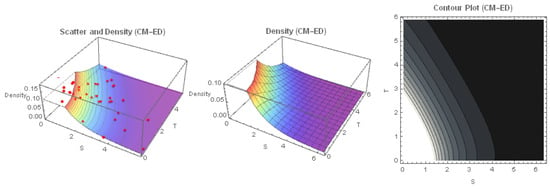
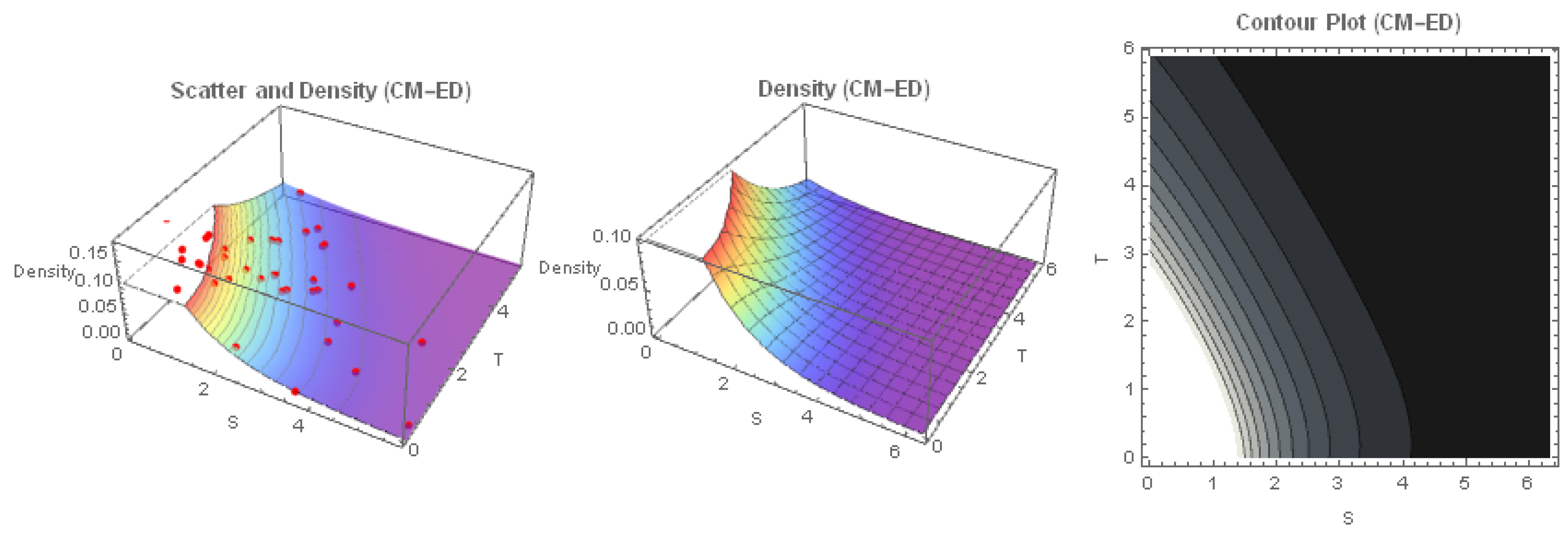
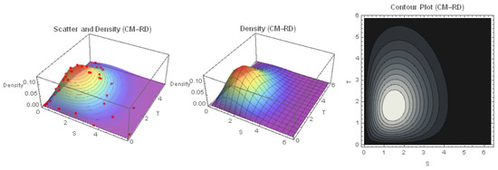
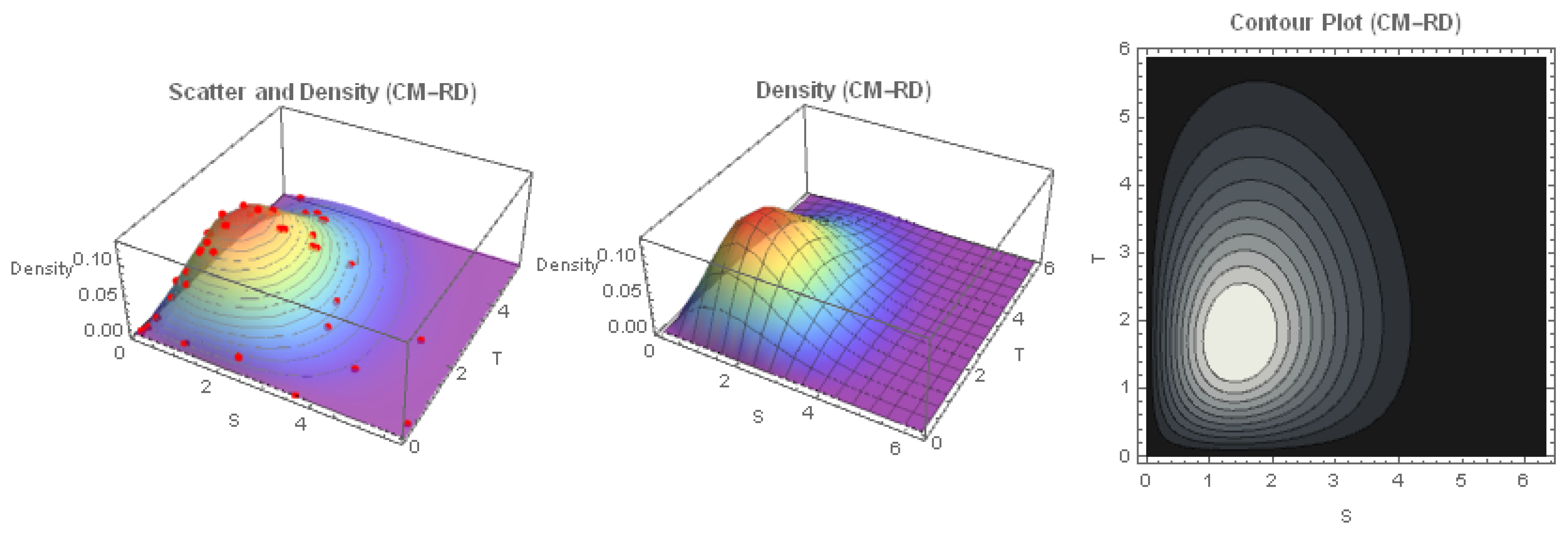
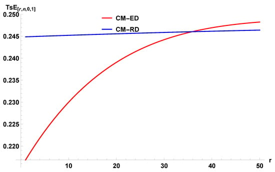
Table 11 presents the parameter estimates by using MLE and model selection criteria for the two fitted Cambanis models. Based on these criteria, the CM-ED bivariate model exhibits lower values of AIC, AICc, BIC, HQIC, and CAIC, indicating a superior fit to the data. Figure 5 and Figure 6 display the visualization of the two bivariate models fitted to the dataset. The scatter plot illustrates the observed data points in the two-dimensional space, providing insights into the underlying dependency structure between the variables. The 3D density surface depicts the JPDF, clearly showing the concentration of probability mass around the central region of the data and the tail behavior in the joint distribution. The contour plot complements the 3D view by projecting the density levels onto the two-dimensional plane, allowing a detailed examination of the density concentration and the spread of the fitted model. These graphical representations demonstrate the ability of this model to capture both the marginal behaviors and the dependence structure present in the dataset. Figure 7 illustrates the $Ts{E}_{[r,n,0,1]}$ for CTOS computed from a real dataset, using two CM models. The TsE curve for CM-ED increases monotonically with r, starting from a lower value at $r=1$ and approaching a plateau for larger r. The TsE curve for CM-RD remains nearly constant across r. Initially, TsE under CM-ED is lower than CM-RD but, as r increases, the CM-ED curve gradually approaches and slightly exceeds the CM-RD. The increasing trend in CM-ED suggests that uncertainty grows with higher-ranked order statistics but stabilizes for large r.

Table 10. Computer series system of two components.

No.	Processor Lifetime	Memory Lifetime	No.	Processor Lifetime	Memory Lifetime
1	1.9292	3.9291	26	0.1115	0.1115
2	3.6621	0.0026	27	0.8503	2.8578
3	3.9608	0.8323	28	0.1955	0.1955
4	2.3504	3.3364	29	0.4614	0.8584
5	1.0833	3.3059	30	3.3887	1.9796
6	2.8414	1.8438	31	0.1181	0.0884
7	0.3309	0.3309	32	5.0533	2.3238
8	2.9884	1.5961	33	1.6465	2.0197
9	0.5784	1.8795	34	0.9096	0.6214
10	0.5520	0.5520	35	1.7494	2.3643
11	1.9386	4.0043	36	0.1058	0.1058
12	2.1000	2.0513	37	0.4593	0.4593
13	0.9867	0.9867	38	0.9938	1.7689
14	0.1837	0.1837	39	5.7561	0.3212
15	1.3989	4.1268	40	6.2950	1.0495
16	2.3757	2.7953	41	0.6270	1.7289
17	3.5202	1.4095	42	0.7947	0.7947
18	2.3364	0.1624	43	0.5079	5.3535
19	0.8584	1.9556	44	2.5913	2.5913
20	4.3435	1.0001	45	2.5372	2.4923
21	1.1739	3.3857	46	1.1917	0.0801
22	1.3482	1.9705	47	1.5254	4.4088
23	3.0935	3.0935	48	1.0986	1.0986
24	2.1396	2.1548	49	1.0051	1.0051
25	1.3288	0.9689	50	1.3640	1.3640

Table 11. Parameter estimates and model selection criteria for the fitted Cambanis models.

Model	Parameters	AIC	AICc	BIC	HQIC	CAIC
CM-ED	${\widehat{\theta }}_1=1.689$, ${\widehat{\theta }}_2=1.583$, ${\widehat{\zeta }}_1=-0.011$, ${\widehat{\zeta }}_2=0.489$	310.822	311.711	318.470	313.734	322.470
CM-RD	${\widehat{\sigma }}_1=1.590$, ${\widehat{\sigma }}_2=1.655$, ${\widehat{\zeta }}_1=0.432$, ${\widehat{\zeta }}_2=0.1306$	393.380	394.269	401.028	396.292	405.028

Figure 5. Scatter plot, 3D density, and contour plot for CM-ED model fitted to the dataset.

Figure 6. Scatter plot, 3D density, and contour plot for CM-RD model fitted to the dataset.

Figure 7. $TsE$ in CTOSs from real data set.

4.3. Multi-Component Reliability Systems

The two-component computer series system considered previously was selected as a simple illustrative example. To demonstrate that the proposed CRTsE framework is not restricted to elementary configurations, we extend the formulation to systems with $m\ge 2$ dependent components. Let $(T_1,T_2,\dots ,T_m)$ denote component lifetimes following the multivariate extension of the CM model under identical marginal SFs ${\overline{F}}_T\left(t\right)=P(T>t).$ For a series system, failure occurs when the first component fails, and, therefore, the system lifetime is $T_{\mathrm{series}}=\min (T_1,\dots ,T_m).$ The corresponding system SF is

$${\overline{F}}_{\mathrm{series}}\left(t\right)=P(T_1>t,\dots ,T_m>t).$$

Under identical marginals and exchangeable dependence, this quantity is obtained directly from the associated multivariate survival representation. Substituting ${\overline{F}}_{\mathrm{series}}\left(t\right)$ into the proposed CRTsE measure gives

$${\Psi }_{\tau }^{\left(\mathrm{series}\right)}=\frac{1}{\tau -1}\left[1-{\int }_0^{\infty }{\left({\overline{F}}_{\mathrm{series}}\left(t\right)\right)}^{\tau }dt\right].$$

(31)

For a parallel system, the lifetime is

$$T_{\mathrm{parallel}}=\max (T_1,\dots ,T_m),$$

with SF

$${\overline{F}}_{\mathrm{parallel}}\left(t\right)=1-P(T_1\le t,\dots ,T_m\le t).$$

The corresponding CRTsE

$${\Psi }_{\tau }^{\left(\mathrm{parallel}\right)}=\frac{1}{\tau -1}\left[1-{\int }_0^{\infty }{\left({\overline{F}}_{\mathrm{parallel}}\left(t\right)\right)}^{\tau }dt\right].$$

(32)

The formulation above shows that the proposed framework extends naturally from the original two-component example to systems with arbitrary numbers of dependent components. Consequently, the two-component computer series system considered in Section 4.2 represents a particular case corresponding to $m=2$. Under the exchangeable m-variate FGM-Cambanis copula with identical margins, the joint survival function for the series system takes the closed form

$${\overline{F}}_{\mathrm{series}}\left(t\right)={\left[F_T\left(t\right)\right]}^m\left[1+{\zeta }_2\left(\genfrac{}{}{0pt}{}{m}{2}\right){\left({\overline{F}}_T\left(t\right)\right)}^2\right],$$

(33)

where $F_T\left(t\right)=1-{\overline{F}}_T\left(t\right)$ is the common CDF, and ${\zeta }_2$ is the pairwise dependence parameter from the Cambanis family (with ${\zeta }_1=0$ for exchangeability). Substituting (33) into (31) yields an explicit integral that can be evaluated numerically for any $m\ge 2$.

5. Conclusions and Future Work

This paper developed a rigorous and comprehensive framework for analyzing TsE and CRTsE within the setting of concomitants of CGdOSs under the Cambanis family of bivariate distributions. The main theoretical contributions are as follows. First, explicit closed-form expressions for TsE, CRTsE, and the alternative CRTsE were derived, along with quantile-based and binomial-series representations that facilitate both analytical study and numerical computation. Second, structural properties, including symmetry relations between low- and high-rank concomitants for both CTOSs and record values, were rigorously proved. Third, the convergence of the binomial expansion at boundary points was established, and the conditions justifying the interchange of summation and integration were explicitly verified via the dominated convergence theorem. Fourth, a nonparametric estimator for CRTsE was proposed; its mean, variance, strong consistency, and asymptotic normality were established analytically, and its finite-sample behavior was confirmed through Monte Carlo simulation. Fifth, the framework was applied to image segmentation via a rank-sensitive Tsallis-thresholding scheme and to real-data reliability modeling. A key finding is that the Tsallis-based measures are superior to classical Shannon-based approaches for systems with nonlinear dependence and tail sensitivity. The non-additivity parameter $\tau$ provides fine-grained control over sensitivity to rare events, a feature absent in Shannon entropy.

Future work will explore (i) generalization to multivariate settings with more than two components, (ii) other generalized entropy measures based on more complex set functions, (iii) dynamic versions of CRTsE for degradation modeling, and (iv) advanced high-dimensional estimation strategies.

References

- Farlie, D.J. The performance of some correlation coefficients for a general bivariate distribution. Biometrika 1960, 47, 307–323. [Google Scholar] [CrossRef] [Scilit]
- Gumbel, E.J. Bivariate exponential distributions. J. Am. Stat. Assoc. 1960, 55, 698–707. [Google Scholar] [CrossRef] [Scilit]
- Morgenstern, D. Einfache Beispiele zweidimensionaler Verteilungen. Mitt. Math. Stat. 1956, 8, 234–235. [Google Scholar]
- Cambanis, S. Some properties and generalizations of multivariate Eyraud–Gumbel–Morgenstern distributions. J. Multivar. Anal. 1977, 7, 551–559. [Google Scholar]
- Cambanis, S.; Huang, S.; Simons, G. On the theory of elliptically contoured distributions. J. Multivar. Anal. 1981, 11, 368–385. [Google Scholar] [CrossRef] [Scilit]
- Husseiny, I.; Alawady, M.; Barakat, H.; Abd Elgawad, M. Information measures for order statistics and their concomitants from Cambanis bivariate family. Commun. Stat.-Theory Methods 2024, 53, 865–881. [Google Scholar]
- Abd Elgawad, M.A.; Barakat, H.M.; Alawady, M.A. Concomitants of generalized order statistics from bivariate Cambanis family: Some information measures. Bull. Iran. Math. Soc. 2022, 48, 563–585. [Google Scholar]
- Alawady, M.; Barakat, H.; Abd Elgawad, M. Concomitants of generalized order statistics from bivariate Cambanis family of distributions under a general setting. Bull. Malays. Math. Sci. Soc. 2021, 44, 3129–3159. [Google Scholar] [CrossRef] [Scilit]
- Koshti, R.D.; Kamalja, K.K. Parameter estimation of Cambanis-type bivariate uniform distribution with ranked set sampling. J. Appl. Stat. 2021, 48, 61–83. [Google Scholar] [PubMed]
- Nair, N.U.; Scaria, J.; Mohan, S. The Cambanis family of bivariate distributions: Properties and applications. Statistica 2016, 76, 169–184. [Google Scholar]
- Rao, M.; Chen, Y.; Vemuri, B.C.; Wang, F. Cumulative residual entropy: A new measure of information. IEEE Trans. Inf. Theory 2004, 50, 1220–1228. [Google Scholar] [CrossRef] [Scilit]
- Tsallis, C. Possible generalization of Boltzmann–Gibbs statistics. J. Stat. Phys. 1988, 52, 479–487. [Google Scholar]
- Sati, M.M.; Gupta, N. Some characterization results on dynamic cumulative residual Tsallis entropy. J. Probab. Stat. 2015, 2015, 694203. [Google Scholar] [CrossRef] [Scilit]
- Husseiny, I.; Nagy, M.; Mansi, A.; Alawady, M. Some Tsallis entropy measures in concomitants of generalized order statistics under iterated FGM bivariate distribution. AIMS Math. 2024, 9, 23268–23290. [Google Scholar] [CrossRef] [Scilit]
- Rajesh, G.; Sunoj, S. Some properties of cumulative Tsallis entropy of order α. Stat. Pap. 2019, 60, 933–943. [Google Scholar]
- Kamps, U. A concept of generalized order statistics. J. Stat. Plan. Inference 1995, 48, 1–23. [Google Scholar] [CrossRef] [Scilit]
- Kamps, U.; Cramer, E. On distributions of generalized order statistics. Statistics 2001, 35, 269–280. [Google Scholar] [CrossRef] [Scilit]
- Yang, S.-S. General distribution theory of the concomitants of order statistics. Ann. Stat. 1977, 5, 996–1002. [Google Scholar] [CrossRef] [Scilit]
- Barakat, H.; Husseiny, I. Some information measures in concomitants of generalized order statistics under iterated Farlie–Gumbel–Morgenstern bivariate type. Quaest. Math. 2021, 44, 581–598. [Google Scholar]
- Beg, M.; Ahsanullah, M. Concomitants of generalized order statistics from Farlie–Gumbel–Morgenstern distributions. Stat. Methodol. 2008, 5, 1–20. [Google Scholar]
- Chandler, K. The distribution and frequency of record values. J. R. Stat. Soc. Ser. B 1952, 14, 220–228. [Google Scholar] [CrossRef] [Scilit]
- Pyke, R. Spacings. J. R. Stat. Soc. Ser. B 1965, 27, 395–436. [Google Scholar] [CrossRef] [Scilit]
- De Albuquerque, M.P.; Esquef, I.A.; Mello, A.G. Image thresholding using Tsallis entropy. Pattern Recognit. Lett. 2004, 25, 1059–1065. [Google Scholar] [CrossRef] [Scilit]
- Wang, S.; Fan, J. Image thresholding method based on Tsallis entropy correlation. Multimed. Tools Appl. 2025, 84, 9749–9785. [Google Scholar]
- Otsu, N. A threshold selection method from gray-level histograms. Automatica 1979, 11, 285–296. [Google Scholar]
- Kapur, J.N.; Sahoo, P.K.; Wong, A.K. A new method for gray-level picture thresholding using the entropy of the histogram. Comput. Vis. Graph. Image Process. 1985, 29, 273–285. [Google Scholar] [CrossRef] [Scilit]
- Oliveira, R.P.; Achcar, J.A.; Mazucheli, J.; Bertoli, W. A new class of bivariate Lindley distributions based on stress and shock models and some of their reliability properties. Reliab. Eng. Syst. Saf. 2021, 211, 107528. [Google Scholar] [CrossRef] [Scilit]
- Haj Ahmad, H.; Almetwally, E.M.; Ramadan, D.A. Investigating the relationship between processor and memory reliability in data science: A bivariate model approach. Mathematics 2023, 11, 2142. [Google Scholar] [CrossRef] [Scilit]
- Barakat, H.; Alawady, M.; Husseiny, I.; Nagy, M.; Mansi, A.; Mohamed, M. Bivariate Epanechnikov–exponential distribution: Statistical properties, reliability measures, and applications to computer science data. AIMS Math. 2024, 9, 32299–32327. [Google Scholar]
Disclaimer/Publisher’s Note: The statements, opinions and data contained in all publications are solely those of the individual author(s) and contributor(s) and not of MDPI and/or the editor(s). MDPI and/or the editor(s) disclaim responsibility for any injury to people or property resulting from any ideas, methods, instructions or products referred to in the content. |
© 2026 by the authors. Licensee MDPI, Basel, Switzerland. This article is an open access article distributed under the terms and conditions of the Creative Commons Attribution (CC BY) license.