Stochastic Differential Financial Portfolio Game Under CEV Model with CRRA Utility

Abstract

This paper investigates a stochastic differential portfolio game between two competing investors with relative wealth preferences. The financial market consists of one risk-free asset and one risky asset, whose price dynamics follow the CEV model. We formulate this game as two utility maximization problems, where each investor aims to maximize their relative utility defined as the weighted average of the ratio between their terminal wealth and the competitor’s terminal wealth. Firstly, we derive the Hamilton–Jacobi–Bellman (HJB) equations and corresponding value functions through the dynamic programming principle. Next, we obtain the explicit solutions to equilibrium investment strategies and value functions for the non-zero-sum game under the CRRA utility framework. Finally, we conducted numerical simulations to analyze the impacts of model parameters on equilibrium strategies and provide relevant economic explanations.

1. Introduction

Portfolio theory, which focuses on efficient asset allocation by maximizing returns and minimizing risks, has long been a core research topic in modern finance. Theoretical models vary across different types of investors, including retail investors and institutional investors such as funds and insurance companies. Retail investors make decisions independently based on their risk appetite and market conditions, while institutional investors interact closely with one another.

With the development of financial markets, institutional investors have gained growing market influence. To outperform their peers, they must incorporate competitors’ behaviors into their investment decisions. In fund management, the ranking effect in behavioral finance drives investors to favor top-tier fund companies. Accordingly, fund managers are motivated to beat their peers to attract capital inflows and boost performance. In addition, from the perspective of investment behavior psychology, investors also pursue higher social status and thus care greatly about their relative performance. Such competitive interactions have attracted extensive academic attention. As Hortaçsu and Syverson (2004) [1] pointed noted, the mutual fund literature has generally not addressed strategic interaction among firms. Yet, competitive forces are important determinants of the fortunes of asset management firms.

In financial markets, the competition between institutional investors is usually measured by relative performance indicators. In practice, relative performance can better reflect the professional capability of investment manager, and it has been widely adopted as a benchmark for performance evaluation in the financial industry (Dong et al., 2023 [2]). In academic research, two mainstream methods are used to characterize relative performance: the first calculates the weighted average of the performance gap between an investor and their competitors, and the second adopts the weighted average of the performance ratio between peers. The former has received far more research attention.

Espinosa and Touzi (2015) [3] first introduced relative performance to characterize strategic competition among N investment managers. They constructed an N-player investment game within the classical Black–Scholes setting and proved the existence of Nash equilibrium, laying a solid theoretical basis for investment decisions with multi-agent strategic interactions. Following their framework, Li and Qiu (2025) [4] examined a non-zero-sum portfolio game of optimal asset-liability management (ALM) between insurers and reinsurers within the framework of the constant elasticity of variance (CEV) model under common shock dependence. For cases of power utility and mean-variance utility, Luo and Zhou (2025) [5] obtained explicit expressions of the investment strategies and value functions for asset-liability management. Yang et al. (2020) [6] further extended this research stream by incorporating liabilities and adopting the Heston stochastic volatility model for risky asset prices.

In actuarial research, Bensoussan et al. (2014) [7] initially adopted relative performance to describe competition between insurance companies. They explored a two-player non-zero-sum game of investment and reinsurance and analyzed corresponding optimal strategies under competitive setting. Subsequently, a large number of scholars later extended their model to further study similar non-zero-sum games for insurers, such as Siu et al. (2017) [8], Deng et al. (2018) [9], Bin and Zhu (2021) [10], Bin et al. (2024) [11], and Bai et al. (2022) [12], along with their cited works. All of the above literature focuses on continuous-time investment or investment–reinsurance games. Zhou et al. (2019) [13,14] explored multi-stage portfolio and investment games with serially correlated asset returns. Lin et al. (2020) [15] further investigated a discrete-time portfolio game between two competing institutional investors whose decisions interact with each other. Their results show that the findings from discrete-time frameworks are consistent with those obtained in continuous-time models.

In contrast, studies on the second type of relative performance measurement remain relatively scarce. As a seminal work, Basak and Makarov (2014) [16] conducted a comprehensive analysis of strategic interactions in dynamic asset allocation and discussed how portfolio choices and professional specialization interact among fund managers. Lacker and Zariphopoulou (2019) [17] adopted N-player differential games and mean-field game theory to solve multi-agent investment decision problems. They derived explicit analytical expressions for equilibrium strategies under both exponential and power utility assumptions. Building upon this foundation, Lacker and Soret (2020) [18] extended the above framework by incorporating consumption decisions and studied an N-player non-zero-sum investment–consumption game. In an incomplete market, Kraft et al. (2020) [19] discussed a two-player non-zero-sum investment game where risky asset prices follow an extended Heston model. Using the dynamic programming principle, they also obtained closed-form solutions for equilibrium investment strategies. Zhu et al. (2026) [20] has also extended the research on relative performance optimal investment–reinsurance problems to the setting of incomplete financial markets.

The literature review indicates that few studies have explored portfolio games with relative performance under the CEV model. Against this background, this study constructs a continuous-time two-player stochastic investment game model. We adopt the Constant Relative Risk Aversion (CRRA) utility function to describe investors’ risk preferences (Wu and Ma, 2015 [21]), and define relative performance as the weighted average of the wealth ratio between each investor and their competitor. Each investor’s objective is to maximize the expected utility of terminal relative wealth. By applying the dynamic programming principle, we further derive the explicit analytical solutions to the Nash equilibrium strategies.

The main contributions of this paper are as follows:

(1)

Specifically, we employ relative performance, defined as the weighted average of an investor’s terminal wealth ratio relative to that of the competitor, to characterize the competitive interaction between two investors. On this basis, we build a two-player non-zero-sum investment game where risky asset prices obey the CEV model.

(2)

Based on the dynamic programming principle, we prove the existence conditions of Nash equilibrium strategies and derive the explicit analytical solutions of Nash equilibrium under the CRRA utility framework. These expressions are valuable because they allow us to intuitively observe the direct impact of each parameter on the equilibrium strategy. This analytical tractability further facilitates optimal parameter design and boundary analysis, offering clear portfolio insights that would be obscured in purely numerical approaches.

2. Model Assumptions and Construction

Let $(\mathsf{\Omega },\mathbb{F},\mathbb{P})$ denote a complete probability space, where $\mathbb{P}$ stands for the probability measure and the filtration $\mathbb{F}\triangleq \{{\mathcal{F}}_t{\}}_{t\ge 0}$ satisfies the usual conditions (i.e., it is right-continuous and complete). Here, ${\left\{{\mathcal{F}}_t\right\}}_{t\ge 0}$ represents all available information up to time t. All stochastic processes and random variables in this paper are defined on this probability space. We further assume continuous trading, permissible short-selling, and the absence of transaction costs and taxes in the financial.

2.1. Model Assumptions

For simplicity and without loss of generality, we consider a financial market with two types of financial assets: one risk-free bond and one risky asset, such as a stock. Assume that the price of the risk-free bond $B(t)$ follows the ordinary differential of Equation (1):

$$dB(t)=rB(t)dt$$

(1)

where $r>0$ stand for the risk-free interest rate. The price of the risky asset $S(t)$ follows the CEV model shown in Equation (2).

$$dS(t)=\mu S(t)dt+\sigma S^{\beta +1}(t)dw(t)$$

(2)

In this model, the constant $\mu >0$ represents the expected return rate of the risky asset, where $\sigma >0$ is a given constant; $\beta$ is known as the constant elasticity of variance factor; $\sigma S^{\beta }(t)$ denotes the instantaneous volatility of the risky asset; and $w(t)$ is a one-dimensional standard Brownian motion.

Assume that at any time $t$, an investor allocates a proportion $\pi (t)$ of wealth to the risky asset, and the rest $1-\pi (t)$ to the risk-free bond. We use $\pi (t)$ to denote the investor’s investment strategy. Then, under this strategy $\pi (t)$, the investor’s wealth dynamics satisfy the stochastic differential below (Equation (3)).

$$\begin{gathered} dX(t)=\left[1-\pi (t)\right]X(t){\displaystyle \frac{dB(t)}{B(t)}}+\pi (t)X(t){\displaystyle \frac{dS(t)}{S(t)}} \\ \hspace{1em}\hspace{1em}\hspace{1em}\hspace{1em}\hspace{1em}\hspace{1em}=\left[r+(\mu -r)\pi (t)\right]X(t)dt+\pi (t)X(t)\sigma S^{\beta }(t)dw(t). \end{gathered}$$

(3)

In financial markets, numerous investors often interact strategically rather than making decisions independently, which essentially forms a stochastic economic game. This paper focuses on two competing investors, namely two insurance companies or two fund management firms, labeled as investor 1 and investor 2, respectively. The investment strategy of investor $k \in \{1, 2\}$ is denoted as ${\pi }_k(t)$. Accordingly, the wealth process $X_k(t)$ of investor $k$ under strategy ${\pi }_k(t)$ can be expressed as

$$d{X}_k(t)=\left[r+(\mu -r){\pi }_k(t)\right]X_k(t)dt+{\pi }_k(t)X_k\sigma S^{\beta }(t)dw(t)$$

(4)

Definition 1 (Admissible Strategy).

For $k \in \{1, 2\}$, a strategy ${\pi }_k(t)$ is called admissible for investor $k$ if the following two conditions hold:

 (i) 

${\pi }_k(t)$ is ${\mathcal{F}}_t-$ progressively measurable and holds for any $\mathbb{E}\left[{\int }_0^T\left|\right|{\pi }_k(t)|{|}^{2}dt\right]<\infty$;

 (ii) 

For a given $\forall x_0 \in \mathbb{R}$, the stochastic differential Equation (4) has a unique strong solution $X_k(t)$, satisfying  $\mathbb{E}\left[\underset{0\le t\le T}{\sup }\left|\right|X_k(t)|{|}^2\right]<\infty$ almost surely for all $T<\infty$.

Denote the set of all admissible strategies for investor $k$ as $k=1, 2$.

2.2. Construction of the Non-Zero-Sum Game Model

We study a two-player non-zero-sum investment game under a complete information framework. Let  $U_k(\cdot )$ denote the utility function of investor $k$, which is smooth, strictly increasing, and strictly concave ($U_k^{\prime }(\cdot )>0$ and $U_k^{″}(\cdot )<0$). Each investor aims to choose an admissible strategy ${\pi }_k\in {\mathsf{\Pi }}_k$ to maximize the expected utility of their terminal wealth. In this model, investors pay attention to both the absolute wealth and relative wealth of competitors. Specifically, the optimization problem for each investor can be formulated as follows:

Given the strategy choice ${\pi }_j\in {\mathsf{\Pi }}_j$ of the competitor $j \in \{1, 2\}$, investor $k\ne j$ seeks an optimal strategy to maximize the objective function (5).

$$\underset{{\pi }_k\in {\mathsf{\Pi }}_k}{\text{sup}}{J}_k(t,x_k,x_j,{\pi }_k,{\pi }_j)=J_k(t,x_k,x_j,{\pi }_k^{*},{\pi }_j)$$

(5)

where

$$\begin{gathered} J_k(t,x_k,x_j,{\pi }_k,{\pi }_j)\triangleq \mathbb{E}\left[U_k\left(X_k^{1-{\kappa }_k}(T){\left({\displaystyle \frac{X_k(T)}{X_j(T)}}\right)}^{{\kappa }_k}\right)\left|X_k(t)=x_k,X_j(t)=x_j\right.\right] \\ \hspace{1em}\hspace{1em}\hspace{1em} =\mathbb{E}\left[U_k\left(X_k(T)X_j^{-{\kappa }_k}(T)\right)\left|X_k(t)=x_k,X_j(t)=x_j\right.\right] \end{gathered}$$

The first term in the above expression $X_k^{1-{\kappa }_k}(T)$ measures the investor’s utility derived from absolute wealth, and the second term ${\left({\displaystyle \frac{X_k(T)}{X_j(T)}}\right)}^{{\kappa }_k}$ measures the utility derived from relative wealth. The parameter ${\kappa }_k\in [0, 1]$ reflects how sensitive the investor $k$ is to the competitor’s ($j\ne k$) wealth, and it also quantifies the degree of market competition. A larger value of this parameter means investor $k$ attaches more importance to relative wealth utility. In extreme cases, when ${\kappa }_k=0$, investor $k$ only focuses on absolute wealth utility; conversely, when ${\kappa }_k=1$, investor $k$ cares exclusively about relative wealth utility.

Referring to Espinosa and Touzi (2015) [3], the optimization problem (5) can be transformed into the following non-zero-sum game problem.

We aim to find the Nash equilibrium strategy pair $({\pi }_1^{*},{\pi }_2^{*})\in {\mathsf{\Pi }}_1\times {\mathsf{\Pi }}_2$ such that for any admissible strategies ${\pi }_1\in {\mathsf{\Pi }}_1$ and ${\pi }_2\in {\mathsf{\Pi }}_2$, the following inequalities hold:

$$\left\{\begin{array}{c}{J}_1\left(t,x_1,x_2,{\pi }_1,{\pi }_2^{*}\right)\le J_1\left(t,x_1,x_2,{\pi }_1^{*},{\pi }_2^{*}\right),\\ J_2\left(t,x_2,x_1,{\pi }_2,{\pi }_1^{*}\right)\le J_2\left(t,x_2,x_1,{\pi }_2^{*},{\pi }_1^{*}\right).\end{array}\right.$$

3. Solution of the Non-Zero-Sum Game Model

This section adopts the dynamic programming principle to derive the Nash equilibrium strategies for the proposed non-zero-sum game. $\forall t\in [0,T]$ and $j\ne k\in \{1, 2\}$, and given $X_k(t)=x_k$, $X_j(t)=x_j$, and $S(t)=s$, the value function $V_k(t,x_k,x_j,s)$ of investor $k$ is defined as Equation (6):

$$V_k(t,x_k,x_j,s)=\underset{{\pi }_k\in {\mathsf{\Pi }}_k}{\text{sup}}\mathbb{E}\left[U_k\left(X_k(T)X_j^{-{\kappa }_k}(T)\right)|X_k(t)=x_k,X_j(t)=x_j,S(t)=s\right]$$

(6)

According to the stochastic dynamic programming principle (Richard, 1957 [22]; Liberzon, 2012 [23]), the value function $V_k(t,x_k,x_j,s)$ satisfies the Hamilton–Jacobi–Bellman (HJB) (Equation (7))

$$\begin{array}{l}\underset{{\pi }_k\in {\mathsf{\Pi }}_k}{\text{sup}}\left\{{\displaystyle \frac{\partial V_k}{\partial t}}+\left[r{x}_k+(\mu -r){\pi }_k{x}_k\right]{\displaystyle \frac{\partial V_k}{\partial x_k}}+{\displaystyle \frac{1}{2}}{\sigma }^2{s}^{2\beta }{\pi }_k^2{x}_k^2{\displaystyle \frac{{\partial }^2{V}_k}{\partial x_k^2}}+{\sigma }^2{s}^{2\beta +1}{\pi }_k{x}_k\right.{\displaystyle \frac{{\partial }^2{V}_k}{\partial x_k\partial s}}\\ \hspace{1em}\hspace{1em}+{\sigma }^2{s}^{2\beta }{\pi }_k{\pi }_j^{*}{x}_k{x}_j{\displaystyle \frac{{\partial }^2{V}_k}{\partial x_k\partial x_j}}+\left[r{x}_j+(\mu -r){\pi }_j^{*}{x}_j\right]{\displaystyle \frac{\partial V_k}{\partial x_j}}+{\displaystyle \frac{1}{2}}{\sigma }^2{s}^{2\beta }{\pi }_j^{*2}{x}_j^2{\displaystyle \frac{{\partial }^2{V}_k}{\partial x_j^2}}\\ \hspace{1em}\hspace{1em}\left.+{\sigma }^2{s}^{2\beta +1}{\pi }_j^{*}{x}_j{\displaystyle \frac{{\partial }^2{V}_k}{\partial x_j\partial s}}+\mu s{\displaystyle \frac{\partial V_k}{\partial s}}+{\displaystyle \frac{1}{2}}{\sigma }^2{s}^{2\beta +2}{\displaystyle \frac{{\partial }^2{V}_k}{\partial s^2}}\right\}=0,\end{array}$$

(7)

along with its corresponding terminal condition $V_k(T,x_k,x_j,s)=U_k\left(x_k{x}_j^{-{\kappa }_k}\right)$.

We take the first-order derivative of Equation (7) with respect to ${\pi }_k$ and obtain Equation (8).

$${\pi }_k^{*}=-\underset{\mathrm{myopic}\hspace{1em}\mathrm{term}}{\underbrace{{\displaystyle \frac{(\mu -r)x_k\frac{\partial V_k}{\partial x_k}}{{\sigma }^2{s}^{2\beta }{x}_k^2\frac{{\partial }^2{V}_k}{\partial x_k^2}}}}}-\underset{\mathrm{hedging}\hspace{1em}\mathrm{term}}{\underbrace{{\displaystyle \frac{{\sigma }^2{s}^{2\beta +1}{x}_k\frac{{\partial }^2{V}_k}{\partial x_k\partial s}}{{\sigma }^2{s}^{2\beta }{x}_k^2\frac{{\partial }^2{V}_k}{\partial x_k^2}}}}}-\underset{\mathrm{adjustment}\hspace{1em}\mathrm{term}}{\underbrace{{\displaystyle \frac{{\sigma }^2{s}^{2\beta }{\pi }_j^{*}{x}_k{x}_j\frac{{\partial }^2{V}_k}{\partial x_k\partial x_j}}{{\sigma }^2{s}^{2\beta }{x}_k^2\frac{{\partial }^2{V}_k}{\partial x_k^2}}}}}.$$

(8)

As shown in this formula, the optimal investment strategy ${\pi }_k^{*}$ of investor $k$ consists of three parts. The first term corresponds to the so-called myopic term, the second is the hedging term that accounts for the price volatility of the risky asset, and the third is an adjustment term induced by competition between investors. Therefore, an extra adjustment term emerges in Equation (8) relative to the case without competition.

Substituting Equation (8) into the HJB Equation (7), we simplify the original HJB equation and derive the partial differential Equation (9) below:

$$\begin{array}{l}{\displaystyle \frac{\partial V_k}{\partial t}}+\mu s{\displaystyle \frac{\partial V_k}{\partial s}}+{\displaystyle \frac{1}{2}}{\sigma }^2{s}^{2\beta +2}{\displaystyle \frac{{\partial }^2{V}_k}{\partial s^2}}+r{x}_k{\displaystyle \frac{\partial V_k}{\partial x_k}}-{\displaystyle \frac{1}{2}}{\sigma }^2{s}^{2\beta }{\pi }_k^{*2}{x}_k^2{\displaystyle \frac{{\partial }^2{V}_k}{\partial x_k^2}}\\ +\left[r{x}_j+(\mu -r){\pi }_j^{*}{x}_j\right]{\displaystyle \frac{\partial V_k}{\partial x_j}}+{\displaystyle \frac{1}{2}}{\sigma }^2{s}^{2\beta }{\pi }_j^{*2}{x}_j^2{\displaystyle \frac{{\partial }^2{V}_k}{\partial x_j^2}}+{\sigma }^2{s}^{2\beta +1}{\pi }_j^{*}{x}_j{\displaystyle \frac{{\partial }^2{V}_k}{\partial x_j\partial s}}=0.\end{array}$$

(9)

Based on the above analysis, we further derive the sufficient conditions for the existence of Nash equilibrium for the proposed game, which are summarized in Theorem 1 below.

Theorem 1.

$\forall (t,x_k,x_j,s)\in [0,T]\times {\mathbb{R}}^3$, if  ${\displaystyle \frac{{\partial }^2{V}_k}{\partial x_k^2}}\ne 0$, then the Nash equilibrium strategies of the game satisfy the coupled nonlinear Equation (10):

$$\left\{\begin{array}{c}{\pi }_1^{*}(t)=-{\displaystyle \frac{(\mu -r)x_1\frac{\partial V_1}{\partial x_1}+{\sigma }^2{s}^{2\beta +1}{x}_1\frac{{\partial }^2{V}_1}{\partial x_1\partial s}+{\sigma }^2{s}^{2\beta }{\pi }_2^{*}{x}_1{x}_2\frac{{\partial }^2{V}_1}{\partial x_1\partial x_2}}{{\sigma }^2{s}^{2\beta }{x}_1^2\frac{{\partial }^2{V}_1}{\partial x_1^2}}},\\ {\pi }_2^{*}(t)=-{\displaystyle \frac{(\mu -r)x_2\frac{\partial V_2}{\partial x_2}+{\sigma }^2{s}^{2\beta +1}{x}_2\frac{{\partial }^2{V}_2}{\partial x_2\partial s}+{\sigma }^2{s}^{2\beta }{\pi }_1^{*}{x}_1{x}_2\frac{{\partial }^2{V}_2}{\partial x_1\partial x_2}}{{\sigma }^2{s}^{2\beta }{x}_2^2\frac{{\partial }^2{V}_2}{\partial x_2^2}}},\end{array}\right.$$

(10)

Here,  $V_1$ and  $V_2$ are solutions to the coupled partial differential Equation (11) subject to the terminal conditions (12).

$$\left\{\begin{array}{l}{\displaystyle \frac{\partial V_1}{\partial t}}+\mu s{\displaystyle \frac{\partial V_1}{\partial s}}+{\displaystyle \frac{1}{2}}{\sigma }^2{s}^{2\beta +2}{\displaystyle \frac{{\partial }^2{V}_1}{\partial s^2}}+r{x}_1{\displaystyle \frac{\partial V_1}{\partial x_1}}-{\displaystyle \frac{1}{2}}{\sigma }^2{s}^{2\beta }{\pi }_1^{*2}{x}_1^2{\displaystyle \frac{{\partial }^2{V}_1}{\partial x_1^2}}\\ +\left[r{x}_2+(\mu -r){\pi }_2^{*}{x}_2\right]{\displaystyle \frac{\partial V_1}{\partial x_2}}+{\displaystyle \frac{1}{2}}{\sigma }^2{s}^{2\beta }{\pi }_2^{*2}{x}_2^2{\displaystyle \frac{{\partial }^2{V}_1}{\partial x_2^2}}+{\sigma }^2{s}^{2\beta +1}{\pi }_2^{*}{x}_2{\displaystyle \frac{{\partial }^2{V}_1}{\partial x_2\partial s}}=0,\\ {\displaystyle \frac{\partial V_2}{\partial t}}+\mu s{\displaystyle \frac{\partial V_2}{\partial s}}+{\displaystyle \frac{1}{2}}{\sigma }^2{s}^{2\beta +2}{\displaystyle \frac{{\partial }^2{V}_2}{\partial s^2}}+r{x}_2{\displaystyle \frac{\partial V_2}{\partial x_2}}-{\displaystyle \frac{1}{2}}{\sigma }^2{s}^{2\beta }{\pi }_2^{*2}{x}_2^2{\displaystyle \frac{{\partial }^2{V}_2}{\partial x_2^2}}\\ +\left[r{x}_1+(\mu -r){\pi }_1^{*}{x}_1\right]{\displaystyle \frac{\partial V_2}{\partial x_1}}+{\displaystyle \frac{1}{2}}{\sigma }^2{s}^{2\beta }{\pi }_1^{*2}{x}_1^2{\displaystyle \frac{{\partial }^2{V}_2}{\partial x_1^2}}+{\sigma }^2{s}^{2\beta +1}{\pi }_1^{*}{x}_1{\displaystyle \frac{{\partial }^2{V}_2}{\partial x_1\partial s}}=0,\end{array}\right.$$

(11)

$$\left\{\begin{array}{c}{V}_1(T,x_1,x_2,s)=U_1\left(x_1{x}_2^{-{\kappa }_1}\right),\\ V_2(T,x_2,x_1,s)=U_2\left(x_2{x}_1^{-{\kappa }_2}\right).\end{array}\right.$$

(12)

As noted by Bensoussan et al. (2014) [7] and Siu et al. (2017) [8], it is difficult to prove the existence and uniqueness of solutions for the coupled partial differential Equation (11) under general cases $T>0$. Nevertheless, when the relevant parameter $T$ is sufficiently small and investors adopt CRRA utility functions, we can obtain the explicit analytical solutions for optimal value functions and Nash equilibrium strategies. The next section will elaborate on the derivation of equilibrium strategies under the CRRA utility setting.

Theorem 1 only provides the sufficient conditions for the existence of Nash equilibrium. We further present the corresponding necessary conditions in Theorem 2, which verifies that the solution $V_k(t,x_k,x_j,s)$ to the HJB Equation (7) is exactly the value function of our game model.

Theorem 2.

For $k\in \{1, 2\}$, assume that  $V_k$ is a solution to the HJB Equation (7). Let  ${\pi }_k^{*}$ denote the admissible strategy defined in Definition 1 and  $X_k^{*}$ be the associated wealth process under this strategy  ${\pi }_k^{*}$. If the family  ${\left\{V_k({\tau }_i\wedge T,X_k^{*}({\tau }_i\wedge T),X_j^{*}({\tau }_i\wedge T),S({\tau }_i\wedge T))\right\}}_{i\in \mathbb{N}}$ is uniformly integrable for any sequence of stopping times  ${\left\{{\tau }_i\right\}}_{i\in \mathbb{N}}$, then the admissible strategy  ${\pi }_k^{*}$ is the optimal strategy of investor  $k$ for the optimization problem (5), and the function  $V_k$ is the corresponding value function.

The proof of Theorem 2 is similar to the relevant proof in Bensoussan et al. (2014) [7]. Limited by the article length, we omit the detailed proof here. Readers who wish to know more can refer to the above literature.

4. Nash Equilibrium Strategies Under CRRA Utility Functions

This section focuses on deriving the explicit analytical solutions to Nash equilibrium strategies, where both investors adopt the CRRA utility function.

Suppose the utility function of investor $k$ follows the standard CRRA form as shown in Equation (13):

$$U_k(x_k,x_j)={\displaystyle \frac{1}{1-{\gamma }_k}}{\left(x_k{x}_j^{-{\kappa }_k}\right)}^{1-{\gamma }_k}$$

(13)

where $k, j\in \{1, 2\}$, $k\ne j$, ${\gamma }_k>0$, and ${\gamma }_k\ne 1$ denotes the coefficient of relative risk aversion.

Under the CRRA utility framework, we summarize the analytical results of Nash equilibrium strategies for the proposed game in Theorem 3.

Theorem 3.

For the proposed non-zero-sum game, if  $B_1(t)$ and  $B_2(t)$ satisfy the coupled ordinary differential Equations (14) and (15),

$${\dot{B}}_1(t)={\varphi }_{1,1}+{\varphi }_{1,2}{B}_1(t)+{\varphi }_{1,3}{B}_1^2(t)+{\varphi }_{1,4}{B}_2(t)+{\varphi }_{1,5}{B}_2^2(t)+{\varphi }_{1,6}{B}_1(t)B_2(t)$$

(14)

$${\dot{B}}_2(t)={\varphi }_{2,1}+{\varphi }_{2,2}{B}_2(t)+{\varphi }_{2,3}{B}_2^2(t)+{\varphi }_{2,4}{B}_1(t)+{\varphi }_{2,5}{B}_1^2(t)+{\varphi }_{2,6}{B}_1(t)B_2(t)$$

(15)

with the corresponding terminal conditions  $B_1(T)=B_2(T)=0$, where  ${\varphi }_{k,1},\dots ,{\varphi }_{k,6}$ and  $k=1, 2$ is determined by Equation (26), then the coupled Equation (11) has explicit solutions formulated as Equations (16) and (17):

$$V_1(t,x_1,x_2,s)={\displaystyle \frac{1}{1-{\gamma }_1}}{\left(x_1{x}_2^{-{\kappa }_1}\right)}^{1-{\gamma }_1}{e}^{A_1(t)-B_1(t)s^{-2\beta }}$$

(16)

$$V_2(t,x_2,x_1,s)={\displaystyle \frac{1}{1-{\gamma }_2}}{\left(x_2{x}_1^{-{\kappa }_2}\right)}^{1-{\gamma }_2}{e}^{A_2(t)-B_2(t)s^{-2\beta }}$$

(17)

where

$$A_1(t)=r(1-{\kappa }_1)(1-{\gamma }_1)(T-t)-\beta (2\beta +1){\sigma }^2{\int }_t^T{B}_1(s)ds$$

(18)

$$A_2(t)=r(1-{\kappa }_2)(1-{\gamma }_2)(T-t)-\beta (2\beta +1){\sigma }^2{\int }_t^T{B}_2(s)ds$$

(19)

Furthermore, the corresponding Nash equilibrium strategies  $({\pi }_1^{*},{\pi }_2^{*})$ can be expressed as

$$\left\{\begin{array}{c}{\pi }_1^{*}(t)={\displaystyle \frac{\mu -r}{(1-{\nu }_1{\nu }_2){\sigma }^2{S}^{2\beta }(t)}}\left({\displaystyle \frac{1}{{\gamma }_1}}-{\displaystyle \frac{{\nu }_1}{{\gamma }_2}}\right)+{\displaystyle \frac{2\beta }{S^{2\beta }(t)}}\left[{\displaystyle \frac{B_1(t)}{{\gamma }_1}}-{\displaystyle \frac{{\nu }_1{B}_2(t)}{{\gamma }_2}}\right],\\ {\pi }_2^{*}(t)={\displaystyle \frac{\mu -r}{(1-{\nu }_1{\nu }_2){\sigma }^2{S}^{2\beta }(t)}}\left({\displaystyle \frac{1}{{\gamma }_2}}-{\displaystyle \frac{{\nu }_2}{{\gamma }_1}}\right)+{\displaystyle \frac{2\beta }{S^{2\beta }(t)}}\left[{\displaystyle \frac{B_2(t)}{{\gamma }_2}}-{\displaystyle \frac{{\nu }_2{B}_1(t)}{{\gamma }_1}}\right],\end{array}\right.$$

(20)

where  ${\nu }_1\triangleq {\displaystyle \frac{{\kappa }_1(1-{\gamma }_1)}{{\gamma }_1}}$,  ${\nu }_2\triangleq {\displaystyle \frac{{\kappa }_2(1-{\gamma }_2)}{{\gamma }_2}}$, and $1-{\nu }_1{\nu }_2>0$.

Proof. 

Suppose the value function of investor $k$ adopts the following separable form (21):

$$V_k(t,x_k,x_j,s)={\displaystyle \frac{1}{1-{\gamma }_k}}{\left(x_k{x}_j^{-{\kappa }_k}\right)}^{1-{\gamma }_k}{e}^{A_k(t)-B_k(t)s^{-2\beta }}$$

(21)

where $A_k,B_k:[0,T]\to \mathbb{R}$ are undetermined functions defined on Equation (21), and they satisfy the terminal conditions $A_k(T)=B_k(T)=0$.

We calculate the partial derivatives of Equation (21) with respect to relevant variables, and the results are shown below.

$${\displaystyle \frac{\partial V_k}{\partial t}}=(\stackrel{·}{A_k}-\stackrel{·}{B_k}{s}^{-2\beta })V_k,{\displaystyle \frac{\partial V_k}{\partial x_k}}={\displaystyle \frac{1-{\gamma }_k}{x_k}}{V}_k,{\displaystyle \frac{\partial V_k}{\partial x_j}}={\displaystyle \frac{-{\kappa }_k(1-{\gamma }_k)}{x_j}}{V}_k,$$

$${\displaystyle \frac{\partial V_k}{\partial s}}=2\beta B_k{s}^{-2\beta -1}{V}_k,{\displaystyle \frac{{\partial }^2{V}_k}{\partial x_k^2}}={\displaystyle \frac{-{\gamma }_k(1-{\gamma }_k)}{x_k^2}}{V}_k,{\displaystyle \frac{{\partial }^2{V}_k}{\partial x_k\partial x_j}}={\displaystyle \frac{-{\kappa }_k(1-{\gamma }_k{)}^2}{x_k{x}_j}}{V}_k,$$

$${\displaystyle \frac{{\partial }^2{V}_k}{\partial x_k\partial s}}={\displaystyle \frac{2(1-{\gamma }_k)\beta B_k{s}^{-2\beta -1}}{x_k}}{V}_k,{\displaystyle \frac{{\partial }^2{V}_k}{{\partial }^{2}s}}=4{\beta }^2{B}_k^2{s}^{-4\beta -2}{V}_k-2\beta (2\beta +1)B_k{s}^{-2\beta -2}{V}_k,$$

$${\displaystyle \frac{{\partial }^2{V}_k}{\partial x_j^2}}={\displaystyle \frac{{\kappa }_k(1-{\gamma }_k)[1+{\kappa }_k(1-{\gamma }_k)]}{x_j^2}}{V}_k,{\displaystyle \frac{{\partial }^2{V}_k}{\partial x_j\partial s}}={\displaystyle \frac{-{\kappa }_k(1-{\gamma }_k)2\beta B_k{s}^{-2\beta -1}}{x_j}}{V}_k$$

Substituting the above expressions into Equation (10) and performing algebraic simplification, we derive Equation (22):

$$\left\{\begin{array}{c}{\pi }_1^{*}={\displaystyle \frac{\mu -r}{{\gamma }_1{\sigma }^2{s}^{2\beta }}}+{\displaystyle \frac{2\beta B_1}{{\gamma }_1{s}^{2\beta }}}-{\nu }_1{\pi }_2^{*},\\ {\pi }_2^{*}={\displaystyle \frac{\mu -r}{{\gamma }_2{\sigma }^2{s}^{2\beta }}}+{\displaystyle \frac{2\beta B_2}{{\gamma }_2{s}^{2\beta }}}-{\nu }_2{\pi }_1^{*},\end{array}\right.$$

(22)

By solving Equation (22), we acquire the solutions of ${\pi }_1^{*}$ and ${\pi }_2^{*}$, which are presented in Equation (20).

We further substitute the expression for $V_k$ from Equation (22) and the relevant partial derivatives into Equation (9) and simplify the formula to obtain Equation (23).

$$\begin{array}{l}{\dot{A}}_k-{\dot{B}}_k{s}^{-2\beta }+2\beta B_k\left(r+{\displaystyle \frac{\mu -r}{{\gamma }_k}}\right)s^{-2\beta }-\beta (2\beta +1){\sigma }^2{B}_k\\ +r(1-{\kappa }_k)(1-{\gamma }_k)+{\displaystyle \frac{{(\mu -r)}^2(1-{\gamma }_k)}{2{\gamma }_k{\sigma }^2}}{s}^{-2\beta }+{\displaystyle \frac{2{\beta }^2{\sigma }^2{B}_k^2}{{\gamma }_k}}{s}^{-2\beta }\\ -\left[(\mu -r)+2\beta {\sigma }^2{B}_k\right]{\nu }_k\left[{\displaystyle \frac{\mu -r}{(1-{\nu }_k{\nu }_j){\sigma }^2}}\left({\displaystyle \frac{1}{{\gamma }_j}}-{\displaystyle \frac{{\nu }_j}{{\gamma }_k}}\right)+{\displaystyle \frac{2\beta }{(1-{\nu }_k{\nu }_j)}}\left({\displaystyle \frac{B_j}{{\gamma }_j}}-{\displaystyle \frac{{\nu }_j{B}_k}{{\gamma }_k}}\right)\right]s^{-2\beta }\\ +{\displaystyle \frac{1}{2}}{\sigma }^2{\nu }_k{\gamma }_k(1+{\nu }_k){\left[{\displaystyle \frac{\mu -r}{(1-{\nu }_k{\nu }_j){\sigma }^2}}\left({\displaystyle \frac{1}{{\gamma }_j}}-{\displaystyle \frac{{\nu }_j}{{\gamma }_k}}\right)+{\displaystyle \frac{2\beta }{(1-{\nu }_k{\nu }_j)}}\left({\displaystyle \frac{B_j}{{\gamma }_j}}-{\displaystyle \frac{{\nu }_j{B}_k}{{\gamma }_k}}\right)\right]}^2{s}^{-2\beta }=0.\end{array}$$

(23)

This formula above can be decomposed into two independent ordinary differential equations, as shown in (24) and (25).

$$\begin{array}{l}-{\dot{B}}_k+{\displaystyle \frac{{(\mu -r)}^2(1-{\gamma }_k)}{2{\gamma }_k{\sigma }^2}}+2\beta \left(r+{\displaystyle \frac{\mu -r}{{\gamma }_k}}\right)B_k+{\displaystyle \frac{2{\beta }^2{\sigma }^2}{{\gamma }_k}}{B}_k^2\\ -\left[(\mu -r)+2\beta {\sigma }^2{B}_k\right]{\nu }_k\left[{\displaystyle \frac{\mu -r}{(1-{\nu }_k{\nu }_j){\sigma }^2}}\left({\displaystyle \frac{1}{{\gamma }_j}}-{\displaystyle \frac{{\nu }_j}{{\gamma }_k}}\right)+{\displaystyle \frac{2\beta }{(1-{\nu }_k{\nu }_j)}}\left({\displaystyle \frac{B_j}{{\gamma }_j}}-{\displaystyle \frac{{\nu }_j{B}_k}{{\gamma }_k}}\right)\right]\\ +{\displaystyle \frac{1}{2}}{\sigma }^2{\gamma }_k{\nu }_k(1+{\nu }_k){\left[{\displaystyle \frac{\mu -r}{(1-{\nu }_k{\nu }_j){\sigma }^2}}\left({\displaystyle \frac{1}{{\gamma }_j}}-{\displaystyle \frac{{\nu }_j}{{\gamma }_k}}\right)+{\displaystyle \frac{2\beta }{(1-{\nu }_k{\nu }_j)}}\left({\displaystyle \frac{B_j}{{\gamma }_j}}-{\displaystyle \frac{{\nu }_j{B}_k}{{\gamma }_k}}\right)\right]}^2=0,\end{array}$$

(24)

$${\dot{A}}_k-\beta (2\beta +1){\sigma }^2{B}_k+r(1-{\kappa }_k)(1-{\gamma }_k)=0.$$

(25)

Define the auxiliary variable as Equation (26):

$$\begin{array}{l}{\varphi }_{k,1}={\displaystyle \frac{(\mu -r{)}^2(1-{\gamma }_k)}{2{\gamma }_k{\sigma }^2}}+{\displaystyle \frac{1}{2}}{\sigma }^2{\gamma }_k{\nu }_k(1+{\nu }_k){\mathrm{M}}_k^2-{\mathrm{M}}_k(\mu -r){\nu }_k,\\ {\varphi }_{k,2}=2\beta \left(r+{\displaystyle \frac{\mu -r}{{\gamma }_k}}\right)-2\beta {\sigma }^2{\nu }_k{\mathrm{M}}_k+(\mu -r){\rm N}{\displaystyle \frac{{\nu }_j}{{\gamma }_k}}-{\sigma }^2{\nu }_k{\nu }_j{\mathrm{M}}_k(1+{\nu }_k),\\ {\varphi }_{k,3}={\displaystyle \frac{2{\beta }^2{\sigma }^2}{{\gamma }_k}}+2\beta {\sigma }^2{\rm N}{\displaystyle \frac{{\nu }_j}{{\gamma }_k}}+{\displaystyle \frac{1}{2}}{\sigma }^2{\nu }_k(1+{\nu }_k){{\rm N}}^2{\displaystyle \frac{{\nu }_j^2}{{\gamma }_k}},\\ {\varphi }_{k,4}=-(\mu -r){\displaystyle \frac{{\nu }_k}{{\gamma }_j}}{\rm N}+{\sigma }^2{\gamma }_k(1+{\nu }_k){\mathrm{M}}_k{\rm N}{\displaystyle \frac{{\nu }_k}{{\gamma }_j}},\\ {\varphi }_{k,5}={\displaystyle \frac{1}{2}}{\sigma }^2{\gamma }_k{\nu }_k(1+{\nu }_k){{\rm N}}^2{\displaystyle \frac{1}{{\gamma }_j^2}},\\ {\varphi }_{k,6}=-2\beta {\sigma }^2{\displaystyle \frac{{\nu }_k}{{\gamma }_j}}{\rm N}-{\sigma }^2{\displaystyle \frac{{\nu }_k}{{\gamma }_j}}{\nu }_j(1+{\nu }_k){\rm N}.\end{array}$$

(26)

where ${\mathrm{M}}_k={\displaystyle \frac{\mu -r}{(1-{\nu }_k{\nu }_j){\sigma }^2}}\left({\displaystyle \frac{1}{{\gamma }_j}}-{\displaystyle \frac{{\nu }_j}{{\gamma }_k}}\right)$, ${\rm N}={\displaystyle \frac{2\beta }{(1-{\nu }_k{\nu }_j)}}$.

Accordingly, Equation (24) can be rearranged into the simplified form (27).

$${\dot{B}}_k(t)={\varphi }_{k,1}+{\varphi }_{k,2}{B}_k(t)+{\varphi }_{k,3}{B}_k^2(t)+{\varphi }_{k,4}{B}_j(t)+{\varphi }_{k,5}{B}_j^2(t)+{\varphi }_{k,6}{B}_k(t)B_j(t).$$

(27)

When $k$ and $j$ are set to 1 and 2, respectively, we can derive Equations (14) and (15). Thus, The proof is provided in Theorem 2 and is therefore omitted here. □

Theorem 3 also covers a special case: when the parameter $\beta =0$, the risky asset price process degenerates into the classic Black–Scholes model. The relevant results for this case are presented in Corollary 1 below.

Corollary 1.

For the proposed non-zero-sum game, if  $B_1(t)$ and  $B_2(t)$ satisfy the coupled ordinary differential Equation (28)

$${\dot{B}}_1(t)={\varphi }_{1,1}+{\varphi }_{1,2}{B}_1(t),\hspace{1em}{\dot{B}}_2(t)={\varphi }_{2,1}+{\varphi }_{2,2}{B}_2(t)$$

(28)

with terminal conditions  $B_1(T)=B_2(T)=0$, where  ${\varphi }_{k,1}$ and  ${\varphi }_{k,2}$,  $k=1, 2$, are determined by Equation (29),

$$\begin{array}{l}{\varphi }_{k,1}={\displaystyle \frac{(\mu -r{)}^2(1-{\gamma }_k)}{2{\gamma }_k{\sigma }^2}}+{\displaystyle \frac{1}{2}}{\sigma }^2{\gamma }_k{\nu }_k(1+{\nu }_k){\mathrm{M}}_k^2-{\mathrm{M}}_k(\mu -r){\nu }_k,\\ {\varphi }_{k,2}=-{\sigma }^2{\nu }_k{\nu }_j{\mathrm{M}}_k(1+{\nu }_k),\\ {\mathrm{M}}_k={\displaystyle \frac{\mu -r}{(1-{\nu }_k{\nu }_j){\sigma }^2}}\left({\displaystyle \frac{1}{{\gamma }_j}}-{\displaystyle \frac{{\nu }_j}{{\gamma }_k}}\right).\end{array}$$

(29)

then the optimal value functions for investor 1 and investor 2 are given by Equations (30) and (31):

$$V_1(t,x_1,x_2)={\displaystyle \frac{1}{1-{\gamma }_1}}{\left(x_1{x}_2^{-{\kappa }_1}\right)}^{1-{\gamma }_1}{e}^{A_1(t)-B_1(t)}$$

(30)

$$V_2(t,x_2,x_1)={\displaystyle \frac{1}{1-{\gamma }_2}}{\left(x_2{x}_1^{-{\kappa }_2}\right)}^{1-{\gamma }_2}{e}^{A_2(t)-B_2(t)}$$

(31)

where

$$A_1(t)=r(1-{\kappa }_1)(1-{\gamma }_1)(T-t),\hspace{1em}{A}_2(t)=r(1-{\kappa }_2)(1-{\gamma }_2)(T-t)$$

(32)

Moreover, the corresponding Nash equilibrium strategies  $({\pi }_1^{*},{\pi }_2^{*})$ take the form shown in Equation (33):

$$\left\{\begin{array}{c}{\pi }_1^{*}={\displaystyle \frac{\mu -r}{(1-{\nu }_1{\nu }_2){\sigma }^2}}\left({\displaystyle \frac{1}{{\gamma }_1}}-{\displaystyle \frac{{\nu }_1}{{\gamma }_2}}\right),\\ {\pi }_2^{*}={\displaystyle \frac{\mu -r}{(1-{\nu }_1{\nu }_2){\sigma }^2}}\left({\displaystyle \frac{1}{{\gamma }_2}}-{\displaystyle \frac{{\nu }_2}{{\gamma }_1}}\right),\end{array}\right.$$

(33)

where ${\nu }_1\triangleq {\displaystyle \frac{{\kappa }_1(1-{\gamma }_1)}{{\gamma }_1}}$, ${\nu }_2\triangleq {\displaystyle \frac{{\kappa }_2(1-{\gamma }_2)}{{\gamma }_2}}$, and $1-{\nu }_1{\nu }_2>0$.

It can be observed that the Nash equilibrium strategy $({\pi }_1^{*},{\pi }_2^{*})$ in Equation (33) is consistent with the conclusion of Corollary 3.2 of Lacker and Zariphopoulou (2019) [17] when the number of investors n = 2 in the market. To a certain degree, this study extends the research of the above literature.

5. Numerical Simulation Analysis

To visually reveal how parameter changes affect equilibrium investment strategies, this section presents sensitivity analysis results for Equation (20) based on numerical simulations. Unless otherwise stated, we referred to Basak and Makarov (2014) [16] and Kraft et al. (2020) [19] to set the basic model parameters, as listed in

Table 1. Basic parameters of the financial market.

$r$	0.05	$\mu$	0.1
$\sigma$	0.15	$s$	5
$\beta$	1	$T$	10

and

Table 2. Basic parameters of the investors.

Investor 1		Investor 2
${\gamma }_1$	4	${\gamma }_2$	5
${\kappa }_1$	0.6	${\kappa }_2$	0.8

.

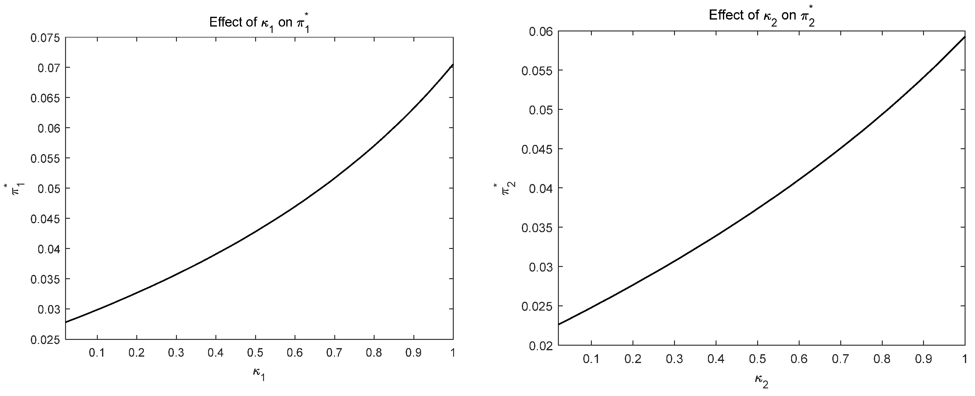
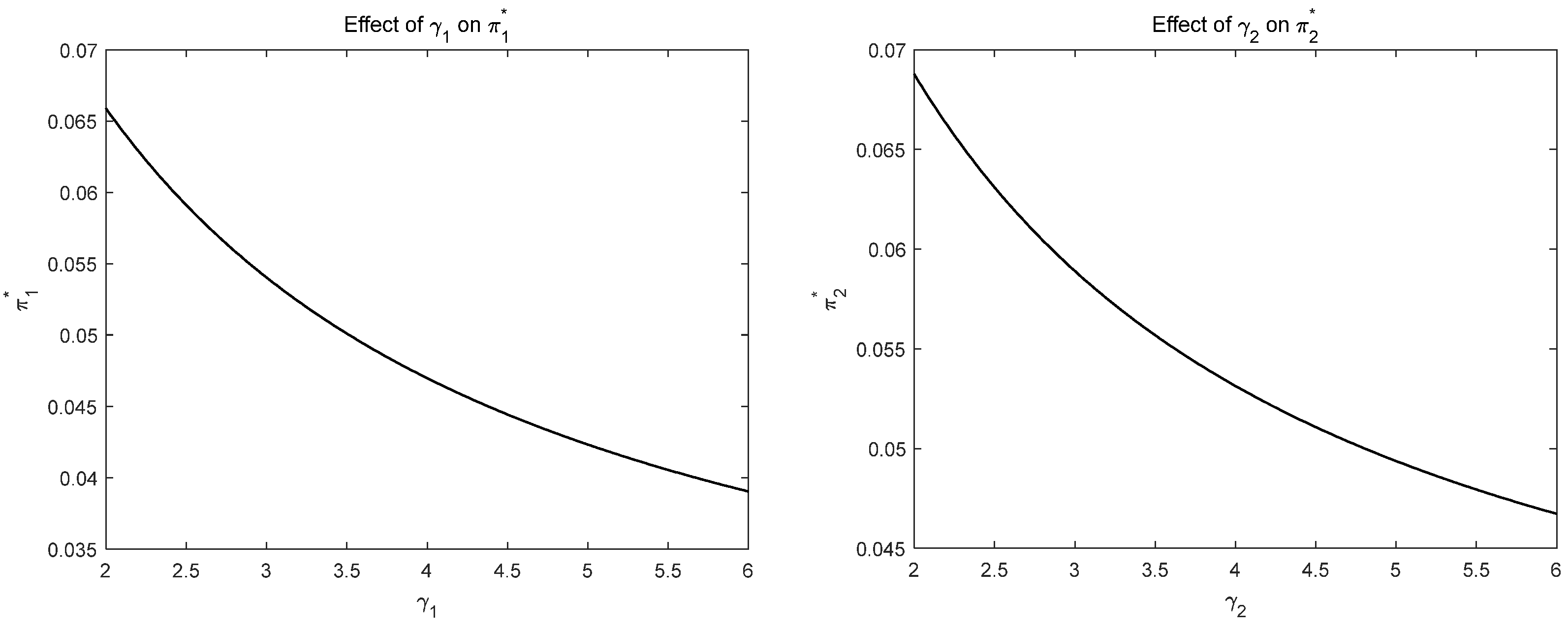
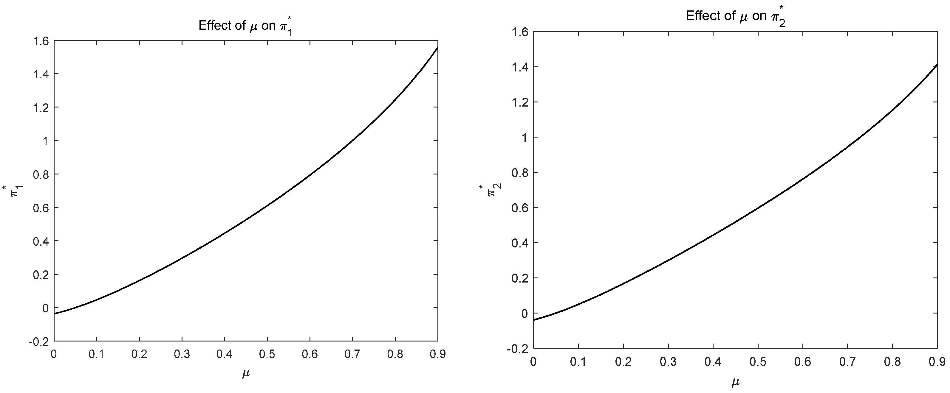
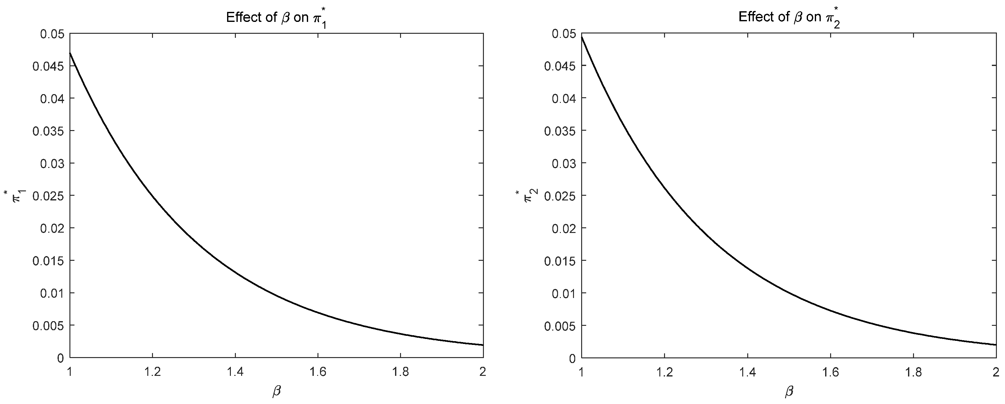
We adopted MATLAB 2022 to carry out numerical calculations, and the results reflecting parameter effects on equilibrium strategies are presented in Figure 1, Figure 2, Figure 3 and Figure 4.

Figure 1 illustrates the impact of the risk aversion coefficient ${\gamma }_k$ on the equilibrium investment strategy ${\pi }_k^{*}(0)$. The graph shows a negative correlation between ${\pi }_k^{*}(0)$ and ${\gamma }_k$, which is consistent with economic intuition. As ${\gamma }_k$ measures investor’s risk preference, a higher ${\gamma }_k$ indicates stronger risk aversion, thereby reducing the proportion of wealth allocated to risky assets.

Figure 2 reveals the impact of the market competition coefficient ${\kappa }_k$ on the equilibrium investment strategy ${\pi }_k^{*}(0)$. The graph indicates that ${\pi }_k^{*}(0)$ rises as ${\kappa }_k$ increases, a monotonic relationship consistent with the findings of Espinosa and Touzi (2015) [3] and Kraft et al. (2020) [19]. The former adopted the CARA utility function to depict investors’ risk attitudes, while the latter applied the CRRA utility function. No matter which utility form is used, a larger ${\kappa }_k$ implies that investors pay more attention to relative wealth. In such cases, to obtain competitive advantages, investors will adopt more aggressive strategies and raise the share of risky assets in their portfolios.

Figure 3 depicts the impact of the expected return μ of the risky asset on the equilibrium investment strategy ${\pi }_k^{*}(0)$. There exists a significant positive correlation: ${\pi }_k^{*}(0)$ grows along with the rise in expected return μ. Intuitively, a higher expected return brings higher potential profits from risky assets, so rational investors will increase their holding of risky assets. This outcome aligns with the basic assumption of rational investors in economics and finance.

Figure 4 illustrates the impact of the parameter $\beta$ on the equilibrium investment strategy ${\pi }_k^{*}(0)$. The figure shows a negative correlation between the two variables. When $\beta$ increases, the price volatility and investment risk of the risky asset will increase. For risk-averse investors, they will accordingly cut down the proportion invested in risky assets, which conforms to the general investment logic of rational market participants.

6. Conclusions

Financial markets are complex and dynamic. To better characterize the volatility features of risky asset prices, this study adopted the CEV model to describe the price dynamics of risky assets, constructing a financial market consisting of one risk-free bond and one risky stock modeled under the CEV framework. Considering the stochastic game interactions between market participants, we establish a two-player non-zero-sum stochastic differential investment game, where investors’ relative performance is defined as the weighted average of terminal wealth ratios. With the dynamic programming principle, we derive the sufficient conditions for the existence of Nash equilibrium and obtain the explicit analytical solutions to equilibrium strategies under the CRRA utility functions. Numerical simulations were carried out to discuss how model parameter affect equilibrium strategies. The simulation results reveal that the expected return of the risky asset, the constant elasticity of variance factor, the risk aversion coefficient, and the market competition parameter all exert significant influence on the equilibrium investment strategies. Specifically, investors tend to increase their allocation to risky assets when the expected return of the risky asset is higher, the constant elasticity of variance factor is smaller, the risk aversion coefficient is lower, or the market competition parameter is larger—and vice versa. To some extent, this indicates that intensified competition in financial markets leads to heightened rivalry among investors, prompting each to increase investments in risky assets and thereby contribute to investment exuberance in financial markets.